Aalborg University

Esbjerg Institute of Technology

Master of Science Thesis

E�cient Supervised Reinforcement

Learning in Backgammon

by

Boris Søborg Jensen

Supervisor: associate professor Daniel Ortiz

Esbjerg, June, 2009

Title

E�cient Supervised ReinforcementLearning in Backgammon

Project period

P10February 2, 2009 - June 10, 2009

Projectgroup

F10s-1

Group members

Boris S. Jensen

Supervisor

Daniel Ortiz-Arroyo

Total number of pages: 60

Abstract

Reinforcement learning is a powerful model

of learning, but has the practical problems

of requiring a large amount of experience,

and bad initial performance of the learner.

This master degree thesis presents a possi-

ble solution to the second of these problems

in the domain of backgammon, where a su-

pervisor is employed to ensure adequate ini-

tial performance, while retaining the ability

of the learning agent to discover new strate-

gies, enabling it to surpass the supervisor.

There is no standard measure for this kind of

improvement, so an ad-hoc measure is pro-

posed, which is used to guide the experimen-

tation. Using this measure shows that su-

pervised reinforcement learning can be used

to solve the problems posed by ordinary re-

inforcement learning in the backgammon do-

main.

Preface

This master degree thesis is written by group F10s-1-F08, at Aalborg University Esbjerg. Theproject theme is Supervised Reinforcement Learning. Part of the code used in this project,namely the neural network implementation has been provided by the NeuronDotNet project[Neu08]. The Pubeval implementation has been adapted from [Tes08].

Reference to other parts of the report will be marked as follows:

• References will be marked like this: Figure 2.1.

• Citations will be marked like this: [Tes95].

The folders on accompanying cd-rom contains the following:

• Articles. Articles cited in the report.

• Thesis. This thesis itself in pdf-format and LATEXformat.

• Source. Source code for the supervised reinforcement learning backgammon controller.

• Results. Excel �les containing the results of the tests described in the report.

The author would like to thank associate professor Daniel Ortiz for great patience and opti-mism.

v

Contents

Contents vi

1 Introduction 1

2 The Backgammon Domain 3

2.1 Introduction . . . . . . . . . . . . . . . . . . . . . . . . . . . . . . . . . . . . 32.2 Backgammon . . . . . . . . . . . . . . . . . . . . . . . . . . . . . . . . . . . 3

2.2.1 Moving . . . . . . . . . . . . . . . . . . . . . . . . . . . . . . . . . . . 42.2.2 Bearing Off . . . . . . . . . . . . . . . . . . . . . . . . . . . . . . . . 42.2.3 Winning . . . . . . . . . . . . . . . . . . . . . . . . . . . . . . . . . . 4

2.3 Complexity . . . . . . . . . . . . . . . . . . . . . . . . . . . . . . . . . . . . . 52.4 A Framework for Backgammon Agents . . . . . . . . . . . . . . . . . . . . 52.5 Conclusion . . . . . . . . . . . . . . . . . . . . . . . . . . . . . . . . . . . . . 6

3 Reinforcement Learning 7

3.1 Introduction . . . . . . . . . . . . . . . . . . . . . . . . . . . . . . . . . . . . 73.2 The reinforcement learning problem . . . . . . . . . . . . . . . . . . . . . . 7

3.2.1 The Return . . . . . . . . . . . . . . . . . . . . . . . . . . . . . . . . . 83.2.2 Markov Decision Processes . . . . . . . . . . . . . . . . . . . . . . . 93.2.3 Value Functions . . . . . . . . . . . . . . . . . . . . . . . . . . . . . . 93.2.4 Generalized policy Iteration . . . . . . . . . . . . . . . . . . . . . . . 103.2.5 Action Selection . . . . . . . . . . . . . . . . . . . . . . . . . . . . . . 11

3.3 Temporal Difference Learning . . . . . . . . . . . . . . . . . . . . . . . . . . 113.3.1 On-policy and Off-policy Algorithms . . . . . . . . . . . . . . . . . 123.3.2 The TD(λ) Algorithm . . . . . . . . . . . . . . . . . . . . . . . . . . 14

3.4 Function Approximation . . . . . . . . . . . . . . . . . . . . . . . . . . . . . 163.4.1 Gradient Descent Methods . . . . . . . . . . . . . . . . . . . . . . . 163.4.2 Tile Coding . . . . . . . . . . . . . . . . . . . . . . . . . . . . . . . . 203.4.3 Kanerva Coding . . . . . . . . . . . . . . . . . . . . . . . . . . . . . 22

3.5 Conclusion . . . . . . . . . . . . . . . . . . . . . . . . . . . . . . . . . . . . . 22

4 Related Work 23

4.1 Introduction . . . . . . . . . . . . . . . . . . . . . . . . . . . . . . . . . . . . 234.2 Two Kinds of Training Information . . . . . . . . . . . . . . . . . . . . . . . 234.3 The RATLE Framework . . . . . . . . . . . . . . . . . . . . . . . . . . . . . 244.4 Supervised Actor-Critic Reinforcement Learning . . . . . . . . . . . . . . . 254.5 Testing . . . . . . . . . . . . . . . . . . . . . . . . . . . . . . . . . . . . . . . 264.6 Conclusion . . . . . . . . . . . . . . . . . . . . . . . . . . . . . . . . . . . . . 27

vi

5 Test De�nition 29

5.1 Introduction . . . . . . . . . . . . . . . . . . . . . . . . . . . . . . . . . . . . 295.2 TD-Gammon . . . . . . . . . . . . . . . . . . . . . . . . . . . . . . . . . . . . 295.3 The Benchmark Opponent . . . . . . . . . . . . . . . . . . . . . . . . . . . . 305.4 Measuring Performance . . . . . . . . . . . . . . . . . . . . . . . . . . . . . 315.5 Conclusion . . . . . . . . . . . . . . . . . . . . . . . . . . . . . . . . . . . . . 32

6 Adapting the Supervised Actor-Critic Learning Model 33

6.1 Introduction . . . . . . . . . . . . . . . . . . . . . . . . . . . . . . . . . . . . 336.2 The Supervised Actor-Critic Reinforcement Learning Model . . . . . . . . 346.3 Adapting the Model to Backgammon . . . . . . . . . . . . . . . . . . . . . . 356.4 K-values . . . . . . . . . . . . . . . . . . . . . . . . . . . . . . . . . . . . . . 36

6.4.1 Kanerva Coding . . . . . . . . . . . . . . . . . . . . . . . . . . . . . 366.4.2 Neural Networks . . . . . . . . . . . . . . . . . . . . . . . . . . . . . 386.4.3 State Independent Interpolation . . . . . . . . . . . . . . . . . . . . 38

6.5 Conclusion . . . . . . . . . . . . . . . . . . . . . . . . . . . . . . . . . . . . . 39

7 Test 41

7.1 Introduction . . . . . . . . . . . . . . . . . . . . . . . . . . . . . . . . . . . . 417.2 Test Results . . . . . . . . . . . . . . . . . . . . . . . . . . . . . . . . . . . . 417.3 Conclusion . . . . . . . . . . . . . . . . . . . . . . . . . . . . . . . . . . . . . 43

8 Conclusion 45

Appendices 47

A N-ply Search 49

Bibliography 51

Chapter 1

Introduction

Machine learning is often based on the same principles as human learning. Imagine for in-stance a boy, trying to throw a ball through a ring. One way to for the boy to learn this, isto just throw the ball and observe what happens. At �rst the results will seem random, butlittle by little, the aim and throw will get better, as the boy learns by experience, what doesand does not work. This is the basic principle behind the �eld of machine learning known asreinforcement learning: Learning comes from interacting with the environment.

This simple principle gives rise to the reinforcement learning model, in which an agent inter-acts with the environment by performing actions dependent on the state of the environment.The environment responds by changing its state and by rewarding the agent with a scalarreward signal. The learning occurs, as the agent tries to maximize the cumulative reward overtime. The simplicity of this model makes it possible to apply reinforcement learning to a widevariety of situations. Examples of domains, where reinforcement learning has been appliedsuccesfully, include dynamic channel allocation for cellphones [SB97], elevator dispatching[CB96] and backgammon [Tes95]. In the case of the backgammon domain, Gerald Tesaurocreated the TDGammon player, which is based on a reinforcement learning technique calledtemporal-di�erence learning. TDGammon eventually reached a playing strength that rivalsor perhaps even surpasses that of human world class backgammon master players, and someof its tactics have even been adopted by these players. One of the surprising lessons learnedfrom TDGammon was, that it could achieve this high level of performance, even though ithad started out knowing nothing about the game, and had only learned through self-play, i.e.playing both sides of the board.

As powerful as the reinforcement learning principle may be, there are still some drawbacks.They are related to the fact that, starting from scratch, it can take a long time to reach anacceptable level of performance. This can be annoying in learning from simulated experience,where the amount of simulations required can prohibit extensive testing of variations - the ver-sion of TDGammon, that reached master level, played 6.000,000 games against itself[Tes02]- but the real problems arise when the actions are performed in a real environment. Here, itmay be very di�cult to obtain the required amount of experience, and the consequences ofnot performing at an adequate level may be severe, depending on the domain.

What can be done to avoid these drawbacks? An answer may be found by considering, thatthe reinforcement learning principle is not the only mode of learning. Humans can also learnfrom teachers, either by mimicking them, or by receiving advice or evaluations from them. In

1

the example of the ball-throwing boy, imagine the situation when a parent or teacher is nearbyto demonstrate the throw, or give praise, when the boy has the correct posture. In such asituation, the boy might learn faster, and the �rst shots will likely not be as bad, since theteacher will guide them. With such a setup, it is important, that the teacher at some time,when the boy has become pro�cient, becomes less involved, leaving the boy to discover byexperience more advanced techniques and skills, that may even surpass those of his teacher.Such a mode of learning could be called supervised reinforcement learning.

Fortunately, in many cases it is possible to formulate simple heuristics that may act as ateacher to a computer program trying to learn by reinforcement. The purpose of this reportis to explore how supervised reinforcement learning can be applied to improve the results ofTDGammon. Chapter 2 describes the game of backgammon, while chapter 3 describes howreinforcement learning can be treated mathematically. The classic reinforcement theoreticalcorpus is concerned with state spaces, that can comfortably be represented in a table, butreal world problems, including that of learning to play backgammon, often operate in statespaces that are much too large to practically �t in any table, so a later section of the chapteradresses the practical problem of how to learn anything in a state space as vast as that ofbackgammon. Chapter 4 describes the other work done, and the challenges faced in the �eldof supervised reinforcement, as well as how the task of improving TDGammon compares toother tasks that supervised reinforcement learning has been used to solve. This comparisonshows that there is a need for a custom testbed to measure the improvements achieved,so chapter 5 provides one such measure. Since the measure is custom made, it cannot beused for comparing with previous results in related work, but it can be used as a guide forexperiments within this report. Chapter 6 uses the previous knowledge to produce threemodels of supervised reinforcement learning for the backgammon domain. These models onlydi�er in the method by which the teacher gradually withdraws, as the learning agent becomesmore knowledgeable. The models are tested in chapter 7, and �nally chapter 8 sums up thefeasibility of using supervised reinforcement learning to improve the results of TDGammon.

Chapter 2

The Backgammon Domain

2.1 Introduction

This chapter introduces the rules of the game of backgammon. This is done in section 2.2and provides the basic understanding required of the next two sections. Section 2.3 discussesthe complexity involved in playing well, and section 2.4 shows how the game mechanics canbe used to specify how the backgammon agents should interact. In the following, the termsplayer and agent will be used interchangeably.

2.2 Backgammon

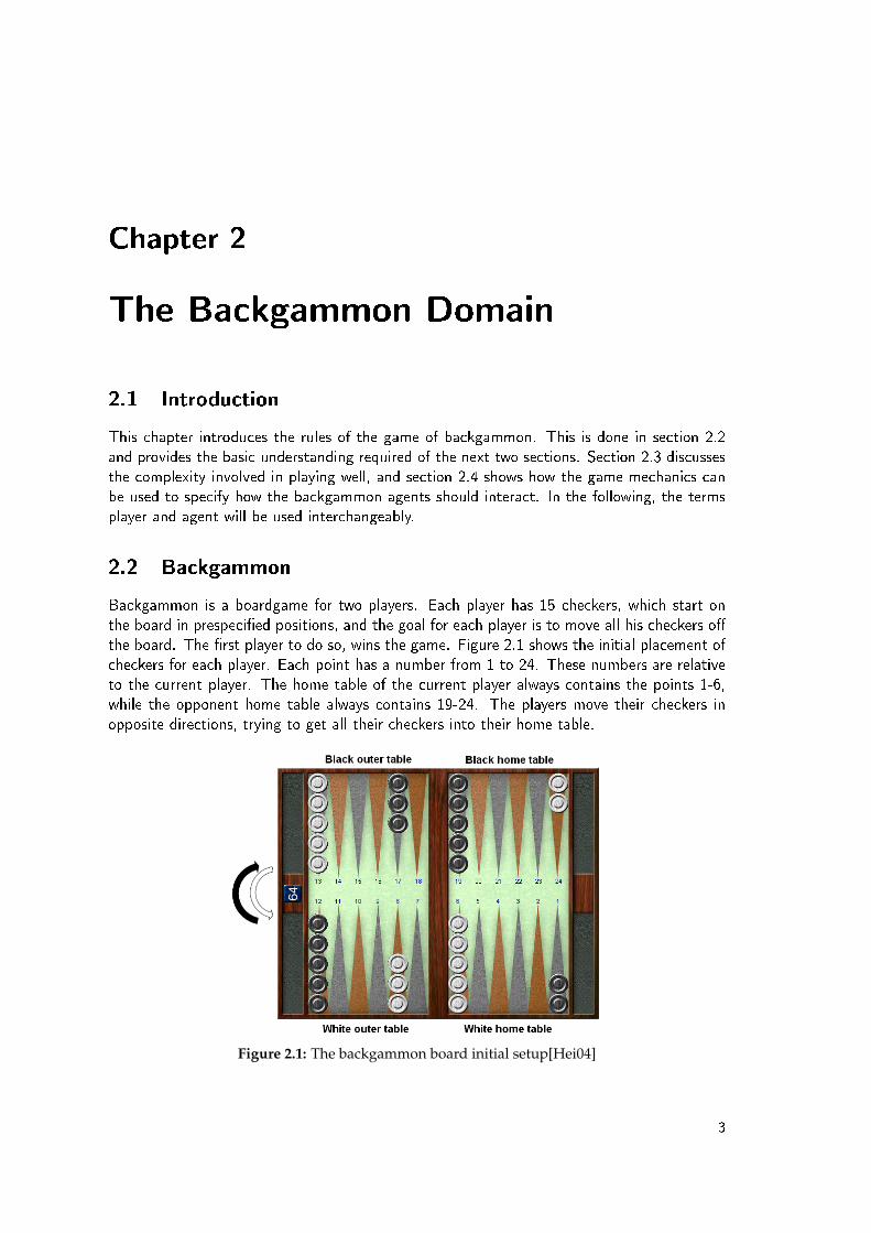
Backgammon is a boardgame for two players. Each player has 15 checkers, which start onthe board in prespeci�ed positions, and the goal for each player is to move all his checkers o�the board. The �rst player to do so, wins the game. Figure 2.1 shows the initial placement ofcheckers for each player. Each point has a number from 1 to 24. These numbers are relativeto the current player. The home table of the current player always contains the points 1-6,while the opponent home table always contains 19-24. The players move their checkers inopposite directions, trying to get all their checkers into their home table.

Figure 2.1: The backgammon board initial setup[Hei04]

3

2.2.1 Moving

The players take turns to move their checkers. Each turn, a player throws 2 dice. Unlessa double is thrown, two moves are allowed, one for each die. If a double is thrown, then 4moves are allowed, each move using the number of pips on one of the dice, e.g. if a double 5is thrown, then the player has 4 moves of 5 points each. These moves can be combined freely,i.e. the moves can be divided on di�erent checkers, or a single checker can use more than oneof the available moves. Multiple moves are carried out consecutively, e.g. using 3 moves of 5doesn't count as making a single move of 15. A player is not allowed to pass on his moves,as many moves as possible must be made each turn. If a point is occupied by two or morecheckers, then they are safe, and no move by the opposing player may land at that point. If apoint is occupied by a single checker, that is called a blot, and the checker is vulnerable to ahit by the opposing player. Checkers are hit if the opposing player moves a checker onto theblot checker point. Checkers, that are hit, are moved to the bar, that divides the outer tablefrom the home table, and from here they must enter the home table of the opposing player.Entering the opposing players home table counts as a normal move, e.g. using a move of 1lands the checker on the 24 point. While a player still has checkers on the bar, he may notmove any other checkers.

2.2.2 Bearing O�

Once a player has all his checkers in his own home table, he may start to remove them fromthe game. This is known as bearing o�. Using a move of 1 will bear o� a checker from the 1point, using a move of 2 will remove a checker from the 2 point and so on. A player doesn'thave to bear o�, he may also spend available moves moving checkers inside his home table.If the player has an available move, that is higher than the highest point, at which the playerstill has checkers, then he may use that move to bear o� a checker from the that point. If atany time the opposing player captures a checker, then the player cannot continue to bear o�,before all his checkers are again in his home table.

2.2.3 Winning

The �rst player to bear o� all his checkers wins the game and the current stake. The normalstake to be won is 1 point. This stake can be modi�ed in two ways: By winning veryimpressively or by using a special die called the doubling cube. If the opposing player has notyet borne o� any of his checkers, then the player has won a "`gammon"', which doubles thestake. If the opposing player still has checkers on the bar, or in the players home table, thenthe player has won a "`backgammon"', which triples the stake instead. The doubling cube isa die, whose side shows the numbers 2, 4, 8, 16, 32 and 64, representing the current value ofthe stake. When it is his turn, a player may o�er to double the stake, before he throws thedice. If this o�er is accepted by the opposing player, then current stake is doubled, and thedoubling cube is used to indicate this. If the opposing player rejects the o�er, then the playerwins the current stake before the doubling. Initially, any player can make the doubling o�er,but once the stake has been doubled, only the opposing player is allowed the next doublingo�er.

2.3 Complexity

Strategically, backgammon can be divided into two distinct phases: The contact phase and therace phase. The game starts in the contact phase, and the race phase then occurs, when thelast checkers of each player have passed each other, removing any possibility for the players tohit the opponent's checkers, or block their path. The strategy of the race phase thus reducesto setting up the checkers in the home table, such that all moves can be fully utilized whenbearing o�. The contact phase on the other hand requires the weighing of several subgoals.For instance, it is often desirable to hit an opponents checker, but if the player has many singlecheckers in his home table, it may not be such a good idea, since the opponent in his next turnmay be able to hit those checkers in return. This could be a bad trade, since the player usuallyhas spent a number of moves on checkers in his home table. Another consideration is build-ing blockades, or primes, which are consecutive positions, where the player has two or morecheckers. Long primes impedes the opponents checkers, since the prime must be traversed ina single move. It is therefore important to have a �exible position, that allows using the futuredice rolls to build a prime. Obtaining this �exible position, however, can mean exposing singlecheckers to being hit by the opponent, leading to a con�ict between the goals of buildingprimes and avoiding blots. To obtain good performance, such concerns must be addressedappropriately for each of the board states, that are encountered during a game. The numberof possible states in backgammon is estimated to be in the order of 1020[Tes95]. A lot of thesestates have an extremely small likelihood of occuring during a normal game, so in reality thenumber of states, for which an agent needs to have good judgement is much smaller, but thenumber of states, that can reasonably be expected to occur in a normal game is still very high.

Another source of complexity is the branching factor. One way to evaluate the consequencesof a given move is to imagine the possible scenarios that might occur after the move. This iscalled searching the game tree. The nodes of a game tree are board states, and the childrenof a node are all the states that might occur as the result of a player taking a turn fromthat state. The feasibility of game tree search is bounded by the branching factor, whichis the average number of children of a node in the tree. The average number of moves inbackgammon, given a certain dice combination, is around 20 [Tes95], and since the numberof e�ectively di�erent dice combinations is 21, backgammon has a branching factor of around400, which in practice limits the depth, to which the game tree can be searched, to 2 or 3.

2.4 A Framework for Backgammon Agents

Backgammon can be seen as a system with partial knowledge of the dynamics: The actionof making a move leads with certainty to a new state, called the afterstate, at which pointthe opponent takes his turn by rolling the dice, and making his move. The opponents turncan be seen as a probabilistic system response. The important thing to realize here is, thatthis system response is dependent only on the afterstate. Stated another way, the expectedsystem response is the same for two board state/dice roll combinations, that lead to the sameafterstate. This means that the utility of an afterstate will be the same as that of all thestate/dice combinations that lead to such an afterstate. Therefore it makes sense to onlyevaluate the afterstates, since that reduces the size of the total state space by a factor of 21.

A way to implement this would be to have a central backgammon playing framework, thatrolls the dice for each player, and generates the possible board states, that can be reached

from the current board with the new dice. The job of an agent is then only to evaluate theboard states that are presented to it. This is the way, that TDGammon was implemented[SB98]. Using these evaluations, the framework can then decide which move to make forthe player. The obvious choice would be to choose the move with the highest evaluation,but in some situations it may be advantageous to make another move. This is due to thedilemma between exploitation and exploration. Exploitation refers to choosing the move,that the player thinks is best, while exploration tries to expand the knowledge of the playerby choosing a move, that may lead to some states which the player is not familiar with.Exploitation will maximize the expected reward in the short run, while a certain amount ofexploration will be bene�cial in the long run, since the player may discover that some moveswere better, than previously expected. However, too much exploitation will lead to the playerconsistently choosing sub-optimal moves, leading to decreased long-term performance.

2.5 Conclusion

Backgammon is a game with simple rules, but with some game mechanics, that make it avery complex game. This complexity arises from the task of managing con�icting goals suchas hitting an opponent and/or building a �exible position versus avoiding blots. The highbranching factor also contributes to the complexity by making it di�cult to consider all thepossible scenarios more than two or three steps into the future. Another factor is the di-mensionality of the problem. A backgammon board can be fully characterized by an array of24 integers, encoding the number of checker on each board location, plus information aboutcheckers on the bar. 24 is already a considerable number of dimensions, but this relativelycompact encoding is highly non-linear. For instance, there is a very large di�erence in thetactical value between positions with a single checker, and positions with two checkers, whilethe di�erence is much less between four checkers and �ve. As will be shown in chapter 5,TDGammon overcomes this problem by speci�cally encoding, whether there is a blot, but thisonly serves to increase the dimensionality of the problem.

The fact, that backgammon is a game with partial knowledge of the dynamics makes it possibleto reduce some of this complexity. Speci�cally, it is not necessary for the agent to have anyknowledge of dice rolls; by presenting only afterstates to the agents, move decisions can bemade without any loss of performance. Another decision, that can be made easier throughknowledge of the game mechanics, is that of exploration versus exploitation. Backgammonalready provides a sort of exploration mechanism through the dice rolls. The dice ensure, thatit is very unlikely for the same two players to experience the exact same sequence of boardstates twice, even though their policies have not changed. Therefore, although the optimaldegree of exploration is di�cult to determine, a practical rule is for the framework to disregardany further exploration, and just choose the exploiting move, i.e. the move that has receivedthe highest score from the agent.

Chapter 3

Reinforcement Learning

3.1 Introduction

Many machine learning techniques require examples of correct behaviour, that are to beimitated and extrapolated. Reinforcement learning[SB98] is a set of learning methods, thatdo not require such examples. Instead, the idea behind reinforcement learning is to learnby interaction with an environment, using feedback to adjust the choice of actions. Section3.2 will explain the basic reinforcement learning problem. Section 3.3 describes temporaldi�erence learning, which is a very succesful reinforcement learning method, and �nally section3.4 describes how function approximators such as arti�cial neural networks can be used inreinforcement learning to cope with large state spaces.

3.2 The reinforcement learning problem

In reinforcement learning, the focus is on learning through interaction. The learner anddecisionmaker is called the agent, and it interacts with the environment, which compriseseverything outside the agent. The interaction is cyclic: The environment is in a certain state,leading the agent to take an action, which changes the state of the environment, leading tonew actions and so on. The environment also responds to the actions of an agent with ascalar reward signal, according to the action taken. A full speci�cation of the environmentwith reward and state transition functions is called a reinforcement learning task.

A natural formulation of the reward function in the domain of backgammon is to award zeropoints for moves, that do not either win or lose, 1, 2 or 3 points for moves, that lead directlyto winning the game, and -1, -2 or -3 points for moves after which the opponent directly winsthe game. Once an opponent has been speci�ed, the state transitition function is also easilyde�ned: The opponent acts as the environment, making changes to the board according tohis own policy.

The agent and the environment can interact at each of a sequence of discrete time stepst = 0, 1, 2, .... At each time step t, the agent receives some representation of the environmentstate, st ∈ S, where S is the set of states of the environment. In response to the received staterepresentation, the agent takes an action at ∈ A, where A is the set of actions available to theagent. At time t + 1 the agent then receives a scalar reward rt+1, and �nds itself in a new statest+1. rt+1 and st+1 are both partially dependent on st and at. This interaction is shown on�gure 3.1. At each time step t, the agent implements a function πt(a, s) = Pr(at = a|st = s).

7

This function is called the agents policy.

Figure 3.1: The interaction between an agent and its environment[SB98]

3.2.1 The Return

Reinforcement learning is concerned with changing the policy, such that the expected value ofsome aggregation of the reward sequence, starting at time t, is maximized. This aggregationis called the return, and is denoted Rt. There are a number of ways to de�ne the return. Anatural way could be to de�ne the return as

Rt = rt+1 + rt+2 + · · ·+ rT =T

∑k=1

rt+k, (3.1)

where T is a �nal time step. This makes sense in tasks that have a natural notion of a �naltime step, such as games, where winning or loosing the game causes a transition to a terminalstate sT. Such tasks are called episodic tasks. For tasks, that have no terminal state, suchas an ongoing control process, simply adding the received reward could cause the return togrow unbounded. Therefore, the return for non-episodic tasks are often de�ned as

Rt = rt+1 + γrt+2 + γ2rt+3 + · · · =∞

∑k=0

γkrt+k+1. (3.2)

This is called the discounted return, and the parameter γ ∈ [0, 1] is called the discountingrate. Adjusting the γ parameter corresponds to adjusting how the agent weighs the di�erentrewards in the sequence. If γ is 0, then the agent considers only the reward from the nextaction. As γ increases, more weight is put on rewards farther in the future. When γ is 1,the agent considers all rewards equally, but this requires, that the sum of rewards is bounded.The return for the episodic task can also be represented as a special case of the return for thenon-episodic task, using a γ of 1, and with the convention, that terminal states transition tothemselves, yielding rewards of 0, as exempli�ed in �gure 3.2.

Figure 3.2: Episodic task with terminal state transitions[SB98]

The backgammon task is a good example of an episodic task. The game has a clear ending,after which point no more rewards can be earned, and the reward is only non-zero just when

the game ends. Therefore the total reward is always bounded, and there is no need for adiscount. In fact, using a discount would not be good, since the �rst states encounteredwould receive more reward from winning a short game, than a long game, although the onlygoal is to win the game, no matter the lenght.

3.2.2 Markov Decision Processes

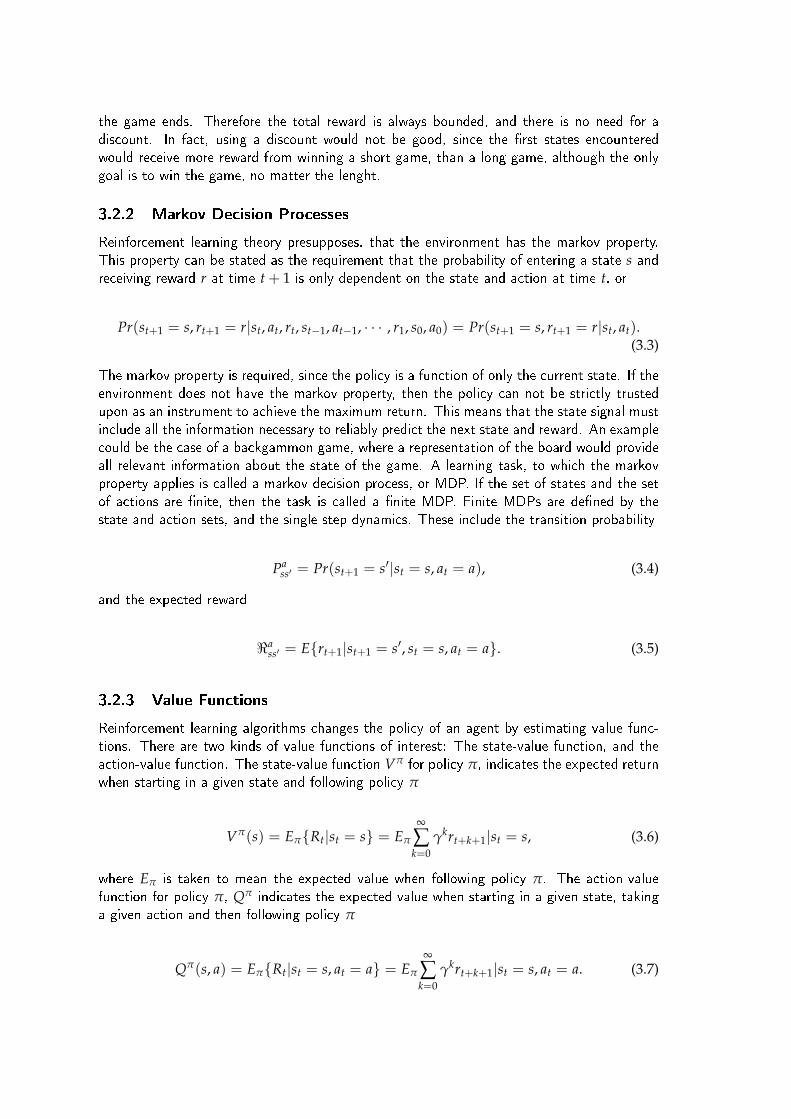
Reinforcement learning theory presupposes, that the environment has the markov property.This property can be stated as the requirement that the probability of entering a state s andreceiving reward r at time t + 1 is only dependent on the state and action at time t, or

Pr(st+1 = s, rt+1 = r|st, at, rt, st−1, at−1, · · · , r1, s0, a0) = Pr(st+1 = s, rt+1 = r|st, at).(3.3)

The markov property is required, since the policy is a function of only the current state. If theenvironment does not have the markov property, then the policy can not be strictly trustedupon as an instrument to achieve the maximum return. This means that the state signal mustinclude all the information necessary to reliably predict the next state and reward. An examplecould be the case of a backgammon game, where a representation of the board would provideall relevant information about the state of the game. A learning task, to which the markovproperty applies is called a markov decision process, or MDP. If the set of states and the setof actions are �nite, then the task is called a �nite MDP. Finite MDPs are de�ned by thestate and action sets, and the single step dynamics. These include the transition probability

Pass′ = Pr(st+1 = s′|st = s, at = a), (3.4)

and the expected reward

<ass′ = E{rt+1|st+1 = s′, st = s, at = a}. (3.5)

3.2.3 Value Functions

Reinforcement learning algorithms changes the policy of an agent by estimating value func-tions. There are two kinds of value functions of interest: The state-value function, and theaction-value function. The state-value function Vπ for policy π, indicates the expected returnwhen starting in a given state and following policy π

Vπ(s) = Eπ{Rt|st = s} = Eπ

∞

∑k=0

γkrt+k+1|st = s, (3.6)

where Eπ is taken to mean the expected value when following policy π. The action-valuefunction for policy π, Qπ indicates the expected value when starting in a given state, takinga given action and then following policy π

Qπ(s, a) = Eπ{Rt|st = s, at = a} = Eπ

∞

∑k=0

γkrt+k+1|st = s, at = a. (3.7)

Such value functions can be approximated through experience. As an example, in an episodictask, the value of a state s for a given policy π can be approximated as the average returngained from starting a number of times in s and following policy π. This form of reinforcementlearning is called a Monte Carlo method. For most tasks, it makes more sense to estimatethe action-value function, since that makes it easier to �nd the best action to take in a givenstate. However, for the backgammon domain, it is possible to take advantage of the after-states, discussed in chapter 2, to �nd the best move using only a state-value function. Thismove can be de�ned as arg maxs∈SL Vπ(s), where SL is the set of all legal moves.

Value functions impose a partial ordering on the set of possible policies. A policy π is betterthan another policy π′, if Vπ(s) > Vπ′(s) for all s ∈ S. There is always at least one policythat is better than or equal to all other policies. This can be seen by considering that twopolicies π′ and π′′, for which there is no ordering relation, can be combined to create a newpolicy π′′′, that is better than both, by letting π(s, a)′′′ = arg maxπ∈{π′,π′′} Vπ, ∀s. A policy,that is better than or equal to all other policies is called an optimal policy, and is denoted π∗.Such an optimal policy in turn gives rise to an optimal state-value function V∗

V∗(s) = maxπ

Vπ(s) (3.8)

and an optimal action-value function Q∗

Q∗(s, a) = maxπ

Qπ(s, a) (3.9)

3.2.4 Generalized policy Iteration

As previously stated, the value function for a given policy can be estimated through expe-rience. At the same time, each value function determines an optimal policy with regard tothat value function. This suggests, that reinforcement learning can be seen as two concurrentprocesses. In the �rst process, the agent has a value function V, and a policy π, that isoptimal with regard to V. Through experience, V is updated towards the true value functionfor policy π, Vπ. Updating the value function may lead to the policy π no longer being theoptimal policy with regard to V. Thus, the second process updates π towards the optimalpolicy for the updated V. If the �rst process causes π to be suboptimal with regard to V,then the second process will strictly improve π, bringing it closer to an optimal policy π∗.If the second process causes π to improve, then the �rst process will drive V towards V∗.Therefore, the only stable point for these processes are, when the value function is the optimalvalue function, and the policy is the optimal policy. The situation is shown in �gure 3.3.

This concept is called the generalized policy iteration, and is used in almost every reinforce-ment learning method. The methods can di�er in how long they allow each process to run,before changing to the other process. In the reinforcement learning method known as dy-namic programming, which requires knowledge of Pa

ss′ and of <ass′ , V is updated fully towards

V∗ before the policy is updated. In other methods, the two processes may be much moreintermingled, with each update of V being followed by an update of π.

Figure 3.3: Generalized policy iteration: policy and value function interact, until they are consis-tent at the optimal value function and policy[SB98]

3.2.5 Action Selection

It is important to note, that generalized policy iteration can only converge to the optimalpolicy and value functions, if every state/action pair is visited repeatedly, until the functionsreach optimality. This raises precisely the question of exploration versus exploitation, alreadydiscussed in chapter 2. A natural choice in the backgammon domain would be to disregardany exploration other than what is already imposed by the random dice rolls, but there areother options, that make even more explorative moves. These are known as soft-max policyfunctions. Such a function gives higher probability to the best actions, but gives a non-zeroprobability to even the worst action. A common soft-max policy, that uses an action-valuefunction is the Boltzmann distribution:

πBoltzmann(s, a) =eQ(s,a)/τ

∑a′∈A eQ(s,a)/τ(3.10)

Here, τ is a positive constant called the temperature, which in�uences the amount of explo-ration. As τ → ∞, the actions become almost equiprobable, causing greater exploration. Asτ → 0, the policy goes toward the greedy policy, causing greater exploitation. It can be di�-cult to judge the amount of exploitation at a given temperature. Therefore, another soft-maxpolicy commonly used is the simpler ε-greedy policy, which almost always chooses the greedyaction, but with a small percentage ε chooses evenly among all the available actions. Thismakes it simpler to control the amount of exploration being performed, but has the downside,that exploration is just as likely to choose the worst action as the second-best action, which,depending on the environment, can be undesirable.

3.3 Temporal Di�erence Learning

This section describes temporal di�erence learning methods, which is a subset of reinforcementlearning methods. Temporal di�erence methods also use the generalized policy iteration, andrely on the fact that the value function Vπ of a policy π can be expressed recursively. Usingthe de�nition of the state-value function given in equation 3.6 yields:

Vπ(s) = Eπ{Rt|st = s} (3.11)

= Eπ{∞

∑k=0

γkrt+k+1|st = s} (3.12)

= Eπ{rt+1 +∞

∑k=0

γkrt+k+2|st = s} (3.13)

= Eπ{rt+1 + γVπ(st+1)|st = s} (3.14)

Temporal di�erence methods use this recursive relationship to make updates to the valuefunction, according to the following update formula called the TD(0) algorithm

V(st) = V(st) + α(rt+1 + γV(st+1)−V(st)) (3.15)

where α ∈]0, 1] is called the stepsize, or the learning rate. The formula can be intuitivelyunderstood by realizing that V(st) and rt+1 + γV(st+1) are actually both estimates of thevalue function at time t. The only di�erence is, that while V(st) is based on an estimate ofall the future rewards, rt+1 + γV(st+1) includes knowledge of the �rst of these rewards. Ittherefore makes sense to trust the latter estimate more than the �rst, since they are otherwisethe same. This trust is expressed by updating the value function by an amount (positively)proportional to the di�erence (rt+1 + γV(st+1))−V(st), which is called the temporal di�er-ence error. The value of V at s = st is adjusted in the direction of rt+1 + γV(st+1), which istherefore called the target of the update.

Note however, that the target should not be trusted too much. After all, in general the rewardis only a probabilistic function of st, at and st+1, and st+1 itself is a probabilistic functionof st and at, so the reward just received could be very atypical. This is the reason, that thestepsize should not be 1. In fact, updating according to this rule will cause V to convergeto vπ in the mean only if the stepsize is su�ciently small, and with probability 1 only if thestepsize α decreases with time[SB98].

3.3.1 On-policy and O�-policy Algorithms

Using TD(0), it is possible to de�ne a complete reinforcement learning control algorithm,based on temporal di�erence methods and action value functions:

• Initialize Q(s, a) arbitrarily

• Repeat for each episode

– Initialize s

– Choose a from s, using policy derived from Q (e.g. ε-greedy)

– Repeat for each step of episode

∗ take action a, observe reward r and next state s′

∗ Choose action a′ from s′, using policy derived from Q (e.g. ε-greedy)

∗ Q(s, a)← Q(s, a) + α[r + γQ(s′, a′)−Q(s, a)]∗ s← s′, a← a′

This algorithm is called sarsa, because it uses all the elements (st, at, rt+1, st+1, at+1) thatde�ne a transition from one state to the next. Sarsa will converge to the optimal valuefunction on two conditions. First, every state/action pair must be visited recurringly. Thiscan be achieved with a softmax policy such as ε-greedy. The second convergence criterium isthat the policy must converge in the limit to the greedy policy. This can be achieved for the ε-greedy policy by letting ε = 1

t . Sarsa is an on-policy algorithm, because the action suggestedby the policy is used both to transition to another state and to update the action-valuefunction. This is in contrast to an o�-policy algorithm such as the Q-learning algorithm:

• Initialize Q(s, a) arbitrarily

• Repeat for each episode

– Initialize s

– Repeat for each step of episode

∗ Choose a from s, using policy derived from Q (e.g. ε-greedy)

∗ take action a, observe reward r and next state s′

∗ Q(s, a)← Q(s, a) + α[r + γ maxa′ Q(s′, a′)−Q(s, a)]∗ s← s′

Here, the policy is responsible for which state/action pairs are updated, but not for the valuewith which they are updated. The only criterium for convergence of Q towards Q∗ is thereforethat every state/action pair is visited recurringly.

The di�erence between an on-policy and an o�-policy algorithm is best shown by example.The example task is walking on the edge of a cli�, getting to the other end as fast as possible.The task is episodic, stopping when the other end of the cli� has been reached. To encouragegetting to the end as fast as possible, the reward for each step is -1, while the reward forfalling o� the cli� is -100. The state set is a grid as shown in �gure 3.4, and the actions areup, down, right and left. Every action leads deterministically to the next state in the indicateddirection, except for except for any action, that goes over the cli� edge, which leads back tothe start state S. The state set contains a single terminating state, marked with G. Figure3.5 shows the performance of sarsa and Q-learning algorithms over the task, using ε-greedyalgorithms with a �xed ε of 0,1. The sarsa algorithm learns the safe path, yielding higherresults than the Q-learning algorithm, which actually learns the optimal path, but has lowerperformance than sarsa due to the softmax policy. Of course, if ε converged towards 0, thenthe performance of both algorithms would approach the optimum.

Figure 3.4: A cliff walking task[SB98]

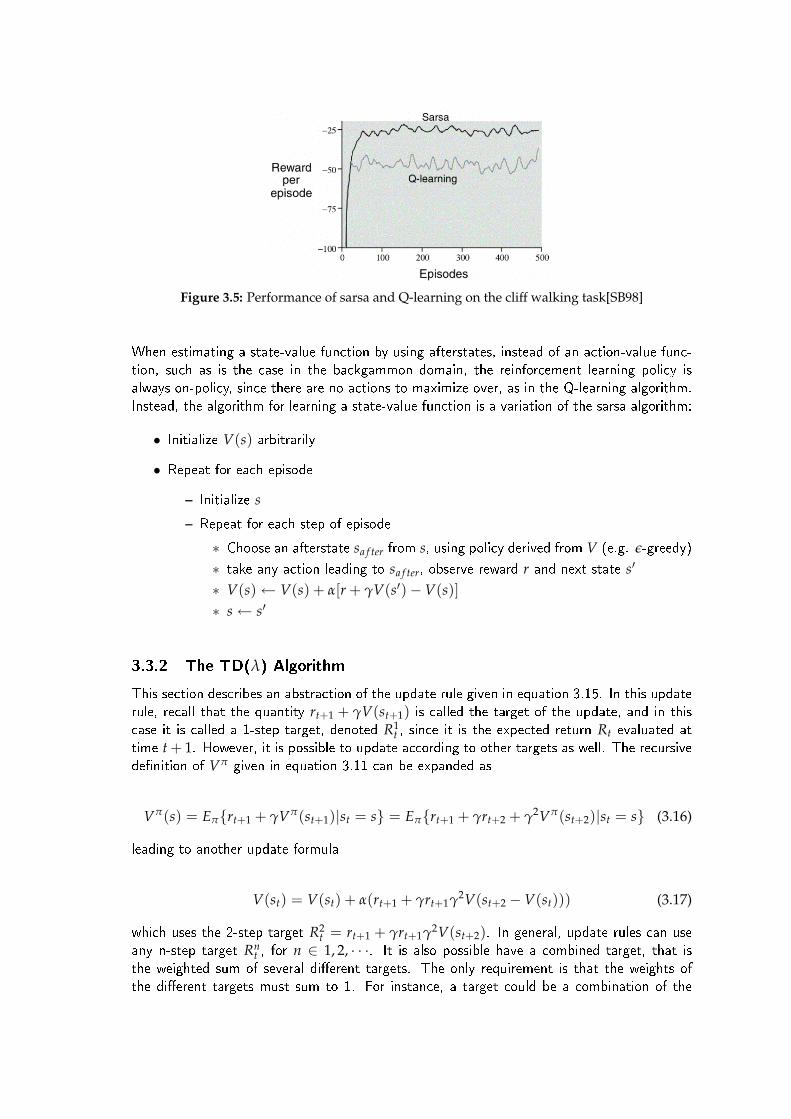
Figure 3.5: Performance of sarsa and Q-learning on the cliff walking task[SB98]

When estimating a state-value function by using afterstates, instead of an action-value func-tion, such as is the case in the backgammon domain, the reinforcement learning policy isalways on-policy, since there are no actions to maximize over, as in the Q-learning algorithm.Instead, the algorithm for learning a state-value function is a variation of the sarsa algorithm:

• Initialize V(s) arbitrarily

• Repeat for each episode

– Initialize s

– Repeat for each step of episode

∗ Choose an afterstate sa f ter from s, using policy derived from V (e.g. ε-greedy)

∗ take any action leading to sa f ter, observe reward r and next state s′

∗ V(s)← V(s) + α[r + γV(s′)−V(s)]∗ s← s′

3.3.2 The TD(λ) Algorithm

This section describes an abstraction of the update rule given in equation 3.15. In this updaterule, recall that the quantity rt+1 + γV(st+1) is called the target of the update, and in thiscase it is called a 1-step target, denoted R1

t , since it is the expected return Rt evaluated attime t + 1. However, it is possible to update according to other targets as well. The recursivede�nition of Vπ given in equation 3.11 can be expanded as

Vπ(s) = Eπ{rt+1 + γVπ(st+1)|st = s} = Eπ{rt+1 + γrt+2 + γ2Vπ(st+2)|st = s} (3.16)

leading to another update formula

V(st) = V(st) + α(rt+1 + γrt+1γ2V(st+2 −V(st))) (3.17)

which uses the 2-step target R2t = rt+1 + γrt+1γ2V(st+2). In general, update rules can use

any n-step target Rnt , for n ∈ 1, 2, · · ·. It is also possible have a combined target, that is

the weighted sum of several di�erent targets. The only requirement is that the weights ofthe di�erent targets must sum to 1. For instance, a target could be a combination of the

1-step and 2-step targets, such that the update rule would be V(st) = V(st) + α(Rcombinedt −

V(st))), where Rcombinedt = 1

2 R1t + 1

2 R2t . This idea of combining targets give rise to the TD(λ)

algorithm, for λ ∈ [0, 1], which updates according to the target Rλt which is a weighted mixture

of in�nitely many targets:

Rλt = (1− λ)

∞

∑n=1

λn−1Rnt (3.18)

The (1− λ) factor is prepended to the in�nite sum to make the weights sum to 1. Updatesmade according to the Rλ

t target take into account a weighted sum of all the di�erent esti-mates of the return received after time t. The function of the λ parameter is to control howthese estimated returns are weighted. The TD(0) method, shown in equation 3.15 only usesthe R1

t target, but for λ > 0 the other return estimates gain more weight, and as λ goes to1, the returns are given almost equal weight.

The purpose of updating according to an in�nite mixture of targets is to learn more e�ciently.In principle, the idea may have some merit. But in practice, it may seem quite ine�cient:The target can only be fully evaluated in the context of an episodic task, only when the taskis �nished, and until then it is necessary to remember all the received rewards. However,equation 3.18 can be transformed to an incremental update rule, using a mechanism knownas eligibility traces. The idea that visiting a state makes it eligible to receive updates from allthe future rewards. The weight of each of these rewards in the Rλ

t target can be calculated, sowhen a reward is received, the value function can be incrementally updated. The importantthing is to remember how much reinforcement a state should receive from each new reward.This weight can also be calculated incrementally, and is called the the eligibility trace of thestate. The full TD(λ) algorithm is as follows:

• Initialize V(s) arbitrarily

• Set e(s) = 0∀s

• Repeat for each episode:

– Initialize s

– Repeat for each step of episode:

∗ Choose an afterstate sa f ter from s, using policy derived from V (e.g. ε-greedy)

∗ take any action leading to sa f ter, observe reward r and next state s′

∗ δ← r + γV(s′)−V(s)∗ e(s) = e(s) + 1∗ For all s:· V(s)← V(s) + αδe(s)· e(s) = γλe(s)

∗ s← s′

The best value of λ is not known, and is probably di�erent for di�erent domains. In backgam-mon, [Tes02] �nds that values between 0.0 and 0.7 yield roughly the same performance, whilevalues above 0.7 decrease the performance, and therefore chooses λ = 0, since that reducesthe TD(λ) algorithm to the simpler TD(0) algorithm of section 3.3.1.

3.4 Function Approximation

In many realistic settings the set of states is in�nite. Even in the case of a �nite state set,the number of states may be very large, such as the set of possible con�gurations of chesspieces on a chess board. This makes it impossible or impractical to update the value ofevery state or state/action pair even once, which violates the assumption in the generalizedpolicy iteration. The only way to learn on these tasks is to generalize from previously ex-perienced states to ones that have never been seen. Learning an unknown function, suchas a state-value function, using only examples of this function is called supervised learning,and fortunately, there are already a number of supervised learning techniques that can be used.

The update rules so far have all been about adjusting an estimate of a value function towardsa given target. This target, together with the corresponding state or state/action pair can beused as examples for the function approximator. The chosen function approximator must beable to handle non-stationary target functions. This is because in generalized policy iterationseeks to learn a value function Vπ for a policy π, while the policy changes. This also means,that the function approximator must be able to handle non-static example sets. The rest ofthis section presents three di�erent function approximation techniques: Neural networks, tilecoding and Kanerva coding, all of which are examples of gradient descent methods.

3.4.1 Gradient Descent Methods

The basic idea behind gradient descent methods is to represent the value function Vt as aparameterized function V~θt

, where ~θt is the parameter vector at time t. The purpose of thegradient descent is to adjust the parameter vector, so that the overall error between V~θt

andVπ, the true value function of the current policy, is made as small as possible. More concretely,the purpose of gradient descent is to minimize an error function de�ned as mean squared errorbetween the true value function Vπ and the approximation Vt, over some distribution P ofthe inputs

MSE(~θt) =12 ∑

s∈SP(s)(Vπ(s)−Vt(s))2 (3.19)

P is important, because function approximators are generally not �exible enough to reduce theerrors to 0 for all states. P speci�es a priority of error correction for the function approximator.P is often also the distribution, from which the states of the training examples are drawn, sincethat makes the function approximator train on the same distribution of examples as the onefor which it tries to minimize the error. If the distribution describes the frequency with whichstates are encountered while the agent interacts with the environment, then it is called theon-policy distribution. On-policy algorithms such as sarsa train on states from an on-policydistribution, while o�-policy algorithms do not. The distinction is important, because someenvironments can cause a function approximator, trained on an o�-policy distribution andusing gradient descent, to diverge, causing the error to grow without bound. Convergencefor function approximators is still largely unexplored, but it seems to be safer to use on-policyalgorithms in connection with function approximators.

Assuming that P is an on-policy distribution, a good strategy is to minimize the error over theobserved examples. The mean squared error is decreased by adjusting the parameter vectorin the direction of the steepest descent of the error. This leads to the following update rulefor the parameter vector

~θt+1 = ~θt − α∇~θtMSE(~θt) (3.20)

= ~θt − α∇~θt(

12(Vπ(st)−Vt(st))2) (3.21)

= ~θt + α(Vπ(st)−Vt(st))∇~θtVt(st), (3.22)

where α ∈]0, 1] is the learning rate. Since the true value of Vπ is unknown, it is necessary touse an approximation, e.g. the 1-step target described in section 3.3:

~θt+1 = ~θt − α∇~θt(

12(R1

t −Vt(st))2) (3.23)

= ~θt + α(rt+1 + V(st+1)−Vt(st))∇~θtVt(st). (3.24)

Generally, it is not a good idea to have a learning rate of 1. Although it would reduce theerror on the current example, it would increase the error on many other examples, since theparameter space is in general not large enough to reduce the error to 0 for all examples.

3.4.1.1 Neural Networks

Arti�cial neural networks, or ANNs, are a type of parameterized functions, that can be trainedusing gradient descent. A neural network is a kind of computational structure, where simplecomputational units feed their results into other computational units. In neural networks, thebasic unit is called a neuron, or node. The neuron takes a vector x of inputs, and computesa weighted sum net of these inputs, using a weight vector w, which is part of ~θ, and whichbelongs to that neuron, so that net = x • w. The neuron then produces an output o byapplying an activation function to net. This is shown in �gure 3.6

Figure 3.6: The artificial neuron[Nie06]

The characteristics of the arti�cial neuron are very much dependent on the choice of activationfunction. There are several options, but the most popular is the sigmoid function

o =1

1 + e−net (3.25)

The graph for the sigmoid function is shown in �gure 3.7. This function has many desirableproperties such as being di�erentiable, being non-linear, mapping to a bounded range, mono-tonicity and having an especially nice derivative.

Figure 3.7: The sigmoid function[Nie06]

The nodes of an ANN are arranged in a network. There are many ways to arrange nodes, buta simple and widely used con�guration is to arrange them in a layered structure, such that anode in a given layer only receives input from all the nodes in a previous layer, as shown in�gure 3.8. Thus information �ows forward from the input layer to output layer. This is theforward propagation of input in an ANN.

Figure 3.8: Typical structure of a neural network[Nie06]

It is common to include in the input to a node the output of an "`always-on"', or bias, node,which always has the output 1. This e�ectively allows the node to shift the graph of itsactivation right or left, according to the weight on the input of the bias node. In typicalnetworks, the nodes of the input layer do not apply the activation function, instead theysimply propagate the unchanged input values forward to the nodes in the hidden layer. In thislight, the network in �gure 3.8 shows a network with only two computing layers. This is notuncommon, as neural networks are able to represent a large number of functions using a verylimited number of layers.

3.4.1.2 Error Backpropagation

In the case of neural networks, the error is taken over all the output units:

E(~θt) =12 ∑

k∈outputs(tk,d − ok,d)2 (3.26)

where outputs is the set of output nodes, and tk,d and ok,d are the target and actual outputsof output layer node k respectively, for the input d. The weight updates are similar to those

just described, but for neural networks it makes sense to look closer at the update formulafor each individual component wi,t of ~θt:

wi = wi − α∂E∂wi

. (3.27)

The �rst thing to notice is that a weight can only a�ect the error through the output of thecorresponding node. Thus, using the chain rule:

∂Ed

∂wi,n=

∂on,d

∂wi,n

∂Ed

∂on,d(3.28)

where wi,n is the i'th parameter of node n, and on,d is the output of node n, using the inputof example d. The chain rule allows further decomposition, by noting that net can only a�ectthe output through the activation function:

∂on,d

∂wi,n=

∂on,d

∂net∂net∂wi,n

=∂on,d

∂netxi,n,d (3.29)

where xi,n,d is the i'th input to node n, assuming example d. If the network uses the sigmoid

activation function σ, the∂on,d∂net becomes simple, since

∂σ(y)∂y = y(1− σ(y)):

∂on,d

∂net=

∂σ(net)∂net

= on,d(1− on,d) (3.30)

Thus the∂on,d∂wi,n

term of equation 3.28 becomes:

∂on,d

∂wi,n= xi,n,don,d(1− on,d) (3.31)

assuming sigmoid activation functions. The ∂Ed∂on,d

part of equation 3.28 varies depending on

whether node n is in the output layer or not. If it is in the output layer, the calculation isstraightforward, using the de�nitions of the error:

∂Ed

∂on,d==

∂ 12 ∑k∈outputs(tk,d − ok,d)2

∂on,d=

∂ 12 (tn,d − on,d)2

∂on,d= −(tn,d − on,d) (3.32)

which gives the following value of ∆wi,n for a parameter in a node in the output layer:

∆wi,n = −η∂Ed

∂wi,n= −η

∂on,d

∂wi,n

∂Ed

∂on,d(3.33)

= ηxi,n,don,d(1− on,d)(tn,d − on,d) (3.34)

For a node that is not in the output layer, the output of the node can only a�ect the errorthrough the output of the nodes of the next layer, thus:

∂Ed

∂on,d= ∑

k∈downstream(n)

∂ok,d

∂on,d

∂Ed

∂ok,d= ∑

k∈downstream(n)

∂netk,d

∂on,d

∂ok,d

∂netk,d

∂Ed

∂ok,d

= ∑k∈downstream(n)

wn,k∂ok,d

∂netk,d

∂Ed

∂ok,d

(3.35)

where downstream(n) is the set of nodes that receive input directly from node n and wn,k isthe weight from node n to node k. This gives the following value of ∆wi,n for a parameter ina node in a hidden layer:

∆wi,n = −η∂Ed

∂wi,n= −η

∂on,d

∂wi,n

∂Ed

∂on,d(3.36)

= −ηxi,n,don,d(1− on,d) ∑k∈downstream(n)

wn,k∂ok,d

∂netk,d

∂Ed

∂ok,d(3.37)

This recursive de�nition relies on the error gradients of the following layer, and is what givesthe backpropagation algorithm its name, since the error signal is propagated backwards fromthe output layer.

3.4.2 Tile Coding

The neural networks described above are e�ective and widely used, partly because of their�exibility: Neural networks are able to approximate any bounded continuous function to withinan arbitrarily small error margin, using only single hidden layer[Mit97]. But this �exibilitycomes at a price. Although in practice they have worked very well, there is no generalconvergence proof for sigmoidal neural networks. Linear methods, on the other hand, dohave convergence proofs, and can be very e�cient both in terms of data representation andcomputation. These features make them very attractive. In linear methods, a state s isrepresented using an n-dimensional feature vector ~φs. The value function is parameterized by

a n-dimensional weight vector ~θt, and the state value estimate is computed as

Vt(s) = ~θt~φs =n

∑i=1

~θt(i)~φs(i) (3.38)

where the arguments for the vectors denote their individual components. A central issue inlinear methods is how the features of the state should be encoded. It is of course impor-tant, that the encoding capture all the features that are needed to generalize properly. Thisrequirement is the same as with neural networks. However, the linear nature of the com-putation means that it is impossible to take into account interactions between the features,such as feature a only being good in the absence of feature b. Therefore, for linear meth-ods, it is necessary that the feature vector also represents all relevant combinations of features.

One very e�cient form of feature encoding is known as CMAC1 or tile coding[SB98]. Intile coding, the input space is exhaustively partitioned into tiles. Each tile corresponds to afeature of the state vector. As an example, take a state space, where each state is represented

1CMAC: Cerebellar model articulator controller. The model was originally used to model the humanbrain[RB04]

by two bounded real numbers. Then the state space can be divided into the 16 tiles shownon �gure 3.9.

Figure 3.9: A simple tiling of a bounded 2-dimensional state space[SB98]

The tiling de�nes a binary encoding, such that when a state falls within a tile, the componentof the feature vector is set to 1, while the other components are set to 0. One of the advan-tages of tile encoding is its simplicity. Given the values of the two state dimensions, and arectangular tiling such as this, it is easy to �nd the single feature vector component, that isset to 1, and the output of the the value function is just the corresponding component of theweight vector. The resolution of the approximation can be improved by adding new tilings, asshown on �gure 3.10. These tilings are o�set from each other and from the state space. Thefeature vector is the combination of the feature vectors due to each of tilings, and the valuefunction output is just the sum of the weight the two relevant weight components. Broadergeneralization can be achieved by adding new tilings with larger tiles.

Figure 3.10: Multiple tilings increase resolution[SB98]

Although tile coding is computationally inexpensive on a "`per tile"' basis, tile coding su�ersfrom the requirement to encode every relevant feature combination. This means that in theworst case, the number of tiles necessary for adequate performance grows exponentially withthe number of dimensions in the pure state signal. Tile codings have been used successfullyin experiments[RB04][Sut96], encoding up to 14 dimensions, but state signals with over a fewtens of dimensions are usually too large to be handled by tile coding.

3.4.3 Kanerva Coding

Kanerva coding[Kan93] is an attempt to expand some of the general ideas of linear methodsto very large state spaces. Consider a large state space, spanning hundreds of dimensions. Inthe worst case, the complexity of the target function grows exponentially with the numberof dimensions, and no linear method will be able to represent the target function accurately.However, the complexity of the target function does not necessarily grow exponentially. Con-sider for instance a small state space, where the target function is modelled accurately. Addingnew sensors will increase the dimension of the state space, but it will not increase the com-plexity of the problem. The problem with CMAC is, that the complexity of the tiling doesincrease exponentially with the state space, while the complexity of the function remains thesame.

Kanerva coding solves the problem by considering features, that are una�ected by the dimen-sionality of the state space. These binary features correspond to particular prototype states.These prototype states are a set of states, randomly chosen from the entire state space. Aprototype state activates, when an observed state is in relative proximity of the state, usingsome metric. For instance, in a binary state space, the metric could be hamming distancebetween the states. The output of the value function is then the sum of the components ofthe weight vector ~θt, corresponding to the active states.

Given the fact, that Kanerva coding uses random features, it is perhaps surprising that it hasworked quite well in a number of applications[KH01][SW93]. Kanerva coding does not reducethe essential complexity of complex problems, but it can remove some accidental complexityof simpler problems.

3.5 Conclusion

Reinforcement learning is a set of very general methods for learning from interaction with anenvironment. Backgammon is a good candidate to learn using reinforcement learning, sinceit is a Markov process. Learning backgammon can be stated as an episodic, undiscountedreinforcement learning task, with rewards being awarded only when the game ends. Although itis usually the best idea to estimate an action-value function, the backgammon game mechanicsmakes it natural to estimate the state-value function instead, using a variation of the sarsaalgorithm. Another e�ect of the backgammon game mechanics, is that there arguably isno need to induce any exploration by using a softmax policy, since the dice rolls themselvesalready provide exploration. TD(0) algorithms update the value function based on the 1-steptarget. The TD(λ) algorithm provides a generalization, but in the backgammon domain avalue of λ = 0 seems not to reduce performance. In many application, the set of statesis often so large, that the value functions must be implemented by function approximators,using the update target as training example. Of these, neural networks provide the ability toaccurately model any continuous, bounded function, while linear methods such as CMAC andKanerva coding come with convergence guarantees for on-policy algorithms.

Chapter 4

Related Work

4.1 Introduction

At this point, the basic framework for the backgammon agent has been decided upon, and the�eld of reinforcement learning has been introduced, but many questions still remain in the areaof supervised reinforcement learning: What should be the relationship between the learner andthe teacher, in what ways can the teacher in�uence the learner, are the two kinds of learningeven compatible, or will they work against each other? In order to answer such questions,this chapter presents some of the previous work done in the �eld of supervised reinforcementlearning. Section 4.2 shows, that the two types of learning are indeed theoretically compatible,and shows some measures that can be taken, for this still to be the case in practice. Section 4.3presents the RATLE framework that allows composite advice to be given in a stylized, human-readable language, while section 4.4 has a good overview of the ways in which the teachercan in�uence the actions of the learner, and presents a �exible way to interpolate betweenthe actions of the learner and the supervisor. Section 4.5 shows how testing strategies di�erbetween several previous papers on supervised Learning. Finally, section 4.6 describes howthe task of avoiding the initial period of bad performance in TDGammon by using supervisedreinforcement learning can be classi�ed in relation to the previous work.

4.2 Two Kinds of Training Information

The of supervised reinforcement learning has two separate roots, that have later joined. The�rst root concerns the notion of a machine learner, that may change its behavior based onadvice given during execution. The idea of a program learning from external advice was �rstproposed [MSK96] in 1959 by John McCarthy [McC59], the inventor of Lisp. The other rootconcerns that of reinforcement learning, which originated [Sut88] with the Checker programby Samuel [Sam95] also in 1959. However, the fusion between the two �elds is much younger.It came about in 1991, when Utgo� and Clouse published "`Two Kinds of Training Informationfor Evaluation Function Learning"'[UC91]1.

Utgo� and Clouse make the observation, that there exist two fundamental sources of traininginformation: Future payo� achieved by taking actions according to a given policy from a givenstate, and the advice from an expert regarding which action to take next. Training methodsrelying on the future payo� are called temporal di�erence methods, while methods relying on

1Benbrahim [Ben96] also combined the two ideas at the same time, independent of Utgoff and Clouse,but Utgoff and Clouse provided a clearer exposition

23

expert advice are called state preference methods. State preference methods are so called,because it the goal of the learner is not necessarily to mimic the exact values assigned bythe expert to a state. Instead, the goal for the learner is to have the same preference as theexpert, when presented with a set of possible states. Thus, the only thing that matters, isthat the sign of the slope of the learners evaluation function between two states be the sameas that of the experts. This means, that there is generally in�nitely many functions, thatproduce the same control decisions as the expert evaluation function, making state preferencemethods very �exible with regard to incorporating other types of learning information.

Utgo� and Clouse also make the key observation is that temporal di�erence methods andstate preference methods are orthogonal. Using the general model of an evaluation functionas a parameterized function of the state, state preference methods attempt to change theparameters of the evaluation function so as to obtain the same slope as the expert betweenthe values of the possible next states, while temporal di�erence methods are concerned withobtaining the correct value for the sequence of actions experienced by following the currentpolicy. In other words, training information in state preference methods is horizontal in thegame tree, while it training information for temporal di�erence methods. And since the statepreference methods are so �exible, it is possible to change the parameters of the evaluationfunction to incorporate both types of information.

In practice, however, the compatibility between the two classes of methods may be less thanperfect. A state preference and a temporal di�erence method will be in con�ict to the degree,that the expert is fallible. There is therefore a need for a rule to determine how much to trustthe expert. Another concern could be, that the expert may not always be available. Thiscould be the case for instance with a human expert. Utgo� and Clouse therefore implementa heuristic, after which the learner should only ask for teacher input, when the state is poorlymodeled, as indicated by a large update to the parameter of the utility function resulting fromthe temporal di�erence method.

4.3 The RATLE Framework

In 1996, Maclin and Shawlik create the RATLE2 framework[MSK96]. The RATLE frameworkis focused on having a human teacher, or supervisor. Such a teacher may not be available atall times, and in any case, would probably not be able to answer questions about which actionsto take, at the same pace that these questions could be posed by the learner. One of thedesign decisions of RATLE is therefore, that it is the teacher, and not the learner, that decideswhen advice must be given. In addition, it is possible to give general tactical advice, instead ofsuggestions of the right action to take in a speci�c situation. This maximizes the e�ectivenessof the teacher, who will most probably think in terms of these tactics anyway. Finally, theadvice is given in a stylized, but human-readable language, which uses domain-speci�c terms,logical connectives and vague quanti�ers such as "`big"' or "`near"' to capture the intent ofthe teacher. Examples of such a piece of advice can be seen in �gure 4.1, which shows fromleft to right the stylized advice, an english interpretation and a �gurative explanation of thestrategy implied.RATLE uses neural networks3 to implement the state evaluation function, and implement thenew advice by �rst transforming the advice to a set of hidden nodes, and then integrating

2the Reinforcement and Advice Taking Learning Environment3Neural networks will be explained in section 3.4

Figure 4.1: Composite advice in the RATLE framework[MSK96]

them into the already existing network, as shown in �gure 4.2.

Figure 4.2: Incorporating advice into the evaluation function[MSK96]

4.4 Supervised Actor-Critic Reinforcement Learning

In 2004, Rosenstein and Barto[RB04] adapted the actor-critic model[SB98] for supervisedreinforcement learning. Brie�y, the actor-critic model is a general model for reinforcementlearning, where an actor makes decisions about which actions to take, while the critic learnsa utility function of the states by reinforcement learning, and critizes the actor on the ac-tions it chooses, based on this utility function, causing the actor to update its policy. Oneof the advantages of the actor-critic model, is that it separates decisions of which action totake, from the task of construction the correct utility function. Based on this separation,Rosenstein and Barto identi�ed 3 ways, in which a supervisor can in�uence the actions of areinforcement learner. Figure 4.3 shows the 3 ways, which are value function shaping for thecritic, exploratory advice for the actor and direct control, in which the supervisor supremelychooses the actions.

One of the contributions of Rosenstein and Barto is a framework, that �exibly interpolatesbetween the actor and the supervisor. The general structure is shown in �gure 4.4. Theoutput of both the actor and supervisor is assumed to be a one-dimensional scalar variable.These are fed into the gain scheduler unit, which computes the �nal output of the compositeactor as a weighted average of the actor and supervisor outputs. The model does not specify,how the weights are obtained. For instance, the interpolation can be controlled by the actor,letting it seek explorative advice from the supervisor, or it can be controlled by the supervisor,which can use it to ensure a minimum level of performance.

Figure 4.3: Supervised reinforcement learning using an actor-critic architecture[RB04]

Figure 4.4: Action interpolation between actor and supervisor[RB04]

4.5 Testing

Testing the e�ect of combining reinforcement learning with online supervision is obviouslyimportant in determining its usefulness. The majority of the papers, that deal with super-vised reinforcement learning have a section devoted to testing, and there are some importantsimilarities, as well as some distinct di�erences in the their testing approaches.

• Baseline presence: Most of the tests report their progress using a baseline result, thatmust be improved upon, however some tests in [RB04] are reported as-is, without anybaseline, with the only measure of success being, that a task was accomplished at all.

• Type of baseline: For the tests, that use a baseline result, the baseline is typically anagent trained by reinforcement learning without any supervision[Cet08][Cet06]. In othercases, however, the supervisor acts as the baseline[RB04].

• Purpose: The purpose of some tests is to arrive at a higher level of performance, thanthat achieved by the baseline[MSK96], while other tests aim to reduce the cumulativeerror during the entire training period, compared to some perfect performance[RB04].

• Type of testbed: Most of the tests are done on a custom testbed, developed speci�-cally for the method being presented. This is natural, since the many of the methodsare aimed at solving speci�c problems, which may not appear on a standard testbed.However the lack of a standard testbed also prevents the comparison of many methods,that could naturally be compared, and so there are some attempts at creating a stan-dard testing environment. Most notably, the RoboCup environment[KAK+95], whichspeci�es several tasks in connection with creating simulated soccer players, seems to beused as a standard test reference for a number of papers[Cet08][KH01].

4.6 Conclusion

This chapter has presented several axes, along which a supervised reinforcement learning taskmay vary, and it is now possible to place the task of improving TDGammon performancealong these axes.

• Presence of baseline: Since the purpose is to improve the results of TDGammon, it isnatural to use TDGammon as a baseline.

• Type of baseline: TDGammon was trained using pure reinforcement learning.

• Purpose: Since the initial problem is to improve upon the early period of bad resultsin the training of TDGammon, the purpose of the test will be to maximize cumulativeimprovement over the baseline, rather than to increase the �nal level of improvement.Given that the �nal version of TDGammon reached a status, where it has become oneof the top players in the world, it is doubtful, that any known supervisory help couldincrease the �nal level of performance by any signi�cant degree.

• Learner/supervisor relationship: The supervisor will be a computer program, that has areasonable level of performance. Since it is not a human, there is no practical restrictionon when the supervisor can provide advice.

• Supervisor in�uence: The supervisor can in�uence the learner through an action in-terpolation mechanism similar to the one discussed in section 4.4. That model wasdeveloped for actors and supervisors with an output range of the real numbers, whilethe output of TDGammon is a move choice in the set of legal backgammon states,which is discrete and unordered, so the model of section 4.4 will have to be adapted.This adaptation is the subject of sections 6.2 and 6.3.

• Type of testbed: The test must be domain-speci�c, since the purpose is to test perfor-mance improvement against the pure reinforcement learning of TDGammon.

In the domain of backgammon, there are some semistandard testbeds, that can be adaptedto the testing required in this report. This adaptation is the topic of the following chapter.

Chapter 5

Test De�nition

5.1 Introduction

In the last chapter it was established that there was a need for a custom testbed, using theperformance of TDGammon after various numbers of training episodes as the baseline. Thisde�nition leaves the questions of what is the nature of the performance, and how much canthese performance measures be trusted. It is the purpose of this chapter is to answer thesequestions. There are several versions of TDGammon, and so the �rst priority, addressed insection 5.2, is to establish which version is to be used. A natural performance measure ofTDGammon can be as the rate of victories against a benchmark opponent. Chapter 5.3discusses the choice of this benchmark opponent, chooses a mid-level backgammon playercalled Pubeval, and shows the Pubeval evaluation strategy, which is very simple. Section 5.4discusses, how many games should be played, before a reasonable degree of con�dence in theperformance is obtained.

5.2 TD-Gammon

TD-Gammon[Tes02] is a backgammon program created by Gerry Tesauro. There are severalversions, which were developed during the early to mid-nineties. The �rst version, TDGam-mon version 1.0, was developed as an experiment to test the ability of reinforcement learningto create a backgammon player of reasonable playing strength. Tesauro had previously createdthe Neurogammon player, whose input included both raw information about the board, aswell as various handcrafted expert features, and it was implemented as a neural network usingbackpropagation, trained on a set of recorded expert move decisions. Neurogammon hadpreviously won the 1989 computer olympiad [Tes92], but TDGammon 1.0 was able to achieveroughly the same playing strength, using only a very basic encoding of the board as input. Thefollowing versions of TDGammon had modi�cations such as a larger network, longer trainingtimes, 3-ply1 search, and an input, that was expanded to include the handcrafted features ofNeurogammon. Using these modi�cations, TDGammon 3.1 achieved a playing strength thatmakes it arguably the strongest backgammon player in the world.

Unfortunately, the handcrafted features of the later versions of TDGammon are not publiclyavailable, so these versions cannot be used for the testing baseline. This leaves only version1.0. TDGammon 1.0 was implemented using a single neural network. The encoding used

1A ply is a single turn by one player

29

players checkers on point encoding0 00001 00012 00103 0100

4 or more 1000

Table 5.1: TDGammon input encoding

for the input mapped each of the 24 points of the board to 4 contiguous units for eachplayer[Tes92]. The encoding is shown in table 5.1.Using this encoding, the checkers on each point for both players are encoded in 8 units. Theclear separation in the encoding between a blot and a blocking point makes it easier to takeinto account the non-linear in�uence that the number of checkers on a point has on thetactical assesment of that point, as discussed in section 2.5. I addition to the raw boardencoding, 2 units encode the number of checkers on the bar for each player, and 2 units unitsencode the men o� board, for a total of 196 input units.The output format of TDGammon is an array of 4 doubles, encoding the probability of anormal win, a gammon win, a normal loss and a gammon loss respectively2. Due to therarity of the occurence, backgammon wins are not considered. The utility of a board isthen evaluated as the sum of the points received due to the di�erent outcomes, weightedby the estimated probabilities of these outcomes. The network was trained using the TD(λ)algorithm, using a λ of 0.7 and a constant learning rate of 0.1.

5.3 The Benchmark Opponent

This section describes the opponent that will be used to test the performance of both thebaseline player TDGammon, as well as the players trained using supervised reinforcementlearning. Some desirable traits of such a player are the following:

• availability: The player should be reasonably easy to come by, also for others, enablingthem to repeat the experiment.

• modi�ability: It should be easy to modify the player to �t into the testing framework.

• universality: The player should be a standard opponent used in other papers. Thisallows for better comparison of results.

• speed: With higher speed more tests can be performed.

There are several open-source backgammon players, that are very available on the internet.Of these, the Pubeval player[Tes08] is highly modi�able, very fast and has been used as abenchmark opponent in [PB98], [SALL00] and [Hei04]. Therefore, the pubeval player is cho-sen as the �xed test opponent.

Pubeval is a very simple backgammon program created by Gerry Tesauro. It plays at amedium level, and takes as input a raw encoding of the board state, which is very similar toTDGammon. Pubeval includes two weight vectors, both as long as the input vector, for the

2No attempt is made to make the estimated probabilities sum to 1.

contact and race phase. It computes the utility of a board by computing the dot product ofthe input vector with the appropriate weight vector. Unfortunately, Pubeval does not includethe use of the doubling cube, so the test can only measure performance where none of theplayers are able to double the stakes.

5.4 Measuring Performance

At this point, the baseline player and the test opponent has been found. The structure ofthe test is to let Pubeval play a number of games against the baseline and the backgammonplayers being tested, at various stages of their training. Such a number of games can becalled a trial, and the strength of a player at a given stage is indicated by the percentage ofgames won in the trial at that stage. It still remains to be determined what these stages oftraining are, and how many games should be played at each trial. Beginning at the end, thereare two con�icting goals that must be addressed. Having a lower number of games per trialallows for �ner granularity of the test, and for more tests to be run. Having a higher numberof games per trial allows for greater con�dence in the performance of the player measured byeach trial.

The trial length used in other papers, that use pubeval as a benchmark, varies greatly, depend-ing on the context. [PB98] use a trial length of 200 games in a hill-climbing strategy, whereseveral players are maintained simultaneously. [SALL00] uses a trial length of 5000 gamesto track the performance of a single player during training, and [Tes98] uses 10000 gamesto evaluate the �nal performance achieved by a player. So it seems, that a length of 5000games is reasonable, but a length of 10000 should be chosen, if the performance of a singleplayer is particularly important. This seems to be consistent with �gure 5.1, which shows theresults of 30 di�erent trials of the baseline TDGammon implementation, each having a lengthof 5000 games. As can be seen, the performance is reasonably stable, but nonetheless thereis a di�erence of about 3 points between the best and the worst measured performance.

Figure 5.1: Baseline performance measured in 30 trials

With the trial length decided, it was easier to decide the test granularity, and the length oftraining. Measuring performance every 1000 games and stopping training after 100000 gamesmeant a total of 101 trials, which took an average of 15 hours. Using these parameters,�gure 5.2 shows the performance of the baseline. Note, that TDGammon implementationsare usually trained for more than 100000 episodes, but in this case 100000 training episodes

were deemed to be enough for two reasons: The need to measure the performance at variousstages of training, and the fact that one of the primary purposes of this thesis is to improvethe initial performance of TDGammon. However, bear in mind that the performance haslikely not settled yet after 100000 training episodes. The shape of the performance graphshows the problem clearly. There is an initial period of poor performance, which lasts forapproximately 3000 training episodes, at which point the performance starts to rise. Sharplyat �rst, but then with steadily decreasing slope. At certain points, the performance evenseems to decrease, for instance just around 90000 training episodes, although that could alsojust be a particularly bad measurement, since the two measurements on either side are verysimilar.

Figure 5.2: The baseline test result

5.5 Conclusion

This chapter has de�ned a testbed, that can be used to measure the performance of addingsupervision to the reinforcement learning process. The testbed has been de�ned by usingrelatively common components, e.g. the baseline and the benchmark opponent, and bysetting parameters speci�c to the purpose, e.g. the relatively short training time.

Chapter 6

Adapting the Supervised Actor-Critic

Learning Model

6.1 Introduction

The time has �nally come to design and implement an agent that learns to play backgammonusing supervised reinforcement learning. During the course of the project, other things havebeen implemented as well, most notably the backgammon framework outlined in chapter 2,that makes it possible to train and test such a player, but these are only tangentially relatedto the topic of supervised reinforcement learning. Appendix A details the implementation ofan n-ply-search functionality, but other than that, the framework will not be mentioned further.

Before going into the design, it is useful to sum up the knowledge gained over the previouschapters. Supervised reinforcement learning requires a supervisor, and a supervisee. Thesupervisee will be called the agent. Quite a lot is known about the agent:

• The agent will be trained using reinforcement learning as described in chapter 3

• In order to have the best comparison against the performance of TDGammon, whichis the test baseline, the agent will receive the same type of input, and must return thesame type of output, as TDGammon. The input and output format of TDGammon isdescribed in chapter 5.

• Basically, the agent will be a copy of TDGammon, and will therefore also be implementedusing neural networks.

Many details of the supervisor are as yet unknown. The supervisor should not learn anythingwhile the agent is being trained, only provide a reasonable level of play. This level must notbe too low, since then there would no point in having a supervisor, and not too high, becausethen it might be better to just let the supervisor play, instead of learning anything. Onething, that is known from chapter 4 about the supervisor, is that the interpolation betweenthe supervisor and agent actions, and later the learning arising from those actions, shouldbe similar to that presented in [RB04], and recapped in section 4.4, so section 6.2 takes acloser look at that model. The model has to be adapted, in order to �t the backgammondomain. This adaptation is the topic of section 6.3. One of most important points of [RB04]is that the interpolation is decided by a state dependent variable k, and so, having de�ned thesupervisor in section 6.3, section 6.4 de�nes 3 models of supervised reinforcement learning forbackgammon, based on 3 di�erent ways to compute k.

33

6.2 The Supervised Actor-Critic Reinforcement Learning

Model

The model of learning in [RB04] is called supervised actor-critic reinforcement learning, sinceit uses an actor-critic model to implement the reinforcement learning. The structure waspresented in section 4.4, but for convenience the model is also presented here, in �gure 6.1.

Figure 6.1: The structure of the supervised actor-critic[RB04]

The critic implements an ordinary state-value function, using TD(0). The critic computesthe TD error δ = rt+1 + γV(st+1 − v(st), which it uses to update both its own state-valueestimates, as well as the actor policy.

The gain scheduler combines the actions of the actor and the supervisor according to aninterpolation parameter k. Since actions are assumed to be scalars, the composite action isjust a weighted sum of the two actions:

a = kaE + (1− k)aS (6.1)

Where aE is the actors exploratory action, and aS is the supervisor action, according to policiesπE and πS respectively. The actor also has a greedy policy πA, and the exploratory policy isreally just the greedy policy with an added gaussian noise with zero mean. Since the k valueplays an important role in choosing the action, it is only natural, that it also plays a similarrole in adjusting the policy of the actor according to the reward received. Assuming that πA

is a parameterized function with parameter vector w, the equations for updating the actorpolicy are:

w← w + k∆wRL + (1− k)∆wSL (6.2)

∆wRL = αδ(aE − aA)∇wπA(s) (6.3)

∆wSL = α(aS − aA)∇wπA(s) (6.4)

Where α is a learning rate, and δ is the TD error from the critic. The e�ect of equation6.3is to move πA(s) closer to πE(s), when the reward for the exploratory action was higherthan expected, leading to a positive TD error, and further away from it, when the TD erroris negative. Equation 6.4 is very similar to the supervised updates discussed in section 3.4.The e�ect is to move πA(s) closer to πS(s), regardless of the reward received.

6.3 Adapting the Model to Backgammon

The model described in the following chapter is very nice, but there are some aspects of it,that make it di�cult import the model into the backgammon domain. It all has to do withthe nature of actions in backgammon. Actions in backgammon are more or less just newbackgammon states, whereas the model assumes scalar actions. Backgammon states are dis-crete and there is no natural ordering of the states. This makes it impossible for the combinedstate of the gain scheduler to be a weighted sum of the supervisor and agent actions, and itmakes it impossible to subtract actions from each other or to create an exploratory policy,that is a noisy version of the greedy policy.

Rather than try to copy the exact equations, it is useful to try to �nd action interpolationand policy update rules, that capture the intentions of the model. The action interpolationis the easiest, since a solution for discrete actions is suggested in [RB04]. That solution isto interpret the k value as the probability for the gain scheduler to choose the agent action,instead of the supervisor action. This is a reasonable discrete approximation of the smoothmixing of the two actions. For the equations 6.3 and 6.4, their intent is to change the policyaccording to experience and according to the advice from the supervisor. The policy of areinforcement learning backgammon agent is implemented by the state-value function, so theabove intent translates to moving the value function in the direction of the received reward,and moving the value function in the direction of the supervisor value function.

This puts quite a restriction on the supervisor: Instead of just emitting actions based on anunknown policy, implemented in an unknown way, the supervisor is now required to exposea state evaluation format, that is the same as that of the agent - a vector of 4 doublesrepresenting the probabilities of the di�erent outcomes of the game. Under such strict re-strictions, there are not many choices for a supervisor implementation. A �tting supervisor istherefore a version of TDGammon, which stopped training early. The chosen supervisor wastrained for 34500 games, after which it won approximately 34% of the games against pubeval.

The agent implements the state-value function as a neural network, so the update rule of 6.2is not the most natural form. Although the two forms are functionally the same, it is morenatural to de�ne a target output value for the state, and let the backpropagation take care ofthe rest. By using the above interpretations of the intent of the supervised actor-critic modelupdates, it is possible to specify a combined target for the value function update as

combinedtargett = k(st)(rt+1 + V(st+1)) + (1− k(st))(outputsupervisor(st)) (6.5)

= k(st)V(st+1) + (1− k(st))(outputsupervisor(st)) (6.6)

In the backgammon domain, the reward is zero for all state transitions except the last. This ismodeled by removing the reward term, and letting VT+1, where T is the time of the �nal stateseen by the agent, equal one of the four reward vectors 1000, 0100, 0010 or 0001, dependingon whether the agent won normally, won a gammon, lost normally or lost a gammon. Forfaster learning, the training only started, when a game had been completed, and updates tothe estimate of the value of a state were done starting with the last state. In this way, someof the reward for a game propagated down to the �rst state seen already during the trainingimmediately after that game.

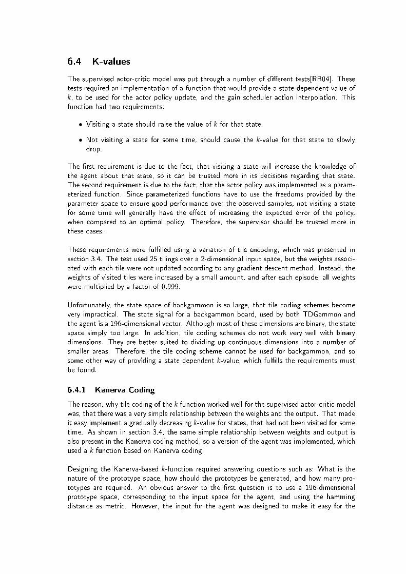
6.4 K-values

The supervised actor-critic model was put through a number of di�erent tests[RB04]. Thesetests required an implementation of a function that would provide a state-dependent value ofk, to be used for the actor policy update, and the gain scheduler action interpolation. Thisfunction had two requirements:

• Visiting a state should raise the value of k for that state.

• Not visiting a state for some time, should cause the k-value for that state to slowlydrop.

The �rst requirement is due to the fact, that visiting a state will increase the knowledge ofthe agent about that state, so it can be trusted more in its decisions regarding that state.The second requirement is due to the fact, that the actor policy was implemented as a param-eterized function. Since parameterized functions have to use the freedoms provided by theparameter space to ensure good performance over the observed samples, not visiting a statefor some time will generally have the e�ect of increasing the expected error of the policy,when compared to an optimal policy. Therefore, the supervisor should be trusted more inthese cases.

These requirements were ful�lled using a variation of tile encoding, which was presented insection 3.4. The test used 25 tilings over a 2-dimensional input space, but the weights associ-ated with each tile were not updated according to any gradient descent method. Instead, theweights of visited tiles were increased by a small amount, and after each episode, all weightswere multiplied by a factor of 0.999.

Unfortunately, the state space of backgammon is so large, that tile coding schemes becomevery impractical. The state signal for a backgammon board, used by both TDGammon andthe agent is a 196-dimensional vector. Although most of these dimensions are binary, the statespace simply too large. In addition, tile coding schemes do not work very well with binarydimensions. They are better suited to dividing up continuous dimensions into a number ofsmaller areas. Therefore, the tile coding scheme cannot be used for backgammon, and sosome other way of providing a state dependent k-value, which ful�lls the requirements mustbe found.

6.4.1 Kanerva Coding

The reason, why tile coding of the k function worked well for the supervised actor-critic modelwas, that there was a very simple relationship between the weights and the output. That madeit easy implement a gradually decreasing k-value for states, that had not been visited for sometime. As shown in section 3.4, the same simple relationship between weights and output isalso present in the Kanerva coding method, so a version of the agent was implemented, whichused a k function based on Kanerva coding.

Designing the Kanerva-based k-function required answering questions such as: What is thenature of the prototype space, how should the prototypes be generated, and how many pro-totypes are required. An obvious answer to the �rst question is to use a 196-dimensionalprototype space, corresponding to the input space for the agent, and using the hammingdistance as metric. However, the input for the agent was designed to make it easy for the

encoding interpretation000 0 checkers001 1 opponent checker010 2 opponent checkers011 3 or more opponent checkers100 1 agent checker101 2 agent checkers110 3 agent checkers111 4 or more agent checkers

Table 6.1: Kanerva prototype encoding

agent to recognize the non-linear e�ect of the input on the output. If the goal is simply to beable to distinguish the di�erent states from each other, then a more compact representationof the state, which encodes every point in only 3 bits, can be used. This is shown in table 6.1.Since a lot of the work in a Kanerva coding scheme goes into �nding the distance betweenstate representions, a more compact encoding will result in a performance speedup.

Generating prototypes is easy, when the di�erent dimensions are independent: For each di-mension in the prototype, generate a random value within the set of legal values for thatdimension. This approach cannot be used in backgammon, because the sets of legal valuesare not independent of each other. For instance, within the 24 dimensions correspondingto the points of the backgammon board, there cannot be 4 values of 111, since that wouldindicate a board with 16 or more agent checkers, which would be illegal. To overcome thisproblem, another method of generating the prototypes is used: A series of games is set upwith two players, that choose moves randomly. Any sample state from any one of these gameswill be a legal board, that can be translated into a legal prototype. It is a desirable propertyof the set of prototypes, that they cover a lot of di�erent states, i.e. the prototypes shouldnot be too similar. This means that the samples should not be from early parts of the game,where the states will be similar for all games, samples from the same game should not comefrom positions in the game sequence, that are too close, and since random games tend towardthe same type of positions, with most of the checkers in the opponents home table, samplesshould not come from too late in the game. Under these guidelines, every eigth of the �rst64 board states in a game were used to produce prototypes.

To answer the question of how many prototypes to generate, it is necessary to weigh theincreased resolution achieved by larger numbers of prototypes against the reduced compu-tational load from smaller numbers of prototypes. The problem is, that the time spentcomputing a k-value increases linearly with the number of prototypes, so a large number ofprototypes would make a single game take very long. In the end, samples were taken from1000 games, since that resulted in a reasonable game speed. That yields a rather smallnumber of prototypes compared to the size of the prototype space, so each prototype mustgeneralize to many other states in order to be useful. In order to achieve a high degreeof generalization, the set of prototypes activated by a state s is assumed to be the top 5%most similar prototypes, where similarity is the number of dimensions with the same encoding.

6.4.2 Neural Networks

Another way to implement the k function could be to use neural networks. After all, theyhave proved to be valuable in TDGammon, which also computes a function over backgammonboards, and a simple way to raise the value of visited states could be to provide a target of 1,and then do backpropagation. The problem arises with the requirement, that the state valueshould decrease for states, that have not been visited for a while. The naive way to implementthis would be to go over all non-visited states, training them with a target of 0. However, thenumber of unvisited states in a simple game is extremely large, so that is not a feasible solution.

What is the e�ect of not doing any e�ort to ful�ll the requirement to gradually decreasevalues? The frequently visited states will be trained to full autonomy for the agent, while thee�ect on the unvisited states will be more di�cult to predict. This may not be a problem,if none of the infrequently visited states are encountered during a normal game, which byde�nition is unlikely to happen. Therefore, it seems reasonable to implement the k-value byinitializing a neural network to produce a value close to 0 for all inputs, and then training theoutput for visited states on a target of 1. The network can be initialized to produce (closeto) 0 for all states by setting all connection weights to 0, and all neuron biases to -20.

6.4.3 State Independent Interpolation

When the requirement, that the k-value of infrequently visited states should decrease, isdropped, the values for all states will rise toward 1 with varying speeds. For the set of statesfrequently visited states during a normal game, those speeds may be roughly similar. Thissuggests a further simpli�cation: To simply disregard the speci�c state, and only vary thek-value as a non-decreasing function of the number of training episodes. A simple examplecould be a trapezoid function, that is zero for all training episodes below some threshold,rising linearly to 1 between that threshold and another, and 1 for training episodes above thesecond threshold, as shown in �gure 6.2.

Figure 6.2: A trapezoid function

Such a function raises an interesting question: What should be the positions of the left andright thresholds? Looking at the performance of the baseline shown in chapter 5, it seemsclear, that the agent should be in full control, when the performance of the agent trainedwithout supervision reaches that of the supervisor. Otherwise, the supervisor may actuallyhurt the combined performance. In this case, the performance of the baseline, which is justthe agent trained without supervision, shows, that the right threshold should be at roughlyat 5000 training episodes. However, in some situations, there may not be an estimate of theunsupervised agent performance. For the left threshold, it is not completely clear, whether itis better to leave the supervisor in total control for a while, or whether control should startto transfer to the agent immediately.

6.5 Conclusion

In summary of this chapter:

• The agent is implemented as a neural network structure.

• The combined action is either the agent or the supervisor action, partially dependenton k.

• The network is trained on a weighted sum of the reinforcement target and the supervisortarget, with the weights dependent on k.

• 3 di�erent k function have been proposed: Kanerva based, neural network based andtrapezoid.

It remains to choose a few parameters:

• Value of λ in TD(λ): 0. [Tes92] states, that performance was similar for values in therange [0.0 , 0.7], and a value of 0 is computationally simpler.

• Number of hidden units: 80. This is the same as some versions of TDGammon.

• Learning rate: 0.1. This is the same as in TDGammon[Tes92].

There are now 3 slightly di�erent designs of supervised reinforcement learning in backgammonready to be tested.

Chapter 7

Test

7.1 Introduction

The testing process was de�ned in chapter 5. Brie�y, each agent is to be trained for 100000training episodes1. The performance of the agent is then to be measured every 1000 trainingepisodes, and compared to the baseline.

7.2 Test Results

The results for the 3 designs are shown in �gures 7.1, 7.2 and 7.3. It seems clear, that theagents using interpolation based on either Kanerva coding or neural networks do not improveupon the performance of the supervisor. In fact, the results seem to indicate, that the interpo-lation for both these agents must be heavily favoring the supervisor throughout the training.There are a couple of reasons, why this might be so. For the neural network interpolation, thenetwork was initialized to a value of nearly 0 for all states by setting all weights to 0, and thebias to -20. It is not normal to initialize any weights or biases in a neural network with sucha numerically large value, since the gradient for the sigmoid activation function, evaluatedat -20 is very small, and thus during training, where the weight update is dependent on thegradient, the weight increments were too small to have any e�ect during the course of the100000 training episodes.

For the Kanerva-based interpolation, a could be a problem, that the number of prototypes,which was approximately 8000, were not su�cient to capture the complexity of the statespace. Therefore, with the decision of always activating the closest 5% of the prototypes,prototypes would be randomly activated. With the random activation, the weight increasesdue to state visits would spread evenly among all the protypes. Since none of the prototypeswould consistently receive weight increases, the weight decreasing factor of 0.999, that wasapplied to all weights, might have been enough to keep all of the prototype weights at a lowenough level, that the supervisor could dominate the interpolation.

In contrast to the both the Kanerva-based and neural network-based interpolation, the simpletrapezoid interpolation worked reasonably well. It was able to avoid the initial bad performanceof the baseline, although the performance did fall a bit before the learning really started towork. Another problem is, that although the performance was initially better than the baseline,

1interpreted here as equivalent to 50000 self-play games, since the agent will be trained on both thewinning and losing board sequence.

41

Figure 7.1: Performance of supervised reinforcement learning using Kanerva-based interpola-tion

Figure 7.2: Performance of supervised reinforcement learning using neural network-based inter-polation

Figure 7.3: Performance of supervised reinforcement learning using trapezoid interpolation, leftthreshold 0, right threshold 5000

the baseline performance overtook the agent performance at around 45000 training episodes.This is not easily explainable, since at that point the agent should be fully autonomous, andtherefore use the same learning mechanism as the baseline. A �nal problem with the state-independent trapezoid interpolation is, that it is not clear how to choose the shape of theinterpolation function. The e�ect of choosing a very di�erent interpolation function is shownon �gure 7.4, which also uses a trapezoid interpolation, but with the right threshold movedto 50000 instead of 5000 training episodes. This interpolation ensures, that the initial dropin performance seen in the shorter trapezoid interpolation does not occur. The price paid forthis is that the baseline overtakes the agent much earlier, and that the agent stays at thesupervisor performance much longer.

Figure 7.4: Performance of supervised reinforcement learning using trapezoid interpolation, leftthreshold 0, right threshold 5000

7.3 Conclusion

This chapter has presented the results of testing the agents designed previously. It has shown,that it is possible to apply supervision to the reinforcement learning process in order to avoidthe initial period of bad performance. In addition, it has shown the importance of increasingagent autonomy at the right pace. If the agent has control too soon, the performance maydrop initially, since the supervisor has not had enough time to teach. If the supervisor remainsin control for too long, performance will su�er in the longer term, since the agent is notallowed to learn from experience, and thereby surpass the performance of its supervisor.

Some possible improvements for the agents suggest themselves:

• The neural network interpolation could probably be improved by also setting the biasto 0. That would initialize the interpolation to 0.5 for all states. Then output in therange [0.5 - 1] could be mapped to [0 - 1]. In this way the network would be muchmore responsive to training.

• If another supervisor was chosen, with higher performance, it may be that a trapezoidinterpolation function could be found, that allowed the agent enough time to train toavoid the initial performance drop, and at the same time released control to the agentquickly enough, that the baseline did not overtake it.

Chapter 8

Conclusion

The backgammon domain is very well suited to pure reinforcement learning: It has a naturalformulation as a reinforcement learning task, it has a built-in exploration mechanism, and cantake advantage of the presence of afterstates to estimate a state-value function instead of themore complicated action-value function. As a result, several very good backgammon players,such as TDGammon have been implemented using reinforcement learning.

Reinforcement learning has the drawback, that it may take a long time to reach an good levelof performance, and that when the training starts, the performance may be unacceptably low.This report has developed a framework for supervised reinforcement learning in the backgam-mon domain, based on an interpolation of the agent and supervisor, in order to reduce thosedrawbacks.

The backgammon domain is not as perfect a �t for supervised reinforcement learning usingthe interpolation model, as it is for pure reinforcement learning. This is primarily due to twoaspects of the domain:

1. The input has a high dimensionality. This has meant, that the interpolation functionneeded to be adapted.

2. The actions are discrete and unordered. This has meant that the learning functionneeded to be adapted.

Adapting the interpolation function was made easier by the realization, that in the domainof backgammon, there is a relatively small part of the state space, that can reasonably beexpected to occur in a normal game. For these states, the agent should be steadily moreautonomous, since these are the states, that the agent gets to know well. Using a kind ofcircular logic, since these are the states, that are likely to be seen in a normal game, the agentshould be granted more autonomy for all states it encounters. This simpli�cation allowed theimplementation of 3 di�erent interpolation functions. Both the function based on Kanervacoding, and the function based on neural networks did not do so well. Their performanceremained at the level of the supervisor, and performed worse than the baseline for most ofthe test. This is probably for di�erent reasons. The Kanerva function only had around 8000prototypes, and given the complexity of the input space, this was probably not enough. Theneural network function may have been initialized so that it required more training than in-cluded in the test to reach autonomy for the agent. In contrast, the trapezoid interpolationfunction removed the initial period of bad performance, while still being able to improve as a

45

result of the reinforcement learning. However, a negative e�ect of the supervision seems tobe a slower overall learning rate, and a bad choice of thresholds of the interpolation functioncan reduce performance.

Adapting the learning function resulted in the requirement that the supervisor should have thesame type of output as the learner. This has also worked well, but is a quite harsh restrictionon the supervisor. The framework presented here would be much more useful, if an arbitrarysupervisor could be used.

Going forward from here, there are some simple modi�cations, that might increase perfor-mance:

• Using a supervisor that plays at a higher level may yield a consistently better performancethan the baseline, until they both settle, instead of the baseline just catching up, whenit starts to improve.

• Using a constant learning rate, as TDGammon does is not recommended in the theory.Using a diminishing learning rate might allow the performance to stabilize at a higherlevel, although the performance might rise slower.

These modi�cations are aimed at increasing performance, which is very nice, but the mostbene�t would come from increasing the scope of the framework. To achieve this goal, it isnecessary to address one or both of the following challenges.

• Find some way to remove the supervisor output restriction.

• Find a heuristic to determine the best shape of the stateless interpolation function, orimplement a good state-based interpolation function.

Appendices

47

Appendix A

N-ply Search

This chapter describes the n-ply search, that has been implemented in the backgammonframework. N-ply search can be thought of as mentally playing ahead of the game, insteadof just looking at the current board. A ply is a single turn for one of the players, and the'n' in n-ply refers to how many plies the search should look ahead. The branching factor forbackgammon is quite high, so it is usually not feasible to look ahead more than 2 or 3 plies.The search gives rise to a tree of di�erent boards: A single board expands to more boards,and each of these boards expand to even more boards. The 'n' of n-ply can therefore also bethought of as the depth of this search tree.

As an example, consider the expansion to depth 1 associated with 1-ply search, in a gamebetween players A and B. In order for player A to obtain the score of one of the possiblemoves, recall that such a move represents the state of the backgammon game, after it hasbeen player A has �nished his turn, if he chooses to make that move. So now it is playerB's turn to move. Since player A doesn't know, which dice B will roll, he has to try out allcombinations of them. There are 21 di�erent combinations (since permutations give rise tothe same possible moves for the opponent), and each of these combinations present B witha choice of which move to make, using those dice. player A doesn't know how B choosesmoves, so he has to try to guess. The guess is, that B will choose the move, that A wouldchoose, without looking ahead, only with the sides reversed: A guesses that B chooses themove, that A thinks is the worst move. So now A has for each dice combination a move, thathe thinks, that B will make using those dice, and has assigned a value to each of those moves.Thus, the original move is associated with 21 di�erent scores, which can be aggregated intothe single 1-ply search score. However, these 21 boards are not all equally likely to occur.Speci�cally, dice combinations (and their associated scores) that are not doubles, are twiceas likely to occur as dice combinations, that are doubles. Therefore, the 1-ply search score ofthe original board is a weighted average of the expanded board scores.

Deeper expansion is easy. For instance, boards can be expanded to depth 2 by further expan-sion of each of the 21 boards selected by the opponent, for a total of 441 weighted scores.The weights are modi�ed, so that scores obtained from two successive double rolls are givenweight 1, scores obtained from a combination of double and non-double rolls are given weight2, and scores obtained from two successive non-double rolls are given weight 4. It is worthnoting, that the value function used for choosing boards at each step of the expansion isthe same, regardless of search depth or current expansion step. This has the e�ect that theoriginal moves are evaluated using an n-depth search, but the expansion mechanism itself

49

uses only zero-depth search, for each expansion step. . Obviously, it is not possible to usen-depth search for all expansion steps, because then the search would never �nish (or at leastnot until the end of the game had been reached, which would take an exceedingly long time,considering that each ply adds a branching factor of 21), but it is conceivable that expansionstep 1 used (n-1)-ply search, expansion step 2 used (n-2)-ply search and so on. This is notimplemented for performance reasons.

Finally, once each of the possible original moves of A have a score, it is time to choose thebest move. This is dependent on the search depth. The score for each move represents theprobable value of choosing that move as the next move, as perceived by the player, who, atthe n'th expansion step, supplied the weighted scores, which have been aggregated to formthe �nal move score. Therefore, if the depth is even, the current player has supplied thescores, and the best move is the move with the highest score, and if the score is odd, theopponent has supplied the score, and therefore the best move is the move with the lowest score.

This n-ply search scheme was implemented after a design by Gerald Tesauro, outlined in[Tes02]. Note, that the semantics of this report di�er from those of Tesauro, in that whathe describes as 1-ply search, is equivalent to 0-ply search in the context of this thesis. Usingn-ply search is a very good way to improve the performance of an agent, after it has beentrained. It is not good to evaluate states by any other search than 0-ply search, since usingjust 1-ply search will cause an agent to spend roughly 400 times more time on choosing amove. However, once an agent has been trained, its performance can be increased quitedramatically by using 1-ply search. As an example, the test baseline evaluated after 100000training episodes, using 0-ply search won 55.7 percent of the games in a 5000 game trial,while the same baseline using 1-ply search won 65,8 percent of the games in a 400 gametrial. Using 2-ply search is usually only practical for games versus humans, since just makinga single move may take on the order of 10 seconds, according to [Tes02]. The tests in thisthesis were conducted using only 0-ply search.

Bibliography

[Ben96] Hamid Benbrahim. Biped dynamic walking using reinforcement learning. PhDthesis, Durham, NH, USA, 1996. Director-Miller,III, W. Thomas.

[CB96] Robert Crites and Andrew Barto. Improving elevator performance using reinforce-ment learning. In Advances in Neural Information Processing Systems 8, pages1017�1023. MIT Press, 1996.

[Cet06] Victor Uc Cetina. A multiagent architecture for concurrent reinforcement learning.In ESANN, pages 107�112, 2006.

[Cet08] Victor Uc Cetina. Autonomous agent learning using an actor-critic algorithm andbehavior models. In AAMAS '08: Proceedings of the 7th international joint confer-ence on Autonomous agents and multiagent systems, pages 1353�1356, Richland,SC, 2008. International Foundation for Autonomous Agents and Multiagent Sys-tems.

[Hei04] Mikael Heinze. Intelligent game agents, developing an adaptive fuzzy controlledbackgammon agent. Master's thesis, Aalborg University Esbjerg, Esbjerg, Den-mark, 2004.

[KAK+95] Hiroaki Kitano, Minoru Asada, Yasuo Kuniyoshi, Itsuki Noda, and Eiichi Osawa.Robocup: The robot world cup initiative, 1995.

[Kan93] Pentti Kanerva. Sparse distributed memory and related models. In AssociativeNeural Memories, pages 50�76. Oxford University Press, 1993.

[KH01] Kostas Kostiadis and Huosheng Hu. Kabage-rl: Kanerva-based generalisation andreinforcement learning for possession football. In In Proceedings of the IEEE/RSJInternational Conference on Intelligent Robots and Systems (IROS, 2001.

[McC59] John McCarthy. Programs with common sense. In Proceedings of the TeddingtonConference on the Mechanization of Thought Processes, pages 75�91, London,1959. Her Majesty's Stationary O�ce.

[Mit97] Tom M. Mitchell. Machine Learning. McGraw-Hill, New York, 1997.

[MSK96] Richard Maclin, Jude W. Shavlik, and Pack Kaelbling. Creating advice-takingreinforcement learners. In Machine Learning, pages 251�281, 1996.

[Neu08] Neurondotnet, 2008.

[Nie06] Niels Nygaard Nielsen. Intelligent game agents, improving a fuzzy controller basedbackgammon player. Master's thesis, Aalborg University Esbjerg, Esbjerg, Den-mark, 2006.

51

[PB98] Jordan B. Pollack and Alan D. Blair. Co-evolution in the successful learning ofbackgammon strategy. In Machine Learning, pages 225�240, 1998.

[RB04] Michael T. Rosenstein and Andrew G. Barto. Supervised actor-critic reinforcementlearning. In Learning and Approximate Dynamic Programming: Scaling Up to theReal World. John Wiley & Sons, 2004.

[SALL00] Scott Sanner Sanner, John R. Anderson, Christian Lebiere, and Marsha Lovett.Achieving e�cient and cognitively plausible learning in backgammon. In In Pro-ceedings of the Seventeenth International Conference on Machine Learning (ICML-2000, pages 823�830. Morgan Kaufmann, 2000.

[Sam95] A. L. Samuel. Some studies in machine learning using the game of checkers. pages71�105, 1995.

[SB97] Satinder Singh and Dimitri Bertsekas. Reinforcement learning for dynamic channelallocation in cellular telephone systems. In Michael C. Mozer, Michael I. Jordan,and Thomas Petsche, editors, Advances in Neural Information Processing Systems,volume 9, page 974. The MIT Press, 1997.

[SB98] Richard S. Sutton and Andrew G. Barto. Reinforcement Learning: An Introduction(Adaptive Computation and Machine Learning). The MIT Press, March 1998.

[Sut88] Richard S. Sutton. Learning to predict by the methods of temporal di�erences.Machine Learning, 3:9�44, 1988.

[Sut96] Richard S. Sutton. Generalization in reinforcement learning: Successful examplesusing sparse coarse coding. In Advances in Neural Information Processing Systems8, volume 8, pages 1038�1044, 1996.

[SW93] Richard S. Sutton and Steven D. Whitehead. Online learning with random repre-sentations. In In Proceedings of the Tenth International Conference on MachineLearning, pages 314�321. Morgan Kaufmann, 1993.

[Tes92] Gerald Tesauro. Practical issues in temporal di�erence learning. In MachineLearning, pages 257�277, 1992.

[Tes95] Gerald Tesauro. Temporal di�erence learning and td-gammon. Commun. ACM,38(3):58�68, 1995.

[Tes98] Gerald Tesauro. Comments on �co-evolution in the successful learning of backgam-mon strategy�. Mach. Learn., 32(3):241�243, 1998.

[Tes02] Gerald Tesauro. Programming backgammon using self-teaching neural nets. Artif.Intell., 134(1-2):181�199, 2002.

[Tes08] Gerry Tesauro. Benchmark player, January 2008.

[UC91] Paul E. Utgo� and Je�ery A. Clouse. Two kinds of training information for eval-uation function learning. In In Proceedings of the Ninth Annual Conference onArti�cial Intelligence, pages 596�600. Morgan Kaufmann, 1991.