dynamic soil properties and liquefaction - ikbooks.com dynamic soil properties and ... varies from...
TRANSCRIPT
Dynamic Soil Properties and Liquefaction
CHAPTER 2
2.1 OVERVIEW
Several problems in engineering practice require knowledge of the dynamic soil properties and liquefaction. Generally, problems related to foundations and retaining structures subjected to dynamic loads problems are divided into either a small strain amplitude or large strain amplitude response. Structures during earthquakes are able to tolerate large strain levels. The major soil properties that are required to analyze the behaviour of a structure subjected to dynamic loads are: 1. Dynamic Young’s modulus (E) and dynamic shear modulus (G) 2. Poisson’s ratio (m) 3. Damping usually in terms of damping ratio (x) 4. Liquefaction parameters like cyclic shearing stress ratio and cyclic deformation. Values of E and G are dependent on confining pressure and strain level. There are various tests available for determining E and G. It has been observed that in general Poisson’s ratio (m) varies from 0.25 and 0.35 for cohesionless soils and from about 0.35 and 0.45 for cohesive soils. Responses of structure-foundation-soil systems are not sensitive to the variations in the value of m. Damping ratio of the medium may be obtained by performing dynamic tests. Methods are available to obtain cyclic stress ratio for examining the liquefaction potential. Discussions on all these aspects have been included in this chapter.
2.2 RESONANT COLUMN TEST
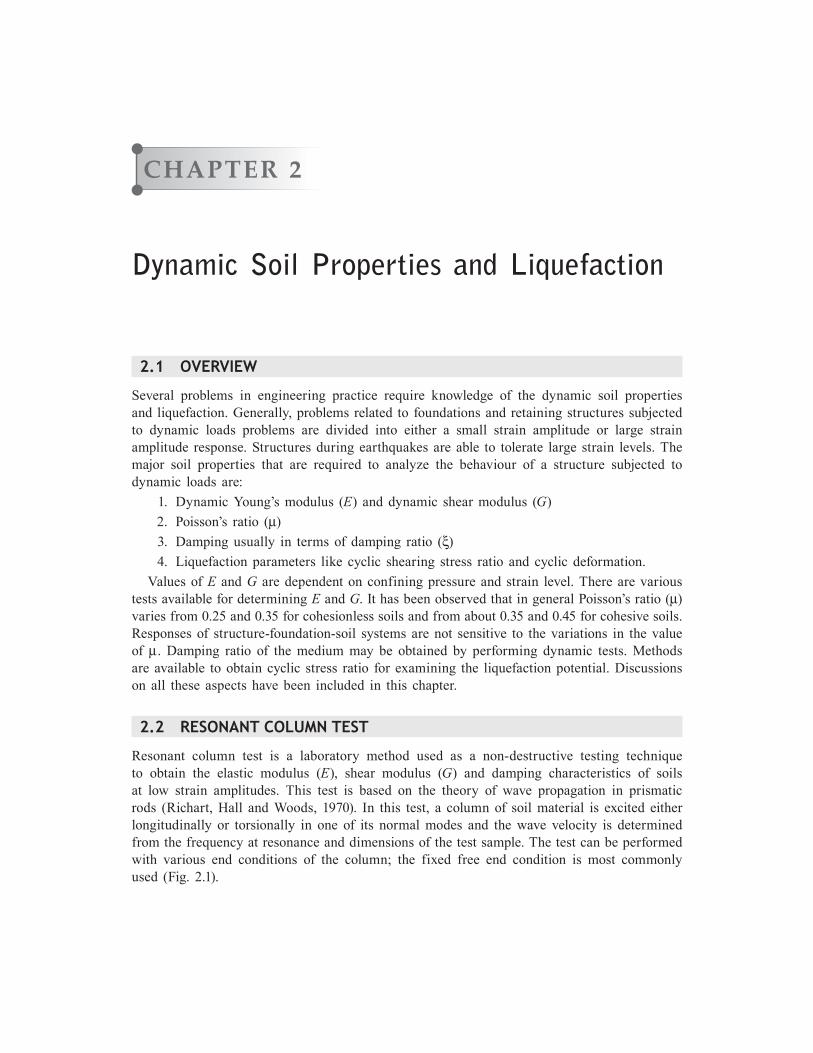
Resonant column test is a laboratory method used as a non-destructive testing technique to obtain the elastic modulus (E), shear modulus (G) and damping characteristics of soils at low strain amplitudes. This test is based on the theory of wave propagation in prismatic rods (Richart, Hall and Woods, 1970). In this test, a column of soil material is excited either longitudinally or torsionally in one of its normal modes and the wave velocity is determined from the frequency at resonance and dimensions of the test sample. The test can be performed with various end conditions of the column; the fixed free end condition is most commonly used (Fig. 2.1).
14 Foundations and Retaining Structures
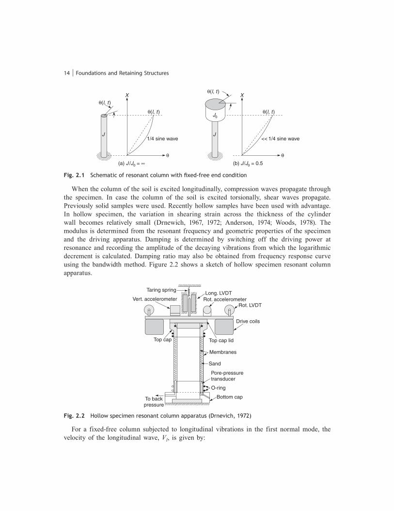
When the column of the soil is excited longitudinally, compression waves propagate through the specimen. In case the column of the soil is excited torsionally, shear waves propagate. Previously solid samples were used. Recently hollow samples have been used with advantage. In hollow specimen, the variation in shearing strain across the thickness of the cylinder wall becomes relatively small (Drnewich, 1967, 1972; Anderson, 1974; Woods, 1978). The modulus is determined from the resonant frequency and geometric properties of the specimen and the driving apparatus. Damping is determined by switching off the driving power at resonance and recording the amplitude of the decaying vibrations from which the logarithmic decrement is calculated. Damping ratio may also be obtained from frequency response curve using the bandwidth method. Figure 2.2 shows a sketch of hollow specimen resonant column apparatus.
Fig. 2.1 Schematic of resonant column with fi xed-free end condition
q( , )l t
J
X
q
1/4 sine wave
q( , )l t
(a) / =J J0 •
q( , )l t
J
X
q
<< 1/4 sine wave
q( , )l t
(b) / = 0.5J J0
J0
Fig. 2.2 Hollow specimen resonant column apparatus (Drnevich, 1972)
Rot. LVDTRot. accelerometerLong. LVDT
Vert. accelerometer
Taring spring
Drive coils
Top cap lid
Membranes
Sand
Pore-pressuretransducer
O-ring
Bottom capTo backpressure
Top cap
For a fixed-free column subjected to longitudinal vibrations in the first normal mode, the velocity of the longitudinal wave, Vl, is given by:
Dynamic Soil Properties and Liquefaction 15
W ___ Wo =
wnl h ____ Vl tan ( wnl h ____ Vl
) ...(2.1)
where, W = weight of specimen, Wo = weight of loading system, wnl = natural frequency of first natural mode, and h = height of the specimen. If the loading system is massless (i.e., Wo = 0), Eq. (2.1) reduces to;
Vl = 2wnlh _____ p ...(2.2a)
or, Vl = 4fnlh ...(2.2b)fnl is the natural frequency in cps. Knowing the value of Vl, value of dynamic Young’s modulus (E) is obtained by:
E = rVl2 ...(2.3)
where, r = mass density of soil specimen. For solid specimen,
r = 4W ______ p d2hg
= g __ g ...(2.4a)
For hollow specimen,
r = 4W ____________ p(do
2 – di2) hg
= g __ g ...(2.4b)
where, W = total weight of specimen, d = diameter of solid specimen, do = outer diameter of hollow specimen, di = inner diameter of hollow specimen, g = acceleration due to gravity, and g = unit weight of soil at which specimen is prepared. If the fixed-free column is excited torsionally, the shear wave velocity (Vs) is given by:
I __ Io =
wnsh ____ Vs tan ( wnsh ____ Vs
) ...(2.5)
where, I = mass polar moment of inertial of the specimen, and Io = mass polar moment of inertial of the torsional loading system connected to the top of the specimen.
16 Foundations and Retaining Structures
If the loading system is massless (i.e., Io = 0), Eq. (2.5) reduces to:
Vs = 2wnsh _____ p ...(2.6a)
or, Vs = 4fnsh ...(2.6b)
Knowing the value of Vs, value of dynamic shear modulus (G) is obtained by:
G = rVs2 ...(2.7)
Knowing the values of E and G, Poisson’s ratio (m) may be obtained using the following relation,
G = E _______ 2(1 + m) ...(2.8a)
or, m = E ___ 2G – 1 ...(2.8b)
2.3 CYCLIC PLATE LOAD TEST
The cyclic plate load test is a modified version of the standard plate load test. This test facilitates in separating the elastic (recoverable) part of deformation from the total settlement which in turn is related to the Young’s modulus of the soil. The cyclic plate load test is performed in a test pit dug upto the proposed base level of foundation. The equipment is same as used in conventional plate load test. Circular or square bearing plates of mild steel not less than 25 mm thickness and varying in size from 300 to 750 mm with chequered or grooved bottom are used. The test pit should be at least five times the width of the plate. The equipment is assembled according to the details given in IS 1988-1982. A typical set-up is shown in Fig. 2.3. To commence the test, a seating pressure of about 7 kPa is first applied to the plate. It is then removed, dial gauges are set to read zero. Load is then applied in equal cumulative increments of not more than 100 kPa or of not more than one-fifth of the load corresponding to estimated allowable bearing pressure. In cyclic plate load test, each incremental load is maintained constant till the settlement of the plate is complete. The load is then released to zero and the plate is allowed to rebound. The reading of final settlement is taken. The load is then increased to next higher magnitude of loading and maintained constant till the settlement is complete, which again is recorded. The load is then reduced to zero and the settlement reading taken. The next increment of load is then applied. The cycles of unloading and reloading are continued till the required final load is reached. The data obtained from a cyclic plate load test is shown in Fig. 2.4(a). From this data, the load intensity versus elastic rebound is plotted as shown in Fig. 2.4(b), and the slope of the line is coefficient of elastic uniform compression.
Cu = p __ Se (kN/m3) ...(2.9)

Dynamic Soil Properties and Liquefaction 17
Sand bags to give areaction of 500 kN
R.S.J. 300 mm × 150 mm
1.5 m
1.0 m0.60 m
1.0 m 0.60 m
Channel
Foundation level
Plate 300 mm × 300 mm
Sectional elevation
Proving ring
Wooden sleeper2 m × 0.30 m × 0.15 m
2 nos. on either side
R.S.J. 150 mm × 750 mm × 300 mm
1.5 m
100 mm
3 nos R.S.J. 300 mm × 150 mm at 400 mm c/ctop row of joists not shown in plan
Fig. 2.3 A typical set-up for cyclic plate load test
p1
Se2
Se3
Se4
Se5
Set
tlem
ent,
S
p2 p3 p4 p5
Load
inte
nsity
,p
Se
p
Elastic rebound, Se
(b)(a)
Load intensity, p
Fig. 2.4 (a) Load intensity versus settlement curve in a cyclic plate load test, (b) Load intensity versus elastic rebound plot from cyclic plate load test
18 Foundations and Retaining Structures
where, p = load intensity in kN/m2, and Se = elastic rebound corresponding to p in m. For a square rigid plate of area A in m2, on an elastic medium subjected to vertical load, Cu is related with E by the relation given below:
Cu = 1.08 E _______ (1 – m2)
1 ___ ÷
__ A ...(2.10)
Value of shear modulus G may be obtained using relation (2.8a) once the value of E is determined using (2.10).
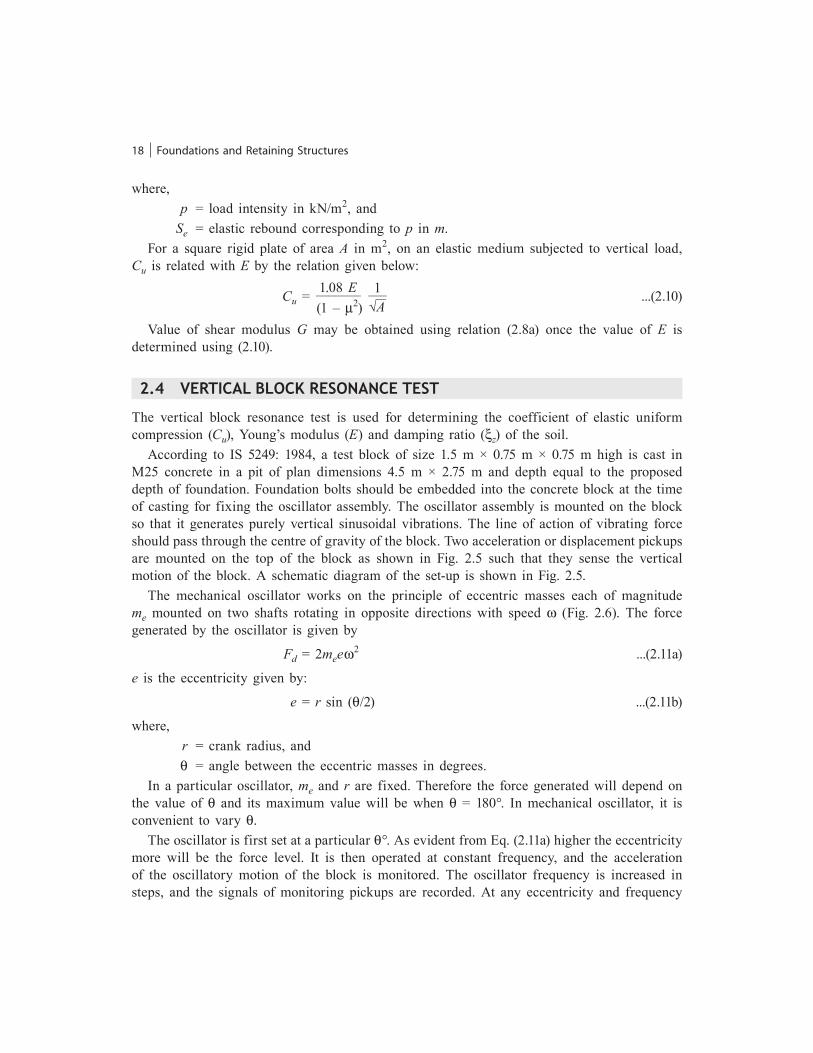
2.4 VERTICAL BLOCK RESONANCE TEST
The vertical block resonance test is used for determining the coefficient of elastic uniform compression (Cu), Young’s modulus (E) and damping ratio (xz) of the soil. According to IS 5249: 1984, a test block of size 1.5 m × 0.75 m × 0.75 m high is cast in M25 concrete in a pit of plan dimensions 4.5 m × 2.75 m and depth equal to the proposed depth of foundation. Foundation bolts should be embedded into the concrete block at the time of casting for fixing the oscillator assembly. The oscillator assembly is mounted on the block so that it generates purely vertical sinusoidal vibrations. The line of action of vibrating force should pass through the centre of gravity of the block. Two acceleration or displacement pickups are mounted on the top of the block as shown in Fig. 2.5 such that they sense the vertical motion of the block. A schematic diagram of the set-up is shown in Fig. 2.5. The mechanical oscillator works on the principle of eccentric masses each of magnitude me mounted on two shafts rotating in opposite directions with speed w (Fig. 2.6). The force generated by the oscillator is given by
Fd = 2meew2 ...(2.11a)
e is the eccentricity given by:
e = r sin (q/2) ...(2.11b)
where, r = crank radius, and q = angle between the eccentric masses in degrees. In a particular oscillator, me and r are fixed. Therefore the force generated will depend on the value of q and its maximum value will be when q = 180°. In mechanical oscillator, it is convenient to vary q. The oscillator is first set at a particular q°. As evident from Eq. (2.11a) higher the eccentricity more will be the force level. It is then operated at constant frequency, and the acceleration of the oscillatory motion of the block is monitored. The oscillator frequency is increased in steps, and the signals of monitoring pickups are recorded. At any eccentricity and frequency
20 Foundations and Retaining Structures
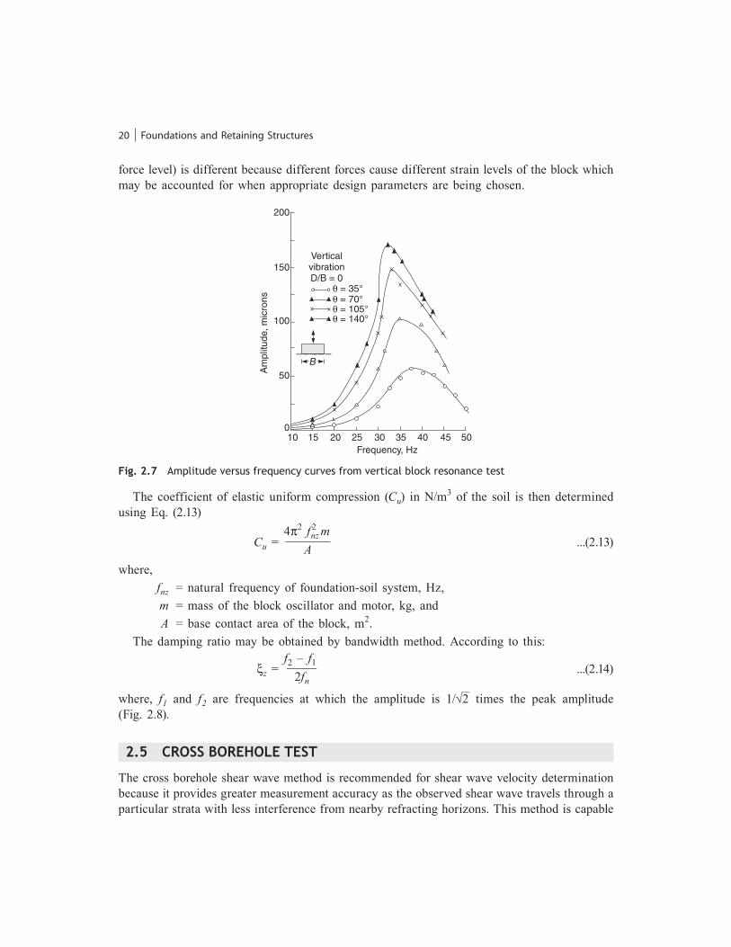
force level) is different because different forces cause different strain levels of the block which may be accounted for when appropriate design parameters are being chosen.
Fig. 2.7 Amplitude versus frequency curves from vertical block resonance test
15
200
150
100
50
010 20 25 30 35 40 45 50
Am
plitu
de, m
icro
ns
B
q = 35°q = 70°q = 105°q = 140°
VerticalvibrationD/B = 0
Frequency, Hz
The coefficient of elastic uniform compression (Cu) in N/m3 of the soil is then determined using Eq. (2.13)
Cu = 4p2 f 2nz m ________ A ...(2.13)
where, fnz = natural frequency of foundation-soil system, Hz, m = mass of the block oscillator and motor, kg, and A = base contact area of the block, m2. The damping ratio may be obtained by bandwidth method. According to this:
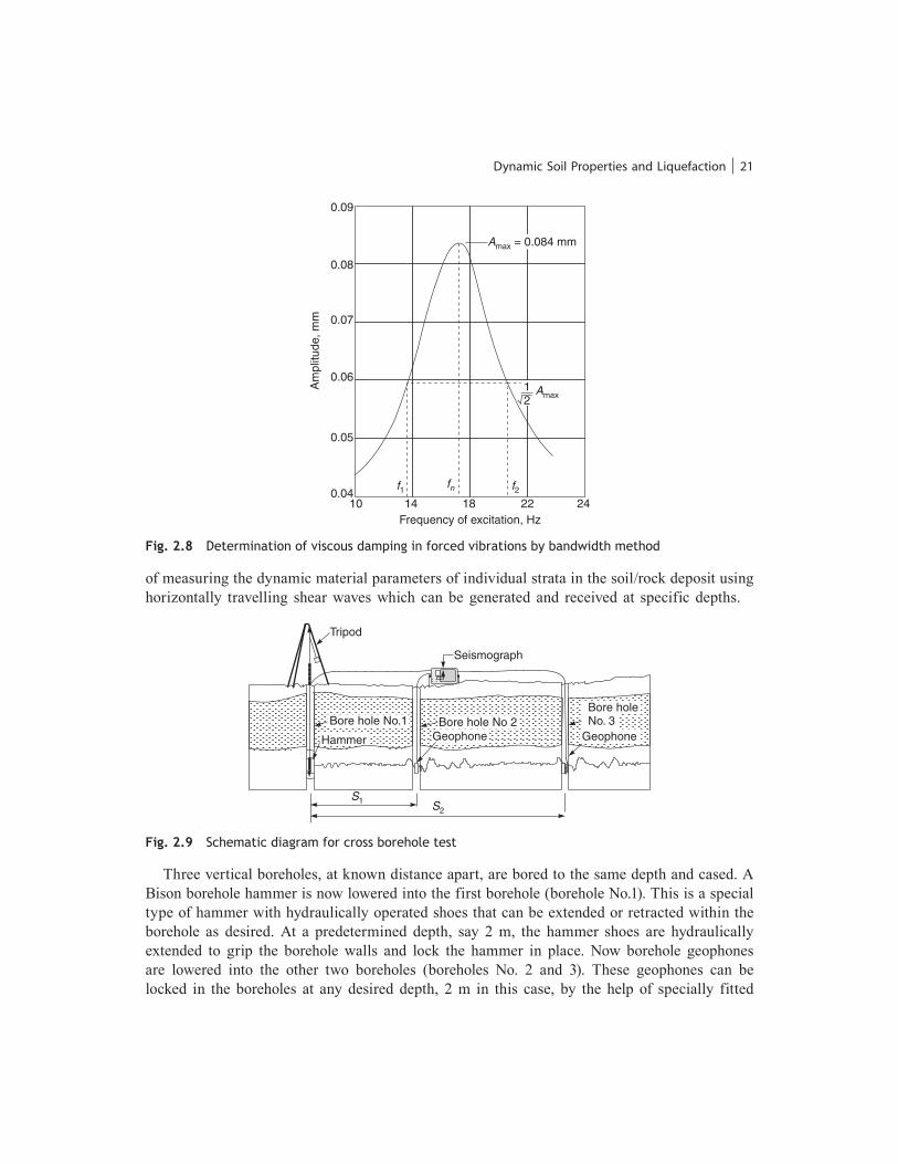
xz = f2 – f1 _____ 2fn
...(2.14)
where, f1 and f2 are frequencies at which the amplitude is 1/ ÷ __
2 times the peak amplitude (Fig. 2.8).
2.5 CROSS BOREHOLE TEST
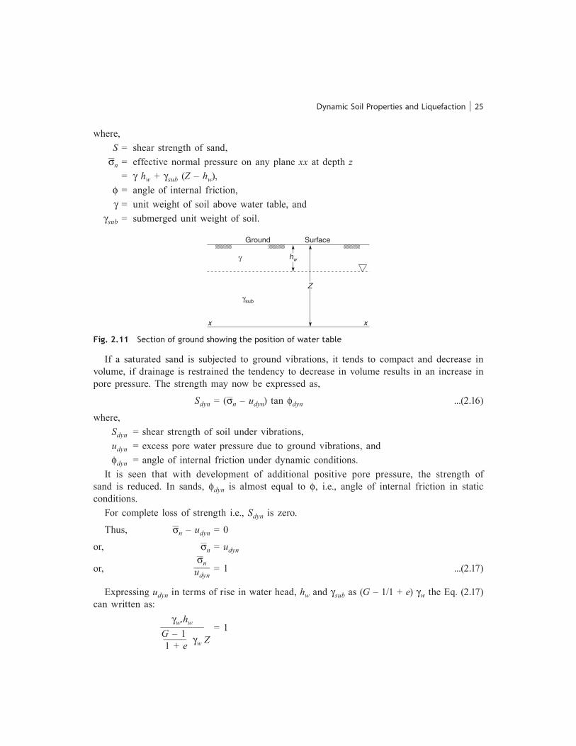
The cross borehole shear wave method is recommended for shear wave velocity determination because it provides greater measurement accuracy as the observed shear wave travels through a particular strata with less interference from nearby refracting horizons. This method is capable
Dynamic Soil Properties and Liquefaction 21
of measuring the dynamic material parameters of individual strata in the soil/rock deposit using horizontally travelling shear waves which can be generated and received at specific depths.
10 14 18 22 24
f1 fn f2
Frequency of excitation, Hz
12
Amax
0.09
0.08
0.07
0.06
0.05
0.04
Am
plitu
de, m
m
Amax = 0.084 mm
Fig. 2.8 Determination of viscous damping in forced vibrations by bandwidth method
Tripod
GeophoneBore hole No 2Bore hole No.1
Hammer
Bore holeNo. 3
Geophone
Seismograph
S2
S1
Fig. 2.9 Schematic diagram for cross borehole test
Three vertical boreholes, at known distance apart, are bored to the same depth and cased. A Bison borehole hammer is now lowered into the first borehole (borehole No.1). This is a special type of hammer with hydraulically operated shoes that can be extended or retracted within the borehole as desired. At a predetermined depth, say 2 m, the hammer shoes are hydraulically extended to grip the borehole walls and lock the hammer in place. Now borehole geophones are lowered into the other two boreholes (boreholes No. 2 and 3). These geophones can be locked in the boreholes at any desired depth, 2 m in this case, by the help of specially fitted

22 Foundations and Retaining Structures
rubber bladders, which can be inflated pneumatically. The electrical signals from the borehole hammer and geophones are fed into a Bison seismograph. A schematic diagram for the cross borehole test is shown in Fig. 2.9. Having locked the borehole hammer and geophones at the same desired depth, 2 m in this case, the seismograph is switched on. A shear wave is now generated in the first borehole by operating the hammer. This activates a timer switch in the seismograph and the shear waveform arrivals at the borehole geophones are displayed on the video screen of the seismograph. The waveforms are now analyzed and the exact arrival time of the shear waves are calculated, for the borehole locations (boreholes no. 2 and 3) and depth (2 m in this case). The hydraulically operated hammer shoes are now retracted and the hammer lowered to its next depth say 4 m, and again locked in position by extending the shoes. Similarly, the borehole geophones are now lowered and locked at the same new depth of 4 m by deflating and then again inflating the rubber bladders. The shear wave is now generated and the arrival times computed as discussed above for the 2 m depth case. This process is repeated for as many depths as planned to obtain a shear wave profile for the location under consideration. Having obtained the shear wave travel time, Ts1 and Ts2, for the known distances between the boreholes (S1 and S2, Fig. 2.9), the shear wave velocity (Vs) for a particular depth was obtained as:
Vs = S1/Ts1 = S2/Ts2 ...(2.14a)
Specifi cations for the Tests
(a) A set of 3 boreholes laid out along a line are needed at each location. The spacing between the boreholes depends on the data of borelogs from the site. The boreholes should be cleaned and cased with PVC casing pipes and should have an internal diameter of 85 mm to 90 mm. The PVC casing pipes should be able to withstand pressures upto 1000 kN/m2 (IS 4568 PVC pipes). The cased boreholes should be made upto the required depth.
(b) The boreholes need to be plugged at the bottom and the water inside the cased borehole pumped out.
(c) It is required to have the boreholes made of the same diameter as the PVC casing pipes. In case boreholes of 150 mm diameter are first made and then the PVC casings of 85 mm to 90 mm internal diameter are installed in them, the annular space between the 150 mm diameter hole and the PVC casing is to be backfilled with a clean sand slurry. The backfilling has to be done properly as if there are any voids this will affect the resultant shear wave velocity. The shear wave cannot travel through voids.
2.6 SASW TEST
The Spectral Analysis of Surface Waves (SASW) is a new seismic method for quick and economical determination of shear wave velocity (in situ). It utilizes the dispersive nature
Dynamic Soil Properties and Liquefaction 25
where, S = shear strength of sand,
__ s n = effective normal pressure on any plane xx at depth z
= g hw + gsub (Z – hw), f = angle of internal friction, g = unit weight of soil above water table, and gsub = submerged unit weight of soil.
gsub
Ground
Z
hw
x x
g
Surface
Fig. 2.11 Section of ground showing the position of water table
If a saturated sand is subjected to ground vibrations, it tends to compact and decrease in volume, if drainage is restrained the tendency to decrease in volume results in an increase in pore pressure. The strength may now be expressed as,
Sdyn = ( __
s n – udyn) tan fdyn ...(2.16)
where, Sdyn = shear strength of soil under vibrations, udyn = excess pore water pressure due to ground vibrations, and fdyn = angle of internal friction under dynamic conditions. It is seen that with development of additional positive pore pressure, the strength of sand is reduced. In sands, fdyn is almost equal to f, i.e., angle of internal friction in static conditions. For complete loss of strength i.e., Sdyn is zero.
Thus, __
s n – udyn = 0
or, __
s n = udyn
or, __
s n ____ udyn = 1 ...(2.17)
Expressing udyn in terms of rise in water head, hw and gsub as (G – 1/1 + e) gw the Eq. (2.17) can written as:
gw.hw _________
G – 1 _____ 1 + e gw Z = 1
26 Foundations and Retaining Structures
or,
hw ___ Z = G – 1 _____ 1 + e = icr ...(2.18)
where, G = specific gravity of soil particles, e = void ratio, and icr = critical hydraulic gradient. It is seen that, because of increase in pore water pressure the effective stress reduces, resulting in loss of strength. Transfer of intergranular stress takes place from soil grains to pore water. Thus, if this transfer is complete, there is complete loss of strength, resulting in what is known as complete liquefaction. However, if only partial transfer of stress from the grains to the pore water occurs, there is partial loss of strength resulting in partial liquefaction. In case of complete liquefaction, the effective stress is lost and the sand-water mixture behaves as a viscous material and the process of consolidation starts, followed by surface settlement, resulting in closer packing of sand grains. Thus, the structures resting on such a material start sinking. The rate of sinking of structures depends upon the time for which the sand remains in liquefied state. Liquefaction of sand may develop at any zone of a deposit, where the necessary combination of in situ density, surcharge conditions and vibration characteristics occur. Such a zone may be at the surface or at some depth below the ground surface, depending only on the state of sand and the induced motion. However, liquefaction of the upper layers of a deposit may also occur, not as a direct result of the ground motion to which they are subjected, but because of the development of liquefaction in an underlying zone of the deposit. Once liquefaction develops at some depth in a mass of sand, the excess pore water pressure in the liquefied zone will dissipate by flow of water in an upward direction. If the hydraulic gradient becomes sufficiently large, the upward flow of water will induce a quick or liquefied condition in the surface layers of the deposit. Thus, an important feature of the phenomenon of liquefaction is the fact that, its onset in one zone of deposit may lead to liquefaction of other zones, which would have remained stable otherwise.
2.7.3 Factors Affecting Liquefaction
The factors affecting liquefaction are summarized below:
(i) Soil type
Liquefaction occurs in cohesionless soils as they lose their strength completely under vibration due to the development of pore pressures which in turn reduce the effective stress to zero. Liquefaction does not occur in case of cohesive soils. Only highly sensitive clays may lose their strength substantially under vibration.

28 Foundations and Retaining Structures
(vii) Method of soil formation
Sands unlike clays do not exhibit a characteristic structure. But recent investigations show that liquefaction characteristics of saturated sands under cyclic loading are significantly influenced by the method of sample preparation and by soil structure.
(viii) Period under sustained load
Age of sand deposit may influence its liquefaction characteristics. A 75% increase in liquefaction resistance has been reported on liquefaction of undisturbed sand compared to its freshly prepared sample which may be due to some form of cementation or welding at contact points of sand particles and associated with secondary compression of soil.
(ix) Previous strain history
Studies on liquefaction characteristics of freshly deposited sand and of similar deposit previously subjected to some strain history reveal, that although the prior strain history caused no significant change in the density of the sand, it increased the stress that causes liquefaction by a factor of 1.5.
(x) Trapped air
If air is trapped in saturated soil and pore pressure develops, a part of it is dissipated due to the compression of air. Hence, trapped air helps to reduce the possibility to liquefaction.
2.7.4 Evaluation of Zone of Liquefaction
(i) Using cyclic stress ratio method
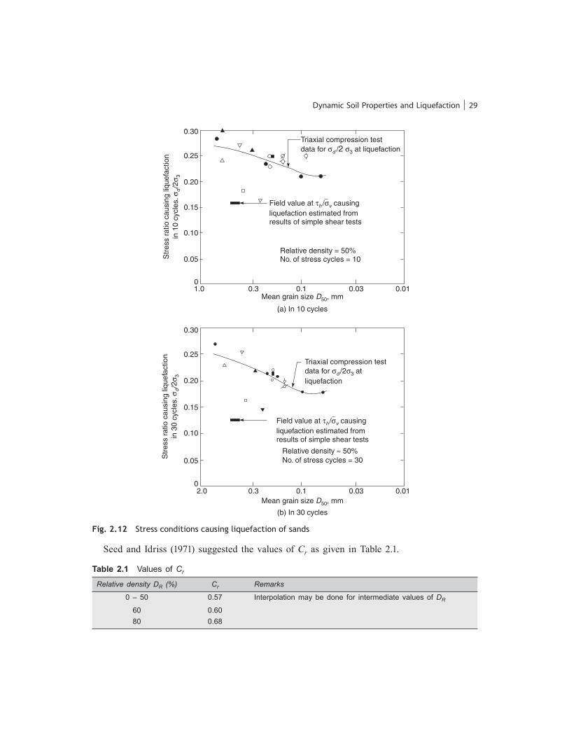
For evaluation of liquefaction potential, Seed and Idriss (1971) developed standard curves between cyclic resistance ratio (sd /2s3) versus mean grain size (D50) for 10 to 30 numbers of cycles of stress application for an initial relative density of compaction of 50% (Figs. 2.12 a and b). These curves were prepared by compiling the results of various tests conducted by several investigators on various types of sand. The values of cyclic resistance ratio (th/
__ s v) causing liquefaction, estimated from the results
of simple shear tests, have shown that the value of th/ __
s v is less than the corresponding value of sd/2s3 (Figs. 2.12 a and b). The two resistance ratio may be expressed by the following relation:
( th ___ sv ) field Dr
= ( sd ____ 2s3 )
triax 50 Cr
Dr ___ 50 ...(2.19)
where, DR = relative density (%), and Cr = correction factor.
Dynamic Soil Properties and Liquefaction 29
Seed and Idriss (1971) suggested the values of Cr as given in Table 2.1.
Table 2.1 Values of Cr
Relative density DR (%) Cr Remarks
0 – 50 0.57 Interpolation may be done for intermediate values of DR
60 0.60 80 0.68
Triaxial compression testdata for / at liquefactions sd 2 3
Field value at / causingliquefaction estimated fromresults of simple shear tests
t sh v
Relative density = 50%No. of stress cycles = 10
0.30
0.25
0.20
0.15
0.10
0.05Str
ess
ratio
cau
sing
liqu
efac
tion
in 1
0 cy
cles
./2
ss
d3
01.0 0.3 0.1 0.03 0.01
Mean grain size , mmD50
(a) In 10 cycles
0.30
0.25
0.20
0.15
0.10
0.05Str
ess
ratio
cau
sing
liqu
efac
tion
in 3
0 cy
cles
./2
ss
d3
2.0 0.3 0.1 0.03 0.010
Mean grain size , mmD50
(b) In 30 cycles
Field value at / causingliquefaction estimated fromresults of simple shear tests
t sh v
Relative density 50%No. of stress cycles = 30
ª
Triaxial compression testdata for /2 atliquefaction
s sd 3
Fig. 2.12 Stress conditions causing liquefaction of sands

30 Foundations and Retaining Structures
Sand compacted at a relative density more than 80% require very huge value of cyclic stress ratio for causing liquefaction. At a depth below the ground surface, liquefaction will occur if the shear stress induced by an earthquake is more than the shear resistance predicted by Eq. (2.19). By comparing the induced shear stresses and predicted shear resistances at various depths, liquefaction zone can be obtained. In a sand deposit consider a column of soil of height h and unit area of cross-section subjected to maximum ground acceleration amax (Fig. 2.13). Assuming the soil column to behave as a rigid body, the maximum shear stress tmax at a depth h is given by
tmax = ( gh __ g ) amax ...(2.20)
where, g = acceleration due to gravity, and g = unit weight of soil. Since the soil column behaves as a deformable body, the actual shear stress at depth h, (tmax)act is taken as
(tmax)act = rd . tmax = rd ( gh __ g ) amax ...(2.21)
where, rd = stress reduction factor. Seed and Idriss (1971) recommended the use of charts shown in Fig. 2.14 for obtaining the values of rd at various depths. In this figure the range of rd for different soil profiles alongwith the average value upto depth of 12 m is shown. The critical depth for development of liquefaction is usually less than 12 m.
Unit cross-sectionalareah
gh
amax
tmax = ( / g) .gh amax
Fig. 2.13 Maximum shear stress at a depth for a rigid soil column
0 0.2 0.4 0.6 0.8 1.0rd
0
6
12
18
24
30
Dep
th (
m)
Average value
Range ofdifferent soilprofiles
Fig. 2.14 Reduction factor rd versus depths (Seed and Idriss, 1971)
32 Foundations and Retaining Structures
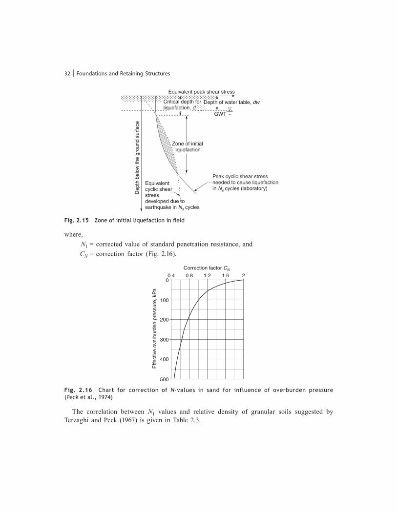
where, N1 = corrected value of standard penetration resistance, and CN = correction factor (Fig. 2.16).
Equivalent peak shear stress
Zone of initialliquefaction
GWT
Depth of water table, dw
Peak cyclic shear stressneeded to cause liquefactionin cycles (laboratory)Ns
Equivalentcyclic shearstressdeveloped due toearthquake in cyclesNs
Dep
th b
elow
the
grou
nd s
urfa
ce
Critical depth forliquefaction, d
Fig. 2.15 Zone of initial liquefaction in fi eld
Fig. 2.16 Chart for correction of N-values in sand for influence of overburden pressure (Peck et al., 1974)
0.4 0.8 1.2 1.6 20
100
200
300
400
500
Effe
ctiv
e ov
erbu
rden
pre
ssur
e, k
Pa
Correction factor CN
The correlation between N1 values and relative density of granular soils suggested by Terzaghi and Peck (1967) is given in Table 2.3.
Dynamic Soil Properties and Liquefaction 33
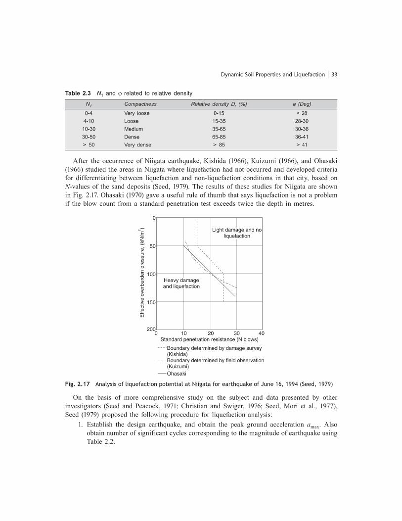
Table 2.3 N1 and j related to relative density
N1 Compactness Relative density Dr (%) j (Deg)
0-4 Very loose 0-15 < 28 4-10 Loose 15-35 28-30 10-30 Medium 35-65 30-36 30-50 Dense 65-85 36-41 > 50 Very dense > 85 > 41
After the occurrence of Niigata earthquake, Kishida (1966), Kuizumi (1966), and Ohasaki (1966) studied the areas in Niigata where liquefaction had not occurred and developed criteria for differentiating between liquefaction and non-liquefaction conditions in that city, based on N-values of the sand deposits (Seed, 1979). The results of these studies for Niigata are shown in Fig. 2.17. Ohasaki (1970) gave a useful rule of thumb that says liquefaction is not a problem if the blow count from a standard penetration test exceeds twice the depth in metres.
Light damage and noliquefaction
Heavy damageand liquefaction
Boundary determined by damage survey(Kishida)Boundary determined by field observation(Kuizumi)Ohasaki
0
50
100
150
2000 10 20 30 40
Effe
ctiv
e ov
erbu
rden
pre
ssur
e, (
kN/m
)2
Standard penetration resistance (N blows)
Fig. 2.17 Analysis of liquefaction potential at Niigata for earthquake of June 16, 1994 (Seed, 1979)
On the basis of more comprehensive study on the subject and data presented by other investigators (Seed and Peacock, 1971; Christian and Swiger, 1976; Seed, Mori et al., 1977), Seed (1979) proposed the following procedure for liquefaction analysis: 1. Establish the design earthquake, and obtain the peak ground acceleration amax. Also
obtain number of significant cycles corresponding to the magnitude of earthquake using Table 2.2.
34 Foundations and Retaining Structures
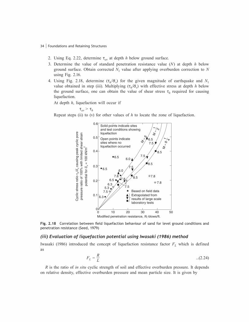
2. Using Eq. 2.22, determine tav at depth h below ground surface. 3. Determine the value of standard penetration resistance value (N) at depth h below
ground surface. Obtain corrected N1 value after applying overburden correction to N using Fig. 2.16.
4. Using Fig. 2.18, determine (th/ __
s v) for the given magnitude of earthquake and N1 value obtained in step (iii). Multiplying (th/
__ s v) with effective stress at depth h below
the ground surface, one can obtain the value of shear stress th required for causing liquefaction.
At depth h, liquefaction will occur if tav > th
Repeat steps (ii) to (v) for other values of h to locate the zone of liquefaction.
0.6
0 10 20 30 40 500
0.1
0.2
0.3
0.4
0.5
Extrapolated fromresults of large scalelaboratory tests
Based on field data
7.8
7.87.8
7.5
8.5
8.5
8.5
7.5
7.5
7.5
7.8
6.0
6.0
6.56.3
5.37.5
6.3
6.5
6.5
6.5
Solid points indicate sitesand test conditions showingliquefaction
Open points indicatesites where noliquefaction occurred
M6
ª
Mª
1 2
M8
ª1 4
Modified penetration resistance, -blows/ft.N1
Cyc
lic s
tres
s ra
tio/
caus
ing
peak
cyc
lic p
ore
pres
sure
rat
io o
f 100
% w
ith li
mite
d sh
ear
str a
inpo
tent
ial f
or=
100
kN
/m
ts
s
hv
v2
Fig. 2.18 Correlation between fi eld liquefaction behaviour of sand for level ground conditions and penetration resistance (Seed, 1979)
(iii) Evaluation of liquefaction potential using Iwasaki (1986) method
Iwasaki (1986) introduced the concept of liquefaction resistance factor FL which is defined as
FL = R __ L ...(2.24)
R is the ratio of in situ cyclic strength of soil and effective overburden pressure. It depends on relative density, effective overburden pressure and mean particle size. It is given by
Dynamic Soil Properties and Liquefaction 35
For 0.02 < D50 < 0.6 mm
R = 0.882 ÷ _______
N _______ __
s v + 70 + 0.225 log10 ( 0.35 ____ D50 ) ...(2.25)
For 0.6 < D50 < 2.0 mm
R = 0.882 ÷ _______
N _______ __
s v + 70 – 0.05 ...(2.26)
where, N = observed value of standard penetration resistance,
__ s v = effective overburden pressure at the depth under consideration for liquefaction
examination in kN/m2, D50 = mean grain size in mm, and L = ratio of dynamic load induced by seismic motion and effective overburden pressure. It is given by
L = amax ____ g
sv ___ __
s v rd ...(2.27)
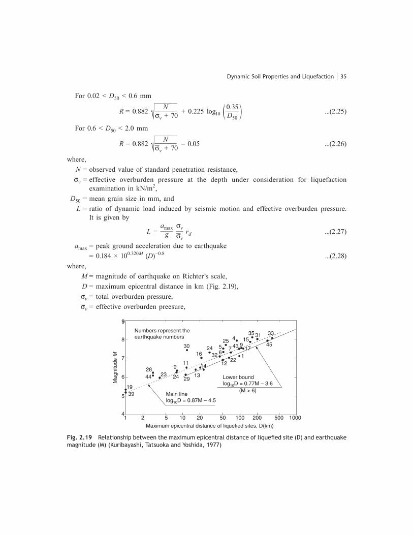
amax = peak ground acceleration due to earthquake = 0.184 × 100.320M (D)–0.8 ...(2.28)where, M = magnitude of earthquake on Richter’s scale, D = maximum epicentral distance in km (Fig. 2.19), sv = total overburden pressure,
__ s v = effective overburden preesure,
Fig. 2.19 Relationship between the maximum epicentral distance of liquefi ed site (D) and earthquake magnitude (M) (Kuribayashi, Tatsuoka and Yoshida, 1977)
9
3919
2844 23
9
24 2913
1411
1630 24
32 65
25 4
7 43 915
35 31 33
4517
122
12
Lower boundlog D = 0.77M – 3.610
Main linelog D = 0.87M – 4.510
(M > 6)
Numbers represent theearthquake numbers
1 2 5 10 20 50 100 200 500 1000
Maximum epicentral distance of liquefied sites, D(km)
9
8
7
6
5
4
Mag
nitu
deM

36 Foundations and Retaining Structures
rd = reduction factor to account the flexibility of the ground = 1 – 0.015 h, g = acceleration due to gravity, m/s2, and h = depth of plane below ground surface in m. For the soil not to liquefy FL should be greater than unity.
(iv) Evaluation of probability of initiation of liquefaction
Cetin et al. (2004) presented new correlations for obtaining probability of initiation of liquefaction at any depth ‘h’ below the ground surface. These new correlations eliminate several sources of bias intrinsic to previous, similar correlations, and provide greatly reduced overall uncertainty and variance. Key elements in the development of these new correlations are: (i) accumulation of a significantly expanded database of field performance case histories; (ii) use of improved knowledge and understanding of factors affecting interpretation of standard penetration test data; (iii) incorporation of improved understanding of factors affecting site-specific earthquake ground motions (including directivity effects, site-specific response, etc.); (iv) use of improved methods for assessment of in situ cyclic shear stress ratio; (v) screening of field data case histories on a quality/uncertainty basis; and (vi) use of high-order probabilistic tools (Bayesian updating). The resulting relationships not only provide greatly reduced uncertainty, they also help to resolve a number of corollary issues that have long been difficult and controversial including: (i) magnitude-correlated duration weighting factors, (ii) adjustments for fines content, and (iii) corrections for overburden stress. The procedure given by Cetin et al. (2004), for obtaining the probability of initiating liquefaction at any depth below the ground surface, can be summarized in the following steps:1. Obtain the value of standard penetration resistance (N) at the depth h below the ground surface. Correct it for overburden effect using Eq. (2.29)where, N1 = N CN ...(2.29) CN = (100/s¢v)
0.5 (Liao and Whiteman, 1986) ...(2.30) s¢v = effective overburden stress at depth h in kN/m2
If the value of CN works out more than 1.6 adopt CN = 1.6. The resulting N1 value is further corrected for energy, equipment and procedural effects to obtain fully standardized N1,60 value as:
N1,60 = N1. CR.CS.CB.CE ...(2.31)
where, CR = correction for short rod length, CS = correction for non-standardized sample configuration, CB = correction for borehole diameter, and CE = correction for hammer energy efficiency. CR may be obtained using Fig. 2.20.

38 Foundations and Retaining Structures
2. Obtain equivalent cyclic stress ratio (CSREq) using the following relation:
CSREq = 0.65 ( amax ____ g ) ( sv ___ s¢v
) rd ...(2.36)
where, amax = peak horizontal ground acceleration, g = acceleration due to gravity, sv = total vertical stress at depth h, s¢v = effective vertical stress at depth h, and rd = non-linear shear mass participation factor (Fig. 2.21) (Mayfield et al., 2010).
0.20.2 0.4 0.6 0.8 1.00
5
10
15
20
Dep
th,
(m)
z
Mean
Mean +/– s
Depth reduction factor, rd
(Standard deviation)
Fig. 2.21 Computed mean rd profi les with vs,12 = 175 m/ s for 475-year and 2,475-year peak acceleration and mean magnitude for Butte, Mont.; Charleston, S.C., Eureka, Calif.; Memphis, Tenn.; Portland, Ore.; Salt Lake City; San Francisco; San Jose, Calif.; Santa Monica, Calif.; and Seattle (after Cetin, 2004).
3. Obtain CSREq, M = 7.5 which represents the equivalent CSREq for a duration typical of an average equal of magnitude of earthquake (Mw) equal to 7.5, using the following relation:
CSREq, M = 7.5 = CSREq
______ DWFM ...(2.37)
where, DWFM is duration weighting factor and is obtained using Fig. 2.22.4. Convert the value of CSREq, M = 7.5 corrosponding to 1 atmosphere pressure using the following relation:
CSREq, M = 7.5, 1 at = CSREq, M = 7.5
___________ Ks = CSR*
Eq ...(2.38)
where, Ks = (s¢v)
f – 1 ...(2.39) s¢v = Effective overburden stress in kg/cm2.

40 Foundations and Retaining Structures
ILLUSTRATIVE EXAMPLES
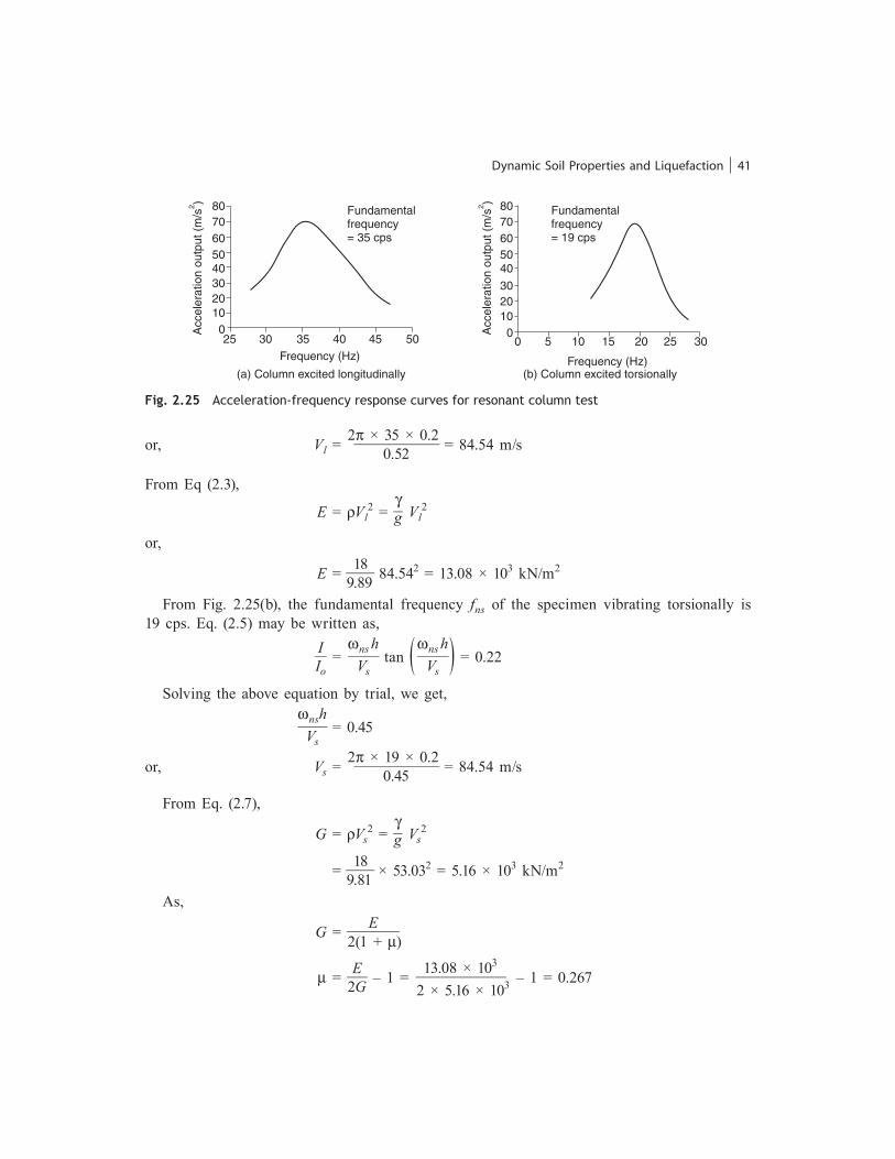
Example 2.1 A 200 mm high specimen of clayey sand with a unit weight of 18.0 kN/m3 is tested in a resonant column device having weight of specimen to weight of loading system ratio as 0.3 and ratio of mass polar moment of inertia of the specimen to mass polar moment of inertia torsional loading system as 0.22. When the column is excited longitudinally, the frequency-response curve as shown in Fig. 2.25(a) was obtained. Figure 2.25(b) shows the frequency-response curve when the column was excited torsionally. Determine the Young’s modulus, shear modulus and Poisson’s ratio of the soil.Solution From Fig. 2.25(a), the fundamental frequency fnl of the specimen vibrating longitudinally is 35 cps. The Eq. (2.1) may be written as,
W ___ Wo =
wnl h ____ Vl tan ( wnl h ____ Vl
) = 0.3
Solving the above equation by trial, we get,
wnl h ____ Vl
= 0.52
0.6
0.5
0.4
0.3
0.2
0.1
0.00 10 20 30 40
Pro-1985 data“Now” data
CS
R*
eq
N1,60,CS
M=
7.5
= 1
.0 a
tmW
s v
80% 20%95% 5%50%
Liqu
efie
d
Mar
gina
l
Non
-liq
uefie
d
PL
Fig. 2.24 Recommended probabilistic standard penetration test-based liquefaction triggering correla-tion for Mw = 7.5 and sv = 1.0 atm (after Cetin, 2004).
Dynamic Soil Properties and Liquefaction 41
or, Vl = 2p × 35 × 0.2 ____________ 0.52 = 84.54 m/s
From Eq (2.3),
E = rVl2 =
g __ g Vl
2
or,
E = 18 ____ 9.89 84.542 = 13.08 × 10³ kN/m2
From Fig. 2.25(b), the fundamental frequency fns of the specimen vibrating torsionally is 19 cps. Eq. (2.5) may be written as,
I __ Io =
wns h _____ Vs tan ( wns h _____ Vs
) = 0.22
Solving the above equation by trial, we get,
wnsh ____ Vs
= 0.45
or, Vs = 2p × 19 × 0.2 ____________ 0.45 = 84.54 m/s
From Eq. (2.7),
G = rVs2 =
g __ g Vs
2
= 18 ____ 9.81 × 53.032 = 5.16 × 10³ kN/m2
As,
G = E _______ 2(1 + m)
m = E ___ 2G – 1 = 13.08 × 10³ ____________
2 × 5.16 × 103 – 1 = 0.267
Fig. 2.25 Acceleration-frequency response curves for resonant column test
Fundamentalfrequency= 19 cps
0 5 10 15 20 25 30
Frequency (Hz)
8070605040
3020100
80706050403020100
Fundamentalfrequency= 35 cps
25 30 35 40 45 50
Frequency (Hz)
(a) Column excited longitudinally (b) Column excited torsionally
Acc
eler
atio
n ou
tput
(m
/s)2
Acc
eler
atio
n ou
tput
(m
/s)2
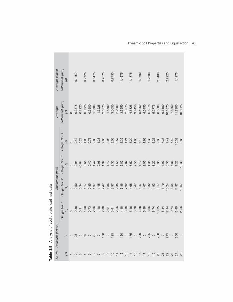
Dynamic Soil Properties and Liquefaction 43
Tabl
e 2.
5 A
naly
sis
of c
yclic
pla
te lo
ad t
est
data
Sr.
No.
P
ress
ure
(kN
/m2 )
Set
tlem
ent
(mm
) Av
erag
e Av
erag
e el
astic
G
auge
No.
1
Gau
ge N
o. 2
G
auge
No.
3
Gau
ge N
o. 4
se
ttlem
ent
(mm
) se
ttlem
ent
(mm
)
(1)
(2)
(3)
(4)
(5)
(6)
(7)
(8)
1.
0
0 0
0 0
0
2.
25
0.38
0.
50
0.04
0.
43
0.33
75
0.11
50
3.
0 0.
31
0.34
–0
.04
0.28
0.
2225
4.
50
1.00
1.
17
0.65
1.
03
0.96
25
0.27
25
5.
0 0.
73
0.85
0.
40
0.78
0.
6900
6.
75
2.06
1.
97
1.42
2.
03
1.87
00
0.54
75
7.
0 1.
48
1.45
0.
98
1.38
1.
3225
8.
100
2.86
2.
47
1.92
2.
90
2.53
75
0.70
75
9.
0 2.
01
1.86
1.
42
2.03
1.
8300
10.
125
3.41
2.
97
2.30
3.
58
3.06
50
0.77
50
11.
0 2.
56
2.35
1.
68
2.57
2.
2900
12.
150
4.18
3.
86
2.82
4.
32
3.79
50
1.46
75
13.
0 3.
16
2.92
2.
02
1.21
2.
3275
14.
175
5.16
4.
65
3.52
5.
20
4.63
25
1.18
75
15.
0 3.
76
3.47
2.
55
4.00
3.
4450
16.
200
6.28
5.
47
4.10
6.
13
5.49
50
1.15
00
17.
0 5.
38
4.07
2.
95
4.98
4.
3450
18.
225
8.06
6.
32
4.35
7.
38
6.52
75
1.25
00
19.
0 6.
74
4.92
3.
22
6.23
5.
2775
20.
250
10.3
5 8.
17
6.35
9.
33
8.55
00
2.04
00
21.
0 8.
84
5.79
4.
03
7.38
6.
5100
22.
275
12.1
4 10
.24
8.56
9.
49
10.1
075
2.22
25
23.
0 9.
74
8.54
5.
86
7.40
7.
8850
24.
300
13.4
5 11
.87
11.2
2 10
.38
11.7
300
1.12
75
25.
0 11
.56
10.6
7 10
.30
9.88
10
.602
5
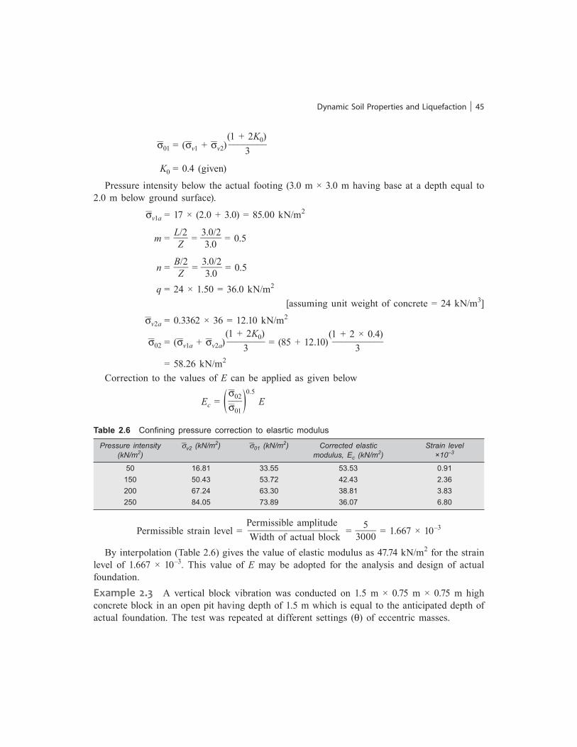
Dynamic Soil Properties and Liquefaction 45
__
s 01 = ( __
s v1 + __
s v2) (1 + 2K0) ________ 3
K0 = 0.4 (given)
Pressure intensity below the actual footing (3.0 m × 3.0 m having base at a depth equal to 2.0 m below ground surface).
__
s v1a = 17 × (2.0 + 3.0) = 85.00 kN/m2
m = L/2 ___ Z = 3.0/2 _____ 3.0 = 0.5
n = B/2 ___ Z = 3.0/2 _____ 3.0 = 0.5
q = 24 × 1.50 = 36.0 kN/m2
[assuming unit weight of concrete = 24 kN/m3]
__
s v2a = 0.3362 × 36 = 12.10 kN/m2
__
s 02 = ( __
s v1a + __
s v2a) (1 + 2K0) ________ 3 = (85 + 12.10)
(1 + 2 × 0.4) ___________ 3
= 58.26 kN/m2
Correction to the values of E can be applied as given below
Ec = ( __
s 02 ___ __
s 01 ) 0.5
E
Table 2.6 Confining pressure correction to elasrtic modulus
Pressure intensity __
s v2 (kN/m2) __
s 01 (kN/m2) Corrected elastic Strain level (kN/m2) modulus, Ec (kN/m2) ×10–3
50 16.81 33.55 53.53 0.91 150 50.43 53.72 42.43 2.36 200 67.24 63.30 38.81 3.83 250 84.05 73.89 36.07 6.80
Permissible strain level = Permissible amplitude
___________________ Width of actual block = 5 _____ 3000 = 1.667 × 10⁻³
By interpolation (Table 2.6) gives the value of elastic modulus as 47.74 kN/m2 for the strain level of 1.667 × 10⁻³. This value of E may be adopted for the analysis and design of actual foundation.Example 2.3 A vertical block vibration was conducted on 1.5 m × 0.75 m × 0.75 m high concrete block in an open pit having depth of 1.5 m which is equal to the anticipated depth of actual foundation. The test was repeated at different settings (q) of eccentric masses.

Dynamic Soil Properties and Liquefaction 47
where,
__ s v =
__ s v1 +
__ s v2,
__
s v1 = effective overburden pressure at the depth under consideration, and
__ s v2 = increase in vertical pressure due to weight of block.
Assuming that top 2.0 m soil has a moist unit weight of 18 kN/m3 and saturated unit weight below water table is 20 kN/m3, then
__
s v1 = 18 × 2.0 + 10 × 0.25 ____ 2 = 37.25 kN/m2
From Taylor (1948):
__
s v2 = 4q
___ 4p [ 2mn ÷ __________
m2 + n2 + 1 ________________ m2 + n2 + 1 + m2n2 m
2 + n2 + 2 __________ m2 + n2 + 1
+ sin–1 2mn ÷
__________ m2 + n2 + 1 ________________
m2 + n2 + 1 + m2n2 ] m = L/2 ___ Z = 1.5/2 _____ 0.75 = 1.0
n = L/2 ___ Z = 0.75/2 ______ 0.75 = 0.5
q = 24 × 0.75 = 18.0 kN/m2
[assuming unit weight of concrete = 24 kN/m3] Substituting the above values of m, n, and q in the expression of
__ s v2, we get
__
s v2 = 0.4808q = 8.65 kN/m2
__
s v = 37.25 + 8.65 = 45.90 kN/m2
k0 = 1 – sin f = 1 – sin 30° = 0.5
__
s 01 = 45.90 (1 + 2 × 0.5)
___________ 3 = 30.60 kN/m2
For the actual foundation
__ s v1 = 18 × 2.0 + 10 × 2.5 = 61.0 kN/m2
m = 4.0/2 _____ 3.0 = 0.67
n = 3.0/2 _____ 3.0 = 0.50
q = 24 × 1.0 = 24.0 kN/m2
[assuming unit weight of concrete = 24 kN/m3] Substituting the above values of m, n, and q in the expression of
__ s v2, we get
__
s v2 = 0.4035q = 9.68 kN/m2
__
s v = 61.0 + 9.68 = 70.68 kN/m2
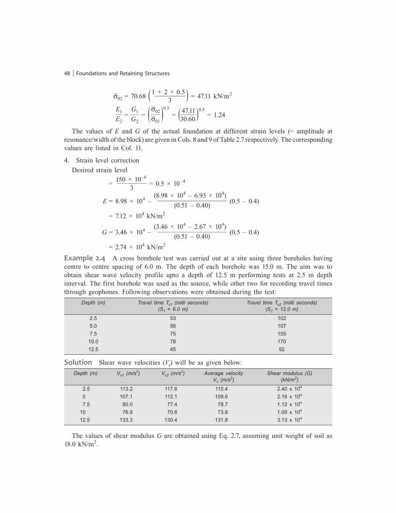
48 Foundations and Retaining Structures
__
s 02 = 70.68 ( 1 + 2 × 0.5 _________ 3 ) = 47.11 kN/m2
E1 ___ E2
= G1 ___ G2
= ( __
s 02 ___ __
s 01 ) 0.5
= ( 47.11 _____ 30.60 ) 0.5 = 1.24
The values of E and G of the actual foundation at different strain levels (= amplitude at resonance/width of the block) are given in Cols. 8 and 9 of Table 2.7 respectively. The corresponding values are listed in Col. 11.
4. Strain level correction Desired strain level
= 150 × 10–6 _________ 3 = 0.5 × 10⁻⁴
E = 8.98 × 10⁴ – (8.98 × 10⁴ – 6.93 × 10⁴)
_____________________ (0.51 – 0.40) (0.5 – 0.4)
= 7.12 × 10⁴ kN/m2
G = 3.46 × 10⁴ – (3.46 × 10⁴ – 2.67 × 10⁴)
_____________________ (0.51 – 0.40) (0.5 – 0.4)
= 2.74 × 10⁴ kN/m2
Example 2.4 A cross borehole test was carried out at a site using three boreholes having centre to centre spacing of 6.0 m. The depth of each borehole was 15.0 m. The aim was to obtain shear wave velocity profile upto a depth of 12.5 m performing tests at 2.5 m depth interval. The first borehole was used as the source, while other two for recording travel times through geophones. Following observations were obtained during the test: Depth (m) Travel time Ts1 (milli seconds) Travel time Ts2 (milli seconds) (S1 = 6.0 m) (S2 = 12.0 m)
2.5 53 102 5.0 56 107 7.5 75 155 10.0 78 170 12.5 45 92
Solution Shear wave velocities (Vs) will be as given below: Depth (m) Vs1 (m/s2) Vs2 (m/s2) Average velocity Shear modulus (G) Vs (m/s2) (kN/m2)
2.5 113.2 117.6 115.4 2.40 x 10⁴
5 107.1 112.1 109.6 2.16 x 10⁴
7.5 80.0 77.4 78.7 1.12 x 10⁴
10 76.9 70.6 73.8 1.00 x 10⁴
12.5 133.3 130.4 131.8 3.13 x 10⁴
The values of shear modulus G are obtained using Eq. 2.7, assuming unit weight of soil as 18.0 kN/m2.
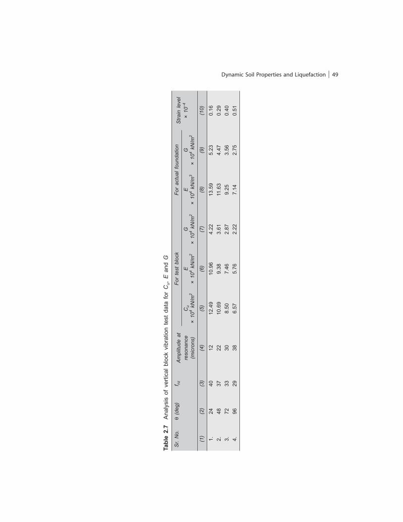
Dynamic Soil Properties and Liquefaction 49
Tabl
e 2.
7 A
naly
sis
of v
ertic
al b
lock
vib
ratio
n te
st d
ata
for
Cu,
E a
nd G
Sr.
No.
q
(deg
) f n
z A
mpl
itude
at
Fo
r te
st b
lock
For
actu
al f
ound
atio
n S
train
leve
l
re
sona
nce
Cu
E
G
E
G
× 10
–4
(mic
rons
) ×
104 k
N/m
2 ×
104 k
N/m
2 ×
104 k
N/m
2 ×
104 k
N/m
3 ×
104 k
N/m
2
(1
) (2
) (3
) (4
) (5
) (6
) (7
) (8
) (9
) (1
0)
1.
24
40
12
12
.49
10.9
6 4.
22
13.5
9 5.
23
0.16
2.
48
37
22
10
.69
9.38
3.
61
11.6
3 4.
47
0.29
3.
72
33
30
8.
50
7.46
2.
87
9.25
3.
56
0.40
4.
96
29
38
6.
57
5.76
2.
22
7.14
2.
75
0.51
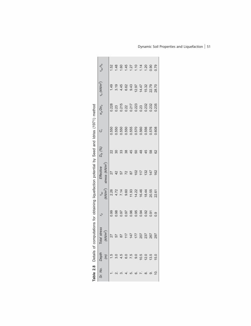
Dynamic Soil Properties and Liquefaction 51
Tabl
e 2.
8 D
etai
ls o
f co
mpu
tatio
ns f
or o
btai
ning
liqu
efac
tion
pote
ntia
l by
See
d an
d Id
riss
(197
1) m
etho
d
Sr.
No.
D
epth
To
tal s
tress
r d
t a
v E
ffect
ive
DR (
%)
Cr
s d /2
s 3
t h (k
N/m
2 ) t a
v /t h
(m)
(kN
/m2 )
(k
N/m
2 ) st
ress
(kN
/m2 )
1.
1.
5 27
0.
99
2.26
27
22
0.
550
0.22
8 1.
49
1.52
2.
3.
0 57
0.
98
4.72
42
30
0.
550
0.23
3.
19
1.48
3.
4.
5 87
0.
97
7.14
57
33
0.
550
0.21
5 4.
45
1.60
4.
6.
0 11
7 0.
97
9.60
72
38
0.
550
0.22
6.
62
1.45
5.
7.
5 14
7 0.
96
11.9
3 87
45
0.
555
0.21
7 9.
43
1.27
6.
9.
0 17
7 0.
95
14.2
2 10
2 50
0.
570
0.22
3 12
.97
1.10
7.
10
.5
207
0.94
16
.46
117
48
0.56
0 0.
23
14.4
7 1.
14
8.
12.0
23
7 0.
92
18.4
4 13
2 45
0.
556
0.23
2 15
.32
1.20
9.
13
.5
267
0.91
20
.55
147
58
0.57
6 0.
232
22.7
9 0.
90
10.
15.0
29
7 0.
9 22
.61
162
62
0.60
8 0.
235
28.7
0 0.
79
52 Foundations and Retaining Structures
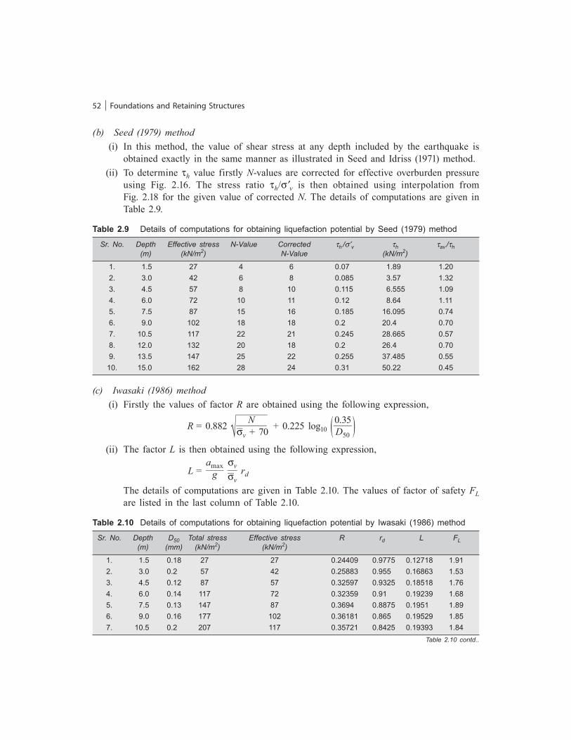
(b) Seed (1979) method (i) In this method, the value of shear stress at any depth included by the earthquake is
obtained exactly in the same manner as illustrated in Seed and Idriss (1971) method. (ii) To determine th value firstly N-values are corrected for effective overburden pressure
using Fig. 2.16. The stress ratio th/s¢v is then obtained using interpolation from Fig. 2.18 for the given value of corrected N. The details of computations are given in Table 2.9.
Table 2.9 Details of computations for obtaining liquefaction potential by Seed (1979) method
Sr. No. Depth Effective stress N-Value Corrected th /s¢v th tav /th (m) (kN/m2) N-Value (kN/m2)
1. 1.5 27 4 6 0.07 1.89 1.20 2. 3.0 42 6 8 0.085 3.57 1.32 3. 4.5 57 8 10 0.115 6.555 1.09 4. 6.0 72 10 11 0.12 8.64 1.11 5. 7.5 87 15 16 0.185 16.095 0.74 6. 9.0 102 18 18 0.2 20.4 0.70 7. 10.5 117 22 21 0.245 28.665 0.57 8. 12.0 132 20 18 0.2 26.4 0.70 9. 13.5 147 25 22 0.255 37.485 0.55 10. 15.0 162 28 24 0.31 50.22 0.45
(c) Iwasaki (1986) method (i) Firstly the values of factor R are obtained using the following expression,
R = 0.882 ÷ _______
N _______ __
s v + 70 + 0.225 log10 ( 0.35 ____ D50 )
(ii) The factor L is then obtained using the following expression,
L = amax ____ g
sv ___ __
s v rd
The details of computations are given in Table 2.10. The values of factor of safety FL are listed in the last column of Table 2.10.
Table 2.10 Details of computations for obtaining liquefaction potential by Iwasaki (1986) method
Sr. No. Depth D50 Total stress Effective stress R rd L FL (m) (mm) (kN/m2) (kN/m2)
1. 1.5 0.18 27 27 0.24409 0.9775 0.12718 1.91 2. 3.0 0.2 57 42 0.25883 0.955 0.16863 1.53 3. 4.5 0.12 87 57 0.32597 0.9325 0.18518 1.76 4. 6.0 0.14 117 72 0.32359 0.91 0.19239 1.68 5. 7.5 0.13 147 87 0.3694 0.8875 0.1951 1.89 6. 9.0 0.16 177 102 0.36181 0.865 0.19529 1.85 7. 10.5 0.2 207 117 0.35721 0.8425 0.19393 1.84
Table 2.10 contd..
54 Foundations and Retaining Structures
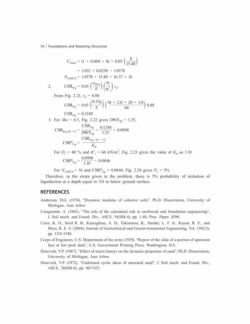
Cfines = (1 + 0.004 × 8) + 0.05 ( 8 _____ 15.48 ) = 1.032 + 0.0258 = 1.0578 N1,60CS = 1.0578 × 15.48 = 16.37 ª 16
2. CSREq = 0.65 ( amax ____ g ) ( sv ___ s¢v
) rd
From Fig. 2.21, rd = 0.88
CSREq = 0.65 ( 0.15g _____ g ) ( 18 × 2.0 + 20 × 3.0 ________________ 66 ) 0.88
CSREq = 0.1248 3. For Mw = 6.5, Fig. 2.22 gives DWFM = 1.25,
CSREq,M = 7.5 = CSREq
______ DWFM = 0.1248 ______ 1.25 = 0.0998
CSR*Eq = CSREq, M = 7.5
___________ Ks
For Dr = 40 % and s¢v = 66 kN/m2, Fig. 2.23 gives the value of Ks as 1.18
CSR*Eq = 0.0998 ______ 1.18 = 0.0846
For N1,60CS = 16 and CSR*Eq = 0.0846, Fig. 2.24 gives PL = 5% Therefore, in the strata given in the problem, there is 5% probability of initiation of liquefaction at a depth equal to 5.0 m below ground surface.
REFERENCES
Anderson, D.G. (1974), “Dynamic modulus of cohesive soils”, Ph.D. Dissertation, University of Michigan, Ann Arbor.
Casagrande, A. (1965), “The role of the calculated risk in earthwork and foundation engineering”, J. Soil mech. and Found. Div., ASCE, 91(SM-4), pp. 1-40, Proc. Paper. 4390.
Cetin, K. O., Seed R. B., Kiureghian, A. D., Tokimatsu, K., Harder, L. F. Jr., Kayen, R. E., and Moss, R. E. S. (2004), Journal of Geotechnical and Geoenvironmental Engineering, Vol. 130(12), pp. 1314-1340.
Corps of Engineers, U.S. Department of the army (1939), “Report of the slide of a portion of upstream face at fort peck dam”, U.S. Government Printing Press, Washington, D.S.
Drnevich, V.P. (1967), “Effect of strain history on the dynamic properties of sand”, Ph.D. Dissertation, University of Michigan, Ann Arbor.
Drnevich, V.P. (1972), “Undrained cyclic shear of saturated sand”, J. Soil mech. and Found. Div., ASCE, 38(SM-8), pp. 807-825.
56 Foundations and Retaining Structures
Seed, H. B. (1979)’ “Soil liquefaction and cyclic mobility for level ground during earthquakes”, J. Geotech Eng. Div., ASCE, 10(GT-2), pp. 201-255.
Teraghi, K. L., and Peck, R. B. (1967), “Soil mechanics in engineering practice”, John Wiley and Sons Inc., New York.
Waterways Experiments Station, U. S. Corps of Engineers (1967), “Potamology investigation, report 12-18, verification of empirical method for determining river bank stability”, 1965 Data, Vicksburg, Mississippi.
Woods, R.D. (1978), “Measurement of dynamic soil properties: state-of-the-art”, Proc. ASCE Spec. conf. Earthquake Eng. Soil Dyn., Pasadena, CA, Vol. 1, pp. 91-180.
Youd, T. L., et al. (2001). “Liquefaction resistance of soils; summary report from the 1996 NCEER and 1998 NCEER/NSF workshops on evaluation of liquefaction resistance of soils.” J. Geotech. Geoenviron. Eng., 127(10), 817–833.
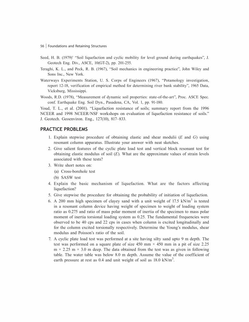
PRACTICE PROBLEMS
1. Explain stepwise procedure of obtaining elastic and shear modulii (E and G) using resonant column apparatus. Illustrate your answer with neat sketches.
2. Give salient features of the cyclic plate load test and vertical block resonant test for obtaining elastic modulus of soil (E). What are the approximate values of strain levels associated with these tests?
3. Write short notes on: (a) Cross-borehole test (b) SASW test 4. Explain the basic mechanism of liquefaction. What are the factors affecting
liquefaction? 5. Give stepwise the procedure for obtaining the probability of initiation of liquefaction. 6. A 200 mm high specimen of clayey sand with a unit weight of 17.5 kN/m3 is tested
in a resonant column device having weight of specimen to weight of loading system ratio as 0.275 and ratio of mass polar moment of inertia of the specimen to mass polar moment of inertia torsional loading system as 0.25. The fundamental frequencies were observed to be 40 cps and 22 cps in cases when column is excited longitudinally and for the column excited torsionally respectively. Determine the Young’s modulus, shear modulus and Poisson’s ratio of the soil.
7. A cyclic plate load test was performed at a site having silty sand upto 9 m depth. The test was performed on a square plate of size 450 mm × 450 mm in a pit of size 2.25 m × 2.25 m × 3.0 m deep. The data obtained from the test was as given in following table. The water table was below 8.0 m depth. Assume the value of the coefficient of earth pressure at rest as 0.4 and unit weight of soil as 18.0 kN/m3.
58 Foundations and Retaining Structures
adopted for the design of actual foundation. Limiting vertical amplitude of machine is 100 microns. Assume Poisson’s ratio as 0.3.
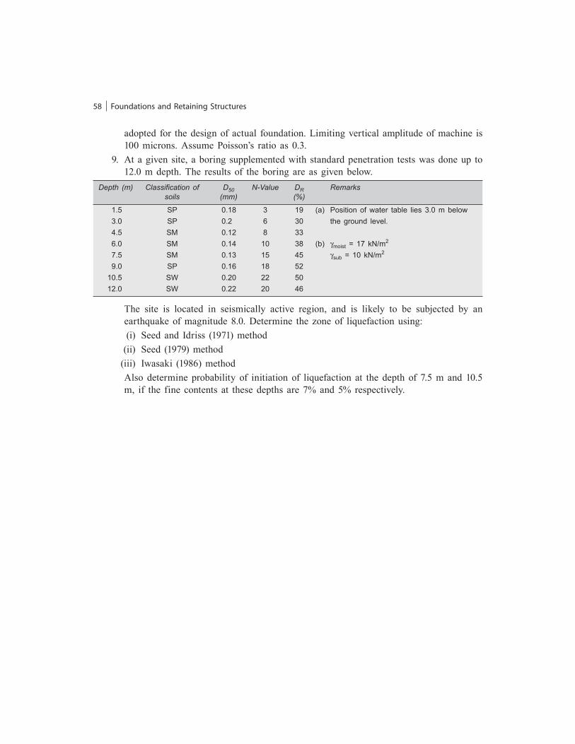
9. At a given site, a boring supplemented with standard penetration tests was done up to 12.0 m depth. The results of the boring are as given below.
Depth (m) Classification of D50 N-Value DR Remarks soils (mm) (%)
1.5 SP 0.18 3 19 (a) Position of water table lies 3.0 m below 3.0 SP 0.2 6 30 the ground level. 4.5 SM 0.12 8 33 6.0 SM 0.14 10 38 (b) gmoist = 17 kN/m2
7.5 SM 0.13 15 45 gsub = 10 kN/m2
9.0 SP 0.16 18 52 10.5 SW 0.20 22 50 12.0 SW 0.22 20 46
The site is located in seismically active region, and is likely to be subjected by an earthquake of magnitude 8.0. Determine the zone of liquefaction using:
(i) Seed and Idriss (1971) method (ii) Seed (1979) method (iii) Iwasaki (1986) method Also determine probability of initiation of liquefaction at the depth of 7.5 m and 10.5
m, if the fine contents at these depths are 7% and 5% respectively.