dynamic response and permanent displacement …
TRANSCRIPT

DYNAMIC RESPONSE AND PERMANENT DISPLACEMENT
ANALYSIS OF AKKÖPRÜ DAM
A THESIS SUBMITTED TO
THE GRADUATE SCHOOL OF NATURAL AND APPLIED SCIENCES
OF
THE MIDDLE EAST TECHNICAL UNIVERSITY
BY
DEN�Z ÜLGEN
IN PARTIAL FULLFILLMENT OF THE REQUIREMENTS FOR THE
DEGREE OF
MASTER OF SCIENCE
IN
THE DEPARTMENT OF CIVIL ENGINEERING
JANUARY 2004

Approval of the Graduate School of Natural and Applied Sciences.
Prof. Dr. Canan ÖZGEN Director I certify that this thesis satisfies all the requirements as a thesis for the degree of Master of Science.
Prof. Dr. Erdal ÇOKÇA Head of Department
This is to certify that we have read this thesis and that in our opinion it is fully adequate, in scope and quality, as a thesis for the degree of Master of Science.
Prof. Dr. M. Yener ÖZKAN Supervisor
Examining Committee Members
Prof. Dr. Altay B�RAND
Prof. Dr. M. Yener ÖZKAN
Prof. Dr. Orhan EROL
Asst. Prof. Dr. K. Önder ÇET�N
Gülru S. YILDIZ (M.S.)

iii
ABSTRACT
DYNAMIC RESPONSE AND PERMANENT DISPLACEMENT
ANALYSIS OF AKKÖPRÜ DAM
ÜLGEN, Deniz
M.S., Department of Civil Engineering
Supervisor: Prof. Dr. M. Yener ÖZKAN
January 2004, 115 pages
In this study, dynamic response of Akköprü Dam under earthquake motions
is analyzed and the permanent displacements are evaluated. Initially, the critical slip
surface of the dam and the corresponding yield acceleration are determined by using
the computer program SLOPE. Then, by employing the finite element program
SAP2000, static analyses are performed to obtain the mean effective stresses which
are used in the determination of dynamic material properties of the dam. Four
different scenario earthquakes having a magnitude of 7 are used in the dynamic
analyses. Two of those scenarios are taken from European Strong Motion Database
and the others are generated by XS artificial earthquake generation program prepared
by Erdik (1992). Dynamic analyses of the dam are carried out by the finite element
program TELDYN. Permanent displacements of the critical slip surface are
calculated by utilizing the Newmark method. Consequently, for an earthquake
having a magnitude of M=7 and a peak ground acceleration of 0.20g, the maximum
permanent displacement of the dam is found to be 15.90 cm. Furthermore, the
permanent displacements of the dam are calculated under base motions having
different peak ground acceleration values and it is observed that the rate of increase

iv
in the amount of permanent displacements is greater than the increase in the amount
of peak ground accelerations.
Keywords: Embankment Dams, Rockfill Dams, Dam Safety, Earthquakes, Soil
Dynamics, Dynamic Analysis, Finite Element Method, Permanent
Displacement

v
ÖZ
AKKÖPRÜ BARAJININ DEPREM TEPK�LER� VE KALICI
DEFORMASYON ANAL�Z�
ÜLGEN, Deniz
Yüksek Lisans, �n�aat Mühendisli�i Bölümü
Tez Yöneticisi: Prof. Dr. M. Yener ÖZKAN
Ocak 2004, 115 sayfa
Bu çalı�mada, Akköprü Barajının deprem hareketleri altındaki dinamik
tepkilerinin analizi yapılmı� ve kalıcı deformasyonları de�erlendirilmi�tir. �lk olarak,
kritik kayma yüzeyi ve ona kar�ılık gelen kayma ivmesi bilgisayar programı SLOPE
kullanılarak bulunmu�tur. Bundan sonra, barajın dinamik malzeme özelliklerininin
belirlenmesinde gerekli olan ortalama efektif gerilmelerini bulmak için sonlu
elemanlar propramı SAP2000 ile statik analiz yapılmı�tır. Dinamik analizlerde 7
büyüklü�ünde farklı dört senaryo deprem kullanılmı�tır. Senaryo depremlerden ikisi
Avrupa Kuvvetli Yer Hareketleri Veritabanından alınmı� ve di�erleri de Erdik(1992)
tarafından hazırlanan yapay deprem hareketi üreten XS programı ile olu�turulmu�tur.
Barajın dinamik analizleri sonlu elemanlar programı TELDYN kullanılarak
yapılmı�tır. Kritik kayma yüzeyindeki kalıcı deformasyonlar Newmark metodundan
yararlanılarak hesaplanmı�tır. Sonuç olarak 0.20g maksimum yer ivmesine sahip 7
büyüklü�ündeki bir deprem için barajın maksimum kalıcı deformasyonu 15.90 cm
olarak bulunmu�tur. Bununla beraber, farklı maksimum yer ivme de�erlerine sahip
deprem hareketleri altında barajın kalıcı deformasyonları hesaplanmı� ve kalıcı

vi
deformasyon miktarındaki artı� oranının ivme miktarındaki artı� oranından fazla
oldu�u gözlenmi�tir.
Anahtar Kelimeler: Dolgu Barajlar, Kaya Dolgu Barajlar, Baraj Emniyeti,
Depremler, Zemin Dinami�i, Dinamik Analiz, Sonlu Elemanlar
Metodu, Kalıcı Deformasyon

vii
Dedicated to MY FAMILY

viii
ACKNOWLEDGEMENTS
I would like to express my gratitude to my thesis supervisor Prof. Dr. M.
Yener ÖZKAN for his wise guidance in preparation of this thesis and teaching me
soil dynamics. I would also like to thank him for his general help and friendly
supports.
Dr. Ramazan DEM�RTA�, Vehbi B�LG� and Mehmet ÖZYAZICIO�LU
are also deeply acknowledged for their valuable supports and comments throughout
the study.
I would also like to thank to Asst. Prof. Dr. K. Önder ÇET�N for his help
and teaching me geotechnical earthquake engineering.
Also, I would like to thank to Burçin TUNA and Hasan MERCAN for their
help in computer related works, especially in Matlab and programming languages.
Finally, I would like to thank to my dear family for their continuous support
and friendship throughout the study.

ix
TABLE OF CONTENTS
ABSTRACT .......................................................................................................... iii
ÖZ............................................................................................................................v
ACKNOWLEDGEMENTS................................................................................ viii
TABLE OF CONTENTS...................................................................................... ix
LIST OF TABLES............................................................................................... xii
LIST OF FIGURES .............................................................................................xiv
LIST OF SYMBOLS ......................................................................................... xvii
CHAPTER I............................................................................................................1
1. INTRODUCTION...........................................................................................1
1.1 General ......................................................................................................1
1.2 Aim of the Study........................................................................................4
CHAPTER II ..........................................................................................................5
2. STATIC AND DYNAMIC ANALYSES OF EMBANKMENT DAMS........5
2.1 Static Analysis of Embankment Dams......................................................5
2.2 Design Ground Motion..............................................................................6
2.2.1 Estimation of Peak Ground Acceleration ..........................................8
2.2.2 Estimation of the Predominant Period ............................................10
2.2.3 Estimation of Duration .....................................................................10
2.3 Dynamic Analysis of Embankment Dams ..............................................12
2.3.1 Pseudostatic Method of Analysis......................................................12
2.3.2 Shear Beam Method .........................................................................15
2.3.3 Finite element method ......................................................................18

x
2.4 Equivalent Linear Model ........................................................................19
2.5 Permanent Displacement Analysis..........................................................25
CHAPTER III.......................................................................................................31
3. AKKÖPRÜ DAM AND SEISMICITY OF THE SITE ..............................31
3.1 General Information About Dalaman - Akköprü Dam .........................31
3.1.1 Characteristics of the Project...........................................................31
3.1.2 Geology and the Foundation ............................................................34
3.1.3 The Dam Embankment ....................................................................35
3.2 Seismicity of Akköprü Dam Site .............................................................38
3.3 Design Earthquake Ground Motion .......................................................39
3.3.1 Probabilistic Assessment ..................................................................39
3.3.2 Deterministic Assessment .................................................................45
3.3.2.1 Acceleration – Attenuation Approach.......................................45
3.4 Design Peak Ground Acceleration..........................................................46
3.5 Estimating Input Ground Motion...........................................................46
CHAPTER IV .......................................................................................................50
4. ANALYSES OF AKKÖPRÜ DAM..............................................................50
4.1 Analyses Procedure for Akköprü Dam ..................................................50
4.2 Pseudo-Static Analyses of Akköprü Dam...............................................51
4.3 Static Analyses of Akköprü Dam............................................................52
4.4 Dynamic Material Properties of Akköprü Dam.....................................59
4.5 Determination of Input Ground Motions to be Used in the Dynamic
Analysis..........................................................................................................63
4.6 Dynamic Analysis of Akköprü Dam .......................................................65
4.7 Permanent Displacement Analysis of Akköprü Dam.............................66

xi
CHAPTER V.........................................................................................................68
5. RESULTS OF THE DYNAMIC ANALYSES OF AKKÖPRÜ DAM ........68
5.1 Seismic Behavior of Akköprü Dam ........................................................68
5.2 Results of Permanent Displacements Analysis .......................................69
CHAPTER VI .......................................................................................................77
6. CONCLUSIONS ...........................................................................................77
REFERENCES .....................................................................................................80
APPENDICES.......................................................................................................88
A. EARTHQUAKES WITH M≥≥≥≥4 OCCURED DURING
THE PERIOD 1900-2002..............................................................................88
B. DESCRIPTION OF THE COMPUTER
PROGRAM TELDYN.................................................................................107
C. DESCRIPTION OF THE COMPUTER
PROGRAM SHAKE91...............................................................................109
D. COMPUTER PROGRAM ACCHIS..........................................................111
E. COMPUTER PROGRAM PDISP..............................................................114

xii
LIST OF TABLES
TABLE
2.1 Typical Earthquake Durations at Epicentral Distances
Less than 10 km............................................................................................12
2.2 Pseudostatic Analyses of Dams with Slope Failures
During Earthquakes......................................................................................15
3.1 Properties of Dam Embankment Material....................................................38
3.2 Expected Peak Ground Acceleration Values at Akköprü Dam Site.............42
3.3 Probability of Exceedence of PGA at Akköprü Dam Site............................42
3.4 Expected Peak Ground Acceleration Values at Dam Site............................46
3.5 Actual Seismic Records Taken from European Strong Motion Database....47
4.1 Factor of Safeties of Trial Slip Circles for
Upstream and Downstream Slopes..............................................................54
4.2 Factor of Safeties of Critical Slip Circles for
Upstream and Downstream Slopes...............................................................54
4.3 Average Void Ratio and Poisson’s Ratio of Construction Materials...........60
5.1 Results of Permanent Displacement Analyses.............................................75

xiii
A.1 List of Earthquakes with Magnitudes Greater Than M≥4 Occured in the
Region Bounded by 35.00 - 38.00 N 27.00 - 30.00
During the Period 1900 – 2002.....................................................................90

xiv
LIST OF FIGURES
FIGURES
2.1 Variation of Predominant Period at Rock Outcrops
with Magnitude and Distance.......................................................................10
2.2 Illustration of Bracketed Duration for 0.05g Threshold Acceleration..........11
2.3 Forces Acting on the Potential Circular Sliding
Mass in Pseudostatic Method.......................................................................13
2.4 Earth Dam, Showing Stresses Acting on an Element of Thickness, dz.......17
2.5 Hysteric Loop Indicating Shear Stress Relationship for Soils
Subjected to Cyclic Loading.........................................................................21
2.6 Backbone Curve Showing Typical Variation of Gsec with Shear Strain.......22
2.7 The Variation of the Modulus Ratio with Shear Strain................................22
2.8 Modulus Degradation and Damping Curves for Cohesionless Soils............23
2.9 Modulus Degradation and Damping Curves for Cohesive Soils..................24
2.10 Sliding Block Resting on an Inclined Plane.................................................27
2.11 Forces Acting on the Sliding Block..............................................................27
xv
2.12 Integration of Effective Acceleration Time History
to Determine Velocities and Displacements.................................................30
3.1 Photo of Akköprü Dam Taken at the End of Year 2003..............................32
3.2 Plan of View Akköprü Dam.........................................................................36
3.3 Cross Section of Akköprü Dam....................................................................37
3.4 Tectonic Map of the Earthquake Zone Surrounding
the Akköprü Dam Site..................................................................................40
3.5 Macroseismic Map of 1957 Fethiye Earthquake..........................................41
3.6 Macroseismic Map of 1961 Aegean-Mediterranean Earthquake.................41
3.7 Regional Peak Ground Acceleration Graph of Akköprü Dam.....................43
3.8 Equipotential Acceleration Curves of Akköprü Dam with
20% Probability of Exceedence for 100 Year Economic Life.....................44
3.9 Variation of Predominant Period at Rock Outcrops
with Magnitude and Distance.......................................................................47
3.10 Acceleration Time Histories of Design Ground Motions.............................48
3.11 Acceleration Response Spectra of Design Ground Motions........................49
4.1 Trial Slip Surfaces for Upstream Slope........................................................53
4.2 Trial Slip Surfaces for Downstream Slope...................................................53

xvi
4.3 Critical Slip Surface Determined in Pseudostatic Analysis..........................55
4.4 Finite Element Mesh of Akköprü Dam Used in
Static and Dynamic Analyses.......................................................................57
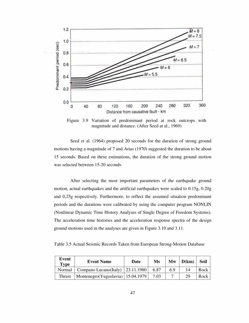
4.5 Saturated and Wet Zones Assumed for the Total Stress Analysis................58
4.6 Shear Modulus and Damping Curves for Clay and Filter Material..............61
4.7 Shear Modulus and Damping Curves for Rockfill Material.........................62
4.8 Shear Wave Velocity Profile of Alluvium Layer.........................................63
4.9 Acceleration Response Spectra at the Base of Dam Body...........................64
5.1 Variation of Fundamental Period with the Peak Ground Acceleration........70
5.2 Location of Nodal Point Numbers Taken for
Acceleration Response Spectra Outputs.......................................................71
5.3 Maximum Acceleration Distribution Throughout the Dam Axis.................72
5.4 Acceleration Response Spectra Along the Centerline of
Akköprü Dam for Synthetic Record 1..........................................................73
5.5 Example of Permanent Displacement Analysis............................................74
5.6 Variation of Permanent Displacement with the
Peak Ground Acceleration............................................................................76
A.1 Earthquakes with M≥4 Occur in Southwestern Anatolia
During the Period 1900-2002.......................................................................89
xvii
LIST OF SYMBOLS
∆σx : Change at the normal stress in x-direction
∆εx : Change at the normal strain in x-direction
∆σxy : Change at the shear stress on xy plane
∆εxy : Change at the shear strain on xy plane
∆σy : Change at the normal stress in y-direction
∆εy : Change at the normal strain in y-direction
σ’1,σ’2, σ’3 : Principal stresses
σ’m : Mean effective stress
α0, α1, α2 : Coefficients for attenuation relationship
�0, �1, �2 : Coefficients for attenuation relationship
βn : Nth root of a period relation
∆W : Dissipated energy
σy : Vertical earth pressure
µ : Damping ratio
ρ : Density
γ : Shear strain
ε : Standard error term
[C] : Global damping matrix
[K] : Global stiffness matrix
[M] : Global mass matrix
A : Constant
aave : Average acceleration
ab : Acceleration of inclined plane
An, Bn : Constants

xviii
arel : Relative acceleration
ay : Yield acceleration
B : Constant
b1, b2, b3 : Coefficients for attenuation relationship
b4, b5, b6 : Coefficients for attenuation relationship
b7, bv : Coefficients for attenuation relationship
d : Closest horizontal distance to the fault
e : Void ratio
E : Young’s modulus
E,F : Moment arms
Fb : Total force acting on sliding block
Fe : Force acting on an element
FS : Factor of safety
g : Gravitational acceleration
G : Shear modulus
GB, GC : Coefficients for attenuation relationship
Gmax : Maximum shear modulus
Gsec : Secant shear modulus
h : Fictitious depth
h : Height of the dam
J0 : Bessel function
K : Bulk modulus
K2 : Parameter relating Gmax and σ’m
Kg : Parameter used for determining maximum shear modulus
kh : Horizontal seismic coefficient
l : Length of sliding surface
M : Moment magnitude
mb : Mass of sliding block
me : Mass of element
Ms : Surface wave magnitude
Mw : Moment magnitude
ng : Exponent used for determining maximum shear modulus

xix
Pa : Atmospheric pressure
r : Closest distance to the source
R : Radius of sliding surface
s : Shear strength
t : Time
u : Displacement
VA : Fictitious shear wave velocity
Vs : Shear wave velocity
W : Maximum strain energy
W : Weight
wn : Nth mode of natural circular frequency
Y : Ground motion parameter
1
CHAPTER I
INTRODUCTION
1.1 General
Water control and assured water availability of appropriate quality become
essential requirements for continuing economic and social development. To satisfy
this, a large number of dams were built all over the world for hydropower generation,
flood control and irrigation. Most of these dams have been located in highly seismic
areas. Many engineers earlier thought that embankment dams had been inherently
safe against earthquakes, but then, especially after the failure of the Lower San
Fernando Dam during San Fernando earthquake 1971, the safety evaluation of the
dams had become a major concern of the engineers.
Results of the studies on the performance of the embankment dams
subjected to strong ground shaking indicate that any well-built dam on a firm
foundation can withstand moderate ground shaking with peak acceleration of about
0.2g, with no detrimental effects. Moreover, dams constructed of clay soils on clay or
rock foundations have withstood extremely strong shaking ranging from 0.35g to
0.8g from a magnitude 8.5 earthquake with no apparent damage. In case of dams
constructed of cohesionless soils, a primary cause of damage or failure is the
build-up of pore water pressures in the embankment and the possible loss of strength
due to high pressures (Seed et al. 1978).

2
There are several ways in which an earthquake may cause failure of an
embankment dam. The most commonly noticed effects are settlement and cracking,
and that may be dangerous depending on their magnitude and location.
Sherard (1967) listed the possible failures of an embankment dam due to earthquake
shaking as follows:
1) Disruption of the dam by major fault movement in foundation.
2) Slope failures induced by ground motions.
3) Piping failure through cracks induced by ground motions.
4) Sliding of dam on weak foundations materials.
5) Loss of freeboard due to differential tectonic ground movements, slope
failures or soil compaction.
6) Overtopping of dam due to seiches in reservoir.
7) Overtopping of dam due to slides or rockfalls into reservoir.
8) Failure of spillway or outlet works.
Considering the potentially harmful effects of earthquakes on embankment dams
Seed (1979) offered the possible defensive measures as follows:
1) Allow ample freeboard to allow for settlement, slumping or fault
movements.
2) Use wide transition zones of material not vulnerable to cracking.
3) Use chimney drains near the central portion of the embankment

3
4) Provide ample drainage zones to allow for possible flow of water
through cracks.
5) Use wide core zones of plastic materials not vulnerable to cracking.
6) Use a well-graded filter zone upstream of the core to serve as a crack
stopper.
7) Provide crest details that will prevent erosion in the event of
overtopping.
8) Flare the embankment core at abutment contacts.
9) Locate the core to minimize the degree of saturation of materials.
10) Stabilize slopes around the reservoir rim to prevent slides into the
reservoir.
11) Provide special details if there is danger of fault movement in the
foundation.
Until circa 1960, the standard method of evaluating the seismic stability of
embankment dams had been the pseudostatic method of analyses which is based on
determining the safety factor of the potential sliding mass, but it gives no information
about the anticipated displacements. In order to estimate the displacements
Newmark (1965) proposed the method of analysis for evaluating the permanent
displacements of embankment dams subjected to strong ground motions. Then, with
the advent of dynamic analysis procedures, the performance of embankment dams
under earthquake loading have been successfully evaluated by using the finite
element method which is extensively used today for design and analysis of the
embankment dams.

4
1.2 Aim of the Study
The aim of this study is to evaluate the response of Dalaman-Akköprü Dam
under earthquake loading with the finite element solutions. As a first step, the
potential sliding mass of the embankment is determined by using the pseudostatic
method. Then, static analysis is performed to obtain the mean effective stresses for
the assessment of the dynamic material properties which represent the nonlinear
behavior of the embankment dam. After this, dynamic analysis is carried out by
employing finite element method with the estimated scenario earthquakes. Finally,
the permanent displacements of the dam under the selected design motions having
different values of peak ground accelerations are determined by using the
acceleration time histories obtained in the dynamic analysis. In order to calculate the
permanent displacements Newmark’s method is used in the analysis.
Chapter 2 reviews the literature and previous studies related with the
evaluation of response of embankment dams. Chapter 3 gives general information
about Akköprü Dam and the seismicity of the site and explains how the design
ground motion is estimated. Chapter 4 describes the steps of the analysis procedures,
how the potential sliding mass is determined, how the static and dynamic analysis are
performed and how the permanent displacements of the potential sliding mass are
calculated. Chapter 5 discusses the results of the analysis and evaluates the dynamic
behavior of the dam. Chapter 6 includes the conclusions of the study.
5
CHAPTER II
STATIC AND DYNAMIC ANALYSES OF EMBANKMENT DAMS
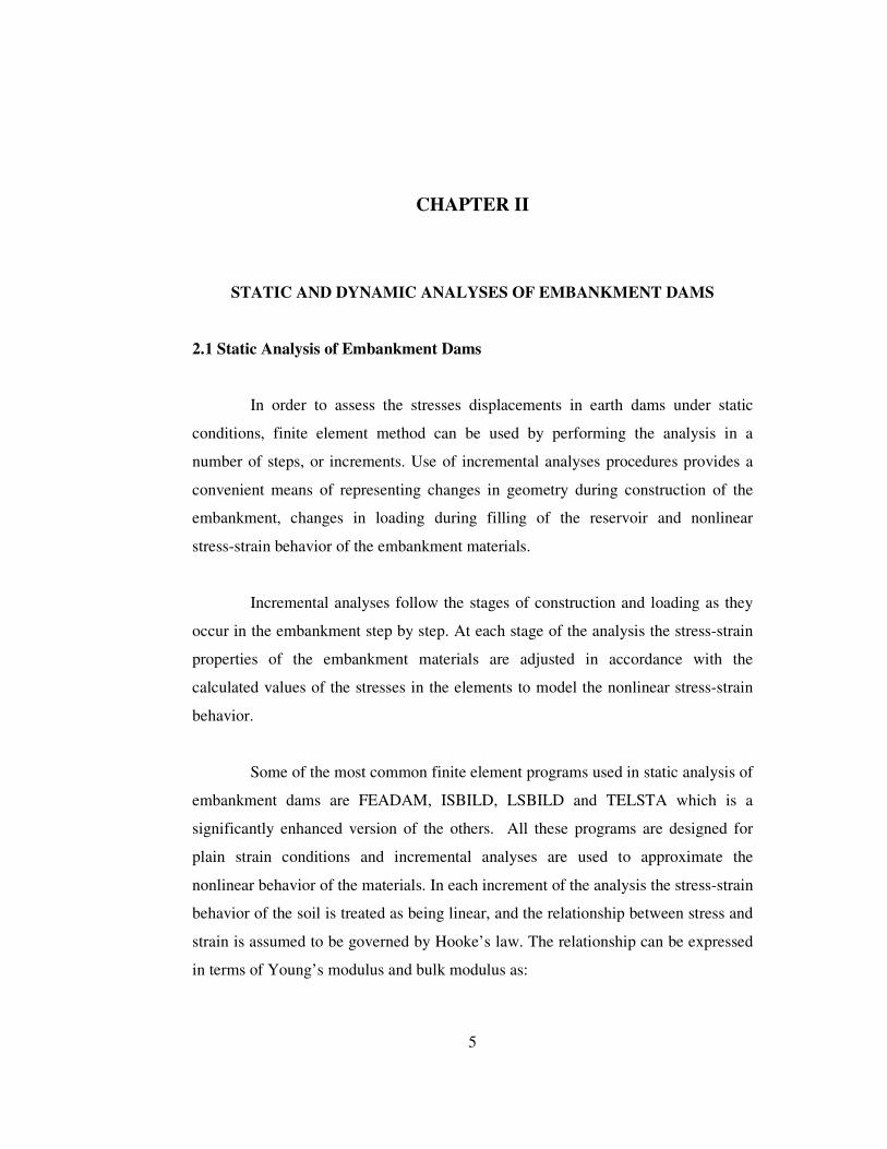
2.1 Static Analysis of Embankment Dams
In order to assess the stresses displacements in earth dams under static
conditions, finite element method can be used by performing the analysis in a
number of steps, or increments. Use of incremental analyses procedures provides a
convenient means of representing changes in geometry during construction of the
embankment, changes in loading during filling of the reservoir and nonlinear
stress-strain behavior of the embankment materials.
Incremental analyses follow the stages of construction and loading as they
occur in the embankment step by step. At each stage of the analysis the stress-strain
properties of the embankment materials are adjusted in accordance with the
calculated values of the stresses in the elements to model the nonlinear stress-strain
behavior.
Some of the most common finite element programs used in static analysis of
embankment dams are FEADAM, ISBILD, LSBILD and TELSTA which is a
significantly enhanced version of the others. All these programs are designed for
plain strain conditions and incremental analyses are used to approximate the
nonlinear behavior of the materials. In each increment of the analysis the stress-strain
behavior of the soil is treated as being linear, and the relationship between stress and
strain is assumed to be governed by Hooke’s law. The relationship can be expressed
in terms of Young’s modulus and bulk modulus as:

6
where ∆σ is the stress, K is the bulk modulus, E is the Young’s modulus and ∆ε is
the strain.
In case of analyses to establish pre-earthquake stresses in an embankment
dam, the deformations are not of interest. A linear finite element program SAP2000
may be used to find the static stresses throughout the dam body. Since the program
does not consider the non-linearity of the soil elements of the dam body, so it will not
give the actual state of stresses within the dam body. Therefore, the iterative
procedure which involves a sequence of calculations is carried out in order to obtain
the actual state of stresses within the dam body. Calculations are related with the
relationship between the elastic modulus of deformation value and the stress value.
In this study, the following equation (2.2) is used suggested by Baba (1982) :
E = A.σyB (2.2)
where E is the elastic modulus of deformation, σy is the vertical stress, A and B are
the constants for core, filter and fill materials of the dam.
2.2 Design Ground Motion
The aim of earthquake resistant design is to produce a structure that can
resists to a certain level of shaking described by a design ground motion. Estimation
of the design ground motion is an essential step of the dynamic analysis of a dam to
determine the acceleration-time history applied at the base of the embankment-
foundation system. In order to select a proper design ground motion for the project
following steps should be investigated:
∆σx 3K 3K+E 3K-E 0 ∆εx ∆σy = 3K-E 3K+E 0 ∆εy (2.1) ∆σxy 9K – E 0 0 E ∆εxy
7
i) Seismicity of the site, seismic risk and past earthquakes (historical
seismicity).
ii) Surface topography, characteristics of the foundation soil and main
rock below the foundation soil and their location.
iii) Type and dynamic material properties of the soil above the main
rock.
iv) Ground motion characteristics at the main rock caused by the
earthquake.
The level of shaking is mostly described in terms of design ground motion
parameters that reflect the characteristics of the design ground motion. The
parameters most commonly used to specify the design ground motion are peak
horizontal acceleration, predominant period and the duration of the earthquake. All
of these parameters are determined in accordance with the estimation of the
magnitude of the maximum credible earthquake which mostly depends on the
historical seismicity of the site.
In case of knowledge of the parameters mentioned above, time history of
the ground motion can be estimated by using several methods. It can be estimated by
using mathematical and statistical methods or calibrating the ground motion
parameters of an actual or synthetic earthquake according to estimated design ground
motion parameters. Since the second approach is simple, it is conventionally used by
the earthquake engineers. In this study, two artificial earthquakes are generated by
using the computer XS artificial earthquake generation program and two actual
earthquakes are used to determine the design ground motion. Furthermore, the
computer program NONLIN (Nonlinear Dynamic Time History Analyses of Single
Degree of Freedom Systems) is used to obtain the desired ground motion parameters
reflecting the characteristics of the design ground motion.

8
2.2.1 Estimation of Peak Ground Acceleration
For the assessment of peak ground acceleration a number of predictive
relationships in other words attenuation relationships have been developed. These
relationships involve the earthquake magnitude, type of faulting, distance to fault and
site conditions. They are developed by regression analyses of recorded strong ground
motion databases. When using any predictive relationship, it is very important how
parameters such as M (magnitude) and R (distance to fault) defined and use of them
in a consistent manner. It is also important to recognize that different predictive
relationships are usually obtained from different data sets.
Attenuation relationships used in this study are given below.
I.M. Idriss (1991) suggested the following empirical relationship:
Ln(Y) = [α0 + exp(α1 + α2M)] + [�0 – exp(�1 + �2M)]Ln(R + 20) + 0.2 F + � (2.3)
For M � 6 α0 = -0.150, α1 = 2.261, α2 = -0.083, �0 = 0, �1 = 1.602,
�2 = -0.142 and � = 1.39 – 0.14M
For M > 6 α0 = -0.050, α1 = 3.477, α2 = -0.284, �0 = 0, �1 = 2.475,
�2 = -0.286 and � = 1.39 – 0.14M
Ln : natural logarithm
exp : exponential function
Y : ground motion parameter (peak horizontal acceleration, a in g’s,
and pseudo absolute spectral acceleration, at 5%damping)
M : local magnitude, ML, for M � 6 and surface wave magnitude, MS
for M>6. Thus, in essence, M represents moment magnitude, Mw.
R : closest distance to the source in km; however, for M � 6 the
hypocentral distance is used.
F : style of faulting factor; F=0 for a strike slip fault; F=1 for a
reverse fault and F=0.5 for an oblique source.

9
� : standard error term.
Boore et al(1993). proposed the following relationship:
Log (Y) = b1 + b2(M-6) + b3(M-6)2 + b4r + b5logr + b6 GB + b7GC (2.4)
where r = (d2 + h2)1/2, d is the closest distance to the surface projection of the fault in
kilometers, Y is the peak ground acceleration in g, M is the moment magnitude, for
randomly-oriented horizontal component (or geometric mean) b1 = -0.105,
b2 = 0.229, b3 = 0, b4 = 0, b5 = -0.778, b6 = 0.162, b7 = 0.251, h=5.57 and σ = 0.230
(for geometrical mean σ = 0.208) and for larger horizontal component b1 = -0.038,
b2 = 0.216, b3 = 0, b4 = 0, b5 = -0.777, b6 = 0.158, b7 = 0.254, h=5.48 and σ = 0.205
and
For site class A, Vs,30 > 750 m/sec, GB = 0, GC =0
For site class B, 360 < Vs,30 < 750m/sec, GB = 1, GC =0
For site class C, 180 < Vs,30 < 360m/sec, GB = 0, GC =1
Kalkan (2001) estimated the following attenuation relationship for Turkey
sites by using the same general form of the equation proposed by Boore et al. (1997).
Ln(Y) = b1 + b2(M-6) + b3(M-6)2 + b5lnr + bv(ln Vs / VA) (2.5)
where r = (d2 + h2)1/2, Y is the peak ground acceleration, M is the moment
magnitude, d is the closest horizontal distance from the station to a site of interest in
km, VA is the fictitious shear wave velocity, Vs is shear wave velocity in m/sec, and
b1 = -0.682, b2 = 0.253, b3 = 0.036, b5 = -0.562, bv = -0.297, VA = 1381 m/s,
h = 4.48 and σ = 0.562
10
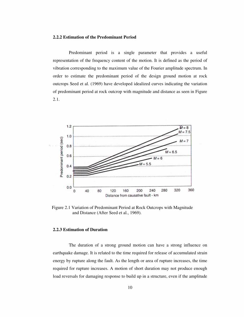
2.2.2 Estimation of the Predominant Period
Predominant period is a single parameter that provides a useful
representation of the frequency content of the motion. It is defined as the period of
vibration corresponding to the maximum value of the Fourier amplitude spectrum. In
order to estimate the predominant period of the design ground motion at rock
outcrops Seed et al. (1969) have developed idealized curves indicating the variation
of predominant period at rock outcrop with magnitude and distance as seen in Figure
2.1.
2.2.3 Estimation of Duration
The duration of a strong ground motion can have a strong influence on
earthquake damage. It is related to the time required for release of accumulated strain
energy by rupture along the fault. As the length or area of rupture increases, the time
required for rupture increases. A motion of short duration may not produce enough
load reversals for damaging response to build up in a structure, even if the amplitude
Figure 2.1 Variation of Predominant Period at Rock Outcrops with Magnitude and Distance (After Seed et al., 1969).

11
Figure 2.2 Illustration of Bracketed Duration for 0.05g Threshold Acceleration (Kramer 1996)
of motion is high. On the other hand a motion with moderate amplitude but long
duration can produce load reversals to cause substantial damage.
An earthquake accelerogram generally contains all accelerations from the
time the earthquake begins until the time the motion has returned to the level of
background noise. For engineering purposes, only the strong motion portion of the
accelerogram is of interest. Different approaches have been taken to the problem of
evaluating the duration of strong motion in an accelegrogram. The bracketed
duration (Bolt 1969) is defined as the time between the first and last exceedances of a
threshold acceleration (usually 0.05g). Based on a threshold acceleration of 0.05g,
the bracketed durations can be obtained from the accelerogram as shown in Figure
2.2.
The duration of strong motion has been investigated by interpretation of
accelegrograms from earthquakes of different magnitudes. By using a 0.05g
threshold acceleration, Chang and Krinitszky (1977) estimated the bracketed
durations for soil and rock sites at short (less than 10 km) epicentral distances shown
in Table 2.1. Another definition of duration (Trifunac and Brady, 1975b) is based on
the time interval between the points at which 5% and 95% of the total energy has

12
been recorded. Boore (1983) has taken the duration to equal to corner period. The
rate of change of cumulative root-mean-square (rms) acceleration has also been used
as the basis for evaluation of strong-motion duration (McCann and Shah, 1979).
Among these definitions, the bracketed duration is most commonly used for
earthquake engineering purposes because it implicitly reflects the strength of shaking
(Kramer 1996).
Table 2.1 Typical Earthquake Durations at Epicentral Distances less than 10 km
Duration (sec) Magnitude
Rock Sites Soil Sites
5.0 4 8
5.5 6 12
6.0 8 16
6.5 11 23
7.0 16 32
7.5 22 45
8.0 31 62
8.5 43 86
2.3 Dynamic Analysis of Embankment Dams
2.3.1 Pseudostatic Method of Analysis
The seismic safety of earth structures has been analyzed for almost seventy
years by using the method of pseudostatic analysis. In this method the same principle
is used as in the static slope stability analyses and the overturning and resisting
forces on the critical slope surface are taken into consideration. The earthquake
effects are represented by an earthquake static horizontal force determined by a
seismic coefficient k and the weight of the sliding mass as seen in Figure 2.3.
Equivalent horizontal force can be formulated as follows:

13
Figure 2.3 Forces Acting on the Potential Circular Sliding Mass in Pseudostatic Method
Feq = kh * W ( 2.6)
By using a simple moment equilibrium analyses the factor of safety can be
defined as the ratio resists rotation of a critical slip surface about the center of the
sliding surface to the moment that is driving the rotation. For a circular sliding
surface as seen in Figure 2.3, the factor of safety can be formulated as follows:
where as the shear strength, weight and seismic coefficient are denoted by s, W and
kh, respectively. O is the center of the sliding circle and O1 is the gravity center of
Resisting Moments s*l*R FS = = (2.7) Overturning moments E*W + kh *F*W

14
the sliding mass; E and F are the moment arms; and R and l are radius and length of
the sliding surface respectively.
Equation (2.6) is based on the simplifying assumptions that the horizontal
acceleration khg acts permanently on the slope material and in one direction only.
Therefore, the concept in conveys of earthquake effects on slopes is very inaccurate
to say the least. Theoretically, a value of FS = 1 would mean a slide, but in reality a
slope may remain stable in spite of FS being smaller than unity and it may fail at a
value of FS>1 depending on the character of the slope forming material
(Terzaghi 1950). This statement clearly indicates that a slope may be unstable even if
the FS is greater than 1. Related to this case some of the major slope failures of dams
analyzed with pseudostatic method are listed in Table 2.2.
As seen from the cases in Table 2.2, in pseudostatic analyses the most
important difficulty is the selection of an appropriate seismic coefficient. The seismic
coefficient mostly depends on the seismicity activity of the region, type of the dam
embankment material and the importance of the project. For the selection of seismic
coefficient Seed (1979) listed pseudo design criteria for 14 dams in 10 seismically
active countries; 12 required minimum factor of safety of 1.0 to 1.5 with pseudostatic
coefficients of 0.10 to 0.12. Marcuson (1981) suggested that appropriate pseudostatic
coefficients for dams should correspond to one-third to one half of the maximum
acceleration, including amplification and deamplification effects, to which the dam is
subjected. Seed (1979) also indicated that deformations of earth dams constructed of
ductile soils with crest accelerations less than 0.75g would be acceptably small for
pseudostatic factors of safety of at least 1.15 with kh=0.10 (M=6.5) to kh=0.15
(M=8.25). This criteria would allow the use of pseudostatic accelerations as small as
13 to 20 % of the peak crest acceleration (Kramer 1996).
As a conclusion, difficulties in the selection of seismic coefficients and in
the evaluation of safety factor have reduced use of pseudostatic method for seismic
slope stability analyses. Hence, today finite element method has become reliably
possible to investigate the behavior of embankment dams under earthquake loading.

15
Table 2.2 Pseudostatic Analyses of Dams with Slope
Failures During Earthquakes (Seed 1979)
Dam Seismic
coefficient
Computed
factor of safety
Effect of earthquake
Sheffield Dam 0.1 1.2 Complete failure
Lower San Fernando
Dam
0.15 1.3 Upstream slope failure
Upper San Fernando
Dam
0.15 ≈2 to 2.5 Downstream shell including
crest slipped about 6ft
downstream
Tailings Dam (Japan) 0.2 ≈1.3 Failure of dam with release of
tailings
2.3.2 Shear Beam Method
Dynamic response analysis of the two dimensional earth dams can be
greatly simplified by the shear beam analysis. It allows two dimensional problem to
be modeled as equivalent one dimensional problem by using the following
assumptions:
i) The dam is infinitely long and it consists of homogeneous and linearly
elastic material.
ii) The dam moves only at horizontal direction. Only horizontal shear
deformations are considered
iii) Shear stresses or shear strains are uniform across horizontal planes.

16
∂ 2u G ∂ 2u 1 ∂ u = + (2.8) ∂ t2 ρ ∂ z2 z ∂z
iv) The dam consists of thin horizontal slices. These slices are connected to
each other with elastic springs and viscous damping mechanisms.
v) Influence of the reservoir is neglected.
Based on the assumptions above the dam body can be illustrated as in
Figure 2.4 and the dynamic equilibrium can be represented as follows:
where u is the horizontal displacement at a given depth z, t is the time, G is the shear
modulus and ρ is the mass density of the construction material. Using the boundary
conditions u=0 at z=h and ∂ u/ ∂ z=0 at z=0 the solution of the differential equation is
obtained as follows:
where h is the height of the dam, An and Bn are the constants, J0 is the Bessel
function of first kind of zero and βn is the n-th root of period relation for the modes
(β1=2.404, β2=5.520, β3=8.654, β4=11.792, β5= 4.931 etc.), wn is the n-th mode of
natural circular frequency which may be written as:
βn wn = Vs (2.10) h
∞ y u(z,t) = � [Ansinwnt+Bncoswnt] J0 (βn ) (2.9) n=1 h

17
Figure 2.4 Earth Dam, Showing Stresses Acting on an Element of Thickness, dz
where Vs is the shear wave velocity. Substituting wn = 2π/T and Bn values into
Equation 2.10, natural periods for two modes of vibration are obtained as:
T1 = 2.612 h/ Vs (2.11)
T2 = 1.138 h/ Vs (2.12)
These equations give better results when the rate of width of the base of the
dam to the height of the dam is almost three.
Consequently, in the shear beam method earthquake induced accelerations
and deformations acting only in horizontal direction can be determined. It is
fundamentally different from the equivalent linear and non-linear models in that it
restricts particle movement to the horizontal plane. Even though the shear beam
analysis gives general idea about the dynamic behavior of an earth dam, due to the
restrictions and assumptions explained above it is far from reflecting actual results.
18
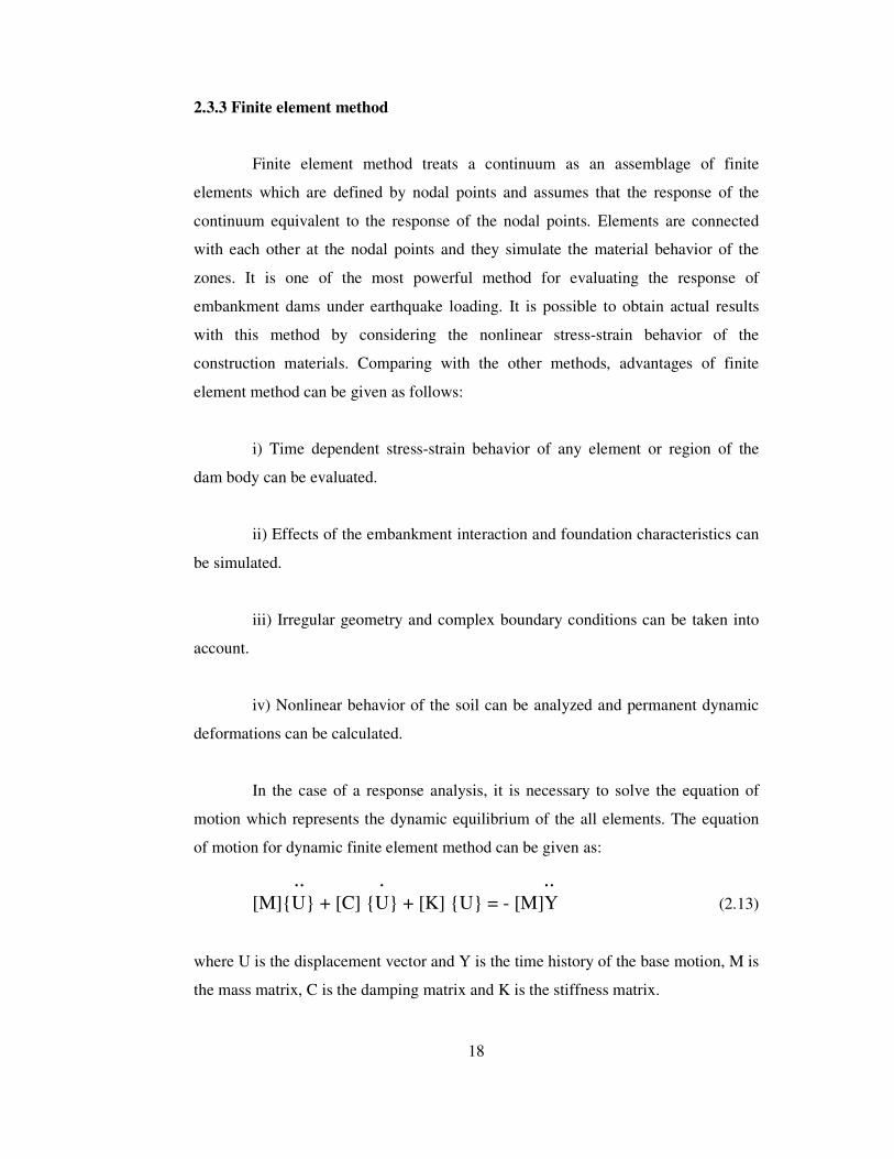
2.3.3 Finite element method
Finite element method treats a continuum as an assemblage of finite
elements which are defined by nodal points and assumes that the response of the
continuum equivalent to the response of the nodal points. Elements are connected
with each other at the nodal points and they simulate the material behavior of the
zones. It is one of the most powerful method for evaluating the response of
embankment dams under earthquake loading. It is possible to obtain actual results
with this method by considering the nonlinear stress-strain behavior of the
construction materials. Comparing with the other methods, advantages of finite
element method can be given as follows:
i) Time dependent stress-strain behavior of any element or region of the
dam body can be evaluated.
ii) Effects of the embankment interaction and foundation characteristics can
be simulated.
iii) Irregular geometry and complex boundary conditions can be taken into
account.
iv) Nonlinear behavior of the soil can be analyzed and permanent dynamic
deformations can be calculated.
In the case of a response analysis, it is necessary to solve the equation of
motion which represents the dynamic equilibrium of the all elements. The equation
of motion for dynamic finite element method can be given as:
.. . .. [M]{U} + [C] {U} + [K] {U} = - [M]Y (2.13) where U is the displacement vector and Y is the time history of the base motion, M is
the mass matrix, C is the damping matrix and K is the stiffness matrix.

19
There are several methods used for the solution of the Equation 2.13. These
methods can be written as:
i) Direct Integration
ii) Modal Superposition
iii) Fourier Analysis
The most common method used for evaluating the behavior of non-linear
systems under cyclic loading is the direct integration method. The other methods;
modal superposition and Fourier analysis are only valid for the evaluation of the
linear-elastic systems.
The finite element method can be used for the solution of the two
dimensional and three dimensional dynamic response problems. In the case of earth
structures, usually plane strain and two dimensional analysis of transverse (along the
river valley, normal to dam axis) sections are used. There are several computer
programs available involving the assumption of plain strain conditions. Some of the
computer programs used for the evaluation of the response of embankment dams are
QUAD-4 (Idriss et al, 1973), LUSH (Lysmer et al, 1974), FLUSH (Lysmer et al,
1975) and TELDYN (Pyke et al, 1984). Among them, an effective one is TELDYN
which uses equivalent linear method, provides compliant base and determines the
excess pore water pressures.
2.4 Equivalent Linear Model
In case of earthquake response analyses, properties of soils under dynamic
conditions are nonlinear and hysteretic. The equivalent linear model has been most
widely used for the representation of this nonlinear behavior in embankment and
foundation soils. Shear stress-shear strain relationships for soils subjected to cyclic
loading are nonlinear and exhibit hysteresis loop of the type as shown in Figure 2.5.
As can be seen from the Figure 2.5 the average (equivalent linear) shear modulus can
be represented by the secant modulus drawn through the ends of the hysteresis loops.

20
As the cyclic shear strain amplitude increases, the average shear modulus decreases
and the hysteretic damping, as indicated by the area enclosed by the shear strain
curve increases.
Instead of hysteretic damping, equivalent damping ratio can be described by
using the following formula :
where ∆W is the dissipated energy represented by the area of hysteresis loop, W is
the maximum strain energy represented by the area of the OAB triangle.
As explained above secant shear modulus of the soil element varies with
cyclic shear strain amplitude. At low strains, the secant shear modulus (Gsec) is high,
but it decreases as the shear strain amplitude increases. This variation of Gsec with
cyclic shear strain can be shown with a curve called backbone as seen in Figure 2.6.
In the figure tangent modulus at the origin represents the largest value of shear
modulus (Gmax), γc is the current strain and Gsec (hereafter instead of Gsec only G is
used for notation) is the corresponding shear modulus. From the backbone curve the
modulus reduction curve indicating the variation of G / Gmax ratio with shear strain
can be determined as shown in Figure 2.7.
In the early years of geotechnical earthquake engineering, Seed and
Idriss (1970) suggested modulus reduction curves and damping curves for coarse and
fine-grained soils. Then, Seed (1984) and the other researches such as Hardin and
Drnevich (1972), Vucetic and Dobry (1991), Ishibashi (1992) modified the curves
according to mean effective stress and plasticity index. The curves commonly used
for cohesionless soils proposed by Seed (1984) and for cohesive soils proposed by
Vucetic and Dobry (1991) can be seen in Figure 2.8 and 2.9 respectively.
1 ∆W µ = (2.14) 4π W

21
Figure 2.5 Hysteric Loop Indicating Shear Stress Relationship for Soils Subjected to Cyclic Loading

22
Figure 2.6 Backbone Curve Showing Typical Variation of Gsec with Shear Strain
Figure 2.7 The Variation of the Modulus Ratio with Shear Strain

23
Figure 2.8 Modulus Degradation and Damping Curves for Cohesionless Soils (Seed et al. 1984)

24
Figure 2.9 Modulus Degradation and Damping Curves for Cohesive Soils (Vucetic & Dobry 1991)
25
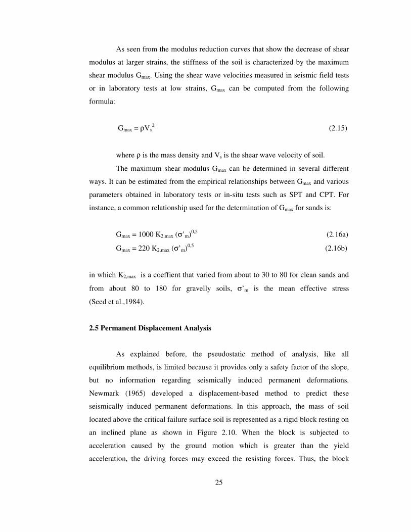
As seen from the modulus reduction curves that show the decrease of shear
modulus at larger strains, the stiffness of the soil is characterized by the maximum
shear modulus Gmax. Using the shear wave velocities measured in seismic field tests
or in laboratory tests at low strains, Gmax can be computed from the following
formula:
Gmax = ρVs2 (2.15)
where ρ is the mass density and Vs is the shear wave velocity of soil.
The maximum shear modulus Gmax can be determined in several different
ways. It can be estimated from the empirical relationships between Gmax and various
parameters obtained in laboratory tests or in-situ tests such as SPT and CPT. For
instance, a common relationship used for the determination of Gmax for sands is:
Gmax = 1000 K2,max (σ’m)0,5 (2.16a)
Gmax = 220 K2,max (σ’m)0,5 (2.16b)
in which K2,max is a coeffient that varied from about to 30 to 80 for clean sands and
from about 80 to 180 for gravelly soils, σ’m is the mean effective stress
(Seed et al.,1984).
2.5 Permanent Displacement Analysis
As explained before, the pseudostatic method of analysis, like all
equilibrium methods, is limited because it provides only a safety factor of the slope,
but no information regarding seismically induced permanent deformations.
Newmark (1965) developed a displacement-based method to predict these
seismically induced permanent deformations. In this approach, the mass of soil
located above the critical failure surface soil is represented as a rigid block resting on
an inclined plane as shown in Figure 2.10. When the block is subjected to
acceleration caused by the ground motion which is greater than the yield
acceleration, the driving forces may exceed the resisting forces. Thus, the block

26
slides along the inclined plane. The resisting and the driving forces acting on the
sliding block are illustrated in Figure 2.11.
Determination of the yield acceleration is the most critical step of the
analysis. The yield acceleration ay is the minimum pseudostatic acceleration required
to cause the block to move relative to sliding plane. It can be obtained by using the
following equation:
ay = kh . g (2.17)
where kh is the horizontal seismic coefficient calculated in pseudostatic analysis
which is explained in Section 2.3.1.
When a block on an inclined plane is subjected to accelerations greater than
the yield acceleration, the block will move relative to plane. Thus, the relative
acceleration occurring the displacement can be written as follows:
arel(t) = ab(t) - ay (2.18)
where ab(t) is the acceleration of inclined plane.
Thus, by computing an acceleration at which the inertia forces become
sufficiently high to cause yielding to begin and integrating the effective acceleration
on the sliding mass in excess of this yield acceleration as a function of time (Figure
2.12), the velocities and ultimately displacements of the slide mass could be
evaluated (Seed et al.,1979).
The time history acceleration of the inclined plane, ab(t), can be considered
as the average time history acceleration of the sliding mass. In order to determine the
average time history acceleration, aave, following steps should be carried out:

27
Figure 2.10 Sliding Block Resting on an Inclined Plane
α W
N
N tanφ kW
Figure 2.11 Forces Acting on the Sliding Block

28
i) Sliding mass is divided into finite elements or finite strips.
ii) The average time history of acceleration is calculated for each element by
using the dynamic finite element analysis.
iii) The time history of force on an element is obtained by multiplying the
acceleration of each element with its mass:
Fe(t) = me.ae(t) (2.19)
where me is the mass of an element and ae(t) is the time history of acceleration of an
element.
iv) Total force acting on the sliding mass can be calculated by summing the
forces acting on elements:
Fb(t) = � Fe(t) = � me.ae(t) (2.20)
v) In the last step, the average time history acceleration of the sliding mass
is determined by dividing total force by total mass of the sliding mass:
Consequently, as explained before, by integrating twice average time history
of acceleration, permanent displacement of the slope can be calculated.
Makdisi and Seed (1978) developed the Newmark’s permanent
displacement method by using the sliding block analyses and average accelerations
computed by the procedure of Chopra (1966). In this approach, knowing the
Fb(t) � me.ae(t) aave = = (2.21) mb � me .

29
fundamental period of embankment and the yield acceleration of the slope, simple
charts can be used to estimate earthquake-induced permanent displacements.
Furthermore, Lemos and Coelho (1991) and Tika Vassilikos et al. (1993) have both
suggested methods that can incorporate a rate dependent friction angle into the
Newmark analysis to account for time varying shear strengths due to earthquake
loading. Although a number of modified permanent displacement methods have been
proposed, today Newmark (1965) type of analysis is widely used by the geotechnical
engineers.

30
Figure 2.12 Integration of Effective Acceleration Time-History to Determine Velocities and Displacements
(Seed et al., 1979)

31
CHAPTER III
AKKÖPRÜ DAM AND SEISMICITY OF THE SITE
3.1 General Information About Dalaman - Akköprü Dam
Dalaman-Akköprü Dam is a rockfill dam located at Dalaman Basin in the
southwest of Aegean Region, being built on the Dalaman River, 24 km east of the
Köyce�iz Town in Mu�la. Construction of the dam was started in 1995 and it is
planned to be completed in 2005. The main purposes of this project are the
hydropower generation, irrigation and flood control. The general view of Akköprü
Dam is given in Figure 3.1. (DS�, 2003)
3.1.1 Characteristics of the Project
Dam Reservoir Data
Rainfall area : 5132.60 km2
Annual average of water : 1627.40 hm3
Regulated water : 849.70 hm3
Regulation : 52 %
Minimum water level : 173.50 m
Normal water level : 200.00 m
Maximum water level : 204.00 m (In flood)
Minimum water level volume : 195.81 hm3
Normal water level volume : 384.50 hm3
Maximum water level volume : 419.20 hm3
Maximum reservoir area : 8.92 km2

32
Figu
re 3
.1 P
hoto
of A
kköp
rü D
am T
aken
at t
he e
nd o
f yea
r 200
3

33
Dam Embankment Data
Type : Rock-fill with clay core
Crest elevation : 207.50 m
Crest length : 688.70 m
Crest width : 12.00 m
Height from thalweg : 112.50 m
Height from foundation : 162.50 m
Total body volume : 12.50 hm3
Spillway Data
Type : Radial gate, 4 gates
Dimensions of the gate : 11.60 x 15.71 m
Spillway top elevation : 188.50 m
Spillway design flood : 5730.00 m3 / s
Discharge channel length : 445.37 m
Hydroelectric Power Plant (Powerhouse)
# of Units : 2 Units
Turbine type : Vertical axis Francis
Unit capacity : 57.5 MW
Installed capacity : 115 MW
Rated head : 101 m
Design discharge : 150 m3 / s
# of cycles of the unit : 250 rpm
Annual energy production : 343.5 GWh

34
Diversion Tunnels
Tunnel diameter : 6.50 m
Length - Derivation tunnel 1 : 766.62 m
Length - Derivation tunnel 2 : 808.44 m
Bottom Outlet
Type : Circular 2 pieces
Length : 315.50 m (for both tunnels)
# of Danger valve : Slide valve, 1 piece, 180 cm x 180 cm
type and dimension (for both tunnels)
# of Adjusting valve, : Conic valve, 1 piece, 200 cm
type and dimension (for both tunnels)
Bottom outlet capacity : 145.44 m3 / s
Energy (Power) Tunnel
Tunnel diameter : 6.50 m
Length : 532.00 m
Vertical shaft length : 72.00 m
Penstock
Pipe diameter : 6.45 – 3.23 m
Length : 204.00 m
3.1.2 Geology and the Foundation
The base rock at the Akköprü Dam site is peridotite-serpantine. This unit is
generally impermeable. Some parts are semi-pervious and 60 m deep grout curtain

35
beneath the foundation dam upstream and downstream cofferdam axis were
constructed by slurry trench method.
Alluvium thickness of the dam site is 38 m. Alluvium is permeable and it
was excavated prior to the construction of the dam.
At right abutment 37.20 m thick terrace deposits were observed and
excavated.
The base rock at the reservoir area is composed of autochthonous Akta�
limestone and Gökseki flysch formation. Allochtononous Cehennem limestone and
Demirli complex serie (melange) overlay autochthon units. Akta� limestone and
Cehennem limestone formations are permeable. The karstification base and
discharge points in Cehennem limestone are located over maximum water level. So,
no big problems related to leakage and seepage are expected from this unit
(�ekercio�lu et al., 1999).
Akta� limestone is very permeable and groundwater level elevation is
located around 116 m below the Dalaman river. In order to prevent leakage from
Akta� limestone , concrete blanket is planned to be constructed.
3.1.3 The Dam Embankment
Akköprü Dam is a rockfill dam having a large clay core, sand and gravel
filter zones. The plan view and the maximum cross section of the embankment can
be seen in Figure 3.2 and 3.3 respectively. The height of the dam is 162.50 m from
the lowest foundation level and 112.50 m from the thalweg. Its crest is 688.70 meters
long and 12.00 meters wide. The total dam body volume is 12.30 hm3. Downstream
slope of the dam is 1(V) / 2(H) and upstream slope of the dam is 1 (V) / 2.5 (H).
The main properties of the materials used at the construction of the dam
body as provided by State Hydraulic Works (DS�) are given in Table 3.1.

36
Figu
re 3
.2 P
lan
Vie
w o
f Akk
öprü
Dam

37
Figu
re 3
.3 C
ross
Sec
tion
of A
kköp
rü D
am

38
Table 3.1 Properties of Dam Embankment Material
Material Type Dry
Density
Wet
Density
Saturated
Density
Angle of
Friction
(φφφφ�
Cohesion
Undrained
(C�
kN/m3 kN/m3 KN/m3 (º) kN/m2
Core Material
Clay (CL)
16.5 19.7 20.4 20 40
Grade Filter
Material
17.5 18.5 21.5 33 0
Fill material
Rock
19.5 20.0 21.0 43 0
Subbase material
Alluvium
16.6 17.4 20.2 33 0
Base material
Rock
23.0 23.0 23.0 25 20
3.2 Seismicity of Akköprü Dam Site
Akköprü Dam is located at southwest of Aegean Region and Eastern
Mediterranean Sea. The important normal faults in Turkey exist in the West
Anatolia. These faults form the graben system and indicate the deformation
continuity occurring in the Aegean-Western Anatolia plate.
There is a wide earthquake zone near the Aegean Sea and Eastern
Mediterranean Sea Earthquakes of both shallow focal depth (50 km<h) and mid focal
depth (50 km< h < 200 km) (Alptekin 1978). Investigations made by State Hydraulic
Works (DS�) in this earthquake zone indicate that there are four main regions:
- 1st region includes the west and southwest of the Datça Peninsula.
- 2nd region includes Köyce�iz, Ula, Çameli, Fethiye and Dalaman

39
- 3rd region includes Acı Lake, Burdur Lake and Söke
- 4th region includes Aydın, Denizli and Burdur.
Tectonic map of the earthquake zone including four regions stated above
investigated by DS� is shown in Figure 3.4. Furthermore macro seismic maps of
Fethiye Earthquake, Aegean – Mediterranean Earthquake are given in Figure 3.5 and
3.6, respectively.
It is observed that 770 earthquakes with magnitudes greater than 4.0 have
occurred in the region bounded by 35.00º - 38.00º N and 27.00º - 30.00º E during the
period 1900 – 2002. Epicenter map of the earthquakes with magnitudes greater than
4.0 and a list of the earthquakes with their occurring dates, epicenter locations, focal
depths and magnitudes are given in Appendix A.
3.3 Design Earthquake Ground Motion
The procedures employed and the results are obtained in the assessment of
engineering parameters of ground motion at the site are presented in this section.
First the results of probabilistic studies performed earlier are reviewed. Next the
deterministic studies carried out to estimate the peak ground motion parameters are
summarized.
3.3.1 Probabilistic Assessment
Yaralıo�lu et al. (1982) had studied the seismicity of the region around
Akköprü dam site. In this work to find the acceleration-risk values an investigation
region is selected between the geographical coordinates 36º00 - 38º00 N and
27º00 - 32º00 E and a tectonic map of the region is prepared as seen in Figure 3.4
(Yaralıo�lu et al., 1982). On this map major sismotectonic features of the region are
idealized as a line and three area sources as seen in Figure 3.4.

40
.
Figu
re 3
.4 T
ecto
nic
Map
of t
he E
arth
quak
e Z
one
Surr
ound
ing
the
Akk
öprü
Dam
Site
(Y
aral
ıo�l
u et
al.,
198
2)

41
Figure 3.5 Macroseismic map of 1957 Fethiye Earthquake ( Ergin et al., 1967)
Figure 3.6 Macroseismic map of 1961 Aegean –Mediterranean Earthquake ( Ergin et al., 1967)

42
Based on this seismotectonic model Yaralıo�lu et al. (1982) had performed
a Cornell-type seismic risk analysis in terms of peak ground acceleration. The
attenuation relationships developed by Esteva (1970) had been employed in the
analysis which did not take into account the effects of the local site conditions at
recording stations.
Summary of this results of seismic risk analysis by Yaralıo�lu et al. (1982)
are given in Table 3.2, 3.3 & Figure 3.8, 3.9.
Probability of
exceedence 0.05 0.10 0.20
Economic Life Peak Ground Acceleration cm/sn2
1 year 72.5 48.7 43.5
50 years 296 253.7 200.5
100 years 352.2 294.7 249.7
1000 years 666.1 511.7 389.7
PGA(cm/s2) 10 50 100 150 200 250 300 400 500 1000
Economic
Life Probability of exceedence of Peak Ground Acceleration (PGA) %
1 year 85 7.7 1.95 0.87 0.43 0.22 0.09 0.014 0.08 0.0014
50 years 100 98 69 35 19 10 4.5 0.7 0.42 0.08
100 years 100 99.9 86 58 35 10 8.5 1.45 0.83 0.15
1000 years 100 100 100 99.9 98 88 60 13 7. 1.64
Table 3.2 Expected Peak Ground Acceleration Values at Akköprü Dam Site
Table 3.3 Probability of exceedence of PGA at Akköprü Dam Site
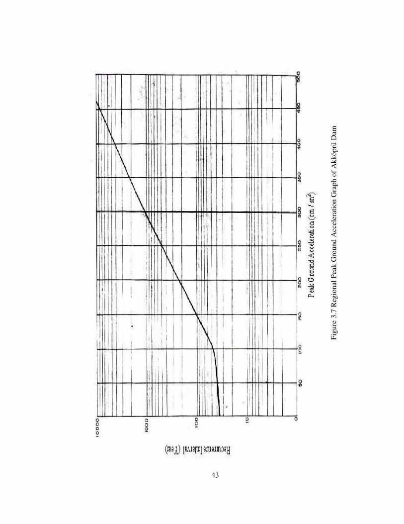
43
Figu
re 3
.7 R
egio
nal P
eak
Gro
und
Acc
eler
atio
n G
raph
of A
kköp
rü D
am

44
Figu
re 3
.8 E
quip
oten
tial A
ccel
erat
ion
Cur
ves
of A
kköp
rü D
am w
ith 2
0 %
Pro
babi
lity
of E
xcee
denc
e fo
r 100
Yea
r Eco
nom
ic L
ife

45
3.3.2 Deterministic Assessment
The seismicity of the region had been fully investigated in the probability
studies by Yaralıo�lu et al. (1982). The map in Figure 3.4 indicates the main tectonic
features of the region under consideration. The largest event for this period was
25.04.1957 Fethiye Earthquake which has a magnitude of about 7. The details of the
seismicity may be found in the references cited.
From the results of probabilistic studies and the seismotectonic features of
the region, it is concluded that a large magnitude event occurring in fault near
Marmaris would govern the design earthquake ground motions at the site of Dalaman
Akköprü Dam.
For an assessment of design earthquake motion parameters, an earthquake
having a large magnitude of M=7 is considered. The distance to the causative fault is
assumed to be 28 km.
3.3.2.1 Acceleration – Attenuation Approach
Estimation of ground motion parameters for a certain location at a given
distance from the epicenter or the causative fault of an earthquake are made by the
use of empirical relationships. Attenuation relationships that express ground motion
parameters as a function of magnitude, distance, type of faulting and site conditions.
The most commonly used ground motion parameter is PGA (Peak Ground
Acceleration). In order to estimate the PGA value at Akköprü Dam site Idriss et al.
(1991), Boore et al.(1993) and Kalkan (2001) attenuation relationships explained in
Chapter II are used . Magnitude and the distances are selected as stated above. Local
soil conditions and type of faulting are also necessary. The geology of the dam site
generally consists of rock formations.
46
The results of the acceleration attenuation approach of the deterministic
study are tabulated as follows in Table 3.4.
Table 3.4 Expected Peak Ground Acceleration Values at Dam Site
PGA for Mw=7.0 and R=28 km
Idriss (1991) 0.160g
Boore (1993) 0.112g
Kalkan(2001) 0.086g
3.4 Design Peak Ground Acceleration
In the probabilistic assessment peak ground acceleration was determined as
approximately 0.25g with the probability of 20 % exceedence in 100 years which is
equivalent to occurrence of once in 450 years. In the deterministic assessment from
attenuation relationships by Idriss (1991), Boore (1993) and Kalkan (2001) the peak
ground accelerations were calculated as 0.160g, 0.112g and 0.086g respectively.
According to these results design peak ground acceleration was selected as 0.20g.
3.5 Estimating Input Ground Motion
There are no actual earthquake motion records available at the project site.
Hence, in order to make dynamic analyses of Akköprü Dam, two actual earthquakes
taken from European Strong Motion Database were used and given in Table 3.5 and
two synthetic earthquake motions were generated by XS artificial motion generation
program. Based on the historical seismic events at the dam site the maximum
probable earthquake magnitude of Mw=7 was estimated for the analyses. The most
important parameters of the earthquake hazard motion are the peak ground
acceleration, predominant period (frequency content) and the duration of the
earthquake. As mentioned before, the most critical fault is at a distance of 28 km
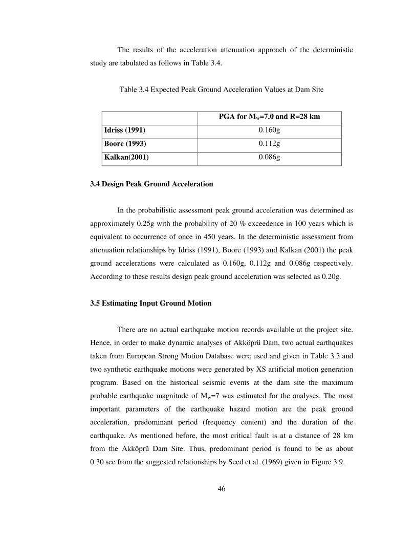
from the Akköprü Dam Site. Thus, predominant period is found to be as about
0.30 sec from the suggested relationships by Seed et al. (1969) given in Figure 3.9.
47
Seed et al. (1964) proposed 20 seconds for the duration of strong ground
motions having a magnitude of 7 and Arias (1970) suggested the duration to be about
15 seconds. Based on these estimations, the duration of the strong ground motion
was selected between 15-20 seconds.
After selecting the most important parameters of the earthquake ground
motion, actual earthquakes and the artificial earthquakes were scaled to 0.15g, 0.20g
and 0,25g respectively. Furthermore, to reflect the assumed situation predominant
periods and the durations were calibrated by using the computer program NONLIN
(Nonlinear Dynamic Time History Analyses of Single Degree of Freedom Systems).
The acceleration time histories and the acceleration response spectra of the design
ground motions used in the analyses are given in Figure 3.10 and 3.11.
Table 3.5 Actual Seismic Records Taken from European Strong-Motion Database
Event Type Event Name Date Ms Mw D(km) Soil
Normal Compano Lucano(Italy) 23.11.1980 6.87 6.9 14 Rock Thrust Montenegro(Yugoslavia) 15.04.1979 7.03 7 29 Rock
Figure 3.9 Variation of predominant period at rock outcrops with magnitude and distance. (After Seed at al., 1969)

48
Fig 3.10 Acceleration Time Histories of Design Ground Motions
Synthetic Record 1
-0,3
-0,2
-0,1
0,0
0,1
0,2
0 5 10 15 20 25 30
Time(sec)
Acc
(g)
Synthetic Record 2
-0,3
-0,2
-0,1
0,0
0,1
0,2
0 5 10 15 20 25
Time(sec)
Acc
(g)
Compano(Italy)
-0,4
-0,2
0,0
0,2
0,4
0 5 10 15 20 25
Time(sec)
Acc
(g)
Montenegro(Yugoslavia)
-0,2
-0,1
0,0
0,1
0,2
0,3
0 5 10 15 20 25 30
Time(sec)
Acc
(g)

49
Figure 3.11 Acceleration Response Spectra of Design Ground Motions
Synthetic Record 1
0,000,100,200,300,400,500,60
0 0,5 1 1,5 2 2,5 3 3,5 4 4,5 5 5,5 6 6,5 7 7,5 8 8,5 9 9,5 10
T (period)
Sa(
g)
Synthetic Record 2
0,00
0,20
0,40
0,60
0,80
0 0,5 1 1,5 2 2,5 3 3,5 4 4,5 5 5,5 6 6,5 7 7,5 8 8,5 9 9,5 10
T (period)
Sa(
g)
Compano(Italy)
0,00
0,20
0,40
0,60
0,80
0 0,5 1 1,5 2 2,5 3 3,5 4 4,5 5 5,5 6 6,5 7 7,5 8 8,5 9 9,5 10
T(Period)
Sa(
g)
Montenegro(Yugoslavia)
0,00
0,20
0,40
0,60
0,80
0 0,5 1 1,5 2 2,5 3 3,5 4 4,5 5 5,5 6 6,5 7 7,5 8 8,5 9 9,5 10
T(Period)
Sa(
g)

50
CHAPTER IV
ANALYSES OF AKKÖPRÜ DAM
4.1 Analyses Procedure for Akköprü Dam
In the previous chapter, necessary data for the analyses of dam and input
ground motions were investigated. The largest cross section of the dam is used in the
analyses considering that is the most critical one. Earthquake resistant design of
Akköprü Dam was made by State Hydraulic Works based on pseudo-static design
method. Presently, no doubt that the finite element method has been one of the most
powerful tools for evaluation the dynamic response of fill dams under earthquake
loading. Therefore, in this study finite element method was chosen for the analyses
of Akköprü Dam. The procedure of the analyses was as follows:
1) Pseudo-static analysis was performed by using the computer program
SLOPE in order to determine the most critical slip surface and yield acceleration ay
where the factor of safety becomes unity.
2) Two synthetic earthquake records produced by using the computer
program XS and two actual earthquake records taken from European Strong Motion
Database were used in the dynamic analyses of the dam.
3) Design ground motions were determined with the estimated ground
motion parameters by using the computer program NONLIN.

51
4) Mean effective stresses needed for the dynamic analyses were determined
by performing static analyses with the finite element program SAP 2000.
5) Dynamic material properties of the fill materials were estimated for use
in dynamic analysis.
6) Input ground motion at the base of the dam was obtained for use in
TELDYN by using the computer program SHAKE91.
7) Dynamic analyses of the dam were performed by using the finite element
computer program TELDYN designed for equivalent linear and plane strain
conditions. Material properties and strong ground motions determined in previous
steps are given as input data to the program in order to obtain the acceleration time
histories of the required points at the slip surface.
8) The average acceleration of the sliding block determined in Step 1 was
calculated using the nodal time history of accelerations in the sliding block.
9) The permanent displacements of the sliding block were calculated by
using the Newmark’s permanent displacement method.
4.2 Pseudo-Static Analyses of Akköprü Dam
The general practice for evaluating the seismic stability of all earth dams
had been the use of pseudo-static analyses procedures. In the conventional method of
stability analyses the dynamic effects are not considered in the pseudo-static
approach. In this study pseudo-static method of analyses has been applied in a
non-conventional manner. In this approach, yield acceleration of the critical slip
surface is obtained that makes the factor of safety unity. This value is then used for
estimating the permanent displacement of the embankment dam by using the
Newmark’s method of analysis.

52
In order to determine the most critical slip surface and the corresponding
yield acceleration the computer program SLOPE (Borin 1983) was employed by
using the Simplified Bishop Method.
For the purpose of evaluating the permanent deformations, the slip surfaces
and the corresponding yield accelerations are investigated for both upstream and
downstream slopes of the dam embankment. Trial slip surfaces for upstream and
downstream slopes are shown in Figure 4.1 and 4.2 respectively. As seen from the
figures critical slip surfaces passed through the intersection of crest and filter zone.
The factor of safeties of the slip surfaces are shown in Table 4.1 and 4.2. According
to this results from Table 4.1 the slip surfaces No 4 is chosen as the most critical one
for the upstream part and No 1 for the downstream part. As shown in Table 4.2, yield
acceleration for the upstream part is 0.24g and for the downstream part, 0.32g.
Consequently, the critical slip surface located is determined as indicated in Figure
4.3.
4.3 Static Analyses of Akköprü Dam
In order to find the dynamic material properties of Akköprü Dam the initial
static stresses existing in the embankment were calculated before the earthquake. To
determine the stresses the static analyses was performed by using the finite element
program SAP2000 for the empty reservoir. The dam body is idealized into 2036
elements and 2099 nodes. Finite element mesh is prepared for both static and
dynamic analysis as given in Figure 4.4.
The highest frequency that can be passed through a finite element mesh is a
function of the mesh size and the size of the largest elements should be small
compared to the wave length of the waves propagating through the model. The
minimum vertical element size is calculated by using the following equation:
∆y = 1 / 8 * Vs / fmax (Pyke, 1984) (4.1)

53
Figure 4.2 Trial Slip Surfaces for Downstream Slope
Figure 4.1 Trial Slip Surfaces for Upstream Slope

54
Table 4.1 Factor of Safeties of Trial Slip Circles for Upstream and Downstream
Slopes
UPSTREAM DOWNSTREAM
Trial Slip Circles Static Factor of
Safety
Trial Slip Circles Static Factor of
Safety
1 2.396 1 1.902 2 2.409 2 2.473 3 2.416 3 2.394 4 2.393 4 2.215 5 2.399 5 2.241 6 2.441 6 2.248 7 2.647 7 2.346 8 2.624 8 2.338
Table 4.2 Factors of Safeties of the Critical Slip Circles for Upstream and
Downstream Slopes
UPSTREAM DOWNSTREAM
Slip Circle 4 Slip Circle 1
Critical
Acceleration (g) Factor of Safety
Critical
Acceleration (g) Factor of Safety
0 2.393 0 1.902 0.10 1.616 0.10 1.518 0.12 1.512 0.14 1.398 0.14 1.419 0.18 1.292 0.16 1.335 0.22 1.199 0.18 1.259 0.26 1.115 0.20 1.190 0.30 1.05 0.22 1.128 0.32 1.003 0.24 1,03

55
Figu
re 4
.3 C
ritic
al S
lip S
urfa
ce D
eter
min
ed in
Pse
udos
tatic
Ana
lysi
s

56
where Vs is the shear wave velocity in the element and fmax is highest frequency
desired in the analyses. In this study fmax is taken as 10 herzt and by using the above
Equation (4.1) the maximum height of the element is found to be 5 m.
The stress – strain relationship in the case of soils is generally non-linear as
mentioned in Chapter II. Hence, the calculation of the stresses become complicated
and the problem becomes non-linear in nature. As known, SAP2000 is a non-linear
program but it does not consider the material non-linearity. Due to this, iterative
procedure is performed to calculate the elastic modulus of the materials by using the
Baba’s equation explained in Section 2.1. So, the stresses in the elements should be
determined in each iteration. As expected the element stresses in the embankment
increase from up to the bottom parts and from outer to inner parts. In order to get
actual stresses, the dam body is divided into 2036 zones, in other words each element
is defined as a different material. The process is repeated until the difference between
elastic modulus values from two consecutive iterations is less than 10 % (Sharma, H.
D. 1974).
Four iterations were carried out to arrive satisfactory elastic modulus values
for the fill materials of the dam when the dam reservoir is empty. In order to
determine the effective stresses existing in the dam embankment total stress analysis
was performed. It has two steps. In the first step the total stresses within the elements
were calculated considering the hydrostatic pressure. Then, in the second step,
effective stresses were calculated by subtracting the pore pressures in the saturated
zone. For simplicity, based on the phreatic line of the dam the upstream part of the
dam with clay core is assumed as saturated and the downstream part of the dam is
assumed as wet. The reservoir case, saturated and wet zones are shown in Figure 4.5.

57
Figu
re 4
.4. F
inite
Ele
men
t Mes
h of
Akk
öprü
Dam
Use
d in
Sta
tic a
nd D
ynam
ic A
naly
ses
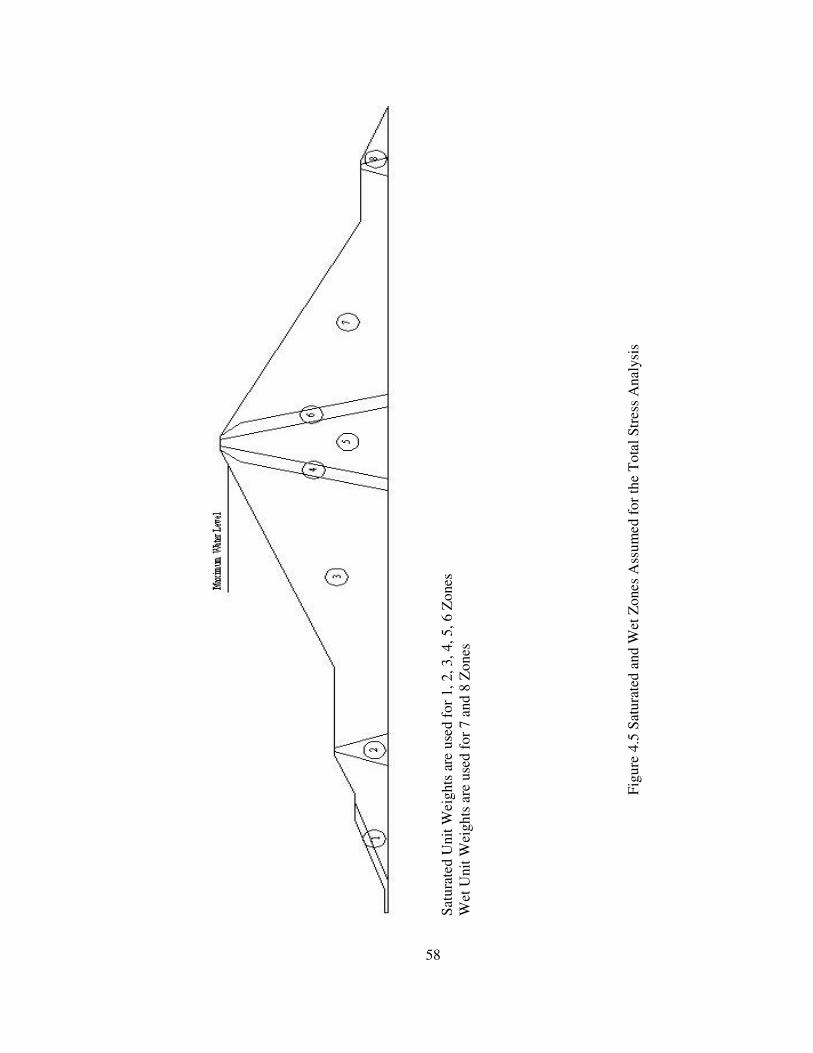
58
Satu
rate
d U
nit W
eigh
ts a
re u
sed
for 1
, 2, 3
, 4, 5
, 6 Z
ones
W
et U
nit W
eigh
ts a
re u
sed
for 7
and
8 Z
ones
Figu
re 4
.5 S
atur
ated
and
Wet
Zon
es A
ssum
ed fo
r the
Tot
al S
tres
s A
naly
sis

59
(2.97-e)2
Gmax(filter) = 360 σ’m0.5 (kg/cm2) (4.3)
(1+e)
(2.97-e)2
Gmax(rockfill) = 440* σ’m0.55 (kg/cm2) (4.4)
(1+e)
(2.97-e)2
Gmax(clay) = 395 σ’m0.69 (kg/cm2) (4.2)
(1+e)
4.4 Dynamic Material Properties of Akköprü Dam
The behavior of soils subjected to dynamic loading is governed by the
cyclic properties of soil which is mostly known as dynamic soil properties. Hence,
determination of the dynamic material properties is a critical task in the evaluation of
the response of dams under cycling loading. A wide variety of field and laboratory
techniques are available to measure the dynamic material properties at low and high
strains as explained in Section 2.4. For many problems dominated by the wave
propagation effects, only low levels of strain are induced in the soil, for the others
such as those involving the stability of masses of soils large strains are induced in the
soil.
The shear moduli are obtained from the ratio G/Gmax where Gmax is the shear
moduli at low strain levels. The maximum shear modulus values for clay, filter, and
rockfill can be calculated by using the following empirical relationships:
where σ’m is the mean effective stress σ’m = (σ’1 + σ’2 + σ’3)/3 and e is the void
ratio. The equation for filter material is suggested by Richart(1970). Other two
equations for clay core and rockfill are suggested by Baba(1982). The void ratio
values are taken from Table 4.3.

60
Table 4.3 Average Void Raito and Poisson’s Ratio of Construction Materials
Material Average Void Ratio Poisson’s Ratio
Clay (CL) 0.41 0.42
Filter 0.47 0.38
Rockfill 0.42 0.30
The finite element program TELDYN requires curves for the variation of
the shear modulus and damping curves with cyclic shear strain (10-4, 10-3, 10-2, 10-1,
1, 10 in percent). The values for the clay core were obtained from Vucetic and Dobry
(1991) and the values for the filter material were obtained from Seed and Idriss
(1984) as shown in Figure 4.6. The curves for rockfill material are defined below
with the Equation 4.5 and 4.6 respectively and the corresponding curves are
illustrated in Figure 4.7.
where γ is the cyclic shear strain.
1.56 x 10⁻³
G/Gmax(rock) = (4.5) 1.56 x 10⁻³ +γ
γ µ(rock) = 0.23 + 0.05 (4.6) 1.56 x 10⁻³ +γ

61
Modulus Degredation Curves
0
0,2
0,4
0,6
0,8
1
1,2
0,0001 0,001 0,01 0,1 1 10
Cyclic Shear Strain (%)
G/G
max Filter
Clay
Figure 4.6 Shear Modulus and Damping Curves for Clay (Vucetic & Dobry, 1991)
and Filter Material (Seed et al., 1984)
Damping Curves
0
5
10
15
20
25
30
35
0,0001 0,001 0,01 0,1 1 10
Cyclic Shear Strain (%)
Dam
ping
Rat
io (%
)
FilterClay

62
Figure 4.7 Shear Modulus and Damping Curves for Rockfill Material (Baba, 1982)
Modulus Degradation Curve
0
0,2
0,4
0,6
0,8
1
1,2
0,0001 0,001 0,01 0,1 1 10
Cyclic Shear Strain (%)
G/G
max
Rockfill
Damping Curve
0
5
10
15
20
25
30
0,0001 0,001 0,01 0,1 1 10
Cyclic Shear Strain (%)
Dam
ping
Rat
io (%
)
Rockfill

63
4.5 Determination of Input Ground Motions to be Used in the Dynamic Analysis
Due to the computational difficulties to handle the alluvium layer in the
finite element mesh in program TELDYN, designed ground motions assessed in
Chapter 3 are carried from the bedrock outcrop to the base of dam body by using the
computer program SHAKE91. In this program, the soil profile is idealized as system
of homogeneous, viscoelastic sublayers of infinite horizontal extent and the response
of the system is calculated considering vertically propagating shear waves. An
equivalent linear procedure is used to account for the nonlinearity of the soil using an
iterative procedure to obtain values for modulus and damping that are compatible
with the equivalent uniform strain induced in each sublayer. Starting with the
maximum shear modulus for each sublayer and a low value of damping, strain
compatible properties are obtained in 5 to 8 iterations for most soil profiles. In this
study, the soil profile of the alluvium layer divided into 10 sublayers and the shear
wave velocities were estimated for each sublayer as shown in Figure 4.8. More
detailed information regarding SHAKE91 is given in Appendix B.
Consequently, using SHAKE91, the input ground motions were assessed at
the base of the dam body. The calculated response spectra for the input ground
motions at the base of the dam are illustrated in Figure 4.9. A comparison of Figure
4.9 with Figure 3.11 shows that the predominant period of the ground motion
remains constant and the peak ground acceleration increases and at the base of the
dam.
Figure 4.8 Shear Wave Velocity Profile of Alluvium Layer

64
Figure 4.9 Acceleration Response Spectra at the Base of Dam Body
Synthetic Record 1
0
0,3
0,6
0,9
0,0 0,5 1,0 1,5 2,0 2,5 3,0 3,5 4,0 4,5 5,0
Period (seconds)
S(a
)g
Montenegro (Yugoslavia)
0
0,3
0,6
0,9
1,2
0,0 0,5 1,0 1,5 2,0 2,5 3,0 3,5 4,0 4,5 5,0
Period (seconds)
S(a
)g
Synthetic Record 2
0
0,3
0,6
0,9
1,2
0,0 0,5 1,0 1,5 2,0 2,5 3,0 3,5 4,0 4,5 5,0
Period (seconds)
S(a
)g
Compano (Italy)
00,30,60,91,21,5
0,0 0,5 1,0 1,5 2,0 2,5 3,0 3,5 4,0 4,5 5,0
Period (seconds)
S(a
)g

65
4.6 Dynamic Analysis of Akköprü Dam
As mentioned before, the plane strain finite element program TELDYN
(Pyke, 1984) was used in the analysis of Akköprü Dam under earthquake shaking.
This program is specifically designed for the analysis of response of soils to
vertically propagating motions caused by ground motions. Moreover, the program
employs equivalent linear method which involves an iterative computation in order
to obtain shear moduli and damping ratios in each element that are compatible with
the average level of shear strain induced by shaking. More detailed information
regarding the program TELDYN is given in Appendix C.
In the dynamic analysis of Akköprü Dam, the dam embankment was
idealized as a two dimensional mesh which was prepared for static analysis prior to
dynamic analyses. The largest cross section of the embankment was subdivided into
quadrilateral and triangular elements as shown in Figure 4.3. There are 2099 nodes
and 2036 elements in the mesh including three different material zones namely, clay,
filter and rockfill. The maximum element size is determined as 5 m by selecting a
maximum frequency of 10 hertz for the analysis as explained in Section 4.3.
The soil properties that influence wave propagation, shear modulus,
damping ratio, poisson’s ratio and density, are used to identify the construction
materials of the dam embankment (Kramer 1996). As known, shear modulus and
damping ratio values are varying with the cyclic shear strain. In order to represent
this nonlinear behavior of the construction material equivalent linear method is
applied in the analysis. The equivalencing process of the program involves the
following two steps:
1) In the first step, shear moduli and damping values are evaluated for each
element that are compatible with the cyclic shear strain. Modulus reduction and
damping curves are used for the assessment of strain dependent dynamic parameters,
which as explained in Section 4.4 before.

66
2) In the second step of the process, the acceleration time history estimated
in Section 4.5 is divided into a number of segments and applied from the base of the
dam body. Thus, the shear stress and shear strain time history in each element are
obtained in time segments similar to the acceleration time history. The program is
then set up to iterate within each segment and to obtain strain compatible values of
the shear modulus and damping ratio. It is necessary to specify initial estimates of
shear modulus and damping ratio to be used in first iteration of the first segment. The
final values computed in the previous segment are used on the first iteration of
subsequent segments. The iteration within each segment ceases when acceptable
convergence is reached. A maximum difference of about 10 % might be considered
to be acceptable. Three to five iterations are normally sufficient to achieve this level
of convergence. The average shear strain used in the determination of the shear
modulus and damping values is taken to be equal to 0.65 times the maximum shear
strain for each segment.
At the end of the analysis fundamental period of the dam, maximum
accelerations and shear stresses at nodal points are obtained. Furthermore, it is
possible to determine the acceleration, shear stress and shear strain time histories for
any node in the model.
4.7 Permanent Displacement Analysis of Akköprü Dam
In this study, permanent displacement of the potential sliding mass obtained
in Section 4.2 was determined by using the Newmark(1965) method. There were 4
different input ground motions applied from the base and each ground motion is
scaled to 0.25g, 0.20g and 0.15g respectively. According to these PGA values
corresponding displacements were calculated in the analysis.
Two computer programs, ACCHIS(Aksar,2000) and PDISP, were used for
the calculation of permanent displacement of the critical slip surface. ACCHIS
calculates the time history of average acceleration for a certain slip surface by using

67
the horizontal nodal accelerations obtained at the end of dynamic finite element
analysis of the dam. The output of ACCHIS was stored in a file and entered to the
program PDISP as an input file. PDISP calculated the corresponding permanent
displacement for the slip surface by double integrating the difference between the
applied and yield accelerations. The codes of the programs are given in Appendix D
and E respectively.

68
CHAPTER V
RESULTS OF THE DYNAMIC ANALYSES OF AKKÖPRÜ DAM
5.1 Seismic Behavior of Akköprü Dam
The fundamental period of Akköprü dam for small strain vibrations can be
estimated from semi-empirical relationship derived by Öner(1984). The equation is
given as follows:
T1=0.0408e-0.555m h0.75 [1+4/(l/h)2]-0.5 (5.1)
where h is the height of the dam in meters, m is an arbitrary index for material
type(m=2 for rockfill dams) and l is the length of the crest in meters. By using
Equation 5.1 with h=112.5 m and l=688.70 m the fundamental period of Akköprü
Dam can be calculated as 0.44 sec. This gives an idea about the fundamental period
of the dam.
In this study, fundamental period of the dam is determined by using the
finite element program TELDYN. The peak ground acceleration of input ground
motion was scaled to 0.01g and the fundamental period was found to be 0.66 sec for
small strain vibrations. As seen from Figure 5.1 the fundamental period of the dam
increases with increasing peak ground acceleration. For 0.20g peak ground
acceleration the period increases to 0.78 sec due to nonlinear behavior of the dam
during stronger shaking. This is somewhat expected because as the intensity of the
ground motion increases, the stiffness of the material decreases and accordingly the
natural period of the dam increases.

69
The maximum acceleration and the acceleration time histories at nodal
points along the vertical centerline of the dam body were obtained from the dynamic
analyses. The nodal points along the vertical centerline of the dam body are shown in
Figure 5.2. The variations of maximum accelerations are plotted for each motion as
illustrated in Figures 5.3. It can be seen from these figures that the distribution of the
maximum acceleration shows a significant increase towards the top part of the dam
body. Furthermore, the acceleration response spectra are determined at four nodal
points (3, 235, 739, 2039), which are located at the crest, two-third of dam height,
one-third of dam height and base of the embankment as shown in Figure 5.4. As
observed in Figure 5.4, predominant period of the earthquake motion remains
constant until one-third of dam height, however after this level it increases.
Moreover, the amplification of the acceleration increases along the dam height.
These findings indicate that the crest of the dam vibrates more severely compared to
the bottom part of the dam as mentioned by Okamoto (1973). Therefore, in the
design process more attention should be given to the crest region.
5.2 Results of Permanent Displacements Analysis
Permanent displacement analyses of Akköprü Dam are carried out for 4
ground motions by using the Newmark’s (1965) procedure. Each ground motion was
scaled to 0.25g, 0.20g and 0.15g respectively. Hence, 12 different displacements
were calculated in the analyses. As an example, the permanent displacement analysis
for the Synthetic Record 1 with 0.20g peak ground acceleration is given in Figure
5.5.
Permanent displacement values for each ground motion were tabulated in
Table 5.1. As seen from the results shown in Table5.1, maximum permanent
displacements are calculated as 34.54 cm, 15.90 cm and 4.80 cm for 0.25g, 0.20g and
0.15g peak ground acceleration values, respectively. The tolerable upper limit for the
permanent displacement of the dam embankments has been arbitrarily suggested as
100 cm by Hyness-Griffin and Franklin (1984). They stated that it could be tolerated
in most dams and in unusual cases, where a dam could not tolerate this displacement

70
due to small freeboard or vulnerability of critical design features to small
displacements, the dam should be reevaluated by other method (Özkan, 1998).
(0,6
6;0,
01)
(0,7
8;0,
2)
0
0,050,1
0,150,2
0,250,3
0,350,4
0,450,5 0,
650,
70,
750,
80,
85
Fund
amen
tal P
erio
d (s
ec)
Peak Ground Acceleration (g)
Figu
re 5
.1 V
aria
tion
of F
unda
men
tal P
erio
d w
ith th
e Pe
ak G
roun
d A
ccel
erat
ion

71
Figu
re 5
.2 L
ocat
ion
of N
odal
Poi
nt N
umbe
rs T
aken
for A
ccel
erat
ion
Res
pons
e Sp
ectra
Out
puts
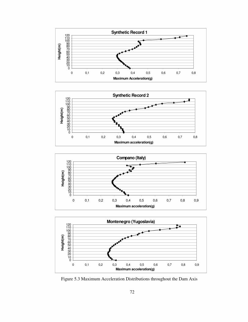
72
Figure 5.3 Maximum Acceleration Distributions throughout the Dam Axis
Synthetic Record 1
0102030405060708090
100110120
0 0,1 0,2 0,3 0,4 0,5 0,6 0,7 0,8
Maximum Acceleration(g)
Hei
ght(
m)
Synthetic Record 2
0102030405060708090
100110120
0 0,1 0,2 0,3 0,4 0,5 0,6 0,7 0,8
Maximum acceleration(g)
Hei
ght(
m)
Compano (Italy)
0102030405060708090
100110120
0 0,1 0,2 0,3 0,4 0,5 0,6 0,7 0,8 0,9
Maximum acceleration(g)
Hei
ght(
m)
Montenegro (Yugoslavia)
0102030405060708090
100110120
0 0,1 0,2 0,3 0,4 0,5 0,6 0,7 0,8 0,9Maximum acceleration(g)
Hei
ght(
m)
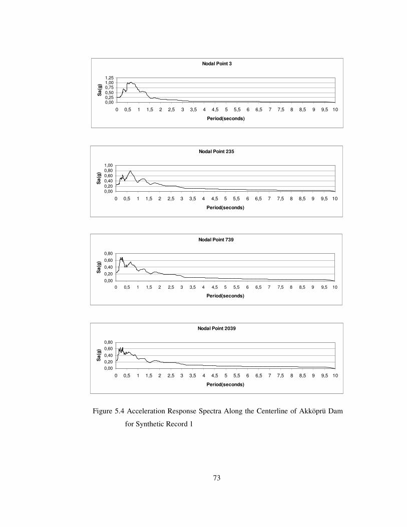
73
Nodal Point 3
0,000,250,500,751,001,25
0 0,5 1 1,5 2 2,5 3 3,5 4 4,5 5 5,5 6 6,5 7 7,5 8 8,5 9 9,5 10
Period(seconds)
Sa(
g)
Nodal Point 235
0,000,200,400,600,801,00
0 0,5 1 1,5 2 2,5 3 3,5 4 4,5 5 5,5 6 6,5 7 7,5 8 8,5 9 9,5 10
Period(seconds)
Sa(
g)
Nodal Point 739
0,000,200,40
0,600,80
0 0,5 1 1,5 2 2,5 3 3,5 4 4,5 5 5,5 6 6,5 7 7,5 8 8,5 9 9,5 10
Period(seconds)
Sa(
g)
Nodal Point 2039
0,000,200,400,600,80
0 0,5 1 1,5 2 2,5 3 3,5 4 4,5 5 5,5 6 6,5 7 7,5 8 8,5 9 9,5 10
Period(seconds)
Sa(
g)
Figure 5.4 Acceleration Response Spectra Along the Centerline of Akköprü Dam
for Synthetic Record 1

74
-0,3
000
-0,2
000
-0,1
000
0,00
00
0,10
00
0,20
00
05
1015
2025
30
Tim
e (s
ec)
Acceleration (m/s2) 0,00
0,03
0,06
0,09
0,12
0,15
0,18
0,21
0,24
0,27
0,30
02
46
810
1214
Tim
e (s
ec)
Velocity (m/s)
0,00
2,00
4,00
6,00
8,00
10,0
012
,00
14,0
016
,00
05
1015
2025
30Ti
me
(sec
)
Displacement (cm)
Figu
re 5
.5 E
xam
ple
of P
erm
anen
t Dis
plac
emen
t Ana
lysi
s (S
ynth
etic
Rec
ord
1 w
ith 0
.02
PGA
)

75
Table 5.1 Results of the Permanent Displacement Analyses
Permanent Displacements (cm)
PGA Synthetic
Record 1
Synthetic
Record 2
Montenegro
(Yugoslavia)
Compano
(Italy)
0.25g 31.44 33.42 34.54 29.18
0.20g 13.45 15.10 15.90 12.57
0.15g 3.80 4.50 4.80 3.34
There is not a definite case in the literature regarding the tolerable damage
of a rockfill dam occurring due to an earthquake event. Omachi and Kuwano (1994)
listed some examples of rockfill dams suffering the strong ground motions. In April
1984, 37 m high rockfill dam suffered some cracks having 30 to 40 cm width, after
an earthquake of M=6.2. In another case, in September 1985 after the earthquake
with M=8.1, La Villita 60 m high rockfill Dam, Mexico, suffered cracks on the crest
and the settlement is estimated as 40 cm in the rockfill zone. Furthermore, the 57 m
high rockfill Sürgü Dam, Turkey, was subjected to longitudinal cracks on the dam
crest and simultaneous settlement on the upstream part of the dam during the 5 May
1986 Malatya Earthquake of M=5.8. The maximum crack width on the dam crest
was 20 cm and upstream part of the crest settled about 15 cm (Özkan,1998).
In this study, for the conservative case, an earthquake having a magnitude of
M=7 and a peak ground acceleration 0.20g, the permanent displacement of the
sliding block on the upstream part of the dam is calculated as 15.90 cm. Considering
the events mentioned above and the suggestion of Hyness-Griffin and
Franklin(1984), it can be said that the dam can stand this amount of displacement.
Figure 5.6 depicts the variation of permanent displacements of Akköprü
Dam with peak ground accelerations. As can be seen from this figure, the rate
increase in the amount of displacement is greater than the increase in the amount of
peak ground acceleration.

76
0510152025303540
0,1
0,15
0,2
0,25
0,3
Pea
k G
roun
d A
ccel
erat
ion(
g)
Permanent Displacement(cm)
Syn
.Rec
ord1
Syn
.Rec
ord2
Mon
tene
gro
Com
pano
Figu
re 5
.6 V
aria
tion
of P
erm
anen
t Dis
plac
emen
t with
the
Peak
Gro
und
Acc
eler
atio
n

77
CHAPTER VI
CONCLUSIONS
For many years, the standard method of evaluating the safety of
embankment dams against sliding during earthquakes has been the pseudostatic
method of analysis. In this method, the dynamic effect of the earthquake is replaced
by an inertial static force acting permanently on the potential sliding mass and the
stability of this sliding mass is represented by a factor of safety of unity or more.
Since pseudostatic is a very simple and straightforward method, many of the dams
designed by using this method as in the case of Akköprü Dam, nevertheless this
method gives no idea about the anticipated displacements.
Finite element method is one of the most powerful technique to evaluate the
stability and behavior of embankment dams under earthquake loading. By
considering the nonlinear behavior of the construction material under earthquake
loading, acceleration, stress-strain time histories and displacements can be calculated
at any point throughout the dam body. The utility of the finite element method has to
be considered with respect to the determination of the correct representative values
of dynamic soil properties, which vary with cyclic shear strain during an earthquake.
Estimation of the ground motion for the dynamic analyses of the
embankment dam requires the determination of proper ground motion parameters
namely duration, predominant period and the peak ground acceleration. In this study,
different values of peak ground acceleration were used to observe its effects on the
behavior of the embankment dam.

78
According to the results obtained from the dynamic analyses of Akköprü
Dam and some other results in the literature, the maximum ground acceleration
increases significantly at the upper part of the dam and reaches to its maximum value
at the crest. Thus, due to greater acceleration at the upper part of the dam, crest
region is more susceptible to seismic excitations. Therefore, the potential sliding
surface is generally observed at the upper part of the dam and cracks usually develop
near the crest after the earthquake.
Acceleration time histories obtained in the finite element analysis can be
used for the calculation of permanent displacement. If the dam embankment or
foundation is not subjected to liquefaction, Newmark’s analysis can be employed to
find the permanent displacement occurring in the potential of sliding mass. Even
though there is not a well defined upper limit for the displacements of the potential
sliding mass, in most dams, a value of 100cm displacement which is suggested by
Hynes- Griffin and Franklin, can be used to evaluate the results of the Newmark’s
analysis.
The most critical task in the dynamic response analysis of the embankment
dams is the assessment of the dynamic properties of the filling material. The
properties of the soils under dynamic loading conditions are nonlinear. During the
earthquake, the stiffness of the soil and the earthquake energy dissipation within the
soil are represented by shear modulus reduction and damping ratio curves
respectively. As the intensity of earthquake motion increases, the stiffness of the soil
decreases and accordingly damping ratio and natural period of the embankment dam
increases.
The amount of maximum permanent displacement of Akköprü Dam is
calculated as 15.90 cm for an earthquake having a magnitude of 7 and a peak ground
acceleration of 0.20g. Considering the tolerable limit of 100 cm estimated by
Hyness–Griffin and Franklin, it is concluded that the Akköprü Dam can stand such
amount of displacement, safely.

79
The change in the amount of permanent displacement is evaluated for
different values of peak ground acceleration. Maximum expected permanent
displacements of the potential sliding mass are obtained as 34.54 cm, 15.90 cm and
5.80 cm for 0.25g, 0.20g and 0.15g peak ground accelerations, respectively. From the
results, it can be observed that the rate increase in the amount of permanent
displacement is greater than the increase of the peak ground acceleration. Thus, it can
be concluded that estimation of the peak ground acceleration in the design process is
very important for determining the displacements obtained by the Newmark’s
method.

80
REFERENCES
Abdel-Gaffar, Ahmed M., Scott, Rnald F., 1979. “Shear Moduli and Damping
Factors of Earth Dam”, Journal of Geotechnical Engineering Division,
ASCE, Vol. 105, No. GT12, pp. 1405-1426.
Aksar, Ü.D., 2001. “A Study on Response of Güldürcek Dam During 6, June, 2000
Çankırı Earthquake” M.S. Thesis, Middle East Technical University,
Ankara.
Ambraseys, N., Smit, P. Berardi, R., Rinaldis, D., Cotton, F. and Berge-Thierry C.,
2000. “European Strong Motion Database”, European Council,
Environmental and Climate Research Program.
Arias, A., 1970. “A Measure of Earthquake Intensity”, in R.J. Hansen, ed. Seismic
Design for Nuclear Power Plants, MIT Press, Cambridge, Massachusetts,
pp. 438-483.
Bakır, S., 1987. “Behaviour of Embankment Dams Under Earthquake Loading and A
Case Study on Sürgü Dam”, M.S. Thesis, Middle East Technical
University, Ankara.
Bilgi, V., 1990. “Toprak ve Kaya Dolgu Barajların Projelendirme Kriterleri”, The
General Directorate of State Hydraulic Works, Ankara.
Bolt, B. A., 1969. “Duration of Strong Motion”, Proceedings of the 4th World
Conference on Earthquake Engineering, Santiago, Chile, pp. 1304-1315.
81
Boore, D.M., 1983. “Stochastic Simulation of High-Frequency Ground Motions
based on Seismological Models of the Radiated Spectra”, Bulletin of the
Seismological Society of America, Vol. 73, pp. 1865-1884
Boore, D.M., Joyner, W.B., and Fumal, T. E., 1993. “Estimation of Response Spectra
and Peak Accelerations from Western North American Earthquakes: An
Interim Report”, U.S. Geological Survey, OFR 93-509.
Boore, D.M., Joyner, W.B., and Fumal, T. E., 1997. “Equations for Estimating
Horizontal Response Spectra and Peak Acceleration from Western north
American Earthquakes: A summary of Recent Work”, Seismological
Research Letters, Vol. 68, No. 1, pp. 128-153.
Borin, D.L., 1983. “SLOPE, Slope Stability Analysis Program”, Geosolve.
Chang, F. K., and Krinitzsky, E. L., 1977. “Duration, Spectral Content and
Predominant Period of Strong Motion Earthquake Records from Western
United States”, Miscellaneous Paper 5-73-1, U.S. Army Corps of Engineers
Waterways Experiment Station, Vicksburg, Mississippi.
Charney, F.A., 1995. “NONLIN Version 5.30, Nonlinear Dynamic Time History
Analysis of Single Degree of Freedom Systems”, Advanced Structural
Concepts, Inc.
Chopra, A.K., 1966. “Earthquake Effects on Dams”, Ph. D. dissertation, University
of California, Berkeley.
De Alba, P.A., Seed, H.B., Retamal, E., Seed, R.B., 1988. “Analyses of Dam
Failures in 1985 Chilean Earthquake”, Journal of Geotechnical Engineering
Division, ASCE, Vol. 114, No. 12, pp. 1415 - 1435.

82
Demirta�, R., 2003. Private Conversation, The General Directorate of Disaster
Affairs, Ankara.
Elgamal, A.-W.M., Scott, R.F., Succarieh, M.F., and Yan, L., 1990. “La Villita Dam
Response During Five Earthquakes Including Permanent Deformation”,
Journal of Geotechnical Engineering Division, ASCE, Vol. 116, No. 10,
pp.1443-1463.
Erdik, M., 1992. “XS, Artificial Earthquake Data Generating Program”, Bo�aziçi
Üniversitesi Kandilli Rasathanesi.
Esteva, L., 1970. “Seismic Risk and Seismic Design Decisions” in R.J. Hansen, ed.,
Seismic Design of Nuclear Power Plants, MIT Press, Cambridge,
Massachusetts.
Hardin, B.O., and Drnevich, V.P., 1972. “Shear Modulus and Damping in
Soils:Design Equations and Curves”, Journal of Soil Mechanics and
Foundations Divisions, ASCE, Vol.98, No. SM7, pp. 667-692
Hyness-Griffin, M.E., Franklin, A.G., 1984. “Rationalizing the Seismic Coefficient
Method”, Miscellaneous Paper GL-84-13, US Army Corps of Engineers,
Washington, DC 20314.
Idriss, I.M., Lysmer, J., Hwang, R.N., and Seed, H.B., 1973. “QUAD-4: A Computer
Program for Evaluating the Seismic Response of Soil Structures by
Variable Damping Finite Element Procedures”, Report No. EERC 73-16,
Earthquake Engineering Research Center, University of California,
Berkeley.
Idriss, I.M., 1991. “Selection of Earthquake Ground Motions at Rock Sites”, Report
Prepared for the Structures Div., Building and Fire Research Lab., NIST.

83
Idriss, I.M. and Sun, J.I. 1992. “SHAKE91, A Computer Program for Conducting
Equivalent Linear Seismic Response Analyses of Horizontally Layered Soil
Deposits”, User’s Guide, University of California, Davis, 13pp.
Ishibashi, I., 1992. Discussion to “Effect of Soil Plasticity on Cyclic Response”, by
M. Vucetic and R. Dobry, Journal of Geotechnical Engineering, ASCE,
Vol. 118, No. 5, pp. 830-832.
Kalkan, E., 2001. “.Attenuation Relationships Based on Strong Motion Data
Recorded in Turkey”, M.S. Thesis, Middle East Technical University,
Ankara, Turkey.
Kramer, S., 1996. Geotecnical Earthquake Engineering, Prentice Hall, Upper Saddle
River, New Jersey.
Lemos, L.J.L., and Coelho, P.A.L.F. 1991. “Displacements of Slopes under
Earthquake Loading”, Proceedings, 2nd International Conference on Recent
Advances in Geotechnical Earthquake Engineering and Soil Dynamics, St.
Louis, Missouri, Vol. 2, pp. 1051-1056.
Lysmer, J., Udaka, T., Seed, H.B., and Hwang, R.N., 1974. “LUSH: A Computer
Program for Complex Response Analysis of Soil-Structure Systems”,
Report No. EERC 74-4, Earthquake Engineering Research Center,
University of California, Berkeley.
Lysmer, J., Udaka, T., Tsai, C.F. and Seed, H.B., 1975. “FLUSH: A Computer
Program for Approximate 3-D Analysis of Soil-Structure Interaction
Problems”, Report No. EERC 75-30, Earthquake Engineering Research
Center, University of California, Berkeley.
84
Makdisi, F.I., Seed, H.B., 1978. “Simplified Procedure for Estimating Dam and
Embankment Earthquake-Induced Deformations”, Journal of Geotechnical
Engineering Division, ASCE, Vol. 104, GT7, pp. 849-867.
Marcuson, W. F., 1981. “Moderator’s report for session on Earth Dams and Stability
of Slopes under Dynamic Loads”, Proceedings, International Conference on
Recent Advances in Geotechnical Earthquake Engineering and Soil
Dynamics, St. Louis, Missouri, Vol. 3, p. 1175.
McCann, M.W., and Shah, H.C., 1979. “Determining Strong Motion Durations of
Earthquakes”, Bulletin of the Seismological Society of America, Vol. 69,
No. 4, pp. 1253-1265.
Newmark, N.M., 1965. “Effects of Earthquakes on Dams and Embankments”,
Geotechnique, Vol.5, No.2.
Okamoto, A., 1973. Introduction to Earthquake Engineering, University of Tokyo
Press.
Öner, M., Yılmaz, Ç., Erdik, M. and Ertu�rul, M.E., 1979. “Earthquake Analyses for
Atatürk Dam Embankment”, METU/EERI Report No. 79-07.
Özkan, M.Y., 1998. “Review of Considerations on Seismic Safety of Embankment
and Earth and Rock-Fill Dams”, Soil Dynamics and Earthquake
Engineering, Vol. 17, pp. 439-458.
Priscu, R., Popovici, A., Stermatiu, D., Stere, C., 1985. Earthquake Engineering for
Large Dams, Editura Acedemici and John Wiley & Sons, Ltd., Romania.
Pyke, R., 1984. “TELDYN, A Computer Program for Plane Strain, Dynamic Finite
Element Analyses of Soils and Simple Structures, Users Manual”, TAGA,
Engineering Software Services.

85
Richart, F. E., Hall, J.R., and Woods, R.D., 1970. Vibration of Soils and
Foundations, Prentice Hall, New Jersey.
Seed H.B., and Idriss, I.M., 1969. “Influence of Soil Conditions on Ground Motions
During Earthquakes”, Journal of Soil Mechanics and Foundations Division,
ASCE, Vol. 95, No. SM1, pp. 99-137
Seed H.B., Lee, K.L., and Idriss, I.M. 1969. “Analysis of Sheffield Dam Failure”,
Journal of Soil Mechanics and Foundations Divisions, ASCE, Vol.95, No.
SM6, pp. 1453-1490.
Seed H.B., and Idriss, I.M., 1970. “Soil Moduli and Damping Factors for Dynamic
Response Analysis”, Report No. EERC 70-10, Earthquake Engineering
Research Center, University of California, Berkeley, California.
Seed, H.B., Makdisi, F.I., and DeAlba, P., 1978. “Performance of Earth Dams
During Earthquakes”, Journal of Geotechnical Engineering Division,
ASCE, Vol. 104, No GT7, Proceedings Paper 13870.
Seed, H.B., 1979. “Considerations in the Earthquake-Resistant Design of Earth and
Rockfill Dams” Geotechnique, Vol.29, No.3, pp. 215-263.
Seed, H.B., Idriss, I.M., Lee, K.L., Makdisi, F.I., 1975. “Dynamic Analysis of the
Slide in the Lower San Fernando Dam During the Earthquake of February
9,1971”, Journal of Geotechnical Engineering Division, ASCE, Vol. 114,
No. 12, pp. 1415 - 1435.
Seed, H.B., Wong, R.T., Idriss, I.M., and Tokimatsu, K., 1984. “Moduli and
Damping Factors for Dynamic Analyses of Cohesionless Soils”, Journal of
Geotechnical Engineering, ASCE, Vol.112, No.11, pp. 1016-1032
86
�ekercio�lu, E., Özgüler, E., 1999. “Geotechnical Investigations on Leakage
Problem of Akköprü Dam, Turkey”, International Commission on Large
Dams, Antalya.
Singh, B., Varshney, R.S., Verghese, B.G., Goel, M.C. and Singh R.P., 1995.
Engineering for Embankment Dams, A.A. Balkema, Rotterdam,
Brookfield.
Sherard, J.L., 1967. “Earthquake Considerations in Earth Dam Design”, Journal of
the Soil Mechanics and Foundations Divisions, ASCE, Vol. 93, No. SM4,
pp. 377-401,
State Hydraulic Works, 1982. “Dalaman, Akköprü, Gökyar, Narlı, Sandalcık ve
Be�konak Baraj Yerleri Deprem Risk Analiz Raporu”, Ministry of Power
and Natural Resources, Ankara, Turkey.
Terzaghi, K., 1950. Mechanism of Landslides, The Geological Survey of America,
Engineering Geology (Berkey) Volume.
Tika-Vassilikos, T.E., Sarma, S.K., and Ambraseys, N., 1993. “Seismic
Displacements on Shear Surfaces in Cohesive Soils”, Earthquake
Engineering and Structural Dynamics, Vol. 22, pp. 709-721.
Trifunac, M.D., and Brady, A.G., 1975b. “A Study of the Duration of Strong
Earthquake Ground Motion”, Bulletin of the Seismological Society of
America, Vol. 61, pp. 581-626.
Tunçer, M., 1995. “Earthquake Behaviour and Permanent Displacement Analysis of
Sürgü Dam: A Reevaluation”, M.S. Thesis, Middle East Technical
University, Ankara, Turkey.

87
Vucetic, M., and Dobry, R., 1991. “Effect of Soil Plasticity on Cyclic Response”,
Journal of Geotechnical ;Engineering, ASCE, Vol.117, No. 1, pp. 89-107.
Wilson, E.L., and Habibullah, A., 1992. SAP90-A Series of Computer Programs for
the Finite Element Analysis of Structures-Structural Analyses Users
Manual”, Computers and Structures, Inc., Berkeley, California.

88
APPENDIX A
EARTHQUAKES WITH M≥≥≥≥4 OCCURRED
DURING THE PERIOD 1900-2002
Here the epicenter map of the earthquakes with magnitudes greater than 4.0
and a list of the earthquakes with their occurring dates, epicenter locations, focal
depths and magnitudes are given.

89
Figure A.1 Earthquakes with M≥4 Occur in Southwestern Anatolia During the Period 1900-2002
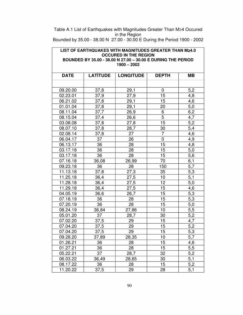
90
Table A.1 List of Earthquakes with Magnitudes Greater Than M≥4 Occured in the Region
Bounded by 35.00 - 38.00 N 27.00 - 30.00 E During the Period 1900 - 2002
LIST OF EARTHQUAKES WITH MAGNITUDES GREATER THAN M≥≥≥≥4.0 OCCURED IN THE REGION
BOUNDED BY 35.00 - 38.00 N 27.00 – 30.00 E DURING THE PERIOD 1900 – 2002
DATE LAT�TUDE LONGITUDE DEPTH MB
09.20.00 37,8 29,1 0 5,2 02.23.01 37,9 27,9 15 4,8 06.21.02 37,8 29,1 15 4,6 01.01.04 37,8 29,1 20 5,0 08.11.04 37,7 26,9 6 6,2 08.15.04 37,4 26,6 5 4,7 03.08.08 37,8 27,8 15 5,2 08.07.10 37,8 28,7 30 5,4 02.08.14 37,8 27 7 4,6 06.04.17 37 26 0 4,9 06.13.17 36 28 15 4,8 03.17.18 36 28 15 5,0 03.17.18 36 28 15 5,6 07.16.18 36,08 26,99 70 6,1 09.23.18 36 28 150 5,7 11.13.18 37,8 27,3 35 5,3 11.25.18 36,4 27,5 10 5,1 11.28.18 36,4 27,5 12 5,0 11.29.18 36,4 27,5 15 4,6 04.05.19 36,6 26,7 15 5,3 07.18.19 36 28 15 5,3 07.20.19 36 28 15 5,0 08.24.19 36,84 27,86 10 5,5 05.01.20 37 28,7 30 5,2 07.02.20 37,5 29 15 4,7 07.04.20 37,5 29 15 5,2 07.04.20 37,5 29 15 5,3 09.28.20 37,89 28,35 10 5,7 01.26.21 36 28 15 4,6 01.27.21 36 28 15 5,5 05.22.21 37 28,7 32 5,2 06.03.22 36,49 28,65 30 5,1 08.17.22 36 28 15 5,2 11.20.22 37,5 29 28 5,1

91
12.06.22 37,5 29 15 5,3 11.27.23 36 26 15 5,0 03.17.25 37,2 26,2 15 5,2 07.29.25 37,5 27,5 15 4,7 02.08.26 37,1 27,9 7 5,3 02.18.26 36,7 27,2 5 4,9 03.16.26 37,5 29 15 6,2 03.18.26 36 29 12 4,9 03.19.26 36 29 15 4,7 03.21.26 36 29 15 5,2 03.28.26 36 29 15 5,0 03.31.26 36 29 15 5,1 04.01.26 36 29 14 5,2 04.20.26 36 29 15 5,0 05.02.26 36 26 15 4,7 05.22.26 36 26 15 5,0 06.06.26 36 26 15 4,7 06.26.26 36,75 26,98 10 7,4 06.26.26 36,5 27,5 15 5,4 06.27.26 36,7 27,76 10 5,4 07.05.26 36,52 26,69 140 6,2 12.07.26 36 27 15 5,1 12.08.26 36 27 15 5,2 12.12.26 36 27 15 4,7 05.20.27 37,5 27,5 15 4,7 04.10.28 37,4 26,1 15 5,0 03.27.29 36,63 26,68 106 5,2 03.27.29 36,4 26,54 80 6,2 11.11.29 36,68 26,21 15 5,7 08.22.30 36,2 27,5 120 5,6 08.09.32 36,71 27,73 110 5,3 12.07.32 36,71 27,33 60 5,2 04.23.33 36,77 27,29 30 6,3 05.15.33 36,35 26,8 10 5,1 07.24.33 37,8 29 15 4,7 08.17.33 37,36 28,82 60 4,7 04.28.36 36,43 27,05 160 5,6 05.01.38 37,2 28,4 15 4,7 03.13.39 36 29 15 5,2 07.24.39 37,2 28,3 15 5,0 05.23.41 37,07 28,21 40 6,0 05.23.41 37,2 28,4 10 4,7 05.23.41 37,13 28,38 40 5,4 05.23.41 37,22 28,35 48 5,3 06.07.41 37,2 28,3 5 4,7 06.23.41 37,2 28,3 7 5,1

92
07.13.41 37,66 26,09 60 5,9 09.21.41 37,5 28,29 70 5,3 10.14.41 37,2 28,4 15 4,8 12.13.41 37,13 28,06 30 6,4 06.21.42 36,12 27,2 40 6,3 01.11.43 37 27,4 19 5,3 10.16.43 36,45 27,94 120 6,5 11.15.43 36,81 28,84 83 5,3 11.20.43 36,44 28,44 40 5,7 01.05.44 36,4 27,4 150 5,7 01.05.44 36,42 27,67 70 5,7 01.08.44 36,8 27,7 15 4,7 03.25.44 37,8 26,8 8 4,7 05.27.44 36,23 27,25 40 6,2 12.21.45 37,9 29 4 4,9 04.12.46 36,24 26,69 80 5,6 01.13.51 36 26 0 4,8 11.05.51 36 29 0 5,3 04.09.52 37,8 26,9 10 4,7 06.09.52 36,83 27,64 20 5,0 09.15.52 37,6 27,6 32 4,8 10.22.52 36,86 27,09 107 5,3 01.12.53 36 28 0 5,0 03.20.53 36,48 28,51 160 4,6 04.17.53 37,6 27,6 16 4,7 06.13.53 36 26,92 40 4,7 12.05.53 36,5 26,8 15 4,8 01.02.54 36,98 27,12 140 5,4 05.01.54 37,8 27 0 5,0 05.01.54 37,88 27,39 30 5,2 05.01.54 37,77 27,12 40 5,3 05.01.54 37,75 27,29 60 5,0 06.17.54 36,52 27,73 60 4,7 08.20.54 37,5 27 15 4,7 09.04.54 36,63 27,1 160 5,7 05.31.55 36 26 15 4,9 07.16.55 37,65 27,26 40 6,6 07.18.55 37,9 27,1 33 4,5 08.28.55 37,4 27,16 20 5,3 11.10.55 37,44 27,23 10 4,7 11.11.55 37,54 26,97 10 4,9 11.11.55 37,5 27,2 18 4,5 05.05.56 36,99 28,63 40 4,9 05.05.56 37 28,2 0 4,7 06.27.56 37,8 27,1 26 4,3 07.08.56 36,9 26 15 4,7

93
07.09.56 36,68 26,05 40 4,9 07.09.56 36,46 26 60 4,8 07.09.56 36,54 26,32 40 4,7 07.09.56 36,72 26,12 10 4,7 07.09.56 36,45 26,09 60 5,0 07.10.56 36,69 26,06 20 4,4 07.10.56 36,72 26,52 10 4,8 07.10.56 36,77 26,23 30 5,3 02.05.57 36,37 28,88 60 5,3 02.09.57 36,75 26,44 40 5,2 04.24.57 36,43 28,63 80 6,6 04.25.57 36,42 28,68 80 6,9 04.25.57 36,16 28,73 80 4,4 04.25.57 36,44 28,89 30 4,4 04.25.57 36,12 28,6 10 5,2 04.26.57 36,22 28,87 50 5,9 04.26.57 36,41 28,8 10 4,9 03.04.58 36,34 27,85 120 5,3 04.24.58 36,76 26,55 10 5,0 05.09.58 36,61 27,6 67 5,3 05.23.58 36,5 28 13 4,4 05.27.58 36,8 26,76 160 5,2 06.30.58 36,29 27,32 100 5,4 09.04.58 36,56 26,72 40 5,2 09.04.58 36,4 27,01 140 5,1 09.04.58 37,9 27,6 20 4,6 12.09.58 36,56 28,16 50 4,7 01.06.59 36,85 29,16 20 4,7 01.06.59 36,66 29,11 30 5,0 01.06.59 36,8 29,2 0 4,6 01.07.59 36,71 29,21 40 5,0 01.09.59 36,55 28,99 40 4,5 01.11.59 36,64 29,12 50 4,9 01.11.59 36,6 29,1 0 4,7 01.14.59 36,05 28,99 60 4,5 01.20.59 36,7 28,7 0 5,0 01.26.59 36,83 29,23 70 5,5 01.26.59 36,7 29 0 4,7 04.08.59 36,57 26,8 160 4,9 04.25.59 36,94 28,58 30 5,9 04.25.59 36,92 28,6 40 5,4 04.30.59 36,22 26,68 100 5,0 05.20.59 36,74 26,67 70 5,0 06.09.59 36,81 29,08 20 4,9 06.10.59 36,8 29,15 50 4,7 07.12.59 36,03 26,28 80 5,4

94
11.15.59 36,8 26 80 5,0 12.08.59 36,91 29,07 70 5,2 01.09.60 36,85 29 70 5,1 01.17.60 37,02 29,11 40 4,5 01.19.60 36,9 28,8 0 4,5 01.19.60 36,7 29 60 4,7 01.20.60 36,7 28,8 0 4,6 01.26.60 36,85 29,02 60 5,3 01.26.60 36,89 28,61 30 4,8 01.26.60 36,93 29,03 50 4,6 01.26.60 36,84 28,96 10 4,6 01.27.60 36,6 28,7 5 4,6 01.28.60 36,6 29,1 8 4,4 01.29.60 36,88 29,04 60 4,7 04.08.60 36,2 28,2 0 4,5 04.10.60 37,73 27,8 40 5,0 04.12.60 37,69 27,7 40 4,8 05.02.60 36,95 26,83 20 4,8 05.15.60 37,2 26,7 0 4,7 11.03.60 36,1 26,1 15 4,7 02.23.61 36,75 27,07 80 5,2 02.23.61 36,6 27,2 15 4,9 02.23.61 36,73 27,22 40 5,1 02.27.61 36,56 27 70 5,2 02.27.61 36,59 27,02 60 5,2 03.13.61 36,21 26,43 10 5,0 05.23.61 36,7 28,49 70 6,5 05.25.61 36,72 26,66 60 5,0 06.21.61 37,87 28,77 60 5,5 08.16.61 36 26 0 5,0 04.16.62 36,15 27,23 140 5,5 04.28.62 36,03 26,87 50 6,0 04.28.62 36,09 26,88 50 5,6 02.16.63 36,47 28,01 40 4,7 03.11.63 37,96 29,14 40 5,6 05.23.63 36,01 29,1 80 4,5 07.08.63 36,48 27,88 80 4,9 07.26.63 36,84 28,76 80 5,2 08.21.63 36,3 26,7 15 4,7 09.29.63 36,44 29 60 5,0 03.31.64 36,43 28,78 57 4,8 05.13.64 36,28 28,21 82 4,5 06.08.64 36,26 28,26 62 4,6 07.18.64 36,13 26,01 99 5,0 09.28.64 36,7 29,2 63 4,4 10.13.64 36,94 28,29 76 4,5

95
01.07.65 36,5 26,85 35 5,0 01.09.65 36 27,4 63 4,4 04.09.65 36,8 26,5 33 4,7 04.29.65 37,14 26,89 8 4,7 05.01.65 37,18 26,91 0 4,6 05.07.65 36,74 26,86 162 4,5 06.10.65 36,44 26,64 142 4,7 06.13.65 37,85 29,32 33 5,1 06.17.65 37,6 28,8 33 4,7 06.17.65 37,77 29,36 37 4,7 07.12.65 37,62 29,35 50 4,6 11.08.65 36 27 0 4,2 11.28.65 36,12 27,43 73 5,7 12.02.65 37,61 29,32 38 4,7 12.07.65 36,25 27 0 4,4 12.08.65 37,3 28,5 0 4,5 12.22.65 37,1 28,1 0 4,5 02.08.66 36,23 28,11 79 4,5 03.08.66 36,5 26,6 0 4,3 03.27.66 37 26,9 0 4,2 03.27.66 37 26,9 0 4,2 03.27.66 37 26,9 0 4,4 03.28.66 37 26,9 0 4,2 03.28.66 37 26,9 0 4,2 03.29.66 37 26,9 0 4,3 03.29.66 37 26,9 0 4,4 04.07.66 36,8 26,7 26 4,2 05.04.66 37,74 27,71 37 4,8 05.07.66 37,75 27,79 9 5,0 07.03.66 36,1 26,5 0 4,2 07.17.66 37,05 27,25 0 4,2 08.18.66 36,22 26,35 133 4,4 09.06.66 36,66 26,63 158 4,4 09.10.66 36,53 26,9 146 4,1 10.13.66 36,14 27,83 7 4,5 11.21.66 36,2 29,3 0 4,5 04.04.67 36,68 29,27 24 4,9 05.22.67 36,59 29,35 54 4,6 06.01.67 36,81 29,26 43 5,0 06.02.67 36,89 29,3 0 4,3 06.07.67 37 26,9 0 4,3 06.18.67 36,78 29,32 35 4,9 07.25.67 37,8 28,6 75 4,4 07.25.67 37,9 28,7 101 4,5 08.09.67 36,98 28,4 64 4,8 08.28.67 36,73 26,74 169 4,5

96
09.05.67 36,72 29,33 24 4,5 10.11.67 36,07 27,12 34 4,6 10.26.67 37,22 29,05 46 5,0 11.13.67 37,78 28,83 34 4,6 12.05.67 36,53 26,85 137 4,6 01.13.68 36,3 27,9 71 4,4 02.07.68 36,65 26,74 153 5,0 02.20.68 36,4 26,2 0 4,1 02.20.68 36,15 27,39 64 4,9 03.30.68 36,7 27,7 64 4,3 07.04.68 36,77 29,03 94 4,4 09.05.68 36,3 26,7 1 4,4 10.06.68 36,96 26,38 17 4,7 10.10.68 36,5 29,2 0 4,5 10.27.68 36,2 27,1 0 4,4 10.28.68 36,75 27,75 0 4,2 10.31.68 36,62 27,01 2 5,1 10.31.68 36,5 27,5 0 4,2 10.31.68 36,75 27,5 0 4,2 11.04.68 36,44 26,98 35 4,6 11.11.68 36,61 27,1 33 4,5 11.12.68 36,74 27,11 26 4,7 11.12.68 36,64 27,16 24 4,6 11.12.68 37,6 28,5 0 4,3 11.16.68 36,6 27,18 0 4,1 11.26.68 36,2 27,3 41 4,3 12.04.68 36,34 26,98 43 4,4 12.04.68 36,48 27,03 36 4,4 12.04.68 36,5 27,02 32 4,7 12.04.68 36,67 27,1 0 4,1 12.04.68 36,71 27,2 58 4,1 12.05.68 36,6 26,92 31 5,4 12.05.68 36,4 27,2 0 4,1 12.21.68 36,6 27,07 30 4,5 12.21.68 36,6 27,3 0 4,2 12.21.68 36,56 27,4 30 4,2 01.14.69 36,11 29,19 22 5,6 02.19.69 37,79 28,2 0 4,2 02.26.69 36,66 27,18 33 4,4 03.23.69 37,9 27,6 0 4,9 03.24.69 36,6 28,6 0 4,6 04.21.69 36,22 28,27 11 4,6 04.24.69 36,35 28,73 53 4,7 04.26.69 36,71 28,5 13 4,3 04.27.69 36,54 28,21 33 4,7

97
05.23.69 36,1 27 0 4,3 08.03.69 37 29 57 4,1 09.06.69 36,73 28,35 72 5,0 09.22.69 36,57 28,01 86 4,6 12.21.69 36,66 28,42 69 4,6 01.26.70 37 28,5 0 5,1 02.18.70 36,3 27 0 4,7 02.18.70 36,41 27,12 11 4,6 02.18.70 36,68 27,14 10 4,6 02.20.70 36,4 27,2 33 4,9 02.20.70 36,55 27,26 20 4,6 02.24.70 36,37 27,94 102 4,2 03.01.70 36,9 29,1 0 4,5 03.02.70 36,8 28,8 49 4,6 03.27.70 36,03 28,36 0 4,5 03.28.70 37,2 29 0 4,3 04.17.70 37,09 26,92 32 4,7 04.19.70 36 27,1 0 4,5 04.24.70 36,75 28,66 34 4,6 06.28.70 36,2 27,1 0 4,5 09.28.70 37,09 28,59 24 4,6 10.19.70 37,01 29,01 11 4,6 10.24.70 36,86 28,8 28 4,1 11.21.70 36,88 28,92 19 4,5 12.28.70 37,06 29,02 7 4,4 12.28.70 37,09 28,91 23 4,4 12.29.70 36,03 28,34 26 4,6 12.30.70 36,05 28,34 36 4,2 12.30.70 36,96 28,94 23 5,1 12.31.70 37,11 29 38 4,4 01.02.71 37,07 29,04 7 4,4 01.16.71 36,63 26,9 157 4,2 02.20.71 37,82 29,39 36 4,5 03.18.71 36,32 26,98 141 4,4 09.03.71 36,81 28,79 0 4,6 10.16.71 36,63 28,54 61 4,8 11.12.71 36,61 27,09 23 5,1 01.20.72 36,64 27,15 16 4,6 01.20.72 36,64 27,23 34 4,8 03.25.72 36,67 27,51 55 4,4 03.31.72 36,68 27,36 0 4,1 03.31.72 36,62 27,09 18 4,4 08.29.72 37 29,14 0 4,4 10.23.72 37,78 26,32 28 4,4 12.24.72 36,19 27,77 35 4,3 01.13.73 36,3 26,78 54 4,2

98
09.12.73 36,56 26,99 157 4,3 02.05.74 36,74 26,86 157 4,7 03.12.74 36,76 26,4 45 4,8 05.09.74 36,62 27,22 26 4,4 05.12.74 36,71 26,89 149 4,2 05.16.74 36,11 27,27 32 4,1 07.09.74 36,57 28,48 49 4,9 05.31.75 36,74 28,23 34 4,1 06.02.75 36,47 26,52 31 4,7 09.23.75 36,6 26,76 158 4,6 11.12.75 36,28 28,15 65 5,3 12.08.75 36,43 27,86 5 4,3 01.10.76 36,8 27,92 31 4,6 02.10.76 36,82 27,93 39 4,7 04.06.76 36,62 27,28 151 4,5 05.01.76 36,95 27,94 31 4,3 08.15.76 37,84 28,77 11 5,3 08.17.76 36,74 27,07 160 5,0 08.18.76 36,48 26,95 148 4,3 08.18.76 36,73 27,42 157 4,7 08.19.76 37,71 29 20 5,0 09.12.76 36,59 26,96 154 4,2 12.24.76 36,1 26,77 159 4,3 03.08.77 36,54 28,54 65 4,1 03.28.77 36,82 27,52 36 4,8 07.12.77 36,62 26,97 157 4,4 07.14.77 36,16 27,69 9 4,3 10.27.77 37,87 27,88 16 4,7 01.11.78 37,48 28,86 5 4,9 03.13.78 37,81 26,88 5 4,7 04.03.78 37,22 28,99 0 4,9 06.17.78 37,54 28,81 0 4,8 10.25.78 36,69 27,07 168 4,3 10.29.78 36,04 27,24 9 4,1 11.28.78 36,04 26,39 115 5,0 02.28.79 36,63 27,05 136 4,3 06.22.79 36,8 29,03 11 4,1 08.23.79 37,99 28,91 10 4,2 09.01.79 36,43 26,31 10 4,2 09.03.79 36,05 27,68 89 4,1 10.21.79 36,8 27,77 10 4,4 10.26.79 36,91 27,76 10 4,6 11.06.79 36,83 27,99 10 4,6 11.09.79 36,89 27,93 5 4,4 02.18.80 36,98 27,92 7 4,6 02.19.80 36,95 27,89 4 4,4

99
04.11.80 36,96 27,84 0 4,6 04.15.80 36,68 27,34 0 4,2 04.29.80 37,07 28,73 32 4,4 06.11.80 36,06 27,77 108 4,3 10.04.80 37 28,8 26 5,0 11.11.80 36,9 28,82 0 4,9 11.11.80 36,9 28,75 1 4,1 01.03.81 36,9 28,6 0 4,8 04.27.81 36,05 28,88 37 4,6 05.11.81 36,78 28,08 22 4,7 06.08.81 36,22 28,87 68 4,1 11.16.81 36,64 26,82 161 4,7 11.19.81 36,33 27,72 41 4,3 12.21.81 36,58 26,81 2 4,6 01.09.82 37,92 28,87 3 4,6 01.24.82 36,61 27,52 146 4,5 04.18.82 36,65 27,11 155 5,0 05.04.82 36,44 26,78 10 4,6 05.05.82 36,35 27 0 4,3 05.11.82 36,93 28,86 12 4,2 05.25.82 36,87 27,83 10 4,4 06.07.82 36,98 27,92 10 4,7 06.12.82 36,92 27,89 10 4,3 06.12.82 36,92 27,89 8 4,1 06.12.82 36,89 27,78 10 4,4 06.28.82 37 27,98 1 4,3 06.29.82 37 28,03 10 4,5 08.30.82 36,76 27,21 10 4,3 02.12.83 36,78 27,52 38 4,5 02.28.83 36,3 27,72 107 4,5 03.22.83 37,01 29,24 10 4,4 03.24.83 37,11 29,35 10 4,6 04.14.83 36,57 27,03 10 4,7 04.23.83 36,24 26,43 136 4,4 06.14.83 36,44 28,44 94 4,1 06.25.83 37,79 29,35 10 4,1 08.04.83 37,84 27,59 0 4,7 09.27.83 36,72 26,93 160 5,4 11.18.83 36,87 28,82 15 4,5 11.21.83 36,26 27,1 24 4,5 11.21.83 36,42 26,92 43 4,6 01.31.84 37,03 28 15 4,9 02.05.84 37,21 28,67 30 5,0 02.06.84 37,09 28,15 26 4,9 03.14.84 37,13 27,96 10 4,6 03.21.84 37,79 28,42 33 4,2

100
03.25.84 37,74 28,68 0 4,5 04.21.84 36,06 27,24 49 4,7 04.23.84 37,85 26,87 29 4,6 04.23.84 37,83 26,87 27 4,8 04.26.84 37,22 28,42 9 4,3 05.04.84 37,89 29,24 22 4,7 06.07.84 37,23 28,72 10 4,3 06.20.84 36,69 27,05 166 4,7 07.19.84 36,13 27,3 55 4,5 09.23.84 36,52 26,49 155 4,4 11.15.84 36,3 27,61 5 4,3 11.18.84 37,95 28,95 13 4,1 12.16.84 36,35 26,82 147 4,2 02.16.85 36,52 26,52 142 4,5 02.17.85 36,61 27,67 128 4,7 02.25.85 36,43 26,7 157 4,2 04.10.85 36,77 27,46 5 4,5 04.10.85 36,8 27,54 20 5,0 04.23.85 36,29 26,95 137 4,5 05.20.85 36,16 28,82 51 4,8 06.05.85 36,2 27,9 44 4,3 08.23.85 37,23 28,79 11 4,5 09.11.85 36,43 28,87 58 4,6 11.18.85 36,03 27,42 10 4,2 11.24.85 37,65 27,57 23 4,5 12.03.85 36,64 26,89 156 4,6 12.06.85 36,97 28,85 9 4,6 12.23.85 36,88 26,58 39 4,2 12.23.85 36,81 26,62 25 4,9 02.21.86 36,38 26,52 146 4,8 03.19.86 37,55 26,93 19 4,7 03.19.86 37,61 26,93 5 4,6 05.03.86 36,93 28 119 4,2 07.29.86 36,69 27,94 109 4,1 08.11.86 36,2 26,83 128 4,1 08.17.86 36,53 26,96 154 4,2 10.20.86 37,79 27,38 3 4,5 12.31.86 36,19 27,1 42 4,7 01.06.87 36,19 28,03 7 4,3 01.06.87 36,15 28,12 16 4,4 01.07.87 36,17 28,11 35 4,2 01.31.87 36,16 28,14 17 4,3 02.01.87 36,22 28,02 10 4,1 02.01.87 36,08 28,12 25 4,4 04.04.87 36,92 28,39 20 4,6 04.08.87 36,35 26,05 133 4,1

101
04.08.87 36,09 27,12 46 4,4 04.17.87 36,07 27,13 42 4,3 05.01.87 36,07 27,34 39 4,7 05.02.87 36,03 27,33 24 4,1 05.07.87 36,63 26,75 153 4,7 06.11.87 36,34 26,53 147 4,4 06.19.87 36,8 28,18 85 5,0 07.11.87 36,64 26,9 161 4,5 07.18.87 36,15 28,24 51 4,2 08.31.87 36,58 27,71 113 4,1 09.03.87 36,65 27,17 162 4,2 09.15.87 37,85 26,95 1 4,6 10.05.87 36,24 28,27 27 5,1 10.06.87 36,21 28,29 16 4,6 10.06.87 36,25 28,26 36 4,5 10.06.87 36,28 28,24 20 4,5 10.06.87 36,28 28,33 14 4,7 10.09.87 36,28 28,35 10 4,4 10.09.87 36,24 28,31 8 4,6 10.12.87 36,26 28,3 10 4,6 10.25.87 36,3 28,35 24 4,6 10.25.87 36,28 28,17 8 4,2 10.25.87 36,38 28,21 18 4,5 10.27.87 36,19 28,33 6 4,6 11.26.87 36,06 29,15 14 4,5 12.12.87 36,78 28,28 78 4,3 12.26.87 36,89 27,71 35 4,7 12.30.87 36,88 27,72 30 4,8 01.30.88 36,29 28,22 1 4,5 05.24.88 36,04 28,12 7 4,2 06.02.88 36,28 26,73 130 4,1 08.15.88 37,89 29,24 11 4,7 08.24.88 36,59 26,29 26 5,0 09.11.88 36,26 26,35 124 4,6 09.27.88 36,02 27,16 50 4,2 10.26.88 37,96 27,69 19 4,8 10.29.88 36,1 28,15 4 4,7 12.30.88 36,07 27,27 31 4,5 01.05.89 37,09 27,69 10 4,6 01.08.89 37 27,6 8 4,4 02.19.89 36,98 28,2 1 4,8 02.24.89 37,73 29,33 11 5,0 02.24.89 37,72 29,26 19 4,4 02.24.89 37,73 29,24 23 4,5 03.08.89 36,33 27,74 96 4,5 04.27.89 37,04 28,17 12 5,3

102
04.28.89 37,03 28,11 17 5,1 04.28.89 37,05 28,03 6 4,1 06.24.89 37,02 28,06 21 4,3 07.19.89 36,14 27,19 49 4,3 08.16.89 36,08 28,85 58 4,2 11.01.89 36,47 26,99 142 4,6 11.24.89 36,71 26,61 11 4,6 12.07.89 36,68 26,95 159 4,2 12.18.89 37,87 29,22 7 4,5 12.22.89 36,91 26,42 10 4,6 12.26.89 36,41 26,79 142 4,3 12.31.89 36,14 27,08 10 4,6 01.08.90 36,08 27,15 26 4,3 01.10.90 36,04 27,1 26 4,6 01.13.90 36,1 27,15 28 4,7 01.13.90 36,09 27,16 23 4,7 01.13.90 36,16 27,1 6 4,8 01.13.90 36,12 27,17 1 4,7 01.13.90 36 27,19 12 4,4 01.14.90 36,04 27,14 23 4,6 01.14.90 36,12 27,14 16 4,4 01.14.90 36,13 27,14 13 4,7 01.14.90 36,04 27,12 37 4,1 01.17.90 36,05 27,14 42 4,5 01.25.90 36,07 27,26 22 4,6 01.25.90 36,09 27,27 23 4,6 01.28.90 36,06 27,18 24 4,4 01.28.90 36,09 27,14 10 4,7 02.08.90 36,66 27,07 159 4,6 02.12.90 36,2 27,1 7 5,0 02.19.90 36,1 27,18 20 4,4 02.19.90 36,11 27,18 37 4,7 02.19.90 36,19 27,14 40 4,7 02.20.90 36,16 27,09 20 4,3 02.21.90 36,05 27,21 54 4,4 02.23.90 36,05 27,15 20 4,8 04.14.90 36,1 27,11 35 4,7 04.20.90 36,18 27,13 22 4,7 04.22.90 36,53 26,88 149 4,6 05.07.90 36,27 27,14 10 4,5 05.15.90 36,1 27,18 11 4,5 05.25.90 36,89 28,64 10 4,2 05.26.90 36,85 28,66 12 4,1 06.13.90 36,53 26,98 10 4,8 06.26.90 37,33 29,23 19 4,2 08.28.90 36,27 27,22 41 4,6

103
09.01.90 37,02 27,98 7 4,5 11.23.90 36,35 26,85 131 4,1 01.20.91 36,32 26,4 144 4,1 01.21.91 36,63 26,23 10 4,7 01.25.91 36,98 28,83 2 4,3 06.02.91 36,41 28,47 14 4,2 07.18.91 36,09 27,19 108 4,7 07.30.91 36,32 28,21 48 4,3 04.07.92 36,7 26,35 19 4,8 04.23.92 37,33 28,14 31 4,1 05.15.92 37,71 27,62 4 4,3 06.01.92 36,05 28,3 89 4,2 09.30.92 37,25 29,37 10 4,1 11.06.92 37,84 26,79 10 4,1 11.10.92 37,03 27,85 10 4,7 12.25.92 37,21 28,15 3 4,5 01.14.93 37,2 28,3 22 4,6 01.18.93 37,82 28,5 42 4,3 03.05.93 36,84 27,29 10 4,3 03.05.93 36,43 26,68 148 4,2 04.15.93 36,3 26,61 128 4,5 04.19.93 36,36 27,94 34 4,3 04.24.93 36,46 26,8 157 4,2 08.26.93 36,77 28,05 36 5,2 12.02.93 36,78 26,71 10 4,2 03.28.94 36 28,27 5 4,2 04.03.94 37,22 28,96 5 4,2 11.09.94 36,98 29,06 24 4,2 11.13.94 36,91 29,05 10 4,6 11.13.94 36,91 28,98 26 4,5 11.13.94 37,03 28,94 10 4,9 01.22.95 36,9 29,02 16 4,3 01.25.95 36,22 29,3 51 4,4 02.12.95 36,4 26,86 147 4,1 02.28.95 36,33 29,14 55 4,2 03.07.95 36,76 27,76 13 4,9 07.04.95 36,87 28,06 41 4,1 08.03.95 37,4 27,34 33 4,2 08.22.95 36,61 26,71 167 5,0 09.21.95 36,48 26,79 147 4,7 09.28.95 36,63 29,37 22 4,4 10.30.95 36,33 28 43 4,2 10.30.95 36,51 28,15 18 4,2 11.30.95 36,54 27,11 134 4,8 01.02.96 36,19 27,39 38 4,2 02.03.96 37,51 26,86 11 4,5

104
04.02.96 37,84 26,98 11 5,2 04.04.96 37,89 26,88 12 4,1 04.12.96 36,59 27,04 162 5,2 04.26.96 36,34 27,96 72 5,1 04.29.96 37,06 27,5 1 4,2 04.29.96 37 27,47 10 4,2 04.29.96 37 27,59 10 4,2 05.20.96 37,46 27,55 9 4,2 05.21.96 36,52 26,71 151 4,2 07.20.96 36,13 27,05 27 5,6 07.20.96 36,14 27,16 42 4,3 07.20.96 36,22 27,13 54 4,2 07.20.96 36,17 27,23 54 4,1 07.20.96 36,26 27,15 38 4,6 07.20.96 36,12 27,31 48 4,1 07.20.96 36,17 27,21 17 4,8 07.20.96 36,1 27,17 37 4,3 07.20.96 36,01 27,16 39 4,3 07.21.96 36,11 27,2 5 4,1 07.21.96 36,23 27,15 5 4,2 07.21.96 36,1 27,3 35 4,2 07.21.96 36,13 27,21 32 4,4 07.22.96 36,06 27,19 36 4,1 07.22.96 36,08 27,12 25 4,7 07.22.96 36,38 26,98 31 4,2 07.22.96 36,2 27,28 40 4,2 07.22.96 36,27 27,42 10 4,2 07.22.96 36,36 27,27 5 4,4 07.22.96 36,17 27,18 32 4,1 07.22.96 36,08 27,19 24 4,1 07.22.96 36 27,5 38 4,4 07.22.96 36,26 27,2 25 4,2 07.23.96 36,17 27,3 68 4,3 07.23.96 36,15 27,18 5 4,2 07.23.96 36,65 27,15 36 4,4 07.23.96 36,25 27,29 54 4,2 07.23.96 36,2 27,22 26 4,6 07.24.96 36,63 27,19 17 4,6 07.24.96 36,71 27,17 44 4,2 07.24.96 36,61 27,27 59 4,2 07.24.96 36,22 27,21 37 4,2 07.24.96 36,2 27,2 9 4,2 07.24.96 36,2 27,32 9 4,2 07.24.96 36,68 27,15 25 4,5 07.24.96 36,26 27,08 1 4,2 07.25.96 36,26 27,16 5 4,2

105
07.25.96 36,24 27,24 5 4,2 07.26.96 36,27 27,21 58 4,2 07.26.96 36,27 27,1 8 4,2 07.26.96 36,13 27,15 32 4,3 07.28.96 36,1 27,2 38 4,3 07.28.96 36,36 27,14 1 4,2 07.29.96 36,71 27,13 2 4,2 07.30.96 36,21 27,21 10 4,2 07.30.96 36,25 27,23 5 4,2 07.30.96 36,1 27,28 7 4,2 07.31.96 36,13 27,23 36 4,3 07.31.96 36,14 27,15 5 4,2 07.31.96 36,1 27,04 5 4,2 08.01.96 36,17 27,17 5 4,2 08.01.96 36,29 27,15 5 4,2 08.03.96 36,31 26,83 5 4,2 08.06.96 36,31 27,06 5 4,2 08.08.96 36,19 27,1 5 4,2 08.10.96 36,3 27,09 10 4,2 08.11.96 36,21 27,13 27 4,1 08.14.96 36,28 27,09 5 4,2 08.18.96 36,24 27,22 27 4,4 08.19.96 36,61 27,19 5 4,2 08.19.96 36,6 27,01 5 4,2 08.20.96 36,25 27,24 31 4,1 08.23.96 36,55 27,05 20 4,2 08.31.96 36,39 26,98 5 4,2 08.31.96 36,43 27,02 5 4,2 09.02.96 36,3 27,2 10 4,2 09.10.96 36,25 27,35 6 4,2 09.22.96 36,08 27,14 14 4,2 09.27.96 36,39 27,1 53 4,2 11.03.96 36,21 27,1 24 4,2 11.06.96 36,28 27,1 34 4,4 11.06.96 36,23 27,03 5 4,2 11.06.96 36,26 27,11 42 4,2 11.07.96 36,86 27,62 5 4,2 11.28.96 37,02 26,65 28 4,2 12.10.96 36,79 27,57 27 4,2 12.10.96 37,14 26,88 7 4,2 12.12.96 36,63 26,73 165 4,2 12.15.96 36,62 26,9 161 4,2 06.02.97 36,04 27,14 5 4,2 06.04.97 36,6 26,4 28 4,1 07.27.97 36,18 27,72 5 4,2 08.08.97 36,51 27,11 5 4,3

106
08.21.97 36,45 27,21 17 4,2 08.27.97 36,5 27,12 32 4,4 08.29.97 36,51 27,33 5 4,2 09.25.97 36,31 26,6 162 4,2 10.18.97 36,5 27,22 5 4,2 10.24.97 36,46 26,57 155 4,2 12.27.97 36,56 27,16 17 4,3 02.13.98 36,27 28,45 77 4,8 02.24.98 36,3 28,22 31 4,5 03.10.98 36,04 26,03 143 4,4 07.09.98 37,87 26,79 17 4,9 10.03.98 36,13 28,42 70 4,1 10.17.98 36,67 26,7 159 4,2 10.26.98 36,81 28,97 5 4,1 10.30.98 36,17 27,2 11 4,2 11.01.98 36,34 27,06 5 4,1 11.03.98 36,28 27,15 8 4,1 11.19.98 36,59 27,11 6 4,3 11.25.98 36,64 26,35 9 4,3 12.03.98 36,36 26,76 151 4,1 03.03.99 37,29 27,05 3 4,1 03.29.99 37,14 28,8 38 4,2 04.08.99 36,49 26,68 155 4,2 07.26.99 36,64 27,15 153,7 4,3 08.02.99 36,52 29,17 16 4,4 10.05.99 36,75 28,24 16,7 4,8 10.05.99 36,78 28,13 6,3 4,2 12.26.99 36,55 28,03 89 4,1 02.28.00 36,1 26,52 128 4,4 02.28.00 37,05 27,5 10 4,3 04.21.00 37,7 29,25 6,8 4,9 04.27.00 37,88 29,22 10 4,1 08.10.00 37,26 28,96 29 4,1 09.16.00 36,72 27,5 33 4,5 10.04.00 37,92 29,05 8 4,7 10.04.00 37,95 28,91 5 4,3 10.18.00 36,22 28,69 10 4,4 01.04.01 37,66 26,86 11 4,1 02.18.01 37,98 26,66 6 4,2 03.01.01 37,84 26,81 10 4,1 04.06.01 36,17 26,91 151 4,4 04.09.01 36,43 28,58 79 4,2 06.12.01 37,59 26,84 11 4,2 06.30.01 37,28 26,83 27 4,2 10.08.01 36,74 28,18 88 4,2 07.30.02 37,7 29,16 11 4,6

107
APPENDIX B
DESCRIPTION OF THE COMPUTER PROGRAM TELDYN
TELDYN is a computer program specifically designed for analysis of the
response of soils to vertically propagating motions caused by earthquakes. An
equivalent linear procedure is used to account for the nonlinearity of the soil.
Furthermore, it is possible for the user to divide the input acceleration history into
segments and the shear moduli and the damping ratios are then set to be compatible
with the average shear strains within each segment. An option is also provided in
TELDYN whereby the excess pore pressures in saturated elements can be computed
at the end of each segment and the shear moduli can then be determined in the next
segment as a function of the reduced mean effective stress.
Here the basic steps of input and output of the program are given:
A. Input Data
1) Nodes
2) Elements
3) Boundary Conditions
a) Compliant boundary
b) Viscous boundary
c) Mixed boundary
4) Material Properties
a) Modulus Reduction Curves of Construction Materials
b) Damping Curves of Construction Materials
c) Pore Pressure Generation Curves
d) Specific Values of Material Parameters

108
e) Saturated Elements
5) Input Motion
a) Data about Horizontal Input Motion
b) Data about Vertical Input Motion
B. Output Options
1) Print Options
2) Restart Options

109
APPENDIX C
DESCRIPTION OF THE COMPUTER PROGRAM SHAKE91
The soil profile is idealized as a system of homogeneous, visco-elastic
sublayers of infinite horizontal extent. The response of this system is calculated
considering vertically propagating shear waves. An equivalent linear procedure is
used to account for the nonlinearity of the soil using an iterative procedure to obtain
values for modulus and damping that are compatible with the equivalent uniform
strain induced in each sublayer. Thus, at the outset, a set of properties (shear
modulus, damping and total unit weight) is assigned to each sublayer of the soil
deposit. The analysis is conducted using these properties and the shear strains
induced in each sublayer is calculated. The shear modulus and the damping ratio for
each sublayer are then modified based on the applicable relationship relating these
two properties to shear strain. The analysis is repeated until strain-compatible
modulus and damping values are arrived at. Starting with the maximum shear
modulus for each sublayer and a low value of damping, essentially (ie, difference
less than one percent) strain compatible properties are obtained in 5 to 8 iterations for
most soil profiles.
The following assumptions are incorporated in the analysis:
1) Each sublayer, m, is completely defined by its shear modulus, Gm,
damping ratio, µm, total unit weight, γtm (or corresponding mass density,
ρm) and thickness, hm; these properties are independent of frequency.
2) The responses in the soil profile are caused by the upward propagation
of shear waves from the underlying rock half-space.

110
3) The shear waves are specified as acceleration ordinates at equally
spaced time intervals. (Cyclic repetition of the acceleration time history
is implied in the solution).
4) The strain dependence of the shear modulus and damping in each
sublayer is accounted for by an equivalent linear procedure based on an
equivalent uniform strain computed in that sublayer. The ratio of this
equivalent uniform strain divided by the calculated maximum strain is
specified by the user and is assumed to be the same for all sublayers.
The options incorporated into SHAKE91 are as follows:
1) Dynamic soil properties
2) Data for soil profile
3) Input motion
4) Assignment of object motion to the top of a specified sublayer
5) Number of iterations specified and ratio of uniform strain to maximum
strain
6) Sublayers at top of which peak accelerations and time histories are
computed and saved
7) Sublayer at top of which time history of shear stress or strain is
computed and saved
8) Save time history of object motion
9) Compute response spectrum
10) Compute amplification spectrum
11) Compute Fourier amplitudes

111
APPENDIX D
COMPUTER PROGRAM ACCHIS
In order to determine the time history of average acceleration of the critical
slip surface a computer program called as ACCHIS has been written by using the
FORTRAN programming language.
The input file of the program includes the elements with their nodes and
masses and the acceleration time histories at the nodal points of the sliding surface
which are computed by using the finite element program TELDYN in this study.

112
dimension nelco(4,4),xmass(4),ac(4,2200),avac(4,2200)
*,force(4,2200),forcet(2200),acav(2200)
character*4 a
open(1,file='akkxs1')
open(2,file='akkxs1acc')
read(1,100) nel,acr,dt,nt
print*, nel,acr,dt,nt
do 10 k=1,nel
read(1,150) (nelco(k,i),i=1,4),xmass(k)
print*,(nelco(k,i),i=1,4),xmass(k)
10 continue
j=0
do 20 kk=1,nel
25 rewind 1
j=j+1
do 21 l=1,nt
21 ac(j,l)=0
continue
30 read(1,200) a
if (a.ne.'node') goto 30
backspace 1
read(1,250) nn
if (nn.ne.nelco(kk,j)) goto 30
read(1,300) (ac(j,jj),jj=1,nt)
if (j.lt.4) goto 25
continue
do 35 ii=1,nt
avac(kk,ii)=(ac(1,ii)+ac(2,ii)+ac(3,ii)+ac(4,ii))/4
35 continue
j=0
rewind 1

113
20 continue
do 40 kj=1,nel
do 40 kl=1,nt
force(kj,kl)=avac(kj,kl)*xmass(kj)
40 continue
do 50 km=1,nt
forcet(km)=0
do 50 kn=1,nel
forcet(km)=forcet(km)+force(kn,km)
50 continue
totmass=0
do 55 jk=1,nel
totmass=totmass+xmass(jk)
55 continue
do 60 jl=1,nt
acav(jl)=forcet(jl)/totmass
write(2,350) acav(jl)
60 continue
100 format(i5,2f5.0,i5)
150 format(4i5,f4.2)
200 format(a4)
250 format(4x,i2)
300 format(8f9.4)
350 format(f9.6)
stop
end

114
APPENDIX E
COMPUTER PROGRAM PDISP
In order to calculate the permanent displacement from a given average time
history of the sliding mass, the computer program PDISP is written in MATLAB.
The steps of the program was previously defined in Section 2.5. The input file
obtained from program ACCHIS is AccRecord1 and the output files are vel and disp.
Here the program written for Synthetic Record 1 is given as an example.

115
a=load('AccRecord1.txt');
plot(a);
figure
sum=0;
a=a;
for i=1:2200
if((a(i)<=.24) && (sum<=0))
velocity(i)=0;
t=i;
elseif (a(i)>.24) || (sum>0)
a(i)=a(i)-.24;
y=t+1;
for x=y:i
vel(i)=trapz(a(y:i))*.025;
sum=vel(i);
end
end
end
for k=1:2200
if(vel(k)<0)
vel(k)=0;
end
end
vel=vel;
plot(velocity)
for z=1:2200
disp(z)=trapz(vel(1:z))*.025;
sum=disp(z);
end
figure
plot (disp)