dynamic modelling and optimisation of carbon management ... · 7.3.4 set 3 – optimisation of...
TRANSCRIPT

Dynamic Modelling and Optimisation
of Carbon Management Strategies
in Gold Processing
Pornsawan Jongpaiboonkit
B.E. (Hons), B.Com.
University of Western Australia
This thesis is presented for the degree of
Doctor of Philosophy
School of Engineering
AJ Parker CRC for Hydrometallurgy
Murdoch University
April 2003

ii
I declare that this thesis is my own account of my research and contains as its main
content work, which has not been previously submitted for a degree at any tertiary
education institution.
Pornsawan Jongpaiboonkit
April 2003

iii
Abstract
This thesis presents the development and application of a dynamic model of gold
adsorption onto activated carbon in gold processing. The primary aim of the model is to
investigate different carbon management strategies of the Carbon in Pulp (CIP) process.
This model is based on simple film-diffusion mass transfer and the Freundlich isotherm
to describe the equilibrium between the gold in solution and gold adsorbed onto carbon.
A major limitation in the development of a dynamic model is the availability of accurate
plant data that tracks the dynamic behaviour of the plant. This limitation is overcome
by using a pilot scale CIP gold processing plant to obtain such data. All operating
parameters of this pilot plant can be manipulated and controlled to a greater degree than
that of a full scale plant. This enables a greater amount of operating data to be obtained
and utilised.
Two independent experiments were performed to build the model. A series of
equilibrium tests were performed to obtain parameter values for the Freundlich
isotherm, and results from an experimental run of the CIP pilot plant were used to
obtain other model parameter values. The model was then verified via another
independent experiment. The results show that for a given set of operating conditions,
the simulated predictions were in good agreement with the CIP pilot plant experimental
data.
The model was then used to optimise the operations of the pilot plant. The evaluation
of the plant optimisation simulations was based on an objective function developed to
quantitatively compare different simulated conditions. This objective function was
derived from the revenue and costs of the CIP plant. The objective function costings
developed for this work were compared with published data and were found to be
within the published range. This objective function can be used to evaluate the
performance of any CIP plant from a small scale laboratory plant to a full scale gold
plant.

iv
The model, along with its objective function, was used to investigate different carbon
management strategies and to determine the most cost effective approach. A total of 17
different carbon management strategies were investigated. An additional two
experimental runs were performed on the CIP pilot plant to verify the simulation model
and objective function developed.
Finally an application of the simulation model is discussed. The model was used to
generate plant data to develop an operational classification model of the CIP process
using machine learning algorithms. This application can then be used as part of an on-
line diagnosis tool.

v
Table of Contents
Declaration ii Abstract iii Table of Contents v List of Figures ix List of Tables xi Acknowledgements xiii
1. Introduction 1 1.1 Overview of Gold Processing 2 1.2 Thesis Objective 5 1.3 Thesis Structure 6
2. Literature Review 7 2.1 Introduction 7 2.2 Modelling of Adsorption Kinetics 7
2.2.1 Solid Particle Analysis 8 2.2.2 Comparison of Models 9 2.2.3 Determination of the Adsorption Parameter Values 11 2.2.4 Porous Particle Analysis 13 2.2.5 Other Studies of the Factors Affecting Adsorption Kinetics 14
2.3 Modelling of CIP Process 15 2.4 Conclusions and Research Direction 22
3. Simulation Model Development 26 3.1 Introduction 26 3.2 Model Assumptions 26 3.3 Model Equations 27
3.3.1 Rate of Adsorption Expression 27 3.3.2 Mixing in the Tanks 28 3.3.3 Mass Balances 28 3.3.4 Modelling Carbon Transfers 30
3.4 Simulation Tool 31 3.5 Isotherm Determination 32 3.6 Comparisons with Published Values 33
4. Experimental Apparatus and Operation 34 4.1 Introduction 34 4.2 Pilot Plant Apparatus 34 4.3 Pulp Makeup and Pulp Tests 36
4.3.1 Preg-Robbing Test 36 4.3.2 Pulp Suspension Tests 38 4.3.3 Pulp and Carbon Mixing Test 38
4.4 Pilot Plant Operation 38

vi
4.4.1 Carbon Transfer 39 4.4.2 Carbon 40 4.4.3 Sampling 41
5. Initial Pilot Plant Run 42 5.1 Introduction 42 5.2 CIP Plant Operating Conditions 42 5.3 Determining the Values of the Adsorption Rate Parameters 44 5.4 Further Parameter Estimations 54
5.4.1 Parameter Estimation of Adsorption Rate Parameters and Freundlich Isotherm Parameters 54
5.4.2 Parameter Estimation of Gold in Solution Entering Tank 1, Adsorption Rate Parameters and Percentage Solids 57
5.4.3 Parameter Estimation of Gold Loading on Carbon Entering the CIP System 60
5.4.4 Investigation of Errors in Simulated Results 63 5.4.5 Parameter Estimation the Adsorption Rate Parameters Using Lower
Masses of Carbon 71 5.5 Statistical Analysis of Parameter Estimation 75 5.6 Analysis of Simulation Results 76 5.7 Verification of the Model 79 5.8 Conclusion 81
6. Sensitivity Analysis 82 6.1 Introduction 82 6.2 Simulation Conditions 82 6.3 Simulation Results 83
6.3.1 Freundlich Isotherm A 84 6.3.2 Freundlich Isotherm b 87 6.3.3 Adsorption Parameter K2 88 6.3.4 Adsorption Parameter K3 90 6.3.5 Gold in Solution Concentration Entering the CIP Plant 91 6.3.6 Mass of Carbon 92
6.4 Conclusion 94
7. Optimisation of Carbon in Pulp Process 95 7.1 Introduction 95 7.2 Objective Function Equations 95 7.3 Optimisation of the CIP Pilot Plant 100
7.3.1 Operating Conditions 101 7.3.2 Set 1 – Optimal Combination of Carbon Content and Percentage Carbon
Transferred 103 7.3.3 Set 2 – Optimal Number of Tanks 107 7.3.4 Set 3 – Optimisation of Carbon Cycle Times 109 7.3.5 Set 4 – Optimal Volume 111 7.3.6 Set 5 – Plant Recycle 114 7.3.7 Summary of Optimisation of the Pilot Plant 115

vii
7.4 Investigation of Carbon Management Strategies 116 7.4.1 Carbon Management Strategies and Model Equations 116 7.4.2 Operating Conditions 121
7.5 Simulation of Carbon Management Strategies 122 7.5.1 Set 1 – Investigation of Carousel, Continuous, Sequential-Pull and
Sequential-Push Carbon Transfer Methods 123 7.5.2 Set 2 – Investigation of Different Combinations of Sequential Carbon
Transfer Methods 134 7.5.3 Set 3 – Investigation of Parallel Carbon Transfer Methods 139 7.5.4 Set 4 – Further Investigation Parallel Carbon Transfer Methods 145 7.5.5 Set 5 – Investigation of adding fresh carbon to Tanks 1, 3 and 5 150 7.5.6 Comparison of Pilot Plant Costings with Full Scale Plant 155 7.5.7 Conclusion of Simulation of Different Carbon Management Strategies 155
7.6 Conclusion 156
8. Experimental Verification of the Optimisation Results 157 8.1 Introduction 157 8.2 Operating Conditions 157 8.3 Experimental and Simulated Results of Runs 2 and 3 161 8.4 Analysis of the Objective Functions 169
8.4.1 The Weighting Factor 169 8.4.2 Objective Function Calculation 170 8.4.3 Objective Function Results 172 8.4.4 Comparison of all Experimental Runs 173
8.5 Conclusions 174
9. A Machine Learning Algorithm Application 175 9.1 Introduction 175 9.2 Data Mining Methods 176 9.3 Classification Modelling 176
9.3.1 WEKA and C4.5 177 9.3.2 Classification Model Example - ‘The Weather Problem’ 178
9.4 CIP Pilot Plant Application 183 9.4.1 Single Fault Classification Models 184 9.4.2 Double Fault Classification Models 188
9.5 Conclusions 195
10. Conclusions and Further Work 196 10.1 Conclusions 196 10.2 Recommendations for Further Work 198
Nomenclature 200
References 202

viii
Appendices
Appendix A: gPROMS Code Appendix B: Equilibrium Isotherm Tests Appendix C: CIP Pilot Plant Equipment Specifications Appendix D: Sampling Frequency Appendix E: Experimental Runs Data and Calculations E.1 Experimental Runs Data E.2 Error on Experimental Data E.3 Gold Balance Calculations Appendix F: Parameter Estimation Simulation Results Appendix G: Batch Test Appendix H: Sensitivity Analysis Simulation Results Appendix I: Cost Functions of the Objective Function I.1 Tanks Costs I.2 Pump Costs I.3 Elution Costs Appendix J: CIP Model Datasheet Appendix K: Calculations for Weighted Objective Functions K.1 Weighting Factor for Experimental Runs K.2 Sample Weighted Objective Function Calculation Appendix L: Equivalent Values Gold in Ore and T1.Xin

ix
List of Figures
Figure 1.1: Flowsheet of Kalgoorlie Consolidated Gold Mines Fimiston Gold Plant 2 Figure 3.1: Exchanges between the tanks in the CIP circuit 29 Figure 3.2: Hierarchical model decomposition in gPROMS of the adsorption process 31 Figure 3.3: Plot of equilibrium isotherm test data and the calculated Freundlich Isotherm 32 Figure 4.1: Experimental apparatus 35 Figure 4.2: Schematic of CIP experimental apparatus 35 Figure 4.3: Schematic of adsorption tank (Pleysier, 1998) 36 Figure 5.1: gEST 1-1 Results for Tanks 1 and 2. : Simulation, � Measured data. 48 Figure 5.2: gEST 1-3 Results for Tanks 1 and 2. : Simulation, � Measured data 50 Figure 5.3: gEST 1-4 Gold in solution concentration for Tank 1 52 Figure 5.4: gEST 2-1 - Gold in solution concentrations for Tanks 4 to 6 57 Figure 5.5: Measured gold in solution concentrations for Tanks 4 to 6 66 Figure 5.6: gEST 5-3 - Gold loading on carbon and gold in solution concentration. 74 Figure 5.7: 95% Confidence Ellipsoid for K2 and K3 for gEST 5-3 76 Figure 5.8: Simulated adsorption rates for CIP Pilot Plant Run 78 Figure 5.9: Plot of results of the batch test to verify the simulation model 80 Figure 6.1: Sensitivity analysis of Freundlich Parameter A. Fraction of A: 0.5 – 1.5. 85 Figure 6.2: Sensitivity analysis of Freundlich Parameter A. Fraction of A: 0.8 – 1.5 85 Figure 6.3: Sensitivity analysis of Freundlich Parameter A. %change in gold loading on
carbon and gold in solution concentration with changes in A. 86 Figure 6.4: Sensitivity analysis of Freundlich Parameter b. Fraction of b: 0.5 – 1.5. 87 Figure 6.5: Sensitivity analysis of Freundlich Parameter b. %change in gold loading on
carbon and gold in solution concentration with changes in b. 88 Figure 6.6 Sensitivity analysis of Adsorption Parameter K2. Fraction of K2: 0.5 – 1.5. 88 Figure 6.7 Sensitivity analysis of Adsorption Parameter K2. %change in gold loading on
carbon and gold in solution concentration with changes in K2. 89 Figure 6.8: Sensitivity analysis of Adsorption Parameter K3. Fraction of K3: 0.5 – 1.5. 90 Figure 6.9: Sensitivity analysis of Adsorption Parameter K3. %change in gold loading on
carbon and gold in solution concentration with changes in K3. 91 Figure 6.10: Sensitivity analysis of T1.Xin. Fraction of T1.Xin: 0.5 – 1.5. 91 Figure 6.11: Sensitivity analysis of T1.Xin. %change in gold loading on carbon and gold
in solution concentration with changes in T1.Xin 92 Figure 6.12: Sensitivity analysis of carbon mass. Carbon content: 2 – 16g/L. 93 Figure 6.13: Sensitivity analysis of carbon mass. 93 Figure 6.14: Sensitivity analysis of carbon mass. 93 Figure 7.1: Operating point of the CIP pilot plant 102 Figure 7.2: Optimisation simulation results for 6 tanks, 12h carbon cycles 104 Figure 7.3: Optimisation simulation results for 6 tanks, 12h carbon cycles 104 Figure 7.4: Optimisation simulation results for 6 tanks, 12h carbon cycles with no capital
costs in the objective function 106 Figure 7.5: Effect of the price of carbon on the objective function and operational
objective function. 106 Figure 7.6: Optimal objective function (A) and operational objective function (B) values
for different numbers of CIP tanks at 6, 12, 18, 24h carbon cycles times. 108

x
Figure 7.7: Optimal objective functions and mass of carbon transferred for 6 tanks at 6-48h cycle times 110
Figure 7.8: Objective function for 6 tanks, 4g/L carbon content, 60% carbon transfer at 6-48h cycle times 111
Figure 7.9: Objective function for different numbers of tanks and volumes at 12h carbon cycle time 113
Figure 7.10: Objective function and total CIP plant volume for each number of tanks 113 Figure 7.11: Diagram of recirculating pulp proposal 114 Figure 7.12: Plant recycle simulations: Objective Function (A), Operational Objective
Function (B) 115 Figure 7.13: Flow streams of carbon and solution for the carousel method 118 Figure 7.14: Flow streams of carbon and solution for the continuous and sequential
method 120 Figure 7.15: Objective function, gold revenue and total cost per annum for the Carousel,
Continuous, Sequential-Pull and Sequential-Push carbon transfer methods 123 Figure 7.16: Gold loading on carbon for the last cycle and during carbon transfer for the
Sequential-Pull and Sequential-Push carbon transfer methods 125 Figure 7.17: Carousel Carbon Transfer Method 126 Figure 7.18: Continuous Carbon Transfer Method 127 Figure 7.19: Sequential-Pull Carbon Transfer Method 128 Figure 7.20: Sequential-Push Carbon Transfer Method 129 Figure 7.21: Objective function, gold revenue and gold lost per annum for different
combinations of the sequential carbon transfer method 135 Figure 7.22: Example of the Parallel carbon transfer method 139 Figure 7.23: Objective function, gold revenue and gold lost per annum of different
combinations of the 3 tank parallel carbon transfer method 140 Figure 7.24: Objective function, gold revenue and gold lost per annum of Sequential-Pull,
Parallel 1, 5, 6, 7 carbon transfer methods 146 Figure 7.25: Objective function, gold revenue and gold lost per annum of Sequential 3, 4,
5, 6 carbon transfer methods 150 Figure 8.1: Run 2 - Simulated and actual data for gold loading on carbon and gold in
solution concentration for all tanks. 162 Figure 8.2: Run 3 - Simulated and measured data for gold loading on carbon and gold in
solution concentration 164 Figure 8.3: Run 3 Simulated and actual data for gold in solution concentration to tailings 165 Figure 8.4 Run 3 using gEST 6-1 results - Simulated and measured data for gold loading
on carbon and gold in solution concentration 167 Figure 8.5: Comparison of all three experimental runs 174 Figure 9.1: ARFF file for the Weather Problem. 179 Figure 9.2: Output of Weka for the Weather Problem 180 Figure 9.3: Graphical display of the decision tree of the Weather Problem 181 Figure 9.4: Classification Run 1 - results of single fault data set with two classes 186 Figure 9.5: Classification Run 2 - results of single fault data set with four classes 187 Figure 9.6: Classification Run 3 - Decision tree for single and double faults data set with
seven classes 189 Figure 9.7: Classification Run 3 - Statistical data for single and double fault data set with
seven classes 190 Figure 9.8: Classification Run 4 - Results of single and double fault data set with seven
classes using reduced-error pruning 193 Figure 9.9: T6.Xout ��������SSP�EUDQFK�IRU�&ODVVLILFDWLRQ�5XQV���DQG�� 194

xi
List of Tables
Table 3.1: Comparison of published Freundlich Isotherm parameter values 33 Table 4.1: Comparison of the preg-robbing experimental conditions for this work and
Petersen (1997). 37 Table 5.1: Summary of CIP pilot plant operating data 43 Table 5.2: Parameter Estimation Set 1 Results - Estimating K2 and K3 46 Table 5.3: gEST 1-1 Simulated Results - Estimating K2, K3 = 341.99, -0.168 48 Table 5.4: gEST 1-2 Simulated Results - Estimating K2, K3 = 345.01, -0.168 49 Table 5.5: gEST 1-3 Simulated Results - Estimating K2, K3 = 343.54 and -0.175 50 Table 5.6: gEST 1-4 Simulated Results - Estimating K2, K3 = 349.91, -0.148 51 Table 5.7: gEST 1-5 Simulated Results - Estimating K2, K3 = 342.14, -0.182 52 Table 5.8: Parameter Estimation Set 2 Results - Estimating K1, K2, K3, A, b 55 Table 5.9: Parameter Estimation Set 2 Simulated Results - Estimating K1, K2, K3, A, b 55 Table 5.10: Parameter Estimation Set 3 Results - Estimating K2, K3, T1.Xin, %solids 58 Table 5.11: Parameter Estimation Set 3 Simulated Results - Estimating K, T1.Xin, %solids 59 Table 5.12: Parameter Estimation Set 4 Results - Estimating T6.Yin 60 Table 5.13: Parameter Estimation Set 4 Simulated Results - Estimating T6.Yin 61 Table 5.14: Calculated value of T1.Xin for each cycle of the pilot plant run 64 Table 5.15: Calculated masses of carbon for all tanks during the pilot plant run 68 Table 5.16: Total gold balance calculation of the pilot plant run. 69 Table 5.17: Parameter Estimation Set 5 Results - Estimating K2 and K3 72 Table 5.18: Parameter Estimation Set 5 Simulated Results - Estimating K2 and K3 72 Table 5.19 Statistical data for gEST 5-3 75 Table 5.20: Summary of verification bottle roll test operating data 79 Table 5.21: Results of model verification batch test 80 Table 6.1: Summary of the values of A, b, K2, K3 and T1.Xin for the sensitivity analysis
simulations 83 Table 7.1: Values of the costing variables used to determine the objective function 100 Table 7.2: Summary of operating conditions for the optimisation simulations of the CIP
pilot plant 102 Table 7.3: Costs breakdown for a pilot plant operating at 4g/L carbon content, 60% carbon
transfer and at 12h carbon cycles 107 Table 7.4: Optimal carbon content, percentage carbon transferred, objective function and
operational objective function values for different numbers of CIP tanks at 6, 12, 18, 24h carbon cycles times. 108
Table 7.5: Optimal carbon content, percentage carbon transferred, objective function (A) and operational objective function (B) values for 6 tanks at 6-48h carbon cycles times. 110
Table 7.6: Optimal volume, percentage carbon transferred, carbon content, objective function values for 2 to 7 tanks at 12h carbon cycles times. 112
Table 7.7: Results of Plant Recycle. Optimal percentage carbon transferred, carbon content 115
Table 7.8: Summary of pilot plant operating conditions for the simulation of different carbon management strategies 121
Table 8.1: Operating conditions for Runs 1, 2 and 3 159 Table 8.2: CIP experimental and simulation results for all runs. 163

xii
Table 8.3: Parameter Estimation gEST 6-1 Results - Estimating K2 and K3 using Run 3 data 166
Table 8.4: CIP experimental and simulation results for Run 3 using gEST 5-3 and gEST 6-1 results 167
Table 8.5: Run 1 - Weighted objective function for 1 and 6 carbon transfer pumps 171 Table 8.6: Runs 2 and 3 - Weighted objective function 171 Table 9.1: The Weather Problem Data (Witten and Frank, 200) 179 Table 9.2:Operating conditions of the CIP pilot plant for classification modelling 183 Table 9.3: Summary of single fault simulations 185 Table 9.4: Summary of double fault simulations 188

xiii
Acknowledgements
I would like to thank the following who have contributed to the completion of this
project.
To my supervisor Peter Lee for your infinite wisdom, guidance, patience and support. It
has been a privilege and an honour to work with you.
To AJ Parker CRC and the sponsors of AMIRA Project 420A for their financial and
professional support. To Anglo Gold’s Sunrise Dam Gold Plant for providing the
carbon for the experiments and the site visit opportunity.
To Bill Staunton, Simon O’Leary, Ron Pleysier, and Brendan Graham for all your time
and advice, and for answering all my annoying questions with such good grace and
humour.
To Peng Lam for your guidance and expertise in the Machine Learning application.
To Garry Downham for all the modifications you made to CIP pilot plant.
To all the Engineering staff and postgrads who made my time at Murdoch so enjoyable
and for making sure that I never missed any morning tea cake.
To my ‘baby sitters’ who gave up their time to watch over me during the experimental
runs, especially Adam Mastey, Simon Harrington, and my mum who ensured I never
starved with an endless supply of food!
To my mum, brother and sister for all their love and support throughout my life.
And finally to Matthew - thank you for your unwavering faith, love and support
throughout this entire process, and for being the best friend I have ever had.
1
1. Introduction
The Carbon In Pulp (CIP) step in gold processing involves using activated carbon to
recover gold from leached gold solutions (a description of this process and of gold
processing in general is described in Section 1.1). The use of carbon for the recovery of
gold was first noted in the 19th century, where the gold was recovered by combustion of
the loaded carbon and smelting its ash. However there were no means of reusing the
carbon at the time, and when coupled with improvements in an alternative gold recovery
process - the Merrill-Crowe process, activated carbon remained an uneconomic
alternative until the 1970s.
The commercial application of the carbon in pulp (CIP) step in gold processing began in
the 1970s when the gold price was deregulated, resulting in a dramatic increase in gold
price, from $US35/oz in 1972 to a peak of $US850/oz in 1980 (Marsden,1992). This
increase in the gold price paved the way for significant technological development and
research into gold processing during this period.
The mathematical modelling of the CIP process also began during this period. Early
models were simplistic empirical models. In addition, the complex nature of the CIP
process of continuous solution flow and intermittent counter-current carbon flow,
limited the ability of earlier models to accurately reflect true plant behaviour. Early
models assumed carbon flows to be continuous and that steady state plant conditions
exists. Such assumptions can now be overcome by the availability of simulation tools
that are capable of modelling operational procedures such as intermittent carbon flow,
and are powerful enough to perform mathematical dynamic modelling with relative
ease. This has allowed the development of more complex models, with this field of
research growing in line with the growth of computational technology.

1. Introduction
2
1.1 Overview of Gold Processing
To illustrate the operations of a typical gold plant, a process flow chart of Kalgoorlie
Consolidated Gold Mines Fimiston Gold Plant is shown in Figure 1.1.
Figure 1.1: Flowsheet of Kalgoorlie Consolidated Gold Mines Fimiston Gold Plant From http://www.kalgold.com.au/image/fc_Fim.gif (1999)
Firstly, run of mine ore is crushed and then milled. The ore composition and
characteristics will dictate the type of crushing circuit that is used. The ore is milled to
approx. 75µm and then leached in cyanide solution. During leaching the gold in the ore
complexes with cyanide to form a gold-cyanide complex. Leaching typically takes
between 10 to 30 hours. The rate of leaching is affected by a number factors including
the cyanide and oxygen concentration, pH, temperature, surface area of gold exposed,
agitation and the presence of other ions.
From leaching, the leached pulp proceeds to the adsorption circuit. This circuit is also
known as Carbon In Pulp (CIP) circuit. It is this circuit that will be the focus of this
thesis. In this circuit, the gold-cyanide complex is adsorbed onto activated carbon. The

1. Introduction
3
circuit typically consists of 6 tanks connected in series, with pulp entering the circuit in
Tank 1 and flowing at a constant and continuous rate down the tank train, out to tailings.
Fresh carbon is introduced into the circuit in the last tank, and is moved up the circuit
counter-current to the movement of the pulp. Thus the freshest and newest carbon goes
into the tank with the least amount of gold in solution to ensure that gold loss to tailings
is minimised. The carbon is moved from tank to tank via pumps or airlift and this is
done at periodic intervals. Screens are installed in all tanks to ensure that the carbon
does not flow down the tank train with the leached pulp flow. The movement of carbon
in the CIP circuit differs from plant to plant and is dependent on the carbon
management philosophies adopted.
The loaded carbon, that is the carbon that has been loaded with gold, is removed from
the first tank of the CIP circuit and sent to the elution circuit. The loaded carbon is
firstly washed in dilute hydrochloric acid then with water before it goes to the elution
stage. During elution the gold is desorbed from the carbon with hot cyanide and caustic
solution. This gold rich solution is then passed through a series of electrolytic cells
which strips the gold from the solution onto steel wool. This is then smelted into gold
bullion.
Once the gold has been eluted from the carbon, the carbon is ‘reactivated’ so it can be
reused in the circuit. Carbon activation occurs in two stages, the carbonisation and
activation stages. In the first stage, the carbon is heated to 500-600°C to remove
impurities as gases (such as carbon monoxide, carbon dioxide and acetic acid). At this
stage carbon atoms are freed to some extent and group together as a crystallographic
formation called elementary crystallites with a specific surface area of 10-500m²/g.
Some of the impurities may remain on the carbon and are removed during stage two
(Marsden, 1992).
During activation, the carbon is heated to 700-1000°C in the presence of air, carbon
dioxide or steam. At this stage the internal pores are developed and enlarged and the
remaining tar-like residue is burnt off. Specific surface areas greater than 1000m²/g are
achievable.

1. Introduction
4
The activated carbon used is produced from carbonaceous materials such as wood, peat,
coconut shells, bituminous coal and fruit pips. The type of material used is dependent
on the required properties of the activated carbon and its application.
Another method of gold recovery is carbon in leach (CIL). CIL is a modified version of
CIP where the leaching and adsorption steps are combined. A hybrid version of the CIL
process is more commonly used where the first 1 or 2 tanks are used for leaching only
and the next 5 or 6 tanks are used for adsorption. The tanks are all the same size
lowering the initial capital costs of the plant.
‘Pure’ CIL circuits are less common. CIL has its advantages in lower capital costs as
the leaching and adsorption steps are combined. However, by combining the two
different steps conflicts in maximisation of leaching and adsorption goals can occur.
The hybrid CIL offers a good compromise in lowering capital cost by using the same
size tanks and maintaining separate leaching and adsorption circuits.
Zinc precipitation, also known as the Merrill-Crowe process, was the main method of
gold recovery up to the 1970s and was virtually the only recovery method used. The
process involved adding zinc dust to the leached gold solution. The gold is precipitated
onto powdered zinc to form a zinc slime. This slime is then washed with hydrochloric
acid to remove the zinc. This acid treated solution is then calcined and fluxed to
produce gold bullion. Since the 1970s most gold plants have opted for the use of
activated carbon for gold recovery, but the Merrill-Crowe process is still used
particularly for ore with a high silver content.

1. Introduction
5
1.2 Thesis Objective
It is the purpose of this thesis to develop a dynamic model that is representative of the
CIP process. The development of the model shall take advantage of a commercial
simulation package to simulate the process.
This model will be independently verified. One of the limiting factors of model
verification is the availability of useable plant data for model building and verification.
This limitation is overcome by using a small scale CIP pilot plant to obtain plant data.
By using this pilot plant instead of obtaining data from a gold plant, all operating
parameters can be manipulated and controlled during the course of an experiment. This
removes the need to perform long sampling campaigns at gold plants to obtain reliable
plant data. In addition, the use of the pilot plant enables the collection of data during
the transient carbon transfer period. Two independent tests shall be performed to verify
the model.
The objectives of this thesis are to:
• Develop a simulation model that is representative of the CIP process using plant
data obtained from the CIP pilot plant.
• Develop an objective function of the CIP process based on the revenue and costs of
the process.
• Optimise the operations of the CIP pilot plant by optimising the number of tanks,
the volume of the tanks, the carbon cycle times and the mass of carbon in each tank.
• Investigate different carbon management strategies. Seventeen strategies will be
investigated in total.
• Investigate the effect of recirculating a portion of the tailings solution back into the
CIP system.
• Investigate the effect of adding a portion of the fresh carbon into the CIP plant in
other tanks as well as the last tank.
• Use the model to generate plant data for different operating conditions. This data
set is then used in a machine learning algorithm to build a classification model of
the CIP process.

1. Introduction
6
1.3 Thesis Structure
The layout of this thesis is as follows.
A review of published work in the area of modelling and simulation of the CIP process
is detailed in Chapter 2. The research direction of this thesis based on the literature
review is also detailed.
Chapters 3, 4 and 5 detail the development of the simulation model that will be used in
this work. The mathematical models, the experimental apparatus and its operation, and
the details of the first experimental run used to obtain data to build the simulation model
are described. The verification of the model is also detailed.
A series of sensitivity analyses performed on selected variables and parameters of the
simulation model are described in Chapter 6.
Chapter 7 details the optimisation simulations performed to determine the optimal
operation of a CIP process. An objective function based on the revenue and costs of a
CIP plant was developed and used to optimise the operations of the CIP pilot plant.
This objective function was also used to investigate and evaluate different carbon
management strategies.
Two additional experimental runs were performed to verify the overall trends
determined from the optimisation results. These are detailed in Chapter 8.
Chapter 9 describes an application of the simulation model. The model is used to
generate plant data to develop an operational classification model of a CIP plant.
Finally, Chapter 10 presents the conclusions of this work and recommendations for
further research.

7
2. Literature Review
The relevant literature of modelling gold adsorption onto activated carbon is
reviewed. This is divided into the modelling of adsorption kinetics and the
modelling of the Carbon in Pulp process. The gaps in knowledge are
identified and future research is defined.
2.1 Introduction
This chapter will review current research in the modelling of gold adsorption onto
activated carbon. This review will be divided into three main sections. Firstly, models
of the kinetics of adsorption are presented in Section 2.2. These models are then
combined with appropriate mass balances to form a dynamic model of the CIP process
which are described in Section 2.3. Conclusions and a description of the chosen model
structure for the work of this thesis are presented in Section 2.4.
A number of past workers also discussed modelling of the leaching process and its
kinetics. For some works, leaching and adsorption kinetics were combined to form a
dynamic CIL/CIP model. In these cases, only adsorption models will be discussed.
2.2 Modelling of Adsorption Kinetics
The modelling of the adsorption kinetics of cyno-gold complexes onto activated carbon
falls into two main approaches, solid and porous particle analysis. The first is based on
a lumped description of the rate process, and the second is based around the detailed
description of the diffusion mechanisms that occur in and around the carbon particles
(Kiranoudis et al, 1998).
Three types of solid particle analysis models shall be discussed in Section 2.2.1: the
empirical kn and Dixon models, and models based on simple film-diffusion mass
transfer. A description of each model is given and a comparison of the models is
detailed in Section 2.2.2. A review of the tests performed to determine the parameter
values of the adsorption models is detailed in Section 2.2.3.

2. Literature Review
8
Kinetic adsorption models using the porous particle approach are presented in Section
2.2.4. Section 2.2.5 summarises studies of factors affecting adsorption kinetics.
2.2.1 Solid Particle Analysis
The kn model was one of the first models developed to describe the rate of adsorption of
gold onto activated carbon. It was developed by Fleming et al(1980) and is given by:
nsstkxyy =− 0 (2.1)
where y is the concentration of gold on carbon [mg/kg] after adsorption period t [h], y0
is the initial concentration of gold on carbon [mg/kg], xss is the steady state
concentration of gold in solution [ppm], and k and n are model parameters.
The Dixon model was developed by Dixon, Cho and Pitt (1978) and is given by:
yky)x(ykR dea −−= (2.2)
where R is the rate of adsorption of gold per unit mass of carbon [mg/kg/h], x and y are
the gold loading on carbon [mg/kg] and the gold in solution concentration [ppm]
respectively, ye is the equilibrium gold loading on carbon [mg/kg] and ka, kd are
adsorption and desorption rate constants respectively.
The models based on the classical expression for film-diffusion mass transfer between
the bulk fluid and the carbon surface (Woollacott et al, 1990) is given by:
)x(xAkR ecf −= (2.3)
where Ac is the surface area per unit mass of carbon [m2/kg], kf is the film mass transfer
coefficient [kg soln/m2/h], and xe is the equilibrium gold in solution concentration
[ppm].
To complete the adsorption model, equilibrium isotherms are used to describe the
equilibrium relationship between xe and ye. Three isotherms shall be discussed. They

2. Literature Review
9
are the linear, Freundlich and Langmuir isotherms and are described by the following
equations:
Linear: ee Axy = (2.4)
Freundlich: bee )A(xy = (2.5)
Langmuir:
ee Axb
Ay+= 11
(2.6)
where A and b are model parameters, and ye and xe are the equilibrium gold loading on
carbon and gold in solution concentration.
Substituting the isotherms into the rate equation (2.3) the following models are formed.
Linear: (Nicol-Fleming Model)
)( AyxkAR fc −= (2.7)
Freundlich: (Johns Model)
−= bfc AyxkAR
1)( (2.8)
Langmuir:
−
−=yA
ybxkAR fc
(2.9)
where A and b are the parameters for their respective isotherms.
The film-diffusion model with the linear isotherm was first proposed by Nicol et al
(1984a) and is sometimes referred to as the Nicol-Fleming model. The film-diffusion
model with the Freundlich isotherm was proposed by Johns and is often referred to as
Johns model (Woollacott et al, 1990 and Gliese et al 1997).
2.2.2 Comparison of Models
Some similarities exist between the models presented above. Firstly the Dixon model
closely resembles the film-diffusion model based on the Langmuir isotherm when y is
small or changes little compared with A (Woollacott et al, 1990).

2. Literature Review
10
Secondly the kn model is similar to the film-diffusion model with the linear isotherm.
This model is also referred to as the Nicol model based on the work by Nicol, Fleming
and Cromberge (1984a) and written in the form below (Le Roux et al, 1991).
ykxkR 21 −= (2.10)
where k1 and k2 are empirical rate constants.
If the above equation is integrated and it is assumed that the gold in solution is constant
(x) and that the reaction is far from equilibrium, then the model will be of the same form
as the kn model with n=1 (Woollacott et al , 1990).
The kn model, one of the first models of adsorption, has a number of limitations
(Woollacott et al, 1990). Firstly the actual adsorption process does not operate at steady
state, but the model has a steady state solution concentration value. For real operating
plants the solution concentration does not remain constant but fluctuates from tank to
tank and during carbon transfer periods. Secondly, testing performed by Woollacott et
al (1990) indicated that the parameter value k is not constant and can vary from tank to
tank. In addition, the kn model has a time variable in the model which should be
avoided for continuous process modelling.
Studies have found that both the kn and the film-diffusion with linear isotherm models
are adequate only for the first hour of batch adsorption (Le Roux et al, 1991). In
addition, their parameters have been shown to be interdependent and are influenced by
carbon loading and solution concentration (Woollacott et al, 1990). Although the kn
model has its limitations, its development provided the ground work for subsequent
models.
Woollacott et al (1990) reported that the Dixon model and the film-diffusion model with
either the Freundlich or Langmuir isotherm can predict adsorption behaviour reasonably
well if the system is away from equilibrium.
Gliese et al (1997) also performed adsorption kinetic tests comparing four adsorption
rate equations - the Dixon model and the film-diffusion model using each of the three

2. Literature Review
11
isotherms. The tests were performed using three different sets of activated carbon. The
study found that the parameter values of the Nicol-Fleming model and Johns Model did
not vary between the three tests, but the Dixon and the film-diffusion model with the
Langmuir model did. Hence the Dixon model and film-diffusion model with the
Langmuir equilibrium isotherm were deemed inadequate by the study. Gliese et al
(1997) used Johns model.
From the above analysis, the two most popular forms of solid particle analysis
modelling of the adsorption kinetics are the Dixon model and Johns model. The Dixon
model was used by Williams and Glasser (1985), Carrier et al (1987), Stange et al
(1990a) and Kiranoudis et al (1998). Johns model was used by Willis (1992), Gliese et
al (1997) and Rees and Van Deventer (2001). In addition the Freundlich isotherm is the
most popular equilibrium isotherm. It has been used by Cho et al (1979), Le Roux et al
(1991), Woollacott and Nino de Guzman (1993), Liebenberg and Van Deventer (1998),
and Coetzee and Gray (1999).
Woollacott et al (1990) acknowledges the use of simple film-diffusion models to
describe adsorption is not entirely adequate, however more complex models based on
porous particle analysis (see Section 2.2.4) introduce additional numerical and practical
problems. In addition these complex models are more difficult to verify.
2.2.3 Determination of the Adsorption Parameter Values
The common method for equilibrium and kinetic tests is to use clear solution and fresh
carbon. This is unlike plant conditions where slurries of carbon and pulp occur, and
with plant carbon that has already been used and regenerated.
Carrier et al (1987) used the Dixon model to describe the adsorption process. The
parameter values of the model were estimated through three different experiments. The
first involved using plant data collected just before the carbon was transferred. The
second method used data from a series of laboratory batch tests, and the final method
used data taken during the carbon transfer period where the gold in solution
concentrations were changing. The data was fitted to the Dixon model and their
parameter values compared. These three experiments resulted in different parameter

2. Literature Review
12
values, which shows that the parameter values used are dependent on the method used
and the quality of data collected, to obtain the estimates.
Le Roux et al (1991) used two batch tests to determine the model parameters in the
comparison of different adsorption models. Firstly, equilibrium tests, where a known
mass of carbon was added to a gold solution and agitated for a specified period, were
performed. Then the gold loading on the carbon was determined by performing a mass
balance based on the gold in solution concentration and the isotherm fitted to the data
collected. This experiment was performed for different gold in solution concentrations.
Le Roux et al (1991) also performed batch kinetic tests to determine the adsorption rate
parameters. Both of these experiments were performed in clear solution.
Ahmed et al (1992) also performed equilibrium and kinetic tests for gold onto activated
carbon and resin. The equilibrium tests were performed in clear solution and in silica
slurries at 20% solids. The results showed that the solids had a small effect on the
loading capacity of carbon. The Freundlich isotherm was used to fit the data to the
model and it resulted in a satisfactory fit. Kinetic tests were also performed and it was
found that presence of solids decreased the rate of adsorption onto carbon.
Gliese et al (1997) used fresh carbon in batch tests to determine the isotherm parameter
values and found that the simulated data was consistently higher than the measured
plant data. This discrepancy was attributed to the use of the fresh carbon. It is a known
fact that carbon activity is lost as the carbon is used through the adsorption-elution cycle
in a gold plant and is contaminated by ions in the pulp (Gliese et al, 1997).
Rees et al (2001) also found that adsorption parameters determined from batch tests
using fresh carbon can lead to inaccurate simulated predictions of plant data. Thus
parameter values were determined using carbon taken from the plant being simulated
and the model’ s performance to predict plant data improved.
Most equilibrium and kinetic tests are performed in clear solution with fresh carbon, not
in slurries with pre-used regenerated carbon as per plant conditions. The discussion
above shows that these tests will produce different parameter results under these two
different conditions. Thus care must be taken in the choice of tests used to determine

2. Literature Review
13
the parameter values. This discussion shows that the test conditions used to obtain the
parameter values should closely resemble the operations of the plant. Therefore batch
and kinetic tests performed in clear solution with fresh carbon will result in different
parameter values to those tests performed in slurries and with pre-used regenerated
carbon. Hence, if possible, the same carbon and solution makeup should be used in the
isotherm tests as that exists in the plant to be modelled.
2.2.4 Porous Particle Analysis
Porous particle analysis involves the detailed description of the nature of adsorption of
gold onto carbon. It attempts to use detailed physicochemical concepts to describe the
process (Le Roux et al, 1991). However such a description can lead to complex models
that are difficult to solve.
Vegter and Sandenbergh (1996) identified two types of porous particle analysis:
1. the intra-particle mass transfer by pore diffusion
2. film and intra-particle mass transfer by surface diffusion.
An intra-particle mass transfer by pore diffusion was proposed by Cho et al (1979). It is
based on pore diffusion, with the Freundlich isotherm used to describe the adsorption
equilibrium. This model was also used by Cho and Pitt (1979) to describe the
adsorption of silver onto activated carbon.
Le Roux et al (1991) also describe a model based on pore diffusion. This model is
referred to as the Homogeneous Surface Diffusion Model (HSDM). The model is based
on the rate of film mass transfer and surface diffusion into the carbon. For this model,
the intra-particle diffusion is regarded as a single mechanism. Again the Freundlich
isotherm was used to describe the equilibrium. This model was also used by Ahmed et
al (1992) to compare the kinetics of gold cyanide onto carbon and resin.
The second type of porous particle model identified by Vegter and Sandenbergh (1996)
combines the intra-particle mass transfer by pore diffusion with film mass transfer. Van
Deventer (1984) proposed such a model, which is also referred to as the branched pore
model. This model describes the adsorption process by diffusion through the liquid film

2. Literature Review
14
surrounding the carbon particles (film mass transfer), surface diffusion inside the pore
structure (the macropores), and finally the diffusion from the macropores to the
micropores. This model uses the Freundlich isotherm to describe the adsorption
equilibrium and was also used by Liebenberg and Van Deventer (1998).
The porous particle models presented are more mathematically complex than those
presented for the solid particle models. They also tend to have a larger number of
parameters compared with solid particle models, making it more difficult to determine
the parameter values.
2.2.5 Other Studies of the Factors Affecting Adsorption Kinetics
Many studies have also been performed on factors affecting the adsorption of gold onto
activated carbon. Some of these are listed below.
Fleming and Nicol (1984) investigated the effect of gold and free cyanide in solution,
the pH value and ionic strength of the solution, the concentration of organic compounds,
temperature, particle size of the carbon and the mixing efficiency on the rate of
adsorption.
Adams (1990a, 1990b) studied the kinetics of cyanide loss in the presence and absence
of activated carbon and how it affects the CIP process.
Lui and Yen (1995) studied the effect of pH and dissolved oxygen on three Canadian
gold samples.
Vegter (1992) and Vegter et al (1997) investigated the distribution of gold and
concentration profiles of gold in activated carbon during adsorption. Vegter (1992)
investigated this using one type of carbon, Norit RB3 cylindrical peat carbon particles,
and Vegter et al (1997) used two types, Norit RB3 and Norit RO3515. Vegter et al
(1997) also made comparisons with other reported rate constants of gold adsorbed onto
activated carbon.
2. Literature Review
15
The presence of preg-robbing has been investigated by Petersen (1997) where the gold
adsorbing properties of silica sand (quartz) was examined.
Liebenberg and Van Deventer (1998) developed an empirical model to predict the
degradation of cyanide and the CIP circuit. In addition, the effect of fouling was
introduced into the model by adding a theoretical component to the model. This
modelled fouling as competition with gold for adsorption onto carbon.
2.3 Modelling of CIP Process
The final step in completing the modelling of the CIP process is to combine the chosen
adsorption rate expression or theory with a mass balance approach. There have been a
number of different approaches taken to describe the entire CIP circuit. One of the
challenges of describing this process is the ability of the model to capture the
continuous flow of the pulp and the intermittent counter-current flow of the carbon.
A major difference in the modelling of the CIP process is how the movement of carbon
is mathematically described. In the past, equations used to describe the CIP process
were mathematically less complex due to the limited computational power available.
However with new, readily available commercial modelling packages, this impediment
can be overcome. For example, most early models of the CIP process assumed the
transfer of carbon to be continuous or, if it was assumed to be intermittent, the carbon
movement was assumed to be instantaneous.
This section will describe the CIP models of adsorption. The models will be discussed
in order of mathematical complexity. The modelling of the CIP process with an
economic function shall also be discussed.
One of the first CIP/CIL process models was developed by Nicol et al (1984b). Firstly,
adsorption and leaching kinetic models were developed (Nicol et al, 1984a). The rate
expressions were combined with mass balance equations to model a multi-stage CIP
pilot plant. The major limitations of the model are in the model assumptions. The
model assumed that the carbon transfers could be modelled either as a continuous flow
or assumed to be instantaneous when transferred as a batch; that steady state conditions

2. Literature Review
16
exist between the gold in solution concentration and the carbon in each tank in the
circuit; and that the tanks in each stage are perfectly mixed (Nicol et al, 1984b).
Williams and Glasser (1985) used the Dixon model along with a description of the flow
configuration to compare two adsorption processes - CIC (carbon in column) and CIP.
The results presented were not compared to any existing plant as this study focussed on
the comparison of the two processes rather than simulating an actual process plant.
Carrier et al (1987) proposed a dynamic model of the CIP process where the Dixon
model was used with a series of mass balance equations. The mass balances of gold
loaded onto the carbon, the mass of carbon and the gold in solution concentration for the
ith tank were described. The form of the equations of the model lends itself to model
any type of carbon transfer method (Willis, 1992). The model parameter values were
not obtained from laboratory batch tests, but instead plant data was obtained from a
sampling campaign on the CIP plant of Les Ressources Aiguelle, Quebec. Data was
collected during the carbon transfer period for Tank 1. This period was chosen as it was
the period where most of the changes in the gold in solution concentration would occur.
This data was then used in the model to determine the parameter values of the Dixon
model.
To illustrate its uses, the model was used to investigate the effect of the amount of
carbon in each tank, the fraction of carbon transferred, the carbon transfer rate, and the
size of the tanks. No plant verification experiments were performed.
Kiranoudis et al (1998) proposed a model similar to that used by Carrier et al (1987).
The model was used to investigate three carbon management strategies - carousel,
continuous and sequential. To describe these three carbon movement strategies,
Kiranoudis et al (1998) developed three different sets of mass balance equations for the
gold loading on carbon and the gold in solution concentrations for each tank. An
economic evaluation of the process based on the capital and operating costs of the CIP
plant, was developed to optimise the operations of the three carbon management
strategies. This is discussed in further detail later in this section.

2. Literature Review
17
Rees and Van Deventer (2001) developed a batch model to describe the simultaneous
processes of leaching, preg-robbing and adsorption onto activated carbon. A film-
diffusion mass transfer model with the Freundlich isotherm was used to model the preg-
robbing and adsorption process. This batch model and its parameter values were
combined with a series of mass balance equations to model the CIL/CIP circuit of Telfer
Gold Mine (Rees et al, 2001). The process was modelled as a continuous model and the
carbon transfer was assumed to be instantaneous. The results shows that the simulated
results were in good agreement with the plant data.
Coetzee and Gray (1999) investigated the proposal of combining partial co-current
movement of carbon with the usual counter-current movement. The simulated results
suggested that this carbon movement option could be applied with some success.
However no pilot plant work was performed to verify the findings.
In a series of three papers by Woollacott, Stange and King (Woollacott et al, 1990,
Stange et al, 1990a, 1990b), a dynamic model of the CIP/CIL process using a
population balance technique was presented. This technique was first presented by
Stange and King (1987). The first paper in the series reviewed different leaching and
adsorption kinetic models. The second paper introduces the population balance model
equations used to describe the CIP process and the third paper describes applications of
the model developed.
The population balance method is able to describe not only the movement of carbon
from tank to tank but it also takes into account the different carbon loadings on different
carbon particles. Hence there is a distribution of carbon loadings within the carbon
population for each tank. It also follows that there exists a distribution of adsorption
rates within each tank. This distributed adsorption rate is referred to as the weighted
adsorption rate. Most other models calculate the adsorption rate based on the average
gold loading on the carbon. Stange et al (1990a) shows that this weighted adsorption
rate is the same as the adsorption rate based on the average loading if the adsorption rate
expression is linear.
Stange et al (1990a) used a linear kinetic adsorption rate (the Dixon model) in the CIP
model. As this rate is linear with respect to gold loading onto the activated carbon, the

2. Literature Review
18
weighted rate of adsorption is equivalent to the average adsorption rate based on the
average gold loading on the carbon. If the kinetic adsorption rate was not linear then it
would be necessary to know the distribution of the gold loading to calculate the mean
gold loading. This assumption removes the need to determine the loading distribution
on the carbon.
Woollacott and Erasmus (1992) studied the distribution of gold loading on carbon by
measuring the distribution of gold loading on carbon from loaded carbon taken from
one day’ s production in a South African CIP operation (Woollacott and Erasmus, 1992).
The study confirms that there is distribution of carbon loading on the carbon. The study
also showed the involved process of measuring such distributions. The measured
results were not inconsistent with the simulation predictions reported by Stange and
King (1987). Hence Wollacott and Erasmus’ s (1992) study does lend some qualitative
support to the predictions of Stange and King’ s (1987) simulation.
The population balance model also accounts for the distribution in carbon particle size.
As the rate of adsorption is influenced by the size of the carbon particles, the population
balance model takes into account this second distribution. The particle sizes
distribution was fixed and was used as a parameter in the model rather than a distributed
variable. Although the model accounts for the distribution in carbon particle size, no
data was collected for the carbon size distribution (Stange et al, 1990b).
The model adopted also takes into account intermittent carbon transfer experienced by
CIP plants. Thus carbon transfer is not assumed to be instantaneous, and as a
consequence the CIP process is modelled as a dynamic system.
The model was validated through two validation tests where predictions of the
simulation model were compared with data collected from full-scale plants. For both
validation tests the simulated and measured data were shown to be in good agreement
with one another. The model was then used in case studies to investigate four modes of
carbon transfer, the effect of leaching and the effect of eluted-carbon loadings. The case
studies were performed to demonstrate the model’ s ability to simulate a wide range of
operating conditions.

2. Literature Review
19
Gliese et al (1997) also simulated the CIP process using the population balance model
as described by Woollacott, Stange and King (Woollacott et al, 1990, Stange et al,
1990a, 1990b). The adsorption rate equation used was the film-diffusion mass transfer
model with the Freundlich isotherm. The model was then used to model the Igarape�Bahia gold plant and its results were compared with the experimental data collected
from the same plant. The results showed that there was a large difference in the
measured and simulated data where the measured gold loading on carbon was greater
than the predicted data. The reasons given for this discrepancy included:
• Different carbon was used in the laboratory tests and in the plant. The laboratory
tests used fresh carbon.
• The generation of carbon fines due to pulp erosion. These gold loaded fines were
lost to the pulp and were then desorbed into the solution further down the CIP tank
train and in doing so, increased the amount of gold in solution and hence increased
the gold loading on carbon.
Woollacott and Nino de Guzman (1993) investigated the changes in the isotherm
behaviour down the CIP process. The Freundlich isotherm was fitted to plant data and
it was found that these parameter values changed or ‘shifted’ down the CIP tank system.
These changes are referred to as the ‘isotherm shift’ . The study found that this isotherm
shift can occur due to three main factors: carbon fouling; the compositions of the
solution, specifically the composition of oxygen and cyanide; and the existence of
competing ions in the system. This isotherm shift was incorporated into a model of the
CIP process by Liebenberg and Van Deventer (1998).
Liebenberg and Van Deventer (1998) developed a CIP model based on the branched
pore model. This model incorporates expressions to take into account simultaneous
leaching, loading of multi-component species, and the effect of fouling (or preg-
robbing). The model also takes into account the loading distributions of the carbon in
each tank. However for the analysis it was assumed that there were no loading
distributions.
The branched pore model incorporates film and intra-particle diffusion to describe the
adsorption process. The film-diffusion is described by a simple film-diffusion model
with a multi-component Freundlich isotherm to describe the competitive sorption

2. Literature Review
20
system. This is similar to the shifting equilibrium used by Woollacott and Nino de
Guzman (1993). The pore diffusion part of the model is described by three mass
balances across the carbon particle. They are the mass balances in the macropores,
micropores and at the external surface of the carbon particles. The Mintek leaching
expression was used to describe the leaching in the CIP system and preg-robbing was
described by a simple film-diffusion model.
An empirical relationship was developed based on the feed cyanide concentration and
feed pH to model the effect of changing cyanide levels down the CIP tanks. The model
was used to investigate the effect of fouling and changing cyanide levels on the CIP
process.
Neural networks have also been applied to the modelling of the CIP process. Neural
networks are a form of modelling whereby the modelling structure attempts to resemble
biological neural networks (Mehrotra et al, 1997). In a biological system, the neural
network of an animal is part of its nervous system which contains large numbers of
interconnected neurons. Thus an artificial neural network consists of inter-connecting
nodes where a simple computation is performed at each node. Neural networks are also
referred to as neural nets, artificial neural systems, parallel distributed processing
systems and connectionist systems (Mehrotra et al, 1997). Such structures often equate
to nonlinear empirical models.
Reuter et al (1991) presented a framework to simulate leaching, CIP and CIL plants. It
is based on an object-oriented knowledge base system (KBS) used for dynamic
simulation and fault diagnosis. Continuous models of the leaching, CIP and CIL
processes were used as an example of the use of KBS. The system produced realistic
simulations of experimental and published data.
Aldrich et al (1993, 1994) discussed the use of neural networks in the modelling of
metallurgical processes. Aldrich et al (1993) modelled the CIL process, and Aldrich et
al (1994) modelled gold losses on a gold reduction plant, consumption of an additive on
a leach plant, and the pyrometallurgical processing of zinc and aluminium.

2. Literature Review
21
Neural networks have also been used to model other areas of gold processing. Van
Deventer et al (1995) used neural networks to model the elution process. Annandale et
al (1996) used neural networks to analyse diagnostic leaching data of gold ores, building
a simple neural net model to predict the degree of gold liberation in the ore. Petersen
and Lorenzen (1997) also used neural networks to model the liberation of gold ores.
This work was a continuation of the work performed by Annandale et al (1996). Van
Deventer et al (1997) used a neural network to monitor the effect of mineralogical
changes in the gold ore on leaching behaviour and the texture of the froth phase during
flotation in a copper plant.
Economic functions have also been incorporated in the CIP model and have been used
as a basis for the optimisation of the CIP plant. Stange (1991) developed an economic
model based on the cost of a CIP and elution plant and used this with the population
balance model developed by Stange et al (1990b, 1990c). The economic model was
based on the capital and operating costs of the adsorption, elution, regeneration, cost of
carbon and the cost of gold losses. The model was used to investigate the following
carbon movement methods - carousel, three sequential methods, and four simultaneous
pumping strategies where the all the carbon pumps are operated simultaneously. For the
four simultaneous pumping strategies, the carbon transfer time was set at different
periods. The results found that the carousel carbon transfer method was the most
efficient, and that the four simultaneous pumping strategies reported similar results.
The economic function that was developed was used to optimise an adsorption pump
cell circuit. Stange (1991) also developed a model for the elution process.
Kiranoudis et al (1998) also developed an economic function to optimise the CIP
process. The economic function was based on the costs of the tanks, carbon transfer
pumps, carbon, regenerating the carbon, power to the pumps, and gold losses of the
plant. The model was used to determine the optimal operating strategy for the carousel,
continuous and sequential carbon movement methods based on the number of tanks in
the CIP system, the tank volume, the carbon transfer rate and the amount of carbon in
each tank.
Lynch and Morrison (1999) presented an historical and general description of modelling
and simulation in mineral processing. The paper concluded that the projection of work

2. Literature Review
22
in this area for this decade are to extend the simulation model to cover the entire plant
production, to include the economic factors into the modelling, and to convert steady
state models into dynamic models for various uses such as process control and training.
Research into different parts of the gold process has mostly concentrated on parts of the
process, such as comminutions, leaching and adsorption and elution. With more
literature and research available, researchers are starting to build plant wide models
(Lynch and Morrison, 1999). The growth in the computational technology has assisted
in the development of modelling and simulation of processing plants.
2.4 Conclusions and Research Direction
Various models of the CIP process have been presented. Firstly, models describing the
adsorption rate were described and subsequently models describing the CIP process
were discussed. The models ranged from the simple kn models developed in the 1980s
to the more complex models such as the population balance model and the branched
pore model.
Thus the literature review has shown there exists a range of complexity in the
mathematical models used to describe the adsorption process. The review has also
shown that the less complex models based on solid particle analysis combined with
mass balance equations, are able to describe the adsorption process adequately.
The review has demonstrated that the choice of model will depend on the ultimate
purpose of the model. Thus, before a modelling approach can be decided, it is
necessary to define the purpose or goal of the model. It is this modelling goal that will
dictate the level of detail and the mathematical form of the model (Hangos and
Cameron, 2001).
The objectives of this work as outlined in Chapter 1 include:
• To develop a simulation model that is representative of the CIP process.
• To optimise the operations of a CIP plant based on the number of tanks, the volume
of the tanks, the carbon cycle time and the mass of carbon in each tank.

2. Literature Review
23
• To compare various carbon management strategies. This includes the carousel,
continuous and sequential models investigated by Stange et al (1990b), Stange
(1991) and Kiranoudis (1998). It will also investigate different combinations of
sequential carbon movement methods, some of which are similar to those examined
by Stange (1991). ‘Parallel’ carbon movement where the carbon in some tanks are
transferred simultaneously, will also be investigated as some gold plants in Australia
utilises this strategy.
• To explore the effect of adding new carbon into the CIP system in other tanks as
well as the final tank.
• To investigate the effect of recirculating a proportion of the solution out to tailings
back into the CIP system. Such a process is commonly used in other process plants.
• To develop a classification model of the process. This classification model can be
used for on-line diagnosis.
The chosen simulation model should also be of a structure that will lend itself to be
incorporated as part of an on-line tool and be independently verified.
The model structure chosen will use a less complex model similar to that used by
Carrier et al (1987) and Kiranoudis et al (1998), as it has been shown that such models
are adequate to describe and display the trends of the CIP process. Mass balance
equations will be used to describe the interactions between each tank. The adsorption
rate will be described by simple film-diffusion mass transfer with the Freundlich
isotherm. Again, these choices are motivated by the success of past workers using
similar approaches.
It is acknowledged that the more complex population balance and branched pore models
do provide a more comprehensive mathematical description of the behaviour of the
adsorption of gold onto activated carbon. However it is not the intention of this work to
develop the ‘best’ model of adsorption of gold onto carbon, but to use one that will
adequately meet the objectives above.
The model developed shall be based around the operations of the small scale CIP plant.
The plant consists of six 40L tanks connected in series. The advantage of using such a
2. Literature Review
24
plant are for two reasons, firstly every aspect of the plant can be controlled - from the
flowrates, the amount of carbon used, the carbon movements and so on. Such a degree
of control would not be possible on a gold plant where the quality of plant data collected
is at the mercy of the operating conditions of the plant during the sampling campaigns.
In addition, a small scale plant reaches a steady mode of operation faster than a full
scale gold plant, thus reducing the length of operating time.
The second important aspect of using a pilot plant follows from the first. With greater
control of the plant, more accurate plant data can be extracted. For example, a high
level of control and accuracy can be exerted over the flowrate of the pulp inlet. This is
because the pulp flow is delivered to the pilot plant via a peristaltic pump which is
capable of delivering accurate and reliable flow.
In a gold plant, carbon concentration in the tanks is measured by taking ‘dip tests’ . That
is, a known volume of pulp (with carbon in it) is removed from the tank and the carbon
is then strained from the pulp. Then the carbon content in the tank is measured in g/L.
However such a test makes certain assumptions. Firstly, the carbon distribution is
uniform throughout the tanks, and that this sampling point will be representative of this
distribution. Secondly, the volume of pulp removed from the tank is large enough to
minimise errors in the carbon content measurement. In the CIP pilot plant, the amount
of carbon in the tanks is known to a high degree of accuracy as all the carbon moved in
and out of the tanks are measured.
Most models also assume that the CIP tanks are well mixed. However in practice the
mixing efficiency is poor in CIP tanks. Willis (1992) performed measurements of
residence time distributions in real CIL/CIP plant mixing tanks and found the
assumption of perfect mixing not to be valid. Such assumptions can have a significant
effect on the model’ s predictive ability. For this work the perfect mixing assumption
does hold due to the smaller scale of the pilot plant.
The gold content of the CIP pilot plant will be introduced as a gold solution. Thus no
leaching takes place, nor any competitive fouling by other species. Hence equations
governing these phenomena are not required.

2. Literature Review
25
The determination of the parameter values of the simulation model is performed through
two experiments. The first is a series of laboratory equilibrium tests to determine the
parameter values of the equilibrium isotherm. These tests will be conducted using the
same carbon and pulp makeup as that used in the plant to be modelled. The second
experiment is to determine the parameter values of the adsorption rate equation. Data
for this shall be obtained from an experimental run of the CIP pilot plant.
The model shall also incorporate an economic function to use in the optimisation of the
operation of the CIP pilot plant. It shall also be used to compare the performance of the
17 different carbon management strategies. Although this analysis is performed on a
small scale pilot plant, rather than a large full scale plant, it is the comparative
differences and the overall trends between the modes of operation that are of most
interest.

26
3. Simulation Model Development
The simulation model of the CIP process is detailed. The parameter values
of the equilibrium isotherm are determined and compared with published
values.
3.1 Introduction
This chapter will provide a detailed description of the development of the CIP
simulation model. This model will be subsequently verified and then utilised to
optimise the operations of the CIP pilot plant.
Firstly the model assumptions will be outlined. Then the model equations will be
described in Section 3.3. A brief description of the simulation tool will be given in
Section 3.4. The determination of the equilibrium isotherm is then described in Section
3.5. These isotherm values are then compared with published data in Section 3.6.
3.2 Model Assumptions
The assumptions made for the simulation model include:
• Pulp flow is constant
• No gold desorption from carbon into solution
• No gold losses by carbon attrition
• No fouling of carbon
• Carbon treated as a lump property
• % solids is constant throughout the simulation
• No leaching occurs
The model equations presented in the following section are for a carousel carbon
transfer method as this is the carbon transfer procedure used for the first experimental
run. Other methods will also be discussed and modelled and are described in Section
7.4.1.

3. Simulation Model Development
27
3.3 Model Equations
To build the simulation model, three aspects should be considered: the rate of
adsorption, the mixing in the tanks and the exchange of mass between the tanks (Carrier
et al, 1997). Woollacott et al (1990a) considered only two of these aspects - the
underlying physico/chemical behaviour and the configuration of the process itself. For
the purpose of this model, all three will be considered.
The first aspect involves using an appropriate rate of adsorption. The second aspect
involves the implicit assumption of the model that all the tanks are well mixed. The
third and final aspect is the configuration of the process and the description of the mass
balance equations describing the interaction of the pulp and carbon flow between the
CIP tanks. This also includes the modelling of operational procedures. Each of these
aspects will be dealt with individually.
3.3.1 Rate of Adsorption Expression
Two published expressions were used in this work to model the kinetics of the
adsorption of gold onto activated carbon: the classical expression for film-diffusion
mass transfer, as described by Woollacott et al (1990a); and the Dixon model, as
proposed by Dixon et al (1978). Both expressions have been shown in previous studies
to be a satisfactory model for the adsorption process. The two expressions are described
by Equations (3.1) and (3.2) respectively.
)X(XAkR eoutcf −= (3.1)
YkY)(YXkR deouta −−= (3.2)
where R is the rate of adsorption of gold onto carbon [mg/kg/h], kf is the film mass
transfer coefficient, Ac is the film area per unit mass of carbon, Xout and Y are the gold in
solution concentration [ppm] and gold loading on carbon [mg/kg] respectively, Xe and
Ye are the equilibrium the gold in solution concentration [ppm] and gold on carbon
respectively [mg/kg], and ka and kd are the adsorption and desorption rate constants for
the Dixon model.

3. Simulation Model Development
28
The rate of adsorption expression used in this work is a hybrid of the two published
equations described above and is described by Equations (3.3) and (3.4):
)X(XKR eout −= 1 (3.3)
321
KYKK = (3.4)
where K1, K2 and K3 are adsorption rate constants.
The equilibrium isotherm used in this model is the Freundlich isotherm. This isotherm
was chosen after equilibrium isotherm tests were performed. This is described in
Section 3.5.
3.3.2 Mixing in the Tanks
Tests were performed on the pilot plant to ensure that the pulp in the tanks was well
mixed. A detailed description of this process is described in Section 4.3.
3.3.3 Mass Balances
Three mass balance equations for the gold in solution concentration, the gold loading on
carbon, and the mass of carbon, are used to complete the model equations for a single
tank.
The mass balance of gold in solution is:
RCVXoutMFsXinMFsMso
dtdXout −−= ln (3.5)
where Xin and Xout are the concentration of gold in solution entering and leaving the
tank respectively [ppm]. Msoln [kg] is the mass of solution in the tank, and MFs [kg/h]
is the mass flowrate of solution in and out of the tank. As each tank operates on gravity
overflow, the mass flowrate in and out of the tank is the same. C is the carbon content
in each tank expressed in [g/L] of pulp, and V is the volume of the tank [m³]. As it is

3. Simulation Model Development
29
assumed that the tanks are well mixed, the concentration of gold in solution in the tank
is equal to the gold in solution leaving the tank.
The mass balance of gold loading onto carbon and the carbon content are shown in
Equations (3.6) and (3.7) respectively, and Equation (3.8) is the equation for the mass of
carbon in the tank.
RCVYFCoutYinFCinV
dtd(YC) +−= (3.6)
FCoutFCinV
dtdC −= (3.7)
CVMc = (3.8)
where Yin and Y are the gold loading on carbon entering and leaving the tank [mg/kg],
FCin and FCout are the mass flowrates of carbon entering and leaving the tank [kg/h],
and Mc is the mass of carbon in the tank [kg]. As there is no flow of carbon during the
operation of the pilot plant, FCin and FCout are equal to zero. Equation (3.6) then
reduces to:
R
dtdY = (3.9)
Equations presented so far are expressions for a single tank only. To describe the CIP
pilot plant, the exchanges of mass between the tanks need to be identified and they are
shown in Figure 3.1 and in Equations (3.10) to (3.12).
Tank (i)Tank (i-1) Tank (i+1)ii XinXout =− )1( )1( += ii XinXout
ii YYin =− )1( )1( += ii YYinii FCoutFCin =− )1( )1( += ii FCoutFCin
Figure 3.1: Exchanges between the tanks in the CIP circuit

3. Simulation Model Development
30
For the solution stream that runs from Tank 1 to Tank 6 via gravity overflow, the
exchanges between the tanks are given by:
1+= ii XinXout (3.10)
where i is the ith Tank.
For the carbon stream, the carbon is transferred counter-current to the solution flow.
The exchanges between the tanks are given by:
1+= ii YYin (3.11)
1+= ii FCoutFCin (3.12)
The flowrate of carbon between the tanks is given by:
meCarbonInTiTChCV
FCin NN
)1(00 =
(3.13)
meTransferTiTChCV
FCout ii
)1(00 =
(3.14)
where N is the total number of tanks in the CIP system and the number of the last tank,
C1T is the percentage of carbon transferred, C00hi is the carbon content in Tank i [g/L],
CarbonInTime is the time taken to put new carbon into the CIP plant [h], and
TransferTime is the time taken to transfer carbon out of the tank [h]. C00hi is used in
this calculation instead of C as C00hi is constant value whereas C is not.
3.3.4 Modelling Carbon Transfers
The modelling of the transfer of carbon from tank to tank, treats the carbon as a mass
flow which can be turned on and off during plant operation. Hence the process of
carbon transfer is not assumed to be instantaneous. The carbon transfer period was
modelled on the actual transfer method used during the operation of the CIP pilot plant.
A description of the operations of this method is contained in Section 4.4.1.

3. Simulation Model Development
31
3.4 Simulation Tool
The simulation tool used to model the adsorption process is called gPROMS, a software
package from Process Systems Enterprise Ltd (1999). This package is a general
purpose modelling, simulation and optimisation tool. It is capable of solving large sets
of coupled differential algebraic equations and allows for easy model development. It
supports the building of complex process modelling through the idea of hierarchical
sub-models, i.e. models can be developed based on a hierarchical structure with
multiple levels. An example of this is shown in Figure 3.2.
The initial adsorption model (see Appendix A for gPROMS code) consists of a two
level hierarchical structure. At the primitive or lowest level is the model of the
adsorption process for a single tank (called “OneTank”). At the next higher level, the
single tank model is linked into a series of 6 tanks (“SeriesofTanks”) to simulate the
adsorption process. Hence the OneTank model is a unit (or submodel) and is used 6
times in the SeriesofTanks model.
OneTank OneTank OneTank OneTank OneTank OneTank
SeriesofTanks
FreundlichIsotherm
Mass balanceof gold insolution
Mass balanceof gold on
carbon
Rate ofadsorption
OneTank
Mass balancecarbon content
Figure 3.2: Hierarchical model decomposition in gPROMS of the adsorption process
gPROMS also allows modelling of operational procedures. Most real processes are
discontinuous with abrupt changes that arise from time to time. gPROMS is capable of
modelling both continuous and intermittent processes. This is a useful tool as the CIP
process involves continuous pulp flow with discontinuous, intermittent carbon flow.
Thus the flow of carbon can be turned ‘on’ and ‘off’ using these operational procedures.

3. Simulation Model Development
32
3.5 Isotherm Determination
The equilibrium isotherm used in the model was determined via a series equilibrium
isotherm tests. Varying masses of carbon were contacted with a known value of gold
pulp solution (in the same solution matrix as the CIP pilot plant) and rolled for 48h.
The isotherm was fitted to these test results to determine its parameter values. It was
found that the Freundlich isotherm provided the best fit, hence it was the isotherm used
in the simulation model.
The carbon and pulp solution used in the isotherm tests were the same as that used in
the experimental pilot plant runs detailed in subsequent chapters. The carbon used was
regenerated carbon from Anglo Gold’ s Sunrise Dam gold plant. It is Norit RO 3515
extruded carbon. The pulp solution consisted of silica and water.
The parameters of the isotherm were determined by fitting the Freundlich isotherm to
the equilibrium test data points. Optimal values of the isotherm parameter values were
obtained by minimising the sum of the square of the errors. The parameter values of the
Freundlich isotherm are:
A = 7466 with units of [mg Au kg solnb /(mg Aub kg carbon)]
b = 0.34
Figure 3.3 shows the fit of the Freundlich Isotherm to the equilibrium isotherm test data.
A detailed description of the test is in Appendix B.
0
5000
10000
15000
20000
25000
30000
35000
0 10 20 30 40 50
Gold in Solution [ppm]
Gol
d on
Car
bon
[mg/
kg]
Freundlich Isotherm Plant data
Figure 3.3: Plot of equilibrium isotherm test data and the calculated Freundlich Isotherm
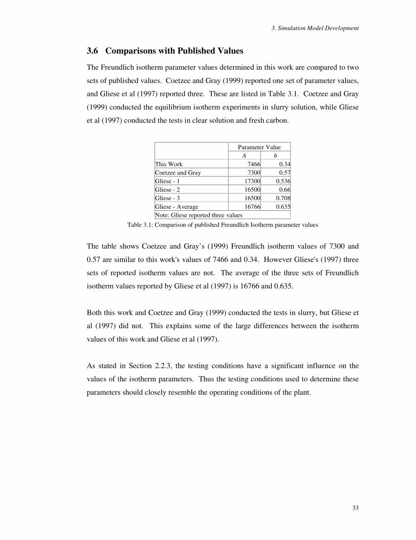
3. Simulation Model Development
33
3.6 Comparisons with Published Values
The Freundlich isotherm parameter values determined in this work are compared to two
sets of published values. Coetzee and Gray (1999) reported one set of parameter values,
and Gliese et al (1997) reported three. These are listed in Table 3.1. Coetzee and Gray
(1999) conducted the equilibrium isotherm experiments in slurry solution, while Gliese
et al (1997) conducted the tests in clear solution and fresh carbon.
Parameter Value A b This Work 7466 0.34Coetzee and Gray 7300 0.57Gliese - 1 17300 0.536Gliese - 2 16500 0.66Gliese - 3 16500 0.708Gliese - Average 16766 0.635Note: Gliese reported three values
Table 3.1: Comparison of published Freundlich Isotherm parameter values
The table shows Coetzee and Gray’ s (1999) Freundlich isotherm values of 7300 and
0.57 are similar to this work's values of 7466 and 0.34. However Gliese's (1997) three
sets of reported isotherm values are not. The average of the three sets of Freundlich
isotherm values reported by Gliese et al (1997) is 16766 and 0.635.
Both this work and Coetzee and Gray (1999) conducted the tests in slurry, but Gliese et
al (1997) did not. This explains some of the large differences between the isotherm
values of this work and Gliese et al (1997).
As stated in Section 2.2.3, the testing conditions have a significant influence on the
values of the isotherm parameters. Thus the testing conditions used to determine these
parameters should closely resemble the operating conditions of the plant.

34
4. Experimental Apparatus and Operation
The CIP plant experimental apparatus and its operations are described.
4.1 Introduction
This chapter will provide a detailed description of the experimental apparatus and its
operations. The specifications of all the equipment used are compiled in Appendix C.
4.2 Pilot Plant Apparatus
The CIP pilot plant consists of a feed agitator stand, six adsorption tanks, an adsorption
train support stand, agitators for the tanks and the feed drum, and three peristaltic
pumps. A photograph of the apparatus is shown in Figure 4.1 and a schematic is shown
in Figure 4.2.
The feed agitator stand provides support for the agitator of the feed drum. The stand is
approximately 3m high with a chain block at the top of the support stand used to hoist
the drum agitator in and out of the drum. Such an arrangement avoids the need to
unbolt the agitator from the stand every time the drum needs to be replaced and more
importantly, removes any heavy lifting from the operation.
The feed drum is a 200L plastic drum and sits on a pallet, allowing it to be moved
around the CIP pilot plant area with relative ease using a pallet truck. Another 200L
drum is used to collect the “ tailings” of the apparatus and it is located near Tank 6.
Three peristaltic pumps were used to pump solution through the apparatus. One pump
is used to pump the pulp from the feed drum into Tank 1. Another is used to pump the
“ tailings” from Tank 6 to a tailings drum. The third peristaltic pump is a multi-head
pump used as dosing pump to add gold and cyanide solutions to the apparatus.
The tanks are constructed of 304 stainless steel and are identical in size and
construction. The tanks have a nominal capacity of 50L and have a live working
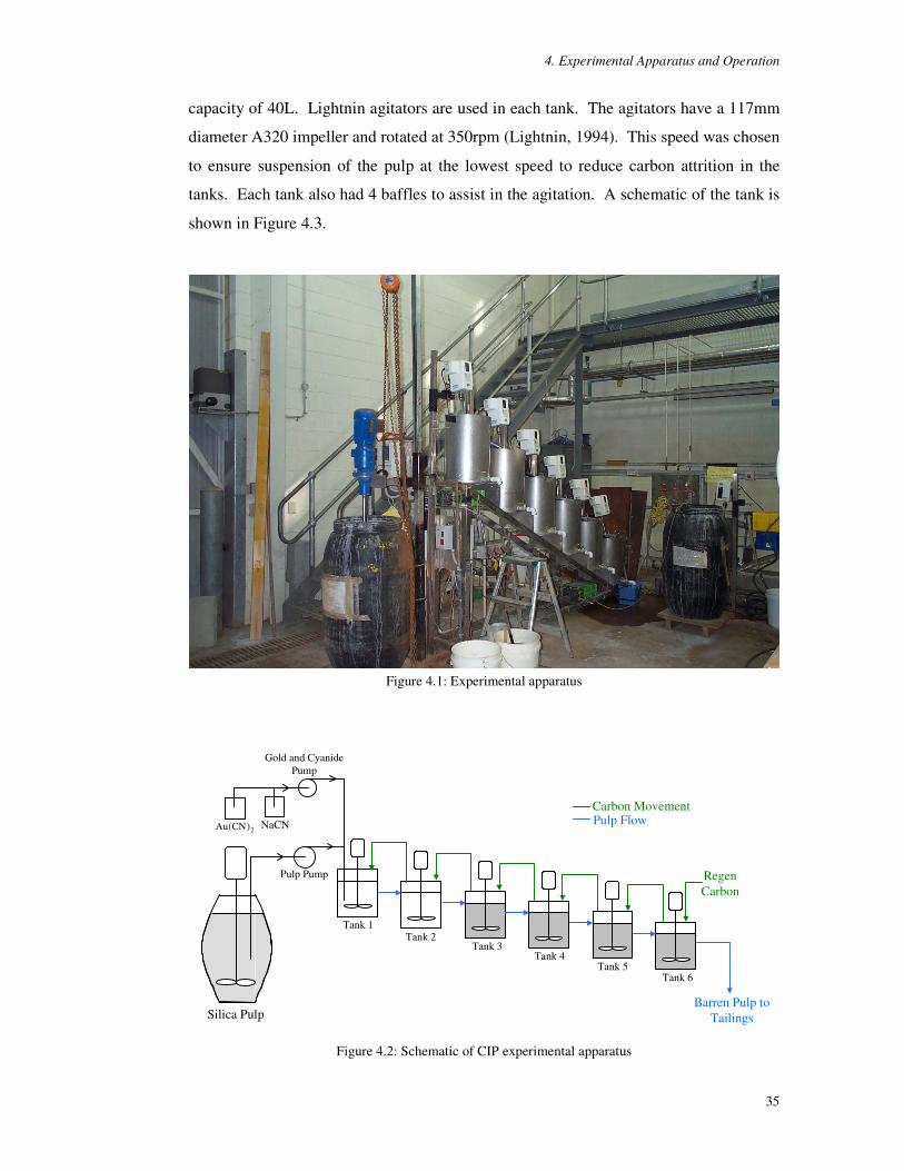
4. Experimental Apparatus and Operation
35
capacity of 40L. Lightnin agitators are used in each tank. The agitators have a 117mm
diameter A320 impeller and rotated at 350rpm (Lightnin, 1994). This speed was chosen
to ensure suspension of the pulp at the lowest speed to reduce carbon attrition in the
tanks. Each tank also had 4 baffles to assist in the agitation. A schematic of the tank is
shown in Figure 4.3.
Figure 4.1: Experimental apparatus
2)CN(Au NaCN
Silica PulpBarren Pulp to
Tailings
Pulp Pump
Gold and CyanidePump
RegenCarbon
Carbon MovementPulp Flow
Tank 1Tank 2
Tank 3Tank 4
Tank 6Tank 5
Figure 4.2: Schematic of CIP experimental apparatus
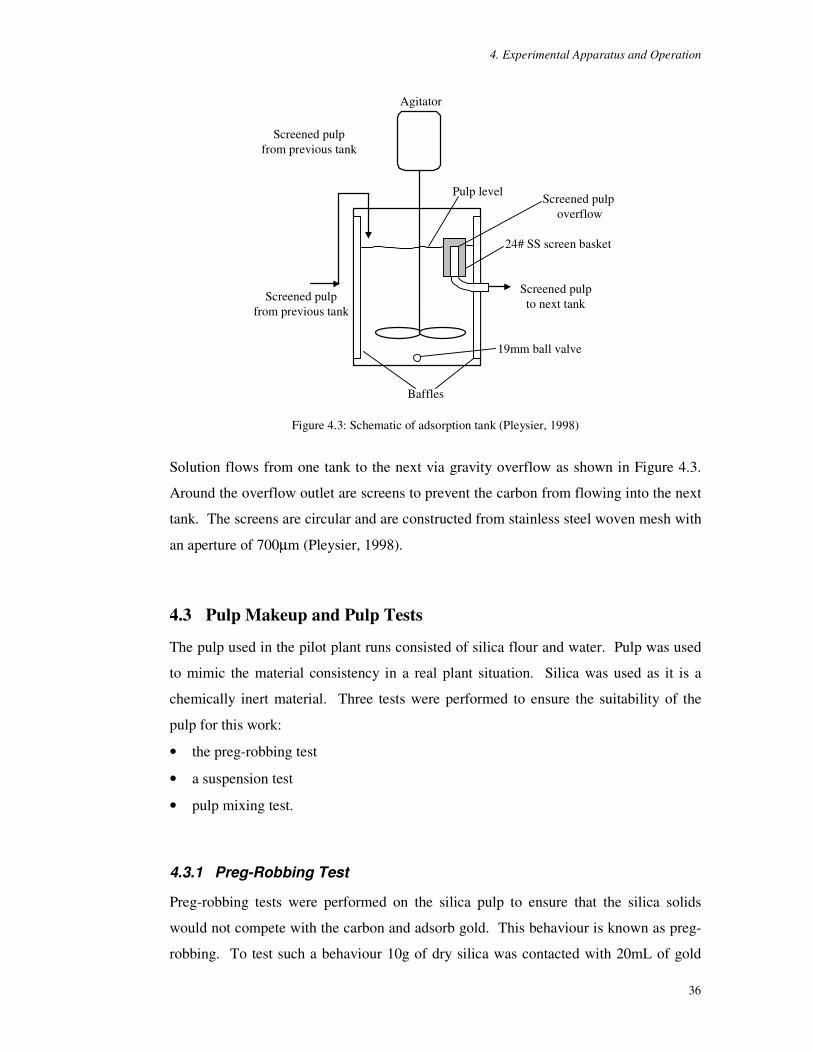
4. Experimental Apparatus and Operation
36
Agitator
Baffles
Screened pulpfrom previous tank
Screened pulpto next tankScreened pulp
from previous tank
24# SS screen basket
Pulp level Screened pulp overflow
19mm ball valve
Figure 4.3: Schematic of adsorption tank (Pleysier, 1998)
Solution flows from one tank to the next via gravity overflow as shown in Figure 4.3.
Around the overflow outlet are screens to prevent the carbon from flowing into the next
tank. The screens are circular and are constructed from stainless steel woven mesh with
an aperture of 700µm (Pleysier, 1998).
4.3 Pulp Makeup and Pulp Tests
The pulp used in the pilot plant runs consisted of silica flour and water. Pulp was used
to mimic the material consistency in a real plant situation. Silica was used as it is a
chemically inert material. Three tests were performed to ensure the suitability of the
pulp for this work:
• the preg-robbing test
• a suspension test
• pulp mixing test.
4.3.1 Preg-Robbing Test
Preg-robbing tests were performed on the silica pulp to ensure that the silica solids
would not compete with the carbon and adsorb gold. This behaviour is known as preg-
robbing. To test such a behaviour 10g of dry silica was contacted with 20mL of gold
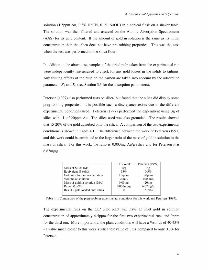
4. Experimental Apparatus and Operation
37
solution (1.5ppm Au, 0.3% NaCN, 0.1% NaOH) in a conical flask on a shaker table.
The solution was then filtered and assayed on the Atomic Absorption Spectrometer
(AAS) for its gold content. If the amount of gold in solution is the same as its initial
concentration then the silica does not have pre-robbing properties. This was the case
when the test was performed on the silica flour.
In addition to the above test, samples of the dried pulp taken from the experimental run
were independently fire assayed to check for any gold losses in the solids to tailings.
Any fouling effects of the pulp on the carbon are taken into account by the adsorption
parameters K2 and K3 (see Section 3.3 for the adsorption parameters).
Petersen (1997) also performed tests on silica, but found that the silica did display some
preg-robbing properties. It is possible such a discrepancy exists due to the different
experimental conditions used. Petersen (1997) performed the experiment using 3g of
silica with 1L of 20ppm Au. The silica used was also grounded. The results showed
that 15-20% of the gold adsorbed onto the silica. A comparison of the two experimental
conditions is shown in Table 4.1. The difference between the work of Petersen (1997)
and this work could be attributed to the larger ratio of the mass of gold in solution to the
mass of silica. For this work, the ratio is 0.003mg Au/g silica and for Petersen it is
6.67mg/g.
This Work Petersen (1997) Mass of Silica (Ms) Equivalent % solids Gold in solution concentration Volume of solution Mass of gold in solution (MAu) Ratio MAu/Ms Result - gold loaded onto silica
10g 33%
1.5ppm 20mL
0.03mg 0.003mg/g
0
3g 0.3%
20ppm 1000mL
20mg 6.67mg/g 15-20%
Table 4.1: Comparison of the preg-robbing experimental conditions for this work and Petersen (1997).
The experimental runs on the CIP pilot plant will have an inlet gold in solution
concentration of approximately 4-5ppm for the first two experimental runs and 9ppm
for the third run. More importantly, the plant conditions will have a %solids of 40-43%
- a value much closer to this work’ s silica test value of 33% compared to only 0.3% for
Petersen.

4. Experimental Apparatus and Operation
38
4.3.2 Pulp Suspension Tests
Pulp suspension tests were performed on the silica pulp to ensure that it remained in
suspension. The silica settled extremely quickly and had to be kept in suspension at all
times. This check was performed by probing around the edges of the tank, especially in
the baffles area, to ensure that there was no build up of solids at the bottom of the tank.
The pulp makeup in the test was the same as that used in the pilot plant run. This test
was performed to determine the optimal agitator speed and also performed periodically
during the experimental runs. The pulp suspension was also tested by checking the
% solids in the tank. This was performed when testing the pulp and carbon mixing
detailed in Section 4.3.3.
4.3.3 Pulp and Carbon Mixing Test
This test was performed to ensure the carbon and pulp were well mixed in the pilot plant
tanks. The pulp and carbon mixing test was performed in a single agitated tank. Again
the pulp makeup and the amount of carbon were the same as that for the pilot plant runs.
While the agitator remained on, the pulp was drained from the tank via the tap at the
bottom of the tank. It was observed that the amount of carbon removed from the first
20L of solution was the same as for the last 20L of solution. Hence, the carbon
distribution in the tank was homogeneous. The pulp % solids was also checked in this
experiment and it was found that the % solids for the first 20L was the same as that for
the last 20L.
4.4 Pilot Plant Operation
A typical pilot plant operation, runs for 24h/day. The feed solution, consisting of pulp,
gold cyanide and sodium cyanide solutions, were pumped into tank 1 via two peristaltic
pumps and traversed down the CIP pilot plant via gravity overflow. As the pulp flowed
out of Tank 6, the “ tailings” was collected in a small container and then pumped into an
empty drum.
The first peristaltic pump was used to pump the pulp into Tank 1. The pulp was stored
in a 200L drum and was continuously agitated. This pulp solution was pumped into
Tank 1 at a nominal rate of 8L/h. This flowrate was based on the capacity of the drum

4. Experimental Apparatus and Operation
39
for 24h. This flowrate was measured at the beginning and at the end of the CIP plant
runs to obtain a more accurate value to use in the simulation and calculations.
The pilot plant pulp feed composition of silica flour and water was maintained at 40-
43% solids. This pulp density was continually monitored throughout the run. It was
measured twice a day for every tank during carbon transfers using a Marcy scale. The
percentage solids value used in the simulations is the average value for all the
measurements taken. The pH of the drum and all the tanks were also measured twice a
day and maintained at 9.5 or higher. Caustic soda was used to maintain the pH in the
apparatus.
250ppm gold cyanide solution and 10000ppm sodium cyanide solution were pumped
into Tank 1 via a multi-head peristaltic pump at 2mL/min to yield a nominal feed gold
in solution concentration of 4.2ppm and to maintain a sodium cyanide concentration of
approximately 120-160ppm in each tank. This level of sodium cyanide concentration
closely mimics industrial practice. The sodium cyanide concentration was checked for
Tanks 1 and 6 twice a day.
At the start of an experimental run all the tanks were filled with barren pulp solution and
pre-loaded carbon was used for the first experimental run. This was initially put into
Tanks 1 to 5 and new carbon was put into Tank 6. This was done to reduce the amount
to time needed for the carbon loading to reach a steady state during the pilot plant
operation.
4.4.1 Carbon Transfer
In a real plant situation, carbon is normally transferred by pumping a certain amount of
pulp solution from tank to tank. As the pulp (and carbon) is pumped up the tank train,
the carbon is retained in the ‘higher’ tank while the solution flows back into the original
tank from which it was pumped. Hence there is mixing of pulp solution during carbon
transfer from two adjacent tanks. A detailed description of this carbon transfer method,
called the sequential-pull is described in Section 7.4.1.
For the first pilot plant run, the carbon was transferred using the carousel carbon
transfer method (which is described in more detail in Section 7.4.1). During carbon
4. Experimental Apparatus and Operation
40
transfer, the solution feed into the CIP pilot plant was firstly turned off. Carbon was
transferred from one tank to the next by draining the pulp solution from the tank via a
tap at the bottom of the tank and collecting the carbon in a sieve. The carbonless pulp
was then poured back into the tank and the carbon transferred up the tank train. This
carbon transfer procedure simulates the carousel carbon transfer method and does not
involve any mixing in the pulp solution for adjacent tanks during carbon transfers. The
loaded carbon was first removed from Tank 1, carbon was then transferred from Tank 2
to Tank 1 and so on down to Tank 6. New carbon was then added to the system in Tank
6. Once carbon transfer was completed, the solution feed to the CIP pilot plant was
turned back on.
This carbon transfer process took approximately 1.8h to complete. For the pilot plant
runs, carbon was transferred every 12h. This time period is referred to as the carbon
cycle time.
The amount of carbon transferred was measured by volume. The carbon was placed in
a 1L measuring cylinder and its volume was recorded. The mass of carbon transferred
was based on this volume measurement. The bulk density of carbon was determined in
a separate test where an amount of wet carbon was put into the measuring cylinder and
its volume recorded. It was then dried at 150°C and its dried mass recorded. The bulk
density of the carbon used in this work is 0.5517kg/L. This bulk density value was used
to determine the dry mass of the carbon transferred.
4.4.2 Carbon
The carbon used in the CIP pilot plant was regenerated carbon from Anglo Gold’ s
Sunrise Dam gold plant. It is Norit RO 3515 extruded carbon. By using regenerated
carbon, the effect of carbon fouling and the inherent inefficiencies of used carbon are
taken into account. In addition regenerated carbon is more representative of the type of
carbon used in a typical gold processing plant.

4. Experimental Apparatus and Operation
41
4.4.3 Sampling
Samples of both gold in solution and gold loading on carbon were taken at regular
intervals. As the behaviour of gold loading on carbon and the gold in solution
concentration were of most interest in the first three tanks, two samples were taken from
the first three tanks during every carbon cycle and one sample from the last three tanks.
Samples were taken on the fourth hour of the cycle for the first three tanks, and just
before carbon transfer for all tanks. The frequency of sampling was based on
Shannon’ s sampling theorem (Marlin, 1995). This calculation is shown in Appendix D.
Carbon samples of approximately 3g were taken. As a total of 9 samples were taken in
a single carbon cycle. An additional 30g was added to the amount of carbon added to
the system to compensate for the carbon removed during sampling. Hence the amount
of new carbon added to the system is 330g – 300g is the amount of carbon added to the
CIP system in Tank 6, and the 30g is the additional carbon added to compensate for
sampling. Carbon samples were dried, weighed, ashed, dissolved in aqua regia, diluted
and then analysed on a GBC 932 Atomic Adsorption Spectrometer (AAS).
Pulp samples size was approximately 80g. The samples were filtered, extracted into
DIBK and then analysed on the AAS.
The methods of analysis used are consistent with analytical techniques used in gold
plants.

42
5. Initial Pilot Plant Run
The initial pilot plant run was performed to obtain data to complete the
construction of the simulation model of the CIP process. The model was
then verified via an independent test.
5.1 Introduction
This chapter describes the final development of the simulation model using the results
of the first pilot plant run. Firstly the operating conditions of the pilot plant run are
detailed. Then the data collated from the experimental run is used to determine the
value of the adsorption rate parameters K2 and K3. This is detailed in Sections 5.3 to
5.5. The analysis of the simulated results of the pilot plant run is detailed in Section 5.6.
To independently verify this model, a batch test was performed and this is presented in
Section 5.7, and finally conclusions are presented in Section 5.8.
5.2 CIP Plant Operating Conditions
For the initial pilot plant run, the plant was operated for 5 days, running for 24
hours/day. A summary of the operational data of the CIP pilot plant is listed in Table
5.1.
The carbon was transferred every 12h. This time period is referred to as the carbon
cycle time. During this cycle time, the pilot plant operated for 10.2h and the inlet flow
was then turned off during the carbon transfer period of 1.8h. After this time the flow
was turned back on to start a new cycle.
The pulp flow rate entering the CIP pilot plant was 8.18L/h and its average percentage
solids during the experimental run was 40.3%. The gold in solution concentration was
4.2ppm. This was determined by the analysis of the feed solution.

5. Initial Pilot Plant Run
43
Pilot Plant Operating Data Total operation time Time period for each cycle Number of carbon transfers
5 days 12h, 10.2h operation and 1.8h carbon transfers (0.3h for each tank) 10
Feed Pulp Pulp makeup Pulp Flowrate % solids % solids in simulation pH Gold Solution Feed solution concentration and rate Actual gold feed concentration Cyanide Solution Sodium cyanide solution concentration Target NaCN concentration in tanks Flowrate
Silica flour and water 8.18L/h maintained at 40-43% 40.3% >9.5 in drum and all tanks 250ppm Au at 2mL/min 4.2ppm 10000ppm NaCN 120-160ppm 2mL/min
Residence Time Solution Carbon
5h in each tank, 30h in CIP apparatus 12h in each tank, 3 days in CIP apparatus
Carbon Data Concentration at the start of apparatus Mass of new carbon entering the apparatus Carbon Movement Amount of carbon transferred
nominal 10g/L (400g/tank) 300g + 30g to compensate for sampling Carousel carbon transfer ‘pull’ method, T1 out, T2 7�����7� 7���1Hw carbon in T6 100% carbon transfer
Sampling Tanks 1-3 Tanks 4-6
2 samples per cycle, 4th hour and before transfer 1 sample per cycle, taken before carbon transfer
Initial Conditions Gold Loading on Carbon (Used pre-loaded carbon) Gold in Solution Concentration
Tank 1 = 1043g/t Tank 2 = 890g/t Tank 3 = 680g/t Tank 4 = 547g/t Tank 5 = 429g/t Tank 6 = 133g/t 0ppm for all tanks
Table 5.1: Summary of CIP pilot plant operating data
All the tanks initially had nominally 400g of activated carbon. As the carbon was
transferred, only 330g of new carbon was put into Tank 6. This was done so that a
change could be observed in the system during the experiment. For this pilot plant run,
100% of the carbon in each tank was transferred.

5. Initial Pilot Plant Run
44
The initial gold in solution concentration for all the tanks was 0ppm. Preloaded carbon
was initially put into the Tanks 1 to 5 at the beginning of the run. The gold loading on
the preloaded carbon are listed in Table 5.1. The initial gold loading on carbon for Tank
6 is the loading of the new carbon put into the CIP pilot plant during operation.
5.3 Determining the Values of the Adsorption Rate Parameters
The final step in completing the simulation model was the determination of the
adsorption rate parameters K2 and K3 as described in Equations (3.3) and (3.4). The
parameters were determined using gPROMS gEST Parameter Estimation Tool (Process
Systems Enterprise, 1998). This involves the determination of the unknown value of
parameters in a mathematical model such that the probability that the mathematical
model will predict the values obtained from experiments is maximised (Process Systems
Enterprise, 2001). The objective function that is used to quantify this is given in
Equation (5.1). This is actually achieved by minimising the weighted difference
between the measured and predicted values across a number of experiments and is
expressed mathematically as:
( ) ( )
−++=Φ ∑∑ ∑
= = =
NE
i
NV
j
NM
k ijk
ijkijkijk
i ij zzN
1 1 12
22 )~(
lnmin21
2ln2
(5.1)
Where:
N Total number of measurements taken during all the experiments.
θ Set of model parameters to be estimated.
NE Number experiments performed.
NVi Number of variables measured in the ith experiment.
NMij Number of measurements of the jth variable in the ith experiment. 2ijk Variance of the kth measurement of variable j in experiment i.
ijkz~ kth measured value of variable j in experiment i.
ijkz kth (model-) predicted value of variable j in experiment i.
(Process Systems Enterprise, 2001)

5. Initial Pilot Plant Run
45
The first term of the objective function is a constant value for a given set of
measurements and does not change with different parameter estimation runs. The
second term, the sum of the variance terms ( 2ijk ), is dependent on the value of the
variance assigned for that particular variable for an estimation run. The final term, the
sum of the residuals, is the most influential term within the objective function. It is this
term that has the largest contribution to the value of the objective function.
The value N refers to the total number of measurements taken. These measurements
were the measured values of gold on carbon and gold in solution concentrations taken
from the pilot plant run and they are listed in Appendix E. NE is the number of
experiments performed and for this case it was one. NV is the number of variables
measured in the experiment. For this case it was 12 variables, gold loading on carbon
and gold in solution concentrations for 6 tanks. NM is the number of measurements for
each variable and they are listed in Appendix E. 2ijk is the variance of the variable. ijkz~
and ijkz are the measured and predicted values of the variables respectively.
Five parameter estimation runs were performed to determine the values of K2 and K3
and the results are listed in Table 5.2. The weightings given to the measured variables
were the difference between the runs. This weighting value, σijk, is the variance of the
measurement. Although the ‘weighting factor’ , σijk, is strictly the variance assigned in
each measured variable, in this work it is treated as an adjustable parameter. This
allowed various levels of importance to be assigned to different variables in the model
fitting. Values were chosen to reflect the desire to weight the gold on carbon and gold
in solution differently, as well as being cognisant of the errors (variance) in each
measurement. Estimates of the errors are described in Appendix E. Different
weightings were used to examine the sensitivity of the estimated parameter to changes
in the weighting values used. Hence multiple parameter estimation runs were
performed to determine the best combination of weightings assigned to the measured
variables, and as a consequence the best value of K2 and K3.
The value of the weightings assigned to the measured variables directly affects the
magnitude of the objective function and as such no comparison can be made between
the values of the objective function for each parameter estimation run.

5. Initial Pilot Plant Run
46
Tank 1 Tank 2 Tank 3 Tank 4 Tank 5 Tank 6 σijk Y 100 55 30 18 16 9 Xout 0.023 0.002 0.0065 0.0045 0.004 0.0045
gEST 1-1
Results: K2 = 341.99 K3 = -0.168
Objective Function = 14745
Tank 1 Tank 2 Tank 3 Tank 4 Tank 5 Tank 6
σijk Y 100 100 100 100 100 100 Xout 0.1 0.02 0.02 0.02 0.02 0.02
gEST 1-2
Results: K2=345.01 K3=-0.168
Objective Function = 542.53
Tank 1 Tank 2 Tank 3 Tank 4 Tank 5 Tank 6
σijk Y 100 100 100 100 100 100 Xout 0.08 0.02 0.008 0.008 0.008 0.008
gEST 1-3
Results: K2 = 343.54 K3 = -0.175
Objective Function = 715.29
Tank 1 Tank 2 Tank 3 Tank 4 Tank 5 Tank 6
σijk Y 100 100 100 100 100 100 Xout 0.008 0.02 0.008 0.008 0.008 0.008
gEST 1-4
Results: K2 = 349.91 K3 = -0.148
Objective Function = 1612.5
Tank 1 Tank 2 Tank 3 Tank 4 Tank 5 Tank 6
σijk Y 50 50 50 50 50 50 Xout 0.08 0.02 0.008 0.008 0.008 0.008
gEST 1-5
Results: K2 = 342.14 K3 = -0.168
Objective Function = 959.74
Note: Y: Gold on Carbon [mg/kg] Xout: Gold in Solution [ppm]
Table 5.2: Parameter Estimation Set 1 Results - Estimating K2 and K3
Once a parameter estimation has been performed, the gPROMS gEST tool will output
its optimal value for the parameter or parameters in question (in this case K2 and K3),
based on the weighting constraints assigned to the measured variables. gPROMS also
outputs a list of the predicted and actual values for the optimal values of the parameters
and other statistical information of the goodness of fit. The estimated parameter values
are then put into the pilot plant simulation model, modelled and the results are then
plotted and analysed. It is these results that are used to ascertain the effectiveness of the
weightings assigned and hence the most optimal K2 and K3 value.

5. Initial Pilot Plant Run
47
For the first parameter estimation run, gEST 1-1, weightings were chosen to ensure that
the residual errors of each of the variables were of a similar magnitude ranging from 5
to 6 (see Table 5.3). This residual error is given by Equation (5.2).
2
2
2
2 )~()(Error Residual
ijk
ijkijk zz
weightingsimulatedmeasured −
=−= (5.2)
The resultant K2 and K3 values for gEST 1-1 are 341.99 and -0.168 respectively. These
values of K2 and K3 were then used in the simulation model and the results of the
simulation are shown in Figure 5.1. The results consist of plots of the data collected
from the CIP pilot plant, and the simulated results for the gold loading on carbon (Y)
and the gold in solution concentration (Xout) for all tanks. The experimental data are
plotted with error bars. The errors were calculated based on the errors associated with
the analysis of gold in solution and gold loading on carbon. The errors are detailed in
Appendix E. For brevity, only the results from Tanks 1 and 2 are shown. The complete
set of results for every parameter run can be found in Appendix F.
The results show that the simulated data consistently under-predicts the gold on carbon
values for all tanks. This is also confirmed in Table 5.3. This table shows the measured
and simulated data, the residual errors (see Equation (5.2)) and the percentage errors
between the measured and simulated data. The measured data are the gold loading on
carbon (Y) and gold in solution concentration (Xout) at the period just before the carbon
is transferred. The table lists the average measured values for all the tanks when the
mass of carbon is at 0.3kg. (Note: The mass of carbon in the pilot plant was 0.4kg at the
start of the pilot plant run for Tanks 1 to 5, and 0.3kg was put into the system via Tank
6. As the experiment proceeded, 0.3kg of carbon was transferred, eventually leading to
0.3kg being present in each tank). The simulation values listed are the Y and Xout
values at the end of the simulation at 118.2h, the time before carbon transfer of the final
cycle.

5. Initial Pilot Plant Run
48
0
500
1000
1500
2000
0 20 40 60 80 100 120
Time [h]
Tank
1G
old
on C
arbo
n [m
g/kg
]
0
200
400
600
800
1000
1200
0 20 40 60 80 100 120
Time [h]
Tank
2G
old
on C
arbo
n [m
g/kg
]0.0
0.2
0.4
0.6
0.8
0 20 40 60 80 100 120
Time [h]
Tank
1G
old
in S
olut
ion
[pp
m]
0.0
0.1
0.2
0.3
0.4
0.5
0 20 40 60 80 100 120
Time [h]
Tank
2G
old
in S
olut
ion
[pp
m]
Figure 5.1: gEST 1-1 Results for Tanks 1 and 2. : Simulation, � Measured data.
Gold Loading on Carbon (Y) [mg/kg]
Tank 1 Tank 2 Tank 3 Tank 4 Tank 5 Tank 6 Measured Data1 1292 390 220 179 172 155 Simulated Data2 1054 267 149 135 133 133 Weighting 100 55 30 18 16 9 Residual Error 5.68 4.97 5.67 5.94 5.96 5.86 % difference 18.4% 31.5% 32.4% 24.5% 22.7% 14.1%
Gold in Solution Concentration (Xout) [ppm] Tank 1 Tank 2 Tank 3 Tank 4 Tank 5 Tank 6
Measured Data1 0.704 0.105 0.032 0.013 0.010 0.010 Simulated Data2 0.709 0.098 0.012 0.002 0.0002 0.0001 Weighting 0.023 0.002 0.0065 0.0045 0.004 0.0045 Residual Error 0.04 12.43 9.09 5.62 6.04 5.29 % difference -0.65% 6.71% 61.43% 84.22% 98.01% 99.04% Notes: 1. Average values of Y and Xout before carbon transfer for Mc = 0.3kg 2. Value at 118.2h of simulation
Table 5.3: gEST 1-1 Simulated Results - Estimating K2, K3 = 341.99, -0.168
Table 5.3 shows errors of 14% and more for gold loading on carbon values. The errors
for the gold in solution concentration values for the first two tanks are both under 7%,
but there are large percentage errors reported for the final four tanks. These high
percentage errors are not a true reflection of the actual error. Actual error values are
very low for Tanks 3-6 of 0.02ppm or less. In addition there are high errors associated
with the detection of low gold in solution values on the AAS.
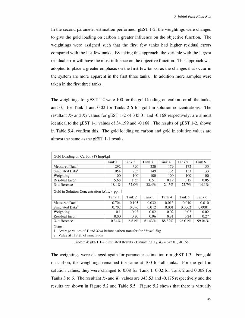
5. Initial Pilot Plant Run
49
In the second parameter estimation performed, gEST 1-2, the weightings were changed
to give the gold loading on carbon a greater influence on the objective function. The
weightings were assigned such that the first few tanks had higher residual errors
compared with the last few tanks. By taking this approach, the variable with the largest
residual error will have the most influence on the objective function. This approach was
adopted to place a greater emphasis on the first few tanks, as the changes that occur in
the system are more apparent in the first three tanks. In addition more samples were
taken in the first three tanks.
The weightings for gEST 1-2 were 100 for the gold loading on carbon for all the tanks,
and 0.1 for Tank 1 and 0.02 for Tanks 2-6 for gold in solution concentrations. The
resultant K2 and K3 values for gEST 1-2 of 345.01 and -0.168 respectively, are almost
identical to the gEST 1-1 values of 341.99 and -0.168. The results of gEST 1-2, shown
in Table 5.4, confirm this. The gold loading on carbon and gold in solution values are
almost the same as the gEST 1-1 results.
Gold Loading on Carbon (Y) [mg/kg] Tank 1 Tank 2 Tank 3 Tank 4 Tank 5 Tank 6 Measured Data1 1292 390 220 179 172 155 Simulated Data2 1054 265 149 135 133 133 Weighting 100 100 100 100 100 100 Residual Error 5.68 1.55 0.51 0.19 0.15 0.05 % difference 18.4% 32.0% 32.4% 24.5% 22.7% 14.1%
Gold in Solution Concentration (Xout) [ppm]
Tank 1 Tank 2 Tank 3 Tank 4 Tank 5 Tank 6 Measured Data1 0.704 0.105 0.032 0.013 0.010 0.010 Simulated Data2 0.702 0.096 0.012 0.001 0.0002 0.0001 Weighting 0.1 0.02 0.02 0.02 0.02 0.02 Residual Error 0.00 0.20 0.96 0.31 0.24 0.27 % difference 0.34% 8.61% 61.43% 88.32% 98.01% 99.04%
Notes: 1. Average values of Y and Xout before carbon transfer for Mc = 0.3kg 2. Value at 118.2h of simulation
Table 5.4: gEST 1-2 Simulated Results - Estimating K2, K3 = 345.01, -0.168
The weightings were changed again for parameter estimation run gEST 1-3. For gold
on carbon, the weightings remained the same at 100 for all tanks. For the gold in
solution values, they were changed to 0.08 for Tank 1, 0.02 for Tank 2 and 0.008 for
Tanks 3 to 6. The resultant K2 and K3 values are 343.53 and -0.175 respectively and the
results are shown in Figure 5.2 and Table 5.5. Figure 5.2 shows that there is virtually

5. Initial Pilot Plant Run
50
no change in the gold loading on carbon values but there is slightly better fit of the gold
in solution concentration across the tanks, particularly for Tank 2 where the errors
decreased from 7% for gEST 1-1 to 1% for gEST 1-3.
0
500
1000
1500
2000
0 20 40 60 80 100 120
Time [h]
Tank
1G
old
on
Car
bon
[mg/
kg]
0
200
400
600
800
1000
1200
0 20 40 60 80 100 120
Time [h]
Tan
k 2
Gol
d on
Car
bon
[mg/
kg]
0
0.2
0.4
0.6
0.8
0 20 40 60 80 100 120
Time [h]
Tank
1G
old
in S
olu
tion
[ppm
]0.00
0.10
0.20
0.30
0.40
0.50
0 20 40 60 80 100 120
Time [h]
Tank
2G
old
in S
olut
ion
[ppm
]
Figure 5.2: gEST 1-3 Results for Tanks 1 and 2. : Simulation, � Measured data
Gold Loading on Carbon (Y) [mg/kg] Tank 1 Tank 2 Tank 3 Tank 4 Tank 5 Tank 6 Measured Data1 1292 390 220 179 172 155 Simulated Data2 1054 270 150 135 133 133 Weighting 100 100 100 100 100 100 Residual Error 5.68 1.43 0.50 0.19 0.15 0.05 % difference 18.4% 30.7% 31.9% 24.5% 22.7% 14.1%
Gold in Solution Concentration (Xout) [ppm]
Tank 1 Tank 2 Tank 3 Tank 4 Tank 5 Tank 6 Measured Data1 0.704 0.105 0.032 0.013 0.010 0.010 Simulated Data2 0.731 0.104 0.013 0.002 0.0002 0.0001 Weighting 0.08 0.02 0.008 0.008 0.008 0.008 Residual Error 0.11 0.00 5.34 1.88 1.50 1.67 % difference -3.78% 1.00% 57.98% 86.58% 97.81% 99.04%
Notes: 1. Average values of Y and Xout before carbon transfer for Mc = 0.3kg 2. Value at 118.2h of simulation
Table 5.5: gEST 1-3 Simulated Results - Estimating K2, K3 = 343.54 and -0.175
Table 5.5 also shows that the contribution to the objective function of the gold in
solution values is larger for Tanks 3 to 6, compared with Tanks 1 and 2. This is due to
the larger relative errors in the gold in solution values. The contribution to the objective

5. Initial Pilot Plant Run
51
function for the gold on carbon is greater than that for the gold in solution, for all three
parameter estimations performed.
Two additional parameter estimations (gEST 1-4 and gEST 1-5) were performed to
increase the contribution to the objective function of some variables. For gEST 1-4 the
weighting for the gold in solution concentration for Tank 1 (T1.Xout) was reduced from
0.08 to 0.008. This resulted in an increased contribution of T1.Xout’ s residual error to
the objective function. The resultant K2 and K3 was 349.91 and -0.148 and the results
are shown in Table 5.6. These K2 and K3 values result in very low simulated gold in
solution values with errors for Tanks 1 and 2 of 12% and 28% respectively. These errors
are a significant increase over gEST 1-3 errors of less than 4% for both tanks. The
reason for this is due to the lower measured gold in solution values for Tank 1 for the
first three carbon cycles.
Gold Loading on Carbon (Y) [mg/kg]
Tank 1 Tank 2 Tank 3 Tank 4 Tank 5 Tank 6 Measured Data1 1292 390 220 179 172 155 Simulated Data2 1054 250 146 134 133 133 Weighting 100 100 100 100 100 100 Residual Error 5.68 1.95 0.55 0.20 0.15 0.05 % difference 18.4% 35.8% 33.8% 25.1% 22.7% 14.1%
Gold in Solution Concentration (Xout) [ppm] Tank 1 Tank 2 Tank 3 Tank 4 Tank 5 Tank 6
Measured Data1 0.704 0.105 0.032 0.013 0.010 0.010 Simulated Data2 0.618 0.075 0.009 0.001 0.0001 0.0001 Weighting 0.008 0.02 0.008 0.008 0.008 0.008 Residual Error 116.64 2.21 8.52 2.14 1.54 1.67 % difference 12.27% 28.32% 73.22% 92.42% 99.00% 99.04% Notes: 1. Average values of Y and Xout before carbon transfer for Mc = 0.3kg 2. Value at 118.2h of simulation
Table 5.6: gEST 1-4 Simulated Results - Estimating K2, K3 = 349.91, -0.148
The measured data indicates that the CIP pilot plant was slowly reaching the maximum
T1.Xout value of approximately 0.55ppm (for Mc = 0.4kg) over a number of cycles.
However in the simulated results this value is reached within the first cycle. This is
apparent in Figure 5.3. It is this ‘slow’ plant behaviour that results in the large T1.Xout
errors for the first three carbon cycles, which has a direct affect on the parameter
estimation values of K2 and K3 when a high contribution is placed on the measurement
of T1.Xout. Hence care must be taken not to place too high a contribution of T1.Xout.

5. Initial Pilot Plant Run
52
0
0.2
0.4
0.6
0.8
0 20 40 60 80 100 120
Time [h]
Tank
1G
old
in S
olut
ion
[ppm
]
Figure 5.3: gEST 1-4 Gold in solution concentration for Tank 1
: Simulation, � Measured data
The final parameter estimation run, gEST 1-5, was performed to attempt to obtain a
better fit for gold loading on carbon (Y) by reducing the weighting of the Y values to 50.
By reducing the weighting to 50, the residual error for the Y values increases and hence
has a larger impact on the objective function. The resultant K2 and K3 values for this
parameter estimation run are 342.14 and -0.182 respectively. Table 5.7 summaries the
results of this parameter estimation run.
Gold Loading on Carbon (Y) [mg/kg] Tank 1 Tank 2 Tank 3 Tank 4 Tank 5 Tank 6 Measured Data1 1292 390 220 179 172 155 Simulated Data2 1054 276 152 135 133 133 Weighting 50 50 50 50 50 50 Residual Error 22.73 5.16 1.87 0.77 0.61 0.19 % difference 18.4% 29.2% 31.0% 24.5% 22.7% 14.1%
Gold in Solution Concentration (Xout) [ppm]
Tank 1 Tank 2 Tank 3 Tank 4 Tank 5 Tank 6 Measured Data1 0.704 0.105 0.032 0.013 0.010 0.010 Simulated Data2 0.764 0.113 0.015 0.002 0.0003 0.0001 Weighting 0.08 0.02 0.008 0.008 0.008 0.008 Residual Error 0.56 0.16 4.46 1.78 1.49 1.67 % difference -8.46% -7.57% 52.97% 84.30% 97.31% 99.04% Notes: 1. Average values of Y and Xout before carbon transfer for Mc = 0.3kg 2. Value at 118.2h of simulation
Table 5.7: gEST 1-5 Simulated Results - Estimating K2, K3 = 342.14, -0.182
Reducing the weighting of the carbon to 50 has a small effect on the gold loading on
carbon for Tanks 2 and 3, where the gold on carbon values increased and its errors
decreased. It also increased the gold in solution values, particularly for the first two
tanks where its error increased from 4% in gEST 1-3 to 8%. It appears that changes in
5. Initial Pilot Plant Run
53
K2 and K3 have very little influence on the simulated values of Y, but do have a small
effect on Xout. Subsequent sensitivity analyses in Chapter 6 confirms this.
Results for Tanks 3-6 for all the parameter estimation runs for K2 and K3 are almost the
same. An examination of the plots in Appendix E confirms this.
In conclusion, the overall best fit of experimental data to predicted data was gEST 1-3
with K2 and K3 values of 343.54 and -0.175 respectively, using weightings of 100 for
gold on carbon for all tanks and 0.08 for Tank 1, 0.02 for Tank 2, and 0.008 for Tanks
3-6 for the gold in solution concentrations. The multiple parameter estimations
performed show that care must be taken in the choice of weightings used as it has a
direct impact on the value of the parameter being estimated. It appears that changes in
the values of K2 and K3 have little influence on the gold on carbon values, but does have
a small effect on the gold in solution values.
The fit of the model to plant data, although satisfactory for gold in solution, is
consistently under-predicting for gold on carbon. The next section describes the
additional parameter estimation analyses performed in order to overcome this under-
prediction of gold on carbon and to obtain a better fit of the mathematical model to the
experimental data.

5. Initial Pilot Plant Run
54
5.4 Further Parameter Estimations
This section details the work performed to find a better fit of the model to the CIP pilot
plant data, in particular the fit of simulated gold on carbon to the measured values. Four
sets of parameter estimation runs were performed. The first set involved estimating the
four parameter values of the model, K2 and K3, and the two Freundlich isotherm
parameters of A and b. The second involved the estimation of the gold in solution
concentration entering the adsorption process at Tank 1 (T1.Xin), the adsorption
parameters K2 and K3 and the percentage of solids material in the pulp (%solids). The
third set involved the estimation of the initial gold loading on the carbon entering the
system via Tank 6 (T6.Yin). The final set involved the estimation of K2 and K3 using
lower masses of carbon. All the parameter estimations performed used the same
weightings as gEST 1-3. Hence the weightings used were 100 for all the gold loading
on carbon variables, 0.08 for Tank 1, 0.02 for Tank 2 and 0.008 for Tanks 3 to 6 for the
gold in solution concentration variables.
5.4.1 Parameter Estimation of Adsorption Rate Parameters and
Freundlich Isotherm Parameters
Parameter estimation gEST 2-1 was the simultaneous estimation of adsorption rate
parameters K2 and K3, and the Freundlich isotherm parameters A, and b. The results are
shown in Table 5.8 and Table 5.9. The graphs of the simulated data using gEST 2-1
results have not been shown here but can be found in Appendix E. Although the values
of A and b have already been determined via independent equilibrium isotherm tests
(see Section 3.5 for details), it was decided to combine them into this parameter
estimation run to determine whether an optimal combination for K2 and K3, A, and b
could be achieved.
The estimated K2 and K3 values for gEST 2-1 are 343.36 and –0.175 respectively. The
A and b values are 14934 and 1.83×10⁻⁷ respectively, compared with 7466 and 1.34
from the independent equilibrium isotherm tests. The K2 and K3 values for gEST 2-1
are almost identical to gEST 1-3 results of 343.54 and –0.175 respectively. This is
confirmed in Table 5.9, which shows the comparison between measured and simulated
values for gEST 2-1. The gEST 1-3 results are also included for comparison. Table 5.9

5. Initial Pilot Plant Run
55
shows that the simulated gold loading on carbon and gold in solution concentration
values for gEST 1-3 and 2-1 are almost identical. This is also confirmed by the values
of their objection functions of 715 for gEST 1-3 and 718 for gEST 2-1.
gEST 2-1 Parameters Estimated: K2, K3, A, b Results: K2 = 343.36 Objective Function = 718.30 K3 = -0.175 A = 14934 b = 1.83×10⁻⁷
gEST 2-2 Parameters Estimated: K1, A, b Results: K1 = 144.56 Objective Function = 559.49 A = 24914 b = 1.172 Correlation between estimated parameters: K1 and A = -0.123 K1 and b = -0.039 A and b = 0.984
Table 5.8: Parameter Estimation Set 2 Results - Estimating K1, K2, K3, A, b
Gold Loading on Carbon (Y) [mg/kg] Tank 1 Tank 2 Tank 3 Tank 4 Tank 5 Tank 6 Measured Data1 1292 390 220 179 172 155 gEST 1-32 1054 270 150 135 133 133 gEST 2-12 (using K2 and K3) 1054 271 151 135 133 133 gEST 2-22 (using K1) 1051 249 148 135 133 133 % difference 1-4 & measured 18.4% 30.8% 31.8% 24.6% 22.7% 14.2% % difference 2-1 & measured 18.4% 30.5% 31.4% 24.6% 22.7% 14.2% % difference 2-2 & measured 18.7% 36.2% 32.7% 24.6% 22.7% 14.2%
Gold in Solution Concentration (Xout) [ppm]
Tank 1 Tank 2 Tank 3 Tank 4 Tank 5 Tank 6 Measured Data1 0.704 0.105 0.032 0.013 0.0100 0.0100 gEST 1-32 0.731 0.104 0.013 0.002 0.0002 0.0001 gEST 2-12 (using K2 and K3) 0.733 0.104 0.013 0.002 0.0002 0.0001 gEST 2-22 (using K1) 0.603 0.095 0.023 0.013 0.0117 0.0116 % difference 1-4 & measured -3.8% 1.0% 58.1% 86.9% 97.8% 99.0% % difference 2-1 & measured -4.1% 1.0% 58.1% 86.9% 97.8% 99.0% % difference 2-2 & measured 14.3% 9.5% 27.5% -0.8% -17.0% -15.5% Notes: 1. Average values of Y and Xout before carbon transfer for Mc = 0.3kg 2. Value at 118.2h of simulation
Table 5.9: Parameter Estimation Set 2 Simulated Results - Estimating K1, K2, K3, A, b
Although an optimal solution was found for gEST 2-1, gPROMS was unable to provide
the statistical information as for previous parameter estimations, stating that this was

5. Initial Pilot Plant Run
56
possibly due to some of the parameters being highly correlated. Further investigation
revealed this to be true. In the previous set of parameter estimation in Section 5.3, the
parameter values of K2 and K3 were highly correlated with correlation coefficients of
–0.997 for all five parameter estimations performed.
Another parameter estimation (gEST 2-2) was performed whereby K1 was estimated
instead of K2 and K3. The relationship between these three parameters is governed by
Equations (3.3) and (3.4) which are reproduced below.
)X(XKR eout −= 1 (3.3)
321
KYKK = (3.4)
If K1 is used in the model, then the K2 and K3 are not used. Hence for gEST 2-2, K1 was
estimated with A and b and the resultant parameter values are 144.56, 24914 and 1.172
respectively. The results are shown in Table 5.8 and Table 5.9. Again the A and b
values are very different from the values obtained from the equilibrium isotherm tests.
The results also show a very high correlation between the two isotherm parameters with
correlation coefficient values of 0.98 (see Table 5.8 for correlation between the
estimated parameters).
The simulated results of gEST 2-2 show the gold loading on carbon is still being under-
predicted and are similar to those reported for gEST 1-3, with Tank 2 errors 6% higher
for gEST 2-2. Gold in solution simulation values are lower than the actual values for
Tanks 1-3, particularly for Tank 1 where the simulated value is 0.6ppm compared with
0.7ppm for the experimental data. For Tanks 4-6, the gold in solution values seem to
level off to a value of approximately 0.01ppm (see Figure 5.4). These simulated values
are consistently higher than the actual values even though they lie within the error bars
of the actual data. This behaviour is very different from gEST 1-3 where the gold in
solution results were very low with values between 0.0001ppm and 0.002ppm.
This behaviour also results in a reduction of the objective function for gEST 2-2 of 559,
compared with 715 for gEST 1-3. A smaller objective function usually indicates an
improvement of the fit of simulated data to the measured data. However this is not the

5. Initial Pilot Plant Run
57
case for gEST 2-2. This lower objective function for gEST 2-2 is due to the lower
errors of the gold in solution concentrations for Tanks 3 to 6.
In a simulated environment one would expect all of the gold to be adsorbed onto the
carbon leaving very little going out to tailings. This is the case for gEST 1-3. However
in reality, due to physical limitations of analytical techniques used to measure the gold
in solution concentrations, readings of less than 0.01ppm are difficult to detect and the
measured value of gold in solution concentrations for Tanks 5 and 6 are in this vicinity.
Such a value would not be expected for a simulation where such constraints are not
present. Hence, while the objective function has been reduced because of the improved
fit of the simulated gold in solution values for Tanks 3 to 6 to its measured values, this
improvement is more apparent than real. No significant improvement has been gained
in Tanks 1 and 2. Overall, the fit of simulated data to the measured data for gEST 2-1
and 2-2 is not a significant improvement over gEST 1-3.
0
0.01
0.02
0.03
0.04
0.05
0 20 40 60 80 100 120
Time [h]
Gol
d in
Sol
utio
n [p
pm]
Tank 4 Tank 5 Tank 6
T4-measured T5-measured T6-measured
Note: Error bars shown on Tank 5 measured values only
Figure 5.4: gEST 2-1 - Gold in solution concentrations for Tanks 4 to 6
5.4.2 Parameter Estimation of Gold in Solution Entering Tank 1,
Adsorption Rate Parameters and Percentage Solids
The second set of additional parameter estimations performed was to estimate
combinations of gold in solution concentration entering the CIP pilot plant in the first
tank (T1.Xin), the rate of adsorption parameters (K2 and K3) and the percentage of solids
(by weight) in the pulp (%solids). Two parameter estimations were performed. gEST
3-1 involved the parameter estimations of K2 and K3 and T1.Xin, and gEST 3-2 involved
the parameter estimations of K2 and K3, T1.Xin and % solids. The results of both

5. Initial Pilot Plant Run
58
parameter estimations performed are summarised in Table 5.10. The simulated results
are tabulated in Table 5.11. The results of gEST 1-3 are also included for comparison.
gEST 3-1 estimated the values of K2, K3, and T1.Xin and the results are 353.57, -0.148
and 5.11ppm respectively. The estimated value of T1.Xin of 5.11ppm is higher than that
used in gEST 1-3 of 4.2ppm. The objective function for gEST 3-1 of 698 is lower than
gEST 1-3 (715), suggesting a better fit of the simulated results to the measured data and
the results in Table 5.11 confirms this. There is a better fit of simulated gold loading on
carbon for Tank 1 for gEST 3-1 compared with gEST 1-3 with the errors between the
measured and simulated data decreasing from 18.4% to 3%. The errors of the gold in
solution concentration values for Tanks 1 and 2 increased for gEST 3-1 compared to
gEST 1-3. The higher T1.Xin estimation result indicate that it is possible that there may
be a higher degree of error than initially expected for the measured T1.Xin value of
4.2ppm used in the CIP pilot plant model.
gEST 3-1 Parameters Estimated: K2, K3, T1.Xin Results: K2 = 353.56 Objective Function = 698.29 K3 = -0.148 T1.Xin = 5.109ppm
Correlation between estimated parameters: K2 and K3 = -0.993 K2 and T1.Xin = -0.206 K3 and T1.Xin = 0.292
gEST 3-2 Parameters Estimated: K2, K3, T1.Xin, %solids Results: K2 = 339.82 Objective Function = 659.96 K3 = -0.137 T1.Xin = 4.143ppm %solids = 0
Correlation between estimated parameters: K2 and K3 = -0.994 K2 and T1.Xin = -0.226 K3 and T1.Xin = 0.308
Table 5.10: Parameter Estimation Set 3 Results - Estimating K2, K3, T1.Xin, %solids

5. Initial Pilot Plant Run
59
Gold Loading on Carbon (Y) [mg/kg]
Tank 1 Tank 2 Tank 3 Tank 4 Tank 5 Tank 6 Measured Data1 1292 390 220 179 172 155 gEST 1-3 1054 270 150 135 133 133 gEST 3-1 1253 277 149 135 133 133 gEST 3-2 1277 307 156 136 133 133 % difference 1-3 & measured 18.4% 30.8% 31.8% 24.6% 22.7% 14.2% % difference 3-1 & measured 3.0% 29.0% 32.3% 24.6% 22.7% 14.2% % difference 3-2 & measured 1.2% 21.3% 29.1% 24.0% 22.7% 14.2%
Gold in Solution Concentration (Xout) [ppm] Tank 1 Tank 2 Tank 3 Tank 4 Tank 5 Tank 6 Measured Data1 0.704 0.105 0.032 0.013 0.0100 0.0100 gEST 1-3 0.731 0.104 0.013 0.002 0.0002 0.0001 gEST 3-1 0.762 0.093 0.010 0.001 0.0001 0.0001 gEST 3-2 0.727 0.107 0.015 0.002 0.0003 0.0001 % difference 1-3 & measured -3.8% 1.0% 58.1% 86.9% 97.8% 99.0% % difference 3-1 & measured -8.2% 11.4% 67.5% 91.0% 98.6% 99.0% % difference 3-2 & measured -3.3% -1.9% 54.4% 84.9% 97.4% 99.0% Notes: 1. Average values of Y and Xout before carbon transfer for Mc = 0.3kg 2. gEST values are at 118.2h of simulation
Table 5.11: Parameter Estimation Set 3 Simulated Results - Estimating K, T1.Xin, %solids
The other parameter estimation run in this set, gEST 3-2, was performed on the gold in
solution concentration entering the pilot plant in first tank (T1.Xin), the rate of
adsorption parameters (K2 and K3) and the percentage of solids (by weight) in the pulp
(%solids). The results for K2, K3, T1.Xin, and %solids are 339.82, -0.137, 4.143ppm,
0% respectively.
The %solids value of 0 is not correct, as there were solids in the CIP pilot plant during
operation. In addition this was checked and maintained for the duration of the pilot
plant run.
An analysis of the amount of gold entering the system for gEST 3-1 (T1.Xin=5.109ppm)
and 3-2 (T1.Xin=4.143ppm) shows that this value for the two simulations are very
similar. The amount of gold entering the system per hour for gEST 3-1 and 3-2 are
33.21mg/h and 33.89mg/h respectively. Even though the T1.Xin values of gEST 3-1
and 3-2 are not the same, they both deliver a similar amount of gold into the system per
hour. This is because of the zero %solids in the pulp for gEST 3-2. Overall gEST 3-2
has the best fit of the simulated data to the measured values. Its lower objective
function value of 660 confirms this.

5. Initial Pilot Plant Run
60
In conclusion, the results of these two parameter estimations show that if the gold in
solution entering the system (T1.Xin) is increased, there is a better fit of gold loading on
carbon for Tank 1 and to a lesser extent Tank 2. Thus the under-prediction of gold on
carbon displayed in Section 5.3 could be due to the T1.Xin value used, suggesting that
there may be some error in the measured value of T1.Xin of 4.2ppm. An investigation
of this is detailed in Section 5.4.4.1. In addition, if the measured value of T1.Xin is
higher than the reported value of 4.2ppm, this will have an impact on the initial
parameter estimations of K2 and K3 detailed in Section 5.3.
5.4.3 Parameter Estimation of Gold Loading on Carbon Entering the CIP
System
Three parameter estimation runs were performed to investigate the amount of gold
loaded onto the carbon entering the system in Tank 6 (T6.Yin). This investigation was
undertaken to determine whether a change in the value of T6.Yin would improve the
simulated gold loading on carbon results when compared to the measured data. The
parameter estimations performed are labelled gEST 4-1 to gEST 4-3 and the results are
shown in Table 5.12. The simulated results are shown in Table 5.13.
gEST 4-1 Parameters Estimated: T6.Yin Results: T6.Yin = 237mg/kg Objective Function = 686.61
gEST 4-2 Parameters Estimated: K2, K3, T6.Yin Results: K2 = 342.19 Objective Function = 686.44 K3 = -0.171 T6.Yin = 235mg/kg
Correlation between estimated parameters: K2 and K3 = -0.998 K2 and T6.Yin = 0.092 K3 and T6.Yin = -0.082
gEST 4-3 Parameters Estimated: K2, K3, T6.Yin, T1.Xin Results: K2 = 348.02 Objective Function = 678.10 K3 = -0.152 T6.Yin = 221mg/kg T1.Xin = 4.83ppm
Correlation between estimated parameters: K2 and K3 = -0.995 K3 and T6.Yin = -0.148 K2 and T6.Yin = 0.140 K3 and T1.Xin = 0.334 K2 and T1.Xin = -0.261 T6.Yin and T1.Xin = -0.247
Table 5.12: Parameter Estimation Set 4 Results - Estimating T6.Yin

5. Initial Pilot Plant Run
61
Gold Loading on Carbon (Y) [mg/kg]
Tank 1 Tank 2 Tank 3 Tank 4 Tank 5 Tank 6 Measured Data1 1292 390 220 179 172 155 gEST 1-3 1054 270 150 135 133 133 gEST 4-1 1158 373 255 239 237 237 gEST 4-3 1280 364 238 223 222 221 % difference 1-3 & measured 18.4% 30.8% 31.8% 24.6% 22.7% 14.2% % difference 4-1 & measured 10.4% 4.4% -15.9% -33.5% -37.8% -52.9% % difference 4-2 & measured 0.9% 6.7% -8.2% -24.6% -29.1% -42.6%
Gold in Solution Concentration (Xout) [ppm] Tank 1 Tank 2 Tank 3 Tank 4 Tank 5 Tank 6 Measured Data1 0.704 0.105 0.032 0.013 0.0100 0.0100 gEST 1-3 0.731 0.104 0.013 0.002 0.0002 0.0001 gEST 4-1 0.718 0.104 0.014 0.002 0.0003 0.0001 gEST 4-3 0.751 0.099 0.012 0.002 0.0002 0.0001 % difference 1-3 & measured -3.8% 1.0% 58.1% 86.9% 97.8% 99.0% % difference 4-1 & measured -2.0% 1.0% 56.3% 84.9% 97.0% 99.0% % difference 4-3 & measured -6.7% 6.2% 61.9% 88.2% 97.8% 99.0% Notes: 1. Average values of Y and Xout before carbon transfer for Mc = 0.3kg 2. gEST values are at 118.2h of simulation
Table 5.13: Parameter Estimation Set 4 Simulated Results - Estimating T6.Yin
The first parameter estimation performed, gEST 4-1, was to estimate the most optimal
value of T6.Yin under the same simulating conditions as gEST 1-3. Thus the adsorption
rate parameters K2 and K3 were set to 343.54 and -0.175 respectively, and the gold in
solution entering the system was set at 4.2ppm. The resulting T6.Yin value was
237mg/kg, compared to 133mg/kg previously used.
The second parameter estimation run, gEST 4-2, was the simultaneous estimation of the
adsorption parameters, K2 and K3, and T6.Yin. The estimation results are 342.19, -0.171
and 235mg/kg for K2, K3, and T6.Yin respectively. These results are almost identical to
those of gEST 4-1 where the K2, K3, and T6.Yin used are 343.54 -0.175, 237mg/kg.
This is confirmed by the identical objective function for gEST 4-1 and 4-2 of 686.5.
The low correlation between T6.Yin and K2, and T6.Yin and K3, of less than 0.1, indicate
that T6.Yin is independent of both K2 and K3. This behaviour is also similar for T1.Xin
and K2 and K3. As the parameter estimation results for gEST 4-1 and 4-2 are the same,
only gEST 4-1 will be simulated and discussed.
The simulated results of gEST 4-1 (see Table 5.13) show that the gold in solution values
of gEST 4-1 are almost identical to gEST 1-3. The gold loadings on carbon values have
all increased by approximately 104mg/kg - the difference between T6.Yin for gEST 1-3
5. Initial Pilot Plant Run
62
of 133mg/kg and T6.Yin for gEST 4-1 of 237mg/kg. Hence increasing T6.Yin has little
effect on the gold in solution results.
The simulated results for gEST 4-1 for the gold loading on carbon show an
improvement in the fit of the simulated data to the measured data for the first three
tanks. For the first tank, the percentage error between the measured and simulated data
decreases from 18% for gEST 1-3, to 10% for gEST 4-1. For the second tank the
percentage error decreases from 31% to 4% and for Tank 3, it decreases from 32% to
16%. The percentage error, however, increases for the final three tanks, but for the first
time the simulated data for gold loading on carbon is higher than the measured value.
Using T6.Yin of 237mg/kg instead of 133mg/kg does provide an overall better fit of the
simulated data to the measured values based on the objective function. The objective
function using T6.Yin of 237mg/kg is 687 and for 133mg/kg it is 715.
The final parameter estimation performed in this set, gEST 4-3, was to estimate the best
combination of the gold loading on carbon entering the system (T6.Yin), the gold in
solution concentration entering the system (T1.Xin) and the two adsorption parameters.
The results for gEST 4-3 for K2, K3, T6.Yin, and T1.Xin are 348.02, -0.152, 221mg/kg
and 4.83ppm respectively. The simulated results for gEST 4-3 for the gold in solution
concentrations are within 0.02ppm of gEST 1-3, but the overall fit of gold loading on
carbon values is better. An analysis of the percentage errors and the value of the
objective function supports this. The percentage errors of gold loading on carbon for
the first three tanks are 8% or below, compared with 16% for gEST 4-1 and 32% for
gEST 1-3. The errors for Tanks 4 and 5 are similar to gEST 1-3 but the error for Tank 6
is higher at 43% compared with 14%.
The increase in T6.Yin from the original value of 133mg/kg (gEST 1-3) to the gEST 4-3
value of 221 mg/kg is 88mg/kg. From the simulated results it can be seen that the
increase in the gold loading on carbon values from gEST 1-3 values to gEST 4-3 values
is at minimum 88mg/kg. The increase in gold loading on the carbon from gEST 1-3 to
gEST 4-3 for Tank 1 is 226mg/kg, Tank 2 is 94mg/kg and Tanks 3 to 6 is about
88mg/kg. The larger increases for Tanks 1 and 2 can be attributed to the higher T1.Xin
used in gEST 4-3.

5. Initial Pilot Plant Run
63
In conclusion, these results show that it is possible that the initial gold loading on the
carbon entering the system may be higher than 133mg/kg. Increasing T6.Yin only will
increase the simulated gold loadings on the carbon values by the same corresponding
amount. The improved fit of gEST 4-3 results to the measured data again confirms that
the value of T1.Xin may be higher than its reported value and needs to be investigated.
5.4.4 Investigation of Errors in Simulated Results
Analysis of the results of the parameter estimations performed in previous sections
show that the simulated gold loading on carbon data consistently under-predicts the
measured data. Three items have been identified as being contributing factors to this
under-prediction and thus requiring further investigation. They are the concentration of
gold in solution entering Tank 1 (T1.Xin), the value of the initial gold loading on the
carbon entering the system in Tank 6 (T6.Yin) and the value of the mass of carbon used
in the simulation model.
5.4.4.1 Investigation of the Gold in Solution Concentration Entering Tank 1
The results presented in the parameter estimations in previous sections suggest that
there does not seem to be enough gold in the system. This is more apparent in the plots
of the gold on carbon values where the simulated values continually under-predict the
measured values.
This section will firstly investigate the mass balance of the gold in the system to
determine whether there are any gold losses. Then it will investigate the value of the
gold in solution entering Tank 1 (T1.Xin) and whether it is higher than its reported value
of 4.2ppm. This value was determined by analysing the pulp solution feed to the CIP
pilot plant during its operation. This value will be cross-checked with a further
calculation.
A total gold mass balance calculation was performed for the pilot plant run based on the
amount of gold put into the pilot plant and the amount of gold removed. It was found
that the error between these two values was 2.10% (see Appendix E for calculation).

5. Initial Pilot Plant Run
64
This value represents the errors associated with the sampling analyses performed. The
small error value confirms that the sampling techniques used are satisfactory.
During the pilot plant operation, the amount of gold solution entering the system was
measured by weight, to ensure an accurate amount of gold entering the system can be
determined. Gold was fed into to the system via a small peristaltic pump. 250ppm gold
solution was fed into the system at a rate of approximately 2mL/min to yield a gold in
solution concentration of between 4-5ppm.
The 250ppm gold solution was placed in a 10L container, which was placed on a
balance. The mass of the container was recorded at the beginning and the end of each
carbon cycle. This value can then used to calculate the amount of gold entering the
system. The results of these calculations are shown in Table 5.14.
Cycle No. Gold in Calc. T1.Xin [mg Au] [ppm] 1 294.75 4.460 2 290.75 4.364 3 284.25 4.410 4 309.50 4.362 5 302.00 4.460 6 320.00 4.476 7 310.25 4.582 8 312.75 4.511 9 294.00 4.523 10 317.00 4.400
Total gold in 3035.25mg Au Max. T1.Xin 4.58ppm Min. T1.Xin 4.36ppm Ave. T1.Xin 4.45ppm
Table 5.14: Calculated value of T1.Xin for each cycle of the pilot plant run
Table 5.14 lists the calculated gold in solution concentration entering the system at Tank
1 (T1.Xin) for each carbon cycle of the pilot plant operation. The first column lists the
cycle number, the second the amount of gold entering the system during that cycle in
[mg Au] and the final column lists the calculated T1.Xin based on the amount of gold
entering the system. The results show that the maximum and minimum T1.Xin values
are 4.58ppm and 4.36ppm respectively. The average value is 4.45ppm. These results

5. Initial Pilot Plant Run
65
show that the actual T1.Xin is higher than the initial reported value of 4.2ppm and the
average value of 4.45ppm should be used in future parameter estimations.
5.4.4.2 Investigation of Gold Loading on Carbon Entering the System in Tank 6
The parameter estimations performed in Section 5.4.3 indicated that a better fit of the
simulated results to the measured data could be achieved if the value of the gold loading
on the carbon entering the system in Tank 6 (T6.Yin) is increased.
The initial value T6.Yin of 133mg/kg was taken from the analysis of a sample of the
regenerated carbon that was used in the CIP pilot plant run. It is possible that this single
sample analysis was not sufficient to give a representative picture of the gold loading on
the batch of carbon used.
The measured values of gold in solution concentration for Tanks 5 and 6 were found to
be almost identical (see Figure 5.5). The errors between the two variables are less than
0.004ppm. This indicates that there is no gold being adsorbed onto the carbon in Tank
6. The higher value of the gold in solution values for Tank 4 indicates that some gold is
being adsorbed in Tank 5. Hence it can be inferred that the gold loading on the carbon
entering Tank 6 (T6.Yin) is equal to the gold loading on the carbon leaving Tank 6
(T6.Y). As carbon samples were taken from all the tanks during the CIP pilot plant run,
a new gold loading on carbon entering Tank 6 can be determined. The average value of
measured T6.Y during the CIP pilot plant run is 153mg/kg. As T6.Y is equal to T6.Yin
because no gold is adsorbed in Tank 6, then the new value of T6.Yin is 153mg/kg.
This value can be used in the model as the gold loading on carbon entering the system at
Tank 6.

5. Initial Pilot Plant Run
66
0.000
0.005
0.010
0.015
0.020
0 20 40 60 80 100 120
Time [h]G
old
in S
olut
ion
[ppm
]
Tank 4
Tank 5
Tank 6
Figure 5.5: Measured gold in solution concentrations for Tanks 4 to 6
5.4.4.3 Investigation of the Mass of Carbon Value Used in the Simulation Model
The value of the mass of carbon used in the mathematical model for the parameter
estimations and the simulations in gPROMS has an affect on the gold loading on carbon
values through the following equations presented earlier in Section 3.3:
RCVYFCoutYinFCinV
dtd(YC) +−= (3.6)
FCoutFCinV
dtdC −= (3.7)
CVMc = (3.8)
where Yin and Yout are the gold loading on carbon entering and leaving the tank
[mg/kg], FCin and FCout are the mass flowrates of carbon entering and leaving the tank
[kg/h], R is the rate of gold adsorption onto carbon [mg/kg/h], C is the carbon content in
the tank [g/L], V is the volume of the tank [m³], and Mc is the mass of carbon in the tank
[kg]. Hence if all the conditions are held constant and the mass of carbon is reduced
then the gold loading on the carbon will increase.
The masses of carbon used in the model were the nominal masses of 0.4 and 0.3kg, but
the actual measured masses of carbon during carbon transfer were lower. Although the
carbon placed into the system via Tank 6 was accurately weighed, carbon was lost
through carbon attrition, foreign matter in the batch of regenerated carbon and errors in
the method used to measure the carbon. These three factors contributed to lower masses

5. Initial Pilot Plant Run
67
of carbon than the 0.4 and 0.3kg used in the parameter estimation runs and each will be
discussed in detail.
The first contributing factor to lower carbon masses was carbon attrition due to the
mixing of the pulp. It was necessary to maintain a high mixing level for the agitators to
ensure that the silica pulp stayed in suspension. However by doing this, the abrasive
nature of the silica, along with the high agitation rate of 350rpm abraded the carbon and
contributed to carbon losses. This was apparent in the tanks as the colour of the silica
pulp changed from cloudy white in Tank 1 down to a light grey (due to carbon attrition)
in Tank 6 at the end of the adsorption train. This factor was also cited by Gliese et al
(1997) as to one of the factors that contributed to the discrepancy between the reported
simulated and measured gold loadings of carbon. Gliese et al (1997) reported large
errors between these two values with the simulated gold loading on carbon lower than
its corresponding measured values.
The second factor was the foreign matter in the regenerated carbon used. The
regenerated carbon used in the pilot plant was taken from Anglo Gold’ s Sunrise Dam
Plant. As the carbon had been used in the plant before, it contained some foreign matter
mostly in the form of small rocks or stones, which were difficult to remove. Before the
regenerated carbon was placed into the system (in Tank 6), it was firstly dried at 120°C
and then weighed. As the foreign matter was in the batch of carbon weighed, it
contributed to the mass of carbon measured, so the actual mass of carbon was less than
the measured amount. This was evident when carbon was transferred from Tanks 5 and
6. As the stones and rocks were heavier than the carbon, they tended to sink to the
bottom of the tanks. It was found that most of the foreign matter settled in these two
tanks and were not transferred up the tank train. As these stones displaced the carbon
when the carbon mass was measured, it contributed to lower carbon masses.
The measured masses of carbon transferred during the pilot plant run for all the tanks
are shown in Table 5.15. The table also shows the average mass value for each tank
when the masses are at a nominal value of 0.4kg and at 0.3kg. As most of the gold is
adsorbed in the first three tanks, the average mass value for the first two and three tanks
are also shown. The average value of the carbon in each tank decreases as the carbon is
moved up the tank train. This decrease can be attributed to the carbon attrition in the

5. Initial Pilot Plant Run
68
tanks due to mixing and the foreign matter in the carbon. This decrease was expected to
a small degree due to the carbon samples that were taken. However the amount of
carbon removed for each sample was only 2 to 3g.
Taking into account these effects, the reduced mass values are 0.37, 0.28kg. These
values are based on the average values for the first three tanks. These values were
chosen as the most of the gold is adsorbed in the first three tanks and hence an accurate
value for these tanks is more important.
Calculated Mass of Carbon Moved out of the Tanks [g]
Cycle Tank 1 Tank 2 Tank 3 Tank 4 Tank 5 Tank 6 Start 372 386 397 392 414 330
1 359 370 372 386 400 303 2 359 372 372 397 303 303 3 359 359 386 295 290 317 4 348 386 287 290 309 317 5 359 276 276 303 303 303 6 262 268 295 314 306 317 7 265 281 303 303 312 303 8 273 290 290 303 303 323 9 284 284 298 290 317 317
10 276 290 287 309 317 314 Average Values [g] Tank 1 Tank 2 Tank 3 Tank 4 Tank 5 Tank 6 Average (nominal 0.4kg) 359 375 382 392 407 Average (nominal 0.3kg) 272 281 291 301 307 312 Average Values for the First Three Tanks [g] Average (nominal 0.4kg) Average (nominal 0.3kg) Tanks 1-2 367 277 Tanks 1-3 372 281
Table 5.15: Calculated masses of carbon for all tanks during the pilot plant run
The final contribution to the lower masses of carbon was the method used to measure
the mass of carbon in each tank during carbon transfer. The amount of carbon moved
was measured by putting the carbon in a 1L measuring cylinder with 25mL graduations.
The side of the cylinder was then tapped to ensure the carbon was packed down,
minimising the void space created by the carbon. The volume measurement was then
recorded. To obtain the mass of carbon value, the volume was multiplied by the bulk
density of the carbon (see Section 4.4.1 for determination of the bulk density).

5. Initial Pilot Plant Run
69
The main error that can result from this measurement method is the measurement of the
volume. It is possible that the cylinder was not ‘packed’ to its minimum volume and, as
a consequence, its volume could be overstated. In addition the large 25mL graduations,
which represents 14g of carbon mass, may have also contributed to the errors. Hence it
is possible that the masses of carbon could be 10g less than the calculated amount
shown in Table 5.15 due to these errors.
Taking into account all of these effects, the estimated mass of carbon in each tank
would be 0.36, 0.27kg.
To investigate whether a lower mass of carbon will yield an improved fit of the model
to the plant data, a gold balance calculation was performed, using the different masses
of carbon. The calculation is shown in Table 5.16.
Total Gold In Based on Gold in Solution Entering Tank 1 per Cycle
Time per Cycle Solution Flow
10.2 6.5
h kg/h
T1.Xin [ppm] Total Gold In [mg] 4.20 278.46 4.45 295.04 5.11 338.79
Total Gold Out Based on Gold Loading on Carbon Removed from Tank 1 per Cycle
T1.Y T6.Yin Total Change In Gold Loading
1292 153
1139
mg/kg mg/kg mg/kg
Carbon Mass [kg] Total Gold Out [mg] 0.30 341.70 0.28 318.92 0.27 307.53
Table 5.16: Total gold balance calculation of the pilot plant run. Calculation based on T1.Xout and T1.Y
Table 5.16 is divided into two sections, the total amount of gold entering the system per
cycle and the total amount of gold leaving the system per cycle. The first part, the
amount of gold entering the system in Tank 1, is based on the gold in solution
concentration of the feed pulp entering Tank 1 (T1.Xin). This total amount of gold is
calculated for a gold concentration of 4.2ppm, 4.45ppm and 5.11ppm. That is the initial

5. Initial Pilot Plant Run
70
T1.Xin used in the parameter estimations (4.2ppm), the new T1.Xin amount calculated in
Section 5.4.4.1 (4.45ppm), and the estimated amount from gEST 3-1 (5.11ppm). The
total amount of gold entering the system for T1.Xin of 4.2ppm, 4.45ppm and 5.11ppm
are 278mg, 295mg, 339mg of gold respectively.
The second part of the calculation is the total amount of gold leaving the system per
cycle. This is based on the average amount of gold loading on the carbon leaving Tank
1 (T1.Y) for the last 5 cycles - i.e. when the amount of carbon in the tank was at its
nominal value of 0.3kg. The total amount of gold loaded on the carbon is the difference
between the gold loadings on carbon leaving the system from Tank 1 (T1.Y) and
entering the system in Tank 6 (T6.Yin). The value of T6.Yin used is 153mg/kg, the new
value calculated in Section 5.4.4.2. This value is then multiplied by the mass of carbon
(Mc) to obtain a total amount of gold removed from the system. For this calculation,
three masses of carbon were used, 0.3kg, 0.28kg and 0.27kg. That is the original and
nominal value used in the parameter estimations (0.3kg), and the two reduced masses of
carbon determined in this section (0.28kg and 0.27kg). The total amount of gold
removed per cycle based on masses of carbon of 0.3kg, 0.28kg and 0.27kg, are 342mg,
319mg and 308mg respectively. These results show that the mass of carbon value used
directly affects the gold loading on carbon values.
In an ideal situation, the measured amount of gold entering the system (gold in) should
equal the amount of gold leaving the system (gold out). However in reality this is not
always the case. Consider the gold balance of the system using T1.Xin of 4.2ppm and a
mass of carbon (Mc) of 0.3kg (which were the original values used in parameter
estimation Set 1 and 2). The results for gold in and gold out in this situation are 278mg
and 342mg respectively, representing an error of 64mg or 18.7%. This difference
accounts for the under-predicting behaviour of gold loading on carbon in a number of
the parameter estimations performed. If the mass of carbon is reduced from 0.3kg to
0.28kg and 0.27kg, then the gold balance difference will further decrease to 41mg and
30mg respectively. This shows that by changing the mass of carbon value used in the
model, it will affect the total gold balance of the model and, as a consequence, the gold
loading on carbon value.

5. Initial Pilot Plant Run
71
If T1.Xin is increased to 5.11ppm (the optimal amount of T1.Xin determined in gEST 3-
1 for Mc of 0.3kg), the amount of gold entering the system is 339mg and this is almost
equal to the amount of gold determined for Mc of 0.3kg of 342mg. This confirms that
the gEST 3-1 value of T1.Xin of 5.11ppm is optimal if Mc is 0.3kg.
The new value of T1.Xin calculated in Section 5.4.4.1 is 4.45pm and the amount of gold
entering the system based on this value is 295mg. When this value is compared with
the gold out values at carbon masses of 0.28kg and 0.27kg, the gold balance difference
is 24mg and 13mg respectively. This represents a decrease in the gold balance error to
less than 10% for both lowered masses of carbon.
These results show that the initial nominal carbon masses of 0.4, 0.3kg used are higher
than their actual values. If the masses are reduced then the under-predicting behaviour
displayed by the gold loading on carbon values in previous parameter estimations
performed should decrease. Hence a final set of parameter estimations was performed
to find the optimal values of K2 and K3, using lower masses of carbon and this is
discussed in the next section.
5.4.5 Parameter Estimation the Adsorption Rate Parameters Using Lower
Masses of Carbon
Three parameter estimations are performed in this section to find the optimal value of
K2 and K3 using lower masses of carbon. These parameter estimations also used the
new gold in solution concentration entering Tank 1 (T1.Xin) of 4.45ppm calculated in
Section 5.4.4.1, and the new gold loading on carbon entering the system in Tank 6
(T6.Yin) of 153mg/kg calculated in Section 5.4.4.2.
The results of the parameter estimations performed are shown in Table 5.17. The
simulated results are tabulated in Table 5.18. The results for gEST 1-3 are also included
as a comparison. The three parameter estimations performed used different masses of
carbon. For gEST 5-1 the masses of carbon were 0.4, 0.3kg - the original masses of
carbon used. The final two parameter estimations of gEST 5-2 and 5-3 used masses
determined in Section 5.4.4.3 of 0.37, 0.28kg and 0.36, 0.27kg respectively.
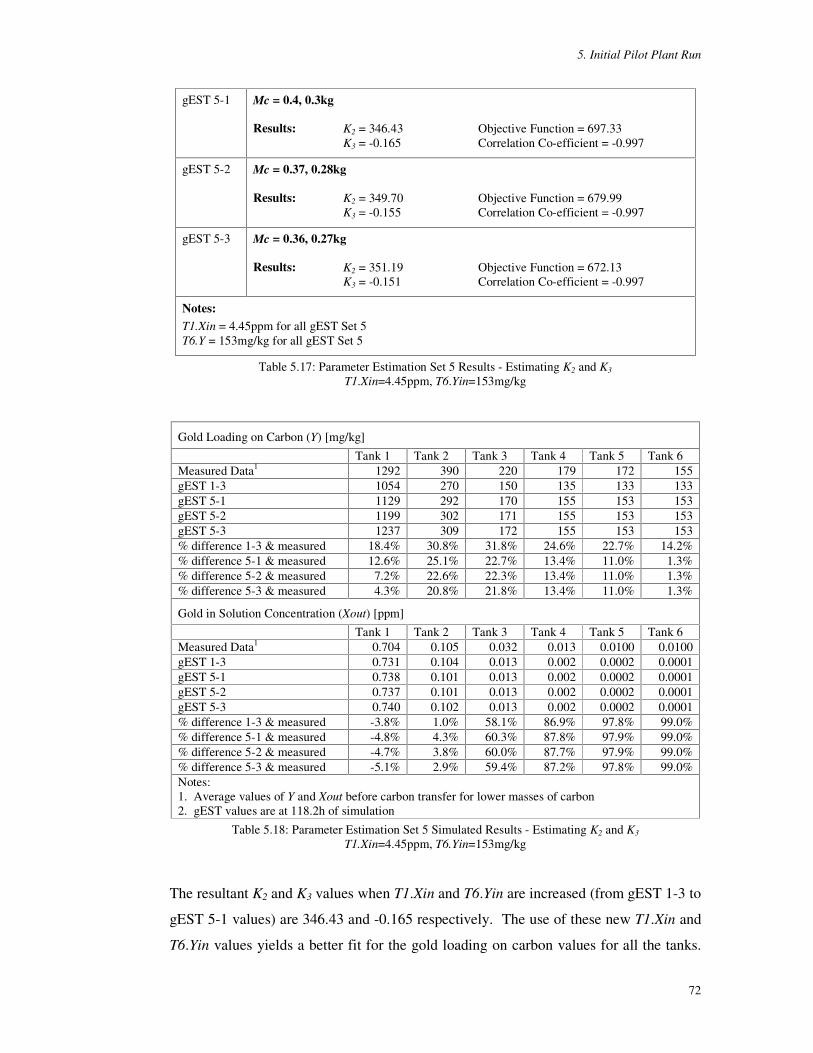
5. Initial Pilot Plant Run
72
gEST 5-1 Mc = 0.4, 0.3kg Results: K2 = 346.43 Objective Function = 697.33 K3 = -0.165 Correlation Co-efficient = -0.997
gEST 5-2 Mc = 0.37, 0.28kg Results: K2 = 349.70 Objective Function = 679.99 K3 = -0.155 Correlation Co-efficient = -0.997
gEST 5-3 Mc = 0.36, 0.27kg Results: K2 = 351.19 Objective Function = 672.13 K3 = -0.151 Correlation Co-efficient = -0.997
Notes: T1.Xin = 4.45ppm for all gEST Set 5 T6.Y = 153mg/kg for all gEST Set 5
Table 5.17: Parameter Estimation Set 5 Results - Estimating K2 and K3 T1.Xin=4.45ppm, T6.Yin=153mg/kg
Gold Loading on Carbon (Y) [mg/kg]
Tank 1 Tank 2 Tank 3 Tank 4 Tank 5 Tank 6 Measured Data1 1292 390 220 179 172 155 gEST 1-3 1054 270 150 135 133 133 gEST 5-1 1129 292 170 155 153 153 gEST 5-2 1199 302 171 155 153 153 gEST 5-3 1237 309 172 155 153 153 % difference 1-3 & measured 18.4% 30.8% 31.8% 24.6% 22.7% 14.2% % difference 5-1 & measured 12.6% 25.1% 22.7% 13.4% 11.0% 1.3% % difference 5-2 & measured 7.2% 22.6% 22.3% 13.4% 11.0% 1.3% % difference 5-3 & measured 4.3% 20.8% 21.8% 13.4% 11.0% 1.3%
Gold in Solution Concentration (Xout) [ppm] Tank 1 Tank 2 Tank 3 Tank 4 Tank 5 Tank 6 Measured Data1 0.704 0.105 0.032 0.013 0.0100 0.0100 gEST 1-3 0.731 0.104 0.013 0.002 0.0002 0.0001 gEST 5-1 0.738 0.101 0.013 0.002 0.0002 0.0001 gEST 5-2 0.737 0.101 0.013 0.002 0.0002 0.0001 gEST 5-3 0.740 0.102 0.013 0.002 0.0002 0.0001 % difference 1-3 & measured -3.8% 1.0% 58.1% 86.9% 97.8% 99.0% % difference 5-1 & measured -4.8% 4.3% 60.3% 87.8% 97.9% 99.0% % difference 5-2 & measured -4.7% 3.8% 60.0% 87.7% 97.9% 99.0% % difference 5-3 & measured -5.1% 2.9% 59.4% 87.2% 97.8% 99.0% Notes: 1. Average values of Y and Xout before carbon transfer for lower masses of carbon 2. gEST values are at 118.2h of simulation
Table 5.18: Parameter Estimation Set 5 Simulated Results - Estimating K2 and K3 T1.Xin=4.45ppm, T6.Yin=153mg/kg
The resultant K2 and K3 values when T1.Xin and T6.Yin are increased (from gEST 1-3 to
gEST 5-1 values) are 346.43 and -0.165 respectively. The use of these new T1.Xin and
T6.Yin values yields a better fit for the gold loading on carbon values for all the tanks.

5. Initial Pilot Plant Run
73
This is reflected in the lower objective function of 697 for gEST 5-1 compared with 715
for gEST 1-3.
As the masses of carbon are decreased from 0.4, 0.3kg (gEST 5-1) to the lower values
of 0.37, 0.28kg (gEST 5-2) and 0.36, 0.27kg (gEST 5-3), the resultant estimated K2 and
K3 values for gEST 5-2 and 5-3 are 354.70 and -0.155, and 351.19 and -0.151
respectively. The objective functions also decrease to 680 and 672 indicating a better fit
of the simulated data to the measured data as the masses of carbon are reduced. This is
reflected in the comparison of simulated and measured data in Table 5.18 where the
errors between the measured and simulated data for the gold loadings on carbon
decrease as the masses of carbon are decreased.
The initial error for the gold loading on carbon for Tank 1 (T1.Y) for gEST 1-3 was
18%. This decreased to 7.2% and 4.3% for gEST 5-2 and 5-3 respectively. The errors
for T2.Y and T3.Y decreased from 32% to 23%. The decrease in the error for the last 4
tanks is due to the higher T6.Yin value. The increase in the gold loading on carbon
values for Tanks 1 and 2 is also due to the increase in T6.Yin and T1.Xin, and the lower
carbon masses.
Changes in the masses of carbon, T6.Yin and T1.Xin have very little effect on the
simulated gold in solution concentration values. The gold in solution concentrations for
all the parameter estimations performed in this set are almost identical. In addition
when these values are compared with gEST 1-3 results, they too are very similar with
the simulated values of the parameter estimations within 0.01ppm of each other.
In conclusion, the best estimates of the actual masses of carbon used during the pilot
plant run are 0.36kg and 0.27kg. Using these masses, and combining them with the new
T1.Xin and T6.Yin values of 4.45ppm and 153mg/kg respectively, the most optimal
values of K2 and K3 determined in gEST 5-3, using gPROMS parameter estimation tool,
are 351.19 and -0.151 respectively. The graphs of the simulated and measured data for
the results of gEST 5-3 for all 6 tanks are shown in Figure 5.6 and the statistical data is
presented in the next section.

5. Initial Pilot Plant Run
74
0
500
1000
1500
2000
0 20 40 60 80 100 120
Time [h]
Tank
1G
old
on C
arbo
n [m
g/kg
]
0
200
400
600
800
1000
1200
0 20 40 60 80 100 120
Time [h]
Tank
2G
old
on C
arbo
n [m
g/kg
]
0
200
400
600
800
1000
0 20 40 60 80 100 120
Time [h]
Tank
3G
old
on C
arbo
n [m
g/kg
]
0
0.2
0.4
0.6
0.8
0 20 40 60 80 100 120
Time [h]
Tank
1G
old
in S
olut
ion
[ppm
]
0.00
0.10
0.20
0.30
0.40
0.50
0 20 40 60 80 100 120
Time [h]
Tank
2G
old
in S
olut
ion
[ppm
]
0.00
0.05
0.10
0.15
0.20
0 20 40 60 80 100 120
Time [h]
Tank
3G
old
in S
olut
ion
[ppm
]
0
200
400
600
800
0 20 40 60 80 100 120
Time [h]
Tan
k 4
Go
ld o
n C
arbo
n [m
g/k
g]
0
100
200
300
400
500
0 20 40 60 80 100 120
Time [h]
Tan
k 5
Gol
d o
n C
arbo
n [m
g/k
g]
0
50
100
150
200
250
0 20 40 60 80 100 120
Time [h]
Tan
k 6
Go
ld o
n C
arb
on [m
g/k
g]
0.00
0.01
0.02
0.03
0.04
0 20 40 60 80 100 120
Time [h]
Tan
k 4
Go
ld i
n S
olu
tion
[ppm
]
0.00
0.01
0.02
0.03
0.04
0 20 40 60 80 100 120
Time [h]
Tan
k 5
Gol
d in
Sol
utio
n [p
pm
]
0.00
0.01
0.02
0.03
0.04
0 20 40 60 80 100 120
Time [h]
Tan
k 6
Gol
d in
So
luti
on [p
pm]
Figure 5.6: gEST 5-3 - Gold loading on carbon and gold in solution concentration.
: Simulation, � Measured data.

5. Initial Pilot Plant Run
75
5.5 Statistical Analysis of Parameter Estimation
This section presents the statistical data from parameter estimation gEST 5-3. This
information is produced as part of the parameter estimation tool of gPROMS and is
presented in Table 5.19 and Figure 5.7. Table 5.19 shows the t-test values at 95%
significance for K2 and K3, and its 95% confidence intervals. The t-test reference value
at 95% significance is 1.654. This value is also calculated by the internal statistical
functions of gPROMS (Process Systems Enterprise, 2001).
The t-test values for K2 and K3 are 1.746 and 1.731 respectively and both are above the
critical value of 1.654. A t-value larger than the reference value indicates that the
corresponding parameter has been accurately estimated, hence the values of K2 and K3
are statistically significant. The 95% confidence intervals of K2 and K3 shown in Table
5.19, indicates that the value for K2 is not required to 5 significant values of accuracy as
previously stated and can be rounded to 350. The value of K3 will also be rounded to
-0.15. Hence the values of K2 and K3 that will be used are 350 and -0.15 respectively.
t-test values at 95% Reference Value 1.654 K2 1.746 K3 1.731
95% Confidence Intervals
K2 351.19 ± 201.11 K3 -0.151 ± 0.087
Table 5.19 Statistical data for gEST 5-3
Figure 5.7 shows the 95% joint confidence ellipsoid for K2 and K3. The plot shows an
elongated ellipsoid which is due to the very high correlation between the two parameter
values. The confidence interval intersects both axes at zero. This point is not a valid
solution for K2 and K3 even though it falls within the confidence interval.
High correlation between parameters can sometimes indicate that the model may be
over-parameterised. That is, one or more of the parameters may not be useful, or that a
re-parameterised model with fewer parameters may do just as well (Draper and Smith,
1981). The statistical data for this parameter estimation suggests this. However it must
also be noted that it does not mean that the original model is not appropriate for the

5. Initial Pilot Plant Run
76
system but may be an indication that the data used may not be enough or adequate for
the task of estimating the parameters (Draper and Smith, 1981).
95% Confidence Ellipsoid
-0.5
-0.4
-0.3
-0.2
-0.1
0
0.1
0.2
-400 -200 0 200 400 600 800 1000
K2
K3
Optimal point
Figure 5.7: 95% Confidence Ellipsoid for K2 and K3 for gEST 5-3
Hence, in conclusion, although the parameters are highly correlated, their 95% t-values
are higher than the reference value indicating their significance to the model. In
addition the values of the parameters determined by gEST 5-3 do provide an adequate
fit of plant data to simulated data. This is discussed in more detail in the next section.
5.6 Analysis of Simulation Results
The simulated results for the pilot plant run are the same as those for gEST 5-3
described in this chapter and are shown in Figure 5.6. Table 5.18 also shows the
simulated and actual data along with the percentage difference between the two values.
The results show that there is a good fit of simulated to actual data. For the gold
loadings on carbon, the percentage error is below 5% for Tank 1 and ranges between
11-22% for Tanks 2 to 5, and is 1% for Tank 6. For the gold in solution concentrations,
the fit for the first two tanks is very good with errors below 6%. However the errors are
very high for the final 4 tanks at over 59%. The extremely high percentage error is not
a true reflection of the actual error. Actual error values are very low for Tanks 3 to 6 at
less than 0.02ppm. In addition to this, there are large errors associated with the
detection of low gold in solution on the AAS and it is not uncommon to get errors in the
vicinity of 0.02ppm.
The gold mass balance calculation is performed to account for all the gold entering and
leaving the CIP pilot plant during the experimental run. It can also be used as a cross

5. Initial Pilot Plant Run
77
check for the adequacy of the sampling techniques used. That is, a large gold balance
error could indicate that the sampling procedures used may not be accurate. The gold
balance error is the error between the actual amount of gold entering the CIP system and
its calculated value.
The actual amount of gold entering the CIP pilot plant is determined from the amount of
gold feed solution entering the CIP pilot plant. The weight of the gold solution is
measured and used to determine the actual amount of gold entering the CIP pilot plant.
The calculated amount of gold entering the CIP pilot plant is determined from the
amount of gold removed from the CIP plant. This is calculated from the gold on carbon
recovered (i.e. the gold loading on the carbon removed from Tank 1 to elution), and the
gold loss to tailings. The gold losses to tailings include gold losses in solution and gold
losses in solids. In a real plant the gold losses in the solids are normally higher than
those in the solutions and this was also the case for the experimental runs. Gold losses
to solids in real plants are usually attributed to unleached gold in the ores or preg-
robbing ores. For the experimental runs, the gold losses in the tailings is due to gold
lost to carbon fines. The carbon fines are generated by abrasion of the carbon due to the
high speed of agitation required to keep the silica pulp in suspension.
The gold mass balance error for this experimental run is 2.1%. The calculation for this
is shown in Appendix E. The small error value confirms that the sampling techniques
used are satisfactory.
The simulated and measured results show the cyclical nature of the process. The
experimental results seem to indicate that the CIP pilot plant reaches a steady cyclical
state within 60 hours. This equates to approximately 2 time constants based on the
solution residence time in the entire CIP system. Given that the pilot plant was operated
on for a period of 5 days (120h), this means the plant ran for approximately 4 time
constants, which is long enough to establish a steady behaviour. Although the carbon
residence time is much longer at 3 days, the plant operated for a long enough time to
display its cyclical nature. The speed at which the CIP pilot plant reached steady
cyclical behaviour could be attributed to the perfect mixing of the tanks, adequate
carbon cycle times and pulp flowrate.
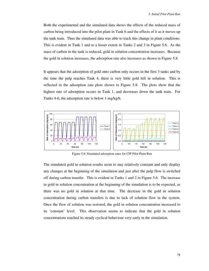
5. Initial Pilot Plant Run
78
Both the experimental and the simulated data shows the effects of the reduced mass of
carbon being introduced into the pilot plant in Tank 6 and the effects of it as it moves up
the tank train. Thus the simulated data was able to track this change in plant conditions.
This is evident in Tank 1 and to a lesser extent in Tanks 2 and 3 in Figure 5.6. As the
mass of carbon in the tank is reduced, gold in solution concentration increases. Because
the gold in solution increases, the adsorption rate also increases as shown in Figure 5.8.
It appears that the adsorption of gold onto carbon only occurs in the first 3 tanks and by
the time the pulp reaches Tank 4, there is very little gold left in solution. This is
reflected in the adsorption rate plots shown in Figure 5.8. The plots show that the
highest rate of adsorption occurs in Tank 1, and decreases down the tank train. For
Tanks 4-6, the adsorption rate is below 1 mg/kg/h.
0
20
40
60
80
100
0 20 40 60 80 100 120
Time [h]
Rat
e o
f A
dso
rpti
on [
mg/
kg/h
]
Tank 1
Tank 2
0.0
0.5
1.0
1.5
2.0
2.5
0 20 40 60 80 100 120
Time [h]
Rat
e o
f A
dso
rpti
on [
mg/
kg/h
]
Tank 3
Tank 4
Tank 5
Tank 6
Figure 5.8: Simulated adsorption rates for CIP Pilot Plant Run
The simulated gold in solution results seem to stay relatively constant and only display
any changes at the beginning of the simulation and just after the pulp flow is switched
off during carbon transfer. This is evident in Tanks 1 and 2 in Figure 5.6. The increase
in gold in solution concentration at the beginning of the simulation is to be expected, as
there was no gold in solution at that time. The decrease in the gold in solution
concentration during carbon transfers is due to lack of solution flow in the system.
Once the flow of solution was restored, the gold in solution concentration increased to
its ‘constant’ level. This observation seems to indicate that the gold in solution
concentrations reached its steady cyclical behaviour very early in the simulation.
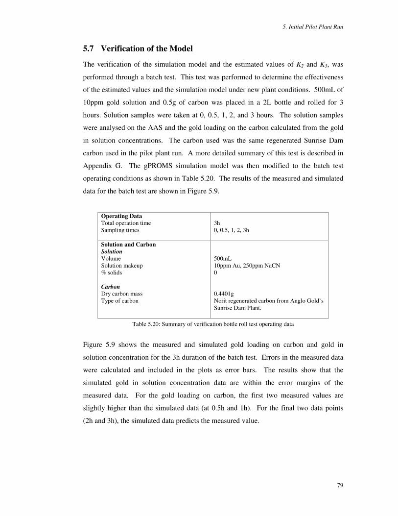
5. Initial Pilot Plant Run
79
5.7 Verification of the Model
The verification of the simulation model and the estimated values of K2 and K3, was
performed through a batch test. This test was performed to determine the effectiveness
of the estimated values and the simulation model under new plant conditions. 500mL of
10ppm gold solution and 0.5g of carbon was placed in a 2L bottle and rolled for 3
hours. Solution samples were taken at 0, 0.5, 1, 2, and 3 hours. The solution samples
were analysed on the AAS and the gold loading on the carbon calculated from the gold
in solution concentrations. The carbon used was the same regenerated Sunrise Dam
carbon used in the pilot plant run. A more detailed summary of this test is described in
Appendix G. The gPROMS simulation model was then modified to the batch test
operating conditions as shown in Table 5.20. The results of the measured and simulated
data for the batch test are shown in Figure 5.9.
Operating Data Total operation time Sampling times
3h 0, 0.5, 1, 2, 3h
Solution and Carbon Solution Volume Solution makeup % solids Carbon Dry carbon mass Type of carbon
500mL 10ppm Au, 250ppm NaCN 0 0.4401g Norit regenerated carbon from Anglo Gold’ s Sunrise Dam Plant.
Table 5.20: Summary of verification bottle roll test operating data
Figure 5.9 shows the measured and simulated gold loading on carbon and gold in
solution concentration for the 3h duration of the batch test. Errors in the measured data
were calculated and included in the plots as error bars. The results show that the
simulated gold in solution concentration data are within the error margins of the
measured data. For the gold loading on carbon, the first two measured values are
slightly higher than the simulated data (at 0.5h and 1h). For the final two data points
(2h and 3h), the simulated data predicts the measured value.

5. Initial Pilot Plant Run
80
0
500
1000
1500
2000
2500
3000
3500
0 1 2 3
Time [h]
Gol
d Lo
adin
g on
Car
bon
[mg/
kg]
Measured Simulation
7.0
7.5
8.0
8.5
9.0
9.5
10.0
0 1 2 3
Time [h]
Gol
d in
Sol
utio
n C
once
ntra
tion
[ppm
]
Measured Simulation
Figure 5.9: Plot of results of the batch test to verify the simulation model
An analysis of the percentage errors between the measured and simulated data of the
batch test, shown in Table 5.21, confirms the satisfactory fit of the gold in solution
values with errors of less than 2%. Errors in the gold loading on carbon values are
higher, especially for the first data point at 18.5% (0.5h). For the other three data
points, it is 6% or less. Even though the error is high for the 0.5h data, the simulated
gold loading on carbon does predict the trend and is within 6% of the measured values
for three of the four data points.
In conclusion, the results show that the simulation model and the estimated values of K2
and K3 are able to predict the behaviour of gold adsorption onto activated carbon.
Gold Loading on Carbon (Y) [mg/kg] Time [h] 0.5 1 2 3 Measured Data 880 1358 2305 2873 Simulated Data 717 1277 2226 3030 % difference 18.51% 5.97% 3.44% -5.45%
Gold in Solution Concentration (X) [ppm]
Time [h] 0.5 1 2 3 Measured Data 9.08 8.65 7.80 7.29 Simulated Data 9.23 8.72 7.87 7.15 % difference -1.61% -0.84% -0.91% 1.93%
Table 5.21: Results of model verification batch test

5. Initial Pilot Plant Run
81
5.8 Conclusion
In conclusion, five sets of parameter estimations were performed to determine the best
combination of adsorption parameters, K2 and K3. The first set of parameter estimations
were performed to determine the best combination of weightings to be used for the
parameter estimations as well as the first estimate of K2 and K3. The fit of the gold in
solution simulated data to its measured values was satisfactory. However for the gold
loading on carbon, the simulated data consistently under-predicted the measured values.
The next four parameter estimations were performed to overcome this under-prediction.
Investigations were carried out on some of the input values used in the simulation
model. This resulted in a new value for the gold in solution concentration entering Tank
1, of 4.45pmm, a new value for the gold loading on the carbon entering the system in
Tank 6, of 153mg/kg and new masses of carbon values of 0.36, 0.27kg. These values
were used in the final set of parameter estimations and the resultant K2 and K3 values
were 350 and -0.15 respectively.
An analysis of the fit of the simulated model to the experimental data shows that the
model data provides a good fit to the experimental data. The simulation also shows the
cyclical nature of the adsorption process and was able to display the dynamic changes of
the system when the mass of the carbon into the system was reduced.
The results of the independent batch test shows that the model was able to predict the
measured data. Hence the simulation model has been successfully verified. The next
chapter will perform sensitivity analyses on different parameters and variables of the
model to determine their influence on the model. The model can then be used to
optimise the operations of the pilot plant and to investigate different carbon
management strategies detailed in Chapter 7.

82
6. Sensitivity Analysis
A series of sensitivity analyses are performed on selected variables and
parameters of the CIP simulation model to determine their influence on the
model.
6.1 Introduction
This chapter will detail the sensitivity analyses performed on selected variables and
parameters of the CIP simulation model to determine whether they have a significant
effect on the model, and hence will require careful estimation. The parameters and
variables chosen are the four model parameters A, b, K2 and K3, the amount of gold
entering the system into Tank 1 (T1.Xin) and the mass of carbon in each tank (Mc).
6.2 Simulation Conditions
The simulation operating conditions for these sensitivity simulations are the same as
those used to determine the operating point of the CIP pilot plant described in Section
7.3.1 and are summarised in Table 7.8. Note that these conditions are different to those
used previously, but are considered appropriate in view of the conditions that the pilot
plant will be subjected to in subsequent work. The main difference is the pulp flowrate,
which is set to 18L/h for the sensitivity analysis and was 8.18L/h for the previous
chapter. This higher flowrate was chosen such that plant response to changes in plant
conditions would be more sensitive. The details of how this flowrate of 18L/h was
chosen are in Section 7.3.1.
The CIP plant consisted of six 40L tanks. The plant was simulated at 12h carbon
cycles, for 24 cycles, for a total of 288h. The pulp consisted of 40% silica flour, at a
flowrate of 18L/h with a gold in solution concentration of 4.45ppm. The carbon content
in each of the CIP tanks was 4g/L which equated to 0.16kg of carbon in each tank.
During carbon transfer, 60% (0.096kg) of the total amount of carbon in each tank was
transferred. The initial carbon gold loading was set to 1mg/kg and all new carbon put
into the plant was of this loading value. The initial gold in solution concentration for all

6. Sensitivity Analysis
83
tanks was 0ppm. Gold loading on carbon and gold in solution concentrations for all 6
tanks were recorded for the last cycle of the simulation and used for the sensitivity
analyses.
Sensitivity simulations were performed for ±5%, 10%, 20% and 50% of the original
values of A, b, K2 and K3, and T1.Xin. Table 6.1 lists the values of the parameters for
each sensitivity simulation. For the analysis of the mass of carbon, simulations were
performed for a carbon content ranging from 2g/L (0.08kg) to 16g/L (0.64kg). A total
of 60 sensitivity simulations were performed. Nine simulations were performed for
each of the sensitivity analyses on A, b, K2 and K3, and T1.Xin, and 15 simulations were
performed on the mass of carbon.
Fraction of original value
A b K2 K3 T1.Xin
0.50 3733 0.170 175 -0.075 2.225 0.80 5973 0.272 280 -0.120 3.560 0.90 6719 0.306 315 -0.135 4.005 0.95 7093 0.323 333 -0.143 4.228 1.00 7466 0.340 350 -0.150 4.450 1.05 7839 0.357 368 -0.158 4.673 1.10 8213 0.374 385 -0.165 4.895 1.20 8959 0.408 420 -0.180 5.340 1.50 11199 0.510 525 -0.225 6.675
Table 6.1: Summary of the values of A, b, K2, K3 and T1.Xin for the sensitivity analysis simulations
6.3 Simulation Results
The results of the sensitivity analysis for each parameter or variable are presented
separately. For each simulation, data on the gold loadings on carbon and gold in
solution concentrations at the point before the last carbon transfer of the simulation
were collected. A select few will be presented in this chapter and the complete set of
the results of the gold loading on carbon and gold in solution values for all tanks are
shown in Appendix H. The results of the sensitivity analysis of the Freundlich Isotherm
parameters A and b are presented first, followed by the adsorption rate model
parameters K2 and K3, then the gold in solution concentration entering the CIP plant
(T1.Xin) and finally the masses of carbon in each tank.

6. Sensitivity Analysis
84
6.3.1 Freundlich Isotherm A
The results of the sensitivity analysis simulations of Freundlich Isotherm parameter A
are shown in Figure 6.1 to Figure 6.3. These figures show the gold loading on carbon
leaving Tanks 1 and 2 (T1.Y, T2.Y), and the gold in solution in Tank 6 (T6.Xout) for
different fractions of A from 0.5 to 1.5. The gold loading on carbon for Tank 1 and the
gold in solution concentration for Tank 6 are the most important values to the CIP
process, as they allow the calculation of the amount of gold removed from the CIP plant
and the gold losses to tailings. Only the results for T1.Y, T2.Y and T6.Xout are shown to
illustrate the sensitivity of A, the remaining results are shown in Appendix H.
The results show that as A increases, the gold loading on carbon in Tank 1 increases,
and the gold loading for Tanks 2 to 6, and the gold in solution concentration for all
tanks decreases. This is more apparent for the gold loading on carbon for Tank 1 and
gold in solution concentration for Tank 6 in Figure 6.2, where the smallest fraction of
0.5 is not shown and the results are plotted for fractions of A from 0.8 to 1.5. This
behaviour can be explained by the form of the model equations and the counter-current
movement of the carbon. Firstly, recall from Chapter 3, the adsorption rate and the
isotherm equations which are reproduced below in Equation (6.1) and (6.2).
Xe)(XoutYKR K −= 32 (6.1)
b
AY
Xe1
=
(6.2)
where R is the rate of gold adsorbed on to carbon [mg/kg/h], Y is the gold loading on
carbon [mg/kg], Xout is the gold in solution concentration [ppm], Xe is the equilibrium
gold in solution concentration [ppm], K2 and K3 are the adsorption rate constants and A
and b are the isotherm parameters. Given the above equations, if there is an increase in
A for Tank 1, then the equilibrium value Xe will decrease. A smaller Xe will result in an
increase in the rate of adsorption of gold onto carbon and hence, increase the gold
loading on carbon in Tank 1. If more of the incoming gold in solution into the CIP
plant (i.e. Tank 1) is being adsorbed (due to the increase in A), then the amount of gold
in solution in all the tanks will decrease. The different behaviour of gold loading on
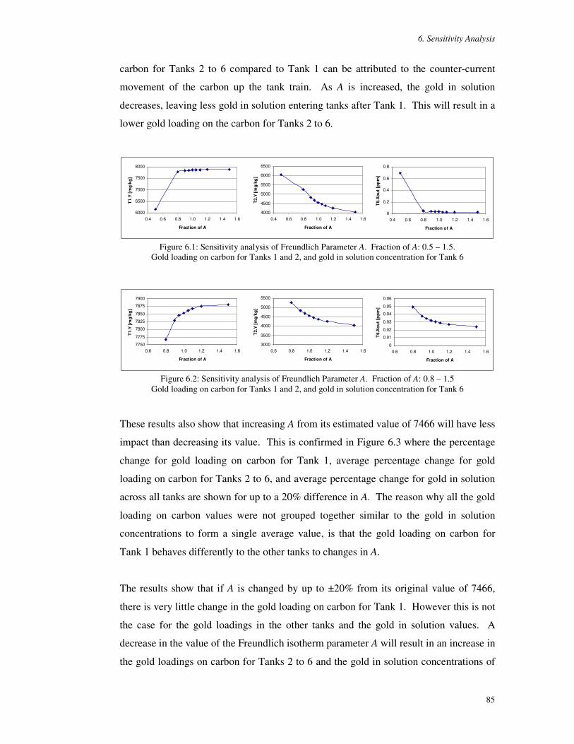
6. Sensitivity Analysis
85
carbon for Tanks 2 to 6 compared to Tank 1 can be attributed to the counter-current
movement of the carbon up the tank train. As A is increased, the gold in solution
decreases, leaving less gold in solution entering tanks after Tank 1. This will result in a
lower gold loading on the carbon for Tanks 2 to 6.
6000
6500
7000
7500
8000
0.4 0.6 0.8 1.0 1.2 1.4 1.6
Fraction of A
T1.
Y [
mg
/kg]
0
0.2
0.4
0.6
0.8
0.4 0.6 0.8 1.0 1.2 1.4 1.6
Fraction of A
T6.
Xou
t [p
pm
]
4000
4500
5000
5500
6000
6500
0.4 0.6 0.8 1.0 1.2 1.4 1.6
Fraction of A
T2.Y
[mg/
kg]
Figure 6.1: Sensitivity analysis of Freundlich Parameter A. Fraction of A: 0.5 – 1.5.
Gold loading on carbon for Tanks 1 and 2, and gold in solution concentration for Tank 6
7750
7775
7800
7825
7850
7875
7900
0.6 0.8 1.0 1.2 1.4 1.6
Fraction of A
T1.Y
[mg/
kg]
0
0.01
0.02
0.03
0.04
0.05
0.06
0.6 0.8 1.0 1.2 1.4 1.6
Fraction of A
T6.
Xo
ut [
ppm
]
3000
3500
4000
4500
5000
5500
0.6 0.8 1.0 1.2 1.4 1.6
Fraction of A
T2.
Y [m
g/k
g]
Figure 6.2: Sensitivity analysis of Freundlich Parameter A. Fraction of A: 0.8 – 1.5
Gold loading on carbon for Tanks 1 and 2, and gold in solution concentration for Tank 6
These results also show that increasing A from its estimated value of 7466 will have less
impact than decreasing its value. This is confirmed in Figure 6.3 where the percentage
change for gold loading on carbon for Tank 1, average percentage change for gold
loading on carbon for Tanks 2 to 6, and average percentage change for gold in solution
across all tanks are shown for up to a 20% difference in A. The reason why all the gold
loading on carbon values were not grouped together similar to the gold in solution
concentrations to form a single average value, is that the gold loading on carbon for
Tank 1 behaves differently to the other tanks to changes in A.
The results show that if A is changed by up to ±20% from its original value of 7466,
there is very little change in the gold loading on carbon for Tank 1. However this is not
the case for the gold loadings in the other tanks and the gold in solution values. A
decrease in the value of the Freundlich isotherm parameter A will result in an increase in
the gold loadings on carbon for Tanks 2 to 6 and the gold in solution concentrations of

6. Sensitivity Analysis
86
similar percentage change or greater. That is, if A is decreased by 5%, 10% or 20%,
then the gold loadings on carbon for Tanks 2 to 6 and the gold in solution
concentrations increases by approximately 5%, 10% or 30% respectively. If A is
increased by a certain percentage, the decrease in gold loadings on carbon for Tanks 2
to 6 and the gold in solution concentrations is less than that percentage as shown in
Figure 6.3.
-20%
-10%
0%
10%
20%
30%
40%
50%
0.7 0.8 0.9 1.0 1.1 1.2 1.3
Fraction of A
% c
hang
e fr
omFr
actio
n =1
val
ue
T1.Y T2 to 6.Y Xout
Figure 6.3: Sensitivity analysis of Freundlich Parameter A. %change in gold loading on carbon and gold in solution concentration with changes in A.
Another observation in these results is the magnitude of the gold loading on carbon in
Tank 1 (T1.Y) and the gold in solution concentration of Tank 6 (T6.Xout), or gold lost to
tailings. As stated earlier, these two values are the most important in the CIP process.
T1.Y determines the amount of gold removed from the CIP process to elution and hence
the revenue generated by the plant, and T6.Xout determines the amount of gold loss to
tailings. Hence operating conditions are chosen to maximise gold revenue (T1.Xout)
and minimise gold losses (T6.Xout).
The results show that changes in A up to ±20% will have a small effect on T1.Y. The
effect on T6.Xout is greater. However it must be noted that the gold losses to tailings
for ±20% changes in the isotherm parameter A ranges from 0.025-0.05ppm. This is
within the reported range of 0.002-0.05ppm of gold in solution concentration to tailings
in surveyed gold plants in Australia (Barbetti et al, 2000). The 0.05ppm value will be
used as the maximum acceptable gold loss to tailings value in this work.
In summary the CIP pilot plant is sensitive to changes in the estimated value of the
Freundlich isotherm parameter A, especially the gold loadings on carbon for Tanks 2 to

6. Sensitivity Analysis
87
6 and the gold in solution concentrations. However it must be noted that the
performance of the CIP plant is not sensitive to variations in the parameter above 0.8 of
the currently estimated value.
6.3.2 Freundlich Isotherm b
The results of the sensitivity of Freundlich isotherm parameter b on the simulation
model are shown in Figure 6.4 and Figure 6.5. The results show that as b increases,
there is a slight decrease in gold loading on carbon for Tank 1 and gold in solution
concentration for Tank 1, and the gold loading on carbon and the gold in solution
concentrations for Tanks 2 to 6 increase. As the gold loading on carbon in Tank 1
decreases with increasing b, there is a corresponding small decrease in the gold in
solution concentration for Tank 1. This leaves more gold in solution to flow down the
CIP train to the other tanks, increasing the gold in solution concentrations for all the
tanks, and increasing the gold loadings on carbon for Tanks 2 to 6.
7800
7820
7840
7860
7880
7900
0.4 0.6 0.8 1.0 1.2 1.4 1.6
Fraction of b
T1.
Y [m
g/k
g]
0
0.01
0.02
0.03
0.04
0.05
0.4 0.6 0.8 1.0 1.2 1.4 1.6
Fraction of b
T6.
Xo
ut [p
pm
]
4400
4450
4500
4550
4600
4650
0.4 0.6 0.8 1.0 1.2 1.4 1.6
Fraction of b
T2.
Y [
mg/
kg]
2.5
2.6
2.7
2.8
2.9
3.0
0.4 0.6 0.8 1.0 1.2 1.4 1.6
Fraction of b
T1.
Xo
ut
[pp
m]
Figure 6.4: Sensitivity analysis of Freundlich Parameter b. Fraction of b: 0.5 – 1.5.
Gold loading on carbon for Tanks 1 and 2, and gold in solution concentration for Tanks 1 and 6
This behaviour is the opposite of previous sensitivity analysis on isotherm parameter A,
but has lesser impact. For example, the magnitude of change in the gold loading on
carbon for Tank 1 from 0.5 to 1.5 fractions of A is approximately 1700mg/kg, compared
with 20mg/kg for b, and for gold in solution to tailings, the difference in value from 0.5
to 1.5 fractions of A is 0.7ppm compared to 0.01ppm for b. These observations are
confirmed in Figure 6.5, which shows the percentage changes in the gold loadings on

6. Sensitivity Analysis
88
carbon and gold in solution concentrations for changes in b up to ±20%. The plot
shows that changes in b up to ±20% will result in less than a 1% change in the gold
loading on carbon for Tank 1, and approximately 5% change for gold loading on carbon
for Tanks 2 to 6 and gold in solutions for all tanks. In summary, gold loading on carbon
and gold in solution concentration for the CIP plant is not sensitive to changes in the
currently estimated value Freundlich isotherm parameter b.
-6%
-4%
-2%
0%
2%
4%
6%
0.7 0.8 0.9 1.0 1.1 1.2 1.3
Fraction of b
% c
hang
e fr
omFr
actio
n =1
val
ue
T1.Y T2 to 6.Y Xout
Figure 6.5: Sensitivity analysis of Freundlich Parameter b. %change in gold loading on carbon and gold in solution concentration with changes in b.
6.3.3 Adsorption Parameter K2
The results of the sensitivity analysis for adsorption parameter K2 are shown in Figure
6.6 and Figure 6.7. The results show that as the adsorption parameter K2 increases, the
gold loading on carbon for Tank 1 increases, and the gold loading on carbon in Tanks 2
to 6 and the gold in solution concentrations for all tanks decreases. These results are
similar to those of the sensitivity analysis on Freundlich isotherm parameter A, but have
less impact. That is, the magnitude of the changes in gold loading on carbon and gold
in solution concentration values are less for K2 but larger than for the Freundlich
isotherm parameter b.
7000
7200
7400
7600
7800
8000
0.4 0.6 0.8 1.0 1.2 1.4 1.6
Fraction of K2
T1.Y
[mg/
kg]
0.00
0.05
0.10
0.15
0.20
0.25
0.30
0.4 0.6 0.8 1.0 1.2 1.4 1.6
Fraction of K2
T6.
Xo
ut [
ppm
]
3000
3500
4000
4500
5000
5500
0.4 0.6 0.8 1.0 1.2 1.4 1.6
Fraction of K2
T2.
Y [m
g/k
g]
Figure 6.6 Sensitivity analysis of Adsorption Parameter K2. Fraction of K2: 0.5 – 1.5.
Gold loading on carbon for Tanks 1 and 2, and gold in solution concentration for Tank 6

6. Sensitivity Analysis
89
An increase in K2 in Equation (6.1), assuming all other values remain the same, would
result in an increase in the rate of adsorption. However, as this system is for 6 tanks and
the tanks are connected in series, the effect of an increase in K2 is more complex. An
increase in K2 results in an increase in gold loading on carbon in Tank 1. When this
occurs, the gold in solution concentration decreases for all tanks. As there is a decrease
in gold in solution, then there is less gold in solution to adsorb onto the carbon, hence
there is a decrease in the gold loadings on carbon for Tanks 2 to 6.
Figure 6.6 also shows a decrease in K2 below 0.9 of the currently estimated value will
result in a predicted gold loss to tailings of greater that 0.05ppm. Hence if the true
value of K2 is below 90% of its original value of 350, it will have an adverse affect on
the operations of the CIP plant.
Figure 6.7 shows the percentage change in gold loadings on carbon and gold in solution
concentrations with changes in K2 of up to ±20%. The results show that decreasing K2
has a larger effect on gold loadings on carbon and gold in solution concentrations than
increasing K2. This is similar to the results of isotherm parameter A. The results also
show that changing K2 in the range of 0.8 to 1.5 of K2 will result in very little change in
gold loading on carbon for Tank 1, and will change the gold loading on carbon for
Tanks 2 to 6 and the gold in solution concentrations by a similar percentage or more. In
summary, changes in K2 do have an effect on the predicted CIP plant performance.
-40%
-20%
0%
20%
40%
60%
0.7 0.8 0.9 1.0 1.1 1.2 1.3
Fraction of K2
% c
hang
e fr
om
Frac
tion
=1 v
alue
T1.Y T2 to 6.Y Xout
Figure 6.7 Sensitivity analysis of Adsorption Parameter K2. %change in gold loading on carbon and gold in solution concentration with changes in K2.

6. Sensitivity Analysis
90
6.3.4 Adsorption Parameter K3
The results of the sensitivity analysis for adsorption parameter K3 are shown in Figure
6.8 and Figure 6.9. The results are almost a mirror image of the adsorption parameter
K2 results, where the gold loading on carbon for Tank 1 decreases with increasing K3,
and the gold loading on carbon for Tanks 2 to 6 and the gold in solution concentration
increases with increasing K3.
The reason for this behaviour is the opposite of that described for K2. That is, as K3
increases, a decrease in gold loading on Tank 1 occurs. If the gold loading in Tank 1
decreases, then the gold in solution concentrations for all tanks will increase. This will
then result in an increase in the gold loadings on the carbon for Tanks 2 to 6.
Figure 6.8 also shows that the gold lost to tailings is above 0.05ppm at fractions of K3
above 1.1. Hence if the true value of K3 is above this fraction of 1.1, it will have an
adverse effect on the operations of the CIP plant by increasing gold losses to tailings
above the limiting value of 0.05ppm.
7000
7200
7400
7600
7800
8000
0.4 0.6 0.8 1.0 1.2 1.4 1.6
Fraction of K3
T1.
Y [
mg
/kg]
0.00
0.05
0.10
0.15
0.20
0.25
0.4 0.6 0.8 1.0 1.2 1.4 1.6
Fraction of K3
T6.
Xou
t [p
pm
]
3000
3500
4000
4500
5000
5500
0.4 0.6 0.8 1.0 1.2 1.4 1.6
Fraction of K3
T2.Y
[mg/
kg]
Figure 6.8: Sensitivity analysis of Adsorption Parameter K3. Fraction of K3: 0.5 – 1.5.
Gold loading on carbon for Tanks 1 and 2, and gold in solution concentration for Tank 6
An analysis of the percentage change in gold loadings on carbon and gold in solution
with changes in K3 is shown in Figure 6.9. This plot again shows there is little
significant change in gold loadings on carbon for Tank 1 with changes in K3. However
this is not the case for the gold loadings on carbon for the other tanks and the gold in
solution concentrations. The plot also shows that the magnitude of change is greater
when K3 is increased. For example a 20% increase in K3 will result in a 60% increase in
the gold loading on carbon for Tanks 2 to 6 and a 40% increase in gold in solution
concentrations. A 20% decrease in K3 will result in a 30% decrease in the gold loading
on carbon for Tanks 2 to 6 and the gold in solution concentrations. Therefore the CIP
plant is sensitive to changes in adsorption parameter K3.

6. Sensitivity Analysis
91
-40%
-20%
0%
20%
40%
60%
0.7 0.8 0.9 1.0 1.1 1.2 1.3
Fraction of K3
% c
hang
e fr
om
Frac
tion
=1 v
alue
T1.Y T2 to 6.Y Xout
Figure 6.9: Sensitivity analysis of Adsorption Parameter K3. %change in gold loading on carbon and gold in solution concentration with changes in K3.
6.3.5 Gold in Solution Concentration Entering the CIP Plant
The results of the sensitivity analysis of the gold in solution concentration entering the
CIP plant (T1.Xin) are shown in Figure 6.10 and Figure 6.11. The results show that as
T1.Xin increases, the gold loading on the carbon and the gold in solution concentrations
for all tanks increase. Figure 6.10 shows the critical fraction of T1.Xin to minimise gold
losses to below 0.05ppm is 1.2 for the plant operating conditions used for the sensitivity
analyses. Fractions of T1.Xin above this value will result in high gold losses to tailings,
adversely affecting the performance of the CIP plant.
0
3000
6000
9000
12000
15000
0.4 0.6 0.8 1.0 1.2 1.4 1.6
Fraction of T1.Xin
T1.Y
[mg/
kg]
0.00
0.03
0.06
0.09
0.12
0.4 0.6 0.8 1.0 1.2 1.4 1.6
Fraction of T1.Xin
T6.
Xo
ut [
ppm
]
0
2000
4000
6000
8000
10000
0.4 0.6 0.8 1.0 1.2 1.4 1.6
Fraction of T1.Xin
T2.
Y [m
g/k
g]
Figure 6.10: Sensitivity analysis of T1.Xin. Fraction of T1.Xin: 0.5 – 1.5.
Gold loading on carbon for Tanks 1 and 2, and gold in solution concentration for Tank 6
Figure 6.11 shows the percentage change in gold loading on carbon and gold in solution
concentration with changes in T1.Xin. The plot shows that there is a positive linear
relationship between the percentage change in gold loading on the carbon for Tank 1
and T1.Xin. That is, if T1.Xin is increased or decreased by a certain percentage, then the
gold loading on carbon for Tank 1 will also change by the same percentage. The effect
of changes in T1.Xin on the gold loading on carbon for Tanks 2 to 6 and the gold in
solution concentration is greater, as shown in Figure 6.11. Hence the amount of gold

6. Sensitivity Analysis
92
entering the CIP plant will have a significant effect on the gold loading on carbon and
the gold in solution concentration for all tanks.
-40%
-20%
0%
20%
40%
60%
0.7 0.8 0.9 1.0 1.1 1.2 1.3
Fraction of A
% c
hang
e fr
omFr
actio
n =1
val
ue
T1.Y T2 to 6.Y Xout
Figure 6.11: Sensitivity analysis of T1.Xin. %change in gold loading on carbon and gold in solution concentration with changes in T1.Xin
6.3.6 Mass of Carbon
The final sensitivity analysis performed was to determine the effect of changes in
masses of carbon – or carbon content [g/L] on the CIP system.
The results of the sensitivity of the carbon content on the CIP plant are shown in Figure
6.12 and Figure 6.13. The results show the plots of gold loading on carbon and gold in
solution concentrations for carbon content of 2 to 16g/L. The results show that as the
carbon content is increased, the gold loading on carbon and the gold in solution
concentration decreases. The increase in carbon content in the tanks redistributes the
gold in solution to a greater amount of carbon and hence there is a decrease in the gold
loadings on the carbon. The increased amount of carbon reduces the amount of gold in
solution to very low values as illustrated in Figure 6.13. This plot shows the gold in
solution concentration for Tank 6 from a carbon content of 4 to 16g/L. The gold in
solution concentration for Tank 6 starts at 1ppm for a carbon content of 2g/L (see
Figure 6.12) and then decreases dramatically to 0.03ppm at only 4g/L (see Figure 6.13).
For carbon content of 5g/L and above, T6.Xout is at 0.01ppm or less. As it is difficult to
detect gold in solution a concentrations below 0.01ppm, these results suggest that a
carbon content of greater that 5g/L will not be of benefit to the CIP system. This is
confirmed in Figure 6.14 which shows a plot of the total amount of gold removed from
Tank 1, and the amount of gold lost to tailings in [mg] of gold. Both are plotted against
carbon content ranging from 2 to 16g/L.

6. Sensitivity Analysis
93
0
3000
6000
9000
12000
15000
0 2 4 6 8 10 12 14 16
Carbon Content [g/L]T1
.Y [m
g/kg
]
0.0
0.3
0.6
0.9
1.2
0 2 4 6 8 10 12 14 16
Carbon Content [g/L]
T6.
Xo
ut [
ppm
]
0
3000
6000
9000
12000
0 2 4 6 8 10 12 14 16
Carbon Content [g/L]
T2.
Y [m
g/k
g]
Figure 6.12: Sensitivity analysis of carbon mass. Carbon content: 2 – 16g/L.
Gold loading on carbon for Tanks 1 and 2, and gold in solution concentration for Tank 6
0.00
0.01
0.02
0.03
0.04
0 2 4 6 8 10 12 14 16
Carbon Content [g/L]
T6.
Xou
t [pp
m]
Figure 6.13: Sensitivity analysis of carbon mass.
Gold in solution concentration for Tank 6 for carbon content of 4 – 16g/L
Figure 6.14 shows the amount of gold removed from the CIP system from Tank 1
increases as the carbon content increases from 2g/L to 5g/L and then plateaus. A
similar behaviour is observed for the gold losses to tailings where it is very high at
170mg of gold for a carbon content of 2g/L and drops dramatically to almost zero at
5g/L. The results show that there exists an optimal carbon content for certain operating
conditions of a CIP process. For this case the optimal carbon content is between 4 and
5g/L. This is investigated further in Section 7.3.2.
500
550
600
650
700
750
800
0 2 4 6 8 10 12 14 16
Carbon Content [g/L]
Go
ld o
n C
arb
on
[mg
]
0
30
60
90
120
150
180
Go
ld lo
ss [
mg
]
Gold on Carbon Gold loss to tailings
Figure 6.14: Sensitivity analysis of carbon mass.
Gold in solution concentration for Tank 6 for carbon content of 4 – 16g/L

6. Sensitivity Analysis
94
6.4 Conclusion
Six sensitivity analyses were performed on the Freundlich isotherm parameters A and b,
adsorption rate parameters K2 and K3, gold in solution concentration entering the CIP
system (T1.Xin) and the carbon content in the tanks. It was found that gold loading on
carbon and gold in solution concentrations for all tanks were not sensitive to changes in
the Freundlich isotherm parameter b. Changes in the Freundlich isotherm parameter A,
and adsorption rate parameters K2 and K3, had little effect on the gold loading on carbon
for Tank 1, but did effect the gold loading on carbon for Tanks 2 to 6 and the gold in
solution concentrations for all tanks. Changes in both T1.Xin and carbon content have a
significant effect on gold loading on carbon and gold in solution concentration for all
tanks. Hence, the parameters and variables that do require careful estimation are the
Freundlich isotherm parameter A, the adsorption rate parameters K2 and K3, the gold in
solution concentration entering the CIP system, and the carbon content in the tanks.

95
7. Optimisation of Carbon in Pulp Process
An objective function of the CIP process is developed. The operations of the
CIP pilot plant is optimised. Different carbon management strategies are
investigated. The proposal of recirculating a portion of the tailing pulp back
into the CIP process and adding fresh carbon into the CIP system in other
tanks as well as the last tank are investigated.
7.1 Introduction
In this chapter, the simulation model developed in Chapter 3 was used to optimise the
performance of a CIP pilot plant by performing a series of simulations under different
operating conditions. The most optimal operating condition was determined through
evaluating values of an objective function. The simulation model along with the
objective function developed was used to investigate different carbon management
strategies.
This chapter is organised as follows. Firstly the objective function of the CIP model is
detailed in Section 7.2. Then the operations of the CIP pilot plant are optimised in
Section 7.3. The investigation of the different carbon management strategies are
detailed in Section 7.4 and 7.5, and finally conclusions are presented in Section 7.6.
7.2 Objective Function Equations
An objective function was developed to quantitatively compare different carbon
management strategies and to optimise the CIP pilot plant process. The objective
function is based on the gold revenue of the CIP process, the capital and operational
costs, and the gold losses to tailings. Kiranoudis et al (1998) also investigated different
carbon management strategies based on economic evaluation of the CIP process.
Kiranoudis’ objective function was based on the total costs of the plant only, and did not
include the profit for gold produced (Kiranoudis et al, 1998).

7. Optimisation of Carbon in Pulp Process
96
The equations of the objective function used in this work are shown in Equations (7.1)
to (7.14). The objective function and the total costs of the CIP plant are shown in
Equations (7.1) and (7.2) respectively.
J = GoldRevenue – TotalCost (7.1)
TotalCost = CapitalCostFn + TotVariableCost +GoldLost (7.2)
where J is the objective function, GoldRevenue is the amount of revenue generated by
the CIP plant, and TotalCost is the total costs of the CIP plant. The total cost of the
plant comprises of three parts, the capital costs (CapitalCostFn), the running costs
(TotVariableCost) and the cost of gold lost to tailings (GoldLost). All of the variables
mentioned above are in Australian Dollars.
The equations for the gold revenue generated and the gold lost to tailings are shown in
Equation (7.3) and (7.4) respectively.
( ) 11 0010 YFCout.icePrGoldvenueReGolddtd ×××= (7.3)
( ) 6001.0Pr XoutMFsiceGoldGoldLostdtd ×××= (7.4)
where GoldPrice is the price of gold per gram [$/g Au], FCout1 is the flow of carbon
out of Tank 1 to the elution column [kg/h], Y1 is the gold loading on the carbon leaving
Tank 1 [mg/kg], MFs is the flowrate of the solution through the CIP process [kg/h] and
Xout6 is the gold in solution concentration leaving Tank 6 [ppm]. The model assumes
that any gold lost in the CIP process is lost to solution tailings only and there is no gold
lost in the solids.
The capital costs (TotCapitalCost) as shown in Equation (7.5) consist of three major
capital costs of the CIP process: the cost of the tanks (TotTankCost); the cost of the
centrifugal pumps used to transfer the carbon (TotPumpCapCost); and the cost of the
carbon (TotCarbonCost). All costs are in Australian Dollars. The equations for the
three capital costs are shown in Equation (7.6) to Equation (7.8). These costs were also
reported by Kiranoudis et al (1998).
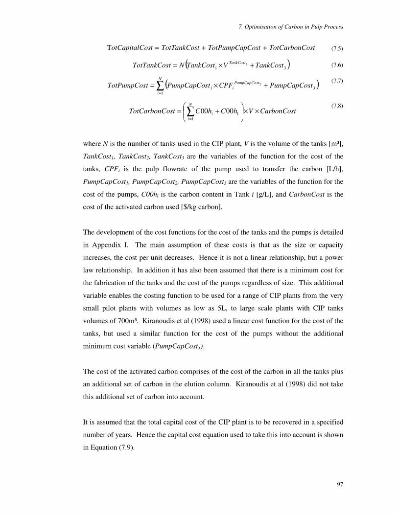
7. Optimisation of Carbon in Pulp Process
97
TotCapitalCost = TotTankCost + TotPumpCapCost + TotCarbonCost (7.5)
( )312 TankCostVTankCostNtTotTankCos TankCost +×= (7.6)
( )∑=
+×=N
i
tPumpCapCosi tPumpCapCosCPFtPumpCapCostTotPumpCos
131
2 (7.7)
CarbonCostVhChCostTotCarbonC
N
ii ××
+= ∑
=1
1
0000 (7.8)
where N is the number of tanks used in the CIP plant, V is the volume of the tanks [m³],
TankCost1, TankCost2, TankCost3 are the variables of the function for the cost of the
tanks, CPFi is the pulp flowrate of the pump used to transfer the carbon [L/h],
PumpCapCost1, PumpCapCost2, PumpCapCost3 are the variables of the function for the
cost of the pumps, C00hi is the carbon content in Tank i [g/L], and CarbonCost is the
cost of the activated carbon used [$/kg carbon].
The development of the cost functions for the cost of the tanks and the pumps is detailed
in Appendix I. The main assumption of these costs is that as the size or capacity
increases, the cost per unit decreases. Hence it is not a linear relationship, but a power
law relationship. In addition it has also been assumed that there is a minimum cost for
the fabrication of the tanks and the cost of the pumps regardless of size. This additional
variable enables the costing function to be used for a range of CIP plants from the very
small pilot plants with volumes as low as 5L, to large scale plants with CIP tanks
volumes of 700m³. Kiranoudis et al (1998) used a linear cost function for the cost of the
tanks, but used a similar function for the cost of the pumps without the additional
minimum cost variable (PumpCapCost3).
The cost of the activated carbon comprises of the cost of the carbon in all the tanks plus
an additional set of carbon in the elution column. Kiranoudis et al (1998) did not take
this additional set of carbon into account.
It is assumed that the total capital cost of the CIP plant is to be recovered in a specified
number of years. Hence the capital cost equation used to take this into account is shown
in Equation (7.9).

7. Optimisation of Carbon in Pulp Process
98
( ) 8000AnnualRateCostTotCapitaltFnCapitalCosdtd ×= (7.9)
where AnnualRate is the percentage of the total capital costs to be recovered per year
and the plant operates for 8000 hours per year. The AnnualRate used in this work is 0.2,
implying that the capital costs is to be fully recovered in 5 years. Kiranoudis et al
(1998) also used a similar function to determine the total annual capital cost of the plant.
The total variable costs (TotVariableCost) of the CIP plant is shown in Equation (7.10).
It consists of the cost of the elution of the carbon (TotElutionCost), the power costs of
the pumps (TotPumpVarCost) and the cost of carbon loss to attrition (CarbonLostCost).
All the costs are in Australian Dollars. Kiranoudis et al (1998) reported the cost of
elution and the power costs of the pumps only.
TotVariableCost = TotElutionCost + TotPumpVarCost + CarbonLossCost (7.10)
The cost of elution is shown in Equation (7.11):
( ) ( )
meTransferTiVhCTCtElutionCos
onCostTotalElutidtd tElutionCos 2
11 001 ××= (7.11)
where ElutionCost1 and ElutionCost2 are the variables of the cost of elution,
TransferTime is the time taken to transfer the carbon out of the tank [h], C1T is the
percentage of the mass of carbon transferred, C00h1 is the carbon content of Tank 1
[g/L], and V is the volume of the tanks [m³]. Again the cost of elution is non-linear and
takes into account the economies of scale of eluting larger masses of carbon. A detailed
description of the development of the cost of elution is in Appendix I. Kiranoudis et al
(1998) used a linear function for the cost of elution.

7. Optimisation of Carbon in Pulp Process
99
The operating cost of the carbon transfer pumps is represented by the power
consumption costs of the pumps and they are expressed in Equations (7.12) and (7.13)
respectively.
36000010.CPFPumpHeadgSGpulpPumpPower ii ××××= (7.12)
( ) PowerCostPumpEff
PumpPowerCostTotPumpVar
dtd
N
ii
×=∑
=1
(7.13)
where PumpPoweri is the power rating of the carbon transfer pump for Tank i [kW],
SGpulp is the specific gravity of the pulp [kg/L], g is the acceleration due gravity [m/s²],
PumpHead is the pump head of the carbon transfer pump [m], CPFi is the flowrate of
the pump used to transfer the carbon [L/h], PumpEff is the efficiency rating of the
pump, and PowerCost is the cost of electrical power [kWh]. Kiranoudis et al (1998)
also reported a similar function with the cost of pumps based on the pumping flowrate.
The final variable cost is for the loss of carbon in the CIP process. This cost was not
reported by Kiranoudis et al (1998). The function for this is shown in Equation (7.14).
( ) 8000ostTotCarbonCCarbonLossCostCarbonLossdtd ×= (7.14)
where the CarbonLoss is a percentage of the mass of carbon lost in the CIP process per
year. The CarbonLoss value of 0.2 was used for this work. The values of all the
costing variables detailed above are summarised in Table 7.1.
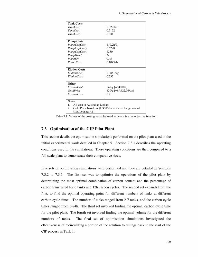
7. Optimisation of Carbon in Pulp Process
100
Tank Costs TankCost1 TankCost2 TankCost3
$3250/m³ 0.5152 $100
Pump Costs PumpCapCost1 PumpCapCost2 PumpCapCost3 PumpHead PumpEff PowerCost
$10.2h/L 0.6298 $250 3m 0.45 0.10kWh
Elution Costs ElutionCost1 ElutionCost2
$3.861/kg 0.737
Other CarbonCost GoldPrice2
CarbonLoss
$4/kg [=$4000/t] $20/g [=$A622.06/oz] 0.2
Notes: 1. All cost in Australian Dollars 2. Gold Price based on $US315/oz at an exchange rate of
US$0.506 to A$1. Table 7.1: Values of the costing variables used to determine the objective function
7.3 Optimisation of the CIP Pilot Plant
This section details the optimisation simulations performed on the pilot plant used in the
initial experimental work detailed in Chapter 5. Section 7.3.1 describes the operating
conditions used in the simulations. These operating conditions are then compared to a
full scale plant to demonstrate their comparative sizes.
Five sets of optimisation simulations were performed and they are detailed in Sections
7.3.2 to 7.3.6. The first set was to optimise the operations of the pilot plant by
determining the most optimal combination of carbon content and the percentage of
carbon transferred for 6 tanks and 12h carbon cycles. The second set expands from the
first, to find the optimal operating point for different numbers of tanks at different
carbon cycle times. The number of tanks ranged from 2-7 tanks, and the carbon cycle
times ranged from 6-24h. The third set involved finding the optimal carbon cycle time
for the pilot plant. The fourth set involved finding the optimal volume for the different
numbers of tanks. The final set of optimisation simulations investigated the
effectiveness of recirculating a portion of the solution to tailings back to the start of the
CIP process in Tank 1.
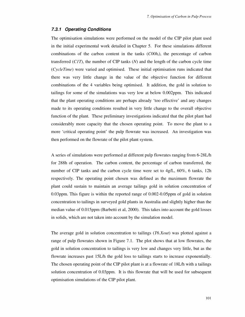
7. Optimisation of Carbon in Pulp Process
101
7.3.1 Operating Conditions
The optimisation simulations were performed on the model of the CIP pilot plant used
in the initial experimental work detailed in Chapter 5. For these simulations different
combinations of the carbon content in the tanks (C00hi), the percentage of carbon
transferred (C1T), the number of CIP tanks (N) and the length of the carbon cycle time
(CycleTime) were varied and optimised. These initial optimisation runs indicated that
there was very little change in the value of the objective function for different
combinations of the 4 variables being optimised. It addition, the gold in solution to
tailings for some of the simulations was very low at below 0.002ppm. This indicated
that the plant operating conditions are perhaps already ‘too effective’ and any changes
made to its operating conditions resulted in very little change to the overall objective
function of the plant. These preliminary investigations indicated that the pilot plant had
considerably more capacity that the chosen operating point. To move the plant to a
more ‘critical operating point’ the pulp flowrate was increased. An investigation was
then performed on the flowrate of the pilot plant system.
A series of simulations were performed at different pulp flowrates ranging from 6-28L/h
for 288h of operation. The carbon content, the percentage of carbon transferred, the
number of CIP tanks and the carbon cycle time were set to 4g/L, 60%, 6 tanks, 12h
respectively. The operating point chosen was defined as the maximum flowrate the
plant could sustain to maintain an average tailings gold in solution concentration of
0.03ppm. This figure is within the reported range of 0.002-0.05ppm of gold in solution
concentration to tailings in surveyed gold plants in Australia and slightly higher than the
median value of 0.015ppm (Barbetti et al, 2000). This takes into account the gold losses
in solids, which are not taken into account by the simulation model.
The average gold in solution concentration to tailings (T6.Xout) was plotted against a
range of pulp flowrates shown in Figure 7.1. The plot shows that at low flowrates, the
gold in solution concentration to tailings is very low and changes very little, but as the
flowrate increases past 15L/h the gold loss to tailings starts to increase exponentially.
The chosen operating point of the CIP pilot plant is at a flowrate of 18L/h with a tailings
solution concentration of 0.03ppm. It is this flowrate that will be used for subsequent
optimisation simulations of the CIP pilot plant.

7. Optimisation of Carbon in Pulp Process
102
0.00
0.05
0.10
0.15
0.20
0.25
0.30
0.35
0.40
5 10 15 20 25 30
[email protected] Au [L/h]
Ave
T6.
Xou
t
Operating point
Figure 7.1: Operating point of the CIP pilot plant
Pulp flowrate and the average gold in solution concentration to tailings in Tank 6
A summary of the operating conditions of the optimisation simulations of the pilot plant
is shown in Table 7.2. The pulp flowrate was set at 18L/h and consisted of silica flour
and water at 40% solids and at a gold in solution concentration rate of 4.45pm. The
initial gold loading on all the carbon was set to 1mg/kg and the initial gold in solution
concentration was 0ppm for all the tanks. The system was simulated for 288h and data
was collected for the final carbon cycle. This value of 288h was chosen as it was a
common denominator value for all 4 carbon cycle times to be investigated – 6, 12, 18
and 24h, and it was also sufficiently long enough for the system to reach steady cyclical
conditions. The objective function was calculated for the last carbon cycle and this
value was used to determine the objective function per annum. It is this per annum
value that is used in the analyses of the results of the simulations.
Pilot Plant Simulation Operating Conditions Total simulation time Variables to be optimised
288h N, C00hi, C1T, CycleTime
Feed Pulp feed Pulp flowrate Gold in solution concentration
Silica flour and water at 40% solids 18L/h 4.45ppm
Initial Conditions Gold loading on carbon Gold in solution concentration
1mg/kg for all tanks 0ppm for all tanks
Table 7.2: Summary of operating conditions for the optimisation simulations of the CIP pilot plant
The simulations to be performed in this chapter represents the results for a pilot scale
CIP plant. To compare the performance of this plant to a larger full scale plant, a
calculation was performed to determine the scale-up factor of the pilot plant to a full

7. Optimisation of Carbon in Pulp Process
103
scale plant. It is assumed that the full scale plant has a throughput of 1.2Mtpa (million
tonnes per annum) with a gold grade of 4.5g/t. The pilot plant throughput is 78.5tpa at a
gold grade of 6.48g/t. Given the throughputs and the gold grades of the two plants, the
pilot plant is 10615 times smaller than the 1.2Mtpa plant. It follows that a larger plant,
for example, with a plant capacity of 2.5Mtpa, will have a larger scale-up factor of
22116. Hence it is important to remember in subsequent discussions of this chapter,
that a $1 change in the objective function of the pilot plant equates to a $10615 change
for an equivalent 1.2Mtpa plant with a gold grade of 4.5g/t.
7.3.2 Set 1 – Optimal Combination of Carbon Content and Percentage
Carbon Transferred
The first set of optimisation simulations performed was to optimise the operating
conditions of the pilot plant. The number of tanks was set to 6 tanks and the carbon
cycle time to 12h (as per the experimental run in Chapter 5). The carbon content and
the percentage of carbon transferred ranged from 2-8g/L and 20-100% respectively. For
the purposes of these simulations the carbon content used is the same for all tanks. The
percentage carbon transferred is the proportion of the carbon that is transferred from
each tank during carbon transfer. This value is expressed as a percentage of the total
amount of carbon in the tank. To ensure a constant total carbon mass balance in the CIP
system, the amount of carbon transferred from each tank is the same.
The results are shown in Figure 7.2. Figure 7.2A shows a 3-dimensional plot of the
objective function, the carbon content and the percentage of carbon transferred. It
indicates that the objective function increases to approximately $8000 and then it seems
to plateau near this value. Figure 7.2B focuses more closely at this ‘plateau region’ with
a 3-dimensional plot of objective functions of $8000 and greater. The maximum
objective function of $8292.67, is at a carbon content and percentage carbon transferred
of 7g/L and 40% respectively. Although the difference between the maximum and
minimum objective function in this plateau region is small, at $300 or less, this value is
magnified approximately 10600 times for a 1.2Mtpa gold plant.

7. Optimisation of Carbon in Pulp Process
104
23
45
67
8
2030
4050
60708090100
-8000
-6000
-4000
-2000
0
2000
4000
6000
8000
10000
Obj
ectiv
e Fu
nctio
n [$
]
Carbon Content [g/L]Carbon Transferred [%]
A
23 4 5 6 7 8
40
60
80
100
8000
8050
8100
8150
8200
8250
8300
Obj
ectiv
e Fu
nctio
n [$
]
Carbon Content [g/L]
Carbon Transferred [%]
B
Figure 7.2: Optimisation simulation results for 6 tanks, 12h carbon cycles
The 7g/L optimal carbon content value is at the lower end of the surveyed gold plants,
which had carbon content values range of 5-15g/L (Barbetti et al, 2000). In addition,
most gold plants do operate with excess carbon in the tanks in order to minimise gold
lost to tailings. Hence additional simulations were performed for higher carbon content
of 9-16g/L and the results are shown in Figure 7.3.
24
68
1012
1416
2040
6080
100
-8000
-6000
-4000
-2000
0
2000
4000
6000
8000
10000
Obj
ectiv
e Fu
nct
ion
[$]
Carbon Content [g/L]
Carbon Transferred [%]
A
24
68
1012
141620
4060
80100
8000
8050
8100
8150
8200
8250
8300
Obj
ectiv
e Fu
nctio
n [$
]
Carbon Content [g/L]
Carbon Transferred [%]
B
Figure 7.3: Optimisation simulation results for 6 tanks, 12h carbon cycles
Figure 7.3 shows two 3-dimensional plots of the objective function, carbon content and
percentage carbon transferred. The range of carbon content and percentage carbon
transferred in these results are 2-16g/L and 20-100% respectively. Figure 7.3A shows
the objective function for the full range of carbon content and percentage of carbon
transferred investigated, and Figure 7.3B shows the objective functions of $8000 and
greater. The plot shows the ‘plateau’ region identified in Figure 7.2A extends further
out to the larger carbon content values investigated in Figure 7.3A.

7. Optimisation of Carbon in Pulp Process
105
Figure 7.3B clearly shows the optimal point at 7g/L carbon content. The plot also
shows that if the carbon content is increased, the value of the objective function will
decrease. Hence there is a cost penalty for using higher carbon content in the CIP
system. As most gold plants do operate with excess carbon in order to minimise gold
losses to tailings, this cost penalty is not perceived to be excessive when compared with
the risk of losing gold to tailings. Normally such a scenario does not occur. However,
if the plant is not operating at ‘normal conditions’ , for example if the plant is
experiencing short circuiting of the pulp flow, an excess amount of carbon in the system
will be able to minimise gold losses to tailings. Hence the magnitude and significance
of the cost penalty of excess carbon depends not only on the cost of the carbon, but to
large extent the operational philosophy adopted, i.e. the perceived risk of not
maintaining an excess amount of carbon in the system, and the mineral properties of the
ore being processed.
Figure 7.3A also shows that an insufficient amount of carbon in the tanks will have a
dramatic influence on the objective function. If the carbon content falls to below 3.5g/L
and 40% carbon transferred, the value of the objective function decreases dramatically.
Figure 7.4 shows the results of the simulations with no capital costs in the objective
function. In this case it is assumed that the capital costs of the plant has already been
recouped and therefore the objective function does not include the cost of the capital
equipment. This mode will be referred to as the operational objective function. The
objective function values are higher than those reported in Figure 7.3, however the
profile is the same for both. This indicates that the optimal plant operating conditions
are similar regardless of whether the cost of capital is included in the objective function.
The maximum operational objective function is $9620.67 at a carbon content and
percentage carbon transferred values of 6g/L and 50% respectively.
Another set of simulations was performed to determine the influence of the price of
carbon on the objective function. Simulations were carried out for 6 tanks, 12h carbon
cycles and at 40% carbon transfer for different carbon content and carbon prices. The
carbon content ranged from 3 to 12g/L and the carbon priced ranged from $3/kg to
$12/kg. The price of carbon used in the previous simulations was $4/kg. The results
are shown in Figure 7.5.

7. Optimisation of Carbon in Pulp Process
106
24
68
1012
1416
2040
6080
100
-8000
-6000
-4000
-2000
0
2000
4000
6000
8000
10000
Obj
ectiv
e F
unct
ion
[$]
Carbon Content [g/L]
Carbon Transferred [%]
A
24
68
1012
1416
2040
6080
100
8000
8400
8800
9200
9600
10000
Obj
ectiv
e Fu
nct
ion
[$]
Carbon Content [g/L]
Carbon Transferred
[%]
B
Figure 7.4: Optimisation simulation results for 6 tanks, 12h carbon cycles with no capital costs in the
objective function
Figure 7.5 shows that the profile of both the objective function and the operational
objective function at different carbon contents does not change with changes in the cost
of carbon. That is, for a certain carbon content value, the objective function remains the
same regardless of the price of carbon. Even when the carbon price was tripled, it still
had very little effect on the objective function. This indicates that the objective function
is not sensitive to changes in the price of carbon as it represents a very small cost
relative to the overall costs of the plant. This is shown in the breakdown of all the costs
of a plant operating at a carbon content of 4g/L, 60% carbon transfer and at 12h carbon
cycles for 1 year of operation in Table 7.3. The capital cost accounts for 72% of the
total costs with the main capital costs attributed to the tanks and the pumps. The cost of
the carbon accounts for only 0.07% of the total capital cost.
3 4 5 6 7 8 9 10 11 123
6
9
12
5000
5500
6000
6500
7000
7500
8000
8500
9000
9500
10000
Obj
ectiv
e Fu
nct
ion
[$]
Carbon Content [g/L]
Carbon Cost [$/kg]
With Capital Costs
3 4 5 6 7 8 9 10 11 123
6
9
12
5000
5500
6000
6500
7000
7500
8000
8500
9000
9500
10000
Ob
ject
ive
Fu
nct
ion
[$]
Carbon Content [g/L]
Carbon Cost [$/kg]
With No Capital Costs
Figure 7.5: Effect of the price of carbon on the objective function and operational objective function.
Optimisation simulation results for 6 tanks, 12h carbon cycles, and 40% carbon transfer.

7. Optimisation of Carbon in Pulp Process
107
Objective Function 8192.67 Gold Revenue 10082.00 Total Cost 1888.27 Capital Cost 1357.00 Variable Cost 458.80 Gold Lost 72.46 Capital Costs - Tanks 862.76 - Pumps 493.35 - Carbon 0.90 Variable Costs - Elution 457.60 - Pump Power 0.23 - Carbon Loss 0.90 in Australian dollars per year
Table 7.3: Costs breakdown for a pilot plant operating at 4g/L carbon content, 60% carbon transfer and at 12h carbon cycles
In conclusion, the maximum objective function for the CIP pilot plant is $8292.67 at a
carbon content and percentage carbon transferred values of 7g/L and 40% respectively.
The maximum operational objective function is $9620.67 at a carbon content and
percentage carbon transferred values of 6g/L and 50% respectively.
7.3.3 Set 2 – Optimal Number of Tanks
This set of optimisation simulations was performed to determine the optimal operating
conditions for different numbers of tanks. The plant was simulated at different carbon
content and percentage carbon transferred values at 6, 12, 18 and 24h carbon cycle
times for 2 to 7 tanks to determine the optimal values.
The results are shown in Figure 7.6 and Table 7.4. Figure 7.6 shows the optimal
objective functions and operational objective functions for 2 to 7 tanks for carbon cycles
of 6, 12, 18 and 24h. Table 7.4 lists these values along with its corresponding carbon
content and percentage carbon transferred values.

7. Optimisation of Carbon in Pulp Process
108
7800
8000
8200
8400
8600
8800
9000
0 1 2 3 4 5 6 7 8
No. Tanks
Obj
ectiv
e Fu
nctio
n [$
]
6h cycle 12h cycle 18h cycle 24h cycle
A: With Capital Costs
8600
88009000
9200
9400
96009800
10000
0 1 2 3 4 5 6 7 8
No. Tanks
Obj
ectiv
e Fu
nctio
n [$
]
6h cycle 12h cycle 18h cycle 24h cycle
B: With No Capital Costs
Figure 7.6: Optimal objective function (A) and operational objective function (B) values for different
numbers of CIP tanks at 6, 12, 18, 24h carbon cycles times.
A: With Capital Costs B: With No Capital Costs No. Tanks % Carbon
Transferred Carbon Content
[g/L]
Objective Function
[$]
No. Tanks % Carbon Transferred
Carbon Content
[g/L]
Objective Function
[$] 6h cycle
2 3 4 5 6 7
10 20 20 20 20 30
26 11 9 7 7 4
8409.33 8486.67 8506.67 8389.33 8213.33 8022.67
6h cycle 2 3 4 5 6 7
10 20 20 20 30 30
24 11 9 7 5 4
8812.00 9117.33 9348.00 9440.00 9488.00 9525.33
12h cycle 2 3 4 5 6 7
20 30 30 40 40 50
27 14 11 7 7 5
8597.33 8709.33 8632.67 8480.67 8292.67 8092.00
12h cycle 2 3 4 5 6 7
20 30 30 40 50 50
27 or 28
14 11 7 6 5
9019.33 9354.67 9492.67 9576.00 9620.67 9651.33
18h cycle
2 3 4 5 6 7
30 40 50 60 60 60
28 15 10 7 7 7
8704.89 8792.44 8693.78 8523.11 8325.33 8104.44
18h cycle 2 3 4 5 6 7
30 40 50 60 70 80
28 15 10 7 6 5
9136.89 9451.11 9585.78 9654.67 9688.89 9714.22
24h cycle
2 3 4 5 6 7
40 50 60 70 70 80
28
15 or 16 11 8 8 6
8779.00 8844.67 8732.00 8550.33 8334.67 8111.67
24h cycle 2 3 4 5 6 7
40 50 60 80 90
100
28 16 11 7 6 5
9219.00 9514.33 9638.00 9703.33 9739.33 9766.33
Table 7.4: Optimal carbon content, percentage carbon transferred, objective function and operational objective function values for different numbers of CIP tanks at 6, 12, 18, 24h carbon cycles times.
Figure 7.6A and Table 7.4A shows that with the exception of the 6h carbon cycle, the
optimal number of tanks for the 12, 18, 24h cycle times is 3 tanks. In addition the
carbon content and the percentage carbon transferred is similar for these three cases.

7. Optimisation of Carbon in Pulp Process
109
For 6h carbon cycle time, the optimal number of tanks is 4. This indicates that 3 or 4
tanks would be sufficient to effectively operate a CIP plant with the same mineralogy
and adsorption kinetics as the pilot plant. The carbon content for all cycle times are
within the 5-15g/L range for gold plants surveyed by AMIRA Project P420A (Barbetti
et al, 2000).
If capital costs are not included in the objective function as shown in Figure 7.6B and
Table 7.4B, the optimal number of tanks is 7. For this case the optimal number of tanks
is the maximum number of tanks available, as the plant fully utilises all of them to
maximise the adsorption of gold onto carbon.
In conclusion, the results of the optimisation of the numbers of tanks indicate that the
optimal number of tanks, if the capital costs are included in the total costs, is 3 or 4
tanks for the carbon cycle times investigated. If the capital costs are not included in the
total costs, then the plant will fully utilise all the tanks available to maximise gold
production.
7.3.4 Set 3 – Optimisation of Carbon Cycle Times
This section analyses the effect of different carbon cycle times on the value of the
objective function. This set also utilises some of the data presented in the previous
section. Figure 7.6 shows the optimal objective function and operational objective
function for different numbers of tanks at different cycle times. Both plots show that as
the cycle time increases, the objective function values increases. In addition, this
behaviour is consistent for all numbers of tanks. Due to this consistent behaviour,
additional cycle times of 30, 36, 42, 48h were investigated for 6 tanks only and the
results are shown in Table 7.5.
Table 7.5 shows that as the carbon cycle time is increased, the values of the percentage
of carbon transferred and the carbon content also increases to accommodate for the
longer cycle time. This means that the amount of carbon transferred increases as the
cycle time is increased. This is shown in Figure 7.7 where the objective functions and
the operational objective functions are plotted with their corresponding masses of the

7. Optimisation of Carbon in Pulp Process
110
carbon transferred. The trends displayed in Figure 7.7 show that as the cycle time
increases, the objective function increases along with the mass of carbon transferred.
A: With Capital Costs B: With No Capital Costs Cycle Time
[h] % Carbon
Transferred Carbon Content
[g/L]
Objective Function
[$]
Cycle Time [h]
% Carbon Transferred
Carbon Content
[g/L]
Objective Function
[$] 6 12 18 24 30 36 42 48
20 40 60 70 80 80 80 80
7 7 7 8 8 9
10 11
8213.33 8292.67 8325.33 8334.67 8383.20 8415.78 8438.29 8454.67
6 12 18 24 30 36 42 48
30 50 70 90
100 100 100 100
5 6 6 6 6 7 8 8
9488.00 9620.67 9688.89 9739.33 9797.07 9830.89 9853.90 9876.00
Table 7.5: Optimal carbon content, percentage carbon transferred, objective function (A) and operational objective function (B) values for 6 tanks at 6-48h carbon cycles times.
8000
8100
8200
8300
8400
8500
0 6 12 18 24 30 36 42 48
Carbon Cycle Time [h]
Obj
ectiv
e F
unct
ion
[$]
0
0.1
0.2
0.3
0.4
0.5
Mass o
f Carbon
Transferred [kg]
Objective Function Mcarbon Transferred
A: With Capital Costs
9400
9500
9600
9700
9800
9900
0 6 12 18 24 30 36 42 48
Carbon Cycle Time [h]
Obj
ectiv
e Fu
nctio
n [$
]
0
0.1
0.2
0.3
0.4
0.5
Mass of C
arbon Transferred [kg]
Objective Function Mcarbon Transferred
B: With No Capital Costs
Figure 7.7: Optimal objective functions and mass of carbon transferred for 6 tanks at 6-48h cycle times
Another cycle time analysis was performed to determine the optimal cycle time when
the number of tanks, carbon content and percentage carbon transferred are set to 6 tanks,
4g/L and 60% respectively. These operating conditions were simulated for 6 to 48h
carbon cycle times and the results are shown in Figure 7.8. The plot shows that the
optimal cycle time for both the objective function and operational objective function is
12h. These results show that there exists an optimal cycle time for combinations of
carbon content and the amount of carbon transferred.

7. Optimisation of Carbon in Pulp Process
111
-4000-2000
02000400060008000
1000012000
0 6 12 18 24 30 36 42 48
Carbon Cycle Time [h]
Ob
ject
ive
Fu
nct
ion
[$]
With Capital Costs With No Capital Costs
Figure 7.8: Objective function for 6 tanks, 4g/L carbon content, 60% carbon transfer at 6-48h cycle times
In conclusion, if the cycle time is increased, the optimal carbon content and percentage
of carbon transferred will also increase to accommodate the increase in carbon residence
time – and as a consequence, the value of the objective function will also rise. This
seems advantageous on the surface, but increasing the carbon cycle time also has other
implications not taken into account by the objective function. Firstly by increasing the
cycle time, the length of time between gold generation, and hence revenue, is increased.
This could have cash flow implications, particularly for small operators that operate at
very low margins. Secondly long cycle times can lead to carbon fouling and thus
reduce the adsorption capacity of the carbon.
For a system with a predetermined carbon content and percentage carbon transferred,
there exists an optimal carbon cycle time as shown in Figure 7.8.
7.3.5 Set 4 – Optimal Volume
The fourth set of optimisation simulations was performed to determine the optimal tank
volume, carbon content and percentage carbon transferred for different number of tanks
running at 12h carbon cycle time. The other cycle times were not investigated as the
previous analysis indicated that an increase in cycle time will result in an increase in the
objective function (as the carbon content and percentage carbon transferred values
change to accommodate for the increase in cycle time), and this trend is consistent for
different numbers of tanks.
Simulations were performed for different percentage carbon transferred and carbon
content for 2 to 7 tanks at tank volumes of 1, 5, 10, 15, 20, 25, 30, 35, and 40L. The

7. Optimisation of Carbon in Pulp Process
112
maximum carbon content used was 30g/L. This value is consistent with the highest
reported target carbon content in surveyed gold plants (O’ Leary and Staunton, 2000).
The optimal operating conditions for different numbers of tanks are listed in Table 7.6.
The table lists the optimal volume, percentage carbon transferred, carbon content and
the objective function for each number of tanks. Table 7.6 shows that the optimal
operating condition is four CIP tanks at 10L volume with a carbon content of 30g/L and
at 40% carbon transfer yielding an objective function of $8900.67 per year. This
objective function is much higher than that reported for the previous investigation of the
optimal number of tanks. The previous study reported an objective function of
$8844.67 for three 40L tanks at 24h carbon cycles (see Section 7.3.3).
No. Tanks Volume [L]
% Carbon Transferred
Carbon Content
[g/L]
Objective Function
[$/yr] 2 3 4 5 6 7
35 20 10 10 5 5
20 30 40 40 70 70
30 27 30 29 30 30
8615.33 8843.33 8900.67 8872.67 8796.67 8782.67
Table 7.6: Optimal volume, percentage carbon transferred, carbon content, objective function values for 2 to 7 tanks at 12h carbon cycles times.
Figure 7.9 shows two 3-dimensional plots of the values of the optimal objective
functions for each number of tanks at volumes of 1L to 40L. Figure 7.9A shows that at
volumes below 5L, the objective function drops dramatically to below zero. As the
volume increases to approximately 5-10L, the objective function seems to plateau to
approximately $8000 for all the numbers of tanks. Figure 7.9B focuses on this plateau
region and shows a plot of objective functions of $8000 and above. This plot indicates
that there are still variations in the plateau region of Figure 7.9A with objective function
values ranging from $8000 to $9000. The maximum objective function area is in the 5
to 15L region and at 3 to 6 tanks. A closer inspection of this maximum area suggests
that there is an optimal total volume for the CIP pilot plant.

7. Optimisation of Carbon in Pulp Process
113
1 5 1015
2025
3035
40 23
45
67
-6000
-4000
-2000
0
2000
4000
6000
8000
10000
Objective Function [$]
Tank Volume [L] No. Tanks
A
15
1015
2025
3035
40 23
45
67
8000
8100
8200
8300
8400
8500
8600
8700
8800
8900
9000
Objective Function [$]
Tank Volume [L]
No. Tanks
B
Figure 7.9: Objective function for different numbers of tanks and volumes at 12h carbon cycle time
Figure 7.10 shows the optimal objective function for each number of tanks and its total
CIP plant volume. It shows that the 3 highest objective functions are at 3, 4 and 5 tanks
and that the corresponding volume range is between 40-60L. Hence there exists an
optimal range for the total CIP plant volume for the pilot plant.
8600
8700
8800
8900
9000
2 3 4 5 6 7
No. Tanks
Obj
ectiv
e Fu
nctio
n [$
/yr]
30
40
50
60
70
Total CIP
Volum
e [L]
Objective Function Total Volume
Figure 7.10: Objective function and total CIP plant volume for each number of tanks
These results suggests that it is not necessarily the number of tanks that is the main
factor in maximising the objective function, but the overall volume of the CIP plant.
That is, once this optimal volume is determined, the number of tanks employed can then
be determined. This overall volume is dependent on the kinetics of the gold adsorption
onto carbon and residence time of the system.

7. Optimisation of Carbon in Pulp Process
114
7.3.6 Set 5 – Plant Recycle
The final set of optimisation simulations was performed to investigate whether
recirculating a portion of the tailings flow would have a positive impact on the objective
function. It was proposed that part of the tailings solution flow be recirculated back into
the first CIP tank. By doing this, the flow of solution through the CIP process increases
and the gold in solution concentration entering Tank 1 would decrease, as it has been
diluted by the recirculating flow. A diagram of this proposal, shown in Figure 7.11,
introduces a new a recirculating variable α, where α is the fraction of the mass flow of
solution recirculated. Equations (7.15) and (7.16), shown below, were added to the
model to accommodate for this recirculating flow, where MFs is the mass flow of
solution through the CIP process [kg/h], RecircSoln is the mass flow of the recirculated
pulp solution [kg/h], and PulpSoln is the original mass flow rate of solution through the
CIP process [kg/h].
To tailings1 2 3 4 5 6
New carbonLoaded carbonto elution
MFslncircSoRe α=
MFslnPulpSo
Figure 7.11: Diagram of recirculating pulp proposal
MFslncircSoRe α= (7.15)
α−
=+=1
lnPulpSolncircSoRelnPulpSoMFs (7.16)
Simulations were performed on a CIP plant consisting of 6 tanks at 12h carbon cycles
for a recirculating fraction of 0.2, 0.4 and 0.6. The results, shown in Table 7.7, list the
optimal operating points for each recirculating fraction investigated. The results show
that recycling part of the pulp flow to tailings back into the CIP process reduces the
value of both the objective function and the operational objective function. This is also
shown in Figure 7.12 where the objective function, gold revenue and total costs for each
recirculating fraction investigated are plotted.

7. Optimisation of Carbon in Pulp Process
115
A: With Capital Costs B: With No Capital Costs
Recirculating Fraction
% Carbon Transferred
Carbon Content
[g/L]
Objective Function
[$]
Recirculating Fraction
% Carbon Transferred
Carbon Content
[g/L]
Objective Function
[$] 0
0.2 0.4 0.6
40 40 40 40
7 8 9
10
8292.67 8247.33 8182.67 8076.00
0 0.2 0.4 0.6
50 50 50 40
6 6 7 8
9620.67 9581.33 9512.00 9398.00
Table 7.7: Results of Plant Recycle. Optimal percentage carbon transferred, carbon content Objective function (A) and operational objective function (B) values for 6 tanks at 12h carbon cycles
times for 0 to 0.6 recirculating fraction.
Figure 7.12 shows that the objective function and operational objective function
decreases as the portion of the pulp recycled increases. This reduction in the objective
function and operational objective function is due to two reasons: an increase in the gold
in solution concentration to tailings, and an increase in the cost of elution. Recycling
tailings pulp increases the gold lost to tailings due to the increased pulp flow through
the plant. The increase in elution costs is due to an increase in the carbon content in
each tank (see Table 7.7) as the amount of pulp recycled increases. In conclusion this
proposal of recycling a portion of the pulp flow does not improve plant performance.
8000
8500
9000
9500
10000
10500
0 0.2 0.4 0.6
Fraction of Pulp Recirculated
Obj
ecti
ve F
unc
tion
and
G
old
Rev
enue
[$/y
r]
1800
1850
1900
1950
2000
2050
Tot
al C
ost [
$/yr
]
Obj(cap. costs) GoldRevenue TotCost
A: With Capital Costs
8000
8500
9000
9500
10000
10500
0 0.2 0.4 0.6
Fraction of Pulp Recirculated
Obj
ecti
ve F
unc
tion
and
G
old
Rev
enue
[$/y
r]
1850
1900
1950
2000
2050
2100
Tot
al C
ost [
$/yr
]Obj(no cap. costs) GoldRevenue TotCost
B: With No Capital Costs
Figure 7.12: Plant recycle simulations: Objective Function (A), Operational Objective Function (B)
Gold Revenue and Total Costs of the optimal point for 0 to 0.6 pulp recycle fraction
7.3.7 Summary of Optimisation of the Pilot Plant
In summary, five sets of optimisation simulations were performed with each set
progressively refining the optimal operating point for the pilot plant. The maximum
objective function of $8900.67 was for 4 tanks of 10L volume, operating at 12h carbon
cycles with a carbon content of 30g/L and at 40% carbon transfer. The proposal of
recirculating the tailings solution back into the CIP system was investigated and it was
found that it did not improve the value of the objective function.

7. Optimisation of Carbon in Pulp Process
116
7.4 Investigation of Carbon Management Strategies
The next two sections will investigate 17 different carbon management strategies.
Firstly, each carbon management strategy will be discussed along with its model
equations. The operating conditions of the simulations will then be outlined, and finally
the results and conclusions of the simulations will be discussed. The simulations are
divided into five sets. Each one will be discussed in further detail in Section 7.5.
7.4.1 Carbon Management Strategies and Model Equations
Four main types of carbon management strategies are investigated: Carousel,
Sequential-Pull, Sequential-Push and Continuous. Stange et al (1990c) also
investigated these 4 strategies, and Kiranoudis et al (1998) investigated 3 - Carousel,
Sequential-Pull and Continuous. For the purpose of this work, these strategies are again
investigated to act as a comparison to additional strategies to be discussed. All of the
different strategies use the same model equations for the rate of adsorption of gold onto
carbon and equilibrium isotherm as described in Section 3.3. A description of the
carbon management strategies, along with associated mass balance equations for the
gold on carbon, gold in solution and mass of carbon for each of the methods is
presented in Section 7.4.1.1 and 7.4.1.2.
7.4.1.1 Carousel Carbon Transfer Method
The carousel carbon movement method involves movement of the carbon only from
tank to tank. In practice, the carbon is ‘transferred’ not by the movement of the carbon,
but by rotating the pulp feed to each tank in the circuit (Stange et al, 1990c). There is
no mixing of the pulp nor carbon, and no partial carbon transfer. That is the percentage
of carbon transferred would be 100%, as the carbon is not moved from the tank until it
is taken out for elution. In addition, only one pump is required to transfer the carbon to
elution.
For the purposes of this investigation, partial carbon transfer will be used to enable
comparisons with the other strategies. In addition, unlike a large scale plant where
partial carbon transfer would be very difficult to achieve for the carousel carbon transfer
method, it can be performed on the CIP pilot plant.

7. Optimisation of Carbon in Pulp Process
117
This method is not commonly used in gold plants for the following reasons:
• There is a risk of the pulp short-circuiting, as the feed tank becomes the tailings tank
during rotation of the pulp feed at carbon transfer. This increases the risk of gold
losses to tailings.
• During carbon transfer, the number of tanks in the system is reduced by one as the
tank with the fully loaded carbon is taken offline to remove the carbon to elution.
When there is one less tank, the gold in solution to tailings will increase.
• From an operational viewpoint, running a carousel plant is more difficult as the inlet
tank changes frequently.
Hence the carousel carbon transfer method is more difficult to implement and it is a
method that leaves little room for error. Even though this is the most efficient method,
it is better to have short-circuiting of carbon inherent in other methods than to lose gold
to tailings.
The mass balance equations for the gold on carbon, gold in solution and mass of carbon
for the carousel carbon transfer method are shown in Equation (7.17) to (7.19). These
equations are the same as those presented in Section 3.3 for the modelling of the initial
pilot plant run.
( )VCRYFCoutYinFCinV
dtCYd
iiiiiiii +−=
(7.17)
ii
i FCoutFCinVdt
dC−=
(7.18)
VCRXoutMFsXinMFsMso
dtdXout
iiiii −−= ln
(7.19)
where i is the ith tank, Yi is the gold loading on the carbon in Tank i [mg/kg], Yini is the
gold loading on the carbon entering tank i [mg/kg], R is the rate of gold adsorption onto
carbon [mg/kg/h], Fcini and Fcouti are the flow of carbon in and out of tank i
respectively during carbon transfer [kg/h], V is the volume of the tanks [m³], Ci is the
carbon content in Tank i [g/L], Xini and Xouti are the gold in solution concentration
entering and leaving Tank i respectively [ppm], and MFs is the mass flowrate of
solution [kg/h].

7. Optimisation of Carbon in Pulp Process
118
A diagram of the flow of carbon and solution between the tanks for the carousel method
is shown in Figure 7.13. The diagram shows two streams flowing in and out of the
tanks, the flow of the pulp solution down the tank train ( ), and the flow of carbon
pumped up the tank train ( ). The diagram also shows no mixing of the pulp flow
from tank to tank, as it does not occur for this carbon transfer method.
Tank (i) Tank (i+1)Tank (i-1) iMFs Xin iMFs Xout
ii YFCout ii YinFCin
Figure 7.13: Flow streams of carbon and solution for the carousel method
7.4.1.2 Sequential and Continuous Carbon Transfer Methods
The most common carbon movement strategy in Australian gold plants is the sequential
carbon transfer method. For this strategy, the carbon is moved at intermittent intervals
in a defined sequence. The carbon is moved from one tank to the next by either
pumping slurry via a centrifugal pump or using an airlift. This means that there is a
backflow of pulp during carbon transfer, flowing counter-current to the pulp flow
through the CIP plant. This is an additional mixing of the pulp not present in the
carousel method.
The two main types of sequential carbon movement are pull and push. For pull the
method, carbon is firstly moved from Tank 1 to elution, then carbon is ‘pulled’ from
Tank 2 to 1, Tank 3 to 2, Tank 4 to 3, Tank 5 to 4, Tank 6 to 5 and finally new carbon is
then put into Tank 6. The ‘push’ method is the reverse of the pull method. Fresh
carbon is firstly put into Tank 6, then carbon is ‘pushed’ up the tank train and the carbon
is then finally removed from Tank 1 to elution.
Continuous carbon movement is where the carbon is pumped continuously from one
tank to the next. This also means that the new carbon is continually being put into Tank
6 and loaded carbon is being continually removed from Tank 1. The strategy is not

7. Optimisation of Carbon in Pulp Process
119
used in gold plants as it requires the slurry to be continuously pumped from tank to
tank. Continuous pumping to transfer carbon breaks down the carbon particles resulting
in high carbon attrition rates. It has been reported in literature as it acts as a basis for
comparison of the other methods, as it will operate at true steady state (Stange et al,
1990c).
The equations for the gold loading on carbon and the carbon content for the continuous
and sequential methods are the same as for the carousel method as shown in Equation
(7.17) and (7.18). The equations for the gold in solution mass balance are shown in
Equations (7.20) to (7.22).
For Tank 1:
( ) ( ) VCRXoutXoutCSFXoutXinMFslnMsodt
dXout1112211
1 −−+−= (7.20)
For Tank (N):
( ) ( ) VCRXoutXinCSFXoutXinMFslnMsodt
dXoutNNNNNNN
N −−+−= (7.21)
For Tank i where i=2 to (N-1):
( ) ( )( ) VCRXoutXoutCSF
XoutXinCSFXoutXinMFslnMsodt
dXout
iiii)i(
iiiiii
−−+
−+−=
++ 11
(7.22)
where CSFi is the flow of solution due to carbon being pumped from Tank i [kg/h].
Although the equations of these two methods are the same, the manner in which the
carbon is moved is different. For sequential carbon transfer, the flows of carbon are
turned on and off as dictated by the sequence of carbon transfer being used. For
continuous carbon transfer, the flows of carbon and it associated flow of solution are
constant and the same for all tanks.
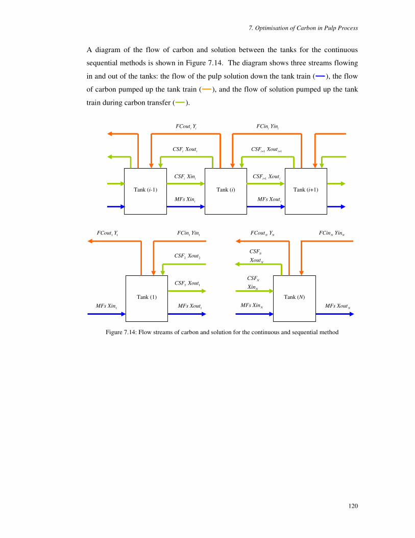
7. Optimisation of Carbon in Pulp Process
120
A diagram of the flow of carbon and solution between the tanks for the continuous
sequential methods is shown in Figure 7.14. The diagram shows three streams flowing
in and out of the tanks: the flow of the pulp solution down the tank train ( ), the flow
of carbon pumped up the tank train ( ), and the flow of solution pumped up the tank
train during carbon transfer ( ).
iMFs Xin iMFs Xout
Tank (i) Tank (i+1)Tank (i-1)
ii XinCSF
ii XoutCSF
ii XoutCSF 1+
11 ++ ii XoutCSF
ii YFCout ii YinFCin
1MFs Xin 1MFs Xout
Tank (1)
12 XoutCSF
22 XoutCSF
11 YFCout 11 YinFCin
NMFs XinNMFs Xout
Tank (N)
N
N
Xin
CSF
N
N
Xout
CSF
NN YFCout NN YinFCin
Figure 7.14: Flow streams of carbon and solution for the continuous and sequential method

7. Optimisation of Carbon in Pulp Process
121
7.4.2 Operating Conditions
The simulation operating conditions for this investigation are the same as those used to
determine the operating point of the CIP pilot plant described in Section 7.3.1 and are
summarised in Table 7.8. The CIP plant consists of six 40L tanks. The plant was
simulated at 12h carbon cycles, for 24 cycles, for a total of 288h. The pulp consists of
40% silica flour, at a flowrate of 18L/h with a gold in solution concentration of
4.45ppm.
The carbon content in each of the CIP tanks is 4g/L which equates to 0.16kg of carbon
in each tank. During carbon transfer 60% (0.096kg) of the total amount of carbon in
each tank is transferred. The initial carbon loading is set to 1mg/kg and all new carbon
put into the plant is of this loading value. The initial gold in solution concentration for
all the tanks is 0ppm.
Pilot Plant Simulation Operating Conditions No. Tanks Total simulation time Time period for each carbon cycle
6 288h 12h
Feed Pulp feed Pulp flowrate Gold in solution concentration
Silica flour and water at 40% solids 18L/h 4.45ppm
Carbon Carbon content in each tank % carbon transferred Mass of carbon in each tank Mass of carbon transferred
4g/L 60% 0.16kg 0.096kg
Initial Conditions Gold loading on carbon Gold in solution concentration
1mg/kg for all tanks 0ppm for all tanks
Table 7.8: Summary of pilot plant operating conditions for the simulation of different carbon management strategies

7. Optimisation of Carbon in Pulp Process
122
7.5 Simulation of Carbon Management Strategies
Five sets of carbon management strategies are investigated. The first set is the
investigation of the four methods outlined in Section 7.4.1 – the Carousel, Sequential-
Pull, Sequential-Push and Continuous methods. The second set investigates different
combinations of sequential carbon movement. The third and fourth sets investigate a
modified version of the sequential carbon movement method where more that one pump
is turned on at a time. That is, the carbon is transferred simultaneously from multiple
tanks in ‘parallel’ . Most of these methods have either been implemented or discussed in
the gold industry. However issues of proprietary knowledge have prevented them being
discussed in the open literature. The final set investigates the proposal of adding new
carbon into the CIP process in other tanks as well as the final tank (Tank 6).
For each carbon movement strategy investigated, a summary sheet of the results is
produced. These are numbered from Simulations 7.1 to 7.17. The simulation
summaries details the operating parameters, a description of the carbon movement
strategy used, and the results of the objective function values. As per previous
optimisation work in Section 7.3, the objective function value for the final cycle was
firstly calculated and then this figure was used to determine the objective function per
year. It is this per annum value that is reported for all simulations performed. A plot of
the changes in mass of carbon in each tank during carbon transfer is also shown.
It must be stressed that although the simulations are not based on a full scale gold plant,
but a small pilot plant scale, it is the comparative differences between the strategies that
are being investigated. It must also be reiterated that this small scale pilot plant is
10600 smaller than a 1.2Mtpa plant. Hence a $1 difference in objective function values
in these investigations is magnified 10600 times in a 1.2Mtpa plant.
The costings are compared with published data in Section 7.5.6 and the conclusions of
the investigation of the five sets of carbon management strategies are presented in
Section 7.5.6.

7. Optimisation of Carbon in Pulp Process
123
7.5.1 Set 1 – Investigation of Carousel, Continuous, Sequential-Pull and
Sequential-Push Carbon Transfer Methods
This first set investigates the Carousel, Continuous, Sequential-Pull, and Sequential-
Push carbon transfer methods. The plots of the gold loading on carbon, gold in solution
concentration and the carbon mass profile for each tank during the final 12h cycle are
shown for the Carousel, Sequential-Pull and Sequential-Push methods in Figure 7.17,
Figure 7.19, and Figure 7.20 respectively. Figure 7.18 shows the plots of the gold
loading on carbon and the gold in solution concentration for the Continuous carbon
transfer method. The simulation results are shown in Simulations 7.1 to 7.4.
Figure 7.15 shows the per annum values of the objective function, gold revenue and
total cost of the four carbon transfer strategies being investigated. The results show that
the Carousel method is the most efficient carbon transfer method, followed by
Continuous, Sequential-Pull and then Sequential-Push, based on the value of the
objective functions and the total costs. These results are consistent with the findings of
Kiranoudis et al (1998). Stange et al (1990b) and Stange (1991) also found that the
Carousel is the most efficient carbon transfer method. Further analysis of the results of
Figure 7.15 and Simulations 7.1 to 7.4 show that gold revenue ranges from $9974 to
$10,082 for the Carousel, Continuous and Sequential-Pull methods, and is only $9879
for the Sequential-Push method. This shows the superiority of the other methods over
Sequential-Push.
7800
8000
8200
8400
8600
8800
Carousel Continous Sequential-pull
Sequential-push
Carbon Transfer Method
Ob
ject
ive
Fu
nct
ion
[$/
yr]
1000
1250
1500
1750
2000
2250
Total C
ost [$/yr]
Objective Function Total Cost
9850
9900
9950
10000
10050
10100
Carousel Continous Sequential-pull
Sequential-push
Carbon Transfer Method
Go
ld R
even
ue
[$/y
r]
Gold Revenue
Figure 7.15: Objective function, gold revenue and total cost per annum for the Carousel, Continuous,
Sequential-Pull and Sequential-Push carbon transfer methods

7. Optimisation of Carbon in Pulp Process
124
The total cost is low for the Carousel method because only one pump is required to
transfer the carbon. The Continuous method’ s costs are lower than the two sequential
methods, again due to lower pump capital costs. For all methods, the same volume of
pulp is pumped to transfer the carbon, however for the Continuous method, the pump
operates at a much lower flowrate. For 60% carbon transfer, 24L of pulp (and carbon)
has to be transferred from one tank to the next for every 12h carbon cycle. Hence for
the Continuous method, the pump operates at a flowrate of 2L/h (pump 24L in 12h), but
for the sequential methods the pulp is pumped in 0.3h and therefore operates at a
flowrate of 80L/h. The large difference in the flowrates of the carbon transfer pumps
accounts for the difference in the total cost value between the Continuous and
Sequential transfer methods.
The variable costs for all the methods were the same. This is to be expected as the
operating conditions were identical for all the methods investigated. That is, the costs
of elution and carbon lost is the same, as the same amount of carbon is being eluted and
used in the CIP process. The cost of the power used is so low compared to the other
costs that any variations between the different methods are negligible.
The Sequential-Pull method is more effective than the Sequential-Push. This is due to
two reasons, a higher gold loading on carbon removed from Tank 1 to elution, and
lower gold losses to tailings. The higher gold loading on carbon removed from Tank 1
is illustrated in Figure 7.16. The plot shows the Tank 1 gold loading on carbon profiles
for the Sequential-Pull and Sequential-Push methods. Although the Sequential-Push
actually has a higher gold loading on carbon averaged over the entire cycle time (see
Figure 7.16A), it is actually lower during the carbon transfer period (see Figure 7.16B).
It is during this carbon transfer period that the gold loading on carbon needs to be at its
maximum point, as it is this batch of carbon that is being eluted for gold. This batch of
carbon sent to elution is at its maximum gold loading range for the Sequential-Pull
method but not for the Push method as illustrated in Figure 7.16B.
For the Sequential-Pull method, the carbon is moved out of Tank 1 before carbon is
moved into the tank from Tank 2. However it is the reverse for Sequential-Push where
carbon is added to Tank 1 (from Tank 2) first, and is then transferred out of Tank 1 to
elution. This increases the amount of carbon in Tank 1 and as a consequence, the

7. Optimisation of Carbon in Pulp Process
125
average gold loading on the carbon is reduced. Hence the batch of carbon sent to
elution for Sequential-Push will have a lower average gold loading on carbon, resulting
in a lower gold revenue value.
5000
6000
7000
8000
9000
10000
0 2 4 6 8 10 12
Time [h]
T1.
Y [
mg
/kg
]
Sequential-pull Sequential-push
5000
6000
7000
8000
9000
10000
10 10.5 11 11.5 12
Time [h]
T1.
Y [
mg
/kg
]
Sequential-pull Sequential-push
s equential-pus htrans fer period
s equential-pull trans fer period
A: For the final carbon cycle B: During Carbon Transfer
Figure 7.16: Gold loading on carbon for the last cycle and during carbon transfer for the Sequential-Pull
and Sequential-Push carbon transfer methods
The Push method also results in an increase in the gold losses to tailings as the carbon
entering Tank 6 no longer acts as ‘scavengers’ for the gold in solution at the end of the
CIP process. By mixing the new carbon with the existing carbon in Tank 6, its
scavenging role has been nullified. However for the Sequential-Pull, the new carbon
enters the system in Tank 6 after the carbon has already been transferred from Tank 6 to
5. Hence the new carbon has less competition for the gold in solution with the existing
carbon in the tank, when compared to the Sequential-Push method. This theory is
supported by the gold lost values of the Sequential-Pull and Sequential-Push at $98 and
$134 respectively.
The next three sets of carbon management strategies investigated will focus on different
variations of the sequential transfer method, as it is this method that is most commonly
used in gold plants.
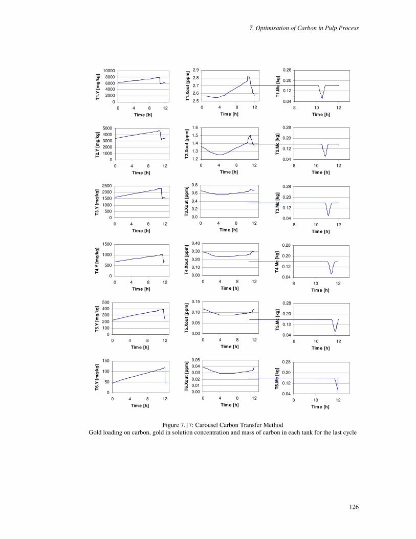
7. Optimisation of Carbon in Pulp Process
126
02000400060008000
10000
0 4 8 12
Time [h]
T1.
Y [
mg
/kg
]
010002000300040005000
0 4 8 12
Time [h]
T2.
Y [m
g/kg
]
0500
1000150020002500
0 4 8 12
Time [h]
T3.Y
[mg/
kg]
0
500
1000
1500
0 4 8 12
Time [h]
T4.
Y [m
g/kg
]2.5
2.6
2.7
2.8
2.9
0 4 8 12
Time [h]
T1.
Xo
ut [
ppm
]
1.2
1.3
1.4
1.5
1.6
0 4 8 12
Time [h]
T2.
Xo
ut [
ppm
]
0.0
0.2
0.4
0.6
0.8
0 4 8 12
Time [h]
T3.
Xo
ut [p
pm
]
0.00
0.10
0.20
0.30
0.40
0 4 8 12
Time [h]
T4.
Xo
ut [
ppm
]
0.04
0.12
0.20
0.28
8 10 12
Time [h]
T1.M
c [k
g]
0.04
0.12
0.20
0.28
8 10 12
Time [h]
T2.
Mc
[kg]
0.04
0.12
0.20
0.28
8 10 12
Time [h]
T3.
Mc
[kg
]0.04
0.12
0.20
0.28
8 10 12
Time [h]
T4.
Mc
[kg
]
0100200300400500
0 4 8 12
Time [h]
T5.
Y [
mg
/kg
]
0
50
100
150
0 4 8 12
Time [h]
T6.
Y [
mg
/kg
]
0.00
0.05
0.10
0.15
0 4 8 12
Time [h]
T5.
Xo
ut
[ppm
]
0.000.010.020.030.040.05
0 4 8 12
Time [h]
T6.
Xou
t [p
pm]
0.04
0.12
0.20
0.28
8 10 12
Time [h]
T5.
Mc
[kg
]
0.04
0.12
0.20
0.28
8 10 12
Time [h]
T6.M
c [k
g]
Figure 7.17: Carousel Carbon Transfer Method
Gold loading on carbon, gold in solution concentration and mass of carbon in each tank for the last cycle

7. Optimisation of Carbon in Pulp Process
127
02000
40006000
800010000
0 100 200 300
Time [h]
T1.
Y [
mg
/kg
]
0
2000
4000
6000
0 100 200 300
Time [h]
T2.
Y [m
g/k
g]
0
1000
2000
3000
0 100 200 300
Time [h]
T3.
Y [m
g/k
g]
0
500
1000
1500
0 100 200 300Time [h]
T4.
Y [
mg/
kg]
0
200
400
600
0 100 200 300Time [h]
T5.
Y [m
g/k
g]
0
50
100
150
200
0 100 200 300Time [h]
T6.
Y [m
g/k
g]
0.0
1.0
2.0
3.0
0 100 200 300
Time [h]
T1.
Xou
t [m
g/k
g]
0.0
0.5
1.0
1.5
2.0
0 100 200 300
Time [h]
T2.X
ou
t [m
g/kg
]
0.00
0.20
0.40
0.60
0.80
0 100 200 300
Time [h]T
3.X
out
[m
g/kg
]
0.00
0.10
0.20
0.30
0.40
0 100 200 300Time [h]
T4.
Xou
t [m
g/k
g]
0.00
0.05
0.10
0.15
0 100 200 300Time [h]
T5.X
ou
t [m
g/k
g]
0.00
0.02
0.04
0.06
0 100 200 300Time [h]
T6.X
ou
t [m
g/k
g]
Figure 7.18: Continuous Carbon Transfer Method
Gold loading on carbon and gold in solution concentration

7. Optimisation of Carbon in Pulp Process
128
02000400060008000
10000
0 4 8 12
Time [h]
T1.
Y [
mg
/kg
]
010002000300040005000
0 4 8 12
Time [h]
T2.
Y [m
g/kg
]
0
1000
2000
3000
0 4 8 12
Time [h]
T3.Y
[mg/
kg]
0
500
1000
1500
0 4 8 12
Time [h]
T4.
Y [m
g/kg
]0.0
1.0
2.0
3.0
0 4 8 12
Time [h]
T1.
Xo
ut [
ppm
]
0.0
0.5
1.0
1.5
2.0
0 4 8 12
Time [h]
T2.
Xo
ut [
ppm
]
0.0
0.5
1.0
1.5
0 4 8 12
Time [h]
T3.
Xo
ut [p
pm
]
0.00
0.20
0.40
0.60
0.80
0 4 8 12
Time [h]
T4.
Xo
ut [
ppm
]
0.04
0.12
0.20
0.28
8 10 12
Time [h]
T1.M
c [k
g]
0.04
0.12
0.20
0.28
8 10 12
Time [h]
T2.
Mc
[kg]
0.04
0.12
0.20
0.28
8 10 12
Time [h]
T3.
Mc
[kg
]0.04
0.12
0.20
0.28
8 10 12
Time [h]
T4.
Mc
[kg
]
0100200300400500
0 4 8 12
Time [h]
T5.
Y [
mg
/kg
]
0
50
100
150
200
0 4 8 12
Time [h]
T6.
Y [
mg
/kg
]
0.00
0.10
0.20
0.30
0 4 8 12
Time [h]
T5.
Xo
ut
[ppm
]
0.00
0.05
0.10
0.15
0 4 8 12
Time [h]
T6.
Xou
t [p
pm]
0.04
0.12
0.20
0.28
8 10 12
Time [h]
T5.
Mc
[kg
]
0.04
0.12
0.20
0.28
8 10 12
Time [h]
T6.M
c [k
g]
Figure 7.19: Sequential-Pull Carbon Transfer Method
Gold loading on carbon, gold in solution concentration and mass of carbon in each tank for the last cycle

7. Optimisation of Carbon in Pulp Process
129
02000400060008000
10000
0 4 8 12
Time [h]
T1.
Y [
mg
/kg
]
0
2000
4000
6000
8000
0 4 8 12
Time [h]
T2.
Y [m
g/kg
]
0
1000
2000
3000
4000
0 4 8 12
Time [h]
T3.Y
[mg/
kg]
0
500
1000
1500
2000
0 4 8 12
Time [h]
T4.
Y [m
g/kg
]0.0
1.0
2.0
3.0
4.0
0 4 8 12
Time [h]
T1.
Xo
ut [
ppm
]
0.0
0.5
1.0
1.5
2.0
0 4 8 12
Time [h]
T2.
Xo
ut [
ppm
]
0.0
0.5
1.0
1.5
0 4 8 12
Time [h]
T3.
Xo
ut [p
pm
]
0.000.100.200.300.400.50
0 4 8 12
Time [h]
T4.
Xo
ut [
ppm
]
0.04
0.12
0.20
0.28
8 10 12
Time [h]
T1.M
c [k
g]
0.04
0.12
0.20
0.28
8 10 12
Time [h]
T2.
Mc
[kg]
0.04
0.12
0.20
0.28
8 10 12
Time [h]
T3.
Mc
[kg
]0.04
0.12
0.20
0.28
8 10 12
Time [h]
T4.
Mc
[kg
]
0200400600800
1000
0 4 8 12
Time [h]
T5.
Y [
mg
/kg
]
0
100
200
300
400
0 4 8 12
Time [h]
T6.
Y [
mg
/kg
]
0.000.050.100.150.200.25
0 4 8 12
Time [h]
T5.
Xo
ut
[ppm
]
0.000.020.040.060.080.10
0 4 8 12
Time [h]
T6.
Xou
t [p
pm]
0.04
0.12
0.20
0.28
8 10 12
Time [h]
T5.
Mc
[kg
]
0.04
0.12
0.20
0.28
8 10 12
Time [h]
T6.M
c [k
g]
Figure 7.20: Sequential-Push Carbon Transfer Method
Gold loading on carbon, gold in solution concentration and mass of carbon in each tank for the last cycle

7. Optimisation of Carbon in Pulp Process
130
Simulation 7.1: Carousel
Simulation Summary
0.04
0.12
0.20
0.28
10 11 12Time [h]
Mc
[kg
]
T1
T2
T3
T4
T5
T6
Mass of carbon in each tank during carbon transfer
Objective Function Results [$/yr] Objective Function 8604.86 Gold Revenue 10082.00 Total Cost 1477.14 - Capital Cost 945.88 - Variable Cost 458.80 - Gold Lost 72.46 T1.Y to elution [mg/kg] 7854 Average T6.Xout [ppm] 0.0321
Note: Only one pump is required to transfer carbon out to elution for a carousel plant.
No. Tanks = 6 Initial Y = 1mg/kg Pulp flow = 18L/h Initial Xout = 0ppm T1.Xin = 4.45ppm C = 4g/L Mc = 0.16kg C1T = 0.6 Mc transferred = 0.096kg Carbon cycle time = 12h Total simulation time = 288h Carbon Transfer Method : Carousel Carbon transferred in the following sequential order: T1 �(OXWLRQ T2 �7� T3 �7� T4 �7� T5 �7� T6 �7� New C in T6
Operating Strategy Description The CIP process was simulated for 288h for 6 tanks. Each tank had a live capacity of 40L, containing 0.16kg of carbon at an initial loading of 1mg/kg. Initial gold in solution concentrations in all the tanks was 0ppm. The pulp feed consisted of 40% silica solids entering the CIP process at 18L/h, at a gold solution concentration of 4.45ppm. Carbon was transferred every 12 hours. 60% of the carbon (0.096kg) in each tank was transferred. The carbon transfer method used was the carousel method with the carbon being ‘pulled’ from the process. Carbon was firstly removed from Tank 1 out to elution, then from Tank 2 to Tank 1, Tanks 3 to Tank 2, Tank 4 to Tank 3, Tank 5 to Tank 4, Tank 6 to Tank 5, and new carbon was put into Tank 6.
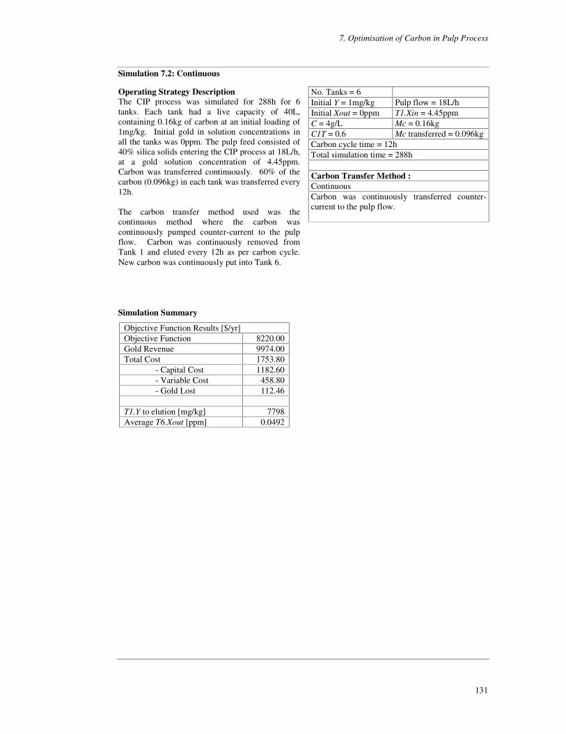
7. Optimisation of Carbon in Pulp Process
131
Simulation 7.2: Continuous
Simulation Summary
Objective Function Results [$/yr] Objective Function 8220.00 Gold Revenue 9974.00 Total Cost 1753.80 - Capital Cost 1182.60 - Variable Cost 458.80 - Gold Lost 112.46 T1.Y to elution [mg/kg] 7798 Average T6.Xout [ppm] 0.0492
No. Tanks = 6 Initial Y = 1mg/kg Pulp flow = 18L/h Initial Xout = 0ppm T1.Xin = 4.45ppm C = 4g/L Mc = 0.16kg C1T = 0.6 Mc transferred = 0.096kg Carbon cycle time = 12h Total simulation time = 288h Carbon Transfer Method : Continuous Carbon was continuously transferred counter-current to the pulp flow.
Operating Strategy Description The CIP process was simulated for 288h for 6 tanks. Each tank had a live capacity of 40L, containing 0.16kg of carbon at an initial loading of 1mg/kg. Initial gold in solution concentrations in all the tanks was 0ppm. The pulp feed consisted of 40% silica solids entering the CIP process at 18L/h, at a gold solution concentration of 4.45ppm. Carbon was transferred continuously. 60% of the carbon (0.096kg) in each tank was transferred every 12h. The carbon transfer method used was the continuous method where the carbon was continuously pumped counter-current to the pulp flow. Carbon was continuously removed from Tank 1 and eluted every 12h as per carbon cycle. New carbon was continuously put into Tank 6.

7. Optimisation of Carbon in Pulp Process
132
Simulation 7.3: Sequential - Pull
Simulation Summary
0.04
0.12
0.20
0.28
10 11 12Time [h]
Mc
[kg
]
T1
T2
T3
T4
T5
T6
Mass of carbon in each tank during carbon transfer
Objective Function Results [$/yr] Objective Function 8142.00 Gold Revenue 10056.67 Total Cost 1914.00 - Capital Cost 1357.00 - Variable Cost 458.80 - Gold Lost 98.22 T1.Y to elution [mg/kg] 7835 Average T6.Xout [ppm] 0.0508
No. Tanks = 6 Initial Y = 1mg/kg Pulp flow = 18L/h Initial Xout = 0ppm T1.Xin = 4.45ppm C = 4g/L Mc = 0.16kg C1T = 0.6 Mc transferred = 0.096kg Carbon cycle time = 12h Total simulation time = 288h Carbon Transfer Method : Sequential - pull Carbon transferred in the following sequential order: T1 �(OXWLRQ T2 �7� T3 �7� T4 �7� T5 �7� T6 �7� New C in T6
Operating Strategy Description The CIP process was simulated for 288h for 6 tanks. Each tank had a live capacity of 40L, containing 0.16kg of carbon at an initial loading of 1mg/kg. Initial gold in solution concentrations in all the tanks was 0ppm. The pulp feed consisted of 40% silica solids entering the CIP process at 18L/h, at a gold solution concentration of 4.45ppm. Carbon was transferred every 12 hours. 60% of the carbon (0.096kg) in each tank was transferred. The carbon transfer method used was the sequential-pull method with the carbon being ‘pulled’ from the process. Carbon was firstly removed from Tank 1 out to elution, then from Tank 2 to Tank 1, Tanks 3 to Tank 2, Tank 4 to Tank 3, Tank 5 to Tank 4, Tank 6 to Tank 5, and new carbon was put into Tank 6.

7. Optimisation of Carbon in Pulp Process
133
Simulation 7.4: Sequential - Push
Simulation Summary
0.04
0.12
0.20
0.28
10 11 12Time [h]
Mc
[kg
]
T1
T2
T3
T4
T5
T6
Mass of carbon in each tank during carbon transfer
Objective Function Results [$/yr] Objective Function 7928.00 Gold Revenue 9878.67 Total Cost 1949.87 - Capital Cost 1357.00 - Variable Cost 458.80 - Gold Lost 134.03 T1.Y to elution [mg/kg] 7698 Average T6.Xout [ppm] 0.0590
No. Tanks = 6 Initial Y = 1mg/kg Pulp flow = 18L/h Initial Xout = 0ppm T1.Xin = 4.45ppm C = 4g/L Mc = 0.16kg C1T = 0.6 Mc transferred = 0.096kg Carbon cycle time = 12h Total simulation time = 288h Carbon Transfer Method : Sequential - push Carbon transferred in the following sequential order: New C in T6 T6 �7� T5 �7� T4 �7� T3 �7� T2 �7� T1 �(OXWLRQ
Operating Strategy Description The CIP process was simulated for 288h for 6 tanks. Each tank had a live capacity of 40L, containing 0.16kg of carbon at an initial loading of 1mg/kg. Initial gold in solution concentrations in all the tanks was 0ppm. The pulp feed consisted of 40% silica solids entering the CIP process at 18L/h, at a gold solution concentration of 4.45ppm. Carbon was transferred every 12 hours. 60% of the carbon (0.096kg) in each tank was transferred. The carbon transfer method used was the sequential-push method with the carbon being ‘pushed’ up the CIP tank train. New carbon was firstly put into Tank 6, then carbon was moved from Tank 6 to Tank 5, Tank 5 to Tank 4, Tank 4 to Tank 3, Tank 3 to Tank 2, Tank 2 to Tank 1, and Tank 1 out to elution.

7. Optimisation of Carbon in Pulp Process
134
7.5.2 Set 2 – Investigation of Different Combinations of Sequential
Carbon Transfer Methods
This set of carbon management strategies investigates three different combinations of
sequential carbon movement. The results are shown in Simulations 7.5 to 7.7 and are
called Sequential 1, 2 and 3 respectively. Figure 7.21 shows the gold revenue, objective
function and the gold lost to tailings of the strategies investigated. The Sequential-Pull
and Sequential-Push values are also included for comparison. The value of the gold lost
is plotted instead of the total cost (as per the previous set) as the variable costs and the
capital costs are the same for all the strategies discussed in this set.
Sequential 1 (Simulation 7.5) and Sequential 2 (Simulation 7.6) are essentially ‘push’
strategies but the carbon is firstly moved out of Tank 1 to elution as it was shown in the
previous section that this results in a higher gold loading on carbon going to elution and
hence higher gold revenue. For Sequential 1, the carbon is firstly moved out of Tank 1
to elution, then the carbon is moved from Tank 6 to 5, new carbon is then put into Tank
6, and then carbon is ‘pushed’ up the tank train from Tank 5 to 4, Tank 4 to 3, Tank 3 to
2, and finally Tank 2 to 1. For Sequential 2, the carbon is firstly moved out of Tank 1 to
elution, new carbon is then added to Tank 6, and then the carbon is ‘pushed’ up the tank
train from Tank 6 to 5, Tank 5 to 4, Tank 4 to 3, Tank 3 to 2,and finally Tank 2 to 1.
The objective function for the Sequential-Push was $7928, but when the push strategy
was modified to form Sequential 1 and 2, the objective functions for these two strategies
are $8031 and $8017 respectively. The results show that adopting a modified push
strategy, whereby the carbon in Tank 1 is removed first, greatly improves the value of
objective function as well as the gold revenue, and also decreases the gold losses to
tailings. However both the Sequential 1 and 2’ s objective functions are still lower than
Sequential-Pull at $8142.
The difference in Sequential 1 and 2 is due to the point that new carbon is added to
Tank 6. For Sequential 1, carbon is added to Tank 6 after carbon is moved from Tank 6
to 5, however it is the reverse for Sequential 2, where the carbon is firstly added to Tank
6 and then it is moved from Tank 6 to 5. This small procedural difference results in a
7. Optimisation of Carbon in Pulp Process
135
higher gold revenue and a lower gold cost for Sequential 1 over Sequential 2 resulting
in a higher objective function for Sequential 1 as shown in Figure 7.21.
The final strategy investigated in this set, Sequential 3 (Simulation 7.7), combines the
above observations of the most optimal point to add new carbon into the process during
carbon transfer with the superior pull method. Sequential 3 adopts essentially a pull
method but carbon is added into the CIP process soon after carbon is removed from
Tank 1 to elution. Hence the carbon strategy for Sequential 3 is as follows. Firstly
carbon is removed from Tank 1 to elution, then carbon is moved from Tank 6 to 5, new
carbon is added to Tank 6, then carbon is ‘pulled’ up the carbon train and carbon is
moved from Tank 2 to 1, then Tank 3 to 2, Tank 4 to 3, and finally Tank 5 to 4. The
strategy results in an improved objective function value $8145 compared with $8142 for
the Sequential-Pull. The value of the gold revenue is slightly lower than the Sequential-
Pull value, but there is a significant improvement in the gold losses to tailings, reducing
from $98 to $93.
The results of this set shows that a combined push-pull carbon management strategy can
result in a higher objective function and lower gold losses. The best carbon
management strategy in the set is Sequential 3.
7900
7950
8000
8050
8100
8150
8200
Sequential-pull
Sequential-push
Sequential1
Sequential2
Sequential3
Carbon Transfer Method
Obj
ecti
ve F
unct
ion
[$/
yr]
80
90
100
110
120
130
140
Go
ld L
ost
[$/y
r]
Objective Function Gold Lost
9850
9900
9950
10000
10050
10100
Sequential-pull
Sequential-push
Sequential1
Sequential2
Sequential3
Carbon Transfer Method
Go
ld R
even
ue
[$/y
r]
Gold Revenue
Figure 7.21: Objective function, gold revenue and gold lost per annum for different combinations of the
sequential carbon transfer method

7. Optimisation of Carbon in Pulp Process
136
Simulation 7.5: Sequential 1
Simulation Summary
0.04
0.12
0.20
0.28
10 11 12Time [h]
Mc
[kg
]
T1
T2
T3
T4
T5
T6
Mass of carbon in each tank during carbon transfer
Objective Function Results [$/yr] Objective Function 8030.67 Gold Revenue 9956.67 Total Cost 1926.27 - Capital Cost 1357.00 - Variable Cost 458.80 - Gold Lost 110.46 T1.Y to elution [mg/kg] 7756 Average T6.Xout [ppm] 0.0487
No. Tanks = 6 Initial Y = 1mg/kg Pulp flow = 18L/h Initial Xout = 0ppm T1.Xin = 4.45ppm C = 4g/L Mc = 0.16kg C1T = 0.6 Mc transferred = 0.096kg Carbon cycle time = 12h Total simulation time = 288h Carbon Transfer Method : Modified sequential - push Carbon transferred in the following sequential order: T1 �(OXWLRQ T6 �7� New C in T6 T5 �7� T4 �7� T3 �7� T2 �7�
Operating Strategy Description The CIP process was simulated for 288h for 6 tanks. Each tank had a live capacity of 40L, containing 0.16kg of carbon at an initial loading of 1mg/kg. Initial gold in solution concentrations in all the tanks was 0ppm. The pulp feed consisted of 40% silica solids entering the CIP process at 18L/h, at a gold solution concentration of 4.45ppm. Carbon was transferred every 12 hours. 60% of the carbon (0.096kg) in each tank was transferred. The carbon transfer method used was a modified sequential-push method. Carbon was firstly removed from Tank 1 out to elution, then carbon was moved from Tank 6 to Tank 5, new carbon added to Tank 6. Carbon was then ‘pushed’ from Tank 5 to Tank 4, Tank 4 to Tank 3, Tank 3 to Tank 2, Tank 2 to Tank 1.

7. Optimisation of Carbon in Pulp Process
137
Simulation 7.6: Sequential 2
Simulation Summary
0.04
0.12
0.20
0.28
10 11 12Time [h]
Mc
[kg
]
T1
T2
T3
T4
T5
T6
Mass of carbon in each tank during carbon transfer
Objective Function Results [$/yr] Objective Function 8017.33 Gold Revenue 9948.00 Total Cost 1931.00 - Capital Cost 1357.00 - Variable Cost 458.80 - Gold Lost 115.20 T1.Y to elution [mg/kg] 7750 Average T6.Xout [ppm] 0.0506
No. Tanks = 6 Initial Y = 1mg/kg Pulp flow = 18L/h Initial Xout = 0ppm T1.Xin = 4.45ppm C = 4g/L Mc = 0.16kg C1T = 0.6 Mc transferred = 0.096kg Carbon cycle time = 12h Total simulation time = 288h Carbon Transfer Method : Modified sequential - push Carbon transferred in the following sequential order: T1 �(OXWLRQ New C in T6 T6 �7� T5 �7� T4 �7� T3 �7� T2 �7�
Operating Strategy Description The CIP process was simulated for 288h for 6 tanks. Each tank had a live capacity of 40L, containing 0.16kg of carbon at an initial loading of 1mg/kg. Initial gold in solution concentrations in all the tanks was 0ppm. The pulp feed consisted of 40% silica solids entering the CIP process at 18L/h, at a gold solution concentration of 4.45ppm. Carbon was transferred every 12 hours. 60% of the carbon (0.096kg) in each tank was transferred. The carbon transfer method used was a modified sequential-push method. Carbon was firstly removed from Tank 1 out to elution, then new carbon added to Tank 6. Carbon was then ‘pushed’ from Tank 6 to Tank 5, Tank 5 to Tank 4, Tank 4 to Tank 3, Tank 3 to Tank 2, Tank 2 to Tank 1.

7. Optimisation of Carbon in Pulp Process
138
Simulation 7.7: Sequential 3
Simulation Summary
0.04
0.12
0.20
0.28
10 11 12Time [h]
Mc
[kg
]
T1
T2
T3
T4
T5
T6
Mass of carbon in each tank during carbon transfer
Objective Function Results [$/yr] Objective Function 8145.33 Gold Revenue 10054.67 Total Cost 1909.33 - Capital Cost 1357.00 - Variable Cost 458.80 - Gold Lost 93.49 T1.Y to elution [mg/kg] 7833 Average T6.Xout [ppm] 0.0385
No. Tanks = 6 Initial Y = 1mg/kg Pulp flow = 18L/h Initial Xout = 0ppm T1.Xin = 4.45ppm C = 4g/L Mc = 0.16kg C1T = 0.6 Mc transferred = 0.096kg Carbon cycle time = 12h Total simulation time = 288h Carbon Transfer Method : Modified sequential - pull Carbon transferred in the following sequential order: T1 �(OXtion T6 �7� New C in T6 T2 �7� T3 �7� T4 �7� T5 �7�
Operating Strategy Description The CIP process was simulated for 288h for 6 tanks. Each tank had a live capacity of 40L, containing 0.16kg of carbon at an initial loading of 1mg/kg. Initial gold in solution concentrations in all the tanks was 0ppm. The pulp feed consisted of 40% silica solids entering the CIP process at 18L/h, at a gold solution concentration of 4.45ppm. Carbon was transferred every 12 hours. 60% of the carbon (0.096kg) in each tank was transferred. The carbon transfer method used was a modified sequential-pull method. Carbon was firstly removed from Tank 1 out to elution, then carbon was moved from Tank 6 to Tank 5, and new carbon was put into Tank 6. Carbon was then ‘pulled’ from Tank 2 to Tank 1, Tank 3 to Tank 2, Tank 4 to Tank 3, Tank 5 to Tank 4.

7. Optimisation of Carbon in Pulp Process
139
7.5.3 Set 3 – Investigation of Parallel Carbon Transfer Methods
Many gold plants do adopt the sequential carbon transfer method. However due to the
length of time required to transfer the carbon sequentially, some plants adopt a modified
version of the sequential carbon transfer method, whereby more than one carbon
transfer pump is turned on at a time. That is, the carbon is transferred simultaneously
from multiple tanks in ‘parallel’ . For example if a ‘pull’ strategy is adopted, carbon is
pumped from Tank 1 to elution, Tank 3 to 2, and Tank 5 to 4 all at the same time. Then
the carbon from the other three tanks are transferred, that is from Tank 2 to 1, Tank 4 to
3 and Tank 6 to 5 and finally new carbon is put into Tank 6. This method reduces the
carbon cycle time by ���
Transferring carbon from every second tank (i.e. Tanks 1, 3, 5 or Tanks 2, 4, 6) ensures
that the carbon does not short-circuit and is moved only one tank up the CIP train.
Figure 7.22 shows this carbon transfer method graphically. The three sequences of
carbon movement are colour coded. The first part of the carbon transfer where carbon
is transferred from Tanks 1, 3, 5 is coded blue ( ); the second part where carbon is
transferred from Tanks 2, 4, 6 is red ( ); and third and final part where new carbon is
added into Tank 6 is green ( ). Hence this third set of carbon transfer methods will
investigate different ‘parallel’ carbon movement strategies.
1 2 3 4 5 6
New carbonLoaded carbonto elution
1 1 12 2 2 3
Figure 7.22: Example of the Parallel carbon transfer method
Four strategies will be investigated and they are labelled Parallel 1, 2, 3, and 4. The
results of the simulations for the four parallel strategies are shown in Simulations 7.8 to
7.11. The simulation summaries also include a diagram of the carbon transfer method
similar to Figure 7.22.
The first two strategies, Parallel 1 and Parallel 2, are of the pull and push strategies
respectively and Parallel 3 and 4 are combinations of both the push and pull strategy.
For Parallel 1, the carbon is firstly transferred from Tanks 1, 3, 5, then from Tanks 2, 4,

7. Optimisation of Carbon in Pulp Process
140
6 and finally new carbon is put into Tank 6. Parallel 2 adopts a push strategy where by
new carbon is firstly put into Tank 6, then carbon is transferred from Tanks 2, 4, 6 and
finally from Tanks 1, 3, 5. Parallel 3 uses a modified pull strategy, but new carbon is
firstly added to Tank 6, then carbon is transferred from Tanks 1, 3, 5, and finally from
Tanks 2, 4, 6. Parallel 4, is another modified pull strategy with the new carbon added in
between the two tank transfer periods, that is, the carbon is firstly transferred from
Tanks 1, 3, 5, then new carbon is put into Tank 6, and finally carbon is moved from
Tanks 2, 4, 6. Figure 7.23 shows the gold revenue, objective function and the gold lost
to tailings of these four carbon management strategies. The Sequential-Pull method
results are also included as a comparison.
8000
8025
8050
8075
8100
8125
8150
Sequential-pull
Parallel 1 Parallel 2 Parallel 3 Parallel 4
Carbon Transfer Method
Ob
ject
ive
Fu
nct
ion
[$/
yr]
95
100
105
110
115
120
125
Go
ld L
ost
[$/
yr]
Objective Function Gold Lost
9950
9975
10000
10025
10050
10075
Sequential-pull
Parallel 1 Parallel 2 Parallel 3 Parallel 4
Carbon Transfer Method
Go
ld R
even
ue
[$/y
r]
Gold Revenue
Figure 7.23: Objective function, gold revenue and gold lost per annum of different combinations of the 3
tank parallel carbon transfer method
The results show that the objective functions for Parallel 3 and 4 are almost the same at
$8081 and $8083 respectively. It is higher for Parallel 1 at $8093 and Parallel 2 has the
lowest objective function value of $8025. The low objective function value of Parallel
2 is to be expected, as it adopted a push strategy. This is confirmed by its high gold
losses to tailings as shown in Figure 7.23. Parallel 3 and 4 adopted a carbon movement
strategy similar to Sequential 3, the best sequential carbon management strategy as
previously discussed in Section 7.5.2. However this does not result in a higher
objective function when compared with the pull strategy for Parallel 1.
The objective functions of all the Parallel strategies are less than for the Sequential-Pull
method. This shows that the Sequential-Pull method is more effective than any of the
Parallel methods and that there is a cost penalty in adopting the Parallel method over the
Sequential-Pull method.

7. Optimisation of Carbon in Pulp Process
141
Simulation 7.8: Parallel 1 - 3 Tanks Parallel Transfer
1 2 3 4 5 6
New carbonLoaded carbonto elution
1 1 12 2 2 3
Carbon transfer sequence - Parallel Pull Simulation Summary
0.04
0.12
0.20
0.28
10 11 12Time [h]
Mc
[kg
] T1,3,5
T2,4
T6
Mass of carbon in each tank during carbon transfer
Objective Function Results [$] Objective Function 8092.67 Gold Revenue 10008.67 Total Cost 1915.73 - Capital Cost 1357.00 - Variable Cost 458.80 - Gold Lost 99.93 T1.Y to elution [mg/kg] 7797 Average T6.Xout [ppm] 0.0482
No. Tanks = 6 Initial Y = 1mg/kg Pulp flow = 18L/h Initial Xout = 0ppm T1.Xin = 4.45ppm C = 4g/L Mc = 0.16kg C1T = 0.6 Mc transferred = 0.096kg Carbon cycle time = 12h Total simulation time = 288h Carbon Transfer Method : Parallel - pull Carbon transferred in the following sequential order: T1 �(OXWLRQ��7�� �7���7�� �7�� T2 �7���7�� �7���7�� �7�� New C in T6 * carbon moved simultaneously from these three tanks
Operating Strategy Description The CIP process was simulated for 288h for 6 tanks. Each tank had a live capacity of 40L, containing 0.16kg of carbon at an initial loading of 1mg/kg. Initial gold in solution concentrations in all the tanks was 0ppm. The pulp feed consisted of 40% silica solids entering the CIP process at 18L/h, at a gold solution concentration of 4.45ppm. Carbon was transferred every 12 hours. 60% of the carbon (0.096kg) in each tank was transferred. The carbon transfer method used was the parallel-pull method. Firstly carbon was simultaneously removed from Tank 1 out to elution, Tank 3 to Tank 2 and from Tank 5 to Tank 4. Then carbon was simultaneously moved from Tank 2 to Tank 1, Tank 4 to Tank 3 and from Tank 6 to Tank 5. Finally new carbon was added to Tank 6.

7. Optimisation of Carbon in Pulp Process
142
Simulation 7.9: Parallel 2 - 3 Tanks Parallel Transfer
Loaded carbonto elution
1 2 3 4 5 6
New carbon3 3 32 2 2 1
Carbon transfer sequence - Parallel Push Simulation Summary
0.04
0.12
0.20
0.28
10 11 12Time [h]
Mc
[kg
] T1,3,5
T2,4
T6
Mass of carbon in each tank during carbon transfer
Objective Function Results [$] Objective Function 8025.33 Gold Revenue 9960.67 Total Cost 1935.87 - Capital Cost 1357.00 - Variable Cost 458.80 - Gold Lost 120.13 T1.Y to elution [mg/kg] 7762 Average T6.Xout [ppm] 0.0524
No. Tanks = 6 Initial Y = 1mg/kg Pulp flow = 18L/h Initial Xout = 0ppm T1.Xin = 4.45ppm C = 4g/L Mc = 0.16kg C1T = 0.6 Mc transferred = 0.096kg Carbon cycle time = 12h Total simulation time = 288h Carbon Transfer Method : Parallel - push Carbon transferred in the following sequential order: New C in T6 T2 �7���7�� �7���7�� �7�� T1 �(OXWLRQ��7�� �7���7�� �7�� * carbon moved simultaneously from these three tanks
Operating Strategy Description The CIP process was simulated for 288h for 6 tanks. Each tank had a live capacity of 40L, containing 0.16kg of carbon at an initial loading of 1mg/kg. Initial gold in solution concentrations in all the tanks was 0ppm. The pulp feed consisted of 40% silica solids entering the CIP process at 18L/h, at a gold solution concentration of 4.45ppm. Carbon was transferred every 12 hours. 60% of the carbon (0.096kg) in each tank was transferred. The carbon transfer method used was the Parallel-push method. Firstly new carbon was added to Tank 6. Then carbon was simultaneously moved from Tank 2 to Tank 1, Tank 4 to Tank 3 and from Tank 6 to Tank 5. Finally carbon was simultaneously removed from Tank 1 out to elution, Tank 3 to Tank 2 and from Tank 5 to Tank 4.

7. Optimisation of Carbon in Pulp Process
143
Simulation 7.10: Parallel 3 - 3 Tanks Parallel Transfer
Loaded carbonto elution
1 2 3 4 5 6
New carbon2 2 23 3 3 1
Carbon transfer sequence - Parallel push/pull combination Simulation Summary
Objective Function Results [$] Objective Function 8081.33 Gold Revenue 10000.67 Total Cost 1918.93 - Capital Cost 1357.00 - Variable Cost 458.80 - Gold Lost 103.09 T1.Y to elution [mg/kg] 7791 Average T6.Xout [ppm] 0.0481
11 11.5 12
Time [h]
T6
T2,4
T1,3,5
Mass of carbon profiles of the CIP
tanks during carbon transfer
No. Tanks = 6 Initial Y = 1mg/kg Pulp flow = 18L/h Initial Xout = 0ppm T1.Xin = 4.45ppm C = 4g/L Mc = 0.16kg C1T = 0.6 Mc transferred = 0.096kg Carbon cycle time = 12h Total simulation time = 288h Carbon Transfer Method : Modified parallel - pull Carbon transferred in the following sequential order: New C in T6 T1 �(OXWLRQ��7�� �7���7�� �7�� T2 �7���7�� �T3, T6 �7�� * carbon moved simultaneously from these three tanks
Operating Strategy Description The CIP process was simulated for 288h for 6 tanks. Each tank had a live capacity of 40L, containing 0.16kg of carbon at an initial loading of 1mg/kg. Initial gold in solution concentrations in all the tanks was 0ppm. The pulp feed consisted of 40% silica solids entering the CIP process at 18L/h, at a gold solution concentration of 4.45ppm. Carbon was transferred every 12 hours. 60% of the carbon (0.096kg) in each tank was transferred. The carbon transfer method used was a modified parallel-pull method. Firstly new carbon was added to Tank 6. Then carbon was simultaneously removed from Tank 1 out to elution, Tank 3 to Tank 2 and from Tank 5 to Tank 4. Finally carbon was simultaneously moved from Tank 2 to Tank 1, Tank 4 to Tank 3 and from Tank 6 to Tank 5.

7. Optimisation of Carbon in Pulp Process
144
Simulation 7.11: Parallel 4 - 3 Tanks Parallel Transfer
Loaded carbonto elution
1 2 3 4 5 6
New carbon1 1 13 3 23
Carbon transfer sequence - Parallel push/pull combination Simulation Summary
Objective Function Results [$] Objective Function 8082.67 Gold Revenue 10002.67 Total Cost 1919.73 - Capital Cost 1357.00 - Variable Cost 458.80 - Gold Lost 103.97 T1.Y to elution [mg/kg] 7793 Average T6.Xout [ppm] 0.0487
No. Tanks = 6 Initial Y = 1mg/kg Pulp flow = 18L/h Initial Xout = 0ppm T1.Xin = 4.45ppm C = 4g/L Mc = 0.16kg C1T = 0.6 Mc transferred = 0.096kg Carbon cycle time = 12h Total simulation time = 288h Carbon Transfer Method : Modified parallel - pull Carbon transferred in the following sequential order: T1 �(OXWLRQ��7�� �7���7�� �7�� New C in T6 T2 �7���7�� �7���7�� �7�� * carbon moved simultaneously from these three tanks
Operating Strategy Description The CIP process was simulated for 288h for 6 tanks. Each tank had a live capacity of 40L, containing 0.16kg of carbon at an initial loading of 1mg/kg. Initial gold in solution concentrations in all the tanks was 0ppm. The pulp feed consisted of 40% silica solids entering the CIP process at 18L/h, at a gold solution concentration of 4.45ppm. Carbon was transferred every 12 hours. 60% of the carbon (0.096kg) in each tank was transferred. The carbon transfer method used was a modified parallel-pull method. Firstly carbon was simultaneously removed from Tank 1 out to elution, Tank 3 to Tank 2 and from Tank 5 to Tank 4. Then new carbon was added to Tank 6. Finally carbon was simultaneously moved from Tank 2 to Tank 1, Tank 4 to Tank 3 and from Tank 6 to Tank 5.
11 11.5 12
Time [h]
T6
T1,3,5
T2,4
Mass of carbon profiles of the CIP
tanks during carbon transfer

7. Optimisation of Carbon in Pulp Process
145
7.5.4 Set 4 – Further Investigation Parallel Carbon Transfer Methods
This section investigates another form of parallel carbon transfer where carbon is
transferred from two tanks at a time instead of three. Three strategies are investigated
and they are labelled Parallel 5, 6 and 7. The results of the simulations of these
strategies are shown in Simulations 7.12 to 7.14. The simulation summaries also
contain a diagram of the carbon movement strategy adopted.
Parallel 5 adopts a pull carbon movement strategy where the carbon is firstly transferred
out of Tanks 1 and 4, then Tanks 2 and 5, then Tanks 3 and 6. Finally new carbon is put
into Tank 6. Parallel 6 adopts a modified pull carbon movement strategy that is similar
to Sequential 3, the sequential carbon management strategy with the highest objective
function. The carbon movement strategy for Parallel 6 is as follows. Carbon is firstly
moved out of Tanks 1 and 6 and new carbon is put into Tank 6. Then carbon is pulled
up the tank train with carbon being moved out of Tanks 2 and 4, and then Tanks 3 and
5. This carbon strategy is similar to Sequential 3 where the first two sequences moves
carbon out of Tank 1 and then out of Tank 6. Then new carbon is added into Tank 6,
and then the carbon is sequentially pulled up the tank train by moving carbon out of
Tank 2, then Tank 3, Tank 4, and finally Tank 5.
Parallel 7 adopts the same pull strategy as Parallel 5, except the tank pairings have been
changed to see whether it has an effect on the objective function. For Parallel 7, the
Tank pairings are Tank 1 and 3, 2 and 5, and 4 and 6. Hence the carbon movement
strategy for Parallel 7 is as follows. Carbon is firstly moved out of Tanks 1 and 3, then
Tanks 2 and 5, then Tanks 4 and 6, and finally new carbon is put into Tank 6.
Figure 7.24 shows the plots of the objective function, gold lost and gold revenue for
these three parallel strategies. The results for Sequential 3 and Parallel 1, the best
sequential and 3-tank parallel strategies respectively, are also included as a comparison.
The objective functions for Parallel 5, 6, and 7 are $8131, $8127 and $8093
respectively. They are all lower than Sequential 3 at $8145, and are equal to or greater
than the objective function for Parallel 1 at $8093. These results again confirm the
superiority of the sequential transfer method over the parallel methods. The results also
show that, overall, the parallel carbon movement with two tanks will result in a higher
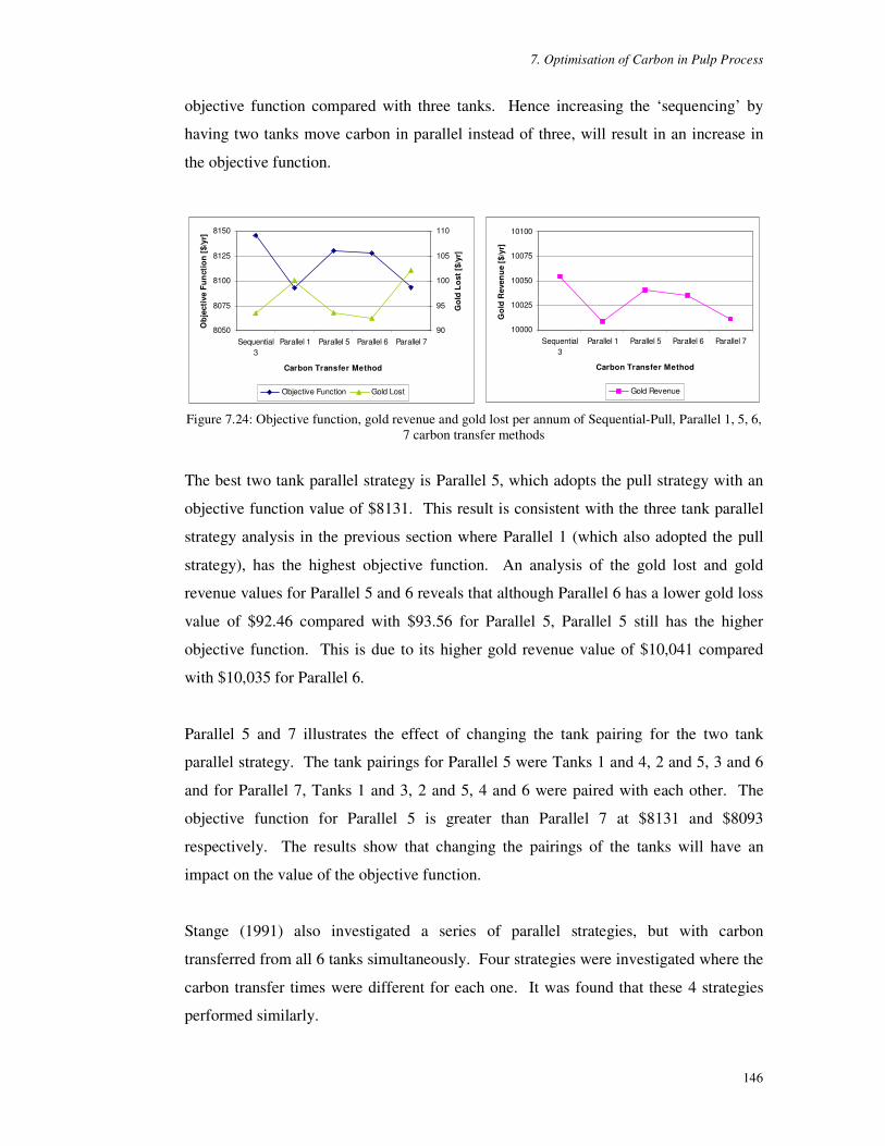
7. Optimisation of Carbon in Pulp Process
146
objective function compared with three tanks. Hence increasing the ‘sequencing’ by
having two tanks move carbon in parallel instead of three, will result in an increase in
the objective function.
10000
10025
10050
10075
10100
Sequential3
Parallel 1 Parallel 5 Parallel 6 Parallel 7
Carbon Transfer Method
Go
ld R
even
ue
[$/y
r]
Gold Revenue
8050
8075
8100
8125
8150
Sequential3
Parallel 1 Parallel 5 Parallel 6 Parallel 7
Carbon Transfer Method
Ob
ject
ive
Fu
nct
ion
[$/
yr]
90
95
100
105
110
Go
ld L
ost
[$/
yr]
Objective Function Gold Lost
Figure 7.24: Objective function, gold revenue and gold lost per annum of Sequential-Pull, Parallel 1, 5, 6,
7 carbon transfer methods
The best two tank parallel strategy is Parallel 5, which adopts the pull strategy with an
objective function value of $8131. This result is consistent with the three tank parallel
strategy analysis in the previous section where Parallel 1 (which also adopted the pull
strategy), has the highest objective function. An analysis of the gold lost and gold
revenue values for Parallel 5 and 6 reveals that although Parallel 6 has a lower gold loss
value of $92.46 compared with $93.56 for Parallel 5, Parallel 5 still has the higher
objective function. This is due to its higher gold revenue value of $10,041 compared
with $10,035 for Parallel 6.
Parallel 5 and 7 illustrates the effect of changing the tank pairing for the two tank
parallel strategy. The tank pairings for Parallel 5 were Tanks 1 and 4, 2 and 5, 3 and 6
and for Parallel 7, Tanks 1 and 3, 2 and 5, 4 and 6 were paired with each other. The
objective function for Parallel 5 is greater than Parallel 7 at $8131 and $8093
respectively. The results show that changing the pairings of the tanks will have an
impact on the value of the objective function.
Stange (1991) also investigated a series of parallel strategies, but with carbon
transferred from all 6 tanks simultaneously. Four strategies were investigated where the
carbon transfer times were different for each one. It was found that these 4 strategies
performed similarly.

7. Optimisation of Carbon in Pulp Process
147
Simulation 7.12: Parallel 5 - 2 Tanks Parallel Transfer
Loaded carbonto elution
1 2 3 4 5 6
New carbon1 43 322 1
Carbon movement sequence and the mass of carbon moved during transfer from each tank Simulation Summary
No. Tanks = 6 Initial Y = 1mg/kg Pulp flow = 18L/h Initial Xout = 0ppm T1.Xin = 4.45ppm C = 4g/L Mc = 0.16kg C1T = 0.6 Mc transferred = 0.096kg Carbon cycle time = 12h Total simulation time = 288h Carbon Transfer Method : Parallel - pull Carbon transferred in the following sequential order: T1 �(OXWLRQ��7�� �7�� T2 �7���7�� �7�� T3 �7���7�� �7�� New C in T6 * carbon moved simultaneously from these two tanks
Objective Function Results [$] Objective Function 8130.67 Gold Revenue 10040.67 Total Cost 1909.40 - Capital Cost 1357.00 - Variable Cost 458.80 - Gold Lost 93.56 T1.Y to elution [mg/kg] 7822 Average T6.Xout [ppm] 0.0468
11 11.5 12
Time [h]
T1,4
T2,5
T3
T6
Mass of carbon profiles of the CIP tanks during carbon transfer
Operating Strategy Description The CIP process was simulated for 288h for 6 tanks. Each tank had a live capacity of 40L, containing 0.16kg of carbon at an initial loading of 1mg/kg. Initial gold in solution concentrations in all the tanks was 0ppm. The pulp feed consisted of 40% silica solids entering the CIP process at 18L/h, at a gold solution concentration of 4.45ppm. Carbon was transferred every 12 hours. 60% of the carbon (0.096kg) in each tank was transferred. The carbon transfer method used was a parallel-pull method. Firstly carbon was simultaneously removed from Tank 1 out to elution, and from Tank 4 to Tank 3. Then carbon was simultaneously moved from Tank 2 to Tank 1, and from Tank 5 to Tank 4. Then carbon was simultaneously moved from Tank 3 to Tank 2, and from Tank 6 to Tank 5. Finally new carbon was added to Tank 6.

7. Optimisation of Carbon in Pulp Process
148
Simulation 7.13: Parallel 6 - 2 Tanks Parallel Transfer
1 2 3 4 5 6
New carbonLoaded carbonto elution
1 4 43 3 1 2
Carbon movement sequence and the mass of carbon moved during transfer from each tank Simulation Summary
No. Tanks = 6 Initial Y = 1mg/kg Pulp flow = 18L/h Initial Xout = 0ppm T1.Xin = 4.45ppm C = 4g/L Mc = 0.16kg C1T = 0.6 Mc transferred = 0.096kg Carbon cycle time = 12h Total simulation time = 288h Carbon Transfer Method : Modified parallel - pull Carbon transferred in the following sequential order: T1 �(OXWLRQ��7�� �7�� New C in T6 T2 �7���7�� �7�� T3 �7���7�� �7�� * carbon moved simultaneously from these two tanks
Objective Function Results [$] Objective Function 8127.33 Gold Revenue 10035.33 Total Cost 1908.27 - Capital Cost 1357.00 - Variable Cost 458.80 - Gold Lost 92.46 T1.Y to elution [mg/kg] 7818 Average T6.Xout [ppm] 0.0399
Operating Strategy Description The CIP process was simulated for 288h for 6 tanks. Each tank had a live capacity of 40L, containing 0.16kg of carbon at an initial loading of 1mg/kg. Initial gold in solution concentrations in all the tanks was 0ppm. The pulp feed consisted of 40% silica solids entering the CIP process at 18L/h, at a gold solution concentration of 4.45ppm. Carbon was transferred every 12 hours. 60% of the carbon (0.096kg) in each tank was transferred. The carbon transfer method used was a modified parallel-pull method. Firstly carbon was simultaneously removed from Tank 1 out to elution, and from Tank 6 to Tank 5. Then new carbon was added to Tank 6. Then carbon was simultaneously moved from Tank 2 to Tank 1, and from Tank 4 to Tank 3. Finally carbon was simultaneously moved from Tank 3 to Tank 2, and from Tank 5 to Tank 4.
11 11.5 12
Time [h]
T1
T2,4
T3
T5
T6
Mass of carbon profiles of the CIP tanks during carbon transfer

7. Optimisation of Carbon in Pulp Process
149
Simulation 7.14: Parallel 7 - 2 Tanks Parallel Transfer
1 2 3 4 5 6
New carbonLoaded carbonto elution
1 43 322 1
Carbon movement sequence and the mass of carbon moved during transfer from each tank Simulation Summary
No. Tanks = 6 Initial Y = 1mg/kg Pulp flow = 18L/h Initial Xout = 0ppm T1.Xin = 4.45ppm C = 4g/L Mc = 0.16kg C1T = 0.6 Mc transferred = 0.096kg Carbon cycle time = 12h Total simulation time = 288h Carbon Transfer Method : Parallel - pull Carbon transferred in the following sequential order: T1 �(OXWLRQ��7�� �7�� T2 �7���7�� �7�� T4 �7���7�� �7�� New C in T6 * carbon moved simultaneously from these two tanks
Objective Function Results [$] Objective Function 8093.33 Gold Revenue 10011.33 Total Cost 1918.07 - Capital Cost 1357.00 - Variable Cost 458.80 - Gold Lost 102.24 T1.Y to elution [mg/kg] 7800 Average T6.Xout [ppm] 0.0494
11 11.5 12
Time [h]
T1
T2
T3
T4
T5
T6
Mass of carbon profiles of the CIP tanks during carbon transfer
Operating Strategy Description The CIP process was simulated for 288h for 6 tanks. Each tank had a live capacity of 40L, containing 0.16kg of carbon at an initial loading of 1mg/kg. Initial gold in solution concentrations in all the tanks was 0ppm. The pulp feed consisted of 40% silica solids entering the CIP process at 18L/h, at a gold solution concentration of 4.45ppm. Carbon was transferred every 12 hours. 60% of the carbon (0.096kg) in each tank was transferred. The carbon transfer method used was a parallel-pull method. Firstly carbon was simultaneously removed from Tank 1 out to elution, and from Tank 3 to Tank 2. Then carbon was simultaneously moved from Tank 2 to Tank 1, and from Tank 5 to Tank 4. Then carbon was simultaneously moved from Tank 4 to Tank 3, and from Tank 6 to Tank 5. Finally new carbon was added to Tank 6.

7. Optimisation of Carbon in Pulp Process
150
7.5.5 Set 5 – Investigation of adding fresh carbon to Tanks 1, 3 and 5
The final set of carbon management strategies to be investigated is the proposal of
adding new carbon to other tanks. For this proposal half of the fresh carbon is added
into the CIP system at Tank 6, and the other half is added to either Tanks 1, 3 or 5. This
is simulated using the sequential carbon transfer strategy that yielded the highest
objective function, which is the carbon strategy used in Sequential 3.
The results of the simulations of these strategies are summarised in Simulations 7.15 to
7.17, and are called Sequential 4, 5 and 6. For Sequential 4, new carbon is added into
Tanks 1 and 6, for Sequential 5, new carbon is added into Tanks 3 and 6, and for
Sequential 6, new carbon is added into Tanks 5 and 6. A diagram of the amount of
carbon added to the tanks and the carbon movement sequence for each simulation is
shown in the simulation summaries.
Figure 7.25 shows the plots of the objective function, gold revenue and gold lost to
tailings for Sequential 4, 5 and 6. Sequential 3 values are also included as a
comparison.
9300
9450
9600
9750
9900
10050
10200
Sequential 3 Sequential 4 Sequential 5 Sequential 6
Carbon Transfer Method
Go
ld R
even
ue [
$/yr
]
Gold Revenue
7300
7450
7600
7750
7900
8050
8200
Sequential 3 Sequential 4 Sequential 5 Sequential 6
Carbon Transfer Method
Ob
ject
ive
Fu
nct
ion
[$/
yr]
75
100
125
150
175
200
225
Go
ld L
ost
[$/
yr]
Objective Function Gold Lost
Figure 7.25: Objective function, gold revenue and gold lost per annum of Sequential 3, 4, 5, 6 carbon
transfer methods
The results show that the objective function is the lowest for Sequential 4, followed by
Sequential 5 and 6 and that Sequential 3 is still the best strategy. That is, adding half of
the carbon into the CIP plant into Tank 6, and the other half into either Tanks 1, 3, or 5,
does not result in an improved objective function. The results also show that the higher
up the tank train the other half of new carbon is added, the lower the objective function.

7. Optimisation of Carbon in Pulp Process
151
That is, when half of the carbon is added into Tank 1 (and the other half into Tank 6) for
Sequential 4, the objective function is the lowest at $7350. This increases if the new
carbon is added to Tanks 3 and 6 for Sequential 5 with an objective function of $7992.
The objective function again increases for Sequential 7 when new carbon is added in
Tanks 5 and 6 at $8129 and is at its highest point at $8145 when all of the new carbon is
added into Tank 6 (Sequential 3).
This pattern is also present in the comparison of both the gold lost and gold revenue
values. The amount of gold lost is highest for the strategy with the lowest objective
function, Sequential 5 followed by Sequential 6, Sequential 7 and then Sequential 3
with values of $201, $113, $99 and $93 respectively.
The highest gold revenue value is for Sequential 3, followed by Sequential 7, 6, and 5
with values of $10,055, $10,044, $9921 and $9366 respectively. The lower gold
revenues for Sequential 5, 6 and 7 compared with Sequential 3 is due to a decrease in
gold loading on carbon removed from Tank 1 to elution. This is because half of the
fresh carbon that has been added to either Tanks 1, 3, or 5 will have a lower residence
time compared to carbon added into Tank 6. This reduced residence time directly
affects the gold loading on carbon and hence the gold revenue and objective function of
the system.
In summary the results of this set of simulations show that if part of the fresh carbon is
added to the CIP system in Tank 6 and another tank, it will result in a decrease in the
objective function. This is due to a reduction in the residence time of the carbon not
added into the last tank (Tank 6), resulting in a decreased gold loading on carbon
removed from Tank 1 to elution. The results also show that this decrease in the
objective function becomes less, as this portion of new carbon not added to Tank 6,
moves down the tank train towards Tank 6. Hence the proposal of adding a portion of
new carbon in other tanks does not improve the value of the objective function.

7. Optimisation of Carbon in Pulp Process
152
Simulation 7.15: Sequential 4 - Sequential with Carbon Entering Tanks 1 and 6
1 2 3 4 5 6
McT ½McT½McT
½McT
½McT½McT ½McT
½McT
Carbon Movement Sequence1. Move carbon from Tank 12. Move carbon from Tank 6 to 53. New carbon into Tank 1 and 64. Move carbon sequentially from Tank 2, then 3, 4, and finally 5.
Carbon movement sequence and the mass of carbon moved during transfer from each tank
Simulation Summary
0.04
0.12
0.20
0.28
10 11 12Time [h]
Mc
[kg
]
T1
T2
T3
T4
T5
T6
Mass of carbon in each tank during carbon transfer
Objective Function Results [$/yr] Objective Function 7350.00 Gold Revenue 9366.00 Total Cost 2016.27 - Capital Cost 1357.00 - Variable Cost 458.80 - Gold Lost 200.51 T1.Y to elution [mg/kg] 7293 Average T6.Xout [ppm] 0.0867
No. Tanks = 6 Initial Y = 1mg/kg Pulp flow = 18L/h Initial Xout = 0ppm T1.Xin = 4.45ppm C = 4g/L Mc = 0.16kg C1T = 0.6 Mc transferred = 0.096kg Carbon cycle time = 12h Total simulation time = 288h Carbon Transfer Method : Sequential 3 transfer method Carbon transferred in the following sequential order: T1 �(Oution T6 �7� New C in T1 and T6 T2 �7� T3 �7� T4 �7� T5 �7�
Operating Strategy Description The CIP process was simulated for 288h for 6 tanks. Each tank had a live capacity of 40L, containing 0.16kg of carbon at an initial loading of 1mg/kg. Initial gold in solution concentrations in all the tanks was 0ppm. The pulp feed consisted of 40% silica solids entering the CIP process at 18L/h, at a gold solution concentration of 4.45ppm. Carbon was transferred every 12 hours. 60% of the carbon (0.096kg) in each tank was transferred. The carbon transfer method used was Sequential 3 (as per Simulation 7.7), but with new carbon put into the system in two tanks. During carbon transfer, carbon was firstly removed from Tank 1 out to elution and carbon was moved from Tank 6 to Tank 5. New carbon was put into Tanks 1 and 6. Carbon was then ‘pulled’ from Tank 2 to Tank 1, Tank 3 to Tank 2, Tank 4 to Tank 3, Tank 5 to Tank 4. The amount of carbon moved from each tank is shown in the diagram below where McT is the mass of the carbon transferred.

7. Optimisation of Carbon in Pulp Process
153
Simulation 7.16: Sequential 5 - Sequential with Carbon Entering Tanks 3 and 6
1 2 3 4 5 6
McT
½McT½McT
Carbon Movement Sequence1. Move carbon from Tank 12. Move carbon from Tank 6 to 53. New carbon into Tank 3 and 64. Move carbon sequentially from Tank 2, then 3, 4, and finally 5.
McTMcT ½McT½McT ½McT
Carbon movement sequence and the mass of carbon moved during transfer from each tank Simulation Summary
0.04
0.12
0.20
0.28
10 11 12Time [h]
Mc
[kg
]
T1
T2
T3
T4
T5
T6
Mass of carbon in each tank during carbon transfer
Objective Function Results [$/yr] Objective Function 7992.00 Gold Revenue 9920.67 Total Cost 1928.80 - Capital Cost 1357.00 - Variable Cost 458.80 - Gold Lost 112.97 T1.Y to elution [mg/kg] 7728 Average T6.Xout [ppm] 0.0475
No. Tanks = 6 Initial Y = 1mg/kg Pulp flow = 18L/h Initial Xout = 0ppm T1.Xin = 4.45ppm C = 4g/L Mc = 0.16kg C1T = 0.6 Mc transferred = 0.096kg Carbon cycle time = 12h Total simulation time = 288h Carbon Transfer Method : Sequential 3 transfer method Carbon transferred in the following sequential order: T1 �(OXWLRQ T6 �7� New C in T3 and T6 T2 �7� T3 �7� T4 �7� T5 �7�
Operating Strategy Description The CIP process was simulated for 288h for 6 tanks. Each tank had a live capacity of 40L, containing 0.16kg of carbon at an initial loading of 1mg/kg. Initial gold in solution concentrations in all the tanks was 0ppm. The pulp feed consisted of 40% silica solids entering the CIP process at 18L/h, at a gold solution concentration of 4.45ppm. Carbon was transferred every 12 hours. 60% of the carbon (0.096kg) in each tank was transferred. The carbon transfer method used was Sequential 3 (as per Simulation 7.7), but with new carbon put into the system in two tanks. During carbon transfer, carbon was firstly removed from Tank 1 out to elution and carbon was moved from Tank 6 to Tank 5. New carbon was put into Tanks 3 and 6. Carbon was then ‘pulled’ from Tank 2 to Tank 1, Tank 3 to Tank 2, Tank 4 to Tank 3, Tank 5 to Tank 4. The amount of carbon moved from each tank is shown in the diagram below where McT is the mass of the carbon transferred.

7. Optimisation of Carbon in Pulp Process
154
Simulation 7.17: Sequential 6 - Sequential with Carbon Entering Tanks 5 and 6
1 2 3 4 5 6
McT
½McT½McT
Carbon Movement Sequence1. Move carbon from Tank 12. Move carbon from Tank 6 to 53. New carbon into Tank 5 and 64. Move carbon sequentially from Tank 2, then 3, 4, and finally 5.
McTMcT McTMcT ½McT
Carbon movement sequence and the mass of carbon moved during transfer from each tank Simulation Summary
0.04
0.12
0.20
0.28
10 11 12Time [h]
Mc
[kg
]
T1
T2
T3
T4
T5
T6
Mass of carbon in each tank during carbon transfer
Objective Function Results [$/yr] Objective Function 8129.33 Gold Revenue 10044.00 Total Cost 1914.60 - Capital Cost 1357.00 - Variable Cost 458.80 - Gold Lost 98.80 T1.Y to elution [mg/kg] 7824 Average T6.Xout [ppm] 0.0406
No. Tanks = 6 Initial Y = 1mg/kg Pulp flow = 18L/h Initial Xout = 0ppm T1.Xin = 4.45ppm C = 4g/L Mc = 0.16kg C1T = 0.6 Mc transferred = 0.096kg Carbon cycle time = 12h Total simulation time = 288h Carbon Transfer Method : Sequential 3 transfer method Carbon transferred in the following sequential order: T1 �(OXWLRQ T6 �7� New C in T5 and T6 T2 �7� T3 �7� T4 �7� T5 �7�
Operating Strategy Description The CIP process was simulated for 288h for 6 tanks. Each tank had a live capacity of 40L, containing 0.16kg of carbon at an initial loading of 1mg/kg. Initial gold in solution concentrations in all the tanks was 0ppm. The pulp feed consisted of 40% silica solids entering the CIP process at 18L/h, at a gold solution concentration of 4.45ppm. Carbon was transferred every 12 hours. 60% of the carbon (0.096kg) in each tank was transferred. The carbon transfer method used was Sequential 3 (as per Simulation 7.7), but with new carbon put into the system in two tanks. During carbon transfer, carbon was firstly removed from Tank 1 out to elution and carbon was moved from Tank 6 to Tank 5. New carbon was put into Tanks 5 and 6. Carbon was then ‘pulled’ from Tank 2 to Tank 1, Tank 3 to Tank 2, Tank 4 to Tank 3, Tank 5 to Tank 4. The amount of carbon moved from each tank is shown in the diagram below where McT is the mass of the carbon transferred.

7. Optimisation of Carbon in Pulp Process
155
7.5.6 Comparison of Pilot Plant Costings with Full Scale Plant
The costings of the pilot plant determined by objective function equations were
compared with the costings of a real plant. A survey of gold plants in Australia
indicated that the production cash costs for a gold plant ranged from $103 to $591 per
ounce of gold (Barbetti et al, 2000). The industry average cash cost is $310/oz
(Bromby, 2002). The cash cost for the CIP pilot plant, i.e. the total costs less the capital
costs, ranges from $32.78 to $43.79 per ounce for the 17 carbon strategies investigated.
If it is assumed that a typical gold plant (as outlined in Section 1.1) consists of 8 major
areas (mining, crushing, milling, leaching, adsorption, elution, regeneration and
smelting), and that total cash cost of gold production is distributed equally to each of
these areas; then the CIP section will account for 12.5% of the total cost. Thus the total
cash cost of a gold plant based on the CIP pilot plant costs, ranges from $262 to $350
per ounce of gold. Hence the costings developed in this work falls within the published
range.
7.5.7 Conclusion of Simulation of Different Carbon Management
Strategies
Five sets of carbon management strategies were performed. The first investigated the 4
main carbon movement strategies: Carousel, Continuous, Sequential-Pull and
Sequential-Push. It was found that the Carousel method is the most efficient method.
However, as this is not the most practical carbon transfer method, further investigations
were performed on the sequential transfer method. The second, third and fourth set of
simulations involved the investigation of different types of sequential and parallel
carbon transfer methods.
It was found that the most effective sequential transfer method was a modified pull
method where carbon was first removed from Tank 1, then carbon was transferred from
Tank 6 to Tank 5, then new carbon was added to the CIP system in Tank 6, and carbon
was then pulled up the tank train from Tank 2 to Tank 1 down to Tank 5 to Tank 4. For
the two parallel carbon transfer methods, involving parallel carbon movement of 2 and 3
tanks, the pull strategy was the most effective. However the parallel methods were not
as effective as the sequential methods.

7. Optimisation of Carbon in Pulp Process
156
The final set of simulations involved a proposal of adding a portion of the new carbon
into Tank 6 and the rest in either Tanks 1, 3 or 5. It was found that this proposal did not
result in an improved objective function value.
The costings developed for this work were compared with published data. It was found
that this work falls within the published range.
7.6 Conclusion
This Chapter has developed an objective function to use with the simulation model to
optimise the operations of the pilot plant, and to investigate different carbon
management strategies. It has shown that the objective function equations can be used
to evaluate the performance of any CIP plant from a small scale laboratory plant to a
full scale gold plant. To enable this evaluation, a datasheet has been developed so that
input data for CIP modelling can be gathered in a coherent and concise manner. This
datasheet is shown in Appendix J.

157
8. Experimental Verification of the Optimisation Results
Two experimental runs are performed on the CIP pilot plant to verify the
CIP simulation model and the objective function developed.
8.1 Introduction
This chapter will detail two experimental runs performed on the CIP pilot plant to verify
the overall trends determined from the optimisation results presented in the previous
chapter. Firstly the operating conditions for each run will be detailed. The runs were
chosen such that they represented an improved performance over the first experimental
run detailed in Chapter 5. The runs will be referred to as Run 2 and Run 3. The first
experimental run detailed in Chapter 5 will be referred to as Run 1. Performance
comparisons between the runs will be evaluated through the value of the objective
function described in Section 7.2.
The operating conditions of the two runs will be presented in Section 8.2. Then the
experimental and simulated results of Runs 2 and 3 are presented in Section 8.3. The
analysis of the objective function for all three experimental runs is detailed in Section
8.4 and finally the conclusions are presented in Section 8.5.
8.2 Operating Conditions
The operating conditions of the two runs were chosen based on the results of the
optimisation of the plant detailed in Chapter 7. The runs were chosen such that they
represented an improvement in the operation achieved by Run 1 as detailed in Chapters
4 and 5. For Run 1, the plant was operated for 5 days at 12h carbon cycles using 6 CIP
tanks. The pulp flowrate was 8.18L/h at an inlet gold solution concentration of
4.45ppm. For the next two runs the number of tanks was reduced to 4 tanks for Run 2,
and 3 tanks for Run 3. These numbers of tanks were chosen as the optimisation work
performed in Section 7.3 concluded that the optimal number of tanks for the CIP pilot
plant is 3 or 4 tanks. The carbon transfer method was also changed for Runs 2 and 3
and the sequential-pull method was used. This method more closely resembles the

8. Experimental Verification of the Optimisation Results
158
carbon transfer method used on gold plants. How this carbon transfer method is
performed on the CIP plant is described later in this section.
The Run 2 operating conditions are similar to Run 1. That is, the gold in solution
concentration is similar at 4.15ppm (it was 4.45ppm for Run 1). Both runs also had
100% carbon transfer. The operating conditions for Run 3 significantly differs from the
first two runs. Firstly the number of tanks was reduced to 3, partial carbon transfer was
introduced, and the gold in solution flowrate was doubled. Partial carbon transfer was
introduced given that this is the norm for actual gold plants (as opposed to 100%
transfer for Runs 1 and 2). The gold in solution flowrate was doubled to move the plant
to a different operating condition similar to that used for the optimisation work in
Chapter 7.
For the optimisation work, the flowrate of the pulp was increased to 18L/h while the
inlet gold in solution concentration remained the same at 4.45ppm. However it was not
possible to operate the CIP plant at this higher flowrate for the 4 day duration of the
runs due to physical and financial constraints. Hence this operating condition was
mimicked by increasing the gold in solution concentration.
The pulp flowrate and inlet gold in solution concentration used in Run 3 was 8.18L/h
and 9.10ppm respectively. This resulted in a gold rate of 59mg/h entering the CIP pilot
plant. This compares favourably with the value of 64mg/h used in the optimisation
studies of Chapter 7, where the pulp flowrate and inlet gold in solution concentration
were 18L/h and 4.45ppm respectively.
The operating conditions for Runs 2 and 3 are summarised in Table 8.1. Run 1
operating conditions are also included for comparison. Runs 2 and 3 were performed
for 4 days at 12 hour carbon cycles. The plant was only operated for 4 days instead of 5
used for Run 1. The experimental operating time was decreased as the total plant
residence times for Runs 2 and 3 are less than that for Run 1, which implies less time is
required to reach a steady operating behaviour. This decrease is due to the lower
number of CIP tanks used for the final two runs.

8. Experimental Verification of the Optimisation Results
159
The pulp feed rate differed slightly between the two runs at 8.16L/h and 8.18L/h for
Runs 2 and 3 respectively. The make up of the pulp is the same as for Run 1 – silica and
water with percent solids maintained at 40-43%.
Operating Data Run 1 Run 2 Run 3
Pilot Plant Operating Data No. Tanks Total operation time Time period for each cycle - Operation Time - Carbon transfer time Number of carbon transfers
6 5 days 12h 10.2h 1.8h 10
4 4 days 12h 10.25h 1.75h 8
3 4 days 12h 11h 1h 8
Pulp and Cyanide Feed Pulp Pulp makeup Pulp Flowrate % solids % solids used in simulation pH Cyanide Solution NaCN solution concentration Target NaCN concentration in tanks Flowrate
Silica flour and water 8.18L/h for Runs 1,3; 8.16L/h for Run 2 maintained at 40-43% 40.3% for Runs 1, 3; 41.6% for Run 2 >9.5 in drum & tanks 10000ppm NaCN 120-160ppm 2mL/min
Gold Solution Feed Feed solution concentration Feed solution rate Actual gold feed concentration
250ppm Au 2mL/min 4.45ppm
250ppm Au 2mL/min 4.15ppm
500ppm Au 2mL/min 9.10ppm
Residence Time Solution (h/tank, h in CIP) Carbon (h/tank, days in CIP)
5h/tank, 30h 12h/tank, 3 days
5h/tank, 20h 12h/tank, 2 days
5h/tank, 15h 12h/tank, 1.5 days
Carbon Data Mass of carbon in each tank Carbon content used in simulation Carbon Movement Amount of carbon transferred 1 to compensate for sampling
270g +30g1 6.75g/L carousel 100%
300g + 25g1 7.5g/L sequential-pull 100%
360g + 15g1 9g/L sequential-pull 60%
Sampling 2 per cycle - 4th hour and before transfer 1 per cycle - before carbon transfer
Tanks 1-3 Tanks 4-6
Tanks 1-2 Tanks 3-4
Tanks 1-2 Tank 3
Initial Conditions (for all tanks) Gold Loading on Carbon Gold in Solution Concentration
Pre-loaded 0ppm
113mg/kg 0ppm
133mg/kg 0ppm
Table 8.1: Operating conditions for Runs 1, 2 and 3

8. Experimental Verification of the Optimisation Results
160
The actual gold feed concentration was calculated based on the concentration and mass
of the gold solution feed into the CIP system. For Run 2, 250ppm of gold solution was
used and for Run 3, 500ppm gold solution was used. The gold solution was fed at
2mL/min to yield a feed gold in solution concentration feed into Tank 1 of 4.15ppm and
9.10ppm for Runs 2 and 3 respectively. Feed samples entering Tank 1 were also taken
during the experimental runs to validate this value.
The mass of carbon remained the same for all tanks during experimental Runs 2 and 3.
For Run 2, the mass of carbon was 300g or at a carbon content of 7.5g/L. All of the
carbon was transferred during carbon transfer. An additional 25g was added to the
system to compensate for carbon samples removed during carbon transfer. For Run 3,
the mass of carbon used was 360g (or 9g/L) but only 60% of the carbon was transferred
during carbon transfer. The masses of carbon used for Runs 2 and 3 were determined
from the measured volume of carbon moved from tank to tank during carbon transfer as
described in Section 4.4.1. The mass of carbon values used also took into account
factors outlined in Section 5.4.4.3 that contribute to lower carbon masses.
Two carbon and two solution samples were taken for each carbon cycle for Tanks 1 and
2. These samples were taken on the 4th hour and at just before carbon transfer. For the
other tanks, only one sample was taken at just before carbon transfer.
Preloaded carbon was not used for Runs 2 and 3. Regenerated carbon was used and its
residual gold loading was determined from samples taken during the experimental run.
The initial gold loading on the carbon for Runs 2 and 3 are 113mg/kg and 133mg/kg
respectively.
The sequential-pull carbon transfer method used for Runs 2 and 3 uses a different
operating procedure to that employed for the carousel method used for Run 1 (see
Section 4.4.1). The carbon transfer procedure for Runs 2 and 3 is as follows. Firstly the
solution feed into the CIP pilot plant was turned off (as was done previously for Run 1).
Then the pulp was drained from Tank 1 via a tap at the bottom of the tank and the
carbon was collected in a sieve. The carbonless pulp was then poured back into Tank 1.

8. Experimental Verification of the Optimisation Results
161
This procedure was then repeated for the rest of the tanks, but the carbonless solution
and the carbon collected in the sieve were put back into the CIP system in the tank
further up the tank train. That is, when carbon was transferred from Tank 2, the carbon
collected in the sieve was put into Tank 1 and the carbonless solution was also poured
into Tank 1. This additional solution in Tank 1 would then overflow back into Tank 2,
simulating the sequential carbon transfer method. New carbon was added into the CIP
system in the last tank.
Once carbon transfer was completed, the feed solution to the CIP plant was turned back
on. For Run 2, all of the pulp was removed from the tanks for 100% carbon transfer.
For Run 3, 20L of pulp was removed from each tank. The 60% carbon transfer rate for
Run 3 was determined based on the measured mass of carbon removed from the tanks.
The CIP pilot plant is fitted with carbon air lifts and these could have been used instead
of employing this more labour intensive method. It was not used because the method
described above results in greater control over the amount of carbon removed out of the
tanks and less risk of carbon attrition. Most importantly, more accurate data on carbon
masses in the system could be measured. This method can be employed due to the well
mixed nature of the pulp and carbon in tanks as described in Section 4.3.3. However it
is labour intensive.
8.3 Experimental and Simulated Results of Runs 2 and 3
The operating conditions for Runs 2 and 3 were simulated and compared to the data
collected from the experimental runs. The results for Runs 2 and 3 are shown in Figure
8.1, Figure 8.2 and Table 8.2. Figure 8.1 and Figure 8.2 show the simulated and
measured gold loading on carbon and gold in solution concentration for all tanks. Table
8.2 shows the simulated and measured data at the point before carbon transfer. The
simulated data are the results for the last carbon cycle of the simulation, and the
measured data are the average values for the last five cycles. The percentage errors
between the simulated and measured data, and the results for Run 1, presented earlier in
Section 5.4.5, are also presented.

8. Experimental Verification of the Optimisation Results
162
0
300
600
900
1200
1500
0 12 24 36 48 60 72 84 96
Time [h]
Tank
1G
old
on C
arbo
n [m
g/kg
]
Simulation Actual
0
50
100
150
200
250
300
350
0 12 24 36 48 60 72 84 96
Time [h]
Tank
2G
old
on C
arbo
n [m
g/kg
]
Simulation Actual
0.0
0.2
0.4
0.6
0.8
0 12 24 36 48 60 72 84 96
Time [h]
Tank
1G
old
in S
olut
ion
[ppm
]
Simulation Actual
0.00
0.05
0.10
0.15
0.20
0 12 24 36 48 60 72 84 96
Time [h]
Tank
2G
old
in S
olut
ion
[ppm
]
Simulation Actual
0
50
100
150
200
250
0 12 24 36 48 60 72 84 96
Time [h]
Tan
k 3
Gol
d o
n C
arbo
n [m
g/k
g]
Simulation Actual
0
30
60
90
120
150
180
0 12 24 36 48 60 72 84 96
Time [h]
Tan
k 4
Gol
d o
n C
arbo
n [m
g/kg
]
Simulation Actual
0.00
0.02
0.04
0.06
0.08
0 12 24 36 48 60 72 84 96
Time [h]
Tan
k 3
Go
ld i
n S
olu
tion
[ppm
]
Simulation Actual
0.000
0.005
0.010
0.015
0.020
0.025
0.030
0 12 24 36 48 60 72 84 96
Time [h]
Tan
k 4
Gol
d in
Sol
utio
n [
ppm
]
Simulation Actual Figure 8.1: Run 2 - Simulated and actual data for gold loading on carbon and gold in solution
concentration for all tanks.
Figure 8.1 shows the measured and simulated gold loading on carbon and gold in
solution concentration for all tanks for experimental Run 2. The results show that the
simulation was able to predict the measured plant data. This is confirmed in Table 8.2
where the error for the gold loading for Tank 1 is 3%. The errors for all the other tanks
are higher and range between 9-18%. The errors for the gold in solution concentration
were below 6% for the first two tanks and much higher at 43% for Tanks 3 and 4. It
must again be noted that the high gold in solution concentration percentage errors for
Tanks 3 and 4 have been exaggerated due to the low gold in solution concentrations
values. The absolute error is very low at less than 0.01ppm. Overall the fit of simulated
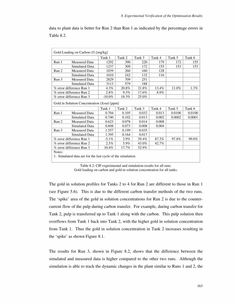
8. Experimental Verification of the Optimisation Results
163
data to plant data is better for Run 2 than Run 1 as indicated by the percentage errors in
Table 8.2.
Gold Loading on Carbon (Y) [mg/kg]
Tank 1 Tank 2 Tank 3 Tank 4 Tank 5 Tank 6 Run 1 Measured Data 1292 390 220 179 172 155 Simulated Data 1237 309 172 155 153 153 Run 2 Measured Data 1039 266 160 128 Simulated Data 1010 242 132 116 Run 3 Measured Data 2829 709 251 Simulated Data 3113 579 188 % error difference Run 1 4.3% 20.8% 21.8% 13.4% 11.0% 1.3% % error difference Run 2 2.8% 9.3% 17.6% 8.9% % error difference Run 3 -10.0% 18.3% 25.0%
Gold in Solution Concentration (Xout) [ppm] Tank 1 Tank 2 Tank 3 Tank 4 Tank 5 Tank 6 Run 1 Measured Data 0.704 0.105 0.032 0.013 0.0100 0.0100 Simulated Data 0.740 0.102 0.013 0.002 0.0002 0.0001 Run 2 Measured Data 0.623 0.078 0.014 0.008 Simulated Data 0.608 0.073 0.008 0.004 Run 3 Measured Data 1.557 0.199 0.035 Simulated Data 1.395 0.164 0.017 % error difference Run 1 -5.1% 2.9% 59.4% 87.2% 97.8% 99.0% % error difference Run 2 2.5% 5.9% 43.0% 42.7% % error difference Run 3 10.4% 17.7% 52.9% Notes: 1. Simulated data are for the last cycle of the simulation
Table 8.2: CIP experimental and simulation results for all runs. Gold loading on carbon and gold in solution concentration for all tanks.
The gold in solution profiles for Tanks 2 to 4 for Run 2 are different to those in Run 1
(see Figure 5.6). This is due to the different carbon transfer methods of the two runs.
The ‘spike’ area of the gold in solution concentrations for Run 2 is due to the counter-
current flow of the pulp during carbon transfer. For example, during carbon transfer for
Tank 2, pulp is transferred up to Tank 1 along with the carbon. This pulp solution then
overflows from Tank 1 back into Tank 2, with the higher gold in solution concentration
from Tank 1. Thus the gold in solution concentration in Tank 2 increases resulting in
the ‘spike’ as shown Figure 8.1.
The results for Run 3, shown in Figure 8.2, shows that the difference between the
simulated and measured data is higher compared to the other two runs. Although the
simulation is able to track the dynamic changes in the plant similar to Runs 1 and 2, the

8. Experimental Verification of the Optimisation Results
164
simulation under-predicts the measured data by 10% or greater. The only exception is
the gold loading on Tank 1 where it over-predicts.
0
500
1000
1500
2000
2500
3000
3500
0 12 24 36 48 60 72 84 96
Time [h]
Tank
1G
old
on C
arbo
n [m
g/kg
]
Simulation Actual
0
200
400
600
800
1000
0 12 24 36 48 60 72 84 96
Time [h]
Tank
2G
old
on C
arbo
n [m
g/kg
]
Simulation Actual
0
50
100
150
200
250
300
0 12 24 36 48 60 72 84 96
Time [h]
Tank
3G
old
on C
arbo
n [m
g/kg
]
Simulation Actual
0.0
0.5
1.0
1.5
2.0
0 12 24 36 48 60 72 84 96
Time [h]
Tank
1G
old
in S
olut
ion
[ppm
]
Simulation Actual
0.00
0.05
0.10
0.15
0.20
0.25
0.30
0.35
0 12 24 36 48 60 72 84 96
Time [h]
Tank
2G
old
in S
olut
ion
[ppm
]
Simulation Actual
0.00
0.02
0.04
0.06
0.08
0.10
0 12 24 36 48 60 72 84 96
Time [h]
Tank
3G
old
in S
olut
ion
[ppm
]
Simulation Actual Figure 8.2: Run 3 - Simulated and measured data for gold loading on carbon and gold in solution
concentration
The simulated gold loading on carbon for Tank 1 over-predicts its measured data by
10%. This error increases to 18% and 25% for Tanks 2 and 3 respectively. These
percentage errors for Tanks 2 and 3 are similar to those reported for Run 1 of 20-22%.
The large error of Tank 1 for Run 3, is not matched in Runs 1 and 2, where the errors
for the gold loading on the carbon are less than 5%. An accurate simulated value for the
gold loading on Tank 1 is more important than the other tanks as it is this value that
determines the gold revenue of the CIP plant. Hence the ability for a simulation model
to predict this value is important.
The errors for the gold in solution concentration ranges from 10% to 53%, representing
a 0.16ppm, 0.035ppm and 0.02ppm error for Tanks 1, 2 and 3 respectively. Again these
errors are higher than that reported for Runs 2 and 3.
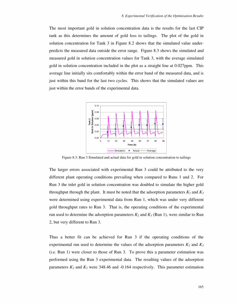
8. Experimental Verification of the Optimisation Results
165
The most important gold in solution concentration data is the results for the last CIP
tank as this determines the amount of gold loss to tailings. The plot of the gold in
solution concentration for Tank 3 in Figure 8.2 shows that the simulated value under-
predicts the measured data outside the error range. Figure 8.3 shows the simulated and
measured gold in solution concentration values for Tank 3, with the average simulated
gold in solution concentration included in the plot as a straight line at 0.027ppm. This
average line initially sits comfortably within the error band of the measured data, and is
just within this band for the last two cycles. This shows that the simulated values are
just within the error bands of the experimental data.
0.00
0.02
0.04
0.06
0.08
0.10
0 12 24 36 48 60 72 84 96
Time [h]
Tank
3G
old
in S
olu
tion
[ppm
]
Simulation Actual Average
Figure 8.3: Run 3 Simulated and actual data for gold in solution concentration to tailings
The larger errors associated with experimental Run 3 could be attributed to the very
different plant operating conditions prevailing when compared to Runs 1 and 2. For
Run 3 the inlet gold in solution concentration was doubled to simulate the higher gold
throughput through the plant. It must be noted that the adsorption parameters K2 and K3
were determined using experimental data from Run 1, which was under very different
gold throughput rates to Run 3. That is, the operating conditions of the experimental
run used to determine the adsorption parameters K2 and K3 (Run 1), were similar to Run
2, but very different to Run 3.
Thus a better fit can be achieved for Run 3 if the operating conditions of the
experimental run used to determine the values of the adsorption parameters K2 and K3
(i.e. Run 1) were closer to those of Run 3. To prove this a parameter estimation was
performed using the Run 3 experimental data. The resulting values of the adsorption
parameters K2 and K3 were 348.46 and -0.164 respectively. This parameter estimation

8. Experimental Verification of the Optimisation Results
166
is referred to as parameter estimation gEST 6-1 and its results, along with its statistical
data are listed in Table 8.3.
The K2 and K3 values of gEST 6-1 are very similar to those of gEST 5-3 of 351.19 and -
0.151 (gEST 5-3 was the parameter estimation run used that yielded the values of
adsorption parameters used in the model simulations). The objective function value for
gEST 6-1 of 263 is much lower than gEST 5-3 of 672. This lower value for gEST 6-1
is to be expected as there are three less tanks, and hence less experimental data for
gEST 6-1 compared to gEST 5-3. Therefore no conclusions can be drawn from the
lower objective function value.
gEST 6-1 Parameters Estimated: K2, K3 for Run 3 Results: K2 = 348.46 Objective Function = 263.11 K3 = -0.164 Statistical Data: Correlation between K2 and K3 = -0.997 t-test values at 95%: Reference Value = 1.665 K2 = 3.291 K3 = 3.927 95% Confidence Intervals: K2 = 348.46 ± 105.88 K3 = -0.164 ± 0.042
Table 8.3: Parameter Estimation gEST 6-1 Results - Estimating K2 and K3 using Run 3 data
The statistical data of the fit gEST 6-1 show that a satisfactory fit of the model is
achieved with t-values at 95% confidence of 3.3 and 3.9 for K2 and K3 respectively.
Both values are above the reference t-value of 1.65. The 95% confidence interval for K2
and K3 indicates that the values K2 and K3 can be rounded to 350 and -0.16 respectively.
These results are almost identical to the previous values of K2 and K3 of 350 and -0.15,
with the only difference being the K3 value. The gEST 6-1 K2 and K3 values were then
used to simulate experimental Run 3 again to determine whether a better fit of the
simulated to the measured data can be achieved and the results are shown in Figure 8.4
and Table 8.4.

8. Experimental Verification of the Optimisation Results
167
0
500
1000
1500
2000
2500
3000
3500
0 12 24 36 48 60 72 84 96
Time [h]
Tank
1G
old
on C
arbo
n [m
g/kg
]
Simulation Actual
0
200
400
600
800
1000
0 12 24 36 48 60 72 84 96
Time [h]
Tank
2G
old
on C
arbo
n [m
g/kg
]
Simulation Actual
0
50
100
150
200
250
300
0 12 24 36 48 60 72 84 96
Time [h]
Tank
3G
old
on C
arbo
n [m
g/kg
]
Simulation Actual
0.0
0.5
1.0
1.5
2.0
0 12 24 36 48 60 72 84 96
Time [h]
Tank
1G
old
in S
olut
ion
[ppm
]
Simulation Actual
0.00
0.05
0.10
0.15
0.20
0.25
0.30
0.35
0.40
0 12 24 36 48 60 72 84 96
Time [h]
Tank
2G
old
in S
olut
ion
[ppm
]
Simulation Actual
0.00
0.02
0.04
0.06
0.08
0.10
0 12 24 36 48 60 72 84 96
Time [h]
Tank
3G
old
in S
olut
ion
[ppm
]
Simulation Actual
Figure 8.4 Run 3 using gEST 6-1 results - Simulated and measured data for gold loading on carbon and gold in solution concentration
Gold Loading on Carbon (Y) [mg/kg] gEST 5-3 parameter values
K2 = 350, K3 = -0.15 gEST 6-1 parameter values
K2 = 350, K3 = -0.16 Tank 1 Tank 2 Tank 3 Tank 1 Tank 2 Tank 3 Measured Data 2829 709 251 2829 709 251 Simulated Data 3113 579 188 3111 608 195 % error difference -10.0% 18.3% 25.0% -10.0% 14.2% 22.3%
Gold in Solution Concentration (Xout) [ppm]
Tank 1 Tank 2 Tank 3 Tank 1 Tank 2 Tank 3 Measured Data 1.557 0.199 0.035 1.557 0.199 0.035 Simulated Data 1.395 0.164 0.017 1.487 0.186 0.020 % error difference 10.4% 17.7% 52.9% 4.5% 6.6% 43.8% Notes: 1. Simulated data are for the last cycle of the simulation
Table 8.4: CIP experimental and simulation results for Run 3 using gEST 5-3 and gEST 6-1 results Gold loading on carbon and gold in solution concentration for all tanks
The results show that overall, there is an improvement in the fit of simulated to
measured data. The results show that there is no change in the fit of the gold loading on
carbon for Tank 1, but there is an improvement in the fit of the gold loading on carbon

8. Experimental Verification of the Optimisation Results
168
for the other two tanks and for the gold in solution concentrations for all tanks. This is
reflected in the decrease in the percentage error difference for experimental Run 3
shown Table 8.4.
Table 8.4 shows the measured values for experimental Run 3 and simulated values
using both gEST 5-3 and gEST 6-1 parameter values. For the gold loading on carbon
for Tanks 2 and 3, the percentage error decreased by 3%, for the gold in solution
concentration for Tanks 1 and 2 the error decreased to 7% or less and for Tank 3 to 44%
at an absolute value of only 0.015ppm. These results confirm not only the sensitivity of
adsorption parameter K3 but also show that a better fit is always possible if the
parameter estimations are performed under the same operating conditions as the
experimental system.
Hence the simulation model clearly has a range of applicability of operating conditions.
This range is critically dependent on the values of the adsorption parameters, which was
highlighted by the work presented in Chapter 6, where the sensitivity of the model to
changes in model parameters was presented.
Another reason for the larger errors associated with the results of experimental Run 3
could be due to the partial carbon transfer used. Partial carbon transfer results in a
distribution of gold loadings on carbon. The simulation model calculates the gold
loading on carbon in each tank as an average gold loading across the carbon population
in the tank. The experimental data is obtained by analysing the gold content of the
sample of carbon. The sample size of the carbon collected is 3g. It is possible that the
sample of carbon collected for gold loading on carbon analysis is not large enough to be
representative of the average gold loading on the carbon across the carbon population,
leading to errors between the simulated and measured data.
Taking a larger sample size could affect the carbon population in the tanks and affect
the results in the experiment. The experiment assumes that the masses of carbon are
equal in all tanks. Using a larger carbon sample size could result in the lower tanks of
the CIP train containing more carbon than the tanks at the start of the CIP train. This is
also the reason duplicate samples were not taken.
8. Experimental Verification of the Optimisation Results
169
The gold balance calculations for Run 2 and 3 are shown in Appendix E. The gold
balance error for Runs 2 and 3 are 5.37% and 6.68%. These errors also represent the
errors associated with sampling analyses. Hence these error values confirm that
satisfactory sampling analysis techniques were used.
8.4 Analysis of the Objective Functions
The analysis of the objective function values for the experimental runs is divided into
four parts. Firstly the weighting factor applied to the objective function calculations is
described in Section 8.4.1. The objective function calculations for the simulated and
measured values are detailed in Section 8.4.2. The discussion of the results of the
objective function values for each run are presented in Section 8.4.3, and finally a
comparison of the objective functions for all three runs is performed in Section 8.4.4.
8.4.1 The Weighting Factor
The objective function was introduced in Chapter 7 and used to optimise the CIP pilot
plant. However the operating conditions used in the optimisation of the pilot plant are
different to those of the experimental runs due to practical restrictions in operating the
experimental apparatus. To aid in the comparison of the objective functions of the three
experimental runs and the work presented previously in Chapter 7, a weighting factor
was used. This weighting factor compensates each run for the actual amount of gold fed
into the pilot plant compared to the optimisation results. Thus the determination of the
objective function for the experimental runs comprises of two parts. The first involves
calculating the objective function value for one year’ s operation. Then this value is
weighted by multiplying it by a weighting factor.
The weighting factor is based on the gold throughput into the CIP pilot plant and is
shown in Equation (8.1)
)(
)(Factor Weighting
iRunAuoptAu= (8.1)

8. Experimental Verification of the Optimisation Results
170
where Au(opt) is the gold throughput of the CIP pilot plant for the optimisation work in
Chapter 7 in [mg Au/h], and Au(Runi) is the gold throughput for the experimental CIP
pilot plant Run i [mg Au/h]. The calculation of the weighting factors for all three
experimental runs is shown in Appendix K. The weighting factor for Runs 1, 2, and 3
are 2.589, 2.791 and 1.174 respectively. This factor compensates the objective function
for varying the gold throughput between the optimisation results and the experimental
operating conditions.
8.4.2 Objective Function Calculation
Two objective functions need to be calculated for each experimental run: the simulated
objective function determined by the simulation model and the actual or measured
objective function determined by the measured plant data collected during the
experimental run. These objective functions will be referred to as the simulated and
measured objective function.
The simulated objective function values were calculated from the data of the last cycle
of the run. These values were then used to determine the objective function for one
year’ s operation. It is this per annum value that is presented in the results. This process
is the same as that used for the optimisation work. These values were then combined
with the weighting factor to determine the weighted simulated objective functions. A
sample calculation for this is shown in Appendix K.
The (unweighted) measured objective function for the runs use the measured plant data.
The measured gold loading on carbon for Tank 1 and the gold in solution concentration
for the last tank (i.e. the gold in solution to tailings) are used in the calculation. Recall
from Section 7.2 the equation for the objective function is:
J = GoldRevenue – CapitalCostFn – TotVariableCost – GoldLost (8.2)
where J is the objective function, GoldRevenue is the amount of revenue generated by
the CIP plant, CapitalCostFn is the capital costs, TotVariableCost is the running costs,
and GoldLost is the cost of gold lost to tailings. All of the variables mentioned above
are in Australian Dollars. The CapitalCostFn and TotVariableCost are the same for

8. Experimental Verification of the Optimisation Results
171
both the simulated and measured objective functions. This is because the variables of
the capital and variable costs, which consist of the costs of the tanks, carbon transfer
pumps and the amount of carbon, are the same for both the simulated and measured
case.
The measured gold revenue is calculated based on the measured gold loading on carbon
for Tank 1, and the measured gold lost is calculated based on the measured gold in
solution concentration for the last tank of the CIP pilot plant. These unweighted
measured objective functions were then combined with the weighting factor to
determine the weighted objective function values. Table 8.5 and Table 8.6 list the
weighted simulated and measured objective function values of one year’ s operation for
all three experimental runs.
Run 1 Carousel carbon transfer
(1 pump)
Run 1 Carousel carbon transfer
(6 pumps)
Weighted Objective Function for Run 1 6 Tanks Pulp flow 8.18L/h @4.45ppm
Simulated [$] Measured [$] Simulated [$] Measured [$] Objective Function 5817.25 6240.16 5344.69 5767.59 Gold Revenue 7759.19 8197.64 7759.19 8197.64 Total Cost 1941.95 1957.48 2414.51 2430.05 - Capital Cost 959.22 959.22 1431.47 1431.47 - Variable Cost 982.68 982.68 983.00 983.00 - Gold Lost 0.04 15.58 0.04 15.58
Table 8.5: Run 1 - Weighted objective function for 1 and 6 carbon transfer pumps
Run 2 Sequential-pull carbon transfer
4 Tanks Pulp flow 8.16L/h @ 4.15ppm
Run 3 Sequential-pull carbon transfer
3 Tanks Pulp flow 8.18L/h @ 9.10ppm
Weighted Objective Function for Runs 2 and 3
Simulated [$] Measured [$] Simulated [$] Measured [$] Objective Function 5908.61 6055.36 8806.03 7756.29 Gold Revenue 7891.22 8048.37 10332.10 9301.18 Total Cost 1982.61 1993.01 1526.06 1544.89 - Capital Cost 918.12 918.12 673.57 673.57 - Variable Cost 1061.27 1061.27 833.23 833.23 - Gold Lost 3.22 13.62 19.26 38.09
Table 8.6: Runs 2 and 3 - Weighted objective function

8. Experimental Verification of the Optimisation Results
172
8.4.3 Objective Function Results
Table 8.5 shows the weighted simulated and measured objective function for Run 1.
Two scenarios are presented. The first is the ’true’ carousel method where only one
carbon transfer pump is included in the objective function calculations. The second
incorporates the costs of a pump for each tank, i.e. 6 carbon transfer pumps in total.
Both are presented to highlight the large differences in costs by adopting the carousel
method. In addition the costs for Run 1 with 6 pumps will be used later.
The simulated and measured objective function for Run 1 using only 1 pump are $5817
and $6240 respectively. The higher measured objective function is due to the higher
measured gold loadings on carbon recorded for Tank 1 of 1292mg/kg compared to its
simulated value of 1232mg/kg. The capital costs and variable costs are the same for
both the simulated and measured data. There is a large difference between the gold lost
values. This is due to the very low predicted gold in solution concentrations in Tank 6
compared to the measured values. Again it must be noted that is it difficult to detect
gold in solution concentrations lower than 0.01ppm and that this is the measured gold in
solution concentration to tailings for this run. The percentage difference between the
simulated and measured objective function is 6.5%, which indicates that the simulated
objective function is able to predict the measured objective function.
If all 6 pumps are included in the capital costs, then the simulated and measured
objective functions for Run 1 are $5345 and $5768 respectively. This represents a large
decrease in the value of the objective function when an additional 5 pumps are added to
the plant. This demonstrates the large savings that could be made if the carousel
method is used. However as stated in Section 7.4.1.1, the carousel method is not
commonly used in industry due to the additional operational difficulties it creates.
These additional operational aspects are not included in the current objective function.
Table 8.6 shows the objective function results for Run 2 and Run 3. The simulated and
measured objective functions for Run 2 are $5909 and $6055 respectively. Again the
difference between these two values is due to the differences in the simulated and
measured gold revenue and gold lost values as described earlier. The small percentage
difference in the simulated and measured objective function value of 2.5% confirms the

8. Experimental Verification of the Optimisation Results
173
simulation model’s ability to predict the measured behaviour. This is consistent with the
measured and simulated results of the gold loading on carbon and the gold in solution
concentration data presented earlier for Run 2.
The simulated and measured objective function results for Run 3 are also shown in
Table 8.6. These results are consistent with the gold loading on carbon and gold in
solution concentration results presented earlier, where the fit of simulated to measured
data for this run has the highest errors of all the experimental runs. The simulated and
measured objective functions for Run 3 are $8806 and $7756 respectively. The error
between the simulated and measured value is 10.9%. This error is mostly due to the
difference in the simulated and measured gold revenue values of $10332 and $9301
respectively. This in turn is due to the difference in the simulated and measured gold
loading on carbon for Tank 1. A comparison of the errors between the simulated and
measured objective function of 10.9% and the errors between the simulated and
measured gold loading on carbon for Tank 1 of 10% (see Table 8.2) confirms this
conclusion.
8.4.4 Comparison of all Experimental Runs
A comparison was performed on the objective function values of all three experimental
runs. However the runs do not use the same carbon transfer method. Experimental Run
1 used the carousel transfer method and Runs 2 and 3 used the sequential-pull method.
The major difference between the two methods, in relation to the objective function, is
the number of carbon transfer pumps used in the plant.
For sequential -pull method, each CIP tank has its own pump to transfer carbon, and for
the carousel method there is only one pump for the entire CIP circuit. This difference in
capital has a significant impact on the objective function value of the operation.
Therefore for the purposes of comparing the objective functions of the three
experimental runs, it will be assumed that each tank has its own pump to transfer the
carbon for all the runs. Thus an additional 5 pumps are added to the objective function
value for Run 1. Although Run 1 actually used the carousel method, which has been
shown to be more efficient than the sequential -pull, for the purpose of this analysis it
shall be assumed its results are reflective of the sequential -pull carbon transfer method.

8. Experimental Verification of the Optimisation Results
174
The optimisation work performed in Chapter 7 shows that, if given a CIP system
operating at 12h carbon cycle time, with 3, 4 or 6 tanks, the 3 tank system would result
in the highest objective function, followed by the 4 tank system and finally the 6 tank
system. It then follows that for the three experimental runs performed on the CIP pilot
plant, Run 3 (3 tanks) would have the highest objective function, followed by Run 2 (4
Tanks) and then Run 1 (6 tanks). This is confirmed in Figure 8.5 where the objective
function, gold revenue and total cost are plotted for both the simulated and measured
objective function values.
Simulated Objective Function
0
2000
4000
6000
8000
10000
12000
Run 1 - 6 Tanks Run 2 - 4 Tanks Run 3 - 3 Tanks
Experimental Run
[$/y
r]
Objective Function Gold Revenue Total Cost
Measured Objective Function
0
2000
4000
6000
8000
10000
12000
Run 1 - 6 Tanks Run 2 4 Tanks Run 3 3 Tanks
Experimental Run
[$/y
r]
Objective Function Gold Revenue Total Cost
Figure 8.5: Comparison of all three experimental runs
8.5 Conclusions
The experimental results presented in this chapter shows that the simulation model was
able to predict the measured data for Run 2, and to a lesser extent for Run 3. A
weighting factor was developed to enable the objective function of different
experimental runs to be compared against each other as well as with the optimisation
runs performed in Chapter 7. The simulated and measured objective function values
were calculated for each experimental run and the results show that the simulated results
were able to predict the experimental results for Runs 1 and 2, and to a lesser extent Run
3. Hence the objective function calculations have been tested and shown to be effective
in evaluating different operating conditions.

175
9. A Machine Learning Algorithm Application
An application of the CIP model is described. The model is used to generate
simulated plant data and subsequently used to develop an operational
classification model of the CIP process. Machine learning algorithms were
used to develop the classification model, which can be used to provide on-
line operator advice.
9.1 Introduction
The introduction of readily available computational power to process and store data
over the past 20 to 30 years has led to developments in the organisation and analysis of
such data to aid in business decision making. This process is often referred to as data
mining. Data mining is defined as the process of discovering patterns in data (Witten
and Frank, 2000). This process has been used in areas such as target marketing and risk
management where large databases of information are readily available. For example,
data mining is used in the banking sector to determine the credit risk of bank customers
(Cabena et al, 1997). Historical data of past customers are used to build a profile of a
good or bad new loan applicant and this profile can then be used to assess new loan
customers.
The applications of data mining are numerous in the business sector due to the ready
availability of data. However data mining has found little use in the mineral processing
sector due to the lack of reliable plant data.
This chapter will discuss the application of data mining techniques to data generated by
the CIP simulation model. Firstly a description of the types of data mining techniques
available will be provided in Section 9.2. Then the chosen data mining method will be
discussed using a simple example in Section 9.3. This method is then applied to the
CIP pilot plant described in Section 9.4.

9. A Machine Learning Algorithm Application
176
9.2 Data Mining Methods
Data mining, the analysis of data in databases, is performed through a computer
program that uses machine learning algorithms to derive decision structures from the
data. Witten and Frank (2000) identified four types of machine learning styles that can
be used to derive a decision model: classification learning, numerical prediction,
association learning and clustering.
Classification learning involves building a decision model to classify the data into pre-
defined classes. This decision model is sometimes referred to as a classification model.
Numerical prediction is similar to classification, however the decision model is used to
predict a numerical value instead of a class value. These two machine learning methods
are referred to as predictive modelling by Cabena et al (1997) as the resultant decision
model is used to predict a variable (either a class or numerical value) of interest.
Association learning involves searching for any associations between the different
attributes of the data. Clustering involves grouping the database into segments of
similar records. That is, the records share a number of common traits. This is also
known as segmentation.
The data mining technique that will be used in this work is classification learning. This
is described in more detail in the next section.
9.3 Classification Modelling
The purpose of developing a classification model is to provide a systematic approach to
classify given cases or instances, as described by a set of attributes, to one of several
available classes. Classification models can be built using two methods – one by using
the ‘human’ expert and the other by using historical data of the system (Quinlan, 1993).
The ‘human’ expert method involves interviewing personnel and those that are familiar
with the system to develop the model. This method can be very subjective and has been
utilised in the past to build knowledge-based systems.

9. A Machine Learning Algorithm Application
177
The second method involves the analysis and subsequent model development from data
of a system. Such a method removes the subjectivity from the data and takes advantage
of the mass of data generated by modern systems. For example the identity of a type of
organic plant may be identified by three attributes: its leaf size, stalk size and height.
This particular organic plant has three different species (or classes). Data can then be
collected for different plants by recording the leaf size, stalk size, height (i.e. its
attributes) and species class. This data can then be arranged in an appropriate file
format to use in appropriate software to build a classification model.
The construction of a classification model, performed by a computer program that uses
machine learning algorithms, examines data to determine if any patterns can be found.
It then generates a set of rules, also known as a decision tree, that can be used to classify
future cases. For the organic plant example, a classification model of the plant is
constructed to classify the plant into its correct species given the three known and
measured properties of the plant: its leaf size, stalk size and height. This example is a
simplified version of the Iris data set described by Witten and Frank (2000).
To analyse such data and develop the classification model a computer package Weka,
was used.
9.3.1 WEKA and C4.5
Weka was developed by the University of Waikato in New Zealand and stands for the
Waikato Environment for Knowledge Analysis (Witten and Frank, 2000). It is used to
apply a learning algorithm to a data set. Within its framework different types of
classification tools can be used to analyse a data set. For this application the learning
method used is C4.5 developed by Quinlan (1993) and the output is in the form of a
decision tree.
C4.5 is a set of computer programs that is used to constructs classification models by
finding patterns within data records (Quinlan, 1993). These programs are also known as
classifiers. There are limitations in the use of C4.5, and for it to be effective the data of
the system must lie within these limitations. These limitations are outlined by Quinlan
(1993):

9. A Machine Learning Algorithm Application
178
• Attribute-value description: The data that is used in the classification program is
made up of a set of instances or cases with each one representing one instance of the
system. Each instance is described by a fixed collection of properties or attributes.
The number and type of attributes must be the same for each case and its value must
be either numeric or discrete.
• Predefined classes: Each case is assigned to a class. This class must be determined
beforehand. In terms of machine learning, this is known as supervised machine
learning. Unsupervised learning is where the classes are determined by the
classifier.
• Discrete classes: Each class must be able to be easily distinguished from the other.
If a case is able to belong to two different classes it makes the development of the
classification model more difficult.
• Sufficient data: To be able to readily identify patterns in the data, a sufficient
amount of data is required. The amount of data will depend on factors such as the
number of attributes and classes used and the complexity of the model. The larger
the number of attributes and classes, and the greater the model complexity, more
data is required to construct a reliable model. The number of instances should be
significantly greater than the number of classes.
• “ Logical” classification models: The classification model developed is in the form
of a decision tree and an example of such a tree is shown in Figure 9.3. This limits
the ‘decisions’ to logical expressions of particular attributes.
To describe the application of classification modelling, an example shall be used. This
example, known as ‘The Weather Problem’ is a simple example used by Witten and
Frank (2000).
9.3.2 Classification Model Example - ‘The Weather Problem’
The weather problem consists of 12 independent instances or cases, which describe the
weather conditions of the day. The data set is presented in Table 9.1. The instances are
classified into two classes - whether one can play outside or not, based on the weather
conditions. Each instance is described by a set of attributes or properties and for this
example there are four attributes: outlook, temperature, humidity and windy. The
values of these attributes can be either numerical or discrete.

9. A Machine Learning Algorithm Application
179
For the data to be used in Weka it must be converted into a standard file format called
an ARFF file (Witten and Frank, 2000). The ARFF file for the weather data is shown in
Figure 9.1. The data is presented as a text file. Any line starting with the % sign are
comments. At the start of the file, the name of the file ‘weather’ is listed as relation,
then all the attributes are listed. For each attribute, its name is listed along with its type
of value enclosed in curly brackets. If the value is a numerical value, its type is ‘real’ .
For discrete values, values are listed in curly brackets. The final attribute ‘play’ is the
class value. After the list of the attributes, the data set is presented. Each instance is
presented in a single line with the values of its attributes listed in the same order as the
attributes list with commas separating the values.
Outlook Temperature [°F]
Humidity [%] Windy Play?
sunny 85 85 FALSE no sunny 80 90 TRUE no
overcast 83 86 FALSE yes rainy 70 96 FALSE yes rainy 68 80 FALSE yes rainy 65 70 TRUE no
overcast 64 65 TRUE yes sunny 72 95 FALSE no sunny 69 70 FALSE yes rainy 75 80 FALSE yes sunny 75 70 TRUE yes
overcast 72 90 TRUE yes overcast 81 75 FALSE yes
rainy 71 91 TRUE no
Table 9.1: The Weather Problem Data (Witten and Frank, 200)
%The Weather Problem%Witten and Frank, 2000
@relation weather
@attribute outlook {sunny, overcast, rainy}@attribute temperature real@attribute humidity real@attribute windy {TRUE, FALSE}@attribute play {yes, no}
@datasunny,85,85,FALSE,nosunny,80,90,TRUE,noovercast,83,86,FALSE,yesrainy,70,96,FALSE,yesrainy,68,80,FALSE,yesrainy,65,70,TRUE,noovercast,64,65,TRUE,yessunny,72,95,FALSE,nosunny,69,70,FALSE,yesrainy,75,80,FALSE,yessunny,75,70,TRUE,yesovercast,72,90,TRUE,yesovercast,81,75,FALSE,yesrainy,71,91,TRUE,no
Figure 9.1: ARFF file for the Weather Problem.

9. A Machine Learning Algorithm Application
180
Weka provides the classifier results in the form of a decision tree. For the simple
example, the output of Weka is shown in Figure 9.2. The results are divided into three
sections: the decision tree of the system as defined by C4.5, Weka’ s estimates of the
tree’ s predictive performance and the evaluation of data using stratified ten-fold cross-
validation. Each of these results will be discussed in further detail below.
%The Weather Problem%Witten and Frank, 2000
J48 pruned tree------------------
outlook = sunny| humidity <= 75: yes (2.0)| humidity > 75: no (3.0)outlook = overcast: yes (4.0)outlook = rainy| windy = TRUE: no (2.0)| windy = FALSE: yes (3.0)
Number of Leaves : 5
Size of the tree : 8
=== Error on training data ===
Correctly Classified Instances 14 100 %Incorrectly Classified Instances 0 0 %Kappa statistic 1Mean absolute error 0Root mean squared error 0Relative absolute error 0 %Root relative squared error 0 %Total Number of Instances 14
=== Confusion Matrix ===
a b <-- classified as 9 0 | a = yes 0 5 | b = no
=== Stratified cross-validation ===
Correctly Classified Instances 9 64.2857 %Incorrectly Classified Instances 5 35.7143 %Kappa statistic 0.186Mean absolute error 0.3036Root mean squared error 0.4813Relative absolute error 63.75 %Root relative squared error 97.5542 %Total Number of Instances 14
=== Confusion Matrix ===
a b <-- classified as 7 2 | a = yes 3 2 | b = no
Figure 9.2: Output of Weka for the Weather Problem
The decision tree is used to classify a case or instance of the system. The tree is made
of ‘leaves’ and ‘decision nodes’ . The leaves indicate the class and a decision node
represents a point in the tree where a test or decision is required to be made on an
attribute value. The sum of all the leaves and decision nodes is equal to the size of the
tree. For the Weather Problem example, the size of the decision tree is 8, consisting of
5 leaves and 3 decision nodes. In reading the decision tree, the classification process
starts at the ‘root’ of the tree, and moves to the first decision node to the attribute

9. A Machine Learning Algorithm Application
181
‘outlook’ . Then from this node, three paths can be taken depending on the ‘outlook’
value of the instance. Then the classification process moves to the next node until a leaf
is reached and the instance is classified. A more readable and graphical display of the
decision tree is shown in Figure 9.3.
Outlook
Yes
NoYes NoYes
WindyHumidity
≤75 >75 TrueFalse
Sunny Rainy
Overcast
Figure 9.3: Graphical display of the decision tree of the Weather Problem
Next to each leaf, a number in parentheses is shown. This number represents the
number of instances associated with this leaf. If there is a mis-classification by the leaf,
then the number of mis-classifications is also given.
The second part of the output, labelled ‘error on training data’ provides the estimates of
the predictive performance of the decision tree. The results show that the tree was able
to predict all cases. This is highly likely to be an over-prediction of the ability of the
tree to classify cases because the data set used to build the decision tree was also used to
predict the performance of the tree. These results are still useful as they generally
represent the upper bound of the tree’ s predictive performance (Witten and Frank,
2000). The results also list the class probabilities derived from the tree. The equations
for each of these statistical values are shown below.
Mean absolute error
n
apap nn −++− ...11 (9.1)
Root mean squared error
napap nn
2211 )(...)( −++−
(9.2)
Relative absolute error
aaaa
apap
n
nn
−++−−++−
...
...
1
11 (9.3)
9. A Machine Learning Algorithm Application
182
Root relative squared error 22
1
2211
)(...)()(...)(
aaaaapap
n
nn
−++−−++−
(9.4)
∑= ia
na
1 (9.5)
where p and a are the predicted and actual values respectively, n is the number of
instances, and i is the number of classes.
The confusion matrix shows how many instances have been classified in each class in
the form of a matrix. If all the instances have been assigned correctly, as in this case,
then the diagonal elements are non-zero numbers.
The third and final section of the output shows the results of a ‘stratified cross-
validation’ . This is a test that is performed on the data set and provides a better estimate
of the predictive performance of the decision tree.
In an ideal situation, to build a classification model, the data set would be divided into
three sets: a training, testing and validation set (Witten and Frank, 2000). The classifier
would use the training set to build the classification model, the model would then be
tested on the testing data set, and finally verified using the validation data set. Such a
process would ensure that the classification model has been rigorously tested and that
the same data set is not used for all three purposes. However in reality, such a process
is usually not achievable due to the limited amount of accurate data available. Thus
other forms of testing are used to determine the predictive performance of the data.
The testing method used by Weka in its C4.5 classification function is called the 10-fold
stratified cross-validation test. For this test, the data is firstly divided into ten equal
segments. Each segment is randomly sampled such that an equal proportion of each
class is represented. This procedure is called stratification. Then one segment is chosen
to be the testing data, and the rest is used as training data to build the decision tree. This
is performed ten times, once for each segment, i.e. it is cross-validated. The reason for
10-fold is that tests have been performed on a number of different datasets and different
learning techniques and it was found that ten is approximately the right number of folds
to obtain the best estimate of the error (Witten and Frank, 2000).
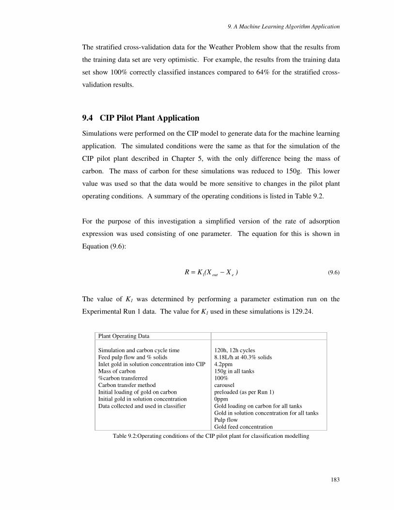
9. A Machine Learning Algorithm Application
183
The stratified cross-validation data for the Weather Problem show that the results from
the training data set are very optimistic. For example, the results from the training data
set show 100% correctly classified instances compared to 64% for the stratified cross-
validation results.
9.4 CIP Pilot Plant Application
Simulations were performed on the CIP model to generate data for the machine learning
application. The simulated conditions were the same as that for the simulation of the
CIP pilot plant described in Chapter 5, with the only difference being the mass of
carbon. The mass of carbon for these simulations was reduced to 150g. This lower
value was used so that the data would be more sensitive to changes in the pilot plant
operating conditions. A summary of the operating conditions is listed in Table 9.2.
For the purpose of this investigation a simplified version of the rate of adsorption
expression was used consisting of one parameter. The equation for this is shown in
Equation (9.6):
)X(XKR eout −= 1 (9.6)
The value of K1 was determined by performing a parameter estimation run on the
Experimental Run 1 data. The value for K1 used in these simulations is 129.24.
Plant Operating Data Simulation and carbon cycle time Feed pulp flow and % solids Inlet gold in solution concentration into CIP Mass of carbon %carbon transferred Carbon transfer method Initial loading of gold on carbon Initial gold in solution concentration Data collected and used in classifier
120h, 12h cycles 8.18L/h at 40.3% solids 4.2ppm 150g in all tanks 100% carousel preloaded (as per Run 1) 0ppm Gold loading on carbon for all tanks Gold in solution concentration for all tanks Pulp flow Gold feed concentration
Table 9.2:Operating conditions of the CIP pilot plant for classification modelling

9. A Machine Learning Algorithm Application
184
The simulations ran for a total of 120h (ten 12h carbon cycles) and data was recorded
for the point just before carbon transfer of the last carbon cycle of the simulation (as per
the optimisation and sensitivity analyses). The data was collected and used in the
classifier. Each simulation represented a single instance in the data set. The data used
were data that could be measured in a CIP plant. Thus the data used were the gold
loadings on the carbon and the gold in solution concentrations in all tanks, the amount
of gold in solution entering Tank 1, and the flow of pulp in the CIP plant. These are the
attributes of the data set.
Data was generated for changes in conditions that would be experienced in an
established gold plant. Variables that were changed were: the flowrate of the pulp,
representing fluctuations in the feed to the CIP system; the amount of gold in solution
entering Tank 1 (i.e. the gold in the ore of the plant), to resemble changes in the ore
body; and the efficiency of the adsorption process by changing the adsorption rate
parameter value K1. These three variables are referred to as the condition variables.
Two operating scenarios were used to build the data set. The first involved modelling
the CIP pilot plant where only one condition variable was changed at a time, i.e. only
the pulp flow, the gold in solution entering the CIP plant, or the adsorption parameter K1
was changed. This set of data is referred to as the single fault data set. The second data
set was created when two of the condition variables were changed at the same time, and
these are referred to as double fault data set. Each data set and its resultant
classification model are discussed in more detail and Sections 9.4.1 and 9.4.2.
9.4.1 Single Fault Classification Models
Three sets of simulations were performed to obtain data for the single fault data set, one
for each condition variable. A summary of these simulations is presented in Table 9.3.
For each simulation only one variable was changed at a time from its base value listed
in Table 9.2 yielding 112 instances or cases. Each simulation represented one instance
for the data set.
Firstly, 39 simulations were performed of varying pulp flow ranging from 2L/h to
40L/h. This range is based on the capacity of the equipment of the pilot plant. 45

9. A Machine Learning Algorithm Application
185
simulations were performed for a range of gold in solution concentrations of 1ppm to
17ppm which equates to a gold in ore value of 1.45g/t and 24.72g/t respectively, at a
leaching efficiency of 100%. Appendix L lists the equivalent values of gold in ore and
gold in solution concentration values. 28 simulations were performed for adsorption
parameter K1 with a range from 9 to 252.
Single Fault Simulations Simulation Set 1 - Varying Flow of Pulp Flow of Pulp ranged from 2 to 40L/h at 1h increments Total number of runs = 39 Simulation Set 2 - Vary Gold in Solution entering Tank 1 T1.Xin ranged from: 1 to 7ppm at 0.25ppm increments 7.5 to 17ppm at 0.5ppm increments Total number of runs = 45 Simulation Set 3 - Vary adsorption parameter K1 K1 ranged from 9 to 252 in increments of 9 Total number of runs = 28 Total runs for single fault simulations = 112
Table 9.3: Summary of single fault simulations
The data was collected and its class was assigned based on the conditions adopted. For
this data set two class conditions were used. The first had two classes – ‘normal’ and
‘not normal’ operating conditions. Normal operating conditions were defined as gold
loading on the carbon removed out of the system from Tank 1 to be greater than
1400mg/kg and the gold in solution out to tailings from Tank 6 had to be less that
0.005ppm. These values were based on the typical values in Australian gold plants
(Barbetti et al, 2000). Thus the ‘not normal’ conditions were defined as the fault
conditions of the plant.
The second classification condition had four classes: ‘normal’ , ‘bad flow’ , ‘bad carbon’
and ‘bad ore’ . Thus the ‘not normal’ class was subdivided into three fault classes. ‘Bad
flow’ represented pulp flow that was either too high or too low. ‘Bad carbon’
represented instances where the adsorption efficiency was too low (low K1 value). ‘Bad
ore’ represented ore that had either too little gold in the ore or too much gold for the
operating conditions of the plant.

9. A Machine Learning Algorithm Application
186
Two ARFF files were created and used in Weka to build the two classification models.
The results are shown in Figure 9.4 and Figure 9.5. Figure 9.4 shows the classification
results for the two classes classifier and is referred to as Classification Run 1, and
Figure 9.5 shows the results for the four classes classifier and is called Classification
Run 2.
J48 pruned tree------------------
T6.Xout <= 0.004921| T1.Y <= 1320.49: not_normal (12.0)| T1.Y > 1320.49: normal (54.0)T6.Xout > 0.004921: not_normal (46.0)
Number of Leaves : 3Size of the tree : 5
=== Error on training data ===
Correctly Classified Instances 112 100 %Incorrectly Classified Instances 0 0 %Kappa statistic 1Mean absolute error 0Root mean squared error 0Relative absolute error 0 %Root relative squared error 0 %Total Number of Instances 112
=== Confusion Matrix ===
a b <-- classified as 54 0 | a = normal 0 58 | b = not_normal
=== Stratified cross-validation ===
Correctly Classified Instances 111 99.1071 %Incorrectly Classified Instances 1 0.8929 %Kappa statistic 0.9821Mean absolute error 0.0089Root mean squared error 0.0945Relative absolute error 1.787 %Root relative squared error 18.8991 %Total Number of Instances 112
=== Confusion Matrix ===
a b <-- classified as 53 1 | a = normal 0 58 | b = not_normal
Figure 9.4: Classification Run 1 - results of single fault data set with two classes
The results show that Classification Run 1 has a smaller tree size of 5 compared to a
tree size of 11 for Classification Run 2. This is due to the smaller number of classes for
Classification Run 1. The prediction ability of both classification models is extremely
high with a stratified 10-fold cross-validation test value for the number of correctly
classified instances at 99% and 96% for Classification Run 1 and 2 respectively.

9. A Machine Learning Algorithm Application
187
The confusion matrix shows the mis-classified instances. For Classification Run 1, only
one instance was wrongly classified. The instance was classed as ‘not normal’ when it
was actually a ‘normal’ instance. For Classification Run 2, a total of four instances
were wrongly classified. One was classed as ‘bad ore’ but was actually ‘normal’ . The
other three were an instance of ‘bad flow’ , ‘bad ore’ , and ‘bad carbon’ which were
wrongly classified as ‘normal’ .
J48 pruned tree------------------
T1.Fpin <= 10| T6.Xout <= 0.004921| | T1.Y <= 1320.49| | | T1.Fpin <= 6: bad_flow (4.0)| | | T1.Fpin > 6: bad_ore (8.0)| | T1.Y > 1320.49: normal (54.0)| T6.Xout > 0.004921| | T1.Xin <= 9: bad_carbon (10.0)| | T1.Xin > 9: bad_ore (6.0)T1.Fpin > 10: bad_flow (30.0)
Number of Leaves : 6
Size of the tree : 11
=== Error on training data ===
Correctly Classified Instances 112 100 %Incorrectly Classified Instances 0 0 %Kappa statistic 1Mean absolute error 0Root mean squared error 0Relative absolute error 0 %Root relative squared error 0 %Total Number of Instances 112
=== Confusion Matrix ===
a b c d <-- classified as 54 0 0 0 | a = normal 0 34 0 0 | b = bad_flow 0 0 14 0 | c = bad_ore 0 0 0 10 | d = bad_carbon
=== Stratified cross-validation ===
Correctly Classified Instances 108 96.4286 %Incorrectly Classified Instances 4 3.5714 %Kappa statistic 0.9448Mean absolute error 0.0179Root mean squared error 0.1336Relative absolute error 5.4432 %Root relative squared error 33.0666 %Total Number of Instances 112
=== Confusion Matrix ===
a b c d <-- classified as 53 0 1 0 | a = normal 1 33 0 0 | b = bad_flow 1 0 13 0 | c = bad_ore 1 0 0 9 | d = bad_carbon
Figure 9.5: Classification Run 2 - results of single fault data set with four classes
Previous work on classification models by Werner et al (2002) found that normalised
data provided better results. Werner et al (2002) normalised the data by dividing the
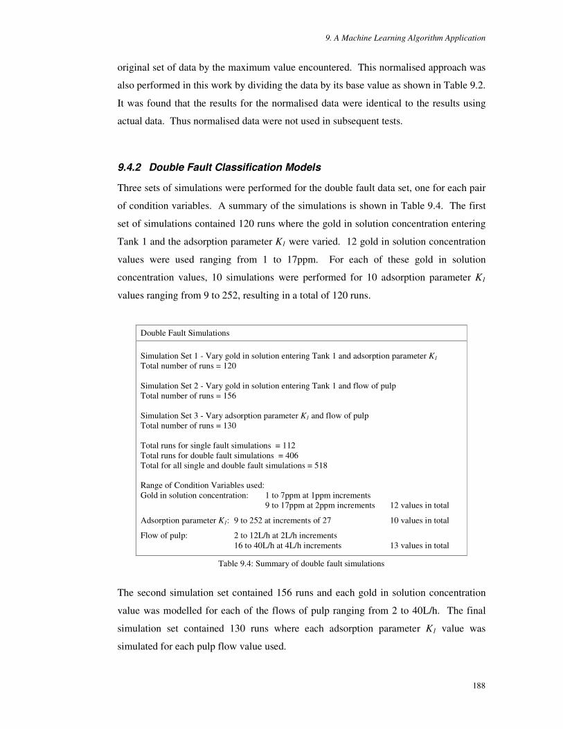
9. A Machine Learning Algorithm Application
188
original set of data by the maximum value encountered. This normalised approach was
also performed in this work by dividing the data by its base value as shown in Table 9.2.
It was found that the results for the normalised data were identical to the results using
actual data. Thus normalised data were not used in subsequent tests.
9.4.2 Double Fault Classification Models
Three sets of simulations were performed for the double fault data set, one for each pair
of condition variables. A summary of the simulations is shown in Table 9.4. The first
set of simulations contained 120 runs where the gold in solution concentration entering
Tank 1 and the adsorption parameter K1 were varied. 12 gold in solution concentration
values were used ranging from 1 to 17ppm. For each of these gold in solution
concentration values, 10 simulations were performed for 10 adsorption parameter K1
values ranging from 9 to 252, resulting in a total of 120 runs.
Double Fault Simulations
Simulation Set 1 - Vary gold in solution entering Tank 1 and adsorption parameter K1 Total number of runs = 120 Simulation Set 2 - Vary gold in solution entering Tank 1 and flow of pulp Total number of runs = 156 Simulation Set 3 - Vary adsorption parameter K1 and flow of pulp Total number of runs = 130 Total runs for single fault simulations = 112 Total runs for double fault simulations = 406 Total for all single and double fault simulations = 518 Range of Condition Variables used: Gold in solution concentration: 1 to 7ppm at 1ppm increments 9 to 17ppm at 2ppm increments 12 values in total
Adsorption parameter K1: 9 to 252 at increments of 27 10 values in total
Flow of pulp: 2 to 12L/h at 2L/h increments 16 to 40L/h at 4L/h increments 13 values in total
Table 9.4: Summary of double fault simulations
The second simulation set contained 156 runs and each gold in solution concentration
value was modelled for each of the flows of pulp ranging from 2 to 40L/h. The final
simulation set contained 130 runs where each adsorption parameter K1 value was
simulated for each pulp flow value used.

9. A Machine Learning Algorithm Application
189
A total of 406 simulations were performed to obtain data for the double fault conditions.
These simulations were classed into one of 7 class conditions, one ‘normal’ condition
and six fault conditions. Four of these conditions are the same as those used in
Classification Run 2. The other three classes are combinations of ‘bad flow’ , ‘bad ore’ ,
and ‘bad carbon’ that make up the double faults. They are ‘bad flow & bad ore’ , ‘bad
carbon & bad ore’ , and ‘bad flow & bad carbon’ . These 406 double fault cases were
combined with the 112 single fault cases for classification modelling. The results are
shown in Figure 9.6 and Figure 9.7 and is called Classification Run 3.
J48 pruned tree------------------
T6.Xout <= 0.004921| T1.Y <= 1320.77| | T1.Xin <= 2.75| | | T1.Fpin <= 5: bad_flow&bad_ore (4.0)| | | T1.Fpin > 5| | | | T6.Xout <= 0.001214: bad_ore (25.0)| | | | T6.Xout > 0.001214| | | | | T1.Fpin <= 9: bad_carbon&bad_ore (2.0)| | | | | T1.Fpin > 9: bad_ore (2.0/1.0)| | T1.Xin > 2.75| | | T6.Xout <= 0.000213| | | | T1.Fpin <= 2| | | | | T5.Xout <= 0.000063: bad_flow (14.0)| | | | | T5.Xout > 0.000063: bad_flow&bad_carbon (2.0)| | | | T1.Fpin > 2: bad_flow (12.0)| | | T6.Xout > 0.000213: bad_flow&bad_carbon (4.0/1.0)| T1.Y > 1320.77: normal (166.0)T6.Xout > 0.004921| T1.Fpin <= 10| | T1.Xin <= 13.5| | | T1.Xin <= 2.5: bad_carbon&bad_ore (6.0)| | | T1.Xin > 2.5| | | | T1.Fpin <= 9| | | | | T1.Fpin <= 5: bad_flow&bad_carbon (3.0)| | | | | T1.Fpin > 5| | | | | | T6.Xout <= 0.006836| | | | | | | T1.Xin <= 7.5: bad_carbon (3.0)| | | | | | | T1.Xin > 7.5: bad_carbon&bad_ore (2.0)| | | | | | T6.Xout > 0.006836: bad_carbon (45.0)| | | | T1.Fpin > 9| | | | | T1.Xin <= 5: bad_carbon (5.0/1.0)| | | | | T1.Xin > 5: bad_flow&bad_ore (5.0)| | T1.Xin > 13.5| | | T6.Y <= 146.125: bad_ore (12.0)| | | T6.Y > 146.125: bad_carbon&bad_ore (8.0)| T1.Fpin > 10| | T1.Xin <= 14| | | T1.Xin <= 2.5: bad_flow&bad_ore (14.0)| | | T1.Xin > 2.5| | | | T6.Xout <= 0.552978| | | | | T1.Xin <= 4: bad_flow (16.0)| | | | | T1.Xin > 4| | | | | | T1.Y <= 6826.29| | | | | | | T6.Xout <= 0.204397| | | | | | | | T1.Y <= 4567.09| | | | | | | | | T6.Y <= 169.024: bad_flow (19.0/1.0)| | | | | | | | | T6.Y > 169.024: bad_flow&bad_carbon (4.0)| | | | | | | | T1.Y > 4567.09: bad_flow (36.0)| | | | | | | T6.Xout > 0.204397: bad_flow&bad_carbon (6.0)| | | | | | T1.Y > 6826.29: bad_flow (52.0)| | | | T6.Xout > 0.552978| | | | | T1.Xin <= 5: bad_flow&bad_carbon (21.0)| | | | | T1.Xin > 5: bad_flow (14.0)| | T1.Xin > 14: bad_flow&bad_ore (16.0)
Number of Leaves : 28
Size of the tree : 55
Figure 9.6: Classification Run 3 - Decision tree for single and double faults data set with seven classes

9. A Machine Learning Algorithm Application
190
=== Error on training data ===
Correctly Classified Instances 514 99.2278 %Incorrectly Classified Instances 4 0.7722 %Kappa statistic 0.99Mean absolute error 0.0033Root mean squared error 0.0407Relative absolute error 1.5001 %Root relative squared error 12.257 %Total Number of Instances 518
=== Confusion Matrix ===
a b c d e f g <-- classified as 166 0 0 0 0 0 0 | a = normal 0 38 0 0 0 0 0 | b = bad_ore 0 0 52 0 0 0 0 | c = bad_carbon 0 0 0 162 0 0 0 | d = bad_flow 0 1 0 0 39 0 1 | e = bad_flow&bad_ore 0 0 0 0 0 18 0 | f = bad_carbon&bad_ore 0 0 1 1 0 0 39 | g = bad_flow&bad_carbon
=== Stratified cross-validation ===
Correctly Classified Instances 479 92.471 %Incorrectly Classified Instances 39 7.529 %Kappa statistic 0.9018Mean absolute error 0.0237Root mean squared error 0.1408Relative absolute error 10.7598 %Root relative squared error 42.4517 %Total Number of Instances 518
=== Confusion Matrix ===
a b c d e f g <-- classified as 165 1 0 0 0 0 0 | a = normal 0 35 0 0 0 2 1 | b = bad_ore 0 0 49 0 0 3 0 | c = bad_carbon 2 2 0 155 0 0 3 | d = bad_flow 0 1 3 0 36 0 1 | e = bad_flow&bad_ore 0 3 2 0 0 13 0 | f = bad_carbon&bad_ore 0 0 1 14 0 0 26 | g = bad_flow&bad_carbon
Figure 9.7: Classification Run 3 - Statistical data for single and double fault data set with seven classes
The results show a very large decision tree of a total size of 55 made up of 28 leaves
and 27 decision nodes. The 10-fold stratified cross-validation results show that 92% of
the instances were correctly classified. This is quite high given the complexity of the
decision tree.
The confusion matrix shows the breakdown of how the instances were classified. Of
the 39 mis-classified instances, only two instances were classed as ‘normal’ but were
actually a fault, and one ‘normal’ instance was classified as a fault. All the others were
mis-classifications within the six different fault classes. The mis-classifications occur
because the plant attributes for these faults are very similar. For example, if the plant
experiences high pulp flow or high gold ore grades, higher gold loadings on carbon and
higher losses to tailings will result. In addition two of the faults, ‘bad ore’ and ‘bad
flow’ are inter-related.

9. A Machine Learning Algorithm Application
191
‘Bad ore’ instances were created by changing the gold in solution concentration of gold
into the CIP system (T1.Xin). By changing this value, the total amount of gold entering
the CIP plant changes and directly affects the performance of the plant. ‘Bad flow’
instances were created by changing the pulp flowrate of the plant. Changes in pulp
flowrate also affect the total amount of gold entering the CIP plant. Thus an increase in
T1.Xin, pulp flowrate or an increase in both conditions, all lead to the same result, that
is, an increase in the total amount of gold entering the CIP plant in [mg/h]. This will
results in an increase gold loading on carbon and gold in solution concentrations in all
tanks. Thus the three fault conditions of ‘bad ore’ , ‘bad flow’ and ‘bad flow & bad ore’
are inter-related.
Therefore some of the mis-classification instances in the confusion matrix are a little
deceptive due to the inter-related properties of some of the faults as described above.
For example, two ‘bad flow’ instances were mis-classified as ‘bad ore’ and three as ‘bad
flow & bad carbon’ . However ‘bad flow’ is related to ‘bad ore’ , and ‘bad flow’ is also
one of the faults in ‘bad flow & bad carbon’ . Thus the operational impact of these mis-
classifications would not be severe.
The decision tree mis-classifies 39 instances out of a total of 518 instances, and only
two of these were wrongly classed as ‘normal’ when they are actually a fault. It is
better to have the classifier class a ‘normal’ instance as a fault rather than the reverse.
Thus the decision tree is able to identify that a fault does exist and is able to point the
user in the right direction to rectify the fault.
A complex decision tree is a common problem with classification models, in that they
have a tendency to overfit the training data. As a consequence they do not generalise
well to independent test sets, particularly those with noisy data (Witten and Frank,
2000). In addition such a complex tree is difficult to implement.
The complexity of the decision tree is due to the recursive partitioning method used in
C4.5 (Quinlan, 1993). This method continues to sub-divide the sets of training cases
until each subset contains cases of a single class or until no tests offer any improvement.
To minimise over-fitting, the concept of ‘pruning’ can be used. Pruning involves
eliminating sub-trees or branches of the decision tree with leaves, thus producing a less
9. A Machine Learning Algorithm Application
192
complex decision tree. This is done in C4.5 through reduced-error pruning. Reduced-
error pruning involves splitting the training data into two parts, using one part for
training or ‘growing’ the decision tree, and the other for pruning (Witten and Frank,
2000).
The data is split so that two-thirds of the instances are used for growing and the
remaining one-third used for pruning. The growing set is used to form a decision tree.
Then a part of the tree is removed and the pruning set is used on the new truncated tree
to see if it performs better than the original. This process continues until the tree cannot
be improved. The most important aspect of this procedure is that the training or
growing data is totally separate from the pruning set, and thus reduces the chances of
overfitting.
The main disadvantage of using such a process is whether there is enough data available
to split into the two training and pruning sets, and whether all the different types of
instances will be represented in both sets.
A new classification run, Classification Run 4, was performed on the single and double
fault data with two additional commands, the reduced-error pruning function was
enabled within Weka and the minimum leaf size was increased from 2 to 4 instances.
The results of this Run are shown in Figure 9.8. The size of the tree has halved from its
original size of 55 to 27.
The 10-fold stratified cross-validation results show that the correctly classified instances
decreased from 92.5% for Classification Run 3 to 87.8% due to reduced-error pruning.
This small decrease in the classifier’ s predictive ability resulted in a more simplified
decision tree that was half of its original size. Thus a more general decision tree is
produced. This is illustrated by following a branch for Classification Runs 3 and 4.
This is shown graphically in Figure 9.9.

9. A Machine Learning Algorithm Application
193
J48 pruned tree------------------
T6.Xout <= 0.004921| T1.Y <= 1320.77| | T1.Xin <= 2.5: bad_ore (23.0/6.0)| | T1.Xin > 2.5: bad_flow (24.0/5.0)| T1.Y > 1320.77: normal (111.0)T6.Xout > 0.004921| T1.Fpin <= 10| | T1.Xin <= 13.5| | | T1.Xin <= 2.5: bad_carbon&bad_ore (5.0)| | | T1.Xin > 2.5: bad_carbon (42.0/7.0)| | T1.Xin > 13.5| | | T6.Y <= 147.103: bad_ore (8.0)| | | T6.Y > 147.103: bad_carbon&bad_ore (4.0)| T1.Fpin > 10| | T1.Xin <= 14| | | T1.Xin <= 2.5: bad_flow&bad_ore (8.0)| | | T1.Xin > 2.5| | | | T6.Xout <= 0.552978| | | | | T1.Y <= 6087.24| | | | | | T2.Xout <= 1.44509: bad_flow (36.0/2.0)| | | | | | T2.Xout > 1.44509: bad_flow&bad_carbon (5.0)| | | | | T1.Y > 6087.24: bad_flow (46.0)| | | | T6.Xout > 0.552978| | | | | T1.Xin <= 5: bad_flow&bad_carbon (14.0)| | | | | T1.Xin > 5: bad_flow (9.0)| | T1.Xin > 14: bad_flow&bad_ore (11.0)
Number of Leaves : 14
Size of the tree : 27
=== Error on training data ===
Correctly Classified Instances 487 94.0154 %Incorrectly Classified Instances 31 5.9846 %Kappa statistic 0.9217Mean absolute error 0.0285Root mean squared error 0.1223Relative absolute error 12.9361 %Root relative squared error 36.8743 %Total Number of Instances 518
=== Confusion Matrix ===
a b c d e f g <-- classified as 166 0 0 0 0 0 0 | a = normal 0 37 0 1 0 0 0 | b = bad_ore 0 0 52 0 0 0 0 | c = bad_carbon 0 0 0 162 0 0 0 | d = bad_flow 0 5 5 1 30 0 0 | e = bad_flow&bad_ore 0 3 2 0 0 13 0 | f = bad_carbon&bad_ore 0 0 4 10 0 0 27 | g = bad_flow&bad_carbon
=== Stratified cross-validation ===
Correctly Classified Instances 455 87.8378 %Incorrectly Classified Instances 63 12.1622 %Kappa statistic 0.8407Mean absolute error 0.0464Root mean squared error 0.1736Relative absolute error 21.0651 %Root relative squared error 52.3303 %Total Number of Instances 518
=== Confusion Matrix ===
a b c d e f g <-- classified as 163 2 1 0 0 0 0 | a = normal 1 34 0 0 0 3 0 | b = bad_ore 0 0 48 0 3 1 0 | c = bad_carbon 2 3 0 154 0 0 3 | d = bad_flow 0 3 5 3 30 0 0 | e = bad_flow&bad_ore 0 5 6 0 0 7 0 | f = bad_carbon&bad_ore 0 0 4 18 0 0 19 | g = bad_flow&bad_carbon
Figure 9.8: Classification Run 4 - Results of single and double fault data set with seven classes using
reduced-error pruning

9. A Machine Learning Algorithm Application
194
T6.Xout≤ 0.0049ppm
T1.XinNormal
T1.Y> 1321mg/kg ≤ 1321mg/kg
FpulpT6.Xout
>2.75ppm ≤ 2.75ppm
Bad ore &bad flow
T6.Xout
>5L/h ≤ 5L/h
Bad oreFpulp
>0.001ppm ≤ 0.001ppm
Bad ore &bad carbon
Bad ore
>9L/h ≤ 9L/h
Bad flow &bad carbon
Fpulp
≤ 0.0002ppm > 0.0002ppm
Bad flowT5.Xout
≤ 2L/h
Bad flowBad flow & badcarbon
≤ 0.000063ppm
> 2L/h
> 0.000063ppm
T6.Xout≤ 0.0049ppm
T1.XinNormal
T1.Y> 1321mg/kg ≤ 1321mg/kg
Bad oreBad flow
>2.5ppm ≤ 2.5ppm
Classification Run 4
Classification Run 3
Figure 9.9: T6.Xout ��������SSP�EUDQFK�IRU�&ODVVLILFDWLRQ�5XQV���DQG��
Figure 9.9 shows a partial decision tree of the (T6.Xout �� ������SSP��SDWK� IRU� ERWK�Classification Runs 3 and 4. Classification Run 3 has 9 leaves and Classification Run 4
only has 3. All 7 classes are utilised for the branch in Classification 3. Only 3 classes
are used in Classification Run 4 and they are ‘normal’ , ‘bad ore’ and ‘bad flow’ .

9. A Machine Learning Algorithm Application
195
The path to the ‘normal class’ is the same for both runs. The path to ‘bad ore’ for
Classification Run 4 is further divided into 4 streams with 3 classes in Classification
Run 3. These classes are the 3 different combinations of ‘bad ore’ , i.e. ‘bad ore’ , ‘bad
ore & bad carbon’ , and ‘bad ore & bad flow’ . Thus the different combinations of ‘bad
ore’ in Classification Run 3 have been grouped into a single ‘bad ore’ class in Run 4.
This makes the Run 4 decision tree less complex. This pattern of behaviour is the same
for the ‘bad flow’ class for Classification Run 4. This path is further divided into 4
paths for Classification Run 3 leading to one of the ‘bad flow’ class combinations.
This analysis of a branch of Classification Runs 3 and 4 shows that the reduced-error
pruning does lead to a less complex and more general decision tree. However pruning
will result in a larger number of mis-classifications. The decision trees of these two
classification runs show that the total number of mis-classifications in the (T6.Xout ��0.0049ppm) path is 2 for Classification Run 3 and 11 for Classification Run 4. Hence
there is a trade off for a less complex tree and larger classification errors.
9.5 Conclusions
The CIP model developed in this work was used to produce simulated plant data to
build a classification model of the process. This classification model could be used by
operators to diagnose operating faults in the CIP process. Such a comprehensive set of
plant data could not be obtained from sampling campaigns as it would not be possible to
subject a full scale plant to a wide range of operating conditions.
This chapter only obtained data by changing three control variables: the flow of pulp
through the CIP plant, the gold in solution concentration entering the plant and the
adsorption capacity of the carbon; to illustrate the application of using machine learning
algorithms. Additional control variables can be added to this pool, such as the mass of
carbon and type of carbon transfer employed, to build a larger database of conditions of
the CIP plant. Such a database could be used to form the basis of a better understanding
of the CIP process and used for personnel training purposes.

196
10. Conclusions and Further Work
10.1 Conclusions
A simulation model of the CIP process has been developed and verified using a small
scale CIP pilot plant. This was used instead of real plant data due to the benefits of
being able to control and accurately measure every aspect of the CIP pilot plant.
The model was based on simple film-diffusion mass transfer with a Freundlich
equilibrium isotherm to describe the equilibrium between the gold in solution and gold
adsorbed onto carbon. The equilibrium isotherm parameter values were determined
through a series of laboratory equilibrium tests, and the adsorption rate parameters were
determined using data from the first experimental run of the CIP pilot plant. The model
was then verified by a further independent experimental test. The results of the
simulation model were in good agreement with the plant data.
Sensitivity analyses were performed on the model parameters. It was found that the
gold loadings on carbon and the gold in solution concentration for all the tanks were not
sensitive to changes in Freundlich isotherm parameter b. Changes in Freundlich
isotherm parameter A, and the adsorption rate parameters K2 and K3 had little effect on
the gold loading on carbon for Tank 1, but did affect the gold loading on carbon for all
other tanks and the gold in solution concentrations.
An objective function was developed based on the revenue and costs of the CIP process.
This function was used to investigate the following:
• Optimise the operations of the CIP pilot plant based on the number of tanks in the
CIP process, the volume of the tanks, the carbon cycle time and the mass of carbon
in the tanks.
• Different carbon management strategies. A total of 17 strategies were investigated.
• The proposal of adding new carbon into the CIP process in other tanks as well as the
final tanks. It was found that such a proposal did not improve the operations of the
CIP plant.

10. Conclusions and Further Work
197
• The proposal of recirculating a portion of the tailings solution back into the CIP
plant. It was found that this proposal did not improve the operations of the plant.
The objective function costings of the CIP plant were compared with published industry
costings. It was found that the costs developed fell within the published range. Thus
the objective function can be used to evaluate the performance of any CIP plant from a
small scale laboratory plant to a full scale gold plant.
Two additional experimental runs were performed to verify the simulation model and
the objective function developed. The operating conditions of the experimental runs
were based on the optimisation results of the CIP plant. The results show that the
simulation model was able to predict the measured data for one of the experimental runs
and to a lesser extent, the second run.
The CIP model was also used to produce plant data under various operating conditions.
This data was used to build a classification model of the CIP process using machine
learning algorithms. This demonstrated a further use of the simulation model.
In summary the major contributions of this work are:
• The development of a simulation model that has been verified with reliable plant
data.
• The development of an objective function of the CIP plant that can be used to
evaluate the performance of any CIP plant from a small scale laboratory plant to a
full scale gold plant.
• The investigation of 17 different carbon management strategies. It was found that
the best strategy was the carousel method. The best sequential carbon transfer
method was a modified sequential pull method where carbon is firstly removed from
Tank 1 to elution, then carbon is moved from Tank 6 to 5, new carbon is added to
Tank 6, and then carbon is ‘pulled’ up the tank train by transferring carbon from
Tank 2 to 1, Tank 3 to 2, Tank 4 to 3, and finally Tank 5 to 4.
• The proposal of recirculating a portion of the tailings solution back into the CIP
process was investigated. It was found that this did not improve the performance of
the CIP plant.

10. Conclusions and Further Work
198
• The proposal of adding a portion of new carbon into the CIP plant in other tanks as
well as the final tank was investigated. It was found that this did not improve the
performance of the CIP plant.
• The model was used to produce simulated plant data to build a classification model
of the process.
10.2 Recommendations for Further Work
During the course of this research, the following areas have been identified as worthy of
further investigation:
• Include an ‘operational difficulty’ function in the value of the objective function.
Such a function would then take into account the additional operating difficulties of
the carousel carbon transfer method over other methods. This would then provide a
more realistic objective function of the carousel carbon transfer method.
• Labour intensive methods were used to transfer carbon in the three experimental
runs on the CIP pilot plant performed in this work. This approach was taken to
ensure an accurate measurement of carbon was obtained. In addition, a greater
understanding of the behaviour of the carbon has been gained. With this additional
knowledge, the airlifts should be utilised in future experimental work on the CIP
pilot plant. This approach would not only be less labour intensive, but it would also
be more realistic in mimicking a full scale gold plant.
• The data mining application presented could be extended further by generating more
data. In addition, other control variables could be added such as carbon mass,
carbon cycle time, and the carbon transfer method. This data set could then be
divided into three separate sets with each set being used for testing, training and
verification. This would ensure that the decision tree is tested with data that has not
been used for training.
• This classification model and its database could be used to form the basis of a better
understanding of the CIP process. It could also be used by operators to diagnose
operating faults in the CIP process, used for training purposes, or be incorporated as
an on-line tool.
• Investigate the effectiveness of other data mining packages for this data set.

10. Conclusions and Further Work
199
• Incorporate the model into a plant wide model of the gold process. This model
could be used to generate data for machine learning algorithms. Such as data set
could be used to develop an on-line tool for the entire plant.
• Add leaching kinetics to the model and extend it to cover both leaching and
adsorption. The testing and verification of this model could be performed on the
current CIP pilot plant as a CIL process. Alternately, the leaching train of the CIP
pilot plant (which was not utilised in this work) could be used with the current
adsorption train.
• Carbon management strategies of a full scale plant can be investigated on the pilot
plant. The pilot plant could be operated in parallel with an existing gold plant by
using the pulp feed straight from the plant. This would enable various operating
strategies to be tested using the same ore throughput as the plant without any
disruptions to gold production.
• Perform CIP plant optimisation using the mixed-integer nonlinear programming
technique so that continuous decision variables such as carbon cycle time, and the
discrete (integer) decision variables, such as number of tanks and the carbon transfer
modes can be optimised simultaneously.
• Perform additional pilot plant experiments to verify the abnormal operations and
scenarios simulated in the Data Mining Section in Chapter 9.
• The classification model used in Chapter 9 is deterministic. A more realistic model
that is more susceptive to sensor noises and process disturbances, such as a
probability based classification model (such as Bayesian Network ) could be used.

200
Nomenclature
A, b Isotherm parameters Ac Surface area of carbon [m²/kg] AnnualRate Percentage of capital cost to be recovered per year Au(opt) Gold throughput for optimisation simulations [mg/h] Au(Runi) Gold throughput for the experimental Run i [mg/h] C Carbon content [g/L] C00h Carbon content [g/L] C1T % carbon transferred [%] CapitalCostFn Function for the capital cost of the CIP plant [$] CarbonCost Cost of activated carbon [$/kg] CarbonInTime Time required to put new carbon into CIP plant [h] CarbonLoss Fraction of carbon lost per year [%] CarbonLossCost Cost of carbon loss to carbon attrition [$] CPF Pulp flowrate of carbon transfer pump [L/h] ElutionCost1 Elution cost function variable ElutionCost2 Elution cost function variable FCin Mass flow of carbon into the tank [kg/h] FCout Mass flow of carbon out of the tank [kg/h] g Acceleration due to gravity [m/s²] GoldLost Cost of gold lost to tailings [$] GoldPrice Price of gold [$/g] GoldRevenue Revenue generated from the CIP plant [$] i ith tank J Objective function [$] k kn model parameter k1, k2 Nicol Model rate constants K1, K2, K3 Adsorption rate parameters ka, kd Dixon model parameters kf Film mass transfer coefficient [kg/m²/h] Mc Mass of carbon [kg] MFs Mass flow of solution [kg/h] Msoln Mass of solution in the tank [kg] n kn model parameter N Number of tanks PowerCost Cost of electrical power [kWh] PulpSoln Mass flow rate of solution through the CIP process [kg/h] PumpCapCost1 Pump cost function variable PumpCapCost2 Pump cost function variable

201
PumpCapCost3 Pump cost function variable PumpEff Efficiency rating of pump PumpHead Head of carbon transfer pump [m] PumpPower Power rating of carbon transfer pump [kW] R Rate of gold adsorption onto carbon [mg/kg/h] RecircSoln Mass flow of the recirculated pulp solution [kg/h] SGpulp Specific gravity of pulp [kg/L] t Time [h] TankCost1 Tank cost function variable TankCost2 Tank cost function variable TankCost3 Tank cost function variable TotalCost Total costs of the CIP plant [$] TotCapitalCost Total costs of all capital equipment in CIP plant [$] TotCarbonCost Cost of activated carbon [$] TotElutionCost Cost of eluting carbon [$] TotPumpCapCost Cost of carbon transfer pump [$] TotPumpVarCost Operating costs of the carbon transfer pump [$] TotTankCost Cost of CIP tanks [$] TotVariableCost Total costs of elution, pump power and carbon loss [$] TransferTime Time required to transfer carbon from Tank i [h] V Volume of tank [m³] Weighting Factor Ratio of gold feed in optimisation and experimental runs x, Xout Gold in solution concentration in the tank & leaving the tank [ppm] xe, Xe Equilibrium gold in solution concentration [ppm] Xin Gold in solution concentration entering the tank [ppm] xss Steady state concentration of gold in solution [ppm] y, Y Gold loading on carbon in the tank & leaving the tank [mg/kg] y0 Initial gold loading on carbon [mg/kg] or [g/t] ye, Ye Equilibrium gold loading on carbon [mg/kg] Yin Gold loading on carbon entering the tank [mg/kg]
recirculating tailings pulp flow fraction

202
References
1. Adams, M.D. (1990a) ‘The chemical behaviour of cyanide in the extraction of gold. 1. Kinetics of cyanide loss in the presence and absence of activated carbon’ Journal of the South African Institute of Mining and Metallurgy, Vol. 90, No. 2, pp. 37-44.
2. Adams, M.D. (1990b) ‘The chemical behaviour of cyanide in the extraction of gold. 2. Mechanisms of cyanide loss in the carbon-in-pulp process’ Journal of the South African Institute of Mining and Metallurgy, Vol. 90, No. 3, pp. 67-73.
3. Ahmed, F.E., Young, B.D., Bryson, A.W. (1992) ‘Comparison and modelling of the adsorption kinetics of gold cyanide onto activated carbon and resin in a silica slurry’ Hydrometallurgy, Vol. 30, pp. 257-275.
4. Aldrich, C., Van Deventer, J.S.J, Reuter, M.A. (1994) ‘The application of neural nets in the metallurgical industry’ Minerals Engineering, Vol. 7, No. 5/6, pp. 793-809.
5. Aldrich, C., Van Deventer, J.S.J, Van der Walt, T.J., Reuter,M.A. (1993) ‘Recent advances in the simulation of mineral processing circuits using artificial intelligence’ Proceedings of the XVIII International Mineral Processing Congress, Sydney, May 23-28, Vol. 2, pp. 529-537.
6. Annandale, G.J., Lorenzen, L., Van Deventer, J.S.J, Aldrich, C. (1996) ‘Neural net analysis of the liberation of gold using diagnostic leaching data’ Minerals Engineering, Vol. 9, No. 2, pp. 195-213.
7. Barbetti, K., O’ Leary, S., Staunton, W (2000) ‘A Review of the AMIRA P420A Gold Industry Survey’ AMIRA Project P420A - Gold Processing Technology, Module 2: Best Practice/Benchmarking Report’ , January 2000.
8. Bromby, Robin (2002) ‘Mining business worth its weight in gold’ The Weekend Australian, August 17-18, pp. 18.
9. Cabena, P., Hadjinian, P., Stadler, R., Verhees, J., Zanasi, A. (1997) Discovering Data Mining From Concept to Implementation, Prentice Hall PTR, New Jersey.
10. Carrier, C., Hodouin, D., Courchesne, M. (1987) ‘Dynamic simulation of the CIP gold recovery process’ , Proceedings of the International Symposium on Gold Metallurgy, Winnipeg, August 23-26, Vol. 1, pp. 309-325.
11. Cho, E.H. and Pitt, C.H. (1979) ‘Kinetics and thermodynamics of silver cyanide adsorption on activated charcoal’ Metallurgical Transactions B (Process Metallurgy) June, Vol. 10B, No. 2, pp. 165-169.
12. Cho, E.H., Nixon, S.N., Pitt, C.H. (1979) ‘The kinetics of gold cyanide adsorption on activated charcoal’ Metallurgical Transactions B (Process Metallurgy) June, Vol. 10B, No. 2, pp. 185-189.
13. Coetzee, J.W. and Gray, D.E. (1999) ‘Counter-current vs co-current flow in carbon-in-pulp adsorption circuits’ Minerals Engineering, Vol. 12, No. 4, pp. 415-422.

203
14. Dixon, S., Cho, E.H., Pitt, C.H. (1978) ‘The interaction between gold cyanide, silver cyanide and high surface area charcoal’ AIChE Symposium Series 74, vol. 74, No. 173, pp. 75-83.
15. Draper, N.R., Smith, H. (1981) Applied Regression Analysis, John Wiley and Sons, Canada, pp. 95, 487-388.
16. Fleming, C., Nicol, M.J., Nicol, D.I. (1908) ‘The optimisation of a carbon-in-pulp adsorption circuit based on the kinetics of extraction of aurocyanide by activated carbon’ Presented at Mintek meeting ‘Ion Exchange and Solvent Extraction in Meineral Processing’ , Randburg, Mintek, February.
17. Fleming, C.A., Nicol, M.J. (1984) ‘The absorption of gold cyanide onto activated carbon. 3. Factors influencing the rate of loading and the quilibrium capacity’ Journal of the South African Institute of Mining and Metallurgy, Vol. 84, No. 4, pp. 85-93.
18. Gliese, R., Petter, C.O., Sampaio, C.H. (1997) ‘The simulation of CIP and CIL processing using carbon loading population balance’ Proceedings of the XX International Mineral Processing Congress, Aachen, Sept. 21-26.
19. Groth, Robert (1997) Data Mining A Hands-On Approach for Business Professionals, Prentice Hall PTR, New Jersey.
20. Hangos, K.M., Cameron, I.T. (2001) Process Modelling and Analysis, Academic Press, XX, pp21.
21. Kalgoorlie Consolidated Gold Mines Fimiston Gold Plant Flow Sheet,1999 [Online, accessed 8 Nov. 1999] URL: http://www.kalgold.com.au/image/fc_Fim.gif.
22. Kiranoudis, C.T.,. Maroulis, Z.B.,Papassiopi, N., and Paspaliaris, I. (1998) ‘Modelling and optimization of carbon-in-pulp gold recovery processes’ IMA Journal of Mathematics Applied in Business and Industry, Vol. 9, No. 1, pp. 35-54.
23. Le Roux, J.D., A.W. Bryson, B.D. Young, (1991) ‘A comparison of several kinetic models for the adsorption of gold cyanide onto activated carbon’ J. S. Afr. Inst. Min. Metall., Mar., vol 91, No. 3, pp. 95-103.
24. Liebenberg, S.P., Van Deventer, J.S.J (1998) ‘The quantification of shifting adsorption equilibria of gold and base metals in CIP plants’ Minerals Engineering, Vol. 11, No. 6, pp. 551-562.
25. Lightnin ‘Labmaster SI Mixers - Operational Guide’ , 1994.
26. Lui, G.Q., Yen, W.T. (1995) ‘Dissolution kinetics and carbon adsorption for the cyanidation of gold ores in oxygen-enriched slurry’ CIM Bulletin, Vol. 88, No. 986, pp. 42-48.
27. Lynch, A.J., Morrison, R.D. (1999) ‘Simulation in mineral processing - history, present status and possibilities’ , Journal of the South African Institute of Mining and Metallurgy, Vol. 99, No. 6, pp. 283-288.
28. Marlin, Thomas E. (1995) Process Control: Designing Processes and Control Systems for Dynamic Performance. McGraw-Hill, Singapore, pp. 382-386.

204
29. Marsden, J., House, I. (1992) The Chemistry of Gold Extraction, Ellis Horwood Ltd, England.
30. Mehrotra, K., Mohan, C.K., Ranka, S. (1997) Elements of artificial neural networks, MIT Press, USA.
31. Nicol, M.J., Fleming, C.A. & G. Cromberge, G (1984a) ‘The absorption of gold cyanide onto activated carbon. 1. The kinetics of absorption from pulps’ Journal of the South African Institute of Mining and Metallurgy, Vol. 84, No. 2, pp. 50-54.
32. Nicol, M.J., Fleming, C.A. & G. Cromberge, G (1984b) ‘The absorption of gold cyanide onto activated carbon. 2. Application of the kinetic model to multistage absorption circuits’ Journal of the South African Institute of Mining and Metallurgy, Vol. 84, No. 3, pp. 70-78.
33. O’ Leary, S., Staunton, W (1999) ‘A Review of the Elution/Electrowinning Survey of Sponsors Sites’ AMIRA Project P420A - Gold Processing Technology, Module 2: Best Practice/Benchmarking, April.
34. O’ Leary, S., Staunton, W (2000) ‘A Review of the Carbon Management of Sponsors Sites’ AMIRA Project P420A - Gold Processing Technology, Module 2: Best Practice/Benchmarking, Module 4: Carbon Management, June.
35. Petersen, F.W. (1997) ‘The characterisation of the pregrobbing phenomenon during gold extraction’ Proceedings of the XX International Mineral Processing Congress, Aachen, Sept. 21-26.
36. Petersen, K.R.P., Lorenzen, L. (1997) ‘Gold liberation modelling using neural network analysis of diagnostic leaching data’ Proceedings of the XX International Mineral Processing Congress, Aachen, Sept. 21-26, Vol. 1, pp391-400.
37. Pleysier, Ron (1998) AMIRA P420A Report ‘Commissioning of the CIP/CIL Mini Rig’ .
38. Process Systems Enterprise Ltd (1999) gPROMS Introductory User’ s Guide, Release 1.7, May.
39. Process Systems Enterprise Ltd (2001) gPROMS Advanced User’ s Guide, Release 2.0, 14 May.
40. Quinlan, J. Ross (1993) C4.5 : Programs for Machine Learning, Morgan Kaufmann, California, USA.
41. Rees, K.L, Van Deventer, J.S.J (2001) ‘Gold Process Modelling. 1. Batch modelling of the processes of leaching, preg-robing and adsorption onto activated carbon’ Minerals Engineering, Vol. 14, No. 7, pp. 753-773.
42. Rees, K.L, Van Deventer, J.S.J, Dunne, R.C. (2001) ‘Gold Process Modelling. 2. The effect of ore type on leaching and adsorption dynamics at Telfer Gold Mine’ Minerals Engineering, Vol. 14, No. 8, pp. 887-900.
43. Reuter, M.A, Van Deventer, J.S.J, Van der Merwe (1991) ‘The application of knowledge-based systems to the simulation of gold extraction processes’ Minerals Engineering, Vol. 4, No. 2, pp. 103-119.

205
44. Stange, W, King, R.P. (1987) ‘A population balance approach to the modelling of the CIP process’ Processings of the 20th Symposium on the Application of Computers and Mathematics in Mineral Industries, Vol. 2, pp. 209-221.
45. Stange, W. (1999) ‘The process design of gold leaching and carbon -in-pulp circuits’ , Journal of the South African Institute of Mining and Metallurgy, Vol. 99, No. 1, pp. 13-25.
46. Stange, W., King, R.P., Woollacott, L.C. (1990a) ‘Towards more effective simulation of CIP and CIL Processes. 2. A population-balance-based simulation approach’ , Journal of the South African Institute of Mining and Metallurgy, 90(11), pp. 307-314.
47. Stange, W., Woollacott, L.C., King, R.P. (1990b) ‘Towards more effective simulation of CIP and CIL Processes. 3. Validation and use of a new simulator’ , Journal of the South African Institute of Mining and Metallurgy, Vol. 90, No.11, pp. 307-314.
48. Sun, T.M., and Yen, W.T. (1995) ‘A reactor model for gold elution from activated carbon with caustic cyanide solution’ , Canadian Meallurgical Quarterly, Vol. 34, No. 4, pp. 303-310.
49. Van Deventer, J. (1984) ‘Kinetic Model for the adsorption of metal cyanides on activated charcoal’ , PhD Thesis, University of Stellenbosch.
50. Van Deventer, J.S.J, Bezuidenhout, M., Moolman, D.W. (1997) ‘The monitoring of mineral processing operations using computer vision and neural networks’ Proceedings from the AusIMM Annual Conference - Resourcing the 21st Century, Ballarat, March 12-15, pp. 249-257.
51. Van Deventer, J.S.J, Liebenberg, S.P., Lorenzen, L., Aldrich, C. (1995) ‘Dynamic modelling of competitive elution of activated carbon in columns using neural networks’ Minerals Engineering, Vol. 8, No. 12, pp. 1489-1501.
52. Van Deventer, J.S.J, Van der Merwe (1994) ‘The mechanism of elution of gold cyanide from activated carbon’ , Metallurgical and Materials Transactions B, Vol. 25B, pp. 829-838.
53. Vegter, N.M. (1992) ‘The distribution of gold in activated carbon during adsorption form cyanide solutions’ Hydrometallurgy, Vol. 30, pp. 109-118.
54. Vegter, N.M., Sandenbergh (1996) ‘Rate-determining mechanisms for the adsorption of gold di-cyanide onto activated carbon’ Journal of the South African Institute of Mining and Metallurgy, Vol. 96, May/June, pp. 109-118.
55. Vegter, N.M., Sandenbergh, R.F., Botha, A.J. (1997) ‘Concentration profiles of gold inside activated carbon during adsorption’ , Journal of the South African Institute of Mining and Metallurgy, Vol. 97, No. 7, pp. 299-312.
56. Werner, B., Srinivas, S., Lam, C. P. (2002) ‘A machine learning approach to generate rules for fault diagnosis’ , APCCHE, CHEMCA.
57. Williams, D.F., Glasser, D. (1985) ‘The modelling and simulation of processes for the absorption of gold by activated carbon’ Journal of the South African Institute of Mining and Metallurgy, vol 85, No. 8, pp. 237-243.

206
58. Willis, J.A., (1992) ‘Modelling and simulation of the carbon-in-pulp gold recovery process’ Ph.D Thesis, University of Queensland.
59. Witten, Ian H., Frank, Eibe (2000) Data Mining: Practical Machine Learning Tools and Techniques with Java Implementations, Morgan Kaufmann, California.
60. Woollacott, L.C., Erasmus, C.S. (1992) ‘The distribution of gold on loaded carbon’ Journal of the South African Institute of Mining and Metallurgy, vol 92, No. 7, pp. 177-182.
61. Woollacott, L.C., Nino de Guzman, G., (1993) ‘The isotherm shift in carbon-in-pulp adsorption circuits’ , Journal of the South African Institute of Mining and Metallurgy, Vol. 93, No.8, pp. 185-193.
62. Woollacott, L.C., Stange, W., King, R.P. (1990) ‘Towards more effective simulation of CIP and CIL Processes. 1. The modelling of adsorption and leaching’ , Journal of the South African Institute of Mining and Metallurgy, 90(10), pp. 275-282.