dynamic and thermodynamic impacts of climate change on

Vol.:(0123456789)1 3

Climate Dynamics https://doi.org/10.1007/s00382-020-05606-7

Dynamic and thermodynamic impacts of climate change on organized convection in Alaska

Basile Poujol1 · Andreas F. Prien2 · Maria J. Molina2 · Caroline Muller3

Received: 27 July 2020 / Accepted: 23 December 2020 © The Author(s) 2021, corrected publication 2021

AbstractConvective storms can cause economic damage and harm to humans by producing flash floods, lightning and severe weather. While organized convection is well studied in the tropics and mid-latitudes, few studies have focused on the physics and climate change impacts of pan-Arctic convective systems. Using a convection-permitting model we showed in a predecessor study that organized convective storm frequency might triple by the end of the century in Alaska assuming a high emission scenario. The present study assesses the reasons for this rapid increase in organized convection by investigating dynamic and thermodynamic changes within future storms and their environments, in light of canonical existing theories for mid-latitude and tropical deep convection. In a future climate, more moisture originates from Arctic marine basins increasing relative humidity over Alaska due to the loss of sea ice, which is in sharp contrast to lower-latitude land regions that are expected to become drier. This increase in relative humidity favors the onset of organized convection through more unstable thermody-namic environments, increased low-level buoyancy, and weaker downdrafts. Our confidence in these results is increased by showing that these changes can be analytically derived from basic physical laws. This suggests that organized thunderstorms might become more frequent in other pan-Arctic continental regions highlighting the uniqueness and vulnerability of these regions to climate change.

Keywords Convective systems · Moisture · CAPE · CIN · Sea ice loss · Convection-permitting modeling

1 Introduction

Organized convective storms are a common feature of the climate system in continental regions, where they typically occur in the summer (Houze 2004). They are of particular importance since they can produce large amounts of precipi-tation as well as severe hazards (e.g., hail, flash floods), and play an important role in the hydrological cycle. The charac-teristics of these storms has been shown to largely depend on dynamical and thermodynamic environments (e.g., Geerts

et al. 2017), which can be supportive for deep convection and for convective organization.

Key ingredients for intense, deep convection to occur in the mid-latitudes are usually a buoyant low level air mass, measured by convective available potential energy (CAPE) (Moncrieff and Miller 1976), a large amount of moisture usually provided by local evaporation or by advection driven by a low-level jet from maritime regions (Stensrud 1996), and a forcing mechanism such as solar heating, or vertical lifting. Moreover, low-level and tropospheric wind shear (Weisman and Rotunno 2004), dry environments (McCaul et al. 2005), and large-scale potential vorticity or uplift (Antonescu et al. 2013) have been shown to be associated with the organization of storms. Finally, convective inhibi-tion (CIN) can be important for the buildup of CAPE (Parker 2002), although too much inhibition can prevent convection initiation without sufficiently strong forcing.

All of the above processes have complex interactions in the atmosphere and convective storms themselves have a strong influence on the state of the troposphere (Emanuel et al. 1994). Deep convection can occur in a statistical

* Basile Poujol [email protected]

1 Departement de Geosciences, Ecole Normale Superieure, PSL. Res. Univ., Paris, France

2 National Center for Atmospheric Research, Boulder, CO, USA

3 CNRS, Laboratoire de Meteorologie Dynamique, Institut Pierre Simon Laplace, Ecole Normale Superieure, Paris, France

http://orcid.org/0000-0002-0755-0625

http://orcid.org/0000-0001-6250-179X

http://orcid.org/0000-0001-8539-8916

http://orcid.org/0000-0001-5836-5350

http://crossmark.crossref.org/dialog/?doi=10.1007/s00382-020-05606-7&domain=pdf

B. Poujol et al.

1 3

equilibrium with its environment, which is called the radia-tive-convective equilibrium in the tropics (Held et al. 1993). The accumulation of large amounts of CAPE that, when released, can produce very intense organized storms is rare and concentrated in specific regions, such as the U.S. Great Plains, South American Pampas and Gran Chaco, Sahel, and Northern India (Zipser et al. 2006), although one can also find large CAPE occasionally elsewhere. However, convec-tion can also organize only due to radiative and thermody-namic feedbacks, without any other mechanical triggering when radiative–convective equilibrium is satisfied (see Wing et al. 2017 for a review).

Ingredients for deep, organized convection have been shown to change with increasing surface temperature and moisture. In particular, atmospheric CAPE is expected to increase significantly over continents and oceans in gen-eral circulation models (Chen et al. 2020), high-resolution regional climate models (Rasmussen et al. 2017), and ide-alized cloud-resolving models (Muller et al. 2011). This increase of CAPE is also expected from analytical models (Romps 2016). Changes in other, no less important, factors affecting the generation and organization of convection are more uncertain. Recent studies suggested that CIN might strengthen over continents. Changes in CIN are affected by competing influences of increasing temperature, increasing moisture, and decreasing relative humidity making robust climate change assessments difficult (Chen et al. 2020). Also, some studies predict a decrease in high wind shear occurrences under global warming (Diffenbaugh et al. (2013), however large scale dynamical changes, such as a latitude shift of the eddy-driven jets or changes in the fre-quency of extratropical cyclones are still very uncertain today due to the large dispersion in the GCM results (Shep-herd 2014). Finally, regional dynamical changes, for exam-ple in moisture advection, play an important role in future changes but are very dependent on location.

It is, nevertheless, largely acknowledged that future environments will be conducive for more intense storms (Singh et al. 2017), producing heavier downpours and larger amounts of precipitation (Westra et al. 2014), as the satu-rated atmospheric moisture is increasing almost exponen-tially with temperature (Clausius 1850). How the frequency, size, speed and organization of these storms will respond to climate change is still uncertain (see Schumacher and Ras-mussen 2020 for a review). For example, Prein et al. (2017b) simulated decreases of convective system frequency over the U.S. Great Plains, but increases in Southern Canada. Also, current modeling capacities at climate timescales are able to reproduce the known climatology of convective storms (Prein et al. 2017a) but fail to reproduce their structure (Haberlie and Ashley 2019).

Comparatively, little is known about the environments that support the formation of convective storms in the

high-latitude continental regions. We know from observa-tions that organized convective systems are present but rare in the pan-Arctic ( et al. (20180 and Punkka and Bister (2015). In a predecessor study (Poujol et al. 2020) we showed that organized convective storms are projected to triple by the end of the century in Alaska under a high emis-sion scenario as a result of anthropogenic climate change. These results are supported by observational studies in Sibe-ria (Chernokulsky et al. 2011) that report a strong increase in the frequency of deep convective clouds during the period 1991–2010. The reasons for such increases are still unclear but likely result from changes in the dynamical and thermo-dynamic environments.

Pan-Arctic land regions undergo a very strong annual cycle and a weaker diurnal cycle than mid-latitude regions and are also affected by more weather variations in sum-mer. Pan-Arctic regions are also unique since they are heav-ily affected by melting sea ice. The increased open ocean areas in future climates provide an additional source of moisture (Bintanja and Selten 2014), which causes Pan-Arctic climate change to be uniquely different from climate change in other parts of the globe. This study investigates the causes for the threefold increase of Alaskan organized convective storms presented in Poujol et al. (2020) by ana-lysing changes in moisture advection patterns and changes in dynamic and thermodynamics of convective systems and their environments.

In Sect. 2, we present the data and the methods of this study. Section 3 presents the results, including an overview of climatological changes in Alaska related to organized con-vection (Sect. 3.1), analysis of the origin of air masses enter-ing into the storms (Sect. 3.2), changes in the thermody-namic storm environments (Sect. 3.3), and small-scale storm dynamics (Sect. 3.4), including vertical motions and cold pools. Section 4 closes with discussion and a conclusion.

2 Data and methods

2.1 Data

This study uses data from high-resolution climate simula-tions of Alaska presented in Monaghan et al. (2018) and Newman et al. (2021). The simulation domain covers most of Alaska and parts of Northwestern Canada (Fig. 1a). We are interested in convective storms in the Interior, Western and Northern Alaska. As in Poujol et al. (2020), we define continental Alaska as the five climate regions shown in Fig. 1a, which were defined by Bieniek et al. (2012). The North Slope has an Arctic climate and convective storms are rarely observed in this region (Grice and Comiskey 1976). It is delimited to the South by the Brooks range, about 2000 m high. The West Coast has more maritime conditions during


1 3

the ice-free season and is subject to the influence of sub-polar cyclones and rare polar lows (Perica et al. 2012). Inte-rior Alaska is bordered by the Brooks range to the North and the Alaska range to the South. These mountains isolate the region from the Arctic and Pacific oceans. Therefore, it has a continental climate and this is where convective activity is strongest (Grice and Comiskey (1976) and Reap (1991). A more detailed description of the domain can be found in Poujol et al. (2020). The full description of the model parameters is available in Monaghan et al. (2018).

We use the Weather Research and Forecasting (WRF) model (Skamarock et al. 2005) with a horizontal grid spac-ing of 4 km, that enables convection to be explicitly repre-sented by the model dynamical core. The convective param-eterization is off and the microphysical scheme of Thompson et al. (2008) is used. Other parameterizations include the Noah-MP land surface scheme (Niu et al. 2011), the Yonsei

University (YSU) planetary boundary layer representa-tion (Hong et al. 2006), and the RRTMG radiation scheme (Iacono et al. 2008). The simulation is conducted over the period September 2002–June 2016 and covers 13 full sum-mer seasons, from 2003 to 2015.

Two simulations are produced using a one-way nesting strategy. One control simulation is forced by the European Centre for Medium Range Weather Forecasting Interim Reanalysis (ERA-Interim) (Dee et al. 2011) and one future climate run using the pseudo-global-warming (PGW) tech-nique (Schär et al. 1996) under a high emission scenario at the end of the century. The monthly differences of tempera-ture, moisture, geopotential and wind from the fifth Cou-pled Model Intercomparison Project (CMIP5; Taylor et al. 2012) multi-model mean between a high emission scenario (RCP8.5, 2071–2100; Riahi et al. 2011) and historical cli-mate (1976–2005) are added to the 6-h boundary conditions

Fig. 1 a Mean 2 m above ground temperature in summer (May–August) in the control simulation. Contours and initial letters indi-cate the five subregions of interest: North Slope (NS), West Coast (WC), Central Interior (CI), Northeast Interior (NI) and Southeast Interior (SI). The three major ocean basins are also indicated: Gulf of Alaska (GoA), Bering Sea (BS) and Arctic Ocean (AO). b Mean temperature change as a function of height averaged over the summer (May–August) except for the Arctic Ocean (months are indicated in the legend). Triangles on the x-axis show mean temperature change

at 2 m. To avoid statistical bias, change is shown on the model lev-els and mean pressure is given as an indicative vertical coordinate. All changes are statistically significant at a 95% confidence level according to a two-tailed Student’s t test Student (1908). c–f Colored contours show monthly changes in temperature and the sea ice edge (0.15 sea ice concentration) is shown for the control (solid contour) and PGW (dashed contour) simulations. Dotted areas indicate a sig-nificant temperature change at a 95% confidence level according to Student’s t test

B. Poujol et al.

1 3

of ERA-Interim used in the control simulation. Future sea ice concentration (SIC) is directly specified as the monthly ensemble median SIC in CMIP5, as described in New-man et al. (2021). Therefore, the PGW simulation includes the thermodynamic signal of climate change, but does not account for synoptic-scale dynamical changes except for their monthly mean. The reader should, however, bear in mind that changes in the intensity of the polar cell, the loca-tion of the eddy-driven jet, as well as interannual variability of the Pacific Decadal Oscillation (PDO) that is strongly linked to El Niño (although the PDO mostly affects win-ter weather in Alaska and is less important in the summer) are possible but not accounted in the PGW approach. Here, only small-scale dynamical changes that occur within the domain are taken into account. These small-scale changes are linked to the domain size: changes would be larger in a larger domain. See Newman et al. (2021) for a more detailed description of how the PGW technique is applied in these simulations.

Temperature and precipitation climatology of Alaska in the historical WRF simulation were evaluated against reanalysis and meteorological stations data in Monaghan et al. (2018). The model accurately represents interannual variability and precipitation maxima. Also, precipitation in the model was evaluated against precipitation stations hourly data and the model was found to produce a correct annual cycle, and to have a diurnal cycle delayed by 0–3 h depending on the stations (Poujol et al. 2020). This last study showed that the model is able to reproduce correctly the distribution of CAPE and CIN as observed by weather balloons in Fairbanks, and also showed that the model rea-sonably represents organized convective storms compared to the few radar and satellite observations that are available.

2.2 Methods

2.2.1 Storm tracking

Hourly simulated precipitation is used to track organized convective storms. The tracking algorithm is similar to the ones presented in Davis et al. (2006) and Prein et al. (2017a). Hourly accumulated precipitation is smoothed in space and time, and then only precipitation exceeding 4 mm/h is selected. Next, storms are defined as contiguous precipita-tion objects in the x–y–t three-dimensional space. Therefore, if two storms split or merge, they will be accounted for one single storm. See Poujol et al. (2020) for a more detailed description of the algorithm. In Poujol et al. (2020), about 500 storms were found in the control simulation and 1500 in the pseudo-global warming simulation. A description of the characteristics of these storms, their geographical reparti-tion, as well as their diurnal and annual cycles, can be found in Poujol et al. (2020). Here we build on the results of our

initial study to understand the physical processes that are responsible for the rapid increase in storm frequency under future climate conditions.

2.2.2 Air mass tracking

Backward air mass tracking was conducted using the NOAA Air Resources Laboratory (ARL) Hybrid Single-Particle Lagrangian Integrated Trajectory model (HYSPLIT; Stein et al. 2015) using this study’s WRF simulations converted to ARL-format. Backward air parcel trajectories were run for a time period of 10 days and initiated from the latitude and longitude location of each convective storm’s center of precipitation mass at its initiation time. HYSPLIT computes the origins of air parcels by spatially and temporally inter-polating 3D wind data. Trajectory paths are sensitive to the exact release point of air parcels (Stohl 1998), and therefore a 3D matrix of trajectories was initiated from each con-vective storm instead of a singular trajectory (e.g., Molina et al. 2020). The 3D matrix dimensions are 7 × 7 × 7, con-sisting of a total of 343 trajectories, with horizontal grid spacing of 1-km, centered at the storm’s center of mass location. The top layer of each 3D matrix was the height of the planetary boundary layer (HPBL, calculated by the model PBL scheme) and each 3D matrix layer was spaced at 0.05 × HPBL (downwards). Various along-trajectory meteorological variables were output at hourly intervals and binned onto a 50 × 50-km spatial grid spanning the study domain for visualization, including relative humidity and parcel track density (or frequency), computed as trajectory intersections with grid cells. The moisture uptake algorithm (Sodemann et al. 2008) was also applied to trajectory output, in order to quantify where air parcels acquired moisture that contributed to the organized convective storms. The mois-ture uptake algorithm consists of various heuristics, which track the changes in specific humidity occurring along the trajectory’s path. Moisture uptakes were identified when the increases in specific humidity occurred below the HPBL and were not lost via precipitation prior to reaching the convec-tive storm. Moisture uptake results were subsequently grid-ded onto the 50 × 50-km domain and frequency weighted. Additional details regarding the 3D trajectory matrices and the moisture uptake algorithm as used in this study are avail-able in Molina and Allen (2020) and Molina et al. (2020).

2.2.3 Atmospheric soundings

For the purpose of this study, one atmospheric sounding is calculated for each tracked storm that initiates between 16:00 and 21:00 (local time) in the historical and in the PGW simulations (this selection affects Figs. 6, 7, 8). The sounding is calculated at 16:00. This specific time is cho-sen because of constraints on the time when 3D data was


1 3

output in the simulations. Since CAPE and CIN are very variable with location, the following technique is used: for each storm, a grid box of 200 × 200 km is centered on the center of mass (hourly precipitation) of the storm at its initiation. Then, the direction of the maximum gradient of equivalent potential temperature at 2 m height is calculated, and all non-precipitating grid cells that are within ± 20° of the maximum equivalent potential temperature gradient direction are selected. Next, 3-D temperature, dewpoint temperature and pressure are averaged over these grid-cells providing an average inflow sounding for each storm. A similar approach has been used to define the inflow area of MCSs by Trier et al. (2014a, b) and Prein et al. (2017b). This sounding is then used to calculate characteristic variables of the environment: convective available potential energy (CAPE), convective inhibition (CIN), level of free convec-tion (LFC), freezing level, surface temperature and surface relative humidity (RH) for the storm inflow environment.

2.2.4 CAPE and CIN definitions

In this study, CAPE (CIN) is defined as the accumulated positive (negative) buoyant energy per unit mass from a parcel lifted adiabatically from a level z0 until its equilib-rium level, through its level of free convection (LFC). These levels are defined as the two tropospheric levels where the parcel has a zero buoyancy. Therefore, CAPE and CIN are defined as follows:

and

where g is Earth’s gravity acceleration, Tp and Tenv refer respectively to the parcel and the environment virtual tem-perature and z to height. In this study, two types of CAPE and CIN are used. Most unstable CAPE and CIN correspond to choosing the z0 between 0 and 3000 m above the surface that maximizes CAPE. Surface-based CAPE and CIN cor-respond to z0 = 0 . Unless the opposite is specified, surface-based CAPE and CIN are used by default. Virtual effects are also neglected in the analytical model.

2.2.5 Cold pool tracking

This study also focuses on cold pools, that are patches of negative buoyancy produced by the evaporation of intense precipitation in convective downdrafts. In this study, cold pools are identified using the same algorithm that is used

(1)CAPE = ∫zEL

zLFC

g ⋅Tp − Tenv

Tenvdz

(2)CIN = ∫zLFC

z0

g ⋅Tp − Tenv

Tenvdz,

to track the convective storms, which is described in Poujol et al. (2020). Instead of hourly precipitation, hourly surface negative buoyancy is used which is defined as:

where g is the Earth’s gravity acceleration, � is 2 m potential temperature and brackets stand for horizontal average over a 100 × 100 km box. Cold pools are detected using a negative buoyancy threshold of 0.1 m s−2, a smoothing radius of 0.5 grid points in space, no smoothing in time, and a minimum volume of 50 grid points in space and time. These param-eters have been chosen by visual checking, ensuring that cold pools are selected that have sharp buoyancy gradients at their edges, and to avoid the detection of low buoyancy regions produced by non-convective atmospheric features such as fronts. In particular, a buoyancy threshold has been selected that enables the detection of most of the cold pools that are produced under precipitating cells. For further infor-mation about how the algorithm works, refer to Davis et al. (2006).

The algorithm also detects temperature inversions in low topography regions, as well as spurious cold pools close to the coast due to the land–sea temperature contrast, and spurious cold pools in the mountains probably due to the altitude-induced temperature contrast. The use of potential temperature mitigates but does not completely solve this issue. To avoid the problem in the coastal regions, cold pools are tracked only in the Central interior, Northeast Interior and Southeast Interior subregions. Also, all the grid points where the frequency of occurrence of cold pools exceeds 10 h per year in the historical simulation are removed from the analysis (this concerns 3.7% of grid points in the three subregions). These points correspond to the aforementioned spurious cold pools. They are mainly located in the Alaska range and the Brooks range, and also along the Yukon river where temperature inversions are frequent. This led to removing 70% of identified cold pools and we will show in Sect. 3 that the remaining cold pools are dominantly related to convective storms. After all these criteria were applied, the remaining sample size is of 3275 cold pools in the con-trol simulation.

3 Results

3.1 Climatological changes in Alaska

Figure 1 shows the mean summertime 2 m above ground temperature in Alaska, as well as monthly changes in tem-perature and sea ice concentration in the simulations. Mean temperature is warmest in interior Alaska where it reaches

(3)−b = −g ⋅� − ⟨�⟩⟨�⟩ ,

B. Poujol et al.

1 3

almost 15 °C, whereas it is coldest in the North Slope that is surrounded by sea ice until July under current climate conditions. Temperature is also much warmer over land than over ocean.

Climate change is projected to homogeneously warm the continent and the Pacific ocean by 3–4 K during summer. However, the warming over the other ocean regions is much more complex due to the effects of sea ice loss. The massive sea ice retreat observed in May in the Bering and Chukchi Seas has a strong fingerprint on atmospheric warming, that persists over the summer months, likely owing to the large ocean heat capacity. Similarly, the Arctic ocean experiences less temperature change during months when there is no sea ice loss, whereas a very strong temperature increase is observed in July and August due to the retreat of sea ice. The very small warming in a small layer close to the surface when the ocean is covered by sea ice might occur because that temperature is maintained at the freezing point by the sea ice, and all additional energy goes to melting during this season. One can also notice patches of intense warming in the Alaska range that likely correspond to snow-albedo feedbacks.

The sea ice loss in the region induces a reduced tem-perature gradient between land and ocean due to the larger warming over ocean than over land. According to Byrne and O’Gorman (2018), relative humidity changes over land can be approximated by assuming that changes of moist static energy over land and over oceans are similar: �hland = �hocean that is:

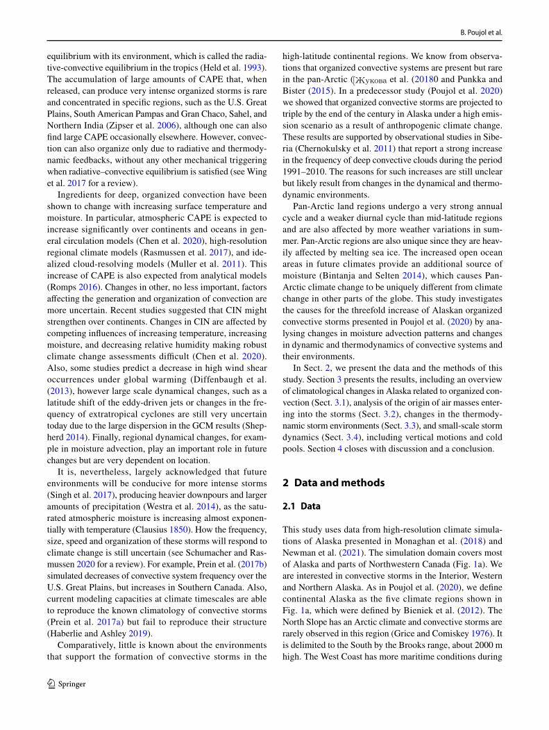
Figure 2a, shows that summer-mean near surface relative humidity is already almost at saturation over the oceans in the current climate. It is, therefore, reasonable to hypoth-esize that relative humidity is maintained at a high value by local evaporation over the ocean, and therefore that rela-tive humidity does not vary a lot over the oceans. Using the climatological values of temperature in Interior Alaska and the Bering Sea (respectively 15 °C and 7 °C), relative humidity in the same regions (respectively 0.6 and 1) and temperature changes in July (respectively +4 °C and +4.5 °C), this simple model predicts a 5% increase in continental relative humidity in Alaska. This theoretical value is close to what the model simulates (Fig. 2b), and therefore the sea–ice albedo feedback and the subsequent land–sea contrast under warming appear to be responsible for a moistening of Alaska in summer. This is unique in high-latitude land regions since most continents experience drying with climate change, mainly due to the land–sea warming contrast (Joshi et al. 2008 and Byrne and O’Gorman 2018). This moistening is constrained to the low atmospheric levels and very small changes are observed above 800 hPa (about 1500 m above

(4)cp�Tland + Lv�qland = cp�Tocean + Lv�qocean.

sea level). Moreover, Fig. 2d shows that over land, relative humidity changes are statistically significant only below 900 hPa. It is interesting to notice that whereas the Arctic Ocean experiences little relative humidity changes at the surface at the end of the summer, like the other ocean basins, it expe-riences strong moistening in the lower layers in May–June when most of it is still frozen both in the historical and PGW simulations (Fig. 2b). It therefore behaves like a continent in the early summer.

Finally, mean wind at 850 hPa is shown on Fig. 2a, b. In the Interior regions, the mean circulation is weak which sug-gests that convective storms generally occur in a barometric swamp. This is also supported by the low average movement speeds of convective storms (Poujol et al. 2020). However the West coast and the North Slope are dominated by South-erly winds. These winds appear to become weaker in a future climate. This result must be taken with caution, as the PGW scenario only captures monthly changes of the synoptic cir-culation. Alaska moisture transport is dominated by meridi-onal circulations that shift between Northerlies and South-erlies and moisture is mostly transported by transient eddies (Naakka et al. 2019). Furthermore, Tachibana et al. (2019) showed that strong sea ice loss in the Bering and Chukchi seas can generate a persistent positive geopotential height anomaly in these regions, and affect large-scale circulation over North America. In particular, this last effect could be an explanation for the observed weakening of Southerlies. Note that no important changes in low-level vertical wind shear occur between the two simulations, probably owing to the PGW methodology. As shown on Fig. S1, climatologi-cal wind shear is weak in the region of interest (difference of about 5 m/s over 100 hPa for shallow wind shear and 9 m/s over /450 hPa for deep layer shear), two to three times smaller than typical values in the U.S. Great Plains for exam-ple. Moreover, changes in wind shear are non significant between the historical and the PGW simulations. Also, no statistically significant changes in soil moisture content or evaporation occur in the simulations, except in the North Slope where the soil contains more water in a future climate, possibly due to permafrost thaw (not shown).

Warming and moistening are the dominant simulated changes in the region. The rest of this study investigates the effect of these changes on future organized convective storms focusing on the reasons for their threefold increase in frequency (Poujol et al. 2020).

3.2 Origin of the storm air masses

Backward tracking of the air masses entering into the storms has been performed in order to better understand the synop-tic-scale patterns associated with the convective storms and


1 3

the properties of the air masses feeding them. The tracking framework is described in the Sect. 2.

To provide an example, Fig. 3 shows the results of this air mass tracking for the convective storms occurring over the North Slope. Panel a shows the track frequency of the par-cels released from convective storms and tracked backwards. The frequency is largest in the North Slope itself; however some tracks cover a large part of the domain including the Gulf of Alaska, the Bering Sea, and the Arctic Ocean. The mean parcel relative humidity, shown in panel b, is close to the surface climatological relative humidity over land. However, over the ocean, parcels have a much lower relative humidity than the surface climatology, which is likely due

to the fact that some parcels are not at the surface but above, where mean relative humidity is lower (Fig. 2c).

Consistently, the moisture uptake (shown in panel c) is very local, which suggests that the storms occur under weak dynam-ical forcing, as already suggested by the climatological wind speed on Fig. 2a. This also shows that the recycling ratio is high for these storms. However, this should be taken with cau-tion, as the study domain is small, and evaporation over marine areas is prohibited by a low-level troposphere that is almost saturated (Fig. 2). Therefore, even if the moisture uptake is local, air parcels still convey properties from oceanic basins that they originate from before moving onto the continent.

Under future climate conditions (panels d–f), much more air feeding the storms comes from the Arctic Ocean,

Fig. 2 a Mean relative humidity in the summer (May–August) in the control simulation. Arrows indicate mean wind at 850 hPa in the control simulation. b Mean relative humidity change (shadings) and mean change of 850 hPa wind. Dotted areas indicate a significant relative humidity change at a 95% confidence level according to a two-tailed Student’s t test Student (1908). Wind changes are not sta-tistically significant. c Mean relative humidity profile in the five sub-

regions of interest under current climate conditions averaged during the warm season (May–August) except for the Arctic Ocean as indi-cated in the legend. d Mean change in relative humidity as a function of height in the subregions of interest. Dots on the right of the panel indicate a statistically significant change with 95% confidence accord-ing to Student’s t test. In c, d, triangles on the x-axis show relative humidity and its change at 2 m

B. Poujol et al.

1 3

potentially owing to the strong warming of this area due to the retreat of sea ice. The mean relative humidity of the parcels is increased over the whole domain, but this increase is much more pronounced over the Arctic Ocean. This is also visible in the moisture uptake from the Arc-tic Ocean, that increases by 50% (when normalized by the increase in the number of storms). All these changes suggest that melting sea ice and increasing sea surface temperature in this region provide an additional source of moisture for future convective storms.

The results in the other subregions are similar. Supple-mentary Fig. S2 depicts the results for storms over the Cen-tral Interior, which are representative of the other subregions as well. The moisture uptake is mainly local and parcels come from the three marine basins. In the future, no strong changes are observed except for an increase of the relative humidity of the parcels over land and over ocean.

For easier comparison and understanding of the origin of air masses, parcel frequency has been aggregated by ocean basin in Fig. 4a, c. Also, Fig. 4b, d shows the repartition of the origin of parcels (i.e. the location of the parcel at the end of the backward tracking within the study domain). Although parcel frequency is highest over land, most par-cels originate from marine basins. Air coming from the Gulf of Alaska contributes most to storms (about 50% of the air mass origin), which is not surprising given that it is the warmest ocean basin. However, more parcels originate from the Arctic Ocean and the Bering Sea at the end of summer, when these basins are ice-free. The two different approaches (parcel frequency or parcel origin) give similar results on the ranking of marine basins in moisture origin for all subregions, and how they change in a future climate.

In a future climate, the proportion of air masses com-ing from the Bering Sea and the Arctic Ocean increases

a c e

b d f

Fig. 3 Results of the backward tracking analysis for the parcels released in the North Slope’s convective storms. a Normalized parcel track density on a coarse grid of the model domain. c Mean relative

humidity of the parcels. e Normalized moisture uptake from the par-cels. b, d, f Same as a, c, e, but in the PGW simulation


1 3

for all the subregions except the West Coast, especially in July–August. Generally, this increase occurs at the expense of the proportion of air masses coming from the Gulf of Alaska. This means that in a future climate the proportion of storms that are fed by Arctic air masses is larger.

Changes in the frequency of origin of air parcels can also be interpreted using the Bayesian probability theory. For a given subregion, let S be the event “A storm occurs in the subregion” and O a random variable representing the ori-gin of the air mass. According to the Bayes’ formula Bayes (1763):

where x is an arbitrary ocean basin. The left-hand side cor-responds to the probability that an air mass feeding a storm comes from a given ocean basin, which is shown in Fig. 4. It is equal to the probability that a storm occurs when the

(5)ℙ(O = x|S) = ℙ(S|O = x)

ℙ(S)× ℙ(O = x),

low-level air mass comes from this basin normalized by the number of storms (left-hand factor of the right-hand side), multiplied by the probability that the air mass comes from this basin (right-hand factor). Since there are no changes in the dynamical day-to-day variability in the simulations, the last factor ℙ(O = x) remains almost constant between the simulations. (This assumption could be checked by investigating the origin of the air masses on days when no convection occurs, however this was not done in this study due to computational constraints.) Therefore, changes in the frequencies shown in Fig. 4 directly reflect changes in the normalized probability that an air mass coming from a given oceanic basin is associated with the triggering of a convec-tive storm. Therefore, it stems from these probabilistic con-siderations that air masses coming from the Bering Sea and the Arctic Ocean are more likely to be associated with con-vective storm initiation in almost all subregions in a future climate. (Note that this conclusion could not be drawn if the

a b

c d

Fig. 4 Origin of the air masses feeding the storms. a For each subre-gion, and for the historical and PGW simulations, bars represent the parcel density along their whole trajectory over land and the three ocean basins in May–June. b Bars represent the distribution of the

origin of air parcels, which is defined at the location of the parcel at the end of the backward trajectory. c, d As a, b but for July and August

B. Poujol et al.

1 3

simulations included changes in the dynamics). This can be due to the strong sea ice retreat, providing an additional source of moisture, as well as the amplified warming and moistening of the atmosphere subsequent to sea ice loss in these regions. The fact that this increased contribution from Arctic marine basins is largest at the end of summer, when sea ice loss is the strongest, further supports this hypothesis.

3.3 Changes in the thermodynamic convective environments

3.3.1 CAPE and CIN climatology

Figure 5 depicts the joint distribution of horizontally aver-aged most unstable CAPE and CIN in the afternoon (16:00 local time) over two representative subregions. Environ-ments favorable to deep and organized convection are rare

Fig. 5 Joint distribution of most unstable CAPE and CIN averaged over the West Coast (a, b) and Central Interior (c, d) at 16:00 p.m. local time (AKDT), from May to August. Marginal distributions are shown in gray. a, c Control simulation. b, d PGW simulation. Note

the logarithmic scale of the colorbar and the marginal distributions. A Gaussian smoothing with a radius of 1 is applied to the distributions. Stippling indicates a 95% confidence significant change according to a monthly block bootstrap test


1 3

in the current climate simulation. Subregion-averaged CAPE is usually below 100 J/kg, which is usually insufficient for organized convective storms to develop (Kirkpatrick et al. 2011). Indeed, as it will be shown later, the storms that we track in this study tend to develop in environments with CAPE values ranging from 200 to 600 J/kg and CIN values below 15 J/kg. Such CAPE values are in the tail of the cur-rent climate distribution causing these storms to be rare: in the current climate simulation, they have a recurrence period of once per year South of the Yukon river and longer in the Northern part of Alaska (Poujol et al. 2020). The tail of the distribution extends towards much higher values of CAPE in the PGW simulation, however CIN changes differ across subregions.

In the West Coast, the tail is extended towards high-CAPE and high-CIN environments, similarly to what has been simulated in the U.S. Great Plains (Rasmussen et al. 2017). This will likely favor more intense and organized systems, however more energy will be necessary to trig-ger deep convection. In contrast, in the Central Interior, the distribution is extending towards high-CAPE and low-CIN environments. These environments are extremely favorable for organized, deep convection, as an increased amount of energy is available for deep convection and can be easily released.

The Northeast and Southeast Interior subregions show a behaviour very similar to the Central Interior whereas the North Slope experiences changes in-between the West Coast and the interior with increases in high-CAPE and moderate-CIN environments. In any case, the increase is much larger in the tail of the distribution. For example, environments with CAPE > 300 J/kg and CIN > − 5 J/kg in the Central Interior region are five folding in the future simulations.

3.3.2 Storm inflow soundings and mathematical model

In order to explain these large changes in thermodynamic environments, a simple model is used that simulates the effect of changes in surface temperature and relative humid-ity in some key features of the environment. This mathe-matical model is a tool in order to make simple sensitivity experiments and disentangle the roles of different physi-cal processes in the changing characteristics of convective storms. For the sake of simplicity, this is based on an analyti-cal model developed by Romps (2016).

The main hypothesis is that the environment profile obeys a Radiative–Convective equilibrium (RCE), i.e. the profile of temperature is a balance between the radia-tive transfers of energy in the atmosphere, and the mix-ing and latent heating provided by convection. Grice and Comiskey (1976) noticed that deep convection occurs

nearly every day in Alaska in June and July and that most Alaskan thunderstorms are of the air-mass type (i.e., they are triggered by solar forcing and are not associated with a large-scale forcing). However, this is not sufficient to assume radiative-convective equilibrium because dynami-cal disturbances and large scale forcing can occur over time scales shorter than weeks. Given this, the mathemati-cal model is used only for a qualitative comparison and for a physical interpretation of the results. It is not intended to (and does not) reproduce quantitatively the results of the simulation, but it allows to qualitatively assess the depend-ency of key environmental variables, such as CAPE and CIN, on surface temperature, specific humidity, and rela-tive humidity, and the model helps to feed the scientific discussion of the results.

All variables are defined in the appendix. Notably q∗ refers to saturated mixing ratio, Ts refers to surface tem-perature, Tc refers to a typical scaling temperature for the Clausius–Clapeyron law (here fixed to 23 K) and T0 is some reference temperature. As shown by Romps (2016), RCE can be expressed by the conservation of environmen-tal moist static energy defined as:

where a is defined as:

with PE the precipitation efficiency and � the entrain-ment/detrainment rate. a is therefore a parameter depend-ing on cloud physics and regulating the environment lapse rate between a dry adiabatic ( a = ∞ ) and moist adiabatic ( a = 0 ). Since the model is used here for a qualitative com-parison only, no particular value of a is determined. How-ever, for graphical representations, the value a = 1 is arbi-trarily chosen (it produces profiles that are reasonably close to the model data). The tropopause temperature is assumed constant at TFAT = 238 K Hartmann and Larson (2002). Dif-ferently from Romps (2016), where the parcel is assumed to be saturated from the surface, we add a new variable which is relative humidity in the boundary layer. We therefore add the possibility to have a lifted condensation level, and CIN. Therefore, the model only depends on two parameters that are surface temperature and surface relative humidity. Although it is extremely simple, it accounts for the changes in the atmospheric lapse rate that are visible in Fig. 1b. This enables the calculation of several thermodynamic variables by lifting the surface parcel into its environment. Analytical expressions can be obtained through some relatively weak assumptions:

(6)he = cpT + gz +Lvq

∗

1 + a,

(7)a =PE �

−�z ln(q∗),

B. Poujol et al.

1 3

• Moist static energy of the parcel is conserved during its ascent (undilute plume).

• Saturated moisture depends exponentially on tempera-ture q∗(T) = q∗

sexp((T − Ts)∕Tc).

• Relative moisture variations are large compared to rela-tive temperature variations.

• Virtual effects are neglected.• Atmospheric heat capacity, gravity acceleration and

latent heat of vaporization are taken constant.• Specific humidity and mixing ratio are taken equal.

This provides the following expression for CAPE:

(Refer to Romps (2016), Sect. 4 for the detailed calcula-tion.) The expression of the LFC temperature TLFC can be found in the appendix (Eq. 28) and depends both on surface temperature and surface relative humidity. However, mois-ture increases much faster than temperature, at the Clau-sius–Clapeyron rate (hereafter CC scaling) (Clausius 1850). Therefore, CAPE increases should experience a CC scaling

(8)CAPE =a

1 + aLv

q∗(TLFC)

T0(TLFC − TFAT − Tc).

with the temperature increases of the level of free convec-tion. CAPE also increases with surface relative humidity through the dependence of TLFC on RH; the moister RH, the lower and thus the warmer the LFC. The same model gives the following formula for CIN:

where f is always negative, and |f| decreases with relative humidity and with a. The analytical formula for function f can be found in the appendix (Eq. 31). This suggests that under constant relative humidity, CIN should also scale with surface atmospheric moisture and therefore experience CC scaling. However, one should bear in mind that f has a loga-rithmic and therefore somewhat sensitive dependence on RH.

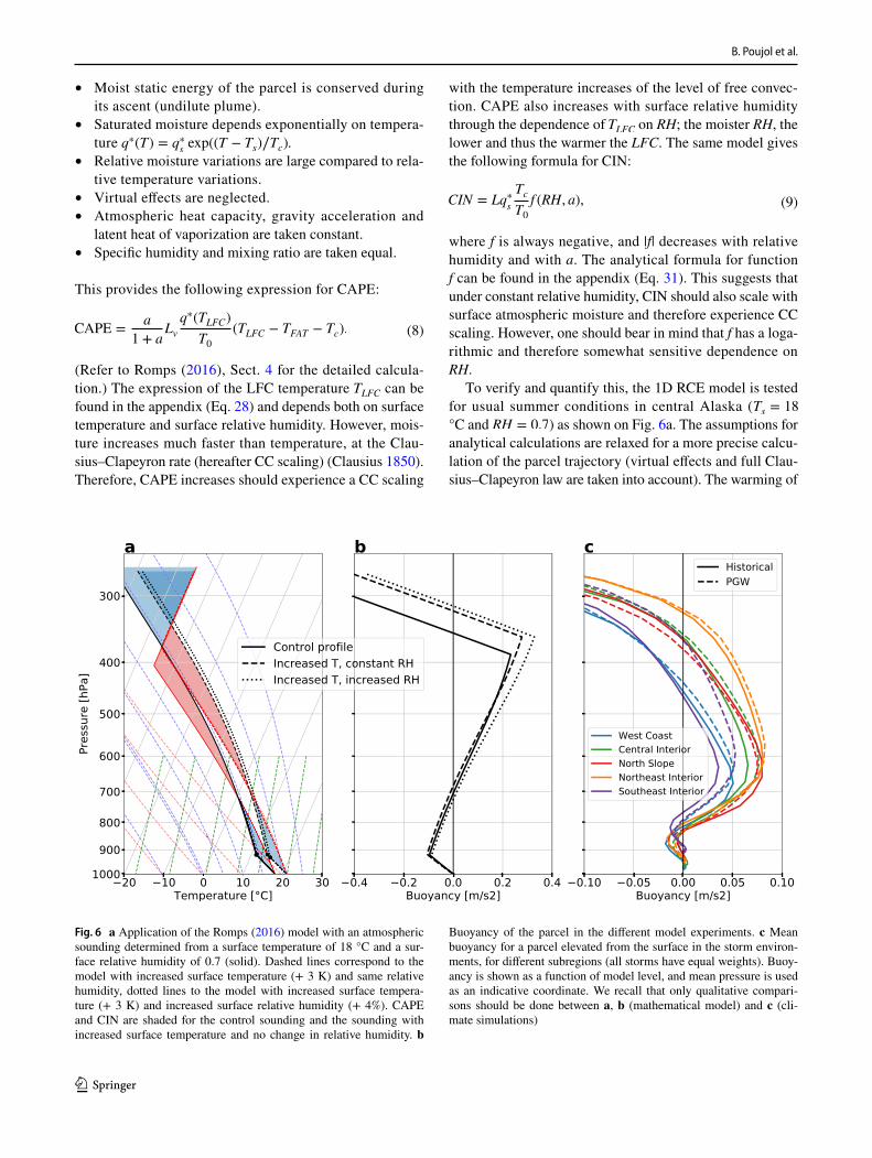
To verify and quantify this, the 1D RCE model is tested for usual summer conditions in central Alaska ( Ts = 18 °C and RH = 0.7 ) as shown on Fig. 6a. The assumptions for analytical calculations are relaxed for a more precise calcu-lation of the parcel trajectory (virtual effects and full Clau-sius–Clapeyron law are taken into account). The warming of

(9)CIN = Lq∗s

Tc

T0f (RH, a),

Fig. 6 a Application of the Romps (2016) model with an atmospheric sounding determined from a surface temperature of 18 °C and a sur-face relative humidity of 0.7 (solid). Dashed lines correspond to the model with increased surface temperature (+ 3 K) and same relative humidity, dotted lines to the model with increased surface tempera-ture (+ 3 K) and increased surface relative humidity (+ 4%). CAPE and CIN are shaded for the control sounding and the sounding with increased surface temperature and no change in relative humidity. b

Buoyancy of the parcel in the different model experiments. c Mean buoyancy for a parcel elevated from the surface in the storm environ-ments, for different subregions (all storms have equal weights). Buoy-ancy is shown as a function of model level, and mean pressure is used as an indicative coordinate. We recall that only qualitative compari-sons should be done between a, b (mathematical model) and c (cli-mate simulations)


1 3

3 K indeed causes an increase in CAPE and CIN (i.e. more negative CIN), similarly to the results of Rasmussen et al. (2017). These increases are close to the Clausius-Clapeyron scaling (+ 30% for CAPE and 23% for CIN), as expected from the analytical equations. However, increasing relative humidity by 4% (dotted line) increases CAPE by 29% and decreases CIN by 28% compared to the control sounding. This leads to an eventual increase in CAPE by 68% and a decrease in CIN by 12%. In the end, warming and moisten-ing both impact CAPE, while moistening dominates the CIN response.

The buoyancy profile of these changes is shown in Fig. 6b. It appears that the increase in CAPE generated by warming alone (and subsequent lapse rate adjustment) results in an increase in buoyancy at high levels only (com-pare solid and dashed lines), mainly owing to the increase in tropopause height. This is consistent with the results of Seeley and Romps (2015), Singh and O’Gorman (2013) and Parker (2002) who noticed that CAPE is essentially modu-lated by the depth of the layer of positive buoyancy. One can even see that buoyancy slightly decreases in the lower troposphere compared to the control parcel. Conversely, moistening produces an increase of buoyancy that is almost constant through the tropospheric column (compare dashed and dotted lines). Therefore, these characteristic and dif-ferent signatures support the hypothesis that moistening strongly enhances CAPE increase in the simulations.

Figure 6c shows that buoyancy increases through the whole troposphere in the Interior regions in the WRF simu-lations, whereas in the West Coast it increases mainly in the upper troposphere. A qualitative analogy between this result and results from the mathematical model presented in the last paragraph suggests that the influence of surface moistening on atmospheric instability mainly arises in the interior regions and is consistent with the CAPE/CIN dis-tribution extending toward strong CIN environments in the West Coast (the temperature effect dominates) and weak CIN environments in the Interior (the surface moistening effect dominates) (Fig. 5). It is also consistent with the larger low-level moistening of the Interior region compared to the West Coast (Fig. 2b). In the North Slope, a decrease in buoy-ancy is found, but the small number of storms in the control simulation (58) likely makes the historical composite buoy-ancy profile not very robust.

The fact that buoyancy increases across the whole tropo-sphere due to surface moistening is of particular interest. Indeed, this implies that storms are affected by the changing thermodynamic environment even during their early devel-opment stages since buoyancy already increases at low lev-els. This could support the onset of convective organization and convective updrafts to be more vigorous. Conversely, in the case of a warming without increases in relative humidity, deep convection will only be affected by buoyancy increases

once it has reached the upper troposphere, which is likely a storm that is close to or already mature. The impact on con-vective organization would therefore be much smaller. The impact of the vertical distribution of buoyancy can be con-siderable, as Kirkpatrick et al. (2011) found that in storms of moderate CAPE (like most of the storms considered in this study), the maximum updraft speed can vary by a factor of 6 depending on the vertical distribution of buoyancy. In their set of simulations, lowering the altitude of maximum buoyancy could make the difference between a short-lived and a persistent convective storm, without changing CAPE. This could be one of the reasons why we find a threefolding of organized convective storm frequency in Alaska under future climate conditions.

Several variables from the analytical models are shown in Fig. 7, together with the joint and marginal distributions of these variables for storm environments in the historical and PGW simulations. Since no quantitative agreement is expected between the analytical curves and the climate simu-lations, it is not surprising to see that the model results do not follow the analytical curves very well. Here, the analyti-cal model is provided for qualitative comparison only.

Panel a shows the distribution of temperature and CAPE. The storms occur under a broad range of surface temperature and CAPE values. The largest values of CAPE roughly fol-low the changes in CAPE from the analytical model. As a result, in the PGW simulation, where the temperature range extends to larger values, high CAPE values increase follow-ing a Clausius–Clapeyron scaling.

Changes in CIN (panel b) also show that extreme CIN values follow the temperature relationship. Mean CIN binned by temperature is similar in the two climates, how-ever more storms have extremely low values of CIN in the PGW simulation, as it is visible in the marginal distribution. Given the shape of the theoretical curves, it is likely attrib-utable to the increase in surface relative humidity. This is compensated in the mean by the extreme CIN values that are larger in the PGW simulation. To summarize, the tail of the CIN distribution extends towards more extreme values (due to warming) but the distribution has also larger values very close to zero (due to moistening), whereas moderate values of CIN occur less frequently under future climate conditions.

Two other variables of interest are represented. The freez-ing level height is shown on panel c. The analytical model expression for the freezing level height is:

The first term would be the freezing level for a parcel that never crosses the LCL and increases linearly with surface temperature. The second term is a moisture correction that increases strongly with temperature, both through the

(10)zf =cp

g(Ts − Tf ) +

Lq∗s

g

(RH − exp

(Tf − Ts

Tc

)).

B. Poujol et al.

1 3

saturated surface moisture on the left, and the factor depend-ent on surface temperature on the right. It increases line-arly with surface relative humidity. Freezing level height increases significantly between the historical and PGW simulations, from 2400 to 2900 m on average (panel c). The PGW mean is so high that it is almost located in the tail of the current climate distribution. On top of that, the LCL height decreases from about 700–600 m (not shown) due to the relative humidity increase. This represents a 35% increase in warm-cloud layer depth (from 1700 to 2300 m) that could substantially affect storm dynamics and precipita-tion efficiency (Prein and Heymsfield 2020). It has indeed been found that deep warm-cloud layers can favour more intense precipitation through collision and coalescence (Doswell 2001). It appears on the figure that average freez-ing level height increases with surface warming. However, for the same surface temperature, storms in the PGW simula-tion still have a higher freezing level than storms in the his-torical simulation. According to the theoretical model, this can be explained by the surface moistening, that is respon-sible for about 250 m increase in the freezing level height, i.e. half of the total change. The same conclusions can be drawn from panel d: for the same temperature, the level of free convection is lower for storms in the PGW simulation than in the historical simulation. This also corresponds to an increase in surface relative humidity. The marginal distribu-tion on the right points out that future storm environments have lower LFCs than current climate storms, which means that the moistening effect dominates the temperature effect for this variable. Note that slopes of the freezing level as a function of temperature are less steep for the dynamically simulated storms than predicted by the RCE model, while the opposite occurs for the LFC. This is likely due to the fact that warmer storm environments also tend to be drier in this set of simulations (not shown).

In summary, environmental changes between the two simulations become very conducive for deep convection and convective organization. Indeed, for some variables, such as CAPE or the freezing level height, the effects of warming and moistening add up and provide very strong changes. Other variables, like CIN and the LFC, should evolve with temperature in a way that decreases the likelihood of con-vective storms to occur. However, for these variables, the surface moistening has an opposite effect that eventually dominates the climate change signal.

3.4 Changing storm dynamics

3.4.1 Storm structure changes

Figure 8a, b shows the composite cross-section of histori-cal storms during their first 6 h. The storms are rotated for compositing so that the direction of the maximum surface

equivalent potential temperature gradient (thereafter �e ) is on the right. The inflow area of the storm is, therefore, on the right. The inflow air is conditionally unstable to moist convection given the negative vertical �e gradient, whereas the outflow region (on the left) is stable. The structure of the storms is very similar to the archetypal structure of mid-latitude and tropical mesoscale convective systems (Houze 2004). A thick layer of high-�e air feeds the storm and is advected towards the upper troposphere, whereas rear-inflow is confined in a thin layer close to the surface. A gust front resulting from the downdrafts is visible 60 km ahead from the storm precipitation maximum. This front materializes the location of surface mechanical forcing that enables the storm to trigger new cells, or maintain the existing cell, and therefore persist for several hours. Indeed, high-�e air moves upward along this front. Equivalent potential temperature increases while the air moves upward, probably due to the entrainment of environmental air into the system. The storms produce condensate on very large spatial scales, and in par-ticular have a large anvil in the upper troposphere, which is characteristic of organized convective systems. These storms exhibit strong low-level vorticity and core vortical towers extending to the middle of the troposphere. Composites on Fig. S3 show that they have a rotating circulation that con-verges ahead of the storm close to the surface, and in the core of the storm at 850 hPa and above.

Future storms are substantially different from current storms in several ways (panels a, b and d, e). First of all, the equivalent potential temperature increases by almost 10 K at low levels in the storms. A rapid calculation using the defini-tion of �e shows that this increase is mainly due to changes in saturated moisture (60%) with minor contributions from temperature increase (30%) and increase in relative humid-ity (10%). Changes in the condensate are also visible, in particular a strong increase of condensate loading in the core of the storm, and a decrease of ice content at 400–500 hPa likely attributable to the increase in freezing level height. Also, noticeable changes affect vertical movements in the storms. Future storms have stronger updrafts in the low levels (600–800 hPa) despite their increased condensate loading. This confirms the hypothesis formulated using the buoyancy profiles while discussing Fig. 6 (i.e., buoyancy increases and updrafts become stronger through the whole tropospheric column). Updrafts are also more intense at the top of the troposphere (300–400 hPa) probably owing to the temperature increase effect on buoyancy related to the deepening of the troposphere. This results in deeper convec-tion and higher cloud tops under future climate conditions. Also, a weakening of downdrafts occurs that brings the gust front closer to the storm (panels b, e). This might weaken the rear-inflow and the advection of low-�e air into the storm boundary layer, and generate new convective cells closer to the storm, which could favor storm organization.


1 3

Figure 8g depicts the composited mass flux contribu-tion from different vertical wind speeds in the storms at 850 hPa (updrafts and downdrafts are composited at the same time, and the mass flux is integrated over the area that corresponds to the convective storms as identified by the tracking algorithm). For small speeds, below 0.5 m/s, upward and downward mass fluxes are almost identical and probably correspond to atmospheric turbulence that is not significantly affected by water phase change processes. Above this threshold, the mass flux contribution from updrafts is larger than the one from downdrafts. In a future climate, storms exhibit much larger upward mass fluxes. The updraft speed that has the peak contribution is slightly higher in the future climate, despite the larger condensate loading, which might result from larger CAPE. However, intense downdrafts ( w < −1m s−1) show a much reduced mass flux contribution in the future. Figure S4 also shows the probability of presence of updrafts and downdrafts in the storms and how it changes in a future climate. One can see that strong updrafts ( w > 1 m/s) are more frequent in the core of future storms, whereas strong downdrafts become less frequent in the storms, across the whole tropospheric column. One can also notice that updrafts become less frequent in the inflow region of the storms and narrower in the core of the storm, but we leave open the interpretation of this result. We suggest that this weaken-ing of downdrafts is due to a decrease in the evaporation of precipitation related to an increase in low tropospheric relative humidity. Panel h indeed shows that storms are already very moist at the surface in a current climate, but future storms have even higher relative humidity. In par-ticular, storms that are saturated at the surface are 60% more frequent under a future climate, which could explain the weaker downdrafts. Panels b and e also clearly show an increase of low-level relative humidity within the storms.

Such decrease in downdraft frequency with increasing relative humidity has been noticed during observational campaigns, for example in the Amazon region where radar wind profilers revealed that squall lines have stronger and deeper downdrafts during the dry season than during the wet season (Wang et al. 2019). This study also found stronger and deeper downdrafts in the U.S. Great Plains where the relative humidity is lower than in the Amazon. This is dif-ferent to other idealized studies (e.g. Schumacher and Peters 2017), which found that increasing relative humidity causes an intensification of precipitation, and therefore stronger evaporation. They found that this last effect balances and even overcomes the direct weakening effect of relative humidity on evaporation.

It is possible that the weaker downdrafts in the future favor the organization of convection. Downdrafts tend to favor the dissipation of convective cells and lead to the for-mation of cold pools, that can only trigger new convective

cells at their edges, while they prevent convection in the immediate vicinity of the downdraft that created them (Zipser 1969). It has been found in numerical simulations that removing precipitation evaporation in the lower tropo-sphere can lead to the organization of convection, although these experiments were made under idealized tropical mari-time conditions (Jeevanjee and Romps (2013) and Muller and Bony (2015)). The mechanisms for this organization are still unclear, but moisture feedbacks are likely responsible.

Although these mechanisms were observed/simulated in tropical environments, we do not see any particular reason why they would not be relevant for higher latitudes.

3.4.2 Cold pool dynamics

Another relevant parameter to convective organization is the role of cold pools in the mechanical and thermodynamic triggering of deep convection (Schlemmer and Hohenegger 2014). Their role in convective organization is still not well understood. While some studies found a favoured convec-tive organization when cold pools are artificially removed from idealized simulations (Jeevanjee and Romps (2013) and Muller and Bony (2015)), other studies found that cold pools favor convective organization (Haerter (2019) and Hirt et al. (2020)) and the formation of tropical cyclones (Davis 2015). Nevertheless, most of these studies focus on mid-latitude or tropical environments and little is known about continental high latitude regions. The main takeaway is that cold pools can decrease low-level buoyancy under a storm and lead to its dissipation, but they can also trigger new con-vection through the mechanical circulation induced by their movement and collisions (Henneberg et al. 2020).

Similarly to precipitation we track cold pools (contiguous areas of negative buoyancy) in the simulations. However, the results presented in this section must be taken with caution. Although cold pools can be represented at a grid spacing of 4 km, this representation might be too coarse to capture climate change impacts on cold pool properties (Prein et al. 2020). Moreover, it is obvious that this resolution is not suf-ficient to capture the small-scale mechanisms that occur at the edge of the cold pools, such as accumulation of moist, high-�e air and the presence of a small-scale gust front. The detailed methodology for cold pool tracking is presented in the Sect. 3.

Figure 9a shows the June–July diurnal cycle of cold pools. The frequency of cold pools peaks in the middle of the afternoon. This is concomitant with the observed diurnal cycle of lightning in Alaska (Poujol et al. 2020) indicating that cold pools are strongly associated with deep convec-tion. The peak of cold pool frequency, however, occurs well before the peak of organized convective storms (Poujol et al. 2020). Moreover, the number of cold pools does not follow the tripling of convective storms and only increases from

B. Poujol et al.

1 3

3275 in the control simulation to 3663 in the PGW simula-tion. It is therefore likely that most cold pools are produced by single cells, that are much more numerous than organ-ized convective storms and cause the early peak in the day, concomitant with the lightning peak.

Interactions between cold pools and convective storms were investigated. Each time a cold pool and a convec-tive storm were partially superposed, an interaction was counted. About 10% of storms experience interaction with cold pools in the historical simulation (12% in the PGW simulation). But given that the number of storms triples, this also means a tripling of the interactions between storms and cold pools. However, this proportion is likely underestimated as some cold pools are missed because their negative buoyancy is too weak. They can also inter-act with the storm but are not completely superposed with it, or they dissipate before the storm produces any precipitation.

Cold pool size and storm size are composited around their interaction time (shown as 0 h) in Fig. 9b. Interac-tions tend to occur during the phase when the cold pools are the largest, and when the convective storms are in their early development (i.e., convective storms are on average 4 times larger 2 h after the interaction compared to 1 h before). This implies either that cold pools are triggering convection, or that they are produced in the early stages of the storms and dissipate shortly afterwards. Also, we count interactions between cold pools and storms while artificially lagging them by a certain amount of time. For example, a lag time of 2 h means that a cold pool was present 2 h before precipitation was detected at the same location. It appears that at a given location, cold pools frequently precede organized convective storms by 0–2 h (Fig. 9c). Precipitation preceding cold pools is much rarer. It therefore suggests that cold pools play a role in the setup of organized convective storms, although no causality link can be deduced from this analysis.

We would like to underline that the signals visible in Fig. 9b cannot be solely explained by the diurnal cycles of cold pools and organized storms. Indeed, whereas the diur-nal cycle amplitude of organized convective storms has a factor two (two times more storms in the evening compared to the late morning), panel b shows that organized storms tend to be four times larger after the interaction with a cold pool compared to before.

Figure 9d–f shows a representative event where two cold pools, associated with two moderately active precipitation systems, merge and eventually generate an intense precipita-tion event after merging. This precipitation patch then grows to a larger storm identified as an organized convective storm by the tracking algorithm (not shown). This example shows that cold pools can play a role in triggering organized con-vective storms.

4 Discussion and conclusion

Figure 10 summarizes this work and previous work on the physical mechanisms responsible for changes in the frequency of convective storms in Alaska. Anthropo-genic warming causes a moistening of the region, due to the increase of saturated humidity governed by the Clau-sius–Clapeyron law (Clausius 1850). This wetting produces an intensification of extreme rainfall in organized convec-tive storms as it was shown in Poujol et al. (2020). Another reason for this precipitation increase might be the increase in the freezing level that could affect precipitation efficiency, however this effect should be small compared to the previ-ous one as storm precipitation intensification was found to scale with atmospheric moisture (Poujol et al. 2020). As highlighted in the schematic, sea ice loss and the subsequent land–sea warming contrast are responsible for an increased relative humidity in Alaska. (Note that this is only valid in summer, as in winter insolation is weak and sea ice loss can lead to cooling through radiative feedbacks.) This favors the onset of deep, organized convection through many physical mechanisms and appears to be key to explain the tripling in the number of storms. Sea ice loss provides an additional source of moisture in a future climate, and air masses com-ing from the Arctic Ocean or the Bering Sea will be more likely to trigger convective storms in a future climate, espe-cially in the North Slope.

This study also suggests, through the analogy between an analytic thermodynamic model and the climate simula-tion results, that the warming and raising relative humid-ity increase CAPE, decrease CIN, and lower the LFC. Our results suggest a strong relationship between the increase in storm frequency and these thermodynamic changes. The effects are the strongest for CAPE and for the LFC, where the distributions clearly differ between the control and the future simulation (Fig. 7). However, we do not establish a causal relationship. Previous work focusing on mid-latitude storms demonstrated that large CAPE (more than 450 J/kg) is necessary to enable the development of organized, self-sustaining convective storms (Kirkpatrick et al. 2011) and that CAPE is strongly related to the number of convective cells in the storms. Therefore, high CAPE conditions are strongly favorable for multicell storms to occur. The impact of decreasing CIN is less obvious, since it has been shown that low CIN environments favor convection only under very weak large-scale forcing (Zhang 2002). Zhang (2002) found that as long as some forcing is present, deep convection can occur even in an environment with very high CIN values.

Changes in the storm dynamics also affect future organ-ized convective storms in Alaska. We find a strong, statisti-cally significant weakening of downdrafts in future convec-tive storms despite the intensification of precipitation. This is likely due to the increase in relative humidity within the


1 3

storms, with the future storms being 60% more likely to reach saturation at the surface, which reduces the evapora-tion of rain and therefore weakens downdrafts. This weaken-ing of downdrafts could help organizing and sustaining long-lived convection through moisture feedbacks. This appears to be one of the dominant causes for the large increase in the frequency of organized convective systems. More uncertain are the impacts of cold pools on convective organization. In the simulations, cold pools were found to peak in the early afternoon, whereas organized convective storms peak in the evening. Cold pools are therefore likely produced by monocellular, disorganized convection. They can propagate and favor an evening triggering of convection producing a second wave of organized, intense precipitation. This phe-nomenon has been observed in idealized large-eddy simula-tions (Lochbihler et al. 2019) and Haerter and Schlemmer

(2018) noted that in this second phase, precipitation clusters have a larger size than in the first phase. A potential positive feedback is shown in the schematic: more storms lead to more cold pools, and therefore more mechanical triggering. The number and intensity of cold pools does not change a lot in the simulations, probably owing to the weakening of downdrafts that counteracts the feedback. However, the lowering of the LFC suggests that dynamical triggering of convection by cold pools might become more frequent in a future climate. Nevertheless, all these possible feedbacks linked to cold pools remain hypothetic as no causality could be established by this study, due to the absence of sensitivity experiments or of a theoretical model.

The response of organized convection in Alaska is dif-ferent to responses that have been reported or modeled in other parts of the world. Observations reported strong

Fig. 7 Scatter plot of temperature and a CAPE, b CIN, c freezing level height, d LFC height. Each point represents the environment of one storm in the control (blue points) and PGW (red points) simula-tion. Solid blue and red lines respectively correspond to the centroids of blue and red points binned by temperature with bin edges defined as the 10th, 30th, 50th, 70th and 90th percentiles of the temperature distribution. Solid gray lines show the relationship expected from the

analytical RCE model, for different values of surface relative humid-ity (line color) as indicated in the legends. Marginal plots correspond to a normalized kernel density estimation of the blue and red points. Note that the legend is different on c compared to other panels. We recall that only qualitative comparisons should be done between lines (mathematical model) and dots (climate simulations)

B. Poujol et al.

1 3

increases of organized convective systems frequency in the tropical oceans (Tan et al. 2015) and in the Sahel (Taylor et al. 2017), but decreases in their frequency in Southeast Asia (Habib et al. 2019). Regional convection-permitting simulations predict an intensification of these convective systems due to the increased surface atmospheric moisture under a future climate, but a decrease in their frequency, for Africa (Kendon et al. 2019) and for the United States (Rasmussen et al. (2017) and Dai et al. (2017)). This set of Alaska simulations is different in the way that it pro-duces an increase in both the intensity and the frequency of organized convective storms. This study also simulated a decrease in CIN over Alaska due to sea ice loss and sub-sequent land cooling relative to the ocean. This is in sharp

contrast with the strengthening of CIN predicted over continents by GCMs and kilometer-scale models (Chen et al. (2020), Rasmussen et al. (2017) and Fitzpatrick et al. (2020)). Also, circulation changes have been shown to play an dominant role in the evolution of convective storms in several other regions (China (Zhang et al. 2017), Bangla-desh (Habib et al. 2019) and the Sahel (Fitzpatrick et al. (2020)) but were not investigated in this study. Indeed, only very large-scale and systematic dynamical changes are taken into account with the PGW approach. Therefore, caution should be taken as these results neglect changes that can be of significant magnitude, although uncertainty in the synoptic circulation changes is large. Similar simula-tions of the future climate in Alaska with full dynamical

Fig. 8 a Composite of equivalent potential temperature (shadings), wind speed (arrows) and cloud liquid and ice content (respectively solid and dashed contours) of the identified convective storms in the region of interest (May–August, all subregions mentioned in Fig.1a). Note that wind speed arrows have a vertical exaggeration factor of 10, whereas the vertical axis has a larger exaggeration factor (about 25). The center of the composites is the location of maximum precipita-tion and the storms are rotated for compositing so that the direction of the maximum surface potential temperature gradient is on the right. The vertical coordinate is model level, but mean pressure is indicated for easier reading. b Zoom of the grey box in a. Relative humidity is shown instead of equivalent potential temperature. c Composite of the mean vertical mass fluxes within the storms. d–f As a–c, but for

the storms in the PGW simulation. g Composite of the distribution of mass flux contribution from updrafts (red) and downdrafts (blue) in the storms at 850 hPa, for the historical (solid) and PGW (dashed) simulations. The following bin edges are used: w

n= 100.08n m s−1 ,

n ∈ [[−25 , 25]] . h Normalized distribution of surface relative humid-ity within the storms as identified by the algorithm, in the historical (solid) and PGW (dashed) simulations. In g, h shadings indicate the 95% confidence interval of a two-tailed bootstrap test by monthly blocks. a, b, d, e correspond to composites over the first 6 h of each storm, whereas c, f, g correspond to composites across the whole storm lifetime (i.e., storms lasting longer than 6 h can be counted sev-eral times)


1 3

forcing are planned and will give further insight into these processes.

The very strong increase in the number of convective storms in Alaska is quite unique, and it raises the question of the generalizability of this finding to other regions. This study identified the sea ice loss and the subsequent increase of rela-tive humidity over land as one of the dominant causes for the tripling in the number of storms. Therefore, it is possible that the same effect plays an important role in similar regions such as Scandinavia, Canada or Siberia. This would be con-sistent with the observed trend of an increasing convective activity over Siberia during the last decades (Chernokulsky et al. 2011). However convective storms in Alaska are also linked to the unique topography of the state, and therefore these postulates about other pan-Arctic regions should be investigated more deeply. Also, very few is known about the dynamical structure of high-latitude convective storms, for

example the role of the Coriolis force in their development and whether they have baroclinic characteristics or not. This lack of knowledge limits the interpretation of the results pre-sented in this study, especially concerning storm dynamics.

As can be seen on the schematic, all the arrows leading to the increase in the number of storms correspond to our hypotheses. Sensitivity experiments and targeted observa-tional studies would be necessary to better understand these processes. Idealized modeling studies should be conducted to better understand the impact of different thermodynamic environments on the frequency, size and intensity of con-vective storms, in particular in high-latitude environments. Also, dynamical mechanisms linked to cold pools and in particular the role of cold pools in convective organization deserve further investigation, as many studies show promis-ing results (e.g, Schlemmer and Hohenegger 2014, Haerter et al. 2020).

Fig. 9 a Diurnal cycle of simulated hourly cold pool frequency, observed lightning frequency Alaska Interagency Coordination Center—Alaska Fire Service (2020), and the frequency of organized convective storms in the historical simulation. b Composite of the area of the cold pools and of the storms relative to their first inter-action time. Each cold pool-and-storm interaction (i.e., coldpools area intersects with storm precipitation area) was considered with a weight of one, therefore storms interacting with several cold pools are counted twice and vice-versa. Shadings indicate the 90% confidence

interval from a two-tailed bootstrap test assuming that the interactions are independent. c Number of interactions between a storm and a cold pool as a function of the lag time taken between the two variables. A positive lag time indicates that cold pools exist before storm for-mation. d–f Example snapshots of precipitation (warm shadings) and negative buoyancy (transparent, cool shadings) in the control simu-lation on June 7th, 2004 in a subdomain, showing the interaction of two cold pools producing an updraft. Brown contours show smoothed topography every 250 m

B. Poujol et al.

1 3

Finally, there is a lack of literature about the environ-ments favorable to organized deep convection outside of the contiguous United States. In particular, very little is known about organized convective storms in high latitude regions, and even less about their triggering and develop-ment mechanisms and how they might change in a future climate. Our findings show that arctic environments have a unique response to climate change that is distinctly dif-ferent from tropical and mid-latitude regions. More work is necessary to better understand the underlying processes of these changes and their potential impacts on humans and ecosystems in high-latitudes.

Appendix : Details of the calculation of theoretical relationships

Framework

Usual notations are used. T is temperature, q is specific humidity, q∗(T) the saturated specific humidity, and qs = RHq∗(Ts) the surface specific humidity. g refers to Earth’s gravity acceleration, cp to the atmospheric heat capacity, Lv the latent heat of vaporization of water. Ra and Rv are the specific gas constants for dry air and water vapor. �d and �m respectively stand for the dry adiabatic and moist adiabatic lapse rates.

This calculation is based on the work of Romps (2016) who developed a conceptual model to calculate CAPE in tropical environments. Here, it is readapted to account for the possibility of the existence of CIN with an unsaturated parcel at the surface. As explained in the main text, the main hypothesis is that the environment is under a Radia-tive–Convective equilibrium.

On top of that, it is assumed that the average convective mass flux M, the relative humidity RH and the precipi-tation efficiency PE are constant across the troposphere. These assumptions lead to the conservation of a form envi-ronmental moist static energy (EMSE) in the atmosphere, as shown in Romps (2016):

where a is a parameter depending on relative humid-ity and a = (1 − RH)∕PE − 1 is necessarily positive in this model. Here, following Romps (2014, 2016), we set p ∝ exp[−gz∕(RaT)] and recall that q∗ = e∗∕p ( e∗ denotes the water vapor partial pressure at saturation). This implies that the environment has the following lapse rate:

Therefore, a can be seen as a parameter depending on the cloud physics that is mainly influencing the lapse rate of the

(11)EMSE = cpT + gz +Lq∗(T)

1 + a,

(12)�e = −dT

dz=

(1 + a)g + (q∗(T)Lg∕RaT)

(1 + a)cp + (q∗(T)L2∕RvT2).

Fig. 10 Diagram summarizing the main processes influencing Alaskan organized convective storms. Solid arrows indicate results that are robust or sup-ported theoretically, dashed arrows show relationships that are suggested by this study although no causality was clearly established, and dotted arrows indicate hypotheses formulated in this study. For each dotted arrow, a reference is provided that underpins the hypothesis. The key process of relative humidity increase due to sea ice loss is highlighted in red. The multiple ways changes in relative humidity can affect storm frequency are highlighted by thicker arrows


1 3

environment. The RCE assumption is used only to obtain this environmental temperature profile, and has no impact on the calculation of the parcel profile. This lapse rate is increasing with a, from moist adiabatic ( a = 0 ) to dry adi-abatic ( a = ∞ ). The last assumption of the model is that the tropopause temperature is constant. The detailed calculation of CAPE is already done in Romps (2016) and can be reused here, if the surface is replaced by the level of free convection as they take a parcel saturated at the surface.

In all the following we will approximate the Clausius–Cla-peyron law by:

where T0 is some reference temperature for the moisture approximation that we take close to surface temperature because most of the moisture is concentrated in the lower troposphere. For T0 = 297K we have Tc ≈ 23K.

Calculation of CIN as a function of LCL and LFC temperatures

Below the LCL

We will derive CIN from the conservation of moist static energy, following the simplified calculation technique provided in Romps (2016). Let us denote TLCL and TLFC the temperature of a parcel lifted up adiabatically, when it reaches the lifted condensation level (LCL) and the level of free convection (LFC). We will neglect all virtual effects. The conservation of environmental moist static energy (Eq. 6) in the environment between the surface and a level z writes:

We can also write the conservation of the standard moist static energy of the parcel when lifted up from the surface at a level z below the LCL, that reaches a temperature T + �T:

since below the LCL no condensation occurs and the parcel has a constant mixing ratio qs . Subtraction of these equations provides the buoyancy b = g�T∕T of the parcel:

This can be integrated to provide the part of CIN accumu-lated below the LCL, thereafter called CIN1:

(13)q∗(T) = q∗sexp

(T − Ts

Tc

); Tc =

RaT0

(RaL∕RvT0) − cp,

(14)cpT + gz +Lq∗(T)

1 + a= cpTs +

Lq∗s

1 + a.

(15)cp(T + �T) + gz + Lqs = cpTs + Lqs,

(16)b =gL(q∗(T) − q∗

s)

Tcp(1 + a).

with �d the dry adiabatic lapse rate. Note that in this equa-tion, we integrate buoyancy with respect to the parcel tem-perature, but we expressed buoyancy as a function of the temperature of the environment. We therefore assume that b(T) ≈ b(T + �T) in the integral, i.e. we assume that the temperature difference between the parcel and its environ-ment is much smaller than the temperature variations expe-rienced by the parcel during its uplift. Assuming that the denominator temperature varies slowly compared to mois-ture (which enables to take it out of the integral) and using approximation (13) we find:

Above the LCL

The conservation of EMSE in the environment between the surface and a level z still writes:

We can also still write the conservation of the standard moist static energy of the parcel when lifted up from the surface to a level z above the LCL, that reaches a temperature T + �T:

where we have used q∗sRH = qs . In this case, above the LCL,

the parcel is saturated and therefore the left-hand term is changed compared to below the LCL. Using approximation (13) equation for developing q∗(T + �T) at the first order we find the buoyancy of the parcel:

and we can deduce the second part of the CIN:

Still using approximation (13) we can use the following expression for the moist adiabatic lapse rate:

(17)CIN1 = ∫Ts

TLCL

b

�d

dT ,

(18)CIN1 = −

Lq∗s

T0(1 + a)

(Ts − TLCL

−Tc

(1 − exp

(−Ts − TLCL

Tc

))).

(19)cpT + gz +Lq∗(T)

1 + a= cpTs +

Lq∗s

1 + a.

(20)cp(T + �T) + gz + Lq∗(T + �T) = cpTs + Lq∗sRH,

(21)b =

gL

T

1

cp + Lq∗(T)∕Tc

((RH −

1

1 + a

)q∗s

−a

1 + aq∗(T)

)

(22)CIN2 = ∫TLCL

TLFC

b

�m

dT .

B. Poujol et al.

1 3

By integrating with the other approximations used in the previous part we find:

Calculation of LCL and LFC temperatures

LCL temperature

The LCL is defined by:

Using again the approximation (13) we directly find:

This demonstrates that the LCL temperature is solely dependent on the surface relative humidity and Tc that increases with temperature. Since the dry adiabatic lapse rate is independent of temperature this is also true for the altitude of the LCL, that varies for 0 at RH = 1 to infinity at RH = 0.

LFC temperature

The LFC is defined by a zero buoyancy of the parcel, i.e., using Eq. (21):

Using again approximation (13) we get:

This provides the condition for the LFC to exist, i.e. the condition for an unstable profile:

which is a condition on surface relative humidity, con-ditioned only on a that represents internal processes of the atmosphere and is itself solely dependent on relative humidity and precipitation efficiency. Therefore this con-dition does not depend at all on temperature. This means that under global warming, the changes in the frequency of

(23)�m =g

cp + Lq∗(T)∕Tc.

(24)

CIN2 =Lq∗

s

T0

((RH −

1

1 + a

)(TLCL − TLFC)

−a

1 + aTc

(exp

(TLCL − Ts

Tc

)− exp

(TLFC − Ts

Tc

)))

(25)q∗(TLCL) = qs = RHq∗s.

(26)TLCL = Ts + Tcln(RH).

(27)(RH −

1

1 + a

)q∗s=

a

1 + aq∗(TLFC).

(28)TLFC = TLCL + Tcln

((1 + a)RH − 1

aRH

).

(29)RH >1

1 + a

occurrence of unstable soundings might be strongly linked to the changes in the relative humidity distribution and in precipitation efficiency.

Calculation of CIN as a function of surface temperature and moisture

Replacing these expressions of temperature in the expres-sions of CIN1 and CIN2 found in the previous part we find an expression for the total CIN = CIN1+CIN2:

where

Using the usual inequality ∀x > 0, 1 − 1∕x ≤ ln(x) ≤ x − 1 one can easily verify that this expression of CIN is always negative. This expression shows that CIN is proportional to q∗s∕T , like the expression of CAPE found in Romps (2016).

Because the relative variation of T is very small compared to the one of moisture, this implies that CIN should experi-ence almost a Clausius–Clapeyron scaling with atmospheric warming, if relative humidity and atmospheric parameters that govern the lapse rate are preserved. This CC scaling accounts for the change in relative humidity as well as for the change in the atmospheric lapse rate �e consistent with the warming. However that change in CIN might be also strongly impacted by changes in relative humidity as f is very dependent on RH.

Estimation of LCL and LFC heights

The temperatures of the LCL and the LFC can be converted to heights through this model. As the parcel follows a dry adiabatic lapse rate below the LCL we immediately find:

which shows that the LCL height is only dependent on sur-face relative humidity. The LFC height is easily calculated through the integration:

yielding:

(30)CIN = Lq∗s

Tc

T0f (RH, a),

(31)

f (RH, a) =1

1 + a(ln(RH) + 1 − RH

+aRH�

((1 + a)RH − 1

aRH

)); �(x) = x − xln(x) − 1.

(32)zLCL = −cp

gTcln(RH),

(33)zLFC = zLCL + ∫TLCL

TLFC

dT

�m

,


1 3

The first term is dependent on RH and Tc , whereas the sec-ond one is proportional with surface saturated moisture and therefore increases almost exponentially with temperature. As it is shown in Fig. 7 the LFC is decreasing with surface relative humidity and increasing with temperature.

Estimation of the freezing level

Let us call Tf and zf the freezing temperature and the freez-ing level. It is possible to estimate the height of the freezing level of the parcel through this model. We will assume that TLCL > Tf , i.e. the parcel undergoes saturation before freez-ing, which is a common characteristic of deep convection even at high latitudes such as in Alaska. In the control simu-lations, the average LCL height is around 700m, well below the average freezing level height at 2400 m. This is a fortiori true for the moister and warmer PGW simulation. Then the freezing level can be estimated through the integration:

which provides, under the same assumptions than those use in the precedent section:

The first term would be the freezing level for a completely dry parcel; this term increases linearly with surface tem-perature. However the second term is a moisture correction that increases strongly with temperature, both through the saturated surface moisture, and the right-hand factor also dependent on surface temperature. It also increases with sur-face relative humidity. As shown on Fig. 7 the largest term is the left-hand one and dependence on relative humidity is weak, although not negligible.

Supplementary Information The online version of this article (https:// doi. org/ 10. 1007/ s00382- 020- 05606-7) contains supplementary mate-rial, which is available to authorized users.

Acknowledgements This material is based upon work supported by the National Center for Atmospheric Research, which is a major facil-ity sponsored by the National Science Foundation under Cooperative Agreement No. 1852977. We would like to acknowledge high perfor-mance computing support from Cheyenne (doi: https:// doi. org/ 10. 5056/ D6RX9 9HX) provided by NCAR’s Computational and Information Systems Laboratory, sponsored by the National Science Foundation.

(34)zLFC = −cpTc

gln

((1 + a)RH − 1

a

)+

Lq∗s

g⋅

1 − RH

a.

(35)zf = zLCL + ∫TLCL

Tf

dT

�m

,

(36)zf =cp

g(Ts − Tf ) +

Lq∗s

g

(RH − exp

(Tf − Ts

Tc

)).

Parts of this research were funded by NCAR’s water system program. M. M. was funded by the Advanced Study Program Postdoctoral Fel-lowship of the National Center for Atmospheric Research, which is sponsored by the National Science Foundation. C. M. gratefully acknowledges funding from the European Research Council (ERC) under the European Union’s Horizon 2020 research and innovation programme (Project CLUSTER, Grant Agreement no. 805041).

Open Access This article is licensed under a Creative Commons Attri-bution 4.0 International License, which permits use, sharing, adapta-tion, distribution and reproduction in any medium or format, as long as you give appropriate credit to the original author(s) and the source, provide a link to the Creative Commons licence, and indicate if changes were made. The images or other third party material in this article are included in the article’s Creative Commons licence, unless indicated otherwise in a credit line to the material. If material is not included in the article’s Creative Commons licence and your intended use is not permitted by statutory regulation or exceeds the permitted use, you will need to obtain permission directly from the copyright holder. To view a copy of this licence, visit http:// creat iveco mmons. org/ licen ses/ by/4. 0/.

References

Alaska Interagency Coordination Center—Alaska Fire Service (2020) Historical lightning from 1986 to 2017. Data retrieved from OasisHub. https:// oasis hub. co/ datas et/ alaska- histo rical- light ning- from- 1986- to- 2017- alaska- inter agency- coord inati on- centre

Antonescu B, Vaughan G, Schultz DM (2013) A 5-year radar-based climatology of tropopause folds and deep convection over Wales, United Kingdom. Mon Weather Rev 141(5):1693–1707

Bayes T (1763) An essay towards solving a problem in the of chance. By the late Rev. Mr. Bayes, communicated by Mr. Price, in a letter to John Canton, AMFRS. Philos Trans R Soc Lond 53:370–418

Bieniek PA, Bhatt US, Thoman RL, Angeloff H, Partain J, Papineau J, Fritsch F, Holloway E, Walsh JE, Daly C et al (2012) Climate divisions for Alaska based on objective methods. J Appl Mete-orol Climatol 51(7):1276–1289

Bintanja R, Selten F (2014) Future increases in Arctic precipita-tion linked to local evaporation and sea–ice retreat. Nature 509(7501):479–482

Byrne MP, O’Gorman PA (2018) Trends in continental temperature and humidity directly linked to ocean warming. Proc Natl Acad Sci 115(19):4863–4868

Chen J, Dai A, Zhang Y, Rasmussen KL (2020) Changes in convec-tive available potential energy and convective inhibition under global warming. J Clim 33(6):2025–2050

Chernokulsky A, Bulygina O, Mokhov I (2011) Recent variations of cloudiness over Russia from surface daytime observations. Environ Res Lett 6(3):035202

Clausius R (1850) Über die bewegende kraft der Wärme und die Gesetze, welche sich daraus für die Wärmelehre selbst ableiten lassen. Ann Phys 155(3):368–397

Dai A, Rasmussen RM, Liu C, Ikeda K, Prein AF (2017) A new mechanism for warm-season precipitation response to global warming based on convection-permitting simulations. Clim Dyn 55:1–26

Davis CA (2015) The formation of moist vortices and tropical cyclones in idealized simulations. J Atmos Sci 72(9):3499–3516

Davis C, Brown B, Bullock R (2006) Object-based verification of precipitation forecasts. Part I: Methodology and application to mesoscale rain areas. Mon Weather Rev 134(7):1772–1784

https://doi.org/10.1007/s00382-020-05606-7

https://doi.org/10.1007/s00382-020-05606-7

https://doi.org/10.5056/D6RX99HX

https://doi.org/10.5056/D6RX99HX

http://creativecommons.org/licenses/by/4.0/

https://oasishub.co/dataset/alaska-historical-lightning-from-1986-to-2017-alaska-interagency-coordination-centre

https://oasishub.co/dataset/alaska-historical-lightning-from-1986-to-2017-alaska-interagency-coordination-centre

B. Poujol et al.

1 3

Dee DP, Uppala SM, Simmons A, Berrisford P, Poli P, Kobayashi S, Andrae U, Balmaseda M, Balsamo G, Bauer DP et al (2011) The ERA-Interim reanalysis: configuration and performance of the data assimilation system. Q J R Meteorol Soc 137(656):553–597

Diffenbaugh NS, Scherer M, Trapp RJ (2013) Robust increases in severe thunderstorm environments in response to greenhouse forcing. Proc Natl Acad Sci 110(41):16361–16366

Doswell CA (2001) Severe convective storms—an overview. In: Severe convective storms, Springer, New York, pp 1–26

Emanuel KA, David Neelin J, Bretherton CS (1994) On large-scale circulations in convecting atmospheres. Q J R Meteorol Soc 120(519):1111–1143

Fitzpatrick RG, Parker DJ, Marsham JH, Rowell DP, Guichard FM, Taylor CM, Cook KH, Vizy EK, Jackson LS, Finney D et al (2020) What drives the intensification of mesoscale convective systems over the West African Sahel under climate change? J Clim 33(8):3151–3172

Geerts B, Parsons D, Ziegler CL, Weckwerth TM, Biggerstaff MI, Clark RD, Coniglio MC, Demoz BB, Ferrare RA, Gallus WA Jr et al (2017) The 2015 plains elevated convection at night field project. Bull Am Meteorol Soc 98(4):767–786

Grice GK, Comiskey AL (1976) Thunderstorm climatology of Alaska. Technical memorandum NWS AR-14, NOAA and National Weather Service

Haberlie AM, Ashley WS (2019) Climatological representation of mesoscale convective systems in a dynamically downscaled cli-mate simulation. Int J Climatol 39(2):1144–1153

Habib SA, Sato T, Hatsuzuka D (2019) Decreasing number of propagating mesoscale convective systems in Bangladesh and surrounding area during 1998–2015. Atmos Sci Lett 20(2):e879

Haerter JO (2019) Convective self-aggregation as a cold pool-driven critical phenomenon. Geophys Res Lett 46(7):4017–4028

Haerter JO, Schlemmer L (2018) Intensified cold pool dynamics under stronger surface heating. Geophys Res Lett 45(12):6299–6310

Haerter JO, Meyer B, Nissen SB (2020) Diurnal self-aggregation. arXiv preprint arXiv: 2001. 04740

Hartmann DL, Larson K (2002) An important constraint on tropical cloud-climate feedback. Geophys Res Lett 29(20):1–12

Held IM, Hemler RS, Ramaswamy V (1993) Radiative-convective equilibrium with explicit two-dimensional moist convection. J Atmos Sci 50(23):3909–3927

Henneberg O, Meyer B, Haerter JO (2020) Particle-based track-ing of cold pool gust fronts. J Adv Model Earth Syst 12(5):e2019MS001910

Hirt M, Craig GC, Schäfer SA, Savre J, Heinze R (2020) Cold pool driven convective initiation: using causal graph analysis to determine what convection permitting models are missing. Q J R Meteorol Soc

Hong S-Y, Noh Y, Dudhia J (2006) A new vertical diffusion package with an explicit treatment of entrainment processes. Mon Weather Rev 134(9):2318–2341

Houze RA Jr (2004) Mesoscale convective systems. Rev Geophys 42(4):63

Iacono MJ, Delamere JS, Mlawer EJ, Shephard MW, Clough SA, Col-lins WD (2008) Radiative forcing by long-lived greenhouse gases: calculations with the AER radiative transfer models. J Geophys Res Atmos 113(D13)

Jeevanjee N, Romps DM (2013) Convective self-aggregation, cold pools, and domain size. Geophys Res Lett 40(5):994–998

Joshi MM, Gregory JM, Webb MJ, Sexton DM, Johns TC (2008) Mechanisms for the land/sea warming contrast exhibited by simu-lations of climate change. Clim Dyn 30(5):455–465

Kendon EJ, Stratton RA, Tucker S, Marsham JH, Berthou S, Rowell DP, Senior CA (2019) Enhanced future changes in wet and dry extremes over Africa at convection-permitting scale. Nat Com-mun 10(1):1–14

Kirkpatrick C, McCaul EW Jr, Cohen C (2011) Sensitivities of simu-lated convective storms to environmental CAPE. Mon Weather Rev 139(11):3514–3532

Lochbihler K, Lenderink G, Siebesma AP (2019) Response of extreme precipitating cell structures to atmospheric warming. J Geophys Res Atmos 124(13):6904–6918

McCaul EW Jr, Cohen C, Kirkpatrick C (2005) The sensitiv-ity of simulated storm structure, intensity, and precipitation efficiency to environmental temperature. Mon Weather Rev 133(10):3015–3037

Molina MJ, Allen JT (2020) Regionally-stratified tornadoes: mois-ture source physical reasoning and climate trends. Weather Clim Extremes 28:100244

Molina MJ, Allen JT, Prein AF (2020) Moisture attribution and sen-sitivity analysis of a winter Tornado outbreak. Weather Forecast 35(4):1263–1288

Monaghan AJ, Clark MP, Barlage MP, Newman AJ, Xue L, Arnold JR, Rasmussen RM (2018) High-resolution historical climate simula-tions over Alaska. J Appl Meteorol Climatol 57(3):709–731

Moncrieff MW, Miller MJ (1976) The dynamics and simulation of tropical cumulonimbus and squall lines. Q J R Meteorol Soc 102(432):373–394

Muller C, Bony S (2015) What favors convective aggregation and why? Geophys Res Lett 42(13):5626–5634

Muller CJ, O’Gorman PA, Back LE (2011) Intensification of precipita-tion extremes with warming in a cloud-resolving model. J Clim 24(11):2784–2800

Naakka T, Nygård T, Vihma T, Sedlar J, Graversen R (2019) Atmos-pheric moisture transport between mid-latitudes and the arc-tic: regional, seasonal and vertical distributions. Int J Climatol 39(6):2862–2879

Newman AJ, Monaghan AJ, Clark MP, Ikeda K, Xue L, Gutmann E, Arnold JR (2021) Hydroclimatic changes in Alaska portrayed by a high-resolution regional climate simulation. Clim Change 164. https:// doi. org/ 10. 1007/ s10584- 021- 02956-x

Niu G-Y, Yang Z-L, Mitchell KE, Chen F, Ek MB, Barlage M, Kumar A, Manning K, Niyogi D, Rosero E et al (2011) The commu-nity noah land surface model with multiparameterization options (Noah-MP): 1. Model description and evaluation with local-scale measurements. J Geophys Res Atmos 116(D12)

Parker D (2002) The response of CAPE and CIN to tropospheric ther-mal variations. Q J R Meteorol Soc J Atmos Sci Appl Meteorol Phys Oceanogr 128(579):119–130

Perica S, Kane D, Dietz S, Maitaria K, Martin D, Pavlovic S, Roy I, Stuefer S, Tidwell A, Trypaluk C et al (2012) Precipitation-fre-quency Atlas of the United States. Volume 7, Version 2.0. Alaska

Poujol B, Prein AF, Newman AJ (2020) Kilometer-scale modeling projects a tripling of Alaskan convective storms in future cli-mate. Clim Dyn 55(11):3543–3564

Prein AF, Heymsfield AJ (2020) Increased melting level height impacts surface precipitation phase and intensity. Nat Clim Change

Prein AF, Liu C, Ikeda K, Bullock R, Rasmussen RM, Holland GJ, Clark M (2017a) Simulating north american mesoscale convec-tive systems with a convection-permitting climate model. Clim Dyn 1–16

Prein AF, Liu C, Ikeda K, Trier SB, Rasmussen RM, Holland GJ, Clark MP (2017b) Increased rainfall volume from future convec-tive storms in the US. Nat Clim Change 7(12):880–884

Prein AF, Rasmussen RM, Wang D, Giangrande S (2020) Sensitivity of organized convective storms to model grid spacing in current and future climates. Philos Trans R Soc A (accepted)

http://arxiv.org/abs/2001.04740

https://doi.org/10.1007/s10584-021-02956-x


1 3

Punkka A-J, Bister M (2015) Mesoscale convective systems and their synoptic-scale environment in Finland. Weather Forecast 30(1):182–196

Rasmussen KL, Prein AF, Rasmussen RM, Ikeda K, Liu C (2017) Changes in the convective population and thermodynamic envi-ronments in convection-permitting regional climate simulations over the United States. Clim Dyn 1–26

Reap RM (1991) Climatological characteristics and objective pre-diction of thunderstorms over Alaska. Weather Forecast 6(3):309–319

Riahi K, Rao S, Krey V, Cho C, Chirkov V, Fischer G, Kindermann G, Nakicenovic N, Rafaj P (2011) RCP 8.5—a scenario of compara-tively high greenhouse gas emissions. Clim change 109(1–2):33

Romps DM (2014) An analytical model for tropical relative humidity. J Clim 27(19):7432–7449

Romps DM (2016) Clausius–Clapeyron scaling of CAPE from analyti-cal solutions to RCE. J Atmos Sci 73(9):3719–3737

Schär C, Frei C, Lüthi D, Davies HC (1996) Surrogate climate-change scenarios for regional climate models. Geophys Res Lett 23(6):669–672

Schlemmer L, Hohenegger C (2014) The formation of wider and deeper clouds as a result of cold-pool dynamics. J Atmos Sci 71(8):2842–2858

Schumacher RS, Peters JM (2017) Near-surface thermodynamic sensi-tivities in simulated extreme-rain-producing mesoscale convective systems. Mon Weather Rev 145(6):2177–2200

Schumacher RS, Rasmussen KL (2020) The formation, character and changing nature of mesoscale convective systems. Nat Rev Earth Environ 1–15

Seeley JT, Romps DM (2015) Why does tropical convective available potential energy (cape) increase with warming? Geophys Res Lett 42(23):10–429

Shepherd TG (2014) Atmospheric circulation as a source of uncertainty in climate change projections. Nat Geosci 7(10):703–708

Singh MS, O’Gorman PA (2013) Influence of entrainment on the ther-mal stratification in simulations of radiative–convective equilib-rium. Geophys Res Lett 40(16):4398–4403

Singh MS, Kuang Z, Maloney ED, Hannah WM, Wolding BO (2017) Increasing potential for intense tropical and subtropi-cal thunderstorms under global warming. Proc Natl Acad Sci 114(44):11657–11662

Skamarock WC, Klemp JB, Dudhia J, Gill DO, Barker DM, Wang W, Powers JG (2005) A description of the advanced research WRF version 2. Technical report, National Center for Atmospheric Research Boulder Co Mesoscale and Microscale

Sodemann H, Schwierz C, Wernli H (2008) Interannual variability of greenland winter precipitation sources: Lagrangian moisture diagnostic and North Atlantic oscillation influence. J Geophys Res Atmos 113(D3)

Stein A, Draxler RR, Rolph GD, Stunder BJ, Cohen M, Ngan F (2015) Noaa’s hysplit atmospheric transport and dispersion modeling system. Bull Am Meteorol Soc 96(12):2059–2077

Stensrud DJ (1996) Importance of low-level jets to climate: a review. J Clim 9(8):1698–1711

Stohl A (1998) Computation, accuracy and applications of trajecto-ries—a review and bibliography. Atmos Environ 32(6):947–966

Student (1908) The probable error of a mean. Biometrika 1–25Tachibana Y, Komatsu KK, Alexeev VA, Cai L, Ando Y (2019) Warm

hole in Pacific Arctic sea ice cover forced mid-latitude northern hemisphere cooling during winter 2017–2018. Sci Rep 9(1):1–12

Tan J, Jakob C, Rossow WB, Tselioudis G (2015) Increases in tropical rainfall driven by changes in frequency of organized deep convec-tion. Nature 519(7544):451–454

Taylor KE, Stouffer RJ, Meehl GA (2012) An overview of CMIP5 and the experiment design. Bull Am Meteorol Soc 93(4):485–498

Taylor CM, Belušić D, Guichard F, Parker DJ, Vischel T, Bock O, Harris PP, Janicot S, Klein C, Panthou G (2017) Frequency of extreme Sahelian storms tripled since 1982 in satellite observa-tions. Nature 544(7651):475–478

Thompson G, Field PR, Rasmussen RM, Hall WD (2008) Explicit fore-casts of winter precipitation using an improved bulk microphysics scheme. Part II: implementation of a new snow parameterization. Mon Weather Rev 136(12):5095–5115

Trier SB, Davis CA, Ahijevych DA, Manning KW (2014a) Use of the parcel buoyancy minimum (B min) to diagnose simulated thermo-dynamic destabilization. Part I: methodology and case studies of MCS initiation environments. Mon Weather Rev 142(3):945–966

Trier SB, Davis CA, Ahijevych DA, Manning KW (2014b) Use of the parcel buoyancy minimum (B min) to diagnose simulated ther-modynamic destabilization. Part II: composite analysis of mature MCS environments. Mon Weather Rev 142(3):967–990

Wang D, Giangrande SE, Schiro KA, Jensen MP, Houze RA Jr (2019) The characteristics of tropical and midlatitude mesoscale convec-tive systems as revealed by radar wind profilers. J Geophys Res Atmos 124(8):4601–4619

Weisman ML, Rotunno R (2004) “A theory for strong long-lived squall lines” revisited. J Atmos Sci 61(4):361–382

Westra S, Fowler H, Evans J, Alexander L, Berg P, Johnson F, Kendon E, Lenderink G, Roberts N (2014) Future changes to the intensity and frequency of short-duration extreme rainfall. Rev Geophys 52(3):522–555

Wing AA, Emanuel K, Holloway CE, Muller C (2017) Convective self-aggregation in numerical simulations: a review. In: Shallow clouds, water vapor, circulation, and climate sensitivity, Springer, pp 1–25

Zhang GJ (2002) Convective quasi-equilibrium in midlatitude conti-nental environment and its effect on convective parameterization. J Geophys Res Atmos 107(D14):ACL–12

Zhang Q, Ni X, Zhang F (2017) Decreasing trend in severe weather occurrence over China during the past 50 years. Sci Rep 7:42310

Zipser EJ (1969) The role of organized unsaturated convective down-drafts in the structure and rapid decay of an equatorial distur-bance. J Appl Meteorol 8(5):799–814

Zipser EJ, Cecil DJ, Liu C, Nesbitt SW, Yorty DP (2006) Where are the most intense thunderstorms on earth? Bull Am Meteorol Soc 87(8):1057–1072

Publisher’s Note Springer Nature remains neutral with regard to jurisdictional claims in published maps and institutional affiliations.

dynamic and thermodynamic impacts of climate change on

Documents