Dynaform-PCTraining Manual

Version 1.01Engineering Technology Associates, Inc.1133 E. Maple Road, Suite 200Troy, MI 48083

Tel: (248) 729-3010Fax: (248) 729-3020

January 30, 2001By: Jeanne He

Justin Hermann

2

Introduction

Welcome to the DYNAFORM-PC Training Manual. This manual will take you through, step-by-step, the process of pre-processing and then post-processing a basic sheet metal formingsimulation. In this manual we will be using a simple S-rail (NUMISHEET ‘96) as our test case.

I. Opening/Creating a DYNAFORM-PC Database and AnalysisSetup

Start the Dynaform-PC pre-processor. The default path for Dynaform is C:\ProgramFiles\Dynaform. In this directory, double click the executable file, prepost.exe . The pre-processor will be started.

After starting the Dynaform pre-processor, the Open a Database File dialog box is displayed:

1. Since we have not yet created any databases that could be opened, press Cancel.2. From the menu bar, select FileÜÜ New. The Create a Database File dialog box is displayed.

3

3. In this box, move to the desired working directory (e.g. c:\dynaform training), and enter aname for the database (e.g. training case.df). Press Open and the Dynaform database will becreated.

Analysis Setup

1. After creating a new Dynaform database, the Analysis Setup dialog box is displayed.

2. In this box, select the default units, MM, TON, SEC, N and select Inverted Draw as theDraw Type . For this case, the remaining fields will be kept at their default settings. Press Okwhen finished.

Note: The Draw Type should correspond to the type of machine used to produce the actual work piece.This parameter defines the default moving direction of the punch and binders. If you are not sure,or are performing a new process, you should select User Defined. Refer to Section 2.2 for adescription of draw type.

II. Reading Geometry Data into a Database

Dynaform has the ability to translate the following types of input files:

1. Dynaform Database (*.df)2. FEMB Database (*.fmb)3. Iges (*.igs, *.iges)4. VDA (*.vda)5. DYNAFORM/FEMB Line (*.lin)6. LS-DYNA (*.dyn, *.mod)

7. DYNAIN File (*.din)8. NASTRAN (*.dat)9. LS-Nike 3D (*.nik, *.mod)10. C-Mold (*.fem)11. Moldform (*.mfl)12. Ideas Universal (*.unv)

4

For this training case, we will be reading in Dynaform/FEMB Line data. If you have notuncompressed the training cases provided by ETA, or are not sure if you have, follow the nextstep, otherwise proceed to Step 2.

STEP 1 – Uncompressing the Training Files

1. Open the folder C:\Program Files\Dynaform\Examples (default directory).2. You will see 11 files with the extension .exe. These are self-extracting files for use with this

Training Manual, the Applications Manual and the PostGL Tutorial.3. Double click on the TRAINING.EXE file. The example files for the exercises in this manual

will automatically be extracted and placed in the file TRAINING.

STEP 2 – Reading the Data in

1. From the menu bar, select FileÜÜ Open.

2. Move to the directory C:\Program Files\Dynaform\Examples\TRAINING (defaultdirectory) and select DYNAFORM/FEMB Line (*.lin) from the Files of Type menu. Thereshould be three files displayed.

3. From the list of files, select BLANK.LIN and then press Open.

5

4. If asked, “DO YOU WANT TO APPEND THE CURRENT DATABASE WITH THEINPUT FILE?” Click Yes. The geometry will be displayed.

5. Repeat this step for each of the remaining files. Be sure to append each one to the currentdatabase.

6. Now that you have read in all of the line files, switch to the isometric view by selecting theIsometric icon on the Toolbar. Verify that your display looks the same as the picture below.

Note: The colors may be different. Other functions on the Toolbar will be discussed further in the nextsection. You can also refer to the Dynaform User’s Manual for information on all of the Toolbarfunctions.

6

III. Practice Some Auxiliary Menu Operations

Now that you have read in the files you will need to start pre-processing this simulation, there aresome basic functions and menus you should familiarize yourself with.

Save/Save as…It is a good habit to save often. To save in Dynaform, select FileÜÜ Save or FileÜÜ Save as…

• Use FileÜÜSave to save changes to an existing database file. The save command saves yourfile under the same name with which it was last saved and replaces the previous version.

• Use FileÜÜSave as… to save to a new file under a new name.

Since you have already given your file a name, use the FileÜÜ Save command, and save thedatabase.

7

View Manipulation

The view manipulation area of the Toolbar will quickly become one of your most visited spotsin Dynaform. These functions allow you to change the display area’s orientation. Hover overeach icon to learn what it does. Also, take notice of the Part Control window (shown below) atthe bottom of the screen. This is another area where you can manipulate the display area.

The following steps will help you become more familiar with the functions found on theToolbar, and in the Part Control window.

1. Select Isomeric from the Toolbar. This places the displayed geometry in an isometric view,as shown earlier.

2. Rotate the geometry dynamically about the z-axis approximately 90° by using the Rotateabout Z-Axis function. The result is shown below:

View Manipulation

8

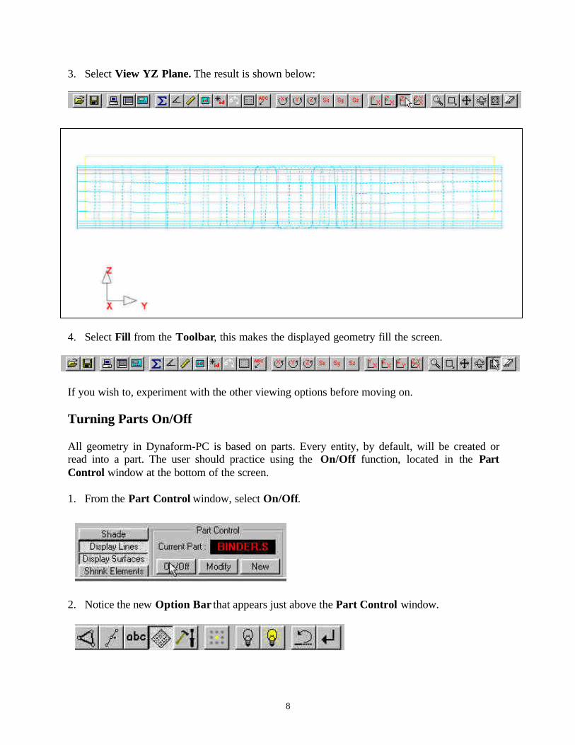
3. Select View YZ Plane. The result is shown below:

4. Select Fill from the Toolbar, this makes the displayed geometry fill the screen.

If you wish to, experiment with the other viewing options before moving on.

Turning Parts On/Off

All geometry in Dynaform-PC is based on parts. Every entity, by default, will be created orread into a part. The user should practice using the On/Off function, located in the PartControl window at the bottom of the screen.

1. From the Part Control window, select On/Off.

2. Notice the new Option Bar that appears just above the Part Control window.

9

This is the standard type of prompt Dynaform uses. Almost every function within thesoftware will bring up a similar bar. Hover over the different icons to learn the name of eachfunction. In the case of turning parts on and off, this bar gives you different ways of selectingwhat parts to turn on, and what parts to turn off.

3. Since the part BLANK.LIN has been generated using lines, you will have to use either theSelect by Line or the Select by Name function.

4. First, use the Select by Line option to turn off the part, BLANK.LIN. Click on the Select byLine icon, then select a line in the part, BLANK.LIN. This part will be turned off.

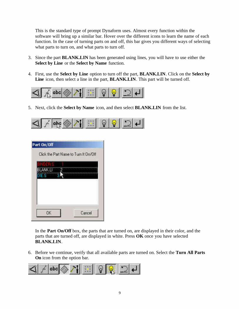
5. Next, click the Select by Name icon, and then select BLANK.LIN from the list.

In the Part On/Off box, the parts that are turned on, are displayed in their color, and theparts that are turned off, are displayed in white. Press OK once you have selectedBLANK.LIN.

6. Before we continue, verify that all available parts are turned on. Select the Turn All PartsOn icon from the option bar.

10

7. After you have turned all the parts on, click the End Select icon on the option bar. This willend the current operation.

Editing Parts in the Database

The Modify command, located in the Parts Control window is used to define and edit partproperties.

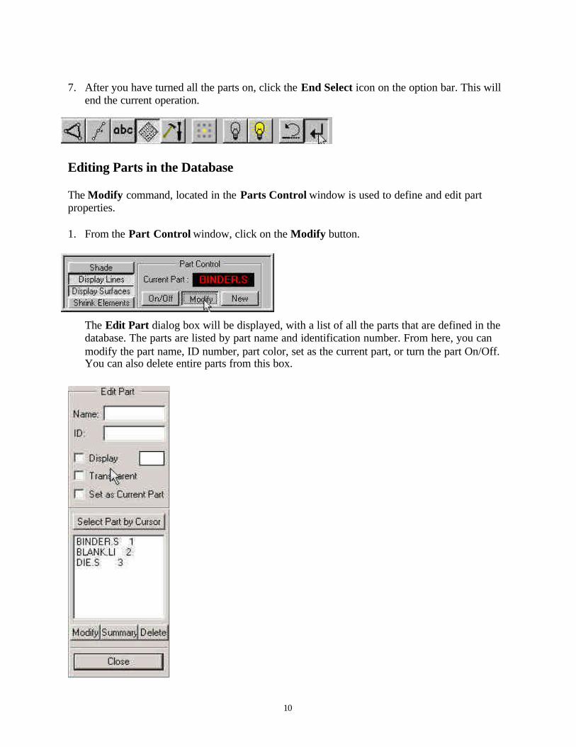
1. From the Part Control window, click on the Modify button.

The Edit Part dialog box will be displayed, with a list of all the parts that are defined in thedatabase. The parts are listed by part name and identification number. From here, you canmodify the part name, ID number, part color, set as the current part, or turn the part On/Off.You can also delete entire parts from this box.

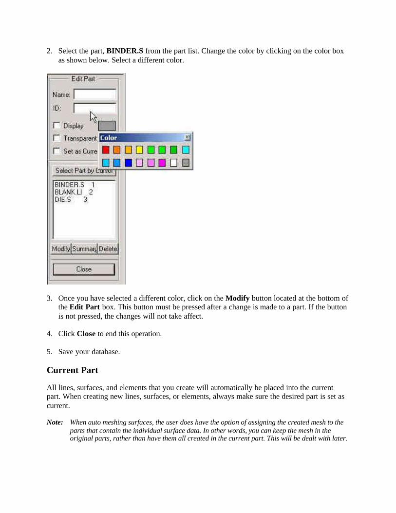
2. Select the part, BINDER.S from the part list. Change the color by clicking on the color boxas shown below. Select a different color.

3. Once you have selected a different color, click on the Modify button located at the bottom ofthe Edit Part box. This button must be pressed after a change is made to a part. If the buttonis not pressed, the changes will not take affect.

4. Click Close to end this operation.

5. Save your database.

Current Part

All lines, surfaces, and elements that you create will automatically be placed into the currentpart. When creating new lines, surfaces, or elements, always make sure the desired part is set ascurrent.

Note: When auto meshing surfaces, the user does have the option of assigning the created mesh to theparts that contain the individual surface data. In other words, you can keep the mesh in theoriginal parts, rather than have them all created in the current part. This will be dealt with later.

12

1. To change the current part, click on the Current Part box in the Part Control window.

2. An Option Bar will be displayed.

3. Similar to the On/Off option bar, this option bar allows you to select the current part indifferent ways. Hover over each icon to identify its function.

4. Set the part BLANK.LI as current by selecting the abc icon from the Option Bar.

5. Now, select the part, BLANK.LI from the Select a Part box that is displayed. Press OK andthe current part will be set.

6. Practice setting the current part as much as you would like. When you are done, turn off allof the parts except BLANK.LI, and set it as current.

13

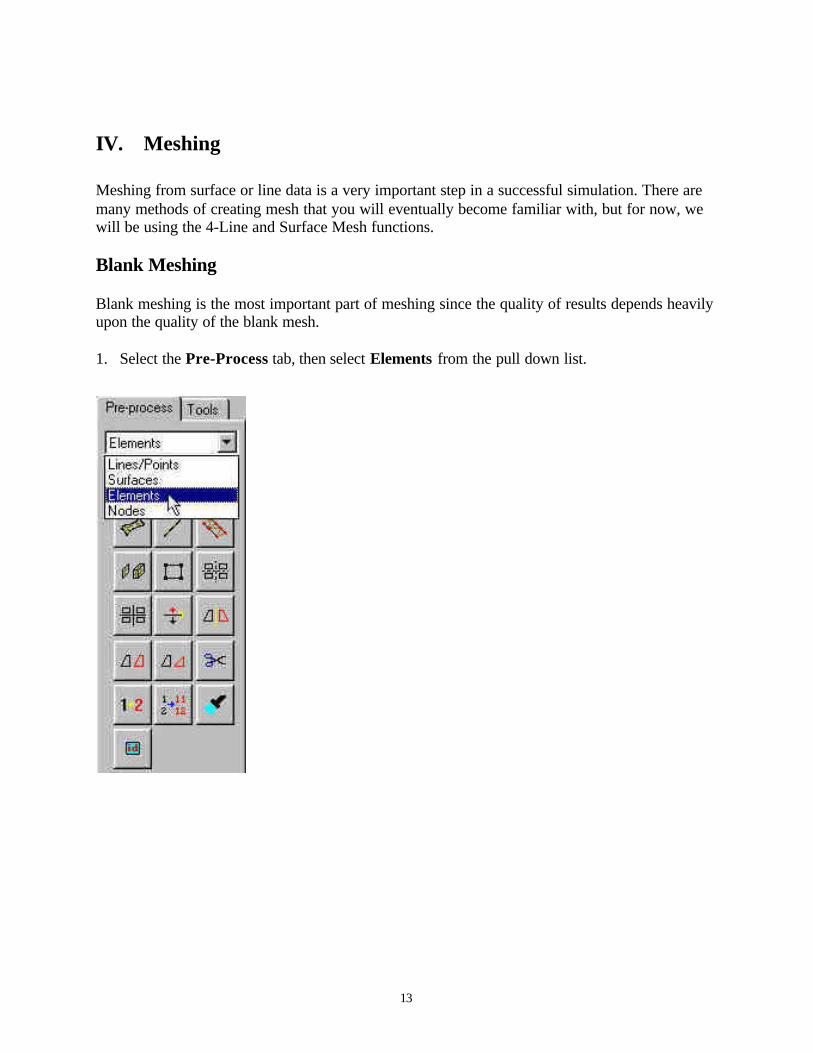
IV. Meshing

Meshing from surface or line data is a very important step in a successful simulation. There aremany methods of creating mesh that you will eventually become familiar with, but for now, wewill be using the 4-Line and Surface Mesh functions.

Blank Meshing

Blank meshing is the most important part of meshing since the quality of results depends heavilyupon the quality of the blank mesh.

1. Select the Pre-Process tab, then select Elements from the pull down list.

14

2. Select the 4-Line Mesh icon from the Pre-Process/Elements menu.

3. When you click the 4-Line Mesh button, a new Option Bar will be displayed, promptingyou to select the desired lines.

4. Make sure the Line option is highlighted (as in the picture above) and select the 4 lines thatmake up the blank in either a clockwise or counterclockwise order.

5. A dialog box prompts you to “ENTER THE NO. OF DIVISIONS ALONG EACH LINE:L1, L2, L3, and L4”

15

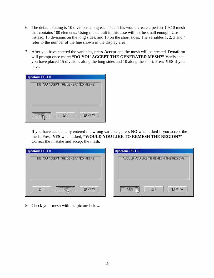
6. The default setting is 10 divisions along each side. This would create a perfect 10x10 meshthat contains 100 elements. Using the default in this case will not be small enough. Useinstead, 15 divisions on the long sides, and 10 on the short sides. The variables 1, 2, 3 and 4refer to the number of the line shown in the display area.

7. After you have entered the variables, press Accept and the mesh will be created. Dynaformwill prompt once more; “DO YOU ACCEPT THE GENERATED MESH?” Verify thatyou have placed 15 divisions along the long sides and 10 along the short. Press YES if youhave.

If you have accidentally entered the wrong variables, press NO when asked if you accept themesh. Press YES when asked, “WOULD YOU LIKE TO REMESH THE REGION?”Correct the mistake and accept the mesh.

8. Check your mesh with the picture below.

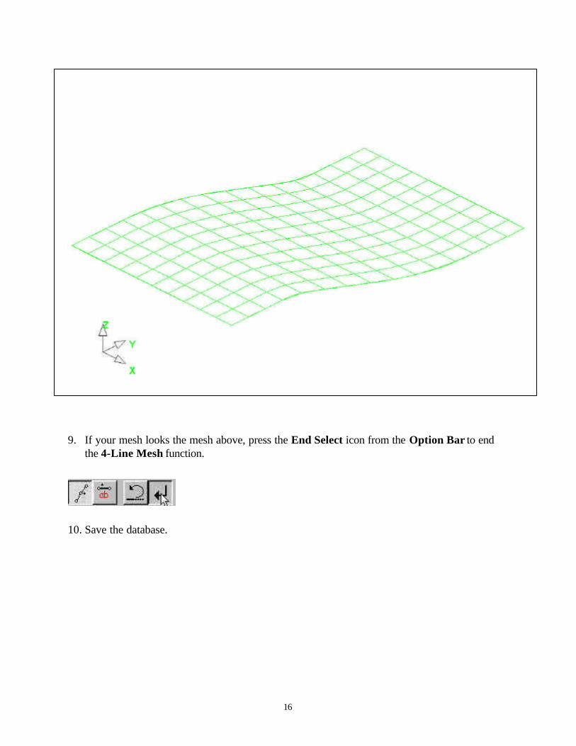
16

9. If your mesh looks the mesh above, press the End Select icon from the Option Bar to endthe 4-Line Mesh function.

10. Save the database.

17

Auto-Meshing Surface DataMost of the meshing done in Dynaform is done using the Surface Mesh function. This functionwill automatically create a mesh based on surface data that you provide. This is a very quick andeasy way of meshing the tools.

1. Turn off the part BLANK.LI and turn on the part BINDER.S. Set the part BINDER.S ascurrent.

2. Select Surface Mesh from the Pre-Process/Elements menu.

3. From the Option Bar, choose the Select Displayed Surfaces icon.

Notice all of the displayed surfaces will turn white. This verifies they have been selected.

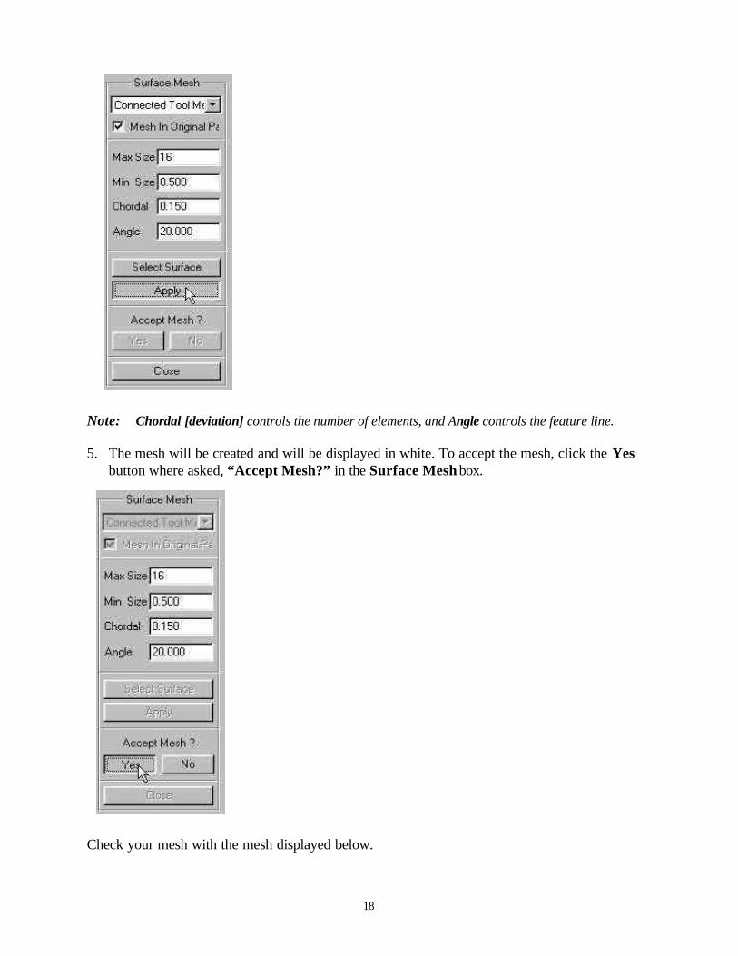
4. In the Surface Mesh dialogue that is displayed, edit the Max Size field to be 16. The defaultvalues will be used for the remaining fields. Be sure that the Mesh in Original Part option ischecked and click Apply.

18

Note: Chordal [deviation] controls the number of elements, and Angle controls the feature line.

5. The mesh will be created and will be displayed in white. To accept the mesh, click the Yesbutton where asked, “Accept Mesh?” in the Surface Mesh box.

Check your mesh with the mesh displayed below.

19

6. Press Close on the Surface Mesh box to end the function.

Auto-Meshing the Die Surface Data

1. Turn off all parts except for DIE.S and make it current.

2. Follow the previous 6 steps to auto-mesh the part DIE.S using 16 as the Max Size , 1 as theMin Size , and 0.005 as the Chordal Deviation.

3. Once you have generated the mesh with the given variables, close the Surface Mesh box andswitch to the isometric view and verify that your mesh looks like the mesh shown below.

20

4. Now that we have all the parts meshed, you can turn off the surfaces and lines in the PartControl box. This makes things easier to view the mesh. Save the changes.

V. Model Checking

Now that the mesh has been created, it needs to be checked in order to verify that there are notany defects that could cause problems later.

All the utilities you will be using to check the mesh are located under the check menu on themenu bar.

Click to deselect

21

Auto Plate Normal

1. Select Auto Plate Normal from the Check menu. A new Option Bar will be displayed.

2. This prompt is asking you to pick an element to identify a part to be checked for consistencyin the normal direction. Select an element on the part DIE.S. An arrow will displayedshowing the normal direction of the selected element. A prompt will ask “IS NORMALDIRECTION ACCEPTABLE?”

Pressing YES will check all elements in the part and reorient as needed to the direction thatis displayed. Pressing NO will check all elements and reorient as needed to the opposite ofthe direction that is displayed. In other words, press YES if you want the normal to point inthe direction of the displayed arrow, or NO if you want it to be the opposite. Since we will beusing the normal offset function to create the punch, set the normal direction to the negativeZ direction.

22

3. Now that the DIE.S elements are consistent you should check the rest of the parts in thedatabase. Turn off all the parts and turn each one on by itself. Check the normal direction andmake sure it is consistent.

Note: For the remaining parts, the direction of the normal does not matter because we will not be usingthe normal offset option on them. You will only need to verify that the directions are consistent.So, just select YES when asked if you accept the direction.

4. Once all the normal directions are consistent, turn on all of the parts and save the changes.

Display Model Boundary

This function will check the mesh for any gaps or holes, and highlight them so you can manuallycorrect the problem.

1. Select CheckÜÜDisplay Model BoundaryÜÜMultiple Surface.

2. There should not be any gaps in any of the meshes. Select the isometric view and make surethat your display looks like the one shown below.

23

3. Now, turn off all of the parts and notice that the boundary lines are still displayed. Thisallows you to inspect for any small gaps that might be hard to see with all of the meshesshowing. The results are shown below.

24

4. Turn only the part DIE.S back on and press the Clear button on the Toolbar to remove theboundary lines.

5. Save the database.

VI. Offsetting the Die Mesh to Create the Punch

Now that the normal direction is set in the correct direction (negative Z), and we have checkedfor gaps in the mesh, we are ready to offset the Die mesh to create the Punch.

1. The first thing you need to do is create a new part called PUNCH. This part will hold theelements that we offset from the die. Click the New button in the Part Control window.

2. In the New Part box, enter “PUNCH” in the name field and be sure that the options, Set asCurrent Part and Display, are checked. Click Create and the part will be created.

The part PUNCH has been created and we can now offset into this part.

25

3. Select the Copy Elements icon from the Pre-Process\Elements menu.

4. An option bar will be displayed, prompting you to select the elements that will be offset. Youwant to select all of the elements that make up the U-Channel of the part DIE.S. The easiestway to do this is to switch the view to the ZX plane on the Tool Bar, and then use the Selectby Drag Window function on the Option Bar.

Refer to the picture below.

26

5. After you have drawn a drag window and selected the elements, Dynaform will ask you,“DO YOU ACCEPT THE CURRENT DRAG WINDOW?” Confirm that you haveselected the correct region and press YES. If you have made a mistake, press NO and redrawthe drag window.

6. After pressing YES, you will notice that the selected elements will turn white. Verify oncemore that these are the correct elements by checking your display with the display shownbelow.

27

7. Press End Select after you have verified that the correct elements have been selected.

8. Enter 1 as the number of copies and press Accept.

28

9. Select Normal Offset as the transformation option and press Accept.

10. Enter the offset thickness. In Dynaform, we use the material thickness of the blank plus 10%.Since we will be using a blank thickness of 1, enter 1.1 in the box and press Accept.

Note: We use 10% of the thickness for simulation because when we do the post-processing, sometimeswrinkle data is lost if there is not enough space between the punch and die after it has completedits travel path. If we use only the blank thickness as a gap, the punch will iron the blank, creatingthe impression that no wrinkling has occurred.

11. Dynaform will ask you, “INCLUDE ELEMENT IN ITS ORIGINAL PART?” SelectingYES will place all of the offset elements into the part DIE.S, pressing NO will place all ofthe elements in the current part. Make sure PUNCH is set as current, and press NO.

29

12. Check your display with the display below. If your results differ, Right Click in the DisplayArea and press Undo Last. Repeat the above steps to re-offset.

30

13. Turn off the part DIE.S so that only PUNCH is displayed. Switch to the isometric view.Check your display with the display below.

14. Save the changes.

V. Tool Definition

Defining Parts as Tools

The parts BINDER.S, DIE.S, BLANK.LI, and PUNCH are all meshed and can now be definedas tools. After the parts have been defined as tools, we will setup the analysis parameters andstart the solver.

1. Switch to the Tools Menu and select the Define Tools icon.

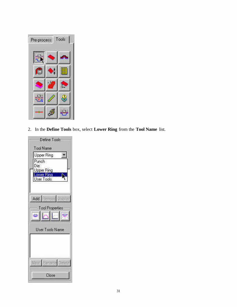
31

2. In the Define Tools box, select Lower Ring from the Tool Name list.

32

3. Press Add.

4. A new Option Bar will be displayed, prompting you to select which part will be defined asthe Lower Ring. Choose the Select by Name (abc) icon.

5. From the Select Multiple Parts box that is displayed, select BINDER.S and then press OK.

6. Press the End Select icon and the part BINDER.S will be defined as the Lower Ring.

7. Repeat the above steps to define the Punch and Die. Remember to select the correct ToolName in Step 2.

33

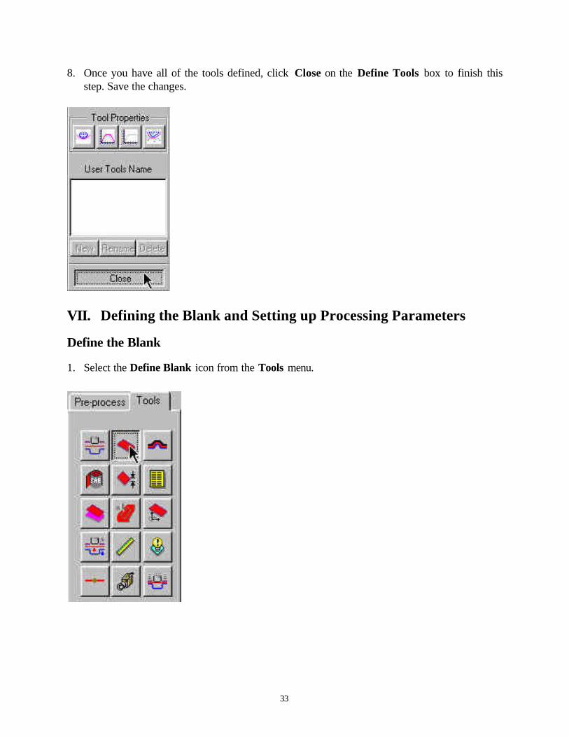
8. Once you have all of the tools defined, click Close on the Define Tools box to finish thisstep. Save the changes.

VII. Defining the Blank and Setting up Processing Parameters

Define the Blank

1. Select the Define Blank icon from the Tools menu.

34

2. Press Add in the Define Blank box.

3. A new Option Bar is displayed. Choose the Select by Name icon.

4. Select BLANK.LI from the Select Multiple Parts box and press OK.

5. Press End Select on the Option Bar and the Blank will be defined.

35

Defining the Blank Material

1. The Define Blank box should still be opened, click on the button just below where it saysMaterial: (This button will say None because the material has not been defined yet).

2. In the Define Material box, enter a name for the material, or use the default. From theMaterial Type list, be sure type 36 is selected and click Add.

36

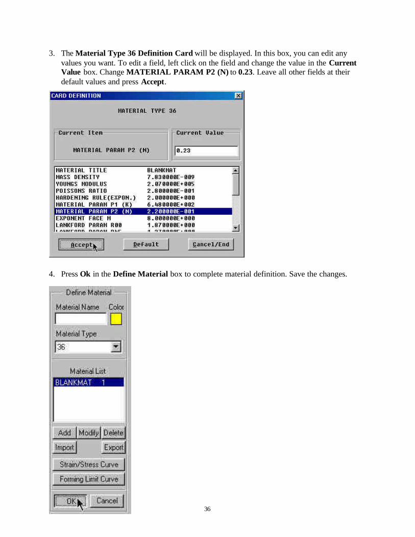
3. The Material Type 36 Definition Card will be displayed. In this box, you can edit anyvalues you want. To edit a field, left click on the field and change the value in the CurrentValue box. Change MATERIAL PARAM P2 (N) to 0.23. Leave all other fields at theirdefault values and press Accept.

4. Press Ok in the Define Material box to complete material definition. Save the changes.

37

Define Blank Property

1. The Define Blank box should still be opened, click on the button just below where it saysProperty: (This button will say None because the property has not been defined yet).

2. In the Define Property box, enter a name for the material, or use the default. Be sureBelytschko-Tsay is selected as the formulation type, and click Add.

38

3. The Belytschko-Tsay Definition Card will be displayed. Use the default values for all ofthe listed parameters except for the Uniform Thickness. Edit the Uniform Thickness to be1 and press Accept.

4. Press Ok in the Define Property box to complete property definition. Save the changes.

39

5. With both the blank material and blank property defined, you can now press Close in theDefine Blank window to end blank definition.

Tools Summary

1. You can verify that you have defined all of the needed tools by selecting the ToolsSummary function on the Tools menu.

40

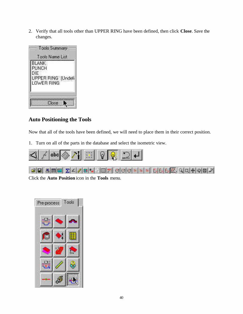
2. Verify that all tools other than UPPER RING have been defined, then click Close. Save thechanges.

Auto Positioning the Tools

Now that all of the tools have been defined, we will need to place them in their correct position.

1. Turn on all of the parts in the database and select the isometric view.

Click the Auto Position icon in the Tools menu.

41

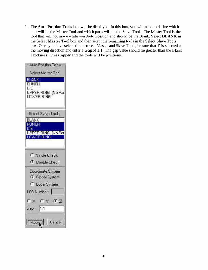
2. The Auto Position Tools box will be displayed. In this box, you will need to define whichpart will be the Master Tool and which parts will be the Slave Tools. The Master Tool is thetool that will not move while you Auto Position and should be the Blank. Select BLANK inthe Select Master Tool box and then select the remaining tools in the Select Slave Toolsbox. Once you have selected the correct Master and Slave Tools, be sure that Z is selected asthe moving direction and enter a Gap of 1.1 (The gap value should be greater than the BlankThickness). Press Apply and the tools will be positions.

42

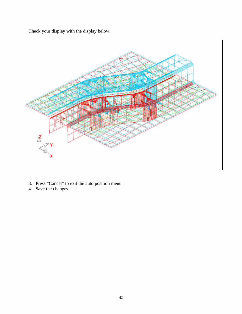
Check your display with the display below.

3. Press “Cancel” to exit the auto position menu.4. Save the changes.

43

Measuring the Punch Moving Distance

Now that the meshes have been created and the parts have been defined as tools, we can setupthe motion curves. The first step will be to find the moving distances for the parts.

1. Select the Min. Distance icon from the Tools menu.

2. The Min. Distance box will be displayed. Select Z as the direction to measure in, thenhighlight Punch, then Die. This will measure the distance, in the Z-direction, between thePunch and the Die, and display it in the Distance box.

44

3. The total distance between the Punch and the Die is approximately 42.2. To find the Punchtravel distance, subtract the Blank thickness + 10% of the Blank thickness. After doing so,we get a Punch travel distance of approximately 41.1. Take note of the number you get.

Note: We use 10% of the thickness for simulation because when we do the post-processing, sometimeswrinkle data is lost if there is not enough space between the punch and die after it has completedits travel path. If we use only the blank thickness as a gap, the punch will iron the blank, creatingthe impression that no wrinkling has occurred.

4. You can now press Close in the Min. Distance box, and end this step.

45

Define Punch Velocity Curve

1. From the Tools Menu, select the Define Tools icon.

2. Select Punch in the Tool Name list and then select the Define Motion Curve icon.

46

3. Select Z on the bottom of the Tool Motion Curve box to define the moving direction, thenpress Auto.

4. Use the default Curve Type (Tropezoidal) and keep the begin time of 0.000E+000. In theVelocity field, enter 8000 (this is in mm per second). For the Stroke Dist., use the value thatwe found after measuring the Punch travel distance and subtracting the Blank thickness +10%. The value should be approximately 41.1. Once you have entered the values, press Yesand a new Velocity vs. Distance motion curve will be created and displayed.

47

5. Verify that your graph is identical to the graph shown below.

6. Press Ok in the Curve Show Property box to return to the Tool Motion Curve box. Fromhere, press Ok once more to return to the Define Tools box. Do not close this box, the nextstep will start from here.

48

Defining Lower Ring (Binder) Force Curve

Now that the Punch travel curve has been created, we can create the force curve for the LowerRing.

1. From the Define Tools box, select Lower Ring from the Tool Name menu and select theDefine Force Curve icon.

2. In the Tool Force Curve box, select Z to define the moving direction and then press Auto.

49

3. Enter 200000 (N) in the FORCE and press Create.

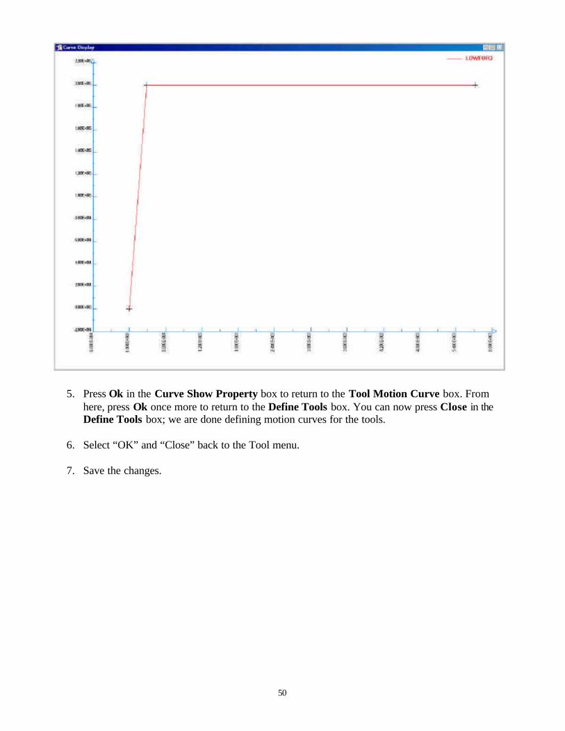
4. The Lower Ring force curve will be displayed. Verify that it is identical to the curve shownbelow.

50

5. Press Ok in the Curve Show Property box to return to the Tool Motion Curve box. Fromhere, press Ok once more to return to the Define Tools box. You can now press Close in theDefine Tools box; we are done defining motion curves for the tools.

6. Select “OK” and “Close” back to the Tool menu.

7. Save the changes.

51

Preview Tool Animation

We have now completed all of the pre-processing outside of setting up the final simulationparameters and submitting the job. Before we can do that however, we should verify that thetools are moving correctly, based on the motion curve information we have provided.

1. Select the Tools Animate icon from the Tools menu.

2. You will be prompted to “Please Enter Number of Frames (1~20)”. Accept the defaultvalue of 10 frames.

Note: Depending on the speed of the machine you are running Dynaform on, the animation mightmove too quickly. If this is the case, enter a larger number of frames.

52

3. You can change the view while running the preview animation. Also, notice the framecontrols on the Option Bar. Verify that the Punch is moving in the Z-direction, and makesure it is moving the full distance into the Die. Since we are using a force curve for theBinder, you will not see it move. When you are done viewing the animation, press the EndSelect button on the Option Bar.

4. Save the database.

VIII. Running the Analysis

Now that we have verified that the tool motion is correct, we can define the final parameters andrun the analysis.

Running the Analysis with Adaptive Mesh

Adaptive mesh allows for more accurate results by re-meshing the model as needed. In otherwords, when the solver comes across an area on the Die that will demand a finer mesh to capturethe geometry, it will split the original mesh to create finer, smaller elements.

1. Select AnalysisÜÜRun LS-DYNA… from the Menu Bar.

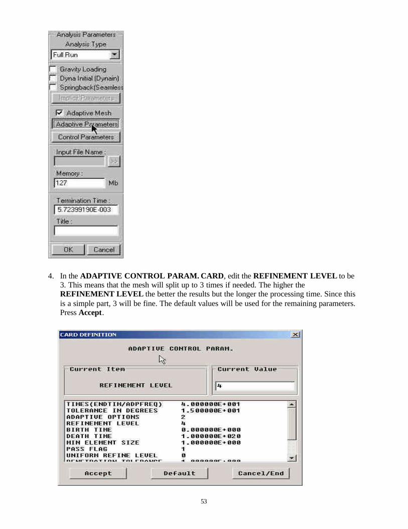
2. The Analysis Parameters box will be displayed. Turn on Adaptive mesh by clicking thecheck box.

3. Select the Adaptive Parameters button as shown below.

53

4. In the ADAPTIVE CONTROL PARAM. CARD, edit the REFINEMENT LEVEL to be3. This means that the mesh will split up to 3 times if needed. The higher theREFINEMENT LEVEL the better the results but the longer the processing time. Since thisis a simple part, 3 will be fine. The default values will be used for the remaining parameters.Press Accept.

54

5. Now, click the Control Parameters button in the Analysis Parameters box.

6. As a new user it is recommended that you use the default control parameters. So, pressDefault, then Accept.

55

7. The job is ready to run. Be sure that Full Run is selected from the Analysis Type menu andpress Ok. The Job will begin to run.

8. The solver is now running. You will notice that an estimated completion time is given. Thistime is not totally accurate since we are using adaptive mesh and the model will re-meshseveral times. However, it does give you a ballpark idea.

EstimatedTime

56

9. Once the solver has given you the preliminary estimated time, you can refresh this value byfirst pressing Ctrl-C. This will momentarily pause the solver and prompt you to “.entersense switch:” Then, enter the switch you would like to use and press enter:

Enter sw2 and press Enter. Notice the estimated time has changed. You can use theseswitches at anytime while the solver is running.

When you submit a job in Dynaform, an input deck is created which the solver, LS-DYNA, usesto process the results. The default input deck names are lsdynainput.dyn and lsdynainput.mod.The .dyn file contains all of the control cards, and the .mod file contains the geometry data.Advanced users are encouraged to study the .dyn input file. For more information, refer to theLS-DYNA User’s Manual (LS-DYNA.pdf) located in C:\Program Files\eta\Dynaform\Manuals.

Note: All files generated by either Dynaform or LS-DYNA will be placed in the directory in which theDynaform database has been saved. This includes all input decks and post processing files.

sw1 – Terminates the Solver

sw2 – Refreshes the Estimated Solving Time

sw3 – Creates a d3dump Restart File

sw4 – Creates a d3plot File

Note: These switches are case sensitive andmust be all lower case when entered.

57

LS-DYNA Input File Generated using DYNAFORM-PC:

$ ETA/DYNAFORM : LS-DYNA(950) INPUT DECK$ DATE : Dec 18, 2000 at 16:36:16$$ VIEWING INFORMATION$ -.171154E+02 .345210E+03-.119772E+03 .132504E+03$ .707100E+00 .707100E+00 .000000E+00$ -.353550E+00 .353550E+00 .866020E+00$ .612370E+00-.612370E+00 .500000E+00$$ DRAW INFORMATION$ DRAWTYPE DIRECTION BEADTYPE POSITION$ 2 3 1 1.000$$---+----1----+----2----+----3----+----4----+----5----+----6----+----7----+----8$*KEYWORD$$---+----1----+----2----+----3----+----4----+----5----+----6----+----7----+----8$$ (1) TITLE CARD.$$---+----1----+----2----+----3----+----4----+----5----+----6----+----7----+----8*TITLENONE$---+----1----+----2----+----3----+----4----+----5----+----6----+----7----+----8$$ (2) CONTROL CARDS.$$---+----1----+----2----+----3----+----4----+----5----+----6----+----7----+----8$*CONTROL_STRUCTURED_TERM*CONTROL_TERMINATION$ ENDTIM ENDCYC DTMIN ENDENG ENDMAS0.00572400 0 .000*CONTROL_TIMESTEP$ DTINIT TSSFAC ISDO TSLIMT DT2MS LCTM ERODEMS1ST .000 .900 0 .000-1.635E-07*CONTROL_HOURGLASS$ IHQ QH 4 .100*CONTROL_BULK_VISCOSITY$ Q1 Q2 TYPE 1.500 .060 1*CONTROL_SHELL$ WRPANG ITRIST IRNXX ISTUPD THEORY BWC MITER 20.000 2 -1 1 2 2 1*CONTROL_CONTACT$ SLSFAC RWPNAL ISLCHK SHLTHK PENOPT THKCHG ORIEN

58

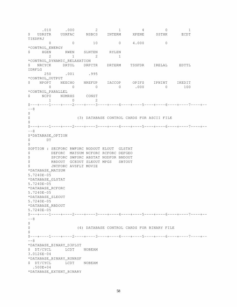
.010 .000 2 1 4 0 1$ USRSTR USRFAC NSBCS INTERM XPENE SSTHK ECDTTIEDPRJ 0 0 10 0 4.000 0*CONTROL_ENERGY$ HGEN RWEN SLNTEN RYLEN 2 1 2 1*CONTROL_DYNAMIC_RELAXATION$ NRCYCK DRTOL DRFCTR DRTERM TSSFDR IRELAL EDTTLIDRFLG 250 .001 .995*CONTROL_OUTPUT$ NPOPT NEECHO NREFUP IACCOP OPIFS IPNINT IKEDIT 0 0 0 0 .000 0 100*CONTROL_PARALLEL$ NCPU NUMRHS CONST 1 0 2$---+----1----+----2----+----3----+----4----+----5----+----6----+----7----+----8$$ (3) DATABASE CONTROL CARDS FOR ASCII FILE$$---+----1----+----2----+----3----+----4----+----5----+----6----+----7----+----8$*DATABASE_OPTION$ DT$$OPTION : SECFORC RWFORC NODOUT ELOUT GLSTAT$ DEFORC MATSUM NCFORC RCFORC DEFGEO$ SPCFORC SWFORC ABSTAT NODFOR BNDOUT$ RBDOUT GCEOUT SLEOUT MPGS SBTOUT$ JNTFORC AVSFLT MOVIE*DATABASE_MATSUM5.7240E-05*DATABASE_GLSTAT5.7240E-05*DATABASE_RCFORC5.7240E-05*DATABASE_SLEOUT5.7240E-05*DATABASE_RBDOUT5.7240E-05$---+----1----+----2----+----3----+----4----+----5----+----6----+----7----+----8$$ (4) DATABASE CONTROL CARDS FOR BINARY FILE$$---+----1----+----2----+----3----+----4----+----5----+----6----+----7----+----8*DATABASE_BINARY_D3PLOT$ DT/CYCL LCDT NOBEAM3.0126E-04*DATABASE_BINARY_RUNRSF$ DT/CYCL LCDT NOBEAM .500E+04*DATABASE_EXTENT_BINARY

59

$ NEIPH NEIPS MAXINT STRFLG SIGFLG EPSFLG RLTFLGENGFLG 5 1$ CMPFLG IEVERP BEAMIP DCOMP SHGE STSSZ 1 2$---+----1----+----2----+----3----+----4----+----5----+----6----+----7----+----8$$ (5) DEFINE TOOLS IN DYNAFORM$$---+----1----+----2----+----3----+----4----+----5----+----6----+----7----+----8$ BLANK DESCRIPTION$---+----1----+----2----+----3----+----4----+----5----+----6----+----7----+----8*SET_PART_LIST$SET_PART_NAME: BLANK$ SID DA1 DA2 DA3 DA4 1$ PID1 PID2 PID3 PID4 PID5 PID6 PID7PID8 2*PART$HEADING PART PID = 2 PART NAME :BLANK.LI$ PID SECID MID EOSID HGID GRAV ADPOPT 2 6 1 1*MAT_3-PARAMETER_BARLAT$MATERIAL NAME:BLANKMAT$ MID RO E PR HR P1 P2 1 7.830E-09 2.070E+05 2.800E-01 2.000E+00 6.480E+02 2.300E-01$ M R00 R45 R90 LCID E0 SPI 8.000E+00 1.870E+00 1.270E+00 2.170E+00 0 0.000E+00 0.000E+00$ AOPT 2.0$ XP YP ZP A1 A2 A3 1.000E+00 0.000E+00 0.000E+00$ V1 V2 V3 D1 D2 D3 0.000E+00 1.000E+00 0.000E+00*SECTION_SHELL$PROPERTY NAME:BLANKPRO$ SECID ELFORM SHRF NIP PROPT QR/IRID ICOMP 6 2 .830E+00 5.0 1.0 .0$ T1 T2 T3 T4 NLOC 1.000E+00 1.000E+00 1.000E+00 1.000E+00*CONTROL_ADAPTIVE$ ADPFREQ ADPTOL ADPOPT MAXLVL TBIRTH TDEATH LCADPIOFLAG1.4310E-04 .500E+01 2 30.0000e+001.0000E+201$ ADPSIZE ADPASS IREFLG ADPENE ADPTH MEMORY ORIENTMAXEL 1.000 1 0 1.000 .500 00$---+----1----+----2----+----3----+----4----+----5----+----6----+----7----+----8$ PUNCH DESCRIPTION

60

$---+----1----+----2----+----3----+----4----+----5----+----6----+----7----+----8*SET_PART_LIST$SET_PART_NAME: PUNCH$ SID DA1 DA2 DA3 DA4 2$ PID1 PID2 PID3 PID4 PID5 PID6 PID7PID8 5*PART$HEADING PART PID = 5 PART NAME :PUNCH$ PID SECID MID EOSID HGID GRAV ADPOPT 5 7 2*MAT_RIGID$MATERIAL NAME:PUNCHMAT$ MID RO E PR N COUPLE MALIAS 2 7.830E-09 2.070E+05 2.800E-01 0.000E+00 0.000E+00 0.000E+00$ CMO CON1 CON2 1.0 4.0 7.0$LCO or A1 A2 A3 V1 V2 V3

*SECTION_SHELL$PROPERTY NAME:PUNCHPRO$ SECID ELFORM SHRF NIP PROPT QR/IRID ICOMP 7 2 .100E+01 3.0 .0 .0$ T1 T2 T3 T4 NLOC .500E+00 .500E+00 .500E+00 .500E+00*CONTACT_FORMING_ONE_WAY_SURFACE_TO_SURFACE$ CID CONTACT INTERFACE TITLE$ 2 BLANK/PUNCH$ SSID MSID SSTYP MSTYP SBOXID MBOXID SPRMPR 1 2 2 2$ FS FD DC VC VDC PENCHK BTDT .125E+00 .000E+00 .000E+00 .000E+00 .200E+0200.0000e+001.0000E+20$ SFS SFM SST MST SFST SFMT FSFVSF .000E+00 .000E+00 .000E+00 .000E+00$ SOFT SOFSCL LCIDAB MAXPAR PENTOL DEPTH BSORTFRCFRQ 0$ PENMAX THKOPT SHLTHK SNLOG 1*BOUNDARY_PRESCRIBED_MOTION_RIGID$ PID DOF VAD LCID SF VID DEATH 5 3 0 1 1.0$---+----1----+----2----+----3----+----4----+----5----+----6----+----7----+----8$ DIE DESCRIPTION$---+----1----+----2----+----3----+----4----+----5----+----6----+----7----+----8*SET_PART_LIST$SET_PART_NAME: DIE

61

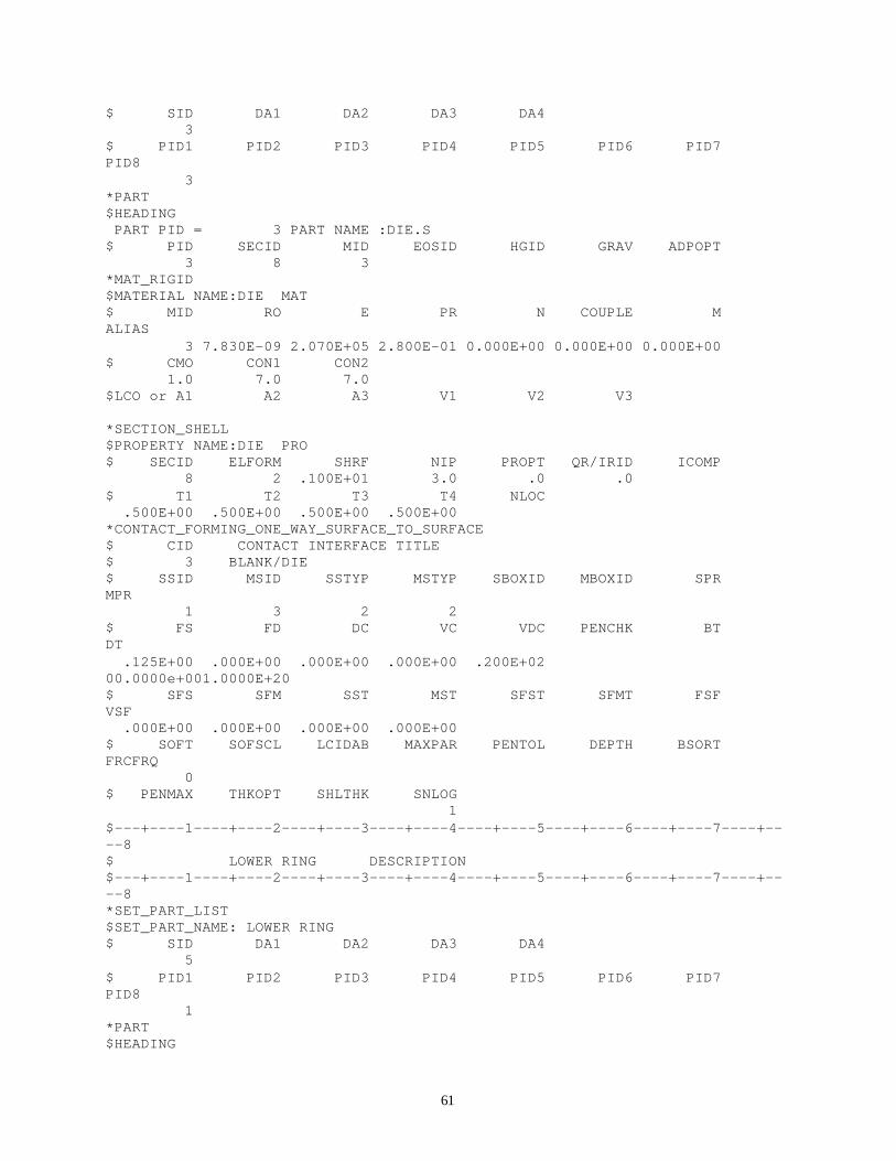
$ SID DA1 DA2 DA3 DA4 3$ PID1 PID2 PID3 PID4 PID5 PID6 PID7PID8 3*PART$HEADING PART PID = 3 PART NAME :DIE.S$ PID SECID MID EOSID HGID GRAV ADPOPT 3 8 3*MAT_RIGID$MATERIAL NAME:DIE MAT$ MID RO E PR N COUPLE MALIAS 3 7.830E-09 2.070E+05 2.800E-01 0.000E+00 0.000E+00 0.000E+00$ CMO CON1 CON2 1.0 7.0 7.0$LCO or A1 A2 A3 V1 V2 V3

*SECTION_SHELL$PROPERTY NAME:DIE PRO$ SECID ELFORM SHRF NIP PROPT QR/IRID ICOMP 8 2 .100E+01 3.0 .0 .0$ T1 T2 T3 T4 NLOC .500E+00 .500E+00 .500E+00 .500E+00*CONTACT_FORMING_ONE_WAY_SURFACE_TO_SURFACE$ CID CONTACT INTERFACE TITLE$ 3 BLANK/DIE$ SSID MSID SSTYP MSTYP SBOXID MBOXID SPRMPR 1 3 2 2$ FS FD DC VC VDC PENCHK BTDT .125E+00 .000E+00 .000E+00 .000E+00 .200E+0200.0000e+001.0000E+20$ SFS SFM SST MST SFST SFMT FSFVSF .000E+00 .000E+00 .000E+00 .000E+00$ SOFT SOFSCL LCIDAB MAXPAR PENTOL DEPTH BSORTFRCFRQ 0$ PENMAX THKOPT SHLTHK SNLOG 1$---+----1----+----2----+----3----+----4----+----5----+----6----+----7----+----8$ LOWER RING DESCRIPTION$---+----1----+----2----+----3----+----4----+----5----+----6----+----7----+----8*SET_PART_LIST$SET_PART_NAME: LOWER RING$ SID DA1 DA2 DA3 DA4 5$ PID1 PID2 PID3 PID4 PID5 PID6 PID7PID8 1*PART$HEADING

62

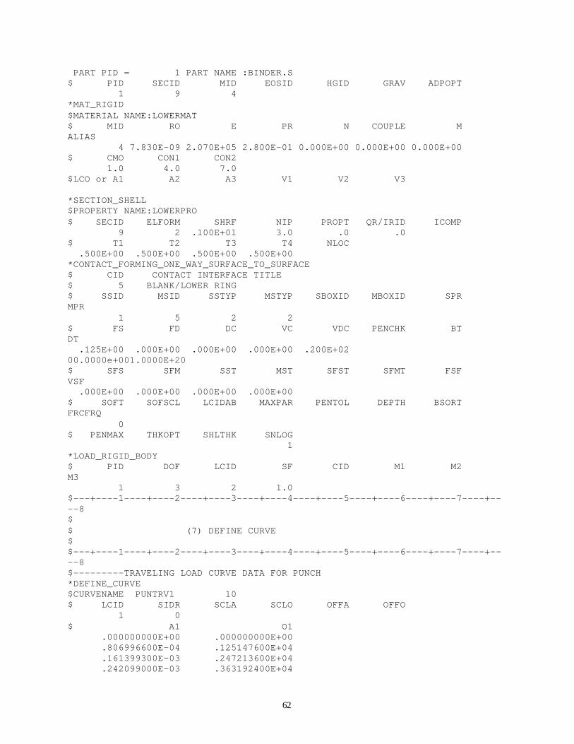
PART PID = 1 PART NAME :BINDER.S$ PID SECID MID EOSID HGID GRAV ADPOPT 1 9 4*MAT_RIGID$MATERIAL NAME:LOWERMAT$ MID RO E PR N COUPLE MALIAS 4 7.830E-09 2.070E+05 2.800E-01 0.000E+00 0.000E+00 0.000E+00$ CMO CON1 CON2 1.0 4.0 7.0$LCO or A1 A2 A3 V1 V2 V3

*SECTION_SHELL$PROPERTY NAME:LOWERPRO$ SECID ELFORM SHRF NIP PROPT QR/IRID ICOMP 9 2 .100E+01 3.0 .0 .0$ T1 T2 T3 T4 NLOC .500E+00 .500E+00 .500E+00 .500E+00*CONTACT_FORMING_ONE_WAY_SURFACE_TO_SURFACE$ CID CONTACT INTERFACE TITLE$ 5 BLANK/LOWER RING$ SSID MSID SSTYP MSTYP SBOXID MBOXID SPRMPR 1 5 2 2$ FS FD DC VC VDC PENCHK BTDT .125E+00 .000E+00 .000E+00 .000E+00 .200E+0200.0000e+001.0000E+20$ SFS SFM SST MST SFST SFMT FSFVSF .000E+00 .000E+00 .000E+00 .000E+00$ SOFT SOFSCL LCIDAB MAXPAR PENTOL DEPTH BSORTFRCFRQ 0$ PENMAX THKOPT SHLTHK SNLOG 1*LOAD_RIGID_BODY$ PID DOF LCID SF CID M1 M2M3 1 3 2 1.0$---+----1----+----2----+----3----+----4----+----5----+----6----+----7----+----8$$ (7) DEFINE CURVE$$---+----1----+----2----+----3----+----4----+----5----+----6----+----7----+----8$---------TRAVELING LOAD CURVE DATA FOR PUNCH*DEFINE_CURVE$CURVENAME PUNTRV1 10$ LCID SIDR SCLA SCLO OFFA OFFO 1 0$ A1 O1 .000000000E+00 .000000000E+00 .806996600E-04 .125147600E+04 .161399300E-03 .247213600E+04 .242099000E-03 .363192400E+04

63

.322798600E-03 .470228200E+04 .403498300E-03 .565685400E+04 .484198000E-03 .647213600E+04 .564897600E-03 .712805200E+04 .645597300E-03 .760845200E+04 .726297000E-03 .790150700E+04 .806996700E-03 .800000000E+04 .491699600E-02 .800000000E+04 .499769600E-02 .790150700E+04 .507839500E-02 .760845200E+04 .515909500E-02 .712805200E+04 .523979400E-02 .647213600E+04 .532049400E-02 .565685400E+04 .540119400E-02 .470228200E+04 .548189300E-02 .363192400E+04 .556259300E-02 .247213600E+04 .564329200E-02 .125147600E+04 .572399200E-02 .000000000E+00$---------FORCE LOAD CURVE DATA FOR LOWER RING*DEFINE_CURVE$CURVENAME LOWFOR2 11$ LCID SIDR SCLA SCLO OFFA OFFO 2 0$ A1 O1 .000000000E+00 .000000000E+00 .286200000E-03 .200000000E+06 .572400000E-02 .200000000E+06$---------OTHER CURVES$---+----1----+----2----+----3----+----4----+----5----+----6----+----7----+----8$$ MODEL DATA IN FILE :inputdyna.mod$ NUMBER OF NODES : 5475$ NUMBER OF SHELLS : 5511$*INCLUDEinputdyna.mod$$---+----1----+----2----+----3----+----4----+----5----+----6----+----7----+----8$---+----1----+----2----+----3----+----4----+----5----+----6----+----7----+----8$*END

64

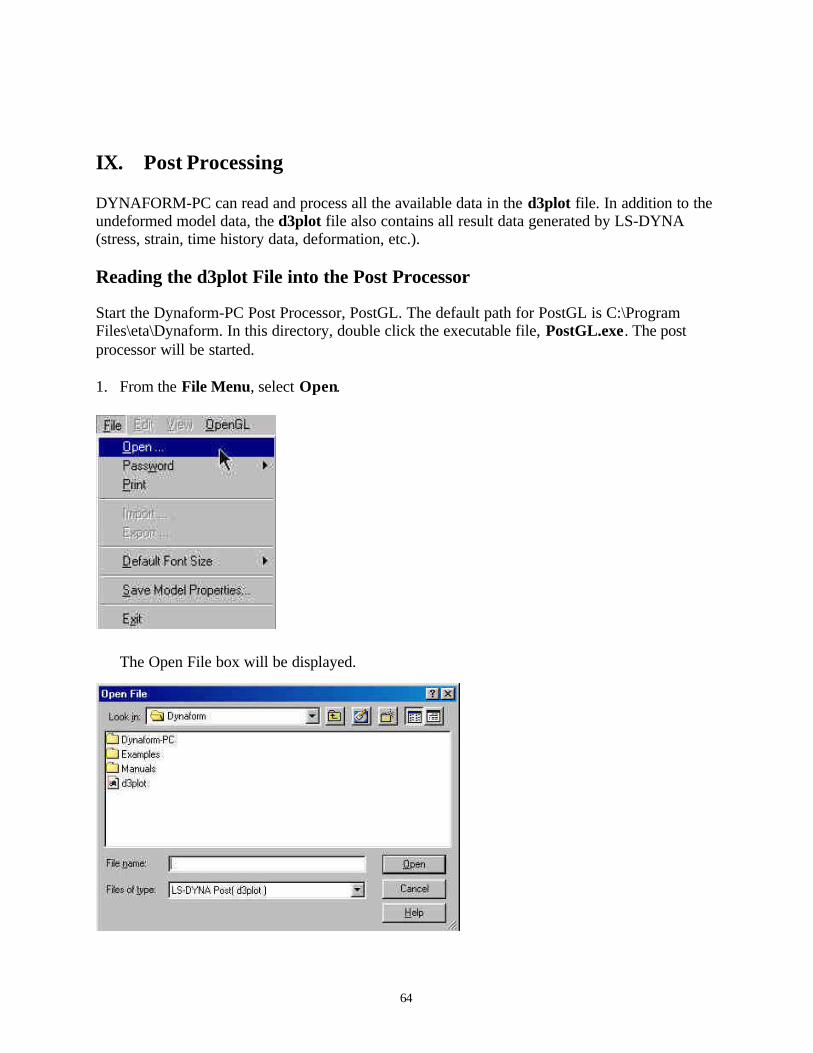
IX. Post Processing

DYNAFORM-PC can read and process all the available data in the d3plot file. In addition to theundeformed model data, the d3plot file also contains all result data generated by LS-DYNA(stress, strain, time history data, deformation, etc.).

Reading the d3plot File into the Post Processor

Start the Dynaform-PC Post Processor, PostGL. The default path for PostGL is C:\ProgramFiles\eta\Dynaform. In this directory, double click the executable file, PostGL.exe. The postprocessor will be started.

1. From the File Menu, select Open.

The Open File box will be displayed.

65

2. Select LS-DYNA Post (d3plot) to PP file from the Files of Type list. This option will allowyou to read in the d3plot file and then automatically create a file called PostGL.pp. The .ppfile can be read in much faster then the d3plot file, and allows you to save space, since the.pp file is much smaller then the d3plot files. You will only need to read in the d3plot fileonce. From then on, you should use the PostGL.pp file.

After moving to the directory where you saved the Dynaform database, be sure you have thecorrect file of type selected, pick the d3plot file, and press Open.

3. When prompted to “SELECT LS-DYNA VERSION”, select LS940/LS950 and press Ok.

66

4. When prompted to “SELECT TIME STEPS”, select ALL AVAILABLE STEPS and pressOk.

5. When prompted to “SELECT RESULT COMPONENTS”, select ALL ITEMS then andpress Ok.

6. The d3plot file is now completely read in. You are ready to animate the results.

67

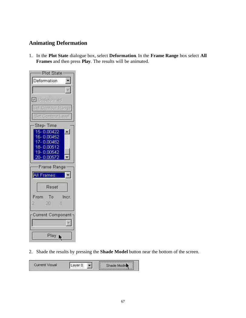
Animating Deformation

1. In the Plot State dialogue box, select Deformation. In the Frame Range box select AllFrames and then press Play. The results will be animated.

2. Shade the results by pressing the Shade Model button near the bottom of the screen.

68

3. Since it is difficult to see the Blank with all of the other tools displayed, you can turn them alloff, leaving only the Blank showing. In the Control Options box, select OFF/ON by Name .

4. Turn off all of the parts except for the Blank and press Ok.

69

5. You can also change the view with the view manipulation icons on the tool bar, just as wedid in the pre processor.

6. Try adjusting the frame rate by pressing the Frame Rate button in the Control Optionswindow. Sometimes this is necessary is the animation moves too quickly.

View Manipulation

70

7. You will be prompted to enter a new frame rate. Enter 5 and press Accept.

Notice the change in the speed of the animation. Adjust the frame rate until you find itacceptable.

8. Another way to control the speed of the animation is to advance or reverse frames manually.To do this, press either the Advance Frame or Reverse Frame button in the Control OptionsBox. Then move the mouse pointer into the display area and left-click. Notice the frames willadvance, or reverse, one at a time.

71

9. When you are done viewing the animation, press Stop in the Control Options box.

72

Animating Stresses/Strains and FLD

PostGL can also animate various stresses and strains as well as FLD. To do this, refer to thefollowing examples.

Stress/Strain

1. Pick Contour and Stress/Strain from the Plot State box.2. Select All Frames from the Frame Range menu.3. Select the type of Stress/Strain you would like to view from the Current Component list.

(The picture below has Thickness selected)4. Press Play and the animation will begin.

73

FLD

1. Pick FLD and On Element from the Plot State box.2. Select All Frames from the Frame Range menu.3. Select Middle from the Current Component list.4. Press Play and the animation will begin.

74

Plotting Single Frames

It is sometimes more convenient to view single frames rather than the entire animation To dothis, select Single Frame from the Frame Range box and then select, with your mouse, theframe you would like to view. Refer to the example below in which the FLD plot of the 17th

frame would be displayed upon pressing Plot.

75

Writing an AVI File

PostGL has a very useful tool that allows you to automatically create an avi movie via ananimation screen capture. This will be the last function covered in this training case.

1. Start a new animation using all available steps.2. Once the animation is running, click on the Write AVI File icon, located on the Toolbar.

3. The Write File box will be displayed. Enter a name to save the avi file under (e.g.traincase.avi), and press Save.

4. Enter a frame rate in the prompt box. It is recommended to use the default. Press Accept.

5. Enter a window size in the prompt box. It is recommended to use the default. Press Accept.

76

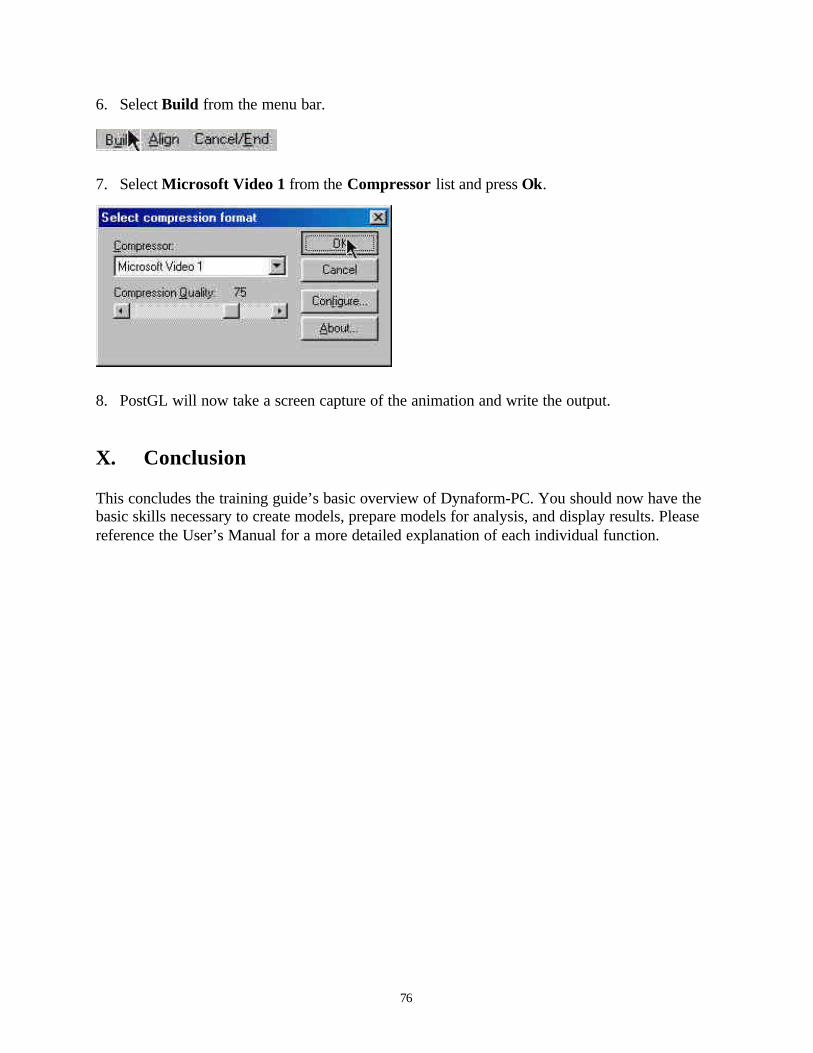
6. Select Build from the menu bar.

7. Select Microsoft Video 1 from the Compressor list and press Ok.

8. PostGL will now take a screen capture of the animation and write the output.

X. Conclusion

This concludes the training guide’s basic overview of Dynaform-PC. You should now have thebasic skills necessary to create models, prepare models for analysis, and display results. Pleasereference the User’s Manual for a more detailed explanation of each individual function.