psychometrika

doi: 10.1007/s11336-014-9406-0

HETEROSCEDASTIC LATENT TRAIT MODELS FOR DICHOTOMOUS DATA

Dylan Molenaar

UNIVERSITY OF AMSTERDAM

Effort has been devoted to account for heteroscedasticity with respect to observed or latent moderatorvariables in item or test scores. For instance, in the multi-group generalized linear latent trait model, itcould be tested whether the observed (polychoric) covariance matrix differs across the levels of an observedmoderator variable. In the case that heteroscedasticity arises across the latent trait itself, existing modelscommonly distinguish between heteroscedastic residuals and a skewed trait distribution. These modelshave valuable applications in intelligence, personality and psychopathology research. However, existingapproaches are only limited to continuous and polytomous data, while dichotomous data are common inintelligence and psychopathology research. Therefore, in present paper, a heteroscedastic latent trait modelis presented for dichotomous data. The model is studied in a simulation study, and applied to data pertainingalcohol use and cognitive ability.

Key words: heteroscedasticity, latent trait models, item response theory, two-parameter model,non-normal latent variables.

Generalized linear models constitute an important class of statistical tools in psychologicalresearch. The most obvious examples are MANOVA, the linear regression model, and the logitregression model used to test associations among observed variables. Other examples can befound in psychometrics, where generalized linear latent trait models like the common factormodel and the two-parameter model are used for psychological and educational measurement(see e.g. Mellenbergh, 1994a).

As a general rule in parametric statistical models, results can only be trusted to reflect aneffect that is actually present in the data if the assumptions underlying the statistical model are met.For the generalized linear models that are commonly used in psychology, a central assumption isthat of homoscedasticity (e.g. Dobson, 2010, p. 33; Greene, 2011). Homoscedasticity refers to therequirement that the variances of the random effects in a statistical model are constant across units(e.g. Green, 2011).1 In generalized linear modelling approaches, this requirement implies that theresidual covariance matrix does not differ across levels of the independent variables (Slutsky,1913; see Green, 2011 for the logit and probit case). If this assumption is violated, then onespeaks of heteroscedasticity.

Heteroscedasticity is a well-studied phenomenon within generalized linear models. Methodshave been proposed to test the equality of the residual covariance matrix across the levels of theindependent variables in MANOVA or t test type of analysis (e.g. Anderson, 2006), and methodshave been studied to account for possible violations (e.g. Brunner, Dette, & Munk, 1997). Inlinear regression models, various approaches exist to assess, test, or model heteroscedasticity,including diagnostic graphical approaches (e.g. Stevens, 2009, p. 90), statistical tests (e.g. Jarque& Bera, 1980), corrections (e.g. Long & Ervin, 2000), and approaches to model heteroscedasticityexplicitly (e.g. Harvey, 1976).

With respect to the generalized linear latent trait models in psychometrics, approaches tothe study of heteroscedasticity differ from those above as these models commonly contain an

Correspondence should be sent to Dylan Molenaar, Psychological Methods, Department of Psychology,University of Amsterdam, Weesperplein 4, 1018 XA Amsterdam, The Netherlands. E-mail: D.Molenaar@uva.nl

1 A sensible designation as ‘skedasis’ is the Greek word for scatter or dispersion.

© 2014 The Psychometric Society

PSYCHOMETRIKA

Table 1.Overview of models for heteroscedasticity within the generalized linear latent trait modelling framework.

Data Categorical moderator Continuous moderator

Manifest Latent Manifest Latent

Continuous Multi-group FM Factor Mixtures Moderated FM Heteroscedastic FMCategorical Multi-group IRT Mixture IRT Moderated IRT Heteroscedastic GRM

FM factor model, IRT item response theory, GRM graded response model.

additional random subject effect. That is, besides the variable-specific residual effect in the mea-surement model, there is a latent trait effect in the structural model that is common to all variables.Thus, for a given variable in a psychometric model, heteroscedasticity can have two sources. In theliterature, methods to model heteroscedasticity within the measurement and/or structural modelhave been studied elaborately for continuous and categorical data.2 See Table 1 for an overviewof the different approaches within the generalized linear latent trait framework. As can be seen,the methods are different in what they assume about the nature of the moderator variable acrosswhich the heteroscedasticity arises. In the case of heteroscedasticity with respect to a categoricalmoderator variable (or grouping variable), multi-group models (e.g. Jöreskog, 1971, Lee, Poon,& Bentler, 1989; Meredith, 1993; Muthén & Christoffersson, 1981) can be used to account fordifferences in the latent trait variance and the residual variances across the categories of a manifestmoderator (e.g. gender, see Dolan et al., 2006). In addition, mixture models (e.g. Dolan & Van derMaas, 1998; Jedidi, Jagpal, & DeSarbo, 1997; Mislevy & Verhelst, 1990; Rost, 1990) can be usedto test for differences in the latent trait variance and the residual variances across the categoriesof a latent moderator (i.e. latent to the data at hand; for instance stages of Piagetian conservation,see Jansen & Van der Maas, 1997).

Models that can be used in the case of heteroscedasticity with respect to a continuous moder-ator variable have been developed only recently for manifest moderators (e.g. Bauer & Hussong,2009; Mehta & Neale, 2005; Merkle & Zeileis, 2013; Neale, Aggen, Maes, Kubarych, & Schmitt,2006; Rabe-Hesketh, Skrondal, & Pickles, 2004). As the moderator is a continuous variable (e.g.age, see Molenaar, Dolan, Wicherts, & Van der Maas, 2010), the latent trait variance and/or theresidual variance are not estimated for each level of the moderator separately, but these parametersare made a parametric function of the continuous moderator. This approach can be consideredgeneralizations of the multi-group models as they include these models as special cases (see e.g.Bauer & Hussong, 2009). Note, however, that other approaches do not require the specificationof the exact form of the function between the variance parameters and the moderator (see Merkle& Zeileis, 2013; Merkle, Fan, & Zeileis, 2013).

In the case that the moderator is a latent continuous variable, the moderator variable andthe latent trait become indistinguishable and coincide. This implies that the heteroscedasticitycan only come about by residual variances that differ across the levels of the latent trait (Bollen,1996; Hessen & Dolan, 2009; Lewin-Koh & Amemiya, 2003; Meijer & Mooijaart, 1996). Asa skewed latent trait distribution can also result in unequal observed (polychoric) variances forhigh and low levels of the trait, this effect needs to be taken into account to disentangle the effectof heteroscedastic residuals from the non-normality of the trait distribution. The resulting modelis thus a latent trait model with heteroscedastic residuals and a skewed trait distribution, shortlydenoted by heteroscedastic latent trait model.

2 Truly continuous observed scores are rare in psychological and educational measurement. It has been shown thatpragmatically, a scale with 7 or more ordered levels can be treated as continuous (Dolan, 1994). Therefore, in this paper,the term ‘continuous variable’ is used to denote variables with 7 or more ordered levels.

DYLAN MOLENAAR

There are a number of reasons why studying this specific type of model is important (seeMolenaar, Dolan, & De Boeck, 2012, for a comprehensive discussion). First, as heteroscedasticresiduals result in asymmetric item characteristic curves, parameter bias may arise as has beenshown by Bazán, Branco, and Bolfarine (2006) and Molenaar et al. (2012). Second, Samejima(1997, 2000, 2008) demonstrated that symmetrical item characteristic functions imply an incon-sistent relationship between the order of the latent trait estimates and the difficulty parameters.As discussed by Samejima, models with asymmetric characteristic functions are not subject tothis problem. Third, wrongfully assuming a normal latent trait distribution has been shown to biasitem parameter estimates (Azevedo, Bolfarine, & Andrade, 2011; Zwinderman & van der Wol-lenberg, 1990) and ability estimates (Ree, 1979; Seong, 1990; Swaminathan & Gifford, 1983),although the occurrence of bias may depend on factors like the number of items and the samplesize (Kirisci, Hsu, & Yu, 2001; Stone, 1992). Fourth, as will be shown in this paper, neglectingheteroscedasticity may bias the item information function. This has implications in, for instance,computerized adaptive testing. Finally, a reason to study the heteroscedastic latent trait model isthat it has shown valuable substantive applications in various research fields. These applicationsinclude the ability differentiation hypothesis in intelligence research (e.g. Murray, Dixon, & John-son, 2013), the schematicity or traitedness hypothesis in personality research (Molenaar et al.,2012), and genotype by environment interactions in behaviour genetics (e.g. Van der Sluis, Dolan,Neale, Boomsma, & Posthuma, 2006). In addition, other possible applications may include psy-chopathology where it is hypothesized that subjects with a higher level of a psychopathologicaltrait like depression are more consistent in their self-reports of the symptoms (Fokkema, Smits,Kelderman, & Cuijpers, 2013).

Heteroscedastic latent trait models have been proposed for continuous data (Molenaar, Dolan,& Van der Maas, 2011; Molenaar, Dolan, & Verhelst, 2010a), and for polytomous data (Molenaaret al., 2012). However, for dichotomous data, no suitable procedure has yet been proposed, whilethese kind of data are common in intelligence and psychopathology research. Therefore, in presentpaper, a generalized linear latent trait modelling approach is presented to model heteroscedasticresiduals and a skewed latent trait in dichotomous data. The outline of this paper is as follows:First, the homoscedastic and heteroscedastic case of the generalized linear latent trait modelare presented for continuous and polytomous data. Then, this approach is extended to enablemodelling of dichotomous data. Next, the new model is studied in a simulation study to investigatethe parameter recovery, the required sample size, the resolvability of the different effects, and thepower to detect the effects. Subsequently, the model is applied to two real datasets pertaining toalcohol use and cognitive ability. Finally, some limitations and future directions are discussed.

1. The Generalized Linear Latent Trait Model

1.1. The Homoscedastic Case

The models covered in this paper concern unidimensional generalized linear latent trait mod-els (Mellenbergh, 1994a) for continuous and ordered categorical data. These models are part ofthe more general class of models commonly referred to as the generalized latent variable mod-elling framework (Bartholomew, Knott, & Moustaki, 2011; Moustaki & Knott, 2000; Skrondal& Rabe-Hesketh, 2004). It is thus assumed that the data consist of either sum scores, responsesto continuous items, responses to Likert scale items, item scores that are recoded into correct andfalse, or items with a dichotomous answer scale (e.g. yes/no questions). Poisson models (e.g. forcounts) and gamma models (e.g. for time taken to complete a task) which are part of the gen-eralized framework, are not considered in this paper as these commonly do not have a separatedispersion parameter.

PSYCHOMETRIKA

In the unidimensional generalized linear latent trait model, given local independence, themarginal likelihood of a response vector, y, is given by (Bock & Aitkin, 1981; Moustaki & Knott,2000)

L(y; τ ) =∞∫

−∞

n∏i=1

h(yi |θ)g(θ)dθ, (1)

where τ is a vector of parameters, n is the number of observed variables, h(.) is the distributionof the observed variables under the measurement model, and g(.) denotes the distribution of thelatent trait, θ , under the structural model. The general measurement model considered in thispaper is given by

y∗i = νi + αiθ + εi , (2)

where y∗i is an unobserved continuously distributed variable underlying item i, νi is the fixed

intercept parameter, αi is the fixed discrimination parameter and εpi is a random residual effectwith variance σ 2

εi . If the observed data, yi , are continuous, then in Eq. 2, yi = y∗i . If yi is ordered

categorical or dichotomous, then

yi = c i f y∗i ∈ (βci , β(c+1)i ) c = 0, . . . , C − 1. (3)

That is, the continuous y∗i is categorized at increasing thresholds, βic, where β0i = −∞ and

βCi = ∞. This approach is sometimes referred to as item factor analysis (Christofferson, 1975;Muthén, 1978; Olssen, 1979) or the underlying variable approach (Jöreskog & Moustaki, 2001),and is based on Thurston’s model for categorical judgement (1920; see Master, 1982; Skrondal,1996, Chapt. 10). As shown by Takane and de Leeuw (1987), this approach is equivalent to theitem response theory approach for categorical data.

By assuming a normal distributions for εi , the distribution of yi under the measurement modelin the homoscedastic case is

h(yi |θ) = f (y∗i |θ) for continuous yi (4)

h(yi |θ) =β(c+1)i∫

βci

f (y∗i |θ)dy∗

i for ordinal yi (5)

with

f (y∗i |θ) = 1

σεiϕ

(y∗

i − νi − αiθ

σεi

), (6)

where ϕ(.) denotes the standard normal density function. By further assuming a normal distributionfor θ , the density function in the structural model for the homoscedastic case is given by

g(θ) = 1

σθ

ϕ

(θ − μθ

σθ

). (7)

In the case of ordinal data, Eq. 5 gives the item category response functions (for C ≥ 3) or theitem characteristic function (for C = 2).

The formulation above has the advantage that it includes a number of important and commonlyused measurement models as special cases. That is, if yi has a normal distribution and cov(θ, εi ) =

DYLAN MOLENAAR

0, then the common factor model arises (Mellenbergh, 1994b). If C ≥ 3, then the model isequivalent to a graded response model (Samejima, 1969) with νi = ν = 0 and σ 2

εi = σ 2ε = 1.

Subsequently, if C = 2, then the model is a two-parameter normal ogive item response theorymodel (Lord, 1952). Other models that can be formulated within the present approach are thelinear logistic model (Fischer, 1983) and the nominal response model (Bock, 1972).

Some well-known models cannot be formulated within the present approach because anunderlying variable formulation is not possible. These models include the rating scale model(Andrich, 1978), the model for guessing by Thissen and Steinberg (1984), the partial credit model(Masters, 1982), and the three-parameter model (Birnbaum, 1968). However, in the case of therating scale model and the partial credit model, the graded response model might be considered asan alternative because this model is highly similar (but not equivalent, see Masters, 1982; Thissen& Steinberg, 1986).

1.2. The Heteroscedastic Case

For each variable i in the general model in Eq. 2, there are two random effects, εi and θ ,that may be subject to heteroscedasticity. Heteroscedasticity is formalized by considering thevariance of the random effects conditional on a so-called moderator variable, M. By assumingthat E(εi ) = cor(εi , θ) = 0, the variance of y∗

i is then given by

σ 2y∗i |M = α2

i σθ |M2 + σεi |M2

μ2y∗i |M = νi + αiμθ |M , (8)

where σ 2θ |M and σ 2

εi |M denote the conditional variance of θ and εi , respectively, and μθ |M is theconditional mean of θ . Introducing the idea in Eq. 8 into the general model in Eqs. 6 and 7, thegeneral model for heteroscedasticity is given by

f(y∗

i |θ, M) = 1

σεi |Mϕ

(y∗

i − νi − αiθ

σεi |M

)

g(θ) = 1

σθ |Mϕ

(θ − μθ |M

σθ |M

)(9)

Note that if M is manifest and categorical, then Eq. 9 is equivalent to the strong measurementinvariance model proposed by Meredith (1993); if M is latent and categorical, then the model isequivalent to a mixture of two latent trait models; and if M is manifest and continuous, then themodel in Eq. 9 is a moderated latent trait model where the residual variances, the trait variance,and the trait mean are some parametric functions of the moderator.

If the continuous moderator is a latent variable, then M and θ are indistinguishable andcoincide, which implies that—conditional on θ (i.e. M)—the only source of (polychoric) varianceis the residual variance, σ 2

εi . Thus, heteroscedasticity can be modelled by making σ 2εi a function

of θ itself, that is σ 2εi |M = σ 2

εi |θ . For the residuals, a suitable function needs to be specified for

σ 2εi |θ = w(θ; δ), where δ is a parameter vector. In the case of continuous data, an exponential

function is commonly used (see e.g. Bauer & Hussong, 2009; Harvey, 1976; Hessen & Dolan,2009). However, as pointed out by Molenaar et al. (2012), in models for categorical data, thisfunction causes undesirable behaviour of the item category response functions (Eq. 5). Therefore,for polytomous item scores, the following function is proposed (Molenaar et al., 2012):

σ 2εi |θ = w(θ; δ) = 2δ0[1 + exp(−δ1θ)]−1, (10)

PSYCHOMETRIKA

where δ0 is a baseline parameter, δ0 ∈ (−∞,∞), and δ1 is a heteroscedasticity parameter,δ1 ∈ (−∞,∞). Note that if δ1=0, then the residual variances are homoscedastic with σ 2

εi |θ = δ0;if δ1 > 0, then the residual variances are increasing across θ ; and if δ1 < 0, residual variancesare decreasing across θ . For polytomous items, the resulting model can be identified by fixingtwo adjacent thresholds, βic, in Eq. 5 (see Mehta, Neale, & Flay, 2004). Due to this identificationconstraint, the model is only suitable in the case of C ≥ 3, and not in the case of dichotomousdata where C = 2.

As a skewed latent trait distribution causes unequal observed (polychoric) variances at highand low levels of the trait, this effect needs to be taken into account to disentangle the effect ofheteroscedastic residuals from the effect of non-normality in the trait distribution. Within latenttrait modelling, a number of authors (Azzevado, Bolfarine, & Andrade, 2011; Molenaar, Dolan,& De Boeck, 2012; Molenaar, Dolan et al., 2010a) have proposed the skew-normal distribution(Azzalini, 1985, 1986; Azzalini & Capatanio, 1999). This distribution has the convenient propertythat it includes the normal distribution as a special case. However, any other distribution that allowsfor skew can be considered for pragmatic or theoretical reasons.

1.3. An Approach for Dichotomous Data

In this section, a suitable approach is presented to account for heteroscedasticity in the caseof dichotomous data. For dichotomous data, the function in Eq. 10 can be used, but differentidentification constraints are necessary. The required constraints could be inferred from resultsin Millsap and Yun-Tein (2004) for dichotomous data and a categorical moderator, M (Eq. 9).That is, in addition to the standard scale and location constraints (e.g. Bollen, 1989, p. 238), thefollowing restrictions are required in Eq. 9 to identify both σ 2

εi |M and σ 2θ |M across groups (i.e.

across the levels of M). First, νi = 0 for all i and σ 2εi |M = 1 for all i in an arbitrary reference

group. Next, σ 2εi |M = 1 for all groups for some i (the anchor item).3 Now, as αi in Eq. 9 and βic

in Eq. 5 do not depend on M (i.e. they are invariant across levels of M), the multi-group modelfor dichotomous data is identified.

For the heteroscedastic latent trait model for dichotomous data, the results above imply that(1) δ0 should be constrained to equal 1 for all i , such that for θ = 0 → σ 2

εi |θ = 1 (the referencepoint); and (2) δ1 should be constrained to equal 0 for some i (the anchor item). The parameter ζ

will then pick up the effect of heteroscedasticity that is common to all items, where δ1i modelsitem-specific departures from this main effect. As in the multi-group case, these two sets ofparameter(s) capture the same effect of heteroscedasticity. Thus, two models are possible that arejust identified in their heteroscedasticity parameters:

#1: A model with δ1i free for all i and ζ fixed.#2: A model with δ1i free for all i except for the anchor item and ζ free.

This is opposed to the models for polytomous and continuous data, where the two effects canbe combined for all items without further restrictions.

3 In fact, Millsap and Yun-Tein (2004) use the restriction of VAR(y∗pi ) = 1 instead of fixing σ 2

εi = 1 as is done

here. Because, VAR(y∗pi ) = α2

i × σ 2θ + σ 2

εi in which σ 2θ is already identified by fixing σ 2

θ = 1 (or αi = 1), fixing

VAR(ypi ) = 1 will result in σ 2εi = 1 − α2

i (or σ 2εi = 1 − σ 2

θ ) which thus implies a fixed σ 2εi . The opposite holds as well,

that is, fixing σ 2εi = 1 implies a fixed VAR(y∗

pi ).

DYLAN MOLENAAR

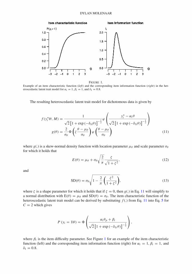
Figure 1.Example of an item characteristic function (left) and the corresponding item information function (right) in the het-eroscedastic latent trait model for αi = 1, βi = 1, and δ1 = 0.8.

The resulting heteroscedastic latent trait model for dichotomous data is given by

f (y∗i |θ, M) = 1

√2

[1 + exp (−δ1iθ)

]− 12

ϕ

⎛⎝ y∗

i − αiθ√

2[1 + exp (−δ1iθ)

]− 12

⎞⎠

g(θ) = 2

σθ

�

(ζ

θ − μθ

σθ

)ϕ

(θ − μθ

σθ

)(11)

where g(.) is a skew-normal density function with location parameter μθ and scale parameter σθ

for which it holds that

E(θ) = μθ + σθ

√2

π

ζ√1 + ζ 2

, (12)

and

SD(θ) = σθ

√1 − 2

π

(ζ 2

1 + ζ 2

), (13)

where ζ is a shape parameter for which it holds that if ζ = 0, then g(.) in Eq. 11 will simplify toa normal distribution with E(θ) = μθ and SD(θ) = σθ . The item characteristic function of theheteroscedastic latent trait model can be derived by substituting f (.) from Eq. 11 into Eq. 5 forC = 2 which gives

P (yi = 1|θ) = �

⎛⎝ αiθp + βi√

2[1 + exp (−δ1iθ)

]− 12

⎞⎠ ,

where βi is the item difficulty parameter. See Figure 1 for an example of the item characteristicfunction (left) and the corresponding item information function (right) for αi = 1, βi = 1, andδ1 = 0.8.

PSYCHOMETRIKA

1.4. Parameter Estimation and Implementation

The heteroscedastic latent trait models discussed in this paper can be fit to data using marginalmaximum likelihood estimation (MML; Bock & Aitkin, 1981). For the new model, an MMLestimation procedure is implemented in the statistical software package R (R Core Team, 2012).Specifically, −2 times the log of the marginal likelihood function (Eq. 1 with Eqs. 5 and 11)is minimized using the R built-in function ‘optim’. This optimizer uses a Broyden-Fletcher-Goldfarb-Shanno algorithm (BFGS; see e.g. Nocedal & Wright, 2006; p. 194) which is a quasi-Newton algorithm that uses first-order derivatives. The likelihood function is approximated using50 Gauss-Hermite quadrature points (see Molenaar et al., 2012). It is also possible to fit themodel using existing software like Mx (Neale, Aggen, Maes, Kubarych & Schmitt, 2006) andSAS (SAS Institute, 2011). The R scripts used here are available on the personal webpage of theauthor, together with an Mx script to fit the model.

2. Simulation Study

In this simulation study, the viability of the model for dichotomous data is investigated. Thatis, this simulation study is conducted to (1) investigate whether true parameters are adequatelyrecovered, (2) to assess what sample sizes are at least needed to apply the model, (3) to examinewhether δ1i and ζ can be disentangled satisfactorily, and (4) to see whether the statistical powerto detect the effects is acceptable given a reasonable effect size.

2.1. Design

Data are generated according to either (1) the full model with heteroscedastic residuals and askew-normal trait where both effects are in the same direction, denoted ‘het(+)’ and ‘skw(−)’ (i.e.a negatively skewed trait and increasing residuals for increasing trait levels); (2) the full modelwith heteroscedastic residuals and a skew-normal trait where both effects are in the oppositedirection, denoted ‘het(+)’ and ‘skw(+)’ (i.e. a positively skewed trait and increasing residualsfor increasing trait levels); (3) a model with het(+) only; and 4) a model with a skw(−) only.Sample sizes equalled 500, 1,000, 3,000 and 5,000; the number of items equalled 10 and 500replications were conducted for each condition. Parameter values in the case of item-specificheteroscedasticity effects (i.e. the effect of ‘het(+)’) are δ1i = 0.4 (‘small effect’), δ1i = 0.6(‘medium effect’), and δ1i = 0.8 (‘large effect’) for all i except for one item (δ1i = 0 for thisanchor item). For skw(+) and skw(−), ζ = 2.17 and ζ = −2.17 are used, respectively (‘mediumeffect’). The above effect sizes are based on Molenaar et al. (2010a, 2012).4 The anchor item wasthe 5th item. The remaining parameters were chosen to be αi = 1 for all i and the βi parameterswere chosen equally spaced in the interval [−1.5, 1.5]. In addition, E(θ) and SD(θ) were restrictedto equal 0 and 1 respectively.

2.2. Models and Power

Four models are fit to the generated datasets:

1. M0:2PM. A homoscedastic two-parameter model with a normal distribution for thetrait (i.e. a traditional two-parameter model (i.e. δ1i = 0 for all i and ζ = 0);

2. M1:het. A model with heteroscedastic residuals and a normal distribution for the trait(i.e. ζ = 0, and δ1i is free for all i except the anchor item);

4 Note that Molenaar et al. (2012) used δ0i = 1.5 instead of δ0i = 1,; therefore, in the present case, δ1i is rescaled tocorrespond to the effect size in Molenaar et al (i.e. due to the difference in δ0i , there is no one-to-one correspondence).

DYLAN MOLENAAR

3. M1:skw. A model with a skew-normal trait distribution and with homoscedastic residualvariances (i.e. ζ is free and δ1i = 0 for all i);

4. M2:full. A full model with both heteroscedastic residuals and a skewed trait (i.e. ζ isfree and δ1i is free for all i except the anchor item).

In all models, αi and βi are estimated for all i , and identification is accomplished by fixingE(θ) = 0, SD(θ) = 1, δ1i = 0 for the anchor item, and δ0i = 1, for all i .

For each model except M0:2PM (as this model serves as the baseline model), the powerof the likelihood ratio test to detect the effect(s) in the model is determined for a 0.05 levelof significance (e.g. Satorra & Saris, 1985). In the likelihood ratio test, HA is the model underconsideration (M1:het, M1:skw or M2:full) and H0 is the model without the effect of interest thatis nested in HA (i.e. M0:2PM, M1:het, or M1:skw). The likelihood ratio statistic is then given by

T = −2 × [ln L

(yp; τ̂ 0

) − ln L(yp; τ̂A

)],

where L(.) is given by Eq. 1, τ̂ 0 is the vector of parameter estimates of H0 and τ̂A is the vector ofparameter estimates of HA. As H0 is nested in HA, the parameter vector τ̂ 0 is a restricted versionof τ̂A. If the parameter constraints in H0 are not on the boundary of the parameter space, thenunder H0, T has a central χ2-distribution with degrees of freedom (df) equal to the number ofrestrictions in H0. Under HA, T has a non-central χ2-distribution with non-centrality parameterλ and with df equal to the number of restrictions in H0. To calculate power, the non-centralityparameter needs to be estimated. As it holds that E(T) = d f +λ (see Fisher, 1928), an estimate ofλ could be obtained by averaging T -df over the replications in the simulation study. Next, poweris obtained by integrating the non-central χ2 distribution from the critical value to ∞.

3. Results

3.1. Parameter Recovery and Sample Size

In Table 2, results are depicted for the conditions in which the true model includes het-eroscedastic residuals with a small effect size. Items are sorted according to their item difficultyparameter, where item 1 is located at the lower θ range and item 10 is located at the upper θ range.As can be seen, for N = 5, 000 and N = 3, 000, parameters are acceptably recovered. For item10, variability is large due to, respectively, 1 and 9 diverged estimates in the case of N = 5, 000and N = 3, 000. For N = 1, 000 and N = 500, estimates of δ1i are diverging in an increasingnumber of cases causing large parameter variability for the items at the upper and lower end ofthe θ range. See Figure 2 for a histogram of the parameter estimates of δ1i for item 10 (an itemat the upper range of θ) for N = 1, 000 and N = 500. As can be seen, the estimates centreapproximately around the true value (0.4), but a number of estimates diverged. Apparently, forthe cases that diverged, there was not enough information in the data concerning the δ1i parameter.

Results for the model with a skewed latent trait only (δ1i = 0 and ζ = −2.17) are nottabulated but were generally good. Specifically, parameter estimates (SD) for ζ in this conditionare −2.19(0.30),−2.22(0.39),−2.27(0.81) and −2.54(1.48) for samples sizes of, respectively,5,000, 3,000, 1,000 and 500. From these results and the results concerning ζ in Table 2, it couldbe concluded that the true value is well recovered for all sample sizes. Notably, in the case ofN = 500, the parameter estimate variability tends to be quite large.

3.2. Power and Resolvability

Table 3 depicts the power to detect heteroscedasticity in the items (i.e. the power to detectthat δ1i �= 0) for a model with heteroscedastic residuals only (M1:het) and a model with both

PSYCHOMETRIKA

Ta

ble

2.M

ean

(sta

ndar

dde

viat

ion)

ofth

ees

timat

esfo

rδ 1

ian

dζ

inth

eco

rrec

tmod

elfo

rea

chco

nditi

onin

the

case

ofa

smal

leff

ects

ize.

Tru

eva

lues

i=1

i=2

i=3

i=4

i=6

i=7

i=8

i=9

i=10

δ 1i

ζ

δ 1i=

0.4;

ζ=

0N

=5,

000

0.42

(0.2

2)0.

39(0

.21)

0.39

(0.2

0)0.

40(0

.21)

0.42

(0.2

2)0.

41(0

.25)

0.45

(0.2

8)0.

46(0

.35)

0.50

(0.5

1)–

N=

3,00

00.

39(0

.30)

0.41

(0.2

7)0.

41(0

.27)

0.41

(0.2

6)0.

41(0

.29)

0.44

(0.3

7)0.

46(0

.44)

0.48

(0.4

6)0.

80(3

.04)

–N

=1,

000

0.07

(3.2

1)0.

41(0

.60)

0.40

(0.5

4)0.

46(0

.57)

0.46

(0.6

6)0.

54(0

.71)

0.61

(1.0

3)0.

98(3

.53)

1.93

(6.4

5)–

N=

500

−1.3

6(8

.81)

0.08

(3.0

9)0.

40(1

.19)

0.47

(0.9

7)0.

63(2

.65)

1.06

(3.2

2)1.

46(4

.78)

2.47

(7.5

1)4.

59(1

1.01

)–

δ 1i=

0.4;

ζ=-

2.17

N=

5,00

00.

41(0

.22)

0.43

(0.2

2)0.

43(0

.25)

0.43

(0.2

5)0.

44(0

.31)

0.43

(0.3

6)0.

43(0

.38)

0.45

(0.4

5)0.

58(2

.12)

−2.2

2(0

.90)

N=

3,00

00.

41(0

.30)

0.44

(0.3

0)0.

45(0

.31)

0.43

(0.3

3)0.

47(0

.41)

0.44

(0.4

5)0.

46(0

.51)

0.64

(2.4

9)1.

21(4

.98)

−2.2

9(1

.14)

N=

1,00

00.

22(3

.02)

0.47

(0.7

2)0.

46(0

.59)

0.45

(0.6

0)0.

65(1

.19)

0.56

(0.9

9)0.

71(2

.86)

2.24

(7.9

7)3.

68(1

0.98

)−2

.44

(1.9

7)N

=50

0−0

.54

(6.1

9)0.

28(3

.87)

0.60

(1.3

1)0.

81(2

.78)

1.11

(3.6

2)1.

31(4

.93)

3.06

(9.4

8)5.

01(1

2.84

)7.

57(1

5.34

)−2

.53

(2.5

7)δ 1

i=

0.4;

ζ=

2.17

N=

5,00

00.

39(0

.37)

0.42

(0.3

5)0.

44(0

.36)

0.44

(0.3

4)0.

45(0

.30)

0.41

(0.3

0)0.

40(0

.30)

0.41

(0.3

4)0.

50(1

.53)

2.25

(0.9

5)N

=3,

000

0.44

(0.4

6)0.

42(0

.42)

0.46

(0.4

7)0.

45(0

.46)

0.44

(0.3

9)0.

42(0

.39)

0.43

(0.3

5)0.

43(0

.43)

0.55

(2.0

2)2.

30(1

.20)

N=

1,00

0−0

.06

(3.8

4)0.

40(1

.29)

0.42

(0.8

5)0.

47(0

.80)

0.45

(0.6

6)0.

52(0

.76)

0.64

(2.0

0)1.

11(4

.37)

2.37

(8.0

6)2.

31(1

.49)

N=

500

−2.5

6(1

0.59

)−0

.12

(5.0

3)0.

26(3

.77)

0.80

(2.6

9)0.

44(2

.60)

0.90

(3.8

8)1.

75(6

.67)

3.76

(10.

58)

6.29

(14.

19)

2.54

(1.7

1)

δ 1i

isfix

edto

0fo

ri

=5

(anc

hor

item

).It

ems

are

sort

edac

cord

ing

toth

eir

item

diffi

culty

.For

the

resu

ltsco

ncer

ning

the

cond

ition

with

ask

ewed

late

nttr

aito

nly,

see

text

.

DYLAN MOLENAAR

Figure 2.Histograms of the heteroscedasticity parameter estimates for item 10 across replications. The true value equals 0.4.

Table 3.Power of a model with heteroscedastic residuals only (M1:het) and the full model (M2:full) to detect heteroscedasticityin the items for a 0.05 level of significance.

Condition N Small effect Medium effect Large effect

M1:het M2:full M1:het M2:full M1:het M2:full

het(+) & skew(−) 5,000 1.00 (126.15) 0.60 (10.70) 1.00(191.71) 0.98 (27.94) 1.00 (264.19) 1.00 (53.63)3,000 1.00 (76.43) 0.35 (6.13) 1.00 (116.03) 0.86 (17.89) 1.00 (157.33) 0.99 (31.67)1,000 0.96 (24.58) 0.12 (1.77) 1.00 (38.29) 0.34 (5.95) 1.00 (53.36) 0.61 (10.83)500 0.71 (13.14) 0.07 (0.69) 0.89 (19.32) 0.16 (2.84) 0.97 (26.57) 0.19 (3.37)

het(+) 5,000 1.00 (35.25) 0.22 (3.88) 1.00 (74.30) 0.59 (10.53) 1.00 (124.41) 0.94 (22.92)3,000 0.92 (20.74) 0.12 (1.88) 1.00 (45.18) 0.35 (6.24) 1.00 (75.33) 0.75 (14.09)1,000 0.40 (7.09) 0.07 (0.69) 0.76 (14.33) 0.13 (2.03) 0.96 (25.34) 0.26 (4.62)500 0.25 (4.42) 0.07 (0.65) 0.46 (8.16) 0.09 (1.19) 0.70 (12.84) 0.15 (2.55)

skew(−) 5,000 0.99 (30.84) 0.05 (0.14) 0.99 (30.84) 0.05(0.14) 0.99 (30.99) 0.05 (0.04)3,000 0.88 (18.86) 0.05 (0.07) 0.89 (19.04) 0.06 (0.29) 0.87 (18.44) 0.06 (0.18)1,000 0.38 (6.78) 0.06 (0.39) 0.37 (6.59) 0.05 (0.00) 0.40 (6.98) 0.05 (0.02)500 0.21 (3.77) – 0.21 (3.79) – 0.24 (4.20) 0.06 (0.32)

het(+) & skew(+) 5000 0.06 (0.27) 0.25 (4.49) 0.51 (9.08) 0.52 (9.19) 0.98 (29.00) 0.77 (14.85)3,000 0.05 (0.03) 0.15 (2.45) 0.26 (4.60) 0.29 (5.17) 0.82 (16.29) 0.47 (8.28)1,000 0.07 (0.47) 0.07 (0.50) 0.13 (2.04) 0.11 (1.64) 0.35 (6.13) 0.10 (1.38)500 0.09 (1.09) – 0.11 (1.62) – 0.21 (3.69) –

het(+): heteroscedastic residuals that increase for increasing levels of θ ; skw(−): negatively skewed trait;skw(+): positively skewed trait. ‘−‘: in these cases, the non-centrality parameter was slightly negative dueto a too small sample size.

heteroscedastic residuals and a skew-normal trait (M2:full). First, it can be seen from the tablethat in the case of the ‘het(+) & skew(−)’ condition, the pattern of results is generally acceptable.That is, for increasing sample sizes and increasing effect sizes, power coefficients approach atleast a 0.80 level. In the case of the ‘het(+)’ condition, the M1:het model has acceptable powerto detect the effect for increasing effect size and sample size, while the M2:full model has onlyacceptable power for a large effect. Apparently, incorporation of the additional shape parameter ζ ,while the effect is actually not in the data, results in a decrease in power. An interesting conditionis the case that there is a skewed trait in the data only (i.e. the ‘skew(+)’ condition), as conclusionsconcerning resolvability of the effects could be inferred from the results in this condition. As canbe seen, the skewed trait effect is absorbed in the heteroscedasticity parameters δ1i in the M1:het

PSYCHOMETRIKA

model (i.e. the power is large). Thus, unmodelled skewness in the trait will incorrectly be detectedas heteroscedasticity (i.e. false positives). However, in the full model M2:full, where the skewnessin the trait is accounted for by introducing the ζ parameter, the power to detect heteroscedasticityadequately equals the Type I error rate (0.05). This indicates that the effect of skewness in thetrait is well separable from heteroscedastic residuals. Finally, it can be seen from the table that inthe ‘het(+) & skw(+)’ condition, the effects may cancel out depending on the effect size. That is,for the small and medium heteroscedasticity effect size, power is much smaller as compared tothe ‘het(+) & skew(−)’ condition. For the large effect size and N = 5, 000, power is acceptableagain.

4. Conclusion

From the simulation study, it appears that parameter recovery is generally acceptable. How-ever, in smaller sample sizes, estimates for the heteroscedasticity parameter δ1i are much morelikely to diverge from the population value for items that have difficulty parameters at the extremesof the trait. The power results indicated that by the identification constraint δ1i = 0 for the anchoritem, the effects on the trait distribution and the residual variances are resolvable. That is, one candistinguish between a common effect of heteroscedasticity (formalized as a skewed trait) and/oritem-specific effects (operationalized as heteroscedastic residual variances), given that the effectsare not in the same direction. In the case that the effects are in the same direction (e.g. a positivelyskewed trait and increasing residual variance across the trait), they may cancel each other outdepending on the effect size. With respect to the sample size needed to apply the model, it couldbe concluded that relatively large sample sizes are needed. Power is only acceptable for samplesizes of at least 1,000 subjects when a single effect is considered, or sample sizes of at least 3,000subjects when both effects are combined. This will be further discussed in the final section.

While the simulation study shows that the anchor item is useful to distinguish item commoneffects and item-specific effects of heteroscedasticity, the question arises of how an anchor itemshould be identified. In application 2 below, the use of Lagrange Multipliers (LM) is illustrated.The multivariate LM statistic signifies the approximate increase in loglikelihood that will resultfrom freeing each constraint parameter. This statistic can be calculated by G′

0H0G0, where G0 isthe vector of first-order derivatives of the loglikelihood function and H0 is the matrix of second-order derivatives to the model parameters in the baseline model. Using this formula, univariateLM statistics could be calculated for each constrained parameter separately. As will be shown inapplication 2, univariate LM statistics can be calculated for the δ1i parameter of each item in amodel with a skewed trait. Then, these LM statistics will indicate whether —after taking the traitskewness into account—it is beneficial to incorporate additional item-specific heteroscedasticityeffects. In the present paper, LM statistics are obtained by the exact first-order derivatives, G0.The second-order derivatives in H0 are obtained by a finite difference approximation. Simulationsshowed that this works well (see also Dolan & Molenaar, 1991).

5. Illustrations

5.1. Illustration 1: Alcohol Use

The data comprises scores of 4,627 subjects on 5 items of the Michigan Alcohol ScreeningTest (Selzer, 1971) which was administered in the National Survey of Midlife Development in theUnited States (MIDUS) in 1995–1996 under the auspices of the Inter-university Consortium for

DYLAN MOLENAAR

Table 4.Model fit results for application 1.

−2LL LRT d f AIC BIC sBIC DIC

1. Baseline 6,370.02 6,390 6,454 6,423 6,4362. Heteroscedastic residuals 6,363.39 6.63 5 6,393 6,490 6,442 6,4623. Skew trait distribution 6,354.51 8.88 1 6,377 6,447 6,412 6,427

−2LL denotes −2 times the loglikelihood. The likelihood ratio test (LRT) is conducted between the corre-sponding model and the baseline model. For the fit indices, the best values are in boldface.

Political and Social Research (ICPSR), see (Grzywacz & Marks, 1999).5 The items are yes/noquestions about possible consequences of alcohol use, for instance

‘Did you ever, during the past 12 months, have any emotional or psychological prob-lems from using alcohol – such as feeling depressed, being suspicious of people, orhaving strange ideas?’

Unidimensionality of the data was assessed to ensure that possible heteroscedasticity effectsare not due to misfit (e.g. multidimensionality). Using Mplus (Muthén & Muthén, 2007), a two-parameter probit model was fit to the tetrachoric correlation matrix using weighted least-squaresestimation. The model fit was considered good according to the RMSEA which equals 0.03, theCFI which equals 0.993, and the TLI which equals 0.986.6

6. Results

Different models were fit to investigate whether heteroscedastic residuals and/or a skewedtrait distribution underlie the data. See Table 4 for the results. First, a model with homoscedasticresiduals and a normal trait distribution was considered. This model is a traditional two-parametermodel and served as a baseline model. Then, all heteroscedasticity parameters δ1i were freedresulting in a model with heteroscedastic residual variances in all items. As indicated by thelikelihood ratio test, AIC, BIC, sBIC, and DIC, the fit of this model was not an improvement overthe baseline model, that is, the restriction δ1i = 0 were tenable. Next, a model with a skew-normaltrait distribution was fit to test whether a general effect can be detected that is not picked up bythe individual items. According to the fit indices, this model was the best-fitting model. As canbe seen from the table, the estimate of ζ equals 2.739, see Figure 3 for the implied distributionof θ . As can be seen from the figure and the parameter estimate, the alcohol use trait is positivelyskewed, indicating that more subjects are relatively unproblematic alcohol users. This is in linewith the Lucke’s (2012) argument that a normal distribution for traits like addiction is theoreticallysuboptimal. An even better theoretically motivated distribution might be a distribution with support[0,∞), see Lucke (2012).

6.1. Illustration 2: Scores on the Raven test

The data consist of the responses of 2,301 first-year psychology students to the Raven’sProgressive Matrices (Raven, 2000) collected between 2001 and 2009 at the University of Ams-terdam (Bakker & Wicherts, 2013; see also Wicherts & Bakker, 2012). From the 36 items, 10

5 The opinions expressed in this article are those of the author and do not necessarily reflect the views of the ICPSR.6 RMSEA values smaller than 0.05 are generally considered to indicate good model fit. CFI and TLI values larger

than 0.95 are considered to indicate good model fit, see Hu and Bentler (1999)

PSYCHOMETRIKA

Figure 3.Solid line The estimated distribution of the alcohol trait in application 1. Dashed line a normal distribution as specifiedunder the baseline model.

items were selected. Proportions correct of these items are 0.82, 0.71, 0.70, 0.71, 0.65, 0.70, 0.55,0.59, 0.36 and 0.48. Models were again fit in R as described in application 1. As before, to assessunidimensionality, a one factor model was fit to the data. Results indicated that unidimensionalityis tenable as judged by the RMSEA (0.040), the CFI (0.952) and the TLI (0.957).

7. Results

First, a traditional two-parameter model and a model with heteroscedastic residuals only werefit. See Table 5 for the modelling results. As can be seen, it was unclear whether the model withheteroscedastic residuals (model 2) is an improvement over the baseline model (model 1). Thatis, the LRT, AIC and sBIC indicate that model 2 is the better fitting model, while the BIC and DICindicate that model 1 is the better fitting model. However, the large likelihood ratio might indicatethat at least some items are associated with heteroscedastic residuals. This was studied next. First,a model with a skewed trait distribution was fit (model 3a). All fit indices indicated that this modelfits better than the traditional model. As the likelihood ratio already indicated that heteroscedasticresiduals characterize these data, the question arose whether this heteroscedasticity is due to theskewed trait, or whether some additional item-specific heteroscedasticity is present. To investigatethis question, univariate LM statistics were calculated within model 3a for the δ1i parameters ofall items as discussed above.

The univariate LM statistics for δ1i equaled 1.05, 0.17, 16.14, 13.07, 6.52, 8.51, 0.48, 28.01,0.71 and 0.22 for items 1–10, respectively. As these statistics are χ2(1) distributed, δ1i was freedfor items 3, 4, 5, 6 and 8. In the resulting model 3b, Lagrange multipliers for the fixed δ1i equaled,respectively, 0.11, 1.73, 1.73, 0.01 and 2.98 for item 1, 2, 7, 9 and 10. That is, there was noindication of additional item-specific heteroscedasticity. As can be seen in Table 5, the LRT, AICand sBIC indicate that this model fits best among the models considered. The BIC favours the

Table 5.Model fit results for application 2.

Model −2LL LRT d f AIC BIC sBIC DIC

1. Baseline 26,854.90 26,895 27,010 26,946 26,9732. Heteroscedastic residuals 26,801.26 2 vs. 1: 53.64 10 26,861 27,034 26,938 26,9783a. Skew trait distribution 26,835.15 3 vs. 1: 19.75 1 26,877 26,998 26,931 26,9593b. Skew and het. on 3,4,5,6, 8 26,805.48 3b vs. 3a: 29.67 5 26,857 27,007 26,924 26,959

−2LL denotes −2 times the loglikelihood. For the fit indices, best values are in boldface.

DYLAN MOLENAAR

Table 6.Parameter estimates for the final model (model 3b) in application 2.

Item no Baseline Model 3b

αi βi αi βi δ1i

1 0.509 1.037 0.492 1.029 –2 0.370 0.584 0.367 0.582 –3 0.468 0.581 0.484 0.635 0.7974 0.591 0.642 0.593 0.713 1.0465 0.423 0.430 0.427 0.484 0.7736 0.633 0.619 0.633 0.678 0.7517 0.915 0.179 0.926 0.164 –8 1.158 0.337 1.001 0.009 −3.6519 0.670 −0.437 0.668 −0.443 –10 0.700 −0.062 0.693 −0.071 –ζ − −1.570

model without item-specific heteroscedasticity, and the DIC is undecided. As most indices favourmodel 3b, this model was accepted as the final model. See Table 6 for the parameter estimatesin this model and the parameter estimates in the baseline model (model 1, i.e. a traditional two-parameter model). The item characteristic functions of items 3, 4, 5, 6 and 8 that are associatedwith item-specific heteroscedasticity are in Figure 4 both under the homoscedastic model (stripedline) and under the heteroscedastic model (solid line). The item information functions for theseitems are in Figure 5 again both under the homoscedastic model (dashed line) and under theheteroscedastic model (solid line). As can be seen from Figure 4, the item characteristic functionin the homoscedastic case approximates the function in the heteroscedastic case, with systematicunder- or over-prediction. Most importantly, as the heteroscedastic ICFs are asymmetric, the pointat which the slope of the ICF has it maximum can differ noticeably between the homoscedasticand heteroscedastic cases. This causes the estimated amount of item information and the locationon the θ -scale at which the maximum amount of information is obtained to differ considerablybetween the homoscedastic and heteroscedastic models, as can be seen from Figure 5.

8. Discussion

From the results in this paper, it can be concluded that disentangling heteroscedastic residualsfrom skewness in the latent trait is a possible but demanding endeavour. As dichotomous datacontain less information concerning individual differences, larger sample sizes were needed ascompared to the polytomous case. In the polytomous case, Molenaar et al. (2012) obtained sat-isfactory modelling results (acceptable power and parameter recovery) for N = 400, while in thepresent paper, at least 1,000 to 3,000 subjects were needed. Therefore, the model seems most use-ful in cases where large sample sizes are involved (e.g. computerized adaptive testing or nationalsurveys). That is, in these cases, effects of heteroscedasticity could be discovered. However, forsmaller sample sizes, it could be sufficient to only consider a skew-normal distribution for thetrait, as from the simulation study and the applications, it appears that most of the effects ofheteroscedasticity could be captured in this way.

In the present paper, a distinction was made between latent and observed moderators. Inthe case of an observed moderator, the moderator is external to the measurement model (i.e. the

PSYCHOMETRIKA

Figure 4.Solid line The model implied item characteristic functions for the items that display heteroscedasticity in application 2.Dashed line the item characteristic functions for the corresponding item under the baseline model (a traditional two-parameter model).

moderator is not an indicator from the measurement model). In the case of a latent moderatorvariable, it was assumed that the moderator is latent to the data at hand. An interesting possibility toconsider in future research is the case in which the latent moderator will be an external latent traitwith its own measurement model. This will address the latent variable interaction literature (Kenny& Judd, 1984; Klein & Moosbrugger, 2000). The models could be interesting in for instance testingthe personality differentiation hypothesis (Austin, Deary, & Gibson, 1997), which postulates thatpersonality and intelligence interact. In addition, in the field of behaviour genetics, genotypeby environment interactions are investigated by either the latent continuous moderator approach(Molenaar, van der Sluis, Boomsma, & Dolan, 2012; Van der Sluis et al., 2006) or the observedcontinuous moderator approach (Purcell, 2002; van der Sluis et al., 2012). For instance, it was

DYLAN MOLENAAR

Figure 5.Solid line The model implied item information functions for items that display heteroscedasticity in application 2. Dashedline the item information function for the corresponding item under the baseline model (a traditional two-parametermodel). The x-scales of the plots are deliberately chosen to be the same as in Figure 5.

found that for cognitive ability tests, the genetic factor is heteroscedastic across socioeconomicstatus (Turkheimer, Haley, Waldron, D’Onofrio, & Gottesman, 2003) indicating a genotype byenvironment interaction on cognitive ability. If heteroscedasticity of the genetic factor across alatent trait is of interest (e.g. depression), then an external latent moderator approach might beuseful.

Acknowledgments

In memory of Roger Millsap whose comments and guidance were of great help in preparingthe final version of this paper. I am also indebted to Mijke Rhemtulla, Conor Dolan, and twoanonymous reviewers for their valuable comments on a previous draft of the manuscript.

PSYCHOMETRIKA

References

Anderson, M. J. (2006). Distance-based tests for homogeneity of multivariate dispersions. Biometrics, 62, 245–253.Andrich, D. (1978). A rating formulation for ordered response categories. Psychometrika, 43, 561–573.Austin, E. J., Deary, I. J., & Gibson, G. J. (1997). Relationships between ability and personality: Three hypotheses tested.

Intelligence, 25(1), 49–70.Azevedo, C. L. N., Bolfarine, H., & Andrade, D. F. (2011). Bayesian inference for a skew-normal IRT model under the

centred parameterization. Computational Statistics & Data Analysis, 55, 353–365.Azzalini, A. (1985). A class of distributions which includes the normal ones. Scandinavian Journal of Statistics, 12,

171–178.Azzalini, A. (1986). Further results on a class of distributions which includes the normal ones. Statistica, 46, 199–208.Azzalini, A., & Capatanio, A. (1999). Statistical applications of the multivariate skew normal distribution. Journal of the

Royal Statistical Society, Series B, 61, 579–602.Bakker, M., & Wicherts, J. M. (2013). Outlier removal, sum scores, and the inflation of the type I error rate in independent

samples t tests: The power of alternatives and recommendations. Psychological Methods. doi:10.1037/met0000014.Bartholomew, D. J., Knott, M., & Moustaki, I. (2011). Latent variable models and factor analysis: A unified approach.

UK: Wiley.Bauer, D. J., & Hussong, A. M. (2009). Psychometric approaches for developing commensurate measures across inde-

pendent studies: Traditional and new models. Psychological Methods, 14(2), 101–125.Bazán, J. L., Branco, M. D., & Bolfarine, H. (2006). A skew item response model. Bayesian Analysis, 1, 861–892.Birnbaum, A. (1968). Some latent trait models and their use in inferring an examinee’s ability. In E. M. Lord & M. R.

Novick (Eds.), Statistical theories of mental test scores (chap (pp. 17–20). Reading, MA: Addison Wesley.Bock, R. D. (1972). Estimating item parameters and latent ability when responses are scored in two or more nominal

categories. Psychometrika, 37, 29–51.Bock, R. D., & Aitkin, M. (1981). Marginal maximum likelihood estimation of item parameters: Application of an EM

algorithm. Psychometrika, 46, 443–459.Bollen, K. A. (1989). Structural equations with latent variables. New York: Wiley.Bollen, K. A. (1996). A limited-information estimator for LISREL models with or without heteroscedastic errors. In

G. A. Marcoulides & R. E. Schumacker (Eds.), Advanced structural equation modeling: Issues and techniques (pp.227–241). Mahwah, NJ: Erlbaum.

Brunner, E., Dette, H., & Munk, A. (1997). Box-Type Approximations in Nonparametric Factorial Designs. Journal ofthe American Statistical Association, 92, 1494–1502.

Christoffersson, A. (1975). Factor analysis of dichotomized variables. Psychometrika, 40, 5–32.Dobson, A. J. (2010). An introduction to generalized linear models. Boca Raton, FL: CRC Press.Dolan, C. V. (1994). Factor analysis of variables with 2, 3, 5 and 7 response categories: A comparison of categorical variable

estimators using simulated data. British Journal of Mathematical and Statistical Psychology, 47(2), 309–326.Dolan, C. V., Colom, R., Abad, F. J., Wicherts, J. M., Hessen, D. J., & van de Sluis, S. (2006). Multi-group covariance

and mean structure modeling of the relationship between the WAIS-III common factors and sex and educationalattainment in Spain. Intelligence, 34, 193–210.

Dolan, C. V., & van der Maas, H. L. (1998). Fitting multivariage normal finite mixtures subject to structural equationmodeling. Psychometrika, 63, 227–253.

Dolan, C. V., & Molenaar, P. (1991). A comparison of four methods of calculating standard errors of maximum-likelihoodestimates in the analysis of covariance structure. British Journal of Mathematical and Statistical Psychology, 44,359–368.

Fisher, R.A. (1928). The general sampling distribution of the multiple correlation coefficient. Proceedings of the RoyalSociety of London. Series A, 121, 654–673.

Fischer, G. H. (1983). Logistic latent trait models with linear constraints. Psychometrika, 48, 3–26.Fokkema, M., Smits, N., Kelderman, H., & Cuijpers, P. (2013). Response shifts in mental health interventions: An

illustration of longitudinal measurement invariance. Psychological Assessment, 25, 520–531.Greene, W. (2011). Econometric analysis (7th ed.). New York: Prentice Hall.Grzywacz, J. G., & Marks, N. F. (1999). Family solidarity and health behaviors: Evidence from the National Survey of

Midlife Development in the United States. Journal of Family Issues, 20(2), 243–268.Harvey, A.C. (1976). Estimating regression models with multiplicative heteroscedasticity. Econometrica: Journal of the

Econometric Society, 44, 461–465.Hessen, D. J., & Dolan, C. V. (2009). Heteroscedastic one-factor models and marginal maximum likelihood estimation.

British Journal of Mathematical and Statistical Psychology, 62, 57–77.Hu, L. T., & Bentler, P. M. (1999). Cutoff criteria for fit indexes in covariance structure analysis: Conventional criteria

versus new alternatives. Structural Equation Modeling: A Multidisciplinary Journal, 6(1), 1–55.Jansen, B. R., & van der Maas, H. L. (1997). Statistical test of the rule assessment methodology by latent class analysis.

Developmental Review, 17, 321–357.Jarque, C. M., & Bera, A. K. (1980). Efficient tests for normality, homoscedasticity and serial independence of regression

residuals. Economics Letters, 6, 255–259.Jedidi, K., Jagpal, H. S., & DeSarbo, W. S. (1997). Finite mixture structural equation models for response based segmen-

tation and unobserved heterogeneity. Marketing Science, 16, 39–59.Jöreskog, K. G. (1971). Simultaneous factor analysis in several populations. Psychometrika, 36, 409–426.

DYLAN MOLENAAR

Jöreskog, K. G., & Moustaki, I. (2001). Factor analysis of ordinal variables: A comparison of three approaches. MultivariateBehavioral Research, 36, 347–387.

Kenny, D. A., & Judd, C. M. (1984). Estimating the nonlinear and interactive effects of latent variables. PsychologicalBulletin, 96, 201–210.

Kirisci, L., Hsu, T., & Yu, L. (2001). Robustness of item parameter estimation programs to assumptions of unidimension-ality and normality. Applied Psychological Measurement, 25, 146–162.

Klein, A., & Moosbrugger, H. (2000). Maximum likelihood estimation of latent interaction effects with the LMS method.Psychometrika, 65, 457–474.

Lee, S. Y., Poon, W. Y., & Bentler, P. M. (1989). Simultaneous analysis of multivariate polytomous variates in severalgroups. Psychometrika, 54, 63–73.

Lewin-Koh, S., & Amemiya, Y. (2003). Heteroscedastic factor analysis. Biometrika, 90, 85–97.Long, J. S., & Ervin, L. H. (2000). Using heteroscedasticity consistent standard errors in the linear regression model. The

American Statistician, 54, 217–224.Lord, F. M. (1952). A theory of test scores. New York: Psychometric Society.Lucke, J.F. (2012). Positive Trait Item Response Models. Proceedings of the 2012 Joint Statistical Meetings of the

American Statistical Association, the International Biometric Society, the Institute of Mathematical Statistics, andStatistica Canada. San Diego, CA. 2012. Retrieved from http://works.bepress.com/joseph_lucke/35

Masters, G. N. (1982). A Rasch model for partial credit scoring. Psychometrika, 47, 149–174.Mehta, P. D., & Neale, M. C. (2005). People are variables too: Multilevel structural equations modeling. Psychological

Methods, 10, 259–284.Mehta, P. D., Neale, M. C., & Flay, B. R. (2004). Squeezing interval change from ordinal panel data: Latent growth curves

with ordinal outcomes. Psychological Methods, 9, 301.Meijer, E., & Mooijaart, A. (1996). Factor analysis with heteroscedastic errors. British Journal of Mathematical and

Statistical Psychology, 49, 189–202.Merkle, E. C., Fan, J., & Zeileis, A. (2013). Testing for measurement invariance with respect to an ordinal variable.

Psychometrika, 1–16. doi:10.1007/s11336-013-9376-7.Merkle, E. C., & Zeileis, A. (2013). Tests of measurement invariance without subgroups: A generalization of classical

methods. Psychometrika, 78, 59–82.Mellenbergh, G. J. (1994a). A unidimensional latent trait model for continuous item responses. Multivariate Behavioral

Research, 29, 223–236.Mellenbergh, G. J. (1994b). Generalized linear item response theory. Psychological Bulletin, 115, 300–307.Meredith, W. (1993). Measurement invariance, factor analysis and factorial invariance. Psychometrika, 58, 525–543.Millsap, R. E., & Yun-Tein, J. (2004). Assessing factorial invariance in ordered-categorical measures. Multivariate Behav-

ioral Research, 39, 479–515.Mislevy, R. J., & Verhelst, N. (1990). Modeling item responses when different subjects employ different solution strategies.

Psychometrika, 55, 195–215.Molenaar, D., Dolan, C. V., & de Boeck, P. (2012a). The heteroscedastic graded response model with a skewed latent

trait: Testing statistical and substantive hypotheses related to skewed item category functions. Psychometrika, 77,455–478.

Molenaar, D., Dolan, C. V., & van der Maas, H. L. (2011). Modeling ability differentiation in the second order factormodel. Structural Equation Modeling, 18, 578–594.

Molenaar, D., Dolan, C. V., & Verhelst, N. D. (2010a). Testing and modeling non-normality within the one factor model.British Journal of Mathematical and Statistical Psychology, 63, 293–317.

Molenaar, D., van der Sluis, S., Boomsma, D. I., & Dolan, C. V. (2012b). Detecting specific genotype by environmentinteraction using marginal maximum likelihood estimation in the classical twin design. Behavior Genetics, 42, 483–499.

Molenaar, D., Dolan, C. V., Wicherts, J. M., & van der Maas, H. L. J. (2010b). Modeling differentiation of cognitiveabilities within the higher-order factor model using moderated factor analysis. Intelligence, 38, 611–624.

Moustaki, I., & Knott, M. (2000). Generalized latent trait models. Psychometrika, 65, 391–411.Murray, A. L., Dixon, H., & Johnson, W. (2013). Spearman’s law of diminishing returns: A statistical artifact? Intelligence,

41, 439–451.Muthén, B. O. (1978). Contributions to factor analysis of dichotomous variables. Psychometrika, 43, 551–560.Muthén, B. O., & Christoffersson, A. (1981). Simultaneous factor analysis of dichotomous variables in several groups.

Psychometrika, 46, 407–419.Muthén, L. K., & Muthén, B. O. (2007). Mplus user’s guide (5th edn.). Los Angeles, CA: Muthén & Muthén.Neale, M. C., Aggen, S. H., Maes, H. H., Kubarych, T. S., & Schmitt, J. E. (2006a). Methodological issues in the assessment

of substance use phenotypes. Addicitive Behavior, 31, 1010–34.Neale, M. C., Boker, S. M., Xie, G., & Maes, H. H. (2006b). Mx: Statistical modeling (7th ed.). VCU, Richmond, VA:

Author.Nocedal, J., & Wright, S. J. (2006). Numerical optimization (2nd ed.). New York: Springer.Olsson, U. (1979). Maximum likelihood estimation of the polychoric correlation coefficient. Psychometrika, 44, 443–460.Purcell, S. (2002). Variance components models for gene-environment interaction in twin analysis. Twin Research, 5,

554–571.Rabe-Hesketh, S., Skrondal, A., & Pickles, A. (2004). Generalized multilevel structural equation modeling. Psychometrika,

69, 167–190.

PSYCHOMETRIKA

R Core Team. (2012). R: A language and environment for statistical computing. Vienna, Austria: R Foundation forStatistical Computing.

Raven, J. (2000). The Raven’s progressive matrices: Change and stability over culture and time. Cognitive Psychology,41, 1–48.

Ree, M. J. (1979). Estimating item characteristic curves. Applied Psychological Measurement, 3, 371–385.Rost, J. (1990). Rasch models in latent classes: An integration of two approaches to item analysis. Applied Psychological

Measurement, 14, 271–282.Samejima, F. (1969). Estimation of ability using a response pattern of graded scores (Psychometric Monograph No. 17).

Richmond, VA: The Psychometric Society.Samejima, F. (1997). Departure from normal assumptions: A promise for future psychometrics with substantive mathe-

matical modeling. Psychometrika, 62, 471–493.Samejima, F. (2000). Logistic positive exponent family of models: Virtue of asymmetric item characteristic curves.

Psychometrika, 65, 319–335.Samejima, F. (2008). Graded response model based on the logistic positive exponent family of models for dichotomous

responses. Psychometrika, 73, 561–578.SAS Institute. (2011). SAS/STAT 9.3 user’s guide. SAS Institute.Satorra, A., & Saris, W. E. (1985). The power of the likelihood ratio test in covariance structure analysis. Psychometrika,

50, 83–90.Selzer, M. L. (1971). The michigan alcohol screening test: The quest for a new diagnostic instrument. American Journal

of Psychiatry, 127, 89–94.Seong, T. J. (1990). Sensitivity of marginal maximum likelihood estimation of item and ability parameters to the charac-

teristics of the prior ability distributions. Applied Psychological Measurement, 14, 299–311.Skrondal, A. (1996). Latent trait, multilevel and repeated measurement modeling with incomplete data of mixed measure-

ment levels. Oslo: UiO .Skrondal, A., & Rabe-Hesketh, S. (2004). Generalized latent variable modeling: Multilevel, longitudinal, and structural

equation models. Boca Raton, FL: Chapman and Hall/CRC.Slutsky, E. E. (1913). On the criterion of goodness of fit of the regression lines and on the best method of fitting them to

the data. Journal of the Royal Statistical Society, 77, 78–84.Stevens, J. (2009). Applied multivariate statistics for the social sciences. USA: Taylor & Francis.Stone, C. A. (1992). Recovery of marginal maximum likelihood estimates in the two-parameter logistic response model:

An evaluation of MULTILOG. Applied Psychological Measurement, 16, 1–16.Swaminathan, H., & Gifford, J. (1983). Estimation of parameters in the three- parameter latent trait model. In D. J. Weiss

(Ed.), New horizons in testing: Latent trait test theory and computerized adaptive testing (pp. 13–30). New York:Academic Press.

Takane, Y., & de Leeuw, J. (1987). On the relationship between item response theory and factor analysis of discretizedvariables. Psychometrika, 52, 393–408.

Thissen, D., & Steinberg, L. (1984). A response model for multiple choice items. Psychometrika, 49, 501–519.Thissen, D., & Steinberg, L. (1986). A taxonomy of item response models. Psychometrika, 51, 567–577.Turkheimer, E., Haley, A., Waldron, M., D’Onofrio, B., & Gottesman, I. I. (2003). Socioeconomic status modifies heri-

tability of IQ in young children. Psychological science, 14(6), 623–628.van der Sluis, S., Dolan, C. V., Neale, M. C., Boomsma, D. I., & Posthuma, D. (2006). Detecting genotype-environment

interaction in monozygotic twin data: Comparing the Jinks & Fulker test and a new test based on marginal maximumlikelihood estimation. Twin Research and Human Genetics, 9, 377–392.

van der Sluis, S., Posthuma, D., & Dolan, C. V. (2012). A note on false positives and power in G× E modelling of twindata. Behavior Genetics, 42, 170–186.

Wicherts, J. M., & Bakker, M. (2012). Publish (your data) or (let the data) perish! Why not publish your data too?Intelligence, 40, 73–76.

Zwinderman, A. H., & van den Wollenberg, A. L. (1990). Robustness of marginal maximum likelihood estimation in theRasch model. Applied Psychological Measurement, 14, 73–81.

Manuscript Received: 7 NOV 2013