dtc john a. zook ~ ~;~konr~ad 1992 january 1992ad--a246 922 memorandum report brl-mr-3960 terminal...

AD--A246 922

MEMORANDUM REPORT BRL-MR-3960

TERMINAL BALLISTICS TEST ANDANALYSIS GUIDELINES FOR THE

PENETRATION MECHANICS BRANCH

..DTC JOHN A. ZOOKS ~ FrE ~;~KONR~AD FRANKMAR 04 1992 RAHAM F. SILSBY

JANUARY 1992

APPROVED FOR PUBLIC RELEASE; DISTRIBUTION IS UN.IMITED.

U.S. ARMY LABORATORY COMMAND

BALLISTIC RESEARCH LABORATORY

ABERDEEN PROVING GROUND, MARYLAND

902-05410• • ;11•.1 H ,.~~~T: ' tI I.I iI•i

NOTICES

Destroy this report when It is no longer needed. DO NOT return It to the originator.

Additional copies of this report may be obtained from the National Technical Information Service,U.S. Department of Commerce, 5285 Port Royal Road, Springfield, VA 22161.

The findings of this report are not to be construed as an official Department of the Army position,unless so designated by other authorized documents.

The use of trade names or manufacturers' names in this report does not constitute indorsementof any commercial product.

REPORT DOCUMENTATION PAGE -form Approiid

Pu~ trpo~rfl butGth fat this :014f1: 0" If IfO'fdrWAI:6 -% eill~ad to aiffag@ "u boo r f et~et. 1AVUdim the ti (Or foe #viewM Of$ttudjOrq, (WlfChir¶ @1 * itirc data 16u,'Cei.

9111, ipr'nq am~ fflsiht8,A,r' thre dahta A~~fd &M-1 ComO!#tiAg hAA f# l#*~ h# COINhcVOA Of Rtffl'atior Wfvd Commilifit f"Atidiir thil Wider, WI3ttu Off0 SAY? Otlwr auWt1 Of thitco. ett. Of ,,fo In tro,r 'oICA SvngIuittIOfu for due~ thii burdfm to Walihriqtibr .4eadau~irleti Sli'v'cel. O1rd~iotate to. ntoMI tOI74 A ope'ationmirud Reowrts, 12I1 Sje~tfe.OfDavit ghway, utrIO Avqou A 20-3 ad to e tOffice of Ma'rateorptr am~ Budget. Paper*Ork Aeiductuor, Pi,1C t(0704-0188). WA~hJlugt6n. bC 20$03.

1. AGENCY USE ONLY (Lel~e blank) 2. REPORT DATE 3. REPORT TYPE AND DATES COVERED

Janua 1992 Final, Januar 984 nay194. TITLE AND SUBTITLE 5. FUNDING NUMBERS

Terminal Ballistics Test and Analysis Guidelines for the PR: I1L162618AH80Penetration Mechanics Branch

6. AUTHOR(S)-

John A. Zook, Konrad Frank, and Graham F. Slisby

7. PERFORMING ORGANIZATION NAME(S) AND ADORESS(ES) B. PERFORMING ORGANIZATIONREPORT NUMBER

U.S. Army Ballistic Research LaboratoryATTN: SLCBR-TB-PAberdeen ProviNg Ground, MD 21005-5066

g. SPONSORING/ MONITORING AGENCY NAME(S AND ADDRESS(ES) 10. SPONSORING iMONITORINGAGENCY REPORT NUMBER

U.S. Army Ballistic Research- LaboratoryATTN: SLCBR-DD-T BRL-MR-3960Aberdeen Proving Ground, MD 21005-5066

11. SUPPLEMENTARY NOTES

12a. DISTRIBUTION I A VAILABILITY STATEMENT 12b. DISTRIBUTION CODE

Approved for public release; dstributlon Is unlimited.

13. ABSTRACT (Waximum,200 words)

An Introductory handbook describing kinetic energy terminal ballistics methods (experimental and analytic)as performed at the BRL.

14. SUBJECT TERMS '15. NUMBER OF PAGES

handbook; terminal ballistics; penetration; perforation; ballistic limit; kinetic 16.PRC7CD

energy1

17. SECURITY '.3~1AC"~ . SECURITY CLASSIFICATION 112. SECURITY CLASSIFICATION 20. LIMITATION OF ABSTRACTOf REPORT OF THIS PAGE OF' ABSTRACT_________________I

UNCLASSIFIED UNCLASSIFIED UNCLASSIFIED -1 ULNSN 7540-01-280-5500 Standard~ Form 298 (Rev. 2-89)

Prftchcr bed bV ANSI Stc! 139-1

INTENTIONALLY LEFT BLANK.

TABLE OF CONTENTS

LIST O F FIG URES ........................................... v

LIST O F TABLES ............................................ Ix

1. INTRO DUCTIO N ............................................. 1

2, THE FIRING RANGE ......................................... 2

2.1 The G un System ........................................... 22.2 The Flash X-ray System .................................... 2

3. PROCEDURE BEFORE FIRING ................................. . 8

3.1 Scaling Methodology .............. ......................... 83.2 Target Plate .............................................. 93.2.1 Target Material Hardness ................................... 103.2.2 Brinell Hardness Number ................................... 103.2.3 Rockwell Hardness ....................................... 113.2.4 Other Material Tests ....................................... 123.3 The Projectile (Kinetic Energy) ................................. 133.3.1 The Penetrator .......................................... 133.3.2 The Sabot Assembly ...................................... 143.4 Selecting a Striking Velocity ................................... 173.5 Determ ining Time Delays ..................................... 183.6 Selecting the Amount of Propellant .............................. 193.7 W itness Pack/Panel ......................................... 20

4. TH E EVENT ................................................ 22

4.1 Projectile in Flight .......................................... 224.2 Im pact ...... ............................. ... ... ......... . 23

5. RADIOGRAPHIC ANALYSIS .................................... 28

5.1 The Magnification Factor (K Factor) ............................. 285.2 Striking Velocity ............................................ 325.3 Yaw And Pitch ............................................. 335.4 Center of Mass ........................................... 375.4.1 Location of the Center of Mass of a Hemispherical Nosed Right

C ircular C ylinder ........................................ 375.4.2 Location of the Center of Mass of a Conical Nosed Right Circular

C ylinder ............... ............... ... ...... ...... . 405.4.3 Location of the Center of Mass of a Conical Frustum Nosed Right

Circular Cylinder ........................................ 435.5 Penetrator Residual Velocity ................................... 47

iii

S.... F •- i •1I1111111I1 I0

Paae

5.6 Penetrator Residual Mass and Exii Angle ......................... 495.7 Multiple Plate Targets ....................................... 49

6. TARGET PLATE MEASUREMENTS (AFTER FIRING THE SHOT) ......... j0

6.1 Perforated Targets .......................................... 516.1.1 Normal Impact ........................................... 516.1.2 O blique Im pact .......................................... 526.2 Semi-infinite and Nonperforated Targets .......................... 526.2.1 Norm al Im pact ........................................... 536.2.2 O blique Im pact .......................................... 54

7. WITNESS PACK/PANEL MEASUREMENTS ......................... 54

8. VELOCITY, THICKNESS, AND OBLIQUITY BALLISTIC LIMITS ........... 58

8.1 D efinitions ................................................ 588.2 V, Method for Velocity Ballistic Limit ............................ 588.3 Method of Maximum Likelihood ................................. 608.4 Lambert/Jonas Method for Velocity Ballistic Limit .................... 698.5 Thickness Ballistic Limit ...................................... 718.6 Obliquity Ballistic Limit 95. .................................... 71

9. PENETRATION/PERFORATION EQUATIONS AND THEORY ............ 71

9.1 S ym bols ................................................. 719.2 Engineering M odels ......................................... 749.2.1 Purely Empirical Equations .................................. 749.2.2 Semiempirical Equations ................................... 769.2.3 Sem itheoretical Equations .................................. 789.2.4 A Finite rhickness Target Model .............................. 809.2.5 Grabarek's Equations ...................................... 819.3 Theoretical M odels .......................................... 839.3.1 The Alekseevskii/Tate Penetration Algorithm ..................... 839.3.2 A Modified Alekseevskii/Tate Penetration Model .................. 1009.3.3 Other Modifications to the Alekseevskii/Tate Penetration Model ....... 1059.3.4 Computer Codes for Numerical Simulation of Impact ............... 107

10. REFERENCES .............................................. 111

BIBLIOG RAPHY ............................................. 115

G LO SSA RY ................................................. 117

DISTRIBUTIO N LIST .......................................... 121

iv

LIST OF FIGURES

-Ficure Pg

1. Typical Firing Range X-ray System .............................. 4

2. Chronological Sequence of X-ray System Events .................... 5

3. Trigger Screen Construction Schematic ........................... 5

4. Diagram of Typical Sabot Assembly .............................. 16

5. Exploded View of Sabot Assembly ............................... 16

6. The Launch Package ........................................ 17

7. Sample Powder Curve for 165-mm Propellant ...................... 21

8. Sz mple Powder Curve for 37-mm Propellant ....................... 21

9. Typical W itness Pack ........................................ 22

10. Erosion of Tungsten Alloy Penetrators Impacting RHA ................ 25

11. K-Factor Derivation Schematic (Two-Dimensional View) ............... 29

12. K-Factor Derivation Schematic (Three-Dimensional View) .............. 29

13. Pitch or Yaw Calculation Without Fiducial Wire Reference .............. 35

14. Combining Pitch and Yaw to Obtain Total Yaw Angle ................. 36

15. Location of Center of Mass of a Hemispheric Nose Rod ............... 38

16. Location of Center of Mass of a Conic Nose Rod .................... 42

17. Location of Center of Mass of a Conic Frustum Nose Rod ............. 46

18. Ogival Nose Shape .......................................... 46

19. Comparison of an Ogive to the Arc of a Circle ...................... 48

20. Typical Behind Target Fragment Pattern for Oblique Impact ............ 48

21. Target Obliquity and Penetrator Exit Angle ......................... 50

22. Perforated Target Measurements (Normal Impact) ................... 52

23. Perforated Target Measurem,3nts (Oblique Impact) ................... 53

V

Figure Paae

24. Semi-infinifte Target Measurements (Normal Impact) ..................... 55

25. Semi-infinite Target Measurements (Oblique Impact)....................55

26, Typical Witness Pack .......................................... 57

27. Witness Pack Coordinate System..................................57

28. Penetration (Partial) and Perforation Criteria .......................... 59

29. Effect of Obliquity on Ballistic Limit.................................72

30. Typical Drag Coefficient Curves ................................... 80

31. Basis for Equations 54 and 55 .................................... 84

32. Schematic illustrating Equations 56 and 58...........................84

33. U vs. Vfor Y =2, 5,and 8GPa and PP= 2,770 kg/rn3. . . . . . . . . . . . . . . . . . . 88

34. U vs. VforY = 2.5,3nd 8GPa and pp =7,850 kg/m 3. . . . . . . . . . . . . . . . . . . 88

35. U vs. V for Y -2, 5, and 8 GPa for p, -- 17,300 kg/rn3. . . . . . . . . . . . . . . . . . . 89

36. Material Flow Stress Y for Various Materials..........................91

37. Material Flow Stress Y for Tungsten Alloy and DU ...................... 91

38. Bilinear Stress-Strain Slope Definitions..............................93

39, The Ratios as a Function of Time Resulting From V0 = 500 rn/s............96

40. The Ratios as a Function of Time Resulting From V. = 1,000 m/s ........... 96

41. The Ratios as a Function of Time Resulting From V. = 1,500 rn/s ........... 97

42. The Ratios as a Function of Time for V. = 2,000 m/s....................97

43. The Ratios as a Function of Normalized Depth of Penetrationfor V. =1.000 rn/s..........................................98

44. The Ratios as a Function of Normalized Depth of Penetration forVa =1,500 m/s ............................................. 98

45. The Ratios as a Function of Normalized Depth of Penetrationfor V0 = 2,000 rn/s .......................................... 99

Vi

Fioure Page

46. Normalized Depth of Penetration for H = 4.5, 5.5, and 6.5 GPa .......... 100

47. Normalized Residual Length for H = 4.5, 5.5, and 6.5 GPa ............. 102

48. Flow Stress Y as a Function of L and L/D ......................... 104

49, Penetration Normalized by Lrngth (P/L) Curves Generated Using the BasicFour-Equation AlekseevskWVTate Model With Y Varying ExponentiallyW ith Length and LI/ ...................................... 104

50. Ratios as a Function of Time for an L'D = 1 Penetrator at 5,000 m/s ...... 106

51. Target Resistance H as a Function of Depth Into the Target ............ 108

f,, A :ccsior , ForNTIS R itDTiC \E

By

Li .

A-i

vii

!NTENTIONALLY LEFT BLANK.

viii

LIST OF TABLES

Tablee

1. Chronological Record of Distances: Range 1103 (Nonhazardous MateilalRange) ................................................ 7

2. Chronological Record of Oistances: Range 11 OE (Hazardous MaterialRange) ................................................ 7

3. Brinell Hardness Specifications for RHA ........................... 12

4. Displacement (A) of Center of Mass to the Rear of the Midpoint of theOverall Length of a Hemispheric Nosed Rod ..................... 41

5. Displacement (A) of Center of Mass to the ,,ear of the Midpoint of theOverall Length of a Conical Nosed Rod for Selected L/D ............ 44

6. Ratio of the Standardized Normal rinsity Fun-.tion to the CumulativeStandardized Nc real Distribution ............................. 63

7. Ratio of the Standardized Normal Density Function of the ComplimentaryCumulative Standardized Normal Distribution ..................... 64

8. Selected Material Properties ................................... 93

9. Computed Values of Target Resistance ........................... 94

10. Tungsten Alloy (pp = 17,300 kg/rn3) Penetrators vs. RHA ............... 101

11. Depth of Penetration for L/D = 1 and 10 Tungsten Allcy Penetratorsvs. R HA ............................................... 105

ix

1. INTRODUCTION

The pdncipal mission of the Penetration Mechanics Branch (PMB) of the Terminal

Ballistics Division (TBD) of the Ballistic Research Laboratory (BRL), Aberdeen Proving

Ground, MD, Is research and development leading to improvements In the terminal ballistic

performance of kinetic energy (KE) long rod penetrators. This Is done by using computer

modeling and by experimental tests. In terms of the number of shots fired, the experimental

testing Is predominantly done at reduced scale using laboratory guns with bore diameters of

20 to 30 mm, The reduced scale penetrators are of simplified geometry compared with their

full-scale counterparts. The penetrator is usually a monolithic right-circular-cylirler metal rod

with a hemispheric' nose made from either tungsten alloy (WA) or depleted uranium (DU).

Terminal ballistics i. that part of the science of ballistics that relates to the interaction

between a projectile (penetrator) and a target, In general, the projectile is the "package"

which flies through the air. The penetrator Is the part of the projectile which "digs" Into the

target, inflicting damage to the target.

The primary measure of the effectiveness of a penetrator attacking a specific target Is Its

ballistic limit velocity. The ballistic limit velocity is the impact speed required to just get

through the target placed at the specified angle of obliquity. It is described more fully in

Section 8.

The goal in writing this handbook is to provide sufficient background information for a

novice in terminal ballistics to conduct useful experiments and to serve as a reference source

for those who are experienced. It describes the methodology for determining the

effectiveness of a penetrator and attempts to standardize on definitions, symbols, and

procedures. The pages are identified according to section to expedite finding a particular

topic.

The bibliography following the reference list includes some references which have not

been used explicitly in this report. They are listed as a source of further information for the

interested reader.

1 §1

2. THE FIRING RANGE

2.1 The-Gun System. The guns which are used for terminal ballistics testing of small-

caliber penetrators (Range 110) consist of a 37-mm gun breech assembly with a custom-

made, replaceable 26.mm smoothbore barrel. The hot propellant gases progressively erode

the gun bore at the breech end of the barrel. The erosion is exacerbated by the high flame

temperatures of the burning propellant. Therefore, the propellant with the lowest flame

temperature which produces acceptable velocities is used, When the erosion has increased

to the point where the muzzle velocity falls below expectation or the projectile experiences

excessive yaw, the barrel is rebored to clean it up. The following are the current standard

bore sizes.

BORE DIAMETER

Initial 1,042 in

First rebore 1.090 in

Second rebore 1.105 in

Third rebore 1.125 in

A barrel is discarded when excessive wear occurs after the second or third (depending on the

barrel history) rebore.

An oversized obturator (described in a later section) is used in order to minimize gas

leakage past the projectile while it travels down the tube. The launch package is inse-ed

using a special fixture and rammed in to place with a hydraulic jack.

2.2 The Flash X-ray System. High-speed (flash) radiography is used to record and study

dynamic events where interposed material, smoke, flame, debris, or pressure variations

exclude the use of high-speed optical cameras. In ballistics testing, pulse duration is in the

range of 3 to 70 ns (3 x 10- to 70 x 10-i s). Associated with each x-ray tube is a pulse

generator and a bank of capacitors which are charged up (in a parallel mode) with a

20 kV (20,000 V) high voltage power supply. The bank of capacitors, referred to as the

pulser, are discharged in series (resulting in a summation of the voltages across the

§2 2

capacitors) through the associated x-ray tube. The x-ray tubes used at the BRL are rated at

150 kV, 300 kV or, occasionally, 450 kV. The voltage rating is the maximum voltage which

the pulser should supply upon discharge. Higher voltage rated systems are available but are

expensive and are needed only in special situations.

A schematic of a typical firing range setup (using flash radiography) Is shown in

Figure 1 and is described in Grabarek and Herr (1966). A pair of x-ray tubes (also called

x-ray heads) are located in a horizontal plane orthogonal (at a 900 angle) to the line of fire in

front of the target (stations I and 2) and another pair in the same plane behind the target

(stations 3 and 4). There usually Is only one x-ray tuhe located vertically (station 1). A tube

could be placed at station 2 if the target Is at zero obliquity, but for oblique targets, the target

is likely to block the field of view of that tube. This is ,'" the reason why a tube is not

located vertically at station 3. A tube could be placed at station 4 in order to determine the

angular spread of the debris cloud (mostly target particles, but including some penetrator

material, especially i lhe penetrator breaks up). In this case, a film cassette would have to be

located in a horizontal plane back of and below the target-in about the same relative position

as the one in front of the target. In most cases, only the residual velocity of the penetrator is

of interest. A penetrator impacting a target with near zero total yaw (see Section 5) can be

expected to remain In the same vertical plane which passes through the line of fire.

Therefore, no additional useful information can be obtained from a film exposed by a tube in

the vertical plane above and behind the target.

A multiflash record of the projectile before impact and just after impact (for "finite"

thickness targets) is obtained from this system. The first set of x-ray tubes (station 1) are

flashed after a short time delay in response to the projectile passing through a trigger screen

(normally a break screen, althou.h, a make screen could be used). After a preset time delay,

the tube(s) at station 2 flash. The same sequence is repeated for the x-ray tubes behind the

target plate (at stations 3 and 4).

The x-radiation is attenuated by any high density object in the field of view. Any

x-radiation which reaches the film cassette containing x-ray sensitive film is enhanced by

impinging on an image intensifier screen in contact with the film. The resulting radiation fully

exposes the film in all areas except those where the radiation was attenuated, thereby

3 §3

IV X-RAY TUBE

TIG E(STATION 1)TRIGGER SCREE£N

, VERTICAL

rIDUCIAL Wi FILM CASSETTE

SHO0T LIN%_ POJECT ILE L7

SHOWING SABOT

.. .. TRIGGER SCREEN

, -' - /HORIZONTALFILM CASSETTE

/ / / / (WITH rFucIAL WIRES)

X-RAY TULES4 ) 3 IHSTAT IONS

Figure 1. Typical Firing Range X-ray System.

producing an Image of the projectile on the film. The Images of the projectile on the film may

overlay each other to some extent, making it difficult to determine the end points of the

Images in the overlapping region.

Figure 2 depicts the chronological sequence needed to obtain the radiographic imageswhich are required for calculating striking and residual velocities. The projectile perforates a

trigger screen (see Figure 3 for the makeup of the trigger screen), thereby breaking the

conductive path on the screen (break screen) or completing the circuit (make screen). This

triggers a time delay unit. At the end of the preset time delay, the delay unit sends a signal

that triggers the appropriate pulser unit connected to each x-ray tube at station 1. A high-

voltage, high-current electrical pulse is transmitted via a high-voltage cable to the

correcponding x-ray tube, which then emits a sharp x-ray pulse (less than 0.1 Ils duration).The first time delay unit also triggers another time delay unit. At the end of the second time

delay, the x-ray tubes located at station 2 are triggered, producing the second image of the

projectile on the film.

§2 4

I I I ImYRy ? a vll a IRid T1t* I B VAR t TOPd ISan? IvOp

A A A A A A

99GIN ING EIGIN lINo i A N INO i[a1" 9

STATION evolgam IVT|TON STAY$0N

I I aAidET -mIcG. IiCACEN YUW($ TUDk $¢UCCM TUSK U~

Figure ~p~u 2.~c ChonlIia Sequec ofXrayse t.

ide. 1i 0 UULI .. 1 U6S96 No. a PULI PU6196

PROJECTILE CITI O

TW1

PRUOUcK 0IQouccs 06oUels 0UOOUCts

69cE .oza 1,1, URI

AALL Are &Y ;44 &r4

NOTE: aOL AND a~ 0 AE TRUE DISTANCES ADJUSTED FROM RAOIDC~AAhS

Figure 2. Chronological Sequence of X-ray-System Events.

BRERK SCEEMRKE SCREENSCREENCONDUCTIVE FOIL

CONDUCTIVE TRACE

CONDUCTIVE FOIL.

tNSULT ION

Figure 3. Trigger Screen Construction Schematic.

5 §3

The same process Is repeated behind the target to obtain the images needed for

calculating residual velocity. The trigger screen, in this case, is usually taped to the back of

the target plate with a 1-in thick piece of foam rubber separating the screen from the target.

Optional time counters may be used to verify the time delay produced by each time delay

unit, although the time delay units in current use have proven accurate to within 1 "xs of the

preset value. The optional time counter indicated in Figure 2 between stations 2 and 3 is

desirable since it can be used to calculate the length of time the penetrator spends in the

target.

In order to relate the coordinates that are measured on the film to actual spatial

coordinates of the projectile at the moment the x-ray tube flashed, there must be some

reference lines (fiducial lines) on the film. These fiduclal lines are produced by metal wires

which are strung directly in front of the x-ray film cassette so that there is an orthogonal cross

directly opposite the center axis of each x-ray tube. The Image of these fiducial wires appears

on the film.

As the tube-to-film distance increases by moving the x-ray head further away from the film,

the multiplier factor (needed to adjust the film coordinates to actual space coordinates)

becomes closer to 1 (always between 0 and 1) because the image of the projectile on the film

becomes less magnified. The magnification factor will be covered in more detail in Section 5.

The tube-to-film distance is restricted, however, because the strength of the x-radiation is

attenuated with distance since the radiation is spread out over a larger surface area (the

radiation is contained within a cone which has its apex at the tip of the x-ray tube). The

quality of the image on the film is largely determined by the strength of the radiation impinging

on the film. The greater the contrast between the image and the rest of the film, the easier it

is to "read" the film accurately.

Table 1 is a chronological record of the distances between the x-ray tubes, the shot line

(line of fire), and the film planes at a x-ray station for Range 110G. The same values are

used from one station to another during any particular time period. Table 2 shows the

distances for Range 1 10E.

§26

Table 1. Chronological Record of Distances: Range I IOG (Nonhazardous Material Range)

DistanceDescriptlon symol {in (rmm)

Horizontal tube to vertical film plane Xýf 48 1,219.2(Beginning April 1976) 60 1,524.0(Beginning 25 March 1985) 62.5 1,587.5(Beginning March 1986) 70 1,778.0

Vertical tube to horizontal film plane Yhf 48 1,219.2(Beginning April 1976) 60 1,524.0(Beginning March 1986) 69 1,752,6

Shot line to vertical film plane 8 203.2(Beginning 25 March 1985) 11 279.4(Beginning March 1986 16.5 419.1

Shot line to horizontal film plane Yf 8 203.2(Beginning March 1986) 15.25 393.7

Table 2. Chronological Record of Distances: Range 1 10E (Hazardous Material Range)

DistanceDescription Symbol in) I=M).

Horizontal tube to vertical film plane Xhf 72 1,828.8(Beginning January 1985) 80 2,032.0

Vertical tube to horizontal film plane Yhf 72 1,828.8(Beginning January 1985) 80.25 2,038.4

Shot line to vertical film plane 8 203.2(Beginning January 1985) 18.75 476.2

Shot line to horizontal film plane Y. 8 203.2(Beginning January 1985) 18.75 476.2

7 §§2

3. PROCEDURE BEFORE FIRING

3.1 ScalInQ Methodology. One method of scaling consists of determining a reduced

mass and computing a scale length that is the full-scale length multiplied by the cube root of

the ratio of the reduced-scale to full-scale masses. For example, if the full-scale mass is

4,160 g and the reduced scale Is 65 g, then the reduced-scale length Is 3,;65/4160= 1-- of4

the full-scale length. Another method Is to specify the scale factor (e.g., 1/4 scale) of the

mass and use that to compute a scaled length from the full-scale length.

Given a scale factor 1/N (e.g., N = 4), scaling affects the various parameters in the

following way (a scale factor of 1 means that parameter does not change with scale).

Parameter Scale Factor

Penetrator: Length 1/N

Diameter 1/N

Density 1

Mass 1/N3

Energy 1/N3

Strength 1

Velocity 1

Time 1/N

Target: Thickness (depth) 1/N

Obliquity 1

Hardness (strength) 1"

"The hardness of plates which are rolled during the manufacturing process usually change with thickness (heattreatment might be needed to adjust the hardness to scale to 1).

Experimentally, it has been found that there are slight differences between scaling theory

and reality. Recent experiments suggest that the penetrator diameter causes a deviation from

§3 8

scaling theory. For example, the velocity ballistic limit seems to be a function of penetrator

diameter when the values of all other parameters have been adjusted.

3.2 Taroet Plate, The target is usually rolled homogeneous armor (RHA) or high

hardness armor (HHA). Some tests might require 5083, 7039, or 2024ST aluminum targets.

Tests are usually done with single-plate targets, but some programs require testng with

multiple-plate spaced targets (two plates, usually of different thickness, parallel to each other

and separated by an air space or three plates of different thicknesses parallel to each other

and separated by equally spaced air gaps). Some tests require laminated plate targets or

target plates of nonferrous material.

The military specifications for the manufacturing process and the material properties of

RHA are described in the document MIL-A-12560G(MR) (1984) dated 15 August 1984. The

document MIL-S-13812B(MR) (1971) has the snme composition and hardness specifications

but Is not as detailed as MIL-A-12560G(MR). The military specifications for HHA are found in

MIL-A-46100C (1983).

The following information is recorded regarding the target plate:

(1) the type of material (usually rolled homogeneous armor - RHA),

(2) the thickness of the target in millimeters or inches - metric units are preferred since

metric units are to be used in reports,

(3) the Brinell hardness number (BHN), which is measured with a standard Brinell

hardness tester (see Section 3.2.2); the units are not specified because of

the way the BHN is defined,

(4) the mass of the target in grams, and

(5) the length and width of the target plate (not usually recorded); a typical size used in

Range 110 is 6 x 18 in for oblique angle shots and 6 x 12 in for perpendicular impact

shots.

9 §§3

3.2.1 Target Material Hardness. Hardness is a material property that correlates well with

the ballistic resistance of materials. It is related to the strength and work hardening properties

of the material. There are various methods for measuring hardness, but all rely on using a

fixed force (generally a hydraulic press) to advance a penetrator or indenter Into the material

until balanced by the material's strength. The deformation or strain caused by the penetration

varies within the volume of the material, as does the characteristic work hardening, so that the

single number obtained from the hardness test represents an average value of the

compressive and shear strengths of the material that are typical of penetrator-target

Interactions. The equipment needed to perform a Brinell hardness test is simple and portable.

The test can be performed in a matter of a few minutes and has become the customary test

for hardness.

3.2.2 Brinell Hardness Number. The Brinell hardness test involves forcing (using a

hydraulic press) a hardened sphere (usually 10 mm in diameter) under a known load (usually

3,000 kg) Into the surface of the material under test. The Brinell hardness can then be

determined by measuring the diameter of the impression by means of a microscope supplied

with the tester unit and referring to a chart which relates the diameter to the hardness. It is

best to use an aveiage of two diameter measurements which are orthogonal to each other In

order to eliminate effects of anisotropy. If the chart is not avaiiable, the BHN is calculated by

the following equation:

BHN =2F

7cDID- (D 2 -d2) 1

where F is the load in kilograms force (which represents the force exerted by that value of

kilograms mass accelerated by gravity under standard conditions at the surface of the earth),

n can be approximated by 3.14, D is the diameter of the indentor sphere in millimeters, and d

is the maximum diameter of the indentation made in the surface of the test plate measured in

millimeters. The effect of this equation is to divide the load which was applied (measured in

kilograms) by the actual surface area of the indentation measured in square millimeters. The

units are kilograms-force/mm2 , but are rarely stated. To convert to units of pressure, multiply

§3 10

by the acceleration of gravity (9.8 x 107 g-CM/seC2) to obtain dyn/cm2 (dynes are units of force;

pressure w force/area). To convert from dyn/cm2 to pascals (N/mr), divide by 10.

In making the test, the surface should be prepared by cleaning (may require lightly

grinding) the area where the test will be made. The rear surface of the plate should rest on

an anvil which is flat. The load should be applied steadily and should remain for at least

15 s in the case of ferrous materials (steel, RHA, etc.) and 30 s in the case of nonferrous

materials (aluminum, etc.). Longer periods may be necessary for certain soft materials that

exhibit creep at room temperature. The depth of the impression should not be greater than

1/10 of the thickness of the material tested; if it Is, a ... terent size ball should be used or a

lighter load applied using the same ball (Baumeister and Marks 1967). Ideally, the test should

be performed at several different locations on both the front and rear surfaces of the target

plate. Then an average value could be reported or all the test values if they differ significantly

(see Table 3 for BHN for RHA as specified in MIL-S-13812B(MR) [1971]).

3.2.3 Rockwell Hardness. The Rockwell hardness test is similar to the Brinell. There are

two major differences. First, the indentor may be either a steel ball or a spherical-tipped

conical diamond of 1200 angle and 0.2-mm tip radius, called a "brale." Secondly, the load is

applied in two stages. A minor load of 10 kg is first applied, the dial is set to 0, and the major

load of 60, 100, or 150 kg is applied. The reading of depth of penetration is taken after the

major load is removed but while the minor load is still applied. The hardness is then

determined from the scale. Deep penetrations yield low hardness numbers, while shallow

penetrations represent high hardness numbers.

The Rockwell B test uses a 1/16-in ball and a major load of 100 kg. It is used for

relatively soft targets. The Rockwell C test uses the brale for ithe indentor rather than the ball

and a major load of 150 kg. It may be used for measuring "hard" targets beyond the range of

Brinell (Baumeister and Marks 1967).

Rockwell C values are approximately related to the Brinell hardness (BHN) by the

following equations:

11 §3

Table 3. Brinell Hardness Specifications for RHA

3,000 kg load Brinell IndentationThickness Range BHN range diameter

In .equiv mm kg-f/mm2 mm

0.250 0.499 6.35 12.67 341-388 3.30-3.10

0.500 0.749 12.70 19.02 331-375 3.35-3.15

0.750 1.249 19.05 31.72 321-375 3.40-3.15

1.25 1.99 31.75 50.55 293-331 3.55-3.35

2.00 3.99 50.80 101.35 269-311 3.70-3.45

4.00 6.99 101.60 177.55 241-277 3.90-3.65

7.00 8.99 177.80 228.35 223-262 4.05-3.75

9.00 12.00 228.60 304.80 [ 212-248 4.15-3.85

BHN = 164.9 + 0.8563R= + 0.1071W,

and

Rc = -124.3 + 26.01 BHN 3 - 0.06062BHN

over the range of RC 20.5-51.6 (BHN 229-495). The value for the BHN calculated with the

first equation is within 2 of the tabulated value (Bethlehem Steel Company) for any R, within

the range stated previously. The equation is less accurate for RC values below 20.5 and

deviates by large amounts for values above 51.6. The value of RC using the second equation

is within 0.5 of the tabulated value over the range 229 < BHN < 495.

3.2.4 Other Material Tests. Other hardness tests are the Vickers test, the Scleroscope

test, the Monotron test, and the Herbert pendulum test. These tests, including the Rockwell

and Brinell, measure surface hardness. Tests which measure resistance to fracture are the

Charpy impact test and the Izod tesi (Baumeister and Marks 1967).

§3 12

3.3 The Proeictile--(KInetic lner•yv. The projectile Is the package which travels from the

muzzle of tho gun to the target For a launch package which Includes a discarding sabot, the

projectile loses the sabot near but downrange from the muzzle. What Is called the projectile is

the part which reaches the target. On impact, more parts of the projectile might be lost which

do not contribute to penetration (e.g., the nose of the projectile [its purpose Is to reduce drag

while aerodynamic, i.e., flying through air]). The part which actually penetrates the target is,

logically, called the penetrator.

PMB designs and tests only KE projectiles. The Warhead Mechanics Branch (WMB) of

TBD designs and tests chemical energy (explosive) projectiles such as shaped charges,

explosively formed fragments, and fragmentation projectiles. The terminal ballistics of each

can be modeled the same way as for a kinetic energy penetrator. They differ in the delivery

system. For example, a shaped charge consists of a cone (made of copper, aluminum or

titanium, but usually copper) which Is backed by explosive. The conical Iner and the

explosive are usually encased in a metal cylinder. A proximity or impact fuse on the nose

activated by the target as the shaped charge warhead approaches causes the explosive to

detonate. The result of the interaction of the explosive with the cone is to produce a very high

speed jet of conic liner material as the explosive gasses crush the cone into a metallic glob,

called the slug, which travels at a moderate speed. The jet, however, travels at speeds

exceeding 4,000 m/s. If the target is at the proper distance when the jet is formed, the jet can

penetrate a large thickness of RHA (on th6 order of 500 mm for a 420 apex angle copper cone

with an 80-mm base diameter and 830 g of comp B explosive encased in an aluminum

cylinder 3.6-mm thick). For more information on shaped charges, see Walters and Zukas

(1989) and Zukas (1991). In addition, there are numerous BRL reports written or coauthored

by R. Allison, A. Arbuckle, C. Aseltine, G. Birkoff, H. Breidenbach, F. Brundick, J. Clark,

R. DiPersio, J. Harrison, R. Karpp, S. Kronman, V. Kucher, J. Longbardi, J. Majerus,

A. Merendino, J. Panzarella, J. Regan, W. Rodas, B. Scott, S. Segletes, R. Shear, J. Simon,

R. Vitali, W. Walters, and L. Zemow.

3.3.1 The Penetrator. Most of the penetrators which are tested in Range 110 are long

rods with hemispheric noses. Other possible shapes for the nose are ogival and conic. A

conic nose section which does not include the apex (pointed end) is know as the frustum of

the cone.

13 §3

PMB also test full-scale projectiles in outdoor firing ranges (e.g., the Transonic Range).

These usually Involve high L/D penetrators (I/D > 15) which require tall fins to achieve

aerodynamic stability.

The following should be recorded with regard to the penetrator:

(1) the type of material (e.g., tungsten or DU),

(2) the density of the material (grams per cubic centimeter),

(3) the mass in grams,

(4) the diameter in inches or millimeters (specify),

(5) the length (measured from base to tip) In the same units as the diameter,

(6) and the shape of the nose (flat, if it has no nose).

(7) If the nose is neither flat or hemispheric, the length of the nose and any other

distinguishing dimensions should also be recorded, For a conic frustum, the diameter

of the flat part of the front end should be recorded as well as the height (length of the

nose) of the frustum. For all conic and conic section nose shapes, the cone apex

angle should be recorded (a note snould be made as to whether the angle is the full

angle or the half angle).

3.3.2 The Sabot Assembly. The standard laboratory (indoor range - quarter scale) sabot

assembly consisis of the carrier (which is frequently called the sabot), the pusher plate, and

the obturator. The carrier currently used in Range 110 is made of polypropulux #944 and

consists of four symmetric sections which fit together along the length of the carrier. The

pusher plate is a disk currently made from 17-4-PH steel, heat treated to a Rockwell hardness

RC 45 (the Rockwell hardness C test is similar to the Brinell hardness test but uses a small

conic indentor and a lighter loading condition). Rc 45 corresponds to a BHN of about 420.

The obturator is made from the same material as tnc camer.

§3 14

The purpose of the carrier Is to prevent the rod from balloting (hitting the sides) while

passing through the barel of the gun. The carrier splits apart after exiting the muzzle of the

gun as the result of aerodynamic forces acting on beveled front-end sections. This reduces

the drag on the projectile and allows the projectile (penetrator) to stabilize in free flight.

The pusher plate absorbs the setback forces of the gun upon launching the projectile. It

also keeps a uniform pressure applied across the rear surface of the carrier and penetrator.

The obturator provides a gas seal to prevent the gases produced by the burning propellant

from escaping In the forward direction while the sabot assembly is within the gun barrel. It

also s3rves to push the sabot assembly through the gun tube.

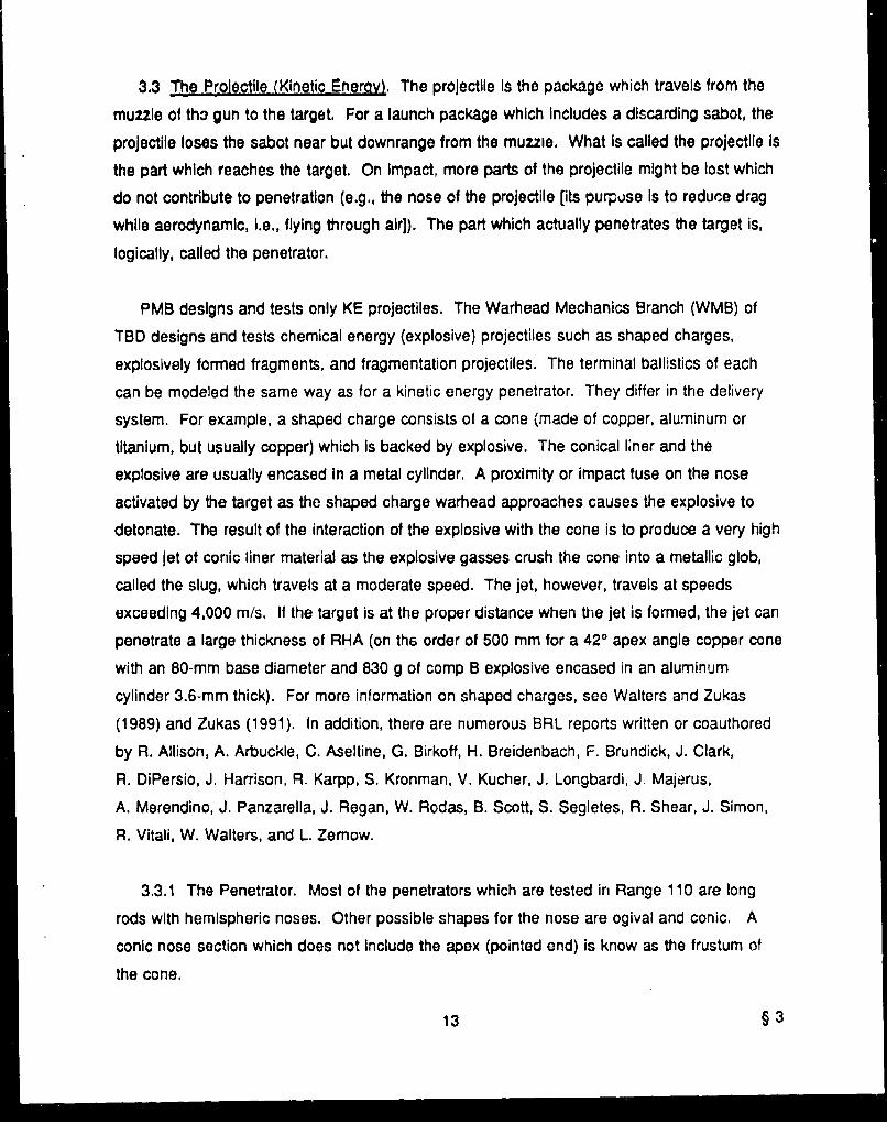
The principal reason for using the sabot assembly is that It simplifies launching penetratorswhich vary widely In size without having to change the gun system. Figure 4 shows a drawing

of a typical sabot assembly. An exploded view Is shown in Figure 5.

The mass of the entirc launch package (penetrator plus sabot assembly) is needed to

determine the proper pow,.,er curve to consult when determining the amount of propellantrequired to achieve a particular striking velocity. This value wil; also act as a check on the

other mass values recorded since the sum of the mass of the Individual parts should be closeto the value of the total mass. Figure 6 is a schematic of the launch package.

The data to be recorded with respect to the sabot assembly involve the following:

(1) the mass of the carrier,

(2) the mass of the pusher plate,

(3) the mass of the obturator, and

(4) the mass of the launch package,

It is also advisable to masure the diameter of the carrier and the diameter of the

obturator.

15 §3

45*

~b ~.a occct atn P USHER PLATE

-CARRIER (~4 SYMMETRIC SCTtONS) ,'ý

ob I -------

TRPE GROOvES <e, 5 OEPTH)

Figure 4. Diagram of a Typical Sabot Assembly.

A

2 DECREE TAPER

A 450

F A-M PUSHER PLATE

o~. CARIRIERI (4 SYMMETR[C 3rCT IONS)

TAPE GROOVES (0.1$ DETH

Figure 5. Exploded View of Sabot Assembly.

§3 16

TAPE ALSO WRAPPED HERE --

TO HOLD OBTURATORMN CARRIER TOGETHER

PENETRATO

TAPE GROOVES

MASKING TAPE OR SCOTCH TAPEWRAPPED AROUND THE CARRIERWITHIN TH GRiOOVES

Figure 6. The Launch Package.

3.4 Selecting a Striking Velocity. The first step In determining an initial striking velocity for

a particular penetrator and target configuration is to estimate the ballistic limit (the highest

striking velocity which will result in a zero residual velocity) (see the last part of this section for

a method for estimating the ballistic limit velocity). The first striking velocity should be about

250 m/s above the estimated ballistic limit (or the highest velocity obtainable).

If the result is a penetration (sometimes referred to as a partial penetration), then increase

by another 250 m/s (or as high as possible). If the result was a perforation, then select the

midpoint between that striking velocity and the estimated ballistic limit or the highest partial (if

it is greater than the estimated ballistic limit). Continue this procedure until several

perforations with small impact yaw and with measured striking and residual velocities have

been achieved. It is desirable that at least one shot result In a low residual velocity (below

400 m/s).

The accuracy in determining the actual ballistic limit Increases as the difference between

the highest penetration and the lowest perforation (sometimes referred to as a complete

17 §3

penetration) decreases. Because of differences between Impact conditions (e.g., penetrator

yaw relative to target orientation on impact), it is possible to have a penetration occur at a

velocity higher than that of a perforation. Refer to Sections 8.2 and 8.3 for on explanation of

how to handle this situation.

A method for estimating the ballistic limit a priori is given in Lambert (1978). This method

Is the following. Set z * .[.sec (0) , where T is the target thickness, D is the penetratorD

diameter, 8 is the target obliquity, and sec is the secant function (= 1/cos(e)). The ballistic

limit velocity for RHA targets car, be estimated from the following:

VL M4,000 (z .- 1) D

where M is the penetrator mass, and the units for L, D, and T are centimeters, M In grams,

and VL in m/s. The value 4,000 Is related to RHA as the target material. For other target

materials, a different value should be used. For aluminum targets (density of 2.77 g/cc), a

suggested value Is 1,750.

A discussion of the rationale behind these equations is given in Zukas et al. (1982).

3.5 Determining Time Delays. After a striking velocity has been selected, ii is necessary

to calculate the proper time delays between the trigger screen being activated and the x-ray

tu.es being pulsed. It is desirable to have the x-ray tubes flash when some part of the

penetrator is directly in front of the x-ray tube as it flashes. For station 1. it is necessary to

determine the distance along the shot line from the trigger screen to a point in front of the

x-ray tubes at station 1. At station 2. the required distance is the distance between the x-ray

tubes of station 1 and those of station 2. The time delays may then be calculated from one of

the following equations:

Time Delay (gis) = 25,400 Distance (in) / Velocity (mis),

= 1,000 Distance (mm) / Velocity (m/s).

§3 18

Calculating time delays for the stations behind the target is more difficult because the residual

velocity must be estimated. A quick estimate may be made from solving the following

equation:

v,. ~5Iv-

where V, Is the rosldual velocity, V. is the striking velocity, and VL Is the estimated ballistic

limit (see Section 3.5 for a method to estimate the ballistic imit). Then the time delays may

be calculated In the same manner as In front of the target but using V, rather than it.

Generally, It Is better to use a larger value for the distance than the distance between

adjacent x-ray tubes at stations 3 and 4 to calculate that time delay, unless those tubes are

well separated--the limitation is determined by the size of the x-ray film. However, Care must

be taken when the target is at an oblique angle because as the residual velocity approaches

0, the residual penetrator tends to exit the rear of the target at angles which approach 900

(normal) to the rear surface of the target. If the target is tilted forward (top toward the gun),

the residual penetrc-tor flies upward, away from the original shot line, downward if the target Is

tilted backward. Sometimes the deviation angle from the shot line (exit angle) is greater than

the angle of obliquity-observed with HHA targets. Therefore, account must br' taken of the

relative position of the x-ray tube, the likely location of the residual penetrator based on the

vertical component of the residual velocity, and the x-ray film location In order to insure

capturing the Image on the film.

3.6 Selectina the Amount of Propellant. The type ot propellant and the amount should

be recorded.

Variations In striking velocity are achieved by varying the amount of propellant that is

packed in the cartridge before loading the gun. The amount of propellant depends mainly on

the type of propellant used (that is, its burning rate) and on the mass of the launch package

(sabot assembly plus penetrator).

The relationship between the striking velocity and the amount of propellant needed for a

particular launch mass is reasonably linear over a wide r=nge of velocities (typical powder

19 §3

curves are shown In Figures 7 and 8). Therefore, a powder curve can be established by firing

two or three shots. The curve can then be used to estimate the propellant needed for a

particular shot. For a particular test series, points are added to the powder curve as the testprogresses and may mean that the curve must be redrawn to reflect actual conditions.

There are a number of factors involved, any of which will affect the powder curve. One of

these factors is the effectiveness of the sabot/bore Interface providing a good seal so that the

burning propellant gases do not bypass the launch package while traveling within the barrel.

This Is affected by the wear on the bore caused by each shot and by the diameter of the

sabot assembly. Another factor is how well the volumo of the cartridge case not taken up by

the propellant is packed (the burning rate of the propellant varies directly with the pressure it

experiences).

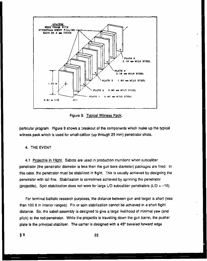
3.7 Witness Pack/Panel, Information about the behind target fragment pattern must

sometimes be recorded (depends on the purpose of the test), This information involves not

only the distribution pattern of the fragments but also the mass and velocity of individualfragments. A witness pick or panel placed behind the target is frequently used to obtain this

Information.

It Is possible to obtain this Information from flash radiographs if orthogonal views are made

behind the target-not easily done with oblique angle targets. This method has more

problems associated with it than the witness pack method and is not frequently used other

than to obtain the mass and velocity of the residual penetrator (Arbuckle, Herr, and Ricchiazzi

1973; Zook and Merrit 1983).

A single panel placed behind the target will provide the distribution pattern of the

fragments and allows estimating the size of individual fragments from the size of the hole

made in the panel. Estimates of th,, velocity and the mass of Individual fragments can be

made by using a witness pack rather than a single panel. Estimates of the mass and velocity

can then be made by examining the size ef the hole and the depth within the witness pack

that a fragment produces. The evaluation of the witness pack for any particular shot is quite

tedious and usually requires quite a bit of time. Therefore, It is used only when required for a

§3 20

41 gram rod Laaunch 401rox, X31 g1eM 16606 preveallhan

SV(D/N) - 3 . 5.11'• * S 142 Mf (#Nang)

240

* 210

2000

tao

130,

ISO-

160 •

180,

1200 300 10200 1 200 1100 2.400

VELOCXTY (M/0)

Figure 7. Sample Powder Curve for 165-mm Propellant.

as Oranl rod Launch APPOX2 242 gram 3700 §o5pollant

SV(0m/8) 43614 • 6.472 W (Vtamo)

9 0

7 0

5: 0 9 0 l c aoa 10 10 L0

VEOCTY (Mw

Fiue8 apePodrCrefr37m rplat

~2 5..•

WOOD SPACERSov RARE wi'?K

STYROFOAN SHEET ?!LLWC ---

3.18 anmIWILD STEEL

- " // " "PLATE 4

PLATE 3 1.-60 MW MI LD STEEL1.22

PLATE 2 0.80 mm WILD STEEL

'- PLATE 1 0.50 . WILD STEEL0.41, m .b4..-

Figure 9. Typical Witness Pack.

particular program. Figure 9 shows a breakout of the components which make up the typical

witness pack which is used for small-caliber (up through 25 mm) penetrator shots.

4. THE EVENT

4.1 Projectile in Fliaht. Sabots are used in production munitions when subcaliber

penetrator (the penetrator diameter is less than the gun bore diameter) packages are fired. In

this case, the penetrator must be stabilized in flight. This is usually achieved by designing the

penetrator with tail fins. Stabilization is sometimes achieved by spinning the penetrator

(projectile). Spin stabilization does not work for large L/D subcaliber penetrators (L/D > -10).

For terminal ballistic research purposes, the distance between gun and target is short (less

than 100 it in interior ranges). Fin or spin stabilization cannot be achieved in a short flight

distance. So, the sabot assembly is designed to give a large likelihood of minimal yaw (and

pitch) to the rod penetrator. While the projectile is travelling down the gun barrel, the pusher

plate Is the principal stabilizer. The carrier is designed with a 450 beveled forward edge

§5 22

(beveled inward) so that, exterior to the gun, the aerodynamic forces acting on the bevel will

force the petals of the carrier to separate early In flight. In some cases, sabot separation is

accelerated by firing through a thin sheet of foam, although passing through the foam often

has a destabilizing effect.

The pusher plate follows along behind the penetrator and usually Impacts the target at the

entrance hole made by the penetrator. Analysis of the appearance of the entrance hole

should take this into account. If It is desirable to eliminate the effect of the pusher plate

Impact, a deflector set up in front of the target will cause the pusher plate to deviate from the

shot line. One method is to position the edge of a metal block so that the pusher plate clips

the block. A method which has been tried is to use a metal plate with a hole large enough to

allow the penetrator to pass through but not large enough for the pusher plate. This method

Is not generally successful because the penetrator becomes destabilized in passing through

the hole, even though care is taken to align the hole with the shot line.

4.2 Impact. At medium to high striking velocities (above a few hundred meters per

second) Impact, metal penetrators impacting metal targets produce a brilliant light source

during the penetration process. For this reason, optical cameras cannot be used to record the

actual penetration process. That is why ballisticians have resorted to flash radiographs. The

film used In the flash radiograph is protected from exposure to the light source by being

placed in a cassette which is made from either wood or cardboard. The x-rays can easily

penetrate through the film cassette and expose the film (generally, the exposure is enhanced

by using an image intensifier screen directly in front of the film). Images are formed whenever

the x-ray radiation is attenuated by absorption in intervening material such as the metal

penetrator or metal target.

Metallic penetrators which strike "soft" metallic targets such as 2S-O aluminum (-BHN 25)

can deform but do not lose mass to the penetration process at low to moderate striking

velocities (under 1,000 m/s). This mode of penetration is called constant mass penetration. It

the penetrator has a pointed nose, there might not be any observable deformation of the

penetrator, In which case, the penetration is that of a rigid body.

23 5

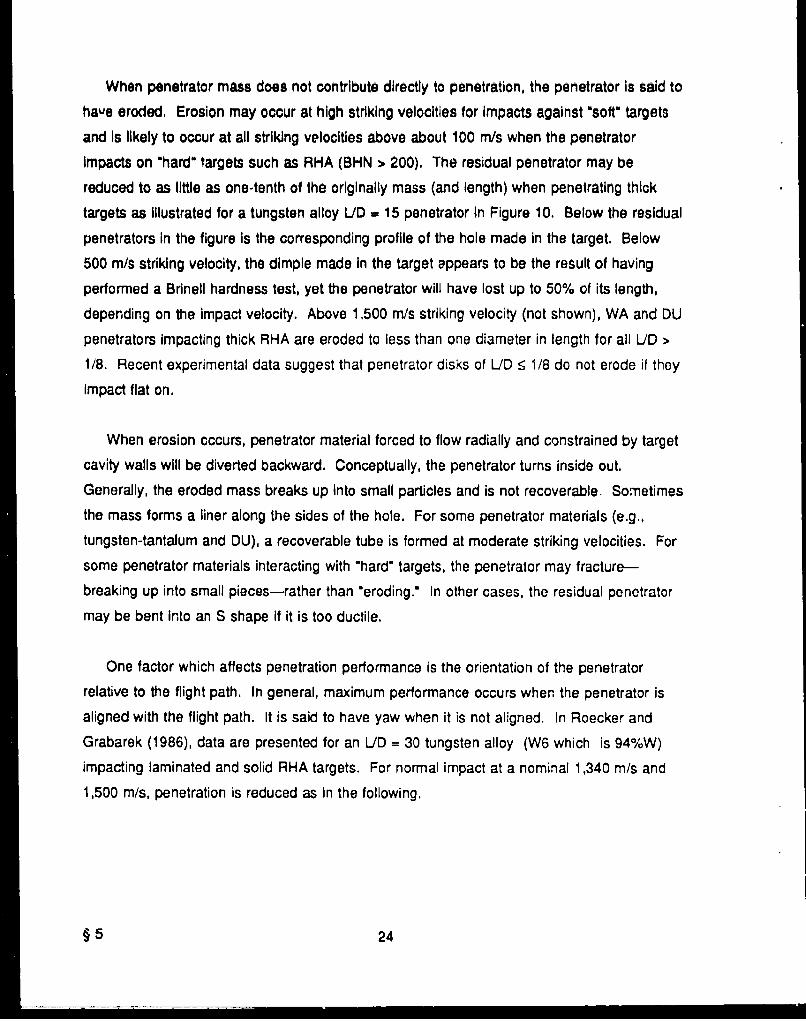
When penetrator mass does not contribute directly to penetration, the penetrator is said to

have eroded, Erosion may occur at high striking velocities for impacts against "soft" targets

and is likely to occur at all striking velocities above about 100 m/s when the penetrator

Impacts on "hard" targets such as RHA (BHN > 200). The residual penetrator may be

reduced to as little as one-tenth of the originally mass (and length) when penetrating thick

targets as illustrated for a tungsten alloy LID - 15 penetrator in Figure 10. Below the residual

penetrators in the figure Is the corresponding profile of the hole made in the target. Below

500 m/s striking velocity, the dimple made in the target appears to be the result of having

performed a Brinell hardness test, yet the penetrator will have lost up to 50% of its length,

depending on the impact velocity. Above 1,500 rn/s striking velocity (not shown), WA and DU

penetrators impacting thick RHA are eroded to less than one diameter in length for all L/D >

1/8. Recent experimental data suggest that penetrator disks of LID < 1/8 do not erode if they

Impact flat on.

When erosion occurs, penetrator material forced to flow radially and constrained by target

cavity walls will be diverted backward. Conceptually, the penetrator turns inside out.

Generally, the eroded mass breaks up into small particles and is not recoverable Sometimes

the mass forms a liner along the sides of the hole. For some penetrator materials (e.g.,

tungsten-tantalum and DU), a recoverable tube is formed at moderate striking velocities. For

some penetrator materials interacting with "hard" targets, the penetrator may fracture-

breaking up into small pieces-rather than "eroding." In other cases, the residual penetrator

may be bent into an S shape if it is too ductile.

One factor which affects penetration performance is the orientation of the penetrator

relative to the flight path. In general, maximum performance occurs when the penetrator is

aligned with the flight path. It is said to have yaw when it is not aligned. In Roecker and

Grabarek (1986), data are presented for an L/D = 30 tungsten alloy (W6 which is 94%W)

impacting laminated and solid RHA targets. For normal impact at a nominal 1,340 m/s and

1,500 m/s, penetration is reduced as in the following.

§ 5 24

L/D=15 WA VS. KIa RESIDUAL LENGTH AND TARGET HOLE PROFILES

V. 0 200 400 600 800 1000 M/0

10%O 85% 6F1 30% 16% 12XLs

P, 0% 1% 2% 4% 12 33%Le

Figure 10. Erosion of Tungsten Alloy Penetrators Impacting RHA.

% ofyaw angle penetration

(%) at 00 yaw

0 1001 982 913 814 71

Data are also shown for oblique impacts of 600, 650, and 70,50. These data suggest that If

the pitch (yaw angle in the vertical plane) of the penetrator is away from the target surface

(effectively increasing the obliquity), penetration is degraded quite rapidly. Penetration is noi

degraded as rapidly when the pitch is into the target (effectively reducing the obliquity).

Taking the 650 obliquity case, for example, penetration is about 79% with a pitch of -1.50 or

+3.00 where the minus pitch is away from the target. For the 70.50 obliquity, penetration is

degraded very little for pitch angles from -0.50 to +2.00.

25 § 5

For normal Impact (00 obliquity), an explanation for the effect of yaw on penetration

performance Is presented In Bjerke ew a]. (1991), They present evidence to support the theory

that a critical yaw angle exists fcr eacih .enetrator/target configuration. For yaw angles less

than the critical yaw angle, there is no dep~adation In penetration performance. The critical

yaw angle is that angle of yaw which allows the side of the penetrator to interact with the wall

of the cavity being formed. The equation to compute this critical yaw angle (attributed to

Silsby, Roszak, and Giglio-Tos 1983) Is as follows:

YXr = sin' 1 2L(1)

where Dh is the entrance diameter of the hole in the target (measured in the plane of the

original target surface), DP is the penetrator diameter, and L is the penetrator length.

The hole diameter can be computed from the ratio Dh/D,, which can be approximated by

the following equation:

Dh V + V+ . (2)

S3 8

The equation given in the report differs primarily in the value calculated for V = 0, which is

1.1524 in the report rather than 1. V represents the striking velocity in kilometers per second.

Since the hole diameter in the target is dependent on material properties of both the

penetrator and the target, Equation 2 applies to WA vs. RHA only. A more general solution,

which is dependent on material properties, is the following:

Dh (X PVo _ Uo )2 . P1 U2S1 (3)

DP 2H

V -0 - V,) 2 1(i -p ) H - Y

U0 2 P1 for la # 1 , (4)

§5 26

UO o V H -HY forp- 1, (5)2 p•,Vo

where V. is the striking velocity, p, and p, are the penetrator and target densities, respectively,H Is the target resistance, Y is the penetrator flow stress, g' - p/p,, and X = 3.6 (% depends to

some extent on the size of the hole made in the target). For example, using MKS units, let

Vo - 1,500 m/s, pp = 17,300 kg/m3, p, = 7,850 kg/rn 3, H = 5.5 x 10' pascals, and Y = 1.9 x 109ps.-ý: Is, then p = 0.4538, Uo -701 m/s, and DWDP = 1.99. With Equation 2, the result Is 1.78

and using the equation from the report, the result Is ';.95 for V = 1.5 km/s. Neither Equation 2

or 3 accurately reflects the hole diameter obtained experimentally at low striking velocities

(below -400 m/s for WA vs. RHA).

Returning to Bjerke et al. (1991), once the critical angle is computed, the degradation in

penetration can be computed from the following:

piu, p M Cos 11.46Y (6)

where Prn, is the penetration for a WA penetrator with yaw angles less than y,. (Note: The

cosine function should be evaluated with the argument in degrees.) For a DU penetrator, the

equation to be used is as follows:

P Pm" Cos 9.457 ', (7)

Nonzero yaw will also affect the performance against finite thickness targets. The yaw onimpact as observed from the flash radiographs in experimental work should be taken into

account when deciding what residual velocity data .-nould be used in evaluating a velocity

ballistic limit. What adjustments can be made to the residual velocity to make it equivalent towhat would be obtained with 00 yaw has not been determined yet.

27 § 5

5. RADIOGRAPHIC ANALYSIS

5.1 The Magnification Factor (K-Factor), The x-ray radiation which is produced by thex-ray tube emanates as though from a point source. That Is, the space that the radiation

travels In appears to be a cone with the tip of the cone (apex) located at the sourco end of thex-ray tube. Since the projectile Is located between the x-ray tube and the film at the time thex-ray tube flashes, th3 image that Is produced on the film is larger than the projectile. The

closer the projectile Is to the film, the less will be the magnification. From the geometry of therange setup, the magnification factor (K factor) can be calculated from distances measured on

the film. These values can then be multiplied by the K factor to produce adjusted values

which represent the actual location of the projectile in space.

The following is a derivation of the K factor based on the diagrams shown in Figures 11and 12. Figure 1 i represents one station In which there are two x-ray tubes--one horizontal

and one vertical. A .hree-dimensional view is shown in Figurc 12 (Grabarek and Herr 1966).

Let Xh, and Yhf m X-ray tube head to film distances in X and Y directions, respectively,

X. and Y, = Fiducial line (z-axis direction) to the orthogonal film plare distance.X, and Z_ # Coordinates of an image point on the horizontal (X-Z plane) film.

Y, and Z,, =s Coordinaies of a corresponding image point on the vertical (Y-Z plane)

film.

XP, YP, and Z, _* Actual physical coordinates of the point in space.

The origin of the coordinate system is located at the point of intersection of both filmplanes with the X-Y plane In which both x-ray tubes are located. The following equations are

derived based on the geometry:

Y hf Y Ph W- (8)X-x X,-X

Xhf XpT (9)Y-Y Y-Y

§ 5 28

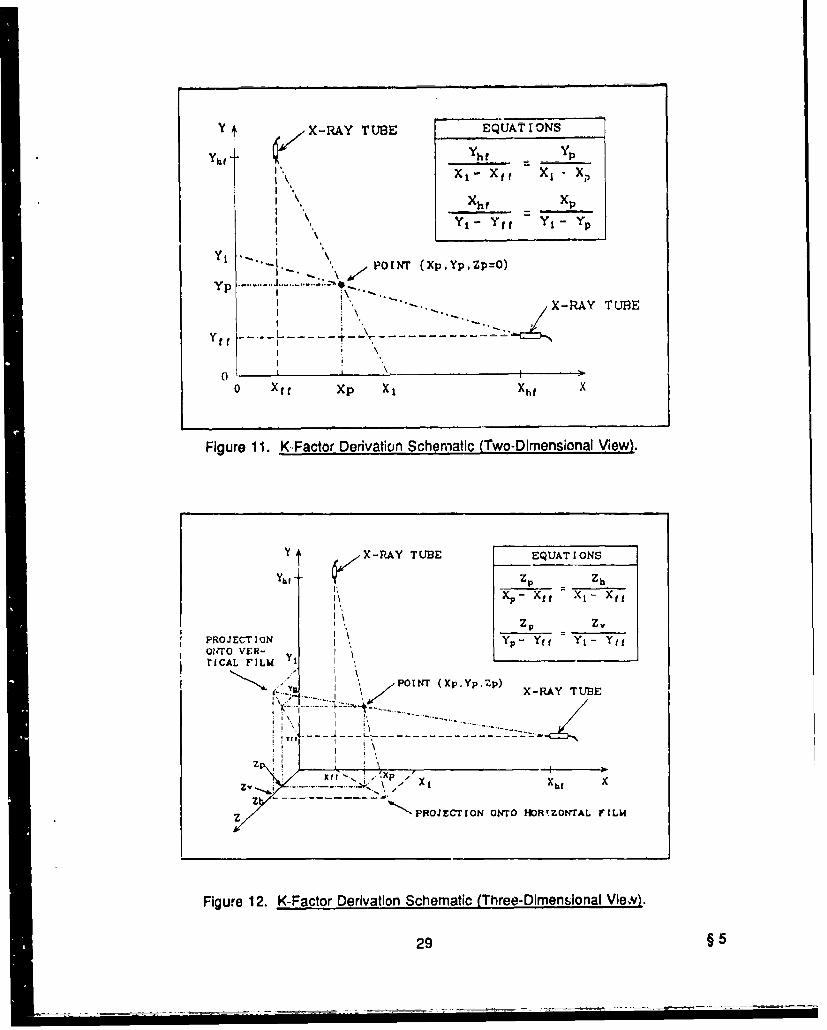
Y X-RAY TUB3E EQUAT IONS

Yh Y~hf .... o

iXl- Xtf XI - XpI,I \ Xhf Xp

Y - Yff Yt Yp

"" -- POINT (XpYpZp=O)Y l ......... ......... .

X-RAY TURE

y f f - - - - _-\- - - - - - - - -

0 •0 X~f Xp XI Xhf x

Figure 11. K Factor Derivation Schematic (Two-Dimenslonal View).

Y 7 X-flAY TUBE EQUAT IONS

Yla • Zp Zh]-h

\X~p - Xt Xt- X tI

I\.Zp Z

PROJECTION t Yp- Yff Y 1 - Yf 1ONJTO VER-rICAL FILM Y, '

POINT (Xp.YpZp) X-RAY TUBE

-I .

S-------.-- ' O...O

z .PXWROJECTION ONTO HWRZONTAL FIL,

Figure 12. K-Factor Derivation Schematic (Three- Dimensional VieNj.

29 §5

__ i_ . __ .. ,( O)XP - Xtt X1 - X4

Z _Z,, (11 )

YP =Y11 Y;V- Y, '

Solving Equation 8 for Xp and substituting In Equation 9 yields the following:

Xhf _Yhf s -4+ YP X,1-"-YOX 1 (12)Y, - Ytt YhfY1 - YhfYP

Cro.ss multiplying, expanding, and then solving for YP,

Xh=YhIYI *f ' YhfYtf X - Yh,XI Y1

Xhf Yhf * Xf Y1 + Yf X1 - Xff f - Xi y1

The magnification factor in the Y-Z plane (vertical plane) can be defined as follows:

KV or using Eq:jatlon 1" , K -W Y _ Yf ' (14)

Replacing Y, of Equation 14 with the right side oi Equation 13 and collecting terms,

SXht Yht - YhX1 + Y X1 - XY(15)X1fYhf - (X,- X0) (Y, - Yff)

The magnification factor in the horizontal plane (X-Z plane) can be found in a similar manner.

That is, solve Equation 8 for YP and substitute In Equation 9. Cross multiply, expand, and

solve for X1 . Use _-quation 9 to find an expression for K,,, which Is as follows:

Kh Y XP - X11 (16)

X1 - Xff

§ 5 30

Substitute the expression for X. to obtain the following:

Kh M Xhf Yh.. - Xh YV + X1, YV - X1f Y11 (17)hXhYhf - (X; - R;5 (V1 " Y) (

It is easier to measure on the film the distances XY-X4 and Y1-Yf. Therefore, let

X=XI-X4 andY=Yi-Y1. (18)

Then tie vertical magnification factor may be expressed as follows:

KV a Yh,(Xhf - X,,) - (Yhf - YO) X (19)

XhfYh! - X Y

and the horizontal magnification factor is as follows:

Kh - Xh' (Yhf - Yff) (Xhf - Xff) Y (20)SXhI'4? - X Y

The sign convention is that the X distance Is positive if further away from the vertical film

plane than the fiducial line on the horizontal film and negative if the point is closer than the

fiducial line. Similarly, the Y distance is positive If the point on the vertical film Is further away

from the holzontal film plane than the fiducial line on the vertical film and negative It closer.

If X1, = YV, Xv = Yf, and X = Y. then the horizontal and vertical magnification factors have

Identical values. Assuming that X,, and Yhf are both 60 In and that X4 and Y. are both 8 in,

then K., K, = 0.8667 when X and Y are both 0.

To make the adjustment to the X, Y, and Z values measured on the film, those values are

multiplied by the appropriate K factor to obtain the coordinates of that point in the physical

space bounded by the film planes and the respective x-ray tubes. The velocity can be

31 § 5

computed based on the distance calculated In physical space and the time delay between the

x-ray tube flashes at adjacent stations. Also, the angle of travel can be determined.

The magnification factor Is usually computed for only one x-ray station in front of the target

and then used for all adjustments from film measurements to physical space coordinates.

This x-ray station must have two tubes which are orthogonal to each other and an image of

the projectile obtained In both film planes. For oblique angle impacts, it is not feasible to have

a vertical x-ray tube at the station directly in front and the station directly in back of the target

since the target blocks the view. The other reason that the magnification fartor is Comiputed

only once is that the penetrato, is assumed to exit the target in the same vertical planci as it

entered the target and the magnification factor does not change.

From the film that was in the vertical plane, a point on the image Is selected, which can be

identified on the Image from the film in the horizontal plane. For example, the center of the

front end or a point can be assumcd to be the center of mass. The distance from the fiducial

wire Image, which is parallel to tho shot line, to the selected point is the Y value (positive if

above the fiducial, negative If below). From the film that was in the horizontal plane, the X

value is measured in the same way (positive if the point is further away from the vertical film

than the fiducial wire image, and negative if closer). The values are substituted in Equation

19 to obtain the vertical magnification factor. The distances Xh Yh,, Xe, and Y. must, of

course, be known and measured in the same units as used for X and Y. A typical value for K.,

is 0.866/, as mentioned before.

5.2 Striking Velocity. Measurements on the radiographic film are made using a

transparent plastic ruler which is calibrated in two hundredths of an inch (or 1/2 mm). Working

with the fitm which was vertical at station 1, a point is selected which is located on the image

of the projectile (for example, the center point of the front tip). Measurements are made with

respect to the fiducial line images which were directly in front of the x-ray tube at station 1.

The distance Y1 Is measured from the horizontal fiducial line image to the selected point on

the projectile Image. If the selected point is above the horizontal fiducial line, the

measurement is positive, otherwise, It is negative. The Zi value Is the measurement from the

vertical fiducial line to the selected point on the projectile image. This value Is positive if the

selected point is further from the gun than the vert!cal fiducial line Image, negative If closer.

§ 5 32

The same procedure Is followed for the Images related to station 2 to obtain Y2 and 4.Letting Z, represent the separation between stations I and 2 In the Z direction, K, represent

the magnification factor evaluated from the equation In Section 5.1, and At represent the time

delay between the flashes at stations 1 and 2, the striking speed can be calculated as follows:

Ayd - K, (Y 2 - YJ), (21)

AZd - K, (Z2 - ZO) + Zh., (22)

/-y + A ZIV,. W dE d, (23)

where V. is the striking speed. Strictly speaking, 0e X value from the horizontal film should

be adjusted and Included in Equation 23, but it ha3 such little effect on calculating the velocity

that it Is neglected. Since measurements are usually done In inches, the result of Equation 23must be divided by 12 to convert to feet, and since the time delay is usually recorded in

microseconds, the result must be multiplied by 1,000,000. This will give the speed in feet per

second. To convert feet per second to meters per second, the result must be multlpI!ed by0.3048. The conversion factor, 0.3048, Is an exact value (i.e., no error is introduced in

making the conversion).

5.3 Yaw and Pitch. It Is unusual for the projectile to fly perfectly straight. The projectile Is

said to have pitch if It is tilted up or tilted down. It has yaw if it Is turned sideways any amountwith respect to the flight path. Sometimes, yaw is used In a loose sense and Includes the

pitch. In this case, the distinction is made between horizontal yaw and vertical yaw. The

angle wHich the projectile's center axis makes with the flight line Is called total yaw. How total

yaw can be calculated from horizontal yaw and pitch will be shown later.

The method for determining the yaw or pitch from the film used In a system where there is

certainty that the fiducial lines are aligned with respect to the gun, shc ne, and the x-ray

tubes Is as follows. A tine is drawn either on the centerline of the projectile Image or along

33 §5

one edge and extended until it intersects a fiducial wire Image which is perpendicular to the

flight path direction. A protractor Is then used for measuring the angle (in degrees) made by

the Intersection of the line drawn and the fiducial. For pitch, the angle is positive if the

projectile Is tilted up, negative If tilted down. For horizontal yaw, the angle is positive if the

projectile Is twisted to the right when looking toward the direction of travel and negative if to

the left.

Accurate measurements of the yaw and pitch are dependent on how well the fiducial wires

are aligned after installing the film cassettes. Extra care must be taken when installing the

film cassettes because the fiduclal wires frequently catch on the surface of the cassette and

get misplaced. Also, the wire that Is used Is similar to piano wire and can develop kinks. This

makes It difficult, when examining the x-ray film, to determine how the fiduclal wire image

would have been if the wire had been straight.

A method for determining the yaw and pitch which Is independent of the fiduclal lines Is

the following. Establish a point representing the center of mass on each Image (see the next

subsection for mathematically determining the location of the center of mass). Draw a straight

line connecting the center of mass of each image. Draw a line parallel to the side of an

image and determine the angle that this line makes with the line drawn through the centers of

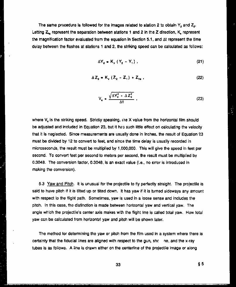
mass. This can be done with a protractor, or possibly more accurately, by measuring

distances as shown in Figure 13 and calculating the arc tangent (easily done with a scientific

calculator-arc tangent is usually abbreviated by ATN or by tan*'). An angle computed in

radians can be converted to degrees by multiplying the value in radians by 180/3.14159

(= 180/x).

Yaw and pitch are Important considerations when trying to analyze shots made against

targets which are at oblique angles to the shot line (not perpendicular). Penetration

performance may be enhanced slightly If the angle formed by the centerline of the projectile

and the target impact surface is slightly less than angle of obliquity. Otherwise, penetration

performance is degraded because there is more projectile area presented to the target. The

longer the projectile, the more critical this is. The worst performance for long projectiles will

occur when the projectile impacts sideways (900 yaw or 900 pitch for 0 obliquity targets).

§5 34

LINlE PARALLEL TO

THE IMAGE ED,•E

LINE T-WUrUH THE

MOND IVA= cENTERs or wAss

TiRsT ibWGE .d 6

.. _.._...... ......

LINE~ PARALLEL To THELINE TIUROUH THE

S o•EEVrS or N•=

TAN d OTA

Figure 13. Pitch or Yaw Calculation Without Fiducial Wire Reference.

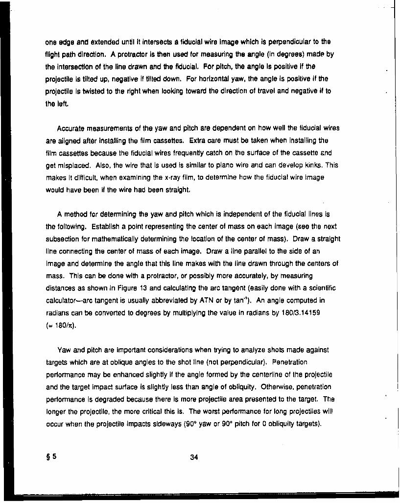
The total yaw angle may be computed from 'he two components-yaw and pitch.

Figure 14 shows the Identification of the angles. In this figure, the angle a is the pitch, the

angle P3 is the horizontal yaw, and the angle y is the total yaw angle (angular deviation of the

nose of the penetrator from the flight path determined at the center of mass of the projectile).

The trigonometric identities are as follows:

Y

TAN (ax) = (24)

z (5TAN (13) = ., (25)

and

TAN (y) x (26)

35 §5

Y •, r(Yo* ZI)

BASIC EQUATIONS-/./. - TAN d•= Y/X

.- A A\ I .A Z/X

-iTAN r -~(yo 4ze)X X

", i/ BY SUSTITUTrION

TAN ,, TANd + X1 TANSB

TAN r =(TAN 2 d + TAN2)

FOR S14ALL ANGLES, THE APPROXIMATION IS0 2 f(ci+ B2)

Figure 14. Combining Pitch and Yaw to Obtain Total Yaw Angle.

By substitution,

TAN(y) V(XTAN((a))2 + (XTAN(p) 2 (27)

The X2 may be extracted from the argument of the square root function which will cancel

the X in the denominator. The result is as follows:

TAN(y) w V(TAN(a))' . (TAN(p)) . (28)

When the angles are small-less than 20, the following approximation may be made;

y - V12 *+ 1.(29)

For a description of the Influence of the yaw angie on penetration performance, refer to

Section 4.2.

§5 36

5.4 Center of Mass. The center of mass of a physical object is the geometric point within

the object which behaves as though all of the mass were concentrated at that point when the

object is subjected to external forces, A more rigorous definition Is the following:

If an arbitrary set of forces acts on a rigid body, the center of mass of the body will

move as if all of the mass and all of the forces were concentrated at the center of

mass (Ference, Lemon, and Stephenson 1956).

For a sphere of uniform density (homogeneous) or a sphere made up of concentric shells,

each shell made of material of uniform density, the center of mass Is the center of the sphere.

The center of mass for a right circular cylinder of uniform density is the midpoint (L.2, D/2),

where L is the length and D is the diameter.

The center of mass of an object made up from several different geometric shapes can be

found by first finding the center of mass of each individual geometric shape. Then the

individual centers of mass are combined, as will be demonstrated In the following section

contributed by Graham F. Silsby.

5.4.1 Location of the Center of Mass of a Hemispherical Nosed Right Circular Cylinder.

Symbols: L ,. overall length of rod

D * diameter of rod

m , mass

p = density (assumes rod is of uniform density)

v = volume

z , distance measured from the tail erd toward the nose.

Subscripts (see Figure 15): c * cylinder

cm = center of mass

i Ith term

h = hemisphere.

37 §5

S• ZCM , M SPHERICNOSE

T L/2 - >

.. L --

Figure 15. Location of Center of Mass of a Hemispheric Nose Rod.

Derivation: By definition, for any solid comprised of different geometric sections of uniform

density,

zC llErW E pv,a A

where the subscript i denotes the ith secton. For the right circular cylinder portion, the center

of mass relative to its base (noting that L is th9 overall length of the heminosed rod) is as

follows:

The volume of the right circular cylinder portion is as follows:

§5 38

For a hemisphere, the center of mass relative to Its base is as follows (Oberg, Jones, and

Holbrook 1979):

3D8 2

The center of mass of the hemispheric nose portion relative to the tall end of the rod is as

follows:

Zh W L - 3D2 16

The volume of the hemisphere is as follows:

2 D:' 7tD 3"v d -3 8 1"-2"

Therefore,

I L ) ' D L - ) + ( 3 D ) x D

nD D 2 L(tD

Cancel out nD2/4 and consolidate separate terms. Then,

1L D (L 5DL

L- D

Substituting D (LID) for L and simplifying results in the following:

1zL _ 1[22l+ I (]

which is valid for all LID > 1/2.

39 §5

Example: Let L = 195 mm and D 6.5 mm so that L/D 30. Then,

(29.5)2 + 29.6875

Z&" a 6.5 --_2 ..... .3 1 96.96 .29.8333

Since L/2 = 195/2 - 97.5, the center of mass is 0.54 mm toward the tail end from the center

point of the overall length. The following will show that for all L/D > 3, the center of mass Is

located very near D/12, behind the center point of the overall length.

Let z_

Substituting the expression for z•, and simplifylng results in the following:

1- I4LA ,, D D 4 D D

112Lý-2 12 - ?-D L

In the limit, as LID goes to infinity, A goes to D/12. T,:s is shown in Table 4.

For short hemispheric riose rods, the center of mass is near the midpoint of the overall

length. For long rods, •he center of mass is near the midpoint of the cylindrical portion of the

rod. The cylinder midpoint is always D/4 behind the center of the overall length. Therefore,

the displacement between the center of mass and the overall midpoint increases with overall

length

5.4.2 Location of the Center of Mass of a Conical Nosed Right Circular Cylinder.

Symbols: L = overall length of rod

D ,. diameter of rod

N =. length of the conic nose (cone height)

m =s mass

p * density (assumes rod is of uniform density)

§ 5 40

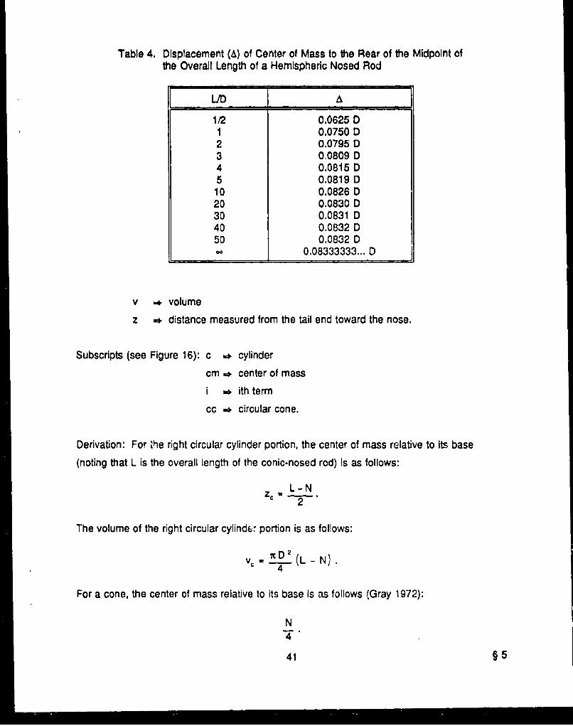
Table 4. Displacement (A) of Center of Mass to the Rear of the Midpoint ofthe Overall Length of a Hemispheric Nosed Rod

L L/D .. A

1/2 0.0625 D1 0.0750 D2 0.0795 D3 00809 D4 0.0815 D5 0.0819 D10 0.0826 D20 0.0830 D30 0.0831 D40 0.0832 D50 0.0832 D

0.08333333... D

v . volume

z ,, distance measured from the tail end toward the nose.

Subscripts (see Figure 16): c . cylinder

cm ,, center of mass

i =. ithterm

cc * circular cone.

Derivation: For 'he right circular cylinder portion, the center of mass relative to its base

(noting that L is the overall length of the conic-nosed rod) is as follows:

L-N2

The volume of the right circular cylindc6 portion is as follows:

vc= D.-2(L - N).4

For a cone, the center of mass relative to its base is as follows (Gray 1972):

N

41 5

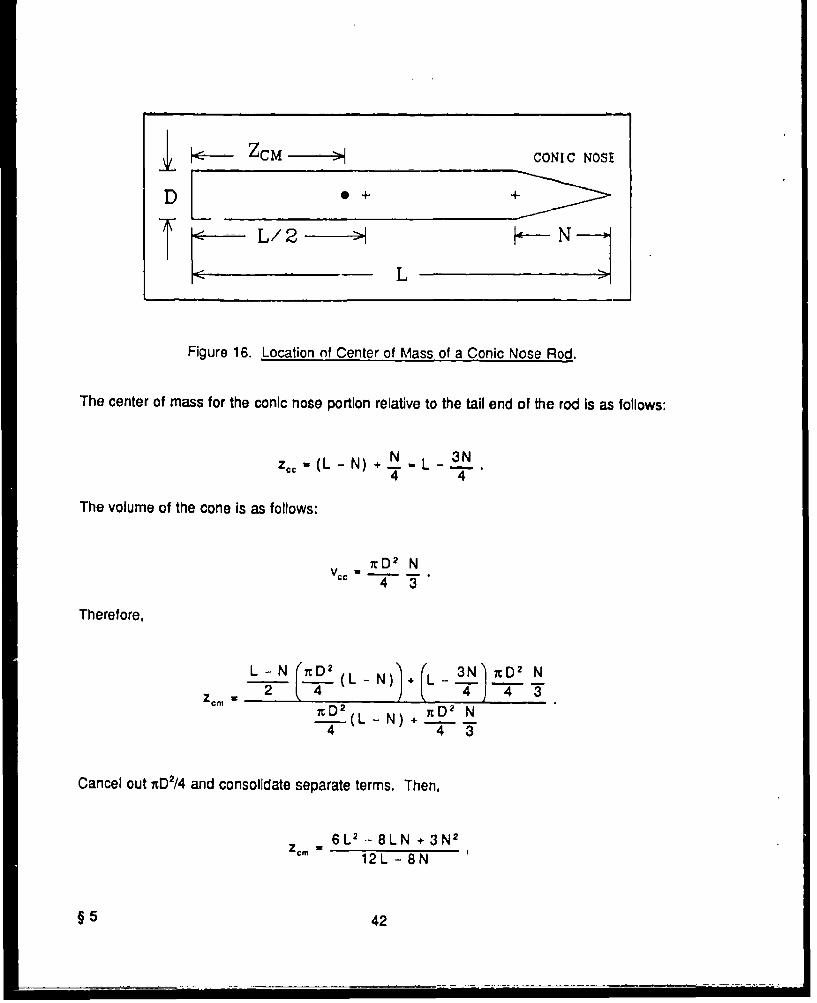
• "7 CONIC NOSE

-L

Figure 16. Location of Center of Mass of a Conic Nose Rod.

The center of mass for the conic nose portion relative to the tail end of the rod is as follows:

z,,(L - N) + N L - 3N4 4

The volume of the cone is as follows:

•rD2 N4 3

Therefore,

ZCm W 2 42 4 3L t(?D2 (L )> 3 ND 2 Nc(1. (L N) nD' N

4 43

Cancel out nD2/4 and consolidate separate terms. Then,

6L' - 8LN +3N 2

Zcm 12L - 8N

§5 42

which is validforallL > NandforL=N if N>0 Let A - -L .

Substituting the expression for z. aria simplifying results In the following:

4LN - 3N2

12L - 8N

Dividing the numerator and denominator by D results In the following:

4L N 3 N2

A W D D

1PL 8N12U _8ND 0

In the :lmlt, es IJD goes to Infinity, A ges to N

as N goes to 0, A goes to 0; and

as L goes to N, A goes to N4

Some additional values for A are listed in Table 5.

5.4.3 Location of the Center of Mass of a Conical Frustum Nosed Right Circular Cylinder.

For rods which have conic-shaped noses, the nose is not usually a full cone. Generally, the

tip end Is cut off. The name given to that geometry is frustum of the cone. This Is illustrated

in F!gure 18.

Symbols: L s, overall length of rod

D , diameter of rod

n , length (height) of the frustum of the cone

d , diameter of the tip end of the frustum

m a mass

p * density (assumes rod is of uniform density)

43 § 5

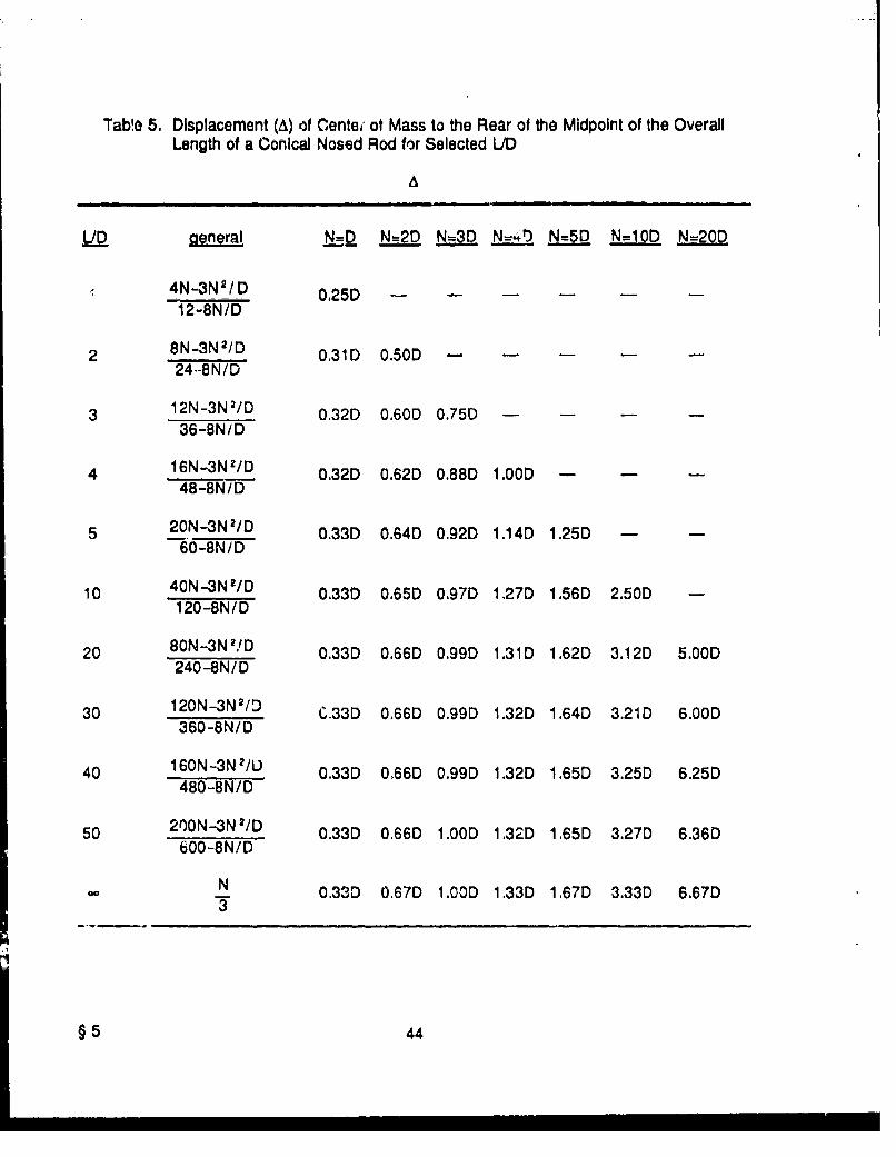
Tab!e 5. Displacement (A) of Centei ot Mass to the Rear of the Midpoint of the OverallLength of a Conical Nosed Rod for Selected L/D

A

LID cameral N=D N--2D N=3D N=,,f N=5D N=10D N=20D

4N-3N /D 0,251 2-8N D

2 8N-3N2/D 0.31D 0.501)24.-8N/D

3 12N-3N2/D 0.32D 0.60D 0.75D -

36-8N/D

4 16N-3N2/D 0.32D 0.62D 0.88D 11.00)D48-8N/D

5 20N-3N2/D 0.33D 0.64D 0.92D 1.14D 1.25D60-8N/D

10 40N-3Nz/D 0.33D 0.65D 0.97D 1.27D 1,56D 2.50D -120-8N/D

20 80N-3N!.'D 0.33D 0.66D 0.99D 1.31D 1,62D 3.12D 5.00D240-8N/D

30 120N-3N2 /D C.33D 0.660 0.99D 1.32D 1-64D 3.21D 6.00D360-8N/D

40 160N-3N 2/L) 0.33D 0,66D 0.99D 1.32D 1.65D 3.25D 6.25D480-8N/D

50 200N-3N2/D 0.33D 0.66D 1.00D 1.32D 1.65D 3.27D 6.360600-8N/D

_ N. 0.33D 0.67D 1.001D 1.33D 1.67D 3.33D 6.67D3

§5 44

V -6 volurre

z ., distance measured from the tail end toward the nose.

Subscripts (see Figure 17): c u* cylinder

cm -.. center of mass

I .a ithterm

f . frustum of the cone.

The center of mass of the cylindrical portion Is - _.2

The voiume of the cy'!ndrlal portiorn Is nD.I (L- n),4

The center of mass of a frus',.im of a cone along the center axis Is as follzws (Gray 1972):

The center of mass of the frustum nose relative to the base of the rod is as follovw:

Zf U L - n + n ((D + d)2 + 2d 2)4 ((D + d)-' - Dd)

The volume of the frustum of a circular cone is as follows:

v n D' •+ Dd + d2

(7-n D2LSetting 0- LL _....4(L -n))

2

and( n+n ((D + d) o + 2d2 I .n rD2 + Dd+d

Q 2 L -)2n Ed - 3

45 §5

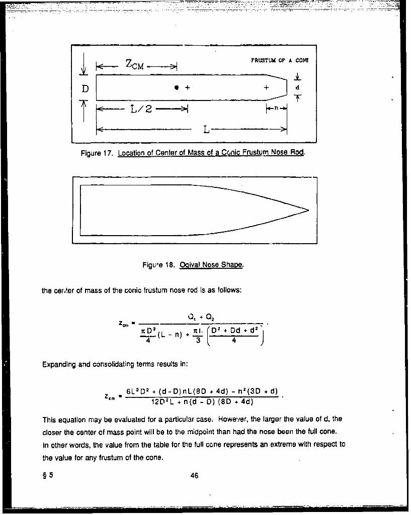
S.. .- --.. . . .

L ZCM FAUTULM OF A CONE

D + d

Figure 17. Location of Center of Mass of a Conic Frustum Nose Rod.

Figure 118. O0-l.ival -Nose Shape,,

the cei*ter of mass of the conic frustum nose rod is as follows:

7rD• 2 L n)+ . (DI + Dd +*d2

Expanding and consolidating terms results In:

6L 2D 2,+(d-D)nL(SD +4d) - n 2(3 D +d)zCM z 12 D 2L + n(d - 0) (8 D + 4d)

This equation may be evaluated for a particular case. However, the larger the value of d, the

closer the center of mass point will be to the midpoint than had the nose been the full cone.

In other words, the value from the table for the full cone represents an extreme with respect to

the value for any frustum of the cone.

§5 46

A similar analysis may be made for a penetrator with an ogival nose. The equation for the

ogive of a penetrator with nose length N is as follows:

r a R cos "n ),(2N)

where R Is the maximum radius of the penetrator (at the base of the nose) and r is the

distance from the center axis of the penetrator to the curved surface at point n where n ! 0 at

the base and n = N at the tip (see Figure 18 for an example of an ogival nose penetration

shape).

To a close approximation, the curvature of the ogive is given by the arc of a circle of

radius R&, where the center of the circle lies on an extended line from the base of the nose

section. The radius of the circle is given by the following:

R2 .N 2

R,- 2R

as shown in Figure 19.

5.5 Penetrator Residual Velocity. In general, more effort is required to determine the

residual velocity than the striking velocity. The projectile has a definite known shape, and the

image on the film in front of the target may readily be identified, as shown schematically in

Figure 20. During the penetration process, the penetrator is deformed and loses mass

through "erosion." Generally, enough of the tail end of the penetrator emerges 1rom the target

intact and undeformed so that the residual penetrator can be identified. In adUition to the

residual penetrator, there will be images of numerous other fragments, some of which are

penetrator material, but most are target material.

Analysis of the images behind the target becomes more difficult if the time delays for the

sequence of flashes behind the target are ill ..hosen. The fragment fror't forms an expanding

cone with the apex of the cone at the exit point on the rear surface of tie target. If the tir;me

delay to the first flash behind the target is too short, the fragments will be close together

(including the residual penetrator) so that It will be Impossible to pick out the image of the

residual penetrator. If the time delay to the first flash behind the target is too long, the

47 § 5

h.dARC O CIRCLE OF' RADIUS RCwhere

~2Rp3 RI R• ÷ N

RP 3 so thaty 2 r" RpCOS[iriS-- R C= 1.5

2.. Ir R p Co

.5

N 90 ' 4

0 2 4 6 8 10

xSto center of circle at (0,-li)

Figure 19. Comparison of an Qiive to the Arc of a Circle.

VERTICAL X-RAY FILM

rIDLCIAL

UL•OkiD lilas" OF

=In-tA". Pm;HtT1tATOA

rPIWT IM"Gz orRESIDUAL PENPRATOR

CONTINUATION OFrSHOT LINE

FIDUCIAL LINE

Figure 20. TvDical Behind Target Fr~acimgrt Pattern for Oblique Impact.

§ 5 48

fragments may have spread out so that It becomes difficult to Identify which flash produced

the Image, especially if the time delay between flashes behind the target is short.

Once the Images of the residual penetrator produced by the first and second flashes

behind the target have been Identified, the procedure for calculating the residual velocity Is the

same as that to calculate the striking velocity. The film coordinates are adjusted using the

K factor that was used in calculating the striking velocity. The assumption Is made that the

residual penetrator does not deviate from the vertical plane through the shot line. That is, it is

not deflected either right or left while emerging from the target. It is reasonable to expect that

In most cases, this assumption Is valid.

5.6 Penetrator Residual Mass and Exit Angle. The mass of the residual penetrator can

be estimated within a few percent from the Image on the film If the Image is well defined, The

simplest way Is to take the ratio of the length of the Image of the residual penetrator to the

length of the "striking" image and multiply by the original penetrator mass. An alternative

method is to take the measured length on the film and multiply by the K factor, then divide by

the original length and multiply by the mass. The calculation must be reduced If the

penetrator has a long nose.

The exit angle is the angle that the path of the residual penetrator (after leaving the target)

makes with the original shot line. To get residual velocity, there should be images from two

x-ray stations. With two images of the residual penetrator at different times, it is possible to

readily determine the path that the penetrator took (see Figure 21 for an illustration). The exit

angle is positive If the residual penetrator's flight path rises above the original shot line,

nogative if below.

5.7 Multiple Plate Targets. In order to be able to calculate velocities of the residual

penetrator between the plates of multiple-plate target3, the plates must be sufficiently spaced

apart to allow at least two x-ray tubes to be positioned beside each other, each tube directed

at the space between the plates. For target arrays which are normal to the shot line, the

tubes may be either horizontal or vertical. For oblique target arrays (plates are either tilted

forward or tilted backwards), the tubes must be positioned horizontally. The target plates will

*hide" the residual penetrator from vertically positioned tubes.

49 § 5

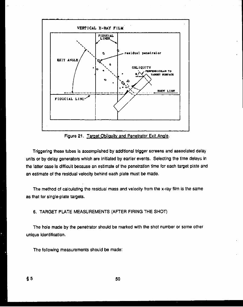
VERICAL X-RAY FILM

1IDUCIAL

LINES

%• 0 residual penetrator

EXIT ANGLE "LQI

NyPWDW1LIAN T

... .......... SH T / ,

FIDUCIAL LN:

Figure 21. Target Obliquity and Penetrator Exit Angle.

Triggering these tubes is accomplished by additional trigger screens and associated delay

units or by delay generators which are initiated by earlier events. Selecting the time delays in

the latter case Is difficult because an estimate of the penetration time for each target plate and

an estimate of the residual velocity behind each plate must be made.

The method of calculating the residual mass and velocity from the x-ray film is the same

as that for single-plate targets.

6. TARGET PLATE MEASUREMENTS (AFTER FIRING THE SHOT)

The hole made by the penetrator should be marked with the shot number or some other

unique identification.

The following measurements should be made:

§5 so

(1) Dittance from edge of entrwace to nearest target edge.(2) Front crater: width (diameter If normal impact); length (if oblique Impact).

(3) Entrance: width (diameter if normal Impact); length (if oblique impact).

Perforated Target

(4) Distance from edge of exit to nearest target edge.

(5) Exit: width (diameter if normal impact); length (if oblique Impact).

(6) Rear crater: width (diameter if normal impact); length (if oblique impact).

Nonperforated Target

(7) Normal depth of penetration.

(8) Une-of-sight depth (oblique impact).

(9) Height of rear bulge.

(These are explained in more detail in the remainder of this section.)

In addition, comments should be recorded concerning anything that is unusual.

6.1 Perforated Tarets.

6.1.1 Normal Impact.

- The shortest distance from the edge oi the hole to the nearest edge of the target for both

entrance and exit should be recorded. (This Is particularly important if the distance is less

than two projectile diameters because of the likelihood that the edge has influenced the

penetration process.)

* The length and width of the entrance hole and of the exit hole at the target surface

should be recorded (see Figure 22).

* Comments should be recorded concerning anything that is unusual.

51 §5

AT IMPACT SUEFACE RONT)

TARGET-CROSS SECTIoOr

-= [.(REAR)

_- L.... EXIT SURFACE

A - NEARMS EDGEC : CRATZR WVIDTH (MRM) I

L-EMTRANC"E VIANTrERD - EXIT DIAW-TERI1 CRATSR wIDTH (EXIT) E LI CU= RMINV - NEARIXT EDGE .SPALLED)

Figure 22. Perforated Target Measurements (Normal Impact).

6.1.2 Oblique Impact.

- The shortest distance from the edge of the hole to the nearest edge of the target for

both entrance and exit should be recorded. (This is particularly important if the distance is

less than two projectile diameters because of the likelihood that the edge has influenced the

penetraton process.)

* The length and width of the entrance hole and of the exit hole at the target surface

should be recorded (see Figur3 23).

- Comments should be recorded concerning anything that is unusual.

6.2 Semi-infinite and Nonperforated Targets. In order for a target to be considered semi-

Infinite, it must be of sufficient thickness so that shock waves reaching the rear surface do not

noticeably affect the penetration performance (the rear surface must not change shape). A

thickness which is twice the normal depth of penetration generally qualifies as semi-infinite.

§ 6 52

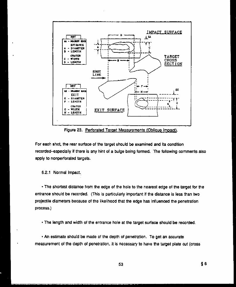
IMPACT-SURFACE

ID

LNRANCEA - DIAWIMr A ..C3- LENGTHi

CRAM TARGETC -WIIDTH ~ -- ~CROSSV ,LENGTH SECT ION

U Imac t=EXIT ------

E IAIMTERF LENGTHT

CRATER t0 WIDTH EXIT SURFACE -

H LENGTH

Figure 23. Perforated Tar-get Measurements (Oblique Impact).

For each shot, the rear surface of the target should be examined and Its conditionrecorded-especially If there is any hint of a bulge being formed. The following comments alsoapply to nonperf orated targets.

6.2.1 Normal Impact.

- The shortest distance from the edge of the hole to the nearest edge of the target for the

entrance should be recorded. (This is particularly important if the distance is less than two

projectile diameters because of the likelihood that the edge has Influenced the penetration

process.)

"• The length and width of the entrance hole at the target surface should be recorded.

"* An estimate should be made of the depth of penetration. To get an accurate

measurement of the depth of penetration, it is necessary to have the target plate cut (cross

53 §6

secton9cO) along the centerline of the hole since it Is likely that the residual penetrator is stuck

at the bottom of the hole.

- The rea; surface of the target should be examined for fracturo, bulge, etc.

Measurements should be made and noted.

* Comments should be recorded concerning anything that Is unusual (see Figure 24).

6.2.2 Oblique Impact

- The shortest distance from the edge of the hole to the nearest edge of the target for the

entrance should be recorded. (This is particularly important If the distance is less than two

projectile diameters because of the likelihood that the edge has influenced the penetration

process.)

• The length and width of the entrance hole at the target surface should be recorded.

• An estimate should be made of the depth of penetration. To get an accurate

measurement of the depth of penetration, it Is necessary tu have the target plate cut (cross

sectioned) along the centerline of the hole since it Is possible that the residual penetrator is

stuck at the bottom of the hole and because the hole can be measured by laying the ruler on

the cross-sectioned surface.

- The rear surface of the target should be examined for fracture, bulge, etc.

Measurements should be made and noted (see Figure 25).

- Comments should be recorded concerning anything that is unusual.

7. WITNESS PACK/PANEL MEASUREMENTS

Requirements for a particular firing program may include collecting Jnformation about the

behind-target fragment distribution with respect to mass and velocity. If all that is required in

regard to the behind-target fragments Is the distribution pattern and only rough estimates of

§6 54

I MPACTSURFACE TARGET CROSS SECTION

A B

u--- c -----c

A - NTAPZM Ma WHEN THE RES IDUAL PENITRATORA - CRATER WIDTH (OR LENGTH) REMAINS IN THE CAVITY, THMTARGET MUST BE Ctr. (CROSS-B - ENTRANCE DIAk•TER SECTIONED) IN ORDER TOC - DEPTH OF PENETRATION MEASURE THE DEPTH OF .ENE-

______________________ TRAT ION.

Figure 24. Semi-infinite Target Measurements (Nonr.al Impact.

.. - NU,•E SEDGEA c A - ENTRANCE WIDTH

- W - VNTRANCE LENGTH

IMPACT . C -. CRAT•. WID

SURFACE D - CRATER LENtTHI I E - LINE-OT-SICAHT

DEPTH! I F -NORMAL DEPFTH

SHOTL INE;

f

- I RES IDUAL PEMirRATOR

rr I' --

- �'TARGET"CROSS SECTION

r

Figure 25. Semi-infinite Target Measurements (Oblique Impact).

55 §6

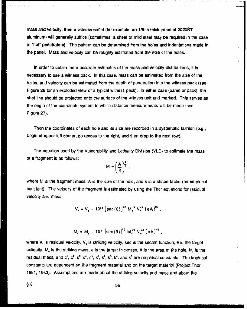
mass and velocity, then a witness panel (for example, an 1/8-in thick ranel of 2020ST

aluminum) will generally suffice (sometimes, a sheet of mild steel may DOe required In the case

of 'hot" penetrators). The pattern can be determined from the holes and indentations made In

the panel. Mass and velocity can be roughly estimated from the size of the holes.

In order to obtain more accurate estimates of the mass and velocity distributions, It Is

necessary to use a witness pack. In this case, mass can be estimated from the size of the

holes, and velocity can be estimated from the depth of penetration Into the witness pack (see

Figure 26 for an exploded view of a typical witness pack). In either case (panel or pack), the

shot line should be projected onto the surface of the witness unit and marked. This serves as

the origin of the coordinate system to which distance measurements will be made (see

Figure 27).

Then the coordinates of each hole and Its size are recordod in a systematic fashion (e.g.,

begin at upper left corner, go across to the right, and then drop to the next row).

The equation used by the Vuinerability and Lethality Division (VLD) to estimate the mass

of a fragment is as follows:

where M is the fragment mass, A is the size of the hole, and k is a shape factor (an empirical

constant). The velocity of the fragment is estimated by using the Thor equations for residual

velocity and mass.

Vr - V, - 1011 [sec(O)]C1 MC3 VC4 (eA)c,

M,= M, - 101, [sec(O)]12 M,'U V.14 (eA)S ,

where V, is residual velocity, V, is striking velocity, sec is the secant functiun, 0 is the target

obliquity, M, is the striking mass, e is the target thickness, A is the area o' tie hole, M, is the

residual mass, and c", c2, c3, c', c5, k', k2, k3, kV, and k' are empirical cocislants. The Impirical

constants are dependent on the fragment material and on the target materi'I (Project Thor

1961, 1963). Assumptions are made about the striking velocity and mass and about the

§ 6 56

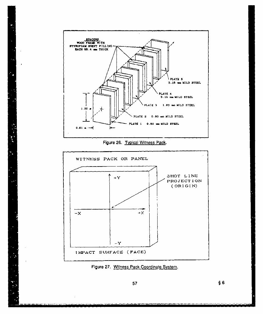
wooD irpl wiTH." i

sTYmrOOAw UHtT VIrLLtWO -EAC 26.4 wo THICK

SPLATE 5

-.18 me MILD STEEL

- 3.16 mo MILD STEEL

PLATE 3 1.60 mo MILD STEEL1.22•

PLATE 2 0.80 mu MILD STEEL

PLATE 1 0.80 mu W4ILD STEEL

Figure 26. Typical Witness Pack.

WITESS PACK OR PANEL

y .SHOT LINE

PROJECT ION( oR I G I N)

-x

IMPACT SURFACE (FACE)

Figure 27. Witness Pack Coordinate System.

57 §6

residual mass of the fragment. So, this methodology for estimating fragment mass and

velocity is very prono to error.

8. VELOCITY, THICKNESS, AND OBLIQUITY BALLISTIC LIMITS

8.1 Definitions, The most frequei t test of performance for a penetrator is comparing the

highest striking velocity which produces a penetration (sometimes referred to as a partial

penetration) or, alternatively, the lowest striking velocity which produces a perforation (not

necessarily the same value, but Is close) when fired against a specified target configuration.

This velocity is called the ballistic limit for that penetrator against that target. There are

several definitions for determining what qualifies as a penetration and a perforation

(Zukas et al. 1982). There is the Army criterion which defines a perforation to be any case

where any or all of the penetrator exits the rear surface; the protection criterion which requires

that a witness plate placed beh!nd the target be perforated to qualify as a perforation; and theNavy criterion which defines a perforation as any case in which light can be seen through the

hole (Figure 28).

The Army defines the value of the velocity ballistic limit to be the velocity at which there is

a 50% probability in perforating the target (V,,). The method of determining the V50 is

discussed in Section 8.2. Additional discussion of the velocity ballistic limit can be found in

Misey (1978).

Since vehicles are frequent targets for KE rounds and most vehicles present a variation in

target thickness and obliquity depending on the orientation of the vehicle in relation to a gun

system which is attacking, It Is of interest to determine at what obliquity a particular target

should be placed to just defeat the projectile. This value of obliquity is the obliquity ballistic

limit. Since the Greek letter theta (0) is frequently used to denote obliquity, the obliquity

ballistic iimit is often referred to as the "theta fifty" (the obliquity at which there is a 50%

chance of jett ing through, symbolically, 0.).

8.2 V., Method for Velocity Ballistic Limit. The V5 method establishes a striking velocity

which Is purported lo have a 50% probability of perforating the target. The most widely used

criterion i: -.alled the "six-round ballistic limit." Enough shots are fired so that there are three

§ 6 58

I

ARMY PROTECTI.ON ----- NAVY - _

PLATZ

PENETRATION (PARTIAL)

PERFORATION (COMPLETE PENETRATION)

Figure 28. Penetration (Partial) and Perforation Criteria,

penetrations (partials) and three perforations which all lie within a range of 125 ft/s (38 m/s).Then an arithmetic average (sum divided by the number of values) of these six values iscalculated, The resulting value Is the V6. The protection criterion for the result of a shot tobe called a perforation Is that a perforation be made by a fragment from the target or thepenetrator in a witness panel (usually 0.020-in Dural aluminum -4 2024ST aluminum) which isplaced 6 in behind the target.

An example of calculating the V,, is as follows. Assume the following set of experimental

data.

Striking (m/s) Result

1,523 Perforation

1,508 Penetration (partial)

1,533 Perforation

1,505 Perforation


1.507 Penetration (partial)

59 §8

The spread is 1,533-1,499 a 34 m/s (112 fps), so this set of values qualifies for a VW

calculation. The sum Is 9,075. Dividing by 6 yields an average value of 1,512.5 which would

be rounded off to 1,512. Therefore, the V. would be 1,512 m/s.

There are alternatives to the six-round limit velocity, if the number of projectiles is limited,

a two-round or four-round ballistic limit velocity may be reported. in some cases, It may be

necessary to Increase the range over which the velocities lie (e.g., 'I0-round ballistic limit

within 250 fps). In any case, the number of shots used in making the calculation should be an

even number, half of which are penetrations and the rest perforations. The ballistic limit

reported should idenilfy the number of shots and the velocity spread,

8.3 Method of Maximum Lifelihood. Golub and Grubbs (1956) describe a method of

,obtaining the most likely value for the intercept when the values involved occur in a zone of

mixed results (an overlap of successes and failures). In applying this method to evaluating

the ballistic limit velocity, two requirements must be met. First, there must be at least one

penetration (partial) that lies above the lowest perforation-the zone of mixed results.

Secondly, all the values to be used in calculating the ballistic limit must be close

together --that is, the zone of mixed results must be small.

The foliowing example reported in the article illustrates the method. Assume the following

set of data.

Velocity Condition of12 P§ Impact

2,453 Perforation


2,423 Perforation



In this set, a partial penetration (V = 2,433) occurs above a perforation (V = 2,423). This set

qualifies as a zone of mixed results. When firing at an impact velocity close to the limit

velocity, a number of factors can affect the outcome. For example, the partial might have

occurred because the yaw (or pitch) on impact was greater than for the perforation. The

§ 8 60

target or the penetrator might have had slightly different material properties which affected the

outcome.

The procedure to evaluate this set of data is as follows:

(1) Calculate the arithmetic average (denoted as ;p) as an initial estimate of the most likely

intercept value; g - (2,453 + 2,433 + 2,423 + 2,415 + 2,415)/5 = 12,139/5

= 2,427.8 fps.

(2) Calculate a sigma (a) on this estimate. This is done as follows:

- Sum the squares of the differences between each value and g..

(2,453 - 2,427.8)2 + (2,433 - 2,427.8)' + (2,423 - 2,427.8)' + (2,415 - 2,427.8), +

(2,415 - 2,427.8)2 w 1,012.8.

- Take the square root of the previous sum divided by the number of values.

012.8 14.23236.5

(3) Group the penetrations together separately from the perforations and calculate the

following quantities:

V____ t2__t ]penetrations 2,433 0.36536 0.13349 0.04877

(partials) 2,415 -0.89936 0.80885 -0.7274'

2,415 -0.89936 0.80885 -0.72745

perforations 2,453 1.77061 3.13506 5.55097

2,423 -0.33726 0.11375 -0.00384

61 §8

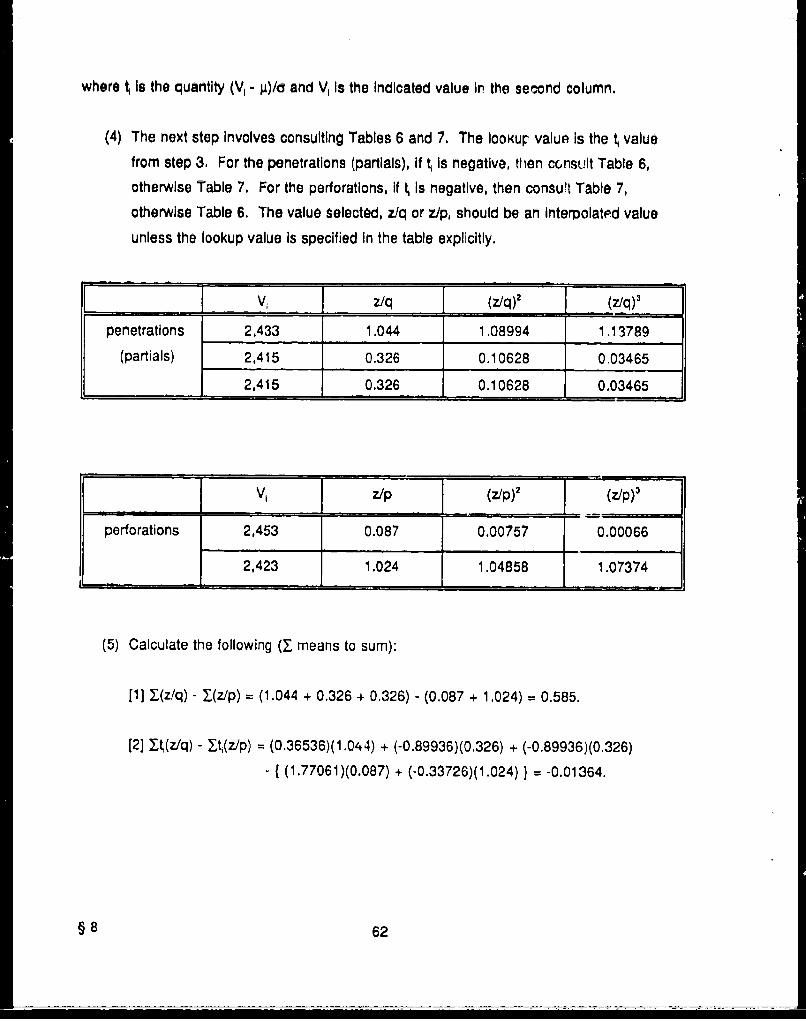
where t Is the quantity (V, - I)/c and V, Is the Indicated value in the second column.

(4) The next step Involves consutting Tables 6 and 7. The looKup value is the t value

from step 3. For the penetrations (partials), if tý Is negative, then ccnsulIt Table 6,

otherwise Table 7. For the perforations, If t Is negative, then consu!t Table 7,

otherwise Table 6. The value selected, z/q or z/p, should be an interpolatpd value

unless the lookup value Is specified In the table explicitly.

V, z/q (z-/q)2 (z/q)3

penetrations 2,433 1.044 1.08994 1.13789

(partials) 2,415 0.326 0.10628 0.03465

2,415 0.326 0.10628 0.03465

__________ ~J z/p (Zip)2 -J (Zip)3

perforations 2,453 0.087 0.00757 0.00066

-- J 2,423 1.024 1.04858 1.07374

(5) Calculate the following (X means to sum):

[1] Z_(zlq) - Y.(z/p) = (1.044 + 0.326 + 0.326) - (0,087 + 1.024) = 0.585.

[2] 2_,(z/q) - Yti(z/p) = (0.36536)(1.044) + (-0.89936)(0.326) + (-0.89936)(0.326)

- ( (1.77061)(0.087) + (-0.33726)(1.024) } =-0.01364.

§ 8 62

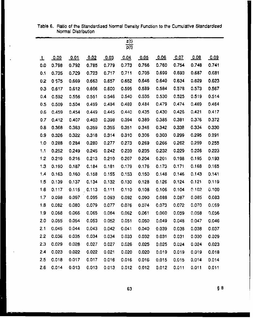
Table 6. Ratio of the Standardized Normal Density Function to the Cumulative StandardizedNormal Distribution

z(t)P(t)

t o.o oQ _ 0.01 0.02 0.03 0.04 0.05 ,06 0.07 0.08 0.09

0.0 0.798 0.792 0.785 0.779 0.773 0.766 0.760 0.754 0.748 0.741

0.1 0.735 0.729 0.723 0.717 0.711 0.705 0.699 0.693 0.687 0.681

0.2 0 575 0.669 0.663 0.657 0.652 0,646 0,640 0.634 0.629 0.623

0.3 0.617 0.612 0.606 0.600 0.595 0.589 0.584 0.578 0.573 0.567

0.4 0.592 0.556 0.551 0.546 0.540 0.535 0.530 0.525 0.519 0.514

0.5 0.509 0.504 0.499 0.494 0.489 0.484 0.479 0.474 0.469 0.464

0.6 0.459 0.454 0.449 0.445 0.440 0.435 0.430 0.426 0.421 0.417

0.7 0.412 0.407 0.403 0.398 0.394 0.389 0.385 0.381 0.376 0,372

0.8 0.368 0.363 0.359 0.355 0.351 0.346 0.342 0.338 0.334 0,330

0.9 0.326 0.322 0.318 0.314 0.310 0.306 0.303 0.299 0.295 0.291

1.0 0.288 0.284 0.280 0.277 0.273 0.269 0.266 0.262 0.259 0.255

1.1 0.252 0.249 0.245 0.242 0.239 0.235 0.232 0.229 0.226 0.223

1.2 0.219 0.216 0.213 0.210 0.207 0.204 0.201 0.198 0.195 0.193

1.3 0.190 0.187 0.184 0.181 0.179 0.176 0.173 0.171 0.168 0,165

1.4 0.163 0.160 0.158 0.155 0.153 0.150 0.148 0.146 0.143 0.141

1.5 0.139 0.137 0.134 0.132 0.130 0.128 0.126 0.124 0,121 0.119

1.6 0.117 0.115 0.113 0.111 0.110 0.108 0.106 0.104 0.102 0.100

1.7 0.098 0.097 0.095 0.093 0.092 0.090 0,088 0.087 0.085 0.083

1.8 0.082 0.080 0.079 0.077 0.076 0.074 0.073 0.072 0.070 0.069

1.9 0.068 0.066 0.065 0,064 0.062 0.061 0.060 0.059 0.058 0.056

2.0 0.055 0.054 0.053 0.052 0.051 0.050 0.049 0.048 0.047 0.046

2.1 0.045 0.044 0.043 0,042 0.041 0.040 0.039 0.038 0.038 0.037

2.2 0.036 0.035 0.034 0.034 0.033 0.032 0.031 0.031 0.030 0.029

2.3 0.029 0.028 0.027 0.027 0.026 0.025 0.025 0.024 0.024 0.023

2.4 0.023 0.022 0.022 0.021 0.020 0.020 0.019 0.019 0.019 0.018

2.5 0.018 0.017 0.017 0.016 0.016 0.016 0.015 0.015 0.014 0.014

2.6 0.014 0.013 0.013 0.013 0.012 0,012 0.012 0.011 0.011 0.011

63 § 8

Table 6. Ratio of the Standardized Normal Density Function to the Cumulative StandardizedNormal Distribution (Continued)

. 0.00 0Mo1L 0.02 0.03 0.0.L4 0.o05 0.6 ._7Z _08 2 0.09

2.7 0.010 0.010 0.010 0.010 0.009 0.009 0.009 0.009 0.008 0.008

2.8 0.008 0.008 0.008 0.007 0.007 0.007 0.007 0.007 0.006 0,006

2.9 0.006 0.006 0.006 0.005 0.005 0.005 0.005 0.005 0.005 0.005

3.0 0.004 0.004 0.004 0.004 0.004 0.004 0.004 0.004 0.003 0.003

3.1 0.003 0.003 0.003 0.003 0.003 0.003 0.003 0.003 0.003 0.002

3.2 0.002 0.002 0.002 0.002 0.002 0.002 0.002 0.002 0.002 0.002

3.3 0.002 0.002 0.002 0.002 0.002 0.001 0.001 0.001 0.001 0.001

3.4 0.001 0.001 0.001 0.001 0.001 0.001 0.001 0.001 0.001 0.001

3.5 0.001 0.001 0.001 0.001 0.001 0.001 0.001 0.001 0.001 0.001

3.6 0.001 0.001 0.001 0.001 0.001 0.001 0.000 0.000 0.000 0.000

1 exp - ;p(t) M- fz (t) dt,

Note: See text for conditions where this table is applicable.

Table 7. Ratio of the Standardized Normal Density Function of the Complimentary CumulatveStandardized Normal Distribution

z(t)

__t 0,00 0.01 0.02 0.03 0.04 0.05 0.06 0.07 0.08 0.09

0.0 0.798 0.804 0,811 0.817 0.824 0.830 0.836 0.843 j.849 0.856

0.1 0.803 0.869 0.876 0.882 0.889 0.896 0.902 G.909 0.916 0.923

0.2 0.929 0.936 0.?43 0.950 0.957 0.964 0.970 0.977 0.984 0.991

0.3 0.9.83 1.005 1.C.12 1.019 1.026 1.033 1.040 1.047 1.054 1.062

0.4 1.069 1.076 1.083 1.090 1.097 1.105 1.112 1.119 1.126 1.134

0.5 1.141 1.148 1.156 1.163 1.171 1.178 1.185 1.193 1.200 1.207

0.6 1.215 1.222 1.230 1.237 1.245 1.253 1.260 1.268 1.275 1.283

§ 8 64

M I I I I I I MI" I I I

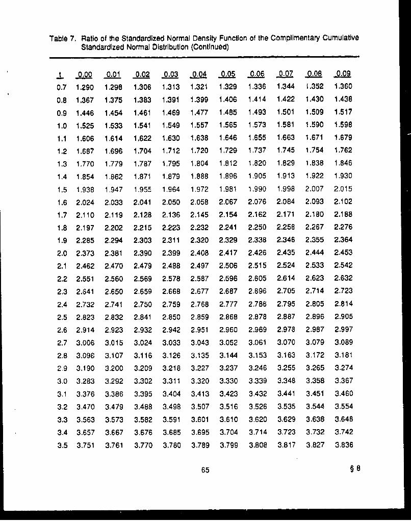
Table 7. Ratio of the Standardized Normal Density Function of the Complimentary CumulativeStandardized Normal Distribution (Continued)

t 0.00 0.01 0.02 0.03 0.04 0.05 0.06 0.09

0.7 1.290 1,298 1.306 1.313 1.321 1.329 1.336 1.344 1.352 1.360

0.8 1.367 1.375 1.383 1.391 1.399 1.406 1.414 1.422 1.430 1.438

0.9 1.446 1,454 1.461 1.469 1.477 1,485 1,493 1.501 1.509 1.517

1.0 1.525 1.533 1.541 1.549 1.557 1.565 1.573 1.581 1.590 1.598

1.1 1.606 1.614 1.622 1.630 1.638 1.646 1.655 1.663 1.671 1.679

1.2 1.687 1,696 1.704 1.712 1.720 1.729 1.737 1.745 1.754 1.762

1.3 1.770 1.779 1.787 1.795 1.804 1.812 1.820 1.829 1.838 1.846

1.4 1.854 1.862 1.871 1.879 1.888 1.896 1.905 1.913 1.922 1.930

1.5 1.938 1.947 1.955 1.964 1.972 1.981 1.990 1.998 2.007 2.015

1.6 2.024 2.033 2.041 2.050 2.058 2.067 2.076 2.084 2.093 2.102

1.7 2.110 2.119 2.128 2.136 2.145 2.154 2.162 2.171 2.180 2.188

1.8 2.197 2.202 2.215 2.223 2.232 2.241 2.250 2.258 2.267 2.276

1.9 2.285 2.294 2.303 2.311 2.320 2.329 2.338 2.346 2.355 2.364

2.0 2.373 2.381 2.390 2.399 2.408 2,417 2.426 2.435 2.444 2.453

2.1 2.462 2.470 2.479 2.488 2.497 2.506 2.515 2.524 2.533 2.542

2.2 2.551 2.560 2.569 2.578 2.587 2,596 2.605 2.614 2.623 2.632

2.3 2.641 2.650 2.659 2.668 2.677 2.687 2.696 2.705 2.714 2.723

2.4 2.732 2.741 2.750 2.759 2.768 2.777 2.786 2.795 2.805 2.814

2.5 2.823 2.832 2.841 2.850 2.859 2.868 2.878 2.887 2.896 2.905

2.6 2.914 2.923 2.932 2.942 2.951 2.960 2.969 2.978 2.987 2.997

2.7 3.006 3.015 3.024 3.033 3.043 3.052 3.061 3.070 3.079 3.089

2.8 3.098 3.107 3.116 3.126 3.135 3.144 3.153 3.163 3.172 3.181

2.9 3.190 3.200 3.209 3.218 3.227 3.237 3.246 3.255 3.265 3.274

3.0 3.283 3.292 3.302 3.311 3.320 3.330 3.339 3.348 3.358 3.367

3.1 3.376 3.386 3.395 3.404 3.413 3.423 3.432 3.441 3.451 3.460

3.2 3.470 3.479 3.488 3.498 3.507 3.516 3.526 3.535 3.544 3.554

3.3 3.563 3.573 3.582 3.591 3.601 3.610 3.620 3.629 3.638 3.648

3.4 3.657 3.667 3.676 3.685 3.695 3.704 3.714 3.723 3.732 3.742

3.5 3.751 3.761 3.770 3.780 3.789 3.799 3.808 3.817 3.827 3.836

65 §8

Table 7. Ratio of the Standardized Normal Density Function of the Complimentary CumulativeStandardized Normal Distribution (Continued)

t 0q.0 0.01 00.2 0 0.04 0.05 0.06 0.07 0.08 0.09

3.6 3.846 3.855 3.865 3.874 3.884 3.893 3.902 3.912 3.921 3.931

3.7 3.940 3.950 3.959 3.969 3.978 3.988 3.997 4.007 4.010 4.026

3,8 4.035 4.045 4.054 4.064 4.072 4.083 4.092 4.102 4.111 4.121

3.9 4.130 4.140 4.149 4.159 4.169 4.178 4.188 4.197 4.206 4.216

4.0 4.226 4.235 4.245 4.254 4.264 4.273 4.283 4.292 4.302 4.312

z(t) . '1 exp (- ;q (t)= 1-f z, (t)dt

Note: See text for conditions where this table is applicable.

Similarly, calculate the following:

[3] _t•(z/q) - X(z/q)2 - Yt,(z/p) - X(z/p)2 divided by 0.

[4] Xt 2(z/q)- YXt,(z/q)2 - E(z/q) - 2(z./p) - Zti(z/p)2 + X-(z/p) divided by a.

[5] t3 (z/q) - 2Y-t,(z/q) - Xt•2(z/q)2 - t,3(z/p) + 2,_t,(z/p) - _t2(z/p)2 divided by Y.

(6) The values computed in step (5) are used in the following set of simultaneous

equations to solve for changes to be made in the estimated values for ji and 0.

Steps (3) through this step are repeated using the revised values until the resulting

calculation of this step is within an acceptable tolerance value.

[1]= -([3] A + [4] A().

[2]= *-([4] Ag+[5]Aa).

§ 8 66

Here the bracketed values are replaced by the corresponding value calculated In step (5).

Then, AI. and Aa can be determined from the following symbolic equations:

[21[4] - [1][5][3] [5) - [4] [4)

* [2](3] - [1][4][4][4] - [3] [5]

The estimated intercept value (pi) and its corresponding cy is adjusted by adding the value for

Alg and Aa, respectively.

Newlt = old p +Ag.

Newc = old ao+a.

As Indicated previously, steps (3) through (6) are repeated until the value for AP. Is small

enough (less than 0.01, for example).

(7) The following table summarizes the values for the first four iterations. Since Al is less

than 0.01, the sequence is terminated.

'! [11] 121 (3] [4] 15] Al. •A

0.58065 -0.01331 -0.16674 -0.01213 -0.09126 3.560 -0.619

-0.03110 0.14215 -0.16436 0.06129 -0,14622 0.205 1.058

-0.00509 0.02336 -0. 15707 0.05304 -0.11325 0.044 0.227

-0.00018 0.00085 -0.15558 0.05151 -0.10716 0.002 0.009

The final P = 2,427.8 + 3.560 + 0.205 + 0.044 + 0.022 = 2,431.611, and•= 14.232

-0.619 + 1.058 + 0,227 + 0.009 = 14.097. Therefore, the ballistic limit velocity would be

67 § 8

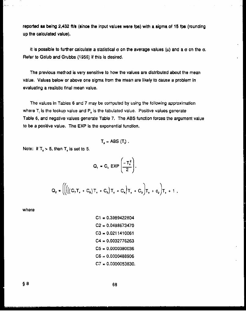
reported as being 2,432 ft/s (since the input values were fps) with a sigma of 15 fps (rounding

up the calculated value).

It is possible to further calculate a statistical a on the average values (L±) and a a on the a.

Refer to Golub and Grubbs (1956) if this is desired.

The previous method is very sensitive to how the values are distributed about the mean

value. Values below or above one sigma from the mean are likely to cause a problem In

evaluating a realistic final mean value.

The values In Tables 6 and 7 may be computed by using the following approximation

where T, is the lookup value and P. is the tabulated value. Positive values generate

Table 6, and negative values generate Table 7. The ABS function forces the argument value

to be a positive value. The EXP is the exponential function.

T, = ABS (Ta.

Note: If TX > 5, then T. Is set to 5.

0, - C1 EX 2T

02 - ((((CcT + CG)T., + ST + C.)T. + C 3}TZ + cj T, +1

where

C1 = 0.3989422804

C2 = 0.0498673470

C3 = 0.0211410061

C4 = 0.0032776263

C5 = 0.0000380036

C6 = 0.0000488906

C7 = 0.0000053830.

§8 68

If T, is positive, then 03 w 1 - I2028

If T, is negative, then 03

PX.~

03

The value of C1 is equal to L. The previous approximation is reported in Herr and

Grabarek (1978). Also refer to Golub and Grubbs (1950) and Hagan and Visnaw (1970) for

more information.

8.4 Lambert/Jonas Method for Velocity Ballistic Limit. Another method for caiculating the

velocity ballistic limit Is to fit the striking velocity and residual velocity data for a penetrator-

target configuration to the following equation:

v.. A (v3- (30)

where VR is the residual velocity, V, is the striking velocity, VL is the ballistic limit velocity (to

ba determined), and A and p are empirical constants (Lambert and Jonas 1976). The reason

for using this method for evaluating the ballistic limit Is that It generally reduces the number of

shots that need to be fired. For a six-round V5, a minimum of six shots has to be fired, of

which half must be perforations and the rest penetrations and all within a limited velocity

range. To achieve this when firing newly designed penetrators with only six shots would be

unusual. However, with only three shots which yield residual velocities, of which one Is less

than 500 m/s, a reasonably good prediction of the velocity ballistic limit can be made by fitting

to Equation 30.

In applying this equation to experimental data, A is restricted to the range 0 < A < 1, and p

is restricted to the range 1 < p : 8. The fit to the data is obtained by selecting a value for VL'

beginning with the lowest perforation and then allowing p to increment beginning at 1 and

stepping by 0.05. For each set of VL and p, A is determined by a least squares fit to the

69 § 8

perforation data. The value for VL is then decremented by ore until the set of values which

minimize the least squares error is found. The least squares fitting procedure is terminated

prematurely if the selected value for VL has been decremented down to the high6st

penetration.

This method for evaluating the balilstic limit does not require any penetiation data

(partials). The equation !s too sensitive to the convergence point to permit using a nonlinear

least squares technique to obtain a solution.

It only one perforation point is available, then the value I is assigned to A and, areasonable value 'or p is selected based on any data sets for the same penetrator and target

obliquity, which are more complete.

A method for estimating the values for A, p, and VL apriori Is given in Lambert (1978).

This method is the following. Setting z - .T [sec (9)]. ', where T is the target thickness,

D is the penetrator diameter, 0 is the target obliquity, and sec is the secant function, the value

for A can be estimated from the following:

A = _ M where M' 1ýM/ P (31)

M + 4 3

3

M is the penetrator mass, and p, = 7.85 (value used in report i. 7.8). Note that M' is related

to the mass of a plug of the target plate with the same cross-sectional area as the penetrator.

The value for p may be estimated from p = 2 + z. This equation is probably not applicable3in general because it is possible to get unrealistically large values for thick targets.

Finally, the ballistic limit velocity for RHA targets may be estimated from the following:

VL - 4,000 L '[z + EXP (-z) - 1] D•3

§8 70

where EXP is the exponential function and L, D, and T are in centimeters, M i; grams, and VL

in rn/s. A discussion of the rationale behind these equations Is given ir, Zukas et at. (1982).

8.5 Thickness Ballistic Limit. In experimental work, a firing program will generally call for

obtaining a velocity ballistic limit for a particular target c,'infigurafiorl. However, It is also

possible to have a particular striking velocity specified (for example, the expected velocity at a

specified distance from a particular gun) and then ask what thickness of target is required to

just stop the penetrator. Since plates used for targets are available onl%, in discrete

thicknesses, it is not feasible to obtain a thickness ballistic limit directly through experiment. A

good estimate can be made graphically if velocity ballistic limits both above and below the

specified striking velocity are available.

8.6 Obliouity Ballistic Limit 0ON. The 0e is determinod in a manner similar to the V5,

exceot that the striking velocity is held constant (as near as possible) and the obliquity is

vat, - , round the value at which the penetrator will just perforate the target. A standard

definition of the number of shots needed for a 0. doesn't exist. An acceptable condition

would be three penetrations and three perforations within a 100 spread in obliquity and with

the striking velocity within 25 m/s. In any case, the criteria used should be reported so that at

some fuiure time, verification can be made if necessary. Refer to Figure 29, which shows that

the 6C, lies between 02 where perforation occurs and 0, where only penetration occurs and

that 0, > 02.

9. PENETRATION/PERFORATION EQUATIONS AND THEORY

9.1 Sy•.bols. The equations described in this section will use symbols to represent

parameters which are defined as in the following.

A - empirical constant, or area

B - empirical constant, or area

C - empirical constant, or area

D - penetrator diameter

E - Young's modulus

F - force

71 §8

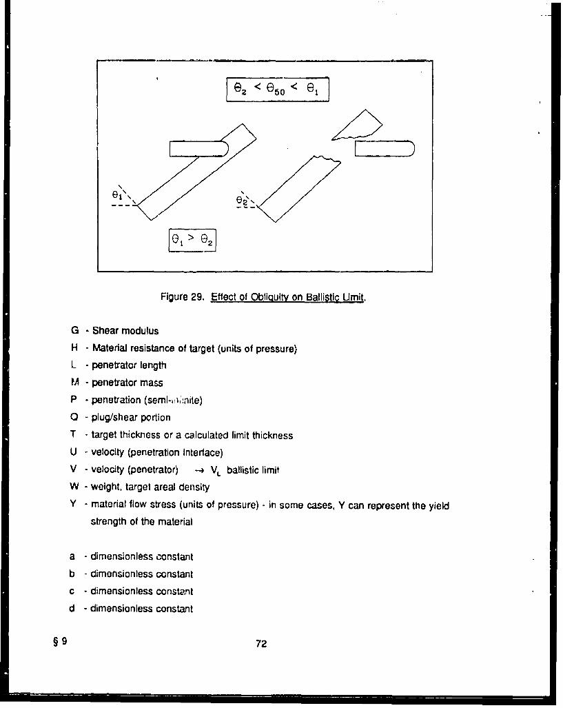
Figure 29. Effect of Obliqulty on Ballistic Umit.

G - Shear modulus

H - Material resistance of target (units of pressure)

L - penetrator length

M - penetrator mass

P - penetration (semi-,•:nite)

Q - plug/shear portion

T - target thickness or a calculated limit thickness

U - velocity (penetration interface)

V - velocity (penetrator) -4 VL ballistic limit

W - weight, target areal density

Y - material flow stress (units of pressure) - in some cases, Y can represent the yield

strength of the material

a - dimensionless constant

b - dimensionless constant

c - dimensionless constant

d - dimensionless constant

§ 9 72

a - dimensionless Constant

f length/diameter ratio (fineness ratio)

g - a Grabarek's constant

h normalized crater/hole cross section

k - dimensionless constant

I P

mn

t -time

u - Instantaneous velocity

v Instantaneous velocity

w - instantaneous velocity

The following, when used as subscripts, will have the indicated meaning.

L - limit

p - parameter related to the penetrator

r,R- residual

s,S- striking

t - parameter related to the target

0 - initial value

50 - probability is 50%

Characters from the Greek alphabet have the following meanings.

alpha (a) - empirical constant or angle

beta (P3) - empirical constant or angle

theta (0) - angle of obliquity

pi (n) - ratio of circle circumf&rence to diameter (3.141592654...)

rho (p) - matodal density

73 §9

I I I I I I I I I-

9.2 Enaineerina Models.

9.2.1 Purely Empirical Equations. Numerous empirical (constants evaluated from

experimental data) equations have been used to describe penetrator performance for KEprojectiles. Some equations are purely empirical and are quite limited in making predictions,

while others are based on physics principles. The latter are more likely to give good

predictions, but the ultimate equation, which is applicable in all cases, has not been found,

An example of the purely empirical equations are the well known THOR equations describedIn Project THOR (1961, 1963) and Johnson and Mioduski (1966). These equations have the

following form:

VR = Vs - A (TAn)" Mb V [sec(O)]d , (32)

where V. is the residual velocity, Vs is the striking velocity, T is the target thickness, AP, is the

penetrator cross-sectional area, M is the penetrator mass, sec Is the secant func,.n, 0 is the

target obliquity, and A, a, b, c, and d are empirical constants; and- )l M I V "' e 0 ] n

MR =Ms- B (TA) M [sec(0)], (33)

where MK is the residual velocity, M. is the striking mass, and B, k, I, m, and n are empiricalconstants. The values of the empirical constants are highly dependent on the set of data

used to evaluate the constants. Therefore, predictions of events involving conditions which lie

outside the set of data are not reliable. The values of the empirical constants are alsodependent on the units used for the parameters. A modification of Equation 32 is described in

Zook, Slack, and lzdebski (1983), which equates the loss of KE (assuming no loss in mass) tothe second term of the right side of Equation 32. This equation is as follows:

1 M, (V2 - V') = KT- Apb M I V 4 [sec(o)]. (34)

This equation gives tho curvature in the V. - V. curve that is observed in most experimental

data as the residual velocity approaches 0.

§9 74

Another empirical approach to penetration performance Is described In Appendix E of

Lambert (1978).

The method described in the report for estimating the values for A, p, and VL in the

equation

v-W A (v P- VL)1

Is as follows. Set

T

where T Is the target thickness, D is the penetrator diameter, 6 is the target obliquity, and sec

is the secant function. The value for A can be estimated from the following:

A ,, M where Mj PD 3 zMA + M/ 4

3

M Is the penetrator mass, and Pt = 7.85 (value used In report Is 7.8). Note that M' is related

to the mass of a plug of the target plate with the same cross-sectional area as the penetrator.

The value for p may be estimated from the following:

p -2 +. .

3

This equation is probably not applicable in general because it is possible to get unrealistically

large values for thick targets.

Finally, the ballistic limit velocity for RHA targets may be estimated from the following:

VL -4,000 L [z + EXP(-z) - M] D 3

75 §9

where EXP Is the exponential function and L, D, and T are in centimeters, M in grams, and VL

in m/s. A discussion of the rationale behind these equations Is given In Zukas et al. (1982).

9.2.2 Semlempirical Equations. A step above purely empirical equations is relating

nondimensional quantities (Baker, Westine, and Dodge 1973). Ratios are formed based on

the parameters Involved in such a way that the numerator has the same units as the

denominator, and, therefore, the ratios are dimensionless. Such ratios are as follows:

L penetrator lengthD penetrator diameter

T target thicknessD penetrator diameter

Pp pernetrator density

pt target density

and

1 V2

2 PP penetrator KE per unit volumeH target resistance

The first equation of Grabarek's equations (to be covered more fully in Section 9.2.5) is based

on a relationship of three of the prevk,.,s ratios-the first, second, and last.

pp D [(35)

H LD

By letting 1 H n - A and p L = M, Equation 35 becomes2 4

§9 76

VL A [saco) (36)

which is Grabarek's single-plate equation.

Most penetration equations which have some physical basis may similarly be reduced to a

relationship of dimensionless ratios. For example, the equation reported in Zook (1977) is

derived from an expression for the resistive force experienced by the penetrator. In compact

form, this equation is as follows:

T - 4M f(VS, VRH, p) . (37)7t D 2 p,

This equation does not consider oblique impacts. The expression for the function

f(V8, VM, H. p) Is made up of quantities which are dimensionless ratios and, therefore, the

function Is dimensionless. For a right circular cylinder, Equation 37 may be rearranged to the

following:

T .[L PP)f(Vs, V,,H, p,), (38)

by substituting pp L ... Z for M and dividing both sides by D.4

One word of caution when applying the equation in MR 2797 to new data--that equation

works well only for penetrators which have an L/D ratio of nearly 1 (as in the report). For

penetrators with L/D ratios greater than 1, a different expression, which includes the length

parameter, must be used for the force equation unless the penetrator strength exceeds that of

the target and the penetrator does not lose mass as a result of the interaction. A satisfactory

force equation which can be integrated and is applicable to penetrators with high UID ratios

which erode during the penetration process has not yet been found. However, a penetration

model which can be applied to both eroding and noneroding penetrators will be described in

Section 9.2.4.

77 § 9

9.2.3 Semltheoretlcal Equations. Some of the penetration equations have a physlcal

rationale. The usual starting point Is to define an expression for the resistive force acting on

the penetrator by the target, The simplest assume the resistive force to be a constant as

follows (proposed by Robinson (circa 17421 and Euler [circa 1750]):

F = A. (39)

From physics, the force is equal to the mass multiplied by the acceleration. In this case, the

penetrator Is being decelerated (minus sign). Therefore,

F = -Ma = A. (40)

From calculus, the acceleration a can be expressed as dv/dt or as (dv/dx)(dx/dt) which is

equal to v (dv/dx). Therefore,

-Mv dV .A. (41)dx

Integrating this expression with the limits v = Vo when x = 0 and v = 0 when x = P and

assuming M and D to be constant, yields the following relationship:

SiVo2 AAP. (42)2

The left-hand side of this equation is the KE of the penetrator on impact. The right-hand side

is proportional to th3 volume of the crater made in the target (set A = A, H, where Ah, is an

average hole cross-sectional area and H is the target resistance). The concept of volume of

the crater being proportional to the work done in creating the crater has been attributed to

Morin (1833) and to Martel (1897).

More complicated expressions for the force equation have been proposed.

F =A + BV , (43)

§ 9 78

F A + BV9 (Poncelet [circa 1830]), (44)

F BV + CV2 (Resai [circa 1895]), (45)

and

F-A + BV + CV'. (46)

The previous equations are expressed without the cross-sectional area, AP, as part of the

equation. However, it is known that the resistive force is a function of the cross-sectional

area. When AP is treated as a constant, the result will represent an average force. The

aerodynamic force acting on a projectile in air is known to have the following form:

F -1 CdAPp(0) V2 (47)2

where C3, is the drag coefficient and P(,s is the density of air. The drag coefficient is not

constant but varies with the velocity of the projectile. However, for velocities below the speed

of sound in air (approximately 1,100 fps), known as Mach 1, the drag coefficient is nearly

constant Above about Mach 1.5 (one and a half times the speed of sound in air), the drag

coefficient decreases almost linearly with increasing speed. See Figure 30 for typical drag

coefficient curves.

Integration of the aerodynamic force equation with respect to range yields the following

equation, assuming Cd to be constant:

V=Vo exp -Cd AP2MP(.) Rj, (48)

where V. is the velocity at the range R = 0 and exp is the exponential function. For a given

value of R, the resulting velocity may be calculated. The result is NOT valid for velocities

above Mach 0.8, except that above Mach 1.5; Cd may be considered constant only over small

changes in speed. If R is in meters, then M must be in kilograms, AP in square meters, and

p.,; in kilograms per cubic meter. The density of air under standard conditions (sea level, no

79 §9

1.2 t---- . . .-.. . . I -,- , -:. . . .

MACH I IS TIE SPEED OP SOUND IN AIR

.4

0

0ARMY PROJECTILES

0 4 6 8 10MACH NUMBER

Figure 30. Typical Drag Coefficient Curves.

humidity, and 700 F) Is apprcximately 1.229 kg/m 3 (Johnson 1972; Backman and Goldsmith

1978).

9.2.4 A Finite Thickness Target Model. Recent analysis of perforation performance

indicates that perforation involves two stages-a penetration phase in which the action taking

place is the same as if the target were semi-infinite and a breakout phase in which the

expended energy is directed toward fracturing the bulge which forms on the rear surface and

accelerating the target material (plug) which breaks free. For long rod penetrators, the depth

of penetration is proportional to the length of the penetrator multiplied by the striking velocity

raised to a power. The thickness related to the breakout phase is proportional to the diameter

of the penetrator. This is represented by the following equation:

T -Lcos(O)L +AD , (49)

where 0 is the angle of obliquity, VL is the ballistic limit for thickness T, and A. B, and C are

empirical constants evaluated by fitting at least three velocity ballistic limit values, and cos is

§9 80

the trigonometric cosine function. When fitting ballistic limit data resulting from more than one

penetrator, a better fit for RHA targets might be obtained by modifying the equation to the

following:

T - 5 cos() . +AD . (50)

Values for A range generally from -1 to 2; for B, the range of values is from 1.5 to 3; and for

C, the range of values Is from 1,000 to 3,000 when T, L, and D are in millimeters and VL is in

meters per second. No method has been found yet to calculate values apriori for A, B, and C,

so a fit must be made to experimental data. However, after finding A, B, and C for a

particular penetrator vs. target material, reliable estimates of ballistic limits may be made for

other thicknesses and obliquities.

9.2.5 Grabarek's Equations. After establishing the ballistic limit (VL values for several

target thickness/obliquity configurations, a fit may be made to determine the empirical

constants in Equation 51. This equation will permit predictions of the ballistic limit for other

target configurations. The values of the empirical constants are dependent on the target

material and on all characteristics of the penetrator.

VL D [ M- (51)

where VL is the ballistic limit (meters/second), A Is an empirical constant, D is the penetrator

diameter (mm), M is the penotrator mass (grams), T is the target thickness (mm), 6 is the

target obliquity, sec is the secant function, and a and P are empirical constants. The values

for A range from about 5,000 to 60,000 or more, depending on the material properties of the

penetrator and the target Values for a and 03 are usually close to 1. If 5 is less th3n 1, then

the penetrator performs better when fired against an oblique target than would be expected

based on line-of-sight thickness (compared to normal impact).

81 §9

The form of Equation 51 has been reported in Grabarek (1971, 1976) and Herr and

Grabarek (1976).

To predict the residual velocity (VA) for a given striking velocity (V,) where the ballistic limit

is known, the following may be used:

VR V aX2 + bX + CF,/-(52)VR -V (52)

where X -_ Vs - 1 , a = 1.1, b = 0.8, and c = 1.65. If the striking velocity Is greater than eightVL

times the limit velocity, then the residual velocity is approximately 99% of the striking velocity.The values given for a, b, and c can be used in general. However, as empirical constants,

the values are dependent on the penetrator and the target. This equation Is reported In Herr

and Grabarek (1976).

The residual mass (MR may be estimated using the following equation:

MR - MB [X ( D• )I -1 ksec (e) (53)

where B and g are empirical constants, X is that of Equation 52, k is thb projectile material

factor (a value of 1 may be used, although a value greater than I should be used for high-

density materials), D Is the penetrator diameter, and L is the penetrator length. If the

calculation for MR is negative, then the residual mass is assumed to be 12% of the striking

mass. Typical values for B lie in the range of 0.3 to 0.8 and for g, In the range 0.1 to 1.

These three equations may be used to make predictions about penetrator performance

when fired against multiple-plate targets. The residual velocity and residual mass become the

striking velocity and striking mass for the subsequent plate. Complications due to systematic

deflection or misorientation of the penetrator while perforating the target array are not explicitly

accounted for. Reasonably good fits to experimental data can be made over only a modest

range of velocities and obliquities.

§ 9 82

9.3 Theoretical Models.

9.3.1 The AXekseevskii/Tate Penetration Algorithm.

The Equations. A frequently used algorithm for making quick (compared to

hydrocodes), approximate predictions of long rod penetration performance impacting

semi-infinite targets is that proposed by Alekseevskli (1966) and Independently by Tate

(1967, 1969). The justification for the first two of the four basic equations Is shown in

Figure 31. In these equations, L is the Instantaneous length of the penetrator, V Is the

velocity of the tail end of the penetrator, U is the axial velocity at the interface between

the penetrator and the target. and P Is the instantaneous depth of penetration.

The erosion rate of the penetrator is as follows:

AL, -(V - U). (54)

At

The minus sign Is due to the fact that the erosion rate is decremental. The material which is

eroded makes no direct contribution to the penetration.

The penetration rate is A'P U (55),&,t

A schematic representation of the conditior;t, for the third and fourth equation is shown in

Figure 32.

The force balance at the base of the pene'rator head region when Y < H or when Y > H

and U < V is as follows:

AP Lpp AV AP Y . (56)At

83 § 9

GIVEN A TIME INCREMENT eAL

DISTANCE TRAVELLED WITH NO TARGET

LENGTH ERODED DISTANCE TR~AVELLED IN TARGET

(V-U) & t U At

THEREiFORE: k v-U) and A

Figure 31. Basis for Ecluations 5". and 55.

TARGET "tMFACE

IRIGID PORTION Or PNTAO ARE mrC

PENKTRATO OftG IH EOCT

(of Ieogth L)TRtAVELLING AT

VELOCITY V

I XAT IN~SR AAC TPrERTR:RrTERFACE

(AVERAGED OVER PEN ETRATOR CPS-ECINLATRES)

P dt. Y + kpf, ( V - U) 2 = H +ktFt U2

Figure 32. Schematic Illustrating Ecuations 56 and 58.

§9 84

Ap is the initial penetrator cross-sectional area, and p, Is the penetrator density. When the

pressure between the rigid portion of the penetrator and the target Interface no longer

supports material flow, then the remaining penetrator becomes rigid. Under these conditions,

APLp AV. -A+(H + k P, , (57)

or, equivalently, Y = H + kp2V2. In this case, Y is no longer Interpreted as flow stress but as

the resistive force of the target; KI is a factor related to the target, and p, is the target

density.

The fourth and last of the basic equations is the modified Bernoulli equation, which is the

pressure balance across the penetrator-target interface while the penetrator is eroding, and is

as follows:

Y + k, pp (V - U)2 w H + kp,U2 . (58)

Equations 56 and 58 are based on the following simplifying assumptions.

(1) The dynamic behavior of the homogeneous penetrator is that of a rigid body up to

some pressure Y (the flow stress of the penetrator). Likewise, the homogeneous

target acts as a rigid body up to some pressure H (the target resistance). The

penetrator material flows like a fluid for pressures at or above Y, and, likewise, the

target material flows like a fluid for pressures at or above H.

(2) The retardation of the rigid polion of the long rod penetrator of length L is determined

only by the pressure Y, which is the maximum stress level the still rigid rod material

can sustain before it begns to act as a fluid.

(3) After an initial impact transient, the penetrator-target interface moves with a velocity U.

If the penetrator erodes (becomes shorter than the initial length Lo while penetrating

the target), the rigid portion of the penetrator has a velocity V. while the front end

85 § 9

travels with the velocity U. Relative to the penetrator-target Interface, the penetrator

travels with a velocity V - U.

These four equations model the penetration process quite well for the time between the

end of the Initial impact transient (on the order of microseconds for metallic interactions) and

the time when the penetrator erodes down to the length of the head region-generally

between one radius and one diameter. For long rods, most of the penetration occurs between

the two end phases and, therefore, the model is reasonably accurate in predicting depth of

penetration. For short rods, most of the time is spent In the final phase, and the basic four-

equation model underpredicts the depth of penetration.

The Alekseevskii formulation treats k, and kP as shape factors. Tate takes the values for

kP and k1 to both be 1/2, corresponding to the values which appear in the original Bernoulli

equation (what follows Is based on k. k = 1/2). Equation 58 is a quadratic equation In U

and can be solved as follows:

L. LL, a= 1 -I,b -2V, and c = V2 , - HkP pp kP pp

then, if a = 0, then U C- _ . (59)

Otherwise, the discriminant d - b2 - 4ac must be evaluated.

Ifd_>0, then U = -b - . (If d =0, p. must not be 1.) (60)2a

If d < 0, then Ys H, then U = 0; otherwise, U = V. (61)

The interface velocity U has the restriction 0 5 U <_ V, and a check must be made to assure

that it does not fall outside that range. The upper limit on th, ,,•ue of V when I) r,"lrhes a

§ 9 86

limit on its range can be calculated. When H ! Y and V -Y, then U = 0 (noko pp

penetration occurs, but the projectile continues to erode until V -ý 0). When H < Y and

V < IZ'-Hthen U = V (the penetrator behaves as a rigid body). When V is greater thanSk, Pt

either critical value (depends on relation of H to Y), then both erosion and penetration will

occur,

Figures 33 through 35 Illustrate the behavior of Equation 58. These figures show the

effect of varying Y with respect to H (H remains constant) for three different penetrator

densities. In Figure 34, the penetrator and target have the same density. The curve labelled

2 in each of these figures is for Y = H. The value of U is the rate at which penetration occurs.

The conclusion may be drawn that if Y 5 H, the penetrator will always erode (because

U < V), and if Y < H, there exists a positive value of V where U will go to 0 as explained

previously. Below this value of V, no penetration into the target occurs. However, the

penetrator continues to erode until V goes to 0. On the other hand, If Y -- H, there exists a

value of V below which the entire penetrator Is rigid (U = V). Above this value of V, the

penetrator erodes.

If Equations 59, 60, and 61 are approximaLed by U V + anP

V 1 + IL k-ýP-PH-Y and if Y and H are assumed to be constants, then these equations can be

kP pPintegrated in closed form for the cases where Y = 0, Y = H, and Y = H/(2 + 4). These are the

S1, S,, and S3 functions which have been published in Frank and Zook (1987, 1991).

If Equation 54 is set to 0, representing a constant mass (rigid) penetrator (requires

Y > H), then Equation 57 is applicable and can be integrated in closed form to yield the

following:

In Hf1 (62)L0 2k, o ,

87 §9

b~xh~u11i Equation behiaviour *Cam* 12500 - ----- -.--- ,-

y khop ko wi Ahot kt

1 2 .0 2177 a 0I35 5.0 743c a.1

2000 2 6. 371) 0.()5 1 .0 V550 0.1 6

1800.

U 10 0

5001

0 1000 2000 3000 400000 50

V ( M / 0) - -

Figure 33. U vs. V for Y =2, 5, and 8 GPa and o., = 2,770 k /rn'.

Bernoulli Equation Behaviour Came 23500 - - t II

POF k U- / nIOPa kQ/=u3

300- .0 7050 0.9 9.0 7550 0.53 5.0 7350 0.0 S.0 7650 0.3

3300

2000

1500

1000

500

0

0 1000 2000 3000 4000 5000 5500

V (r/'

Figure 34. U vs. V for Y = 2, 5, and 8 GPa and pp 7,850 kg/rn3.

§9 88

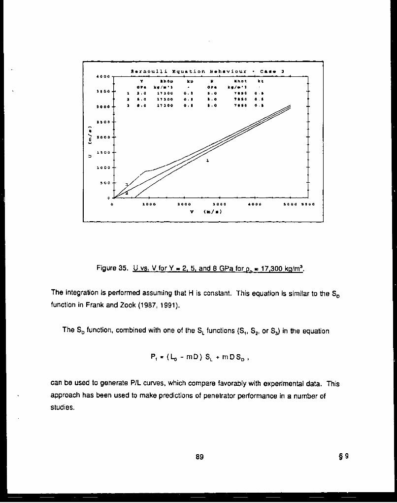
Sernoul1i Rquation Sithaviour *came 3

Y R340 kv V MKhot ktor& kg/M1 drd kg/013

L0 2. 20 11300 0. 5 a 0 V7a3S0 0.5

a 1.0 172300 0 . 1 a.0 iota 0.a

loo 3*0 100 0. ao S~o cm 7650 0 1

2500-

b1500 }1000

Soo

0

0 1000 1000 3000 46000 5000 S500

V (in /

Figure 35. U vs. V for Y = 2. 5, and 8 GPa for ~r, = 17300-ka/rn

The Integration Is performed assuming that H is constant. This equation is similar to the SD

function in Frank and Zook (1987, 1991).

The SD function, combined with one of the SL functions (S,, S2, or S3) in the equation

Pf -(LOa - mD) SL + m D SDI

can be used to generate P/L curves, which compare favorably with experimental data. Thisapproach has been used to make predictions of penetrator performance in a number ofstudies.

89 § 9

- Datermining a Value for Y From Experiment. Y Is Identified as being the pressure at

which the material begins to flow (deform plastically). The value of Y can be determined from

low strking velocity experimental data. When a penetrator impacts a target which has greater

strength than the penetrator at low speeds (below about 500 rn/s for tungsten alloy or DU vs.

RHA), the penetrator erodes and any penetration into the target is a few millimeters at most.

So the assumption Is made that U = 0. Equations 54 and 56 with U = 0 are solved

simultaneously for Y and integrated to produce the following:

I 2

Y , (63)

In Lo

where L, is the measured residual length and LI Is the Initial length. It is necessary to recover

the residual penetrator In order to obtain L,, since it would be difficult to estimate a proper

delay time to catch the residual penetrator on x-ray film. Since little or no penetration of the

target occurs, the penetrator remains at the target surface until V -. 0.

Figures 36 and 37 show the variation of Y for some penetrator materials. Figure 36 is

based on data reported in Wilkins and Guinan (1973). From Figures 36 and 37, it appears

that Y may be a function of the striking velocity. However, there was some penetration (less

than 8 mm) for the data of Figure 37 and part, if not all, of the variation of Y is not rea;

(Equation 63 assumes 0 penetration). The amount of penetration for the data of Figure 36

was not reported. Since Y is assumed to be constant, the value to be used is the

extrapolated value at V = 0.

Equations for computing Y, which are slightly more complex than Equation 63, have been

proposed. The first is Taylor (1948). Wilkins and Guinan (1973) offer a similar equation. The

added complexity of these equations does not seem to be justified.

§ 9 90

Wilkin,, & auinan, Y. Appl. Phys., War 10!31 .7090 #tool L/- 3--4

* •2 "69 *k*l*1 ",/P 2 -

v~ TI eat. Io ./ 3.a.. vsa~nitaa bi.' sa 2& .0.-*- pm U Yi1LuM all.y L/b 3

@A 7 A dOdiYC &IM. L/O P .6" /Y a6 a c•. otp L/D I

v-- MaagAseUe, allay L/D 3-1

2 ' Ob l,/,o DJhed 1L.hoe g*Pz***lnt

rite to ga~te or• soerage.A.

aa.

A- A ---- A2.

.4/4

0. A. J(Lo/L 6f

-- -I

0 .2 .4 ,4 ,8

X14PACT VELOCITY (km/s)

Figure 36. Material Flow Stress Y for Various Materials.

"RIcIn, TARGET p < mm3 I - -

3.5a --

C6

------------ --J-----

02 K 2 A./D 1

a1.2

(• x .- '-;17 WA i/O-b0

SX - 1-27 WA i/b-is

o pv,/2 K -I WA- L-/0-1

•' s • (•o Lc)U - 0u-3/4Ti -/b-1

b..kod i~n.. *.e ... eot; 6t.• to d~lt*

0 I I ' I

0 ,3 .4 .6 ,.6

IMPACT VELOCITY (km/b)

Figure 37. Material Flow Stress Y for Tungsten Alloy and DU.

91 §9

, Daterminlng a Value for H. The target resistance pressure H deep in the target can be

determined from cavitation analysis (Hill 1950; Hopkins 1960; Goodier 1965; Hanaeud and

Ross 1971; Tate 1986a).

Expanding cylindrical cavity (Hill 1950),

H la [1 + In L + •Et (64)

Expanding spherical cavity

(Hopkins 1960; Goodier 1965)

2Y F 2El 2n~2H ...... 1 + In _Y +T Et. (65)3 L

Expanding spherical cavity (Hanagud and Ross 1971),

H W - 1Y S - -- + In 2E + - c Et. (66)3 E 27

Advancing cavity (Tate 1986a)

H = YVS [2~ + in 2E (67)

In these equations, Yy, is the target yield strength (identified as Y in Figure 38, E is

Young's modulus, and E, is the slope of the curve from the yield point to the ui;mate strength

point (assumes a bilinear stress-strain curve). Tables 8 and 9 show relevant material

§ 9 92

BI-LINEAR STRESS STRAIN

STRESSiý

Y- SLOPE - Et

SLOPE E E

00 STRAIN

,igure 38. Bilincar Streso-Strain Slope Definitions.

Table 8. .. ,e 46cd Material Properties

Material Density Yield E '

(kg/m 3) (GPa) (GPa) (GPa)

RHA 0.5" 7,850 1.23 208 0.64

RHA 1.5" 7,850 0.87 206 0.76

RHA 4.0" 7,850 0.94 206 0.44

HHA (USSL) 7,850 1.72 214 2.38

Al 70 9 2,800 0.41 75 0.55

WA 90% 17,200 1.18 324 2.56

93 § 9

Table 9. Computed Values of Target Resistance

Material HiH 2 H, H4

(GPa) (GPa) (GPa) (GPa)

RHA 0.5" 4.31 5.16 5.16 6.63

RHA 1.5" 3.39 4.07 4.07 4.98

RHA 4.0" 3.41 4.07 4.07 5.31

HHA (USS,L) 6.54 7.95 7.94 8.75

Al 7039 1.64 1.99 1.99 2.24

WA 90% 5.54 6.76 6.75 6.93

H, - Equation 64 (Hill 1950).

H2 - Equation 65 (Hopkins 1960; Goodior 1965).

H, - Equation 66 (Hanagud and Ross 1971).

H4 - Equation 67 (Tate 1986b).

parameters and the resulting calculations for H. The yield, E, and E, in the table were

obtained from bilinear approximations to stress-strain compression tests performed at the

BRL

The values in Table 9 are the values for H using the values of Table 8 in Equations 64

through 67.

The values for H, (the last column) are in close agreement with the values needed in the

algorithm to give reasonable agreement with experimental data in the ordnance velocity range

(1,000-1,800 m/s).

An alternative method for calculating H based on the BHN and Young's modulus is given

by Tate (1986b) and is summarized in Zukas (1991). This method is the following:

H 2 n0.57E wBHNIn9t hr oyt . 0

§ 9 94

The dynamic compressive yield ntress o, has units of pascals using the previous equation

(e.g., for BHN = 270, aol = 1.13 x 10' Pa, and assuming E = 206 GPa, then H = 6.0 GPa). An

equation Le also given for computing Y, but Tate seems to make a distinction between the Y of

Equation 37, which he calls oy,, and the Y of Equation 38 (the modified Bernoulli equation).

He indicates that Y = 1.7 ay and that o• = 4.2 x 106 BHN Pa.

- Numerical Integration Results. To solve Equations 54 through 58 for any arbitrary value

of Y or H requires usirig a numeri.- integration scheme. This involves establishing the values

for the penetrator lingth, density, striking velocity, and Y; the target density and H; setting

P = 0; and selecting a suitable time step. The differentials are computed for a value of U,

resulting from evaluating Equation 58, and L, V, and P are updated. These steps are cycled

until V -4 0. The followin% values werc used to create Figures 39 through 46.

pp= 17,300 kg/m3, Y = 1.9 x 109 pascals, kP = 1/2;

pi 7,850 kg/M 3, H = 5.5 x 109 pascals, k,1 = 1/2.

These values remain constant Independent of any velocities.

The first set of plots (Figures 39 through 42) show how the velocity ratios VNo and UN/V (if

U > 0 at time 0), the length ratio L,/L., and the depth to initial length ratio P/L[, change with

time for striking velocities of 500, 1,000, 1,500, and 2,000 m/s, respectively. The vertical

dash-dot line in Figure 40 marks the time when the phase change from a penetration-erosion

phase (0 < U < V) to an erosion-only phase (U = 1) took place. Although the length and

diameter values used are shown, these curves apply to any high L/D value (L/D _Ž 15)

because the diameter does not appear in any of the equations.

Figures 43 through 45 show the same velocity and length ratios as in Figures 40 through

42 but plotted as a function of depth normalized by the initial length rather than of time. Note

that there is no figure corresponding to Figure 39 because for that case, there was no

penetration into the target; although, as will be shown later, penetration of up to about 4 mm

(for striking velocities below 500 m/s) is observed experimentally for the penetrator and target

material represented by the parameter values used for these plots. These plots look quite

similar to the plots as a function of time because the penetration into the target progresses

95 § 9

Vo-500 M/V Lo-300 mM Do-10 1m

3 Pp. Ila0o kq/0-3 y-1.9 OPt k-o. SO

- 50 kg/M,3 Hm5.s QVa k t0.50

.: T

0 rL

'.4

.6

U - 0 and P - 0

0 IO 200 300 400 500 600 700

TIME (miczo-sac)

Figure 39. The Ratios as a Function of Time for V 500 m/s.

Vo-1000 mIN LO-300 mm Do-10 mIm

13 Pp-17300 kg/m'3 Y-1.9 OPa kp-0.501 3

ft- 7850 kg/m-3 H-5.5 QP& kt-o. 50

Iva

.0

.2

00

loo 100 310 400 500

TIME (mico-sec)

Figure 40. The Ratios as a Function of Time for V= 1,000 m/s.

§9 96

Vo-1500 mn/i Lo-300 mm 0o-10 mm1.3

.1

,4

o •L

a 40 so 130 ISO 200 240 ago 320 340 400

T11Z (Miczo-sec)

Figure 41. The Ratios as a Function of Time for V,. = 1500 m/s.

Vo-2000 tn,0 Lo-300 mm Do-i 1 ami

SPp - 73 0 0 k /m'3 y - 1 9 are kp-O. 50

Pt - -7 aI 5 0 ka'/m" $ N -s. 3 p 5 va-O~s 50

0 XL'-4H- .6

mz:nJvn

.2

1 40 so 3.20 140 2 I00 240 200 3203490

TZIME (miico- gec)

Figure 42. The Ratios as a Function of Time for V, = 2,000 m/s.

97 § 9

Va-1000 in/ a LO-300 fm TA 0-o10 Ihi

PPp.1300 kg/m. s V-1.9 ova kcp-0 so

00

1' 4

0 .4 .06 .1 .14 .2 .24 2 .32

P . / La

Figure 43. The Ratios as a Function of Normnal ized-Depth of Penetration for V~=1,000 rn/s.

VO-1500 m / 2 Lo-300 mm 0 D-10 m m

.PD-173oo kg/M*3 Y-1.0 Gpa kp..0.50

.Pt-. 7a50 kq/ifi3 H-5u.5 (Spa kt-o.so

0

Pt /Lo

Figure 44. The Ratios as a Function of Normalized Depth of Penetration for VA 1,500 rn/s.

§9 98

VO2000 M/S LO-300 trim DC-10 1rm

P. Pp- 17 300 kag/M3 Y-1 .9 QV&a kp-O . o

Ft- 'TOg hg/m'3 H-3.S OP, kt-O.so

0

0

0 .4 .3 1.3 ,1.4Pi / .o

Figure 45. The Ratios as a Function of Normalized Depth of Penetration for V, = 2,000 m/s.

almost linearly with time. For the cases of Figures 44 and 45, both U and V go rapidly to 0 as

the length approaches 0. This limits the final PAL. and appears to be the reason why this

algorithm (Equations 56 through 58) applies only to large L/D and, as will be shown In the

next section, to striking velocities below about 1,800 m/s.

By running the algorithm through a series of striking velocities, a P/L curve can be

generated. The sequence used here is the following:

25 to 100 m/s, stepping by 25 mi/s,

200 to 2.000 m/s, stepping by 100 m/s,

2,200 to 3,000 m/s, stepping by 200 m/s, and

3,250 to 5,000 m/s, stepping by 2`0 rn/s.

Figure 46 shows thu final depth of penetration normalized by the initial penetrator length

(P,/L.) as a function of impact velocity for selected values of H and using the Y value

(1.9 GPa) from Section 9.3.1. The experimental data represented by the x s are tabulated in

99 § 9

j17 3 00 kg/rn2kk/p-0. So 1-1.9 0 Pa

R. XK X•

sMM

jilJJ

I1 H-4 .5 Ova

2 H-S.5 OPa

3 H-6 . OP

0

0 1000 2000 3000 4000 5000 5500

IMPACT VYLOCXZTY (a/e)

Figure 46. Normalized-Depth of Penetration for H = 4.5, 5.5. and 6.5 GPa.

range (1,000-1,800 m/s), the experimental data fall close to the curves labeled I

(H = 4.5 GPa) and 2 (H = 5.5 GPa).

All three curves fail to represent the experimental data at high striking velocities. One

reason for this is illustrated in Figure 47, which shows the residual length normalized by the

initial length (L,/L.) as a function of striking velocity. The predicted residual length for striking

velocities above 1,300 m/s is very close to 0. The value of the target resistance H has little

effect on the residual length because it is so much larger than the value for Y. The trend in

the experimental data suggests that this aspect of the algorithm Is not modeled correctly.

When the length approaches 0, the velocity V drops rapidly (per Equation 56) thus limiting the

depth of penetration at high velocities as shown in Figure 46.

9.3.2 A Modified Alekseevskii/Tate Penetration Model. It is desirable to have a model

which will give reasonable depth of penetration predictions independent of the length of the

penetrator. As suggested in the previous section, short penetrators with Y < H impacting at

§9 100

Table 10. Tungsten Alloy (p. = 17,300 kg/m3) Penetrators vs. RHA

Do Vo Pf/LO Lt / LO L.0 Do Vo P, / LL0 L, LO(m/s) (m/s)

245 0.004 0.79 1,291 0.51

264 0.002 0.76 1,494 0.72 -

424 0.014 0.52 1,865 1.12 -

495 0.029 - 2,365 1.36 -

544 0.030 - 2,409 1.41 -

577 0.034 0.32 2,653 1.47

15 727 0.085 0.19 23 2,742 1.46 -

934 0.237 0.14 2,746 1.45

1,551 0.84 - 3,335 1.53

2,890 1.52 - 3,449 1.55

2,980 1.51 - 3,580 1.55

2,990 1.50 - 4,398 1.59 -.

4,008 1.55 - 4,415 1.59

2,140 1.32 - 4,525 1.59 -

2,180 1.31 - 2,960 1.53 -

2,330 1.41 - 30 3,020 1.4720 2,420 1.50 - 3,050 150

2,900 1.46 -

2,980 1.50 -

3,020 1.50 -

101 §9

ft-'.2S0 kg/0--3 kt--0.5

f..1730o k9/203 k ,,. So Y-1.9 Ova

1 31-4.5 Or'a

SHas .5 orPa

0 3 H-4 5 OP&

64

,2

0

0 100o 2a00 3000 4000 o000 5s00

IMPACT VXLOCXTY (a/*)

Figure 47. Normalized-Residual Length for H_= 4.5. 5.5, and 6.5 GPa,

velocities above the Bernoulli cutoff velocity, i.e., Y , spend most of the time with the

remaining penetrator In the head region. When the tall end of the penetrator is contained in

the head region, erosion of the penetrator is greatly reduced. In other words, the penetrator

behaves more like a rigid penetrator.

To model this behavior using the one-dimensional model of the previous section, the

following equation has been found to produce reasonable results:

Y - Yo EXP 2 (LO//L- 1)1 (68)( LO/D)1'2 J

This equation forces Y to take on exponentially increasing values as the length erodes below

approximately one diameter. For LUD < I penetrators, the value of Y is initially Y., but then

begins to increase exponentially immediately. The effect of Y Increasing Is to reduce the

erosion rate. The exponential Increase of Y does not have a physical basis--It Is simply a

§9 102

mathematical tool to induce the desired behavior. Figure 48 illustrates how Y varies with

length and with L/D. Recent experimental tests with L/D - 1 down to L/D t 1/8 penetrators

suggest that what happens physically is that as the length shortens below one diameter, the

penetration process changes from a state of uniaxIal stress to a state of uniaxlal strain. The

L/D = 1/8 penetrator impacting the target did not expand radially (did not erode) (Bjerke,

Zukas, and Kimsey 1991).

Applying the four basic equations plus Equation 68 results in the curves shown in

Figure 49. The data shown are for tungsten alloy L/D a 1, L/D = 10, and UD = 23 penetrators

vs. RHA targets. There is generally good agreement between the predictive curves and the

experimental data. Table 11 shows the values plotted for the L/D = 1 and L.D = 10 shots.

These shots were all fired in Range 110 of TBD, with the exception of the high velocity

L/D = 1 shot (V, = 4,881 m/s), which was fired at a range facility located in Tullahoma, TN.

The UD = 23 values are tabulated in a previous table (Silsby 1984).

One reason for saying that the exponential function for Y is not physical is Illustrated in

Figure 50. This shows that for an L/D = 1 penetrator impacting at 5,000 m/s, the value for the

penetration velocity U begins to increase shortly after impact and continues to increase before

merging with the velocity V of the rigid portion of the penetrator (the merge point is marked by

a vertical dash-dot line). There is no physical basis for U to increase.

9.3.3 Other Modifications to the Alekseevskii/Tate Penetration Model. From

Figures 40 to 42, it can be seen that U, although nearly constant, varies with time, especially

as U -ý 0. Therefore, it seems reasonable that there should be a term included in

Equation 58 that contains dU/dt. Since Equation 58 is a pressure balance equation, the

coefficient of dU/dt should have units of mass/area. The equation would then be rearranged

to solve for dU/dt, giving four differential equations to solve simultaneously. This equation is

as follows:

M. dU Y + k pp(V -U) 2 -(H . lpU2)

It is not clear how to Identify the mass M, involved. One theory is that since some of the

mass in the target ahead of the penetrator-target Interface gains momentum shortly after

103 §9

Y=Yo0f1.>*

f =2 Dof~f O

42 2

CL I Yo =I. 9 CPa

0 .2 .4 .6 .8 112L/L

Figure 48. Flow Stress Y as a Function of L and LID.

14

z

WJ

iaI2.0.

F.

0 1000 2000 3000 4000 5000 6000

IMPACT VZLOCVTY (an/4)

Figure 49. Penetration Normalized by Length (P/L) Curves Generated Using the Basic Four-Equation Alekseevskii/Tate Model With Y Varyingq Exponentially With Lenatri and LID.

104

Table 11. Depth of Penetration for L/D - 1 and 10 Tungsten AlloyPenetrators vs. RHA

eo Vo P,/L 0 LO/ Do Vo P,/LO

(m/s) (m/s)

906 0.82 1 1,748 1 .64

1 1,027 0.98 1 1,853 1.75

1,078 0.98 1 1,864 1.74

1 1,283 1.25 1 1,867 1.64

1 1,286 1.13 1 4,881 3.91

1 1,480 1.34 10 318 0.014

1 1,481 1.31 10 369 0.018

1 1,527 1.44 10 1,419 0.79

1 1,572 1.36 10 1,526 0.93

1 1,573 1.41 10 1,530 0.94

1 1,578 1.44 10 1,567 0.99

1 1,600 1.41 10 1,626 1.02

1 1,642 1.61 10 1,740 1.10

Impact, that an equivalent target mass moving with velocity U should be used. In this theory, the

effective mass Is that of a hemisphere which results in - 1 pD Applying this in the

algorithm, It is assumed that the mass exists at the moment of Impact (otherwise, dU/dt is infinite).

Since the dU/dt term now involves the penetrator diameter, the predictions made by the model

will vary with penetrator diameter. Exercising the basic four-equation model with only this

modification shows that the shorter L/D penetrators yield a larger P/L than high ID penetrators.

This is the correvzt direction, but the variation is much too small compared to experiment. Another

possibility for the mass M, is the mass of the penetrator in the head region.

M,

Assuming one diameter, • - pp D. This also involves the penetrator diameter and

gives similar results. Since the selection of a definition for IMN Is arbitrary, no plots are shown.

105

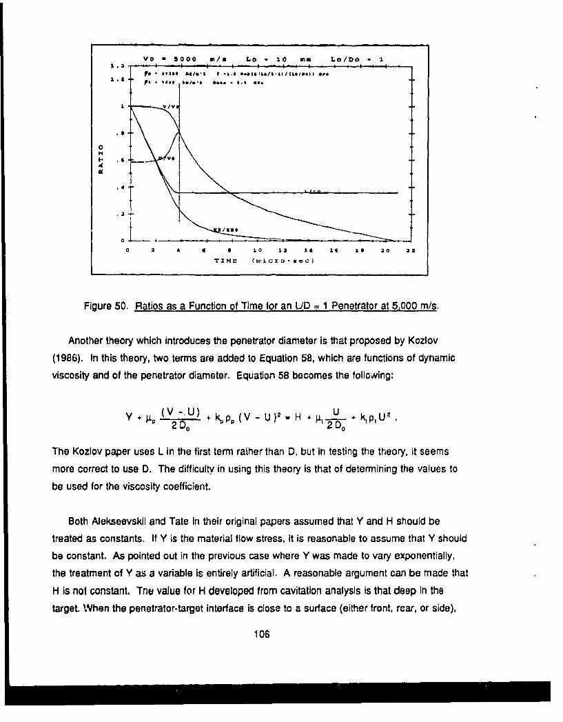
Vo - 5000 M/J L, - 10 MA Lo/Do - 11.2 lIo - -T|I -(lUj | " i-,itJDl f/--"-~tJO~ -t

0 p t - i..rn J... I 1. 120

T I0a

250-2-D

.0

0 -

o* . V. o 1I 14 1 1 0 2

TZMI• (n,jcro;-ui;c)

Figure 50. Ratios as a, Function of Time for an LiD =1 Penetrator at 5.000 rn/s.

Another theory which introduces the penetrator diameter is that proposed by Kozlov

(1986). In this theory, two terms are added to Equation 58, which are functions of dynamic

viscosity and of the penetrator diameter. Equation 58 becomes the following:

y .,(V2-,U)D + l~p=, (V -U) 2 - H + ~i. 1 -o. k~p,U 2

The Kozlov paper uses L in the first term raiher than D, but in testing the theory, it seems

more correct to use D. The difficulty in using this theory is that of determining the values to

be used for the viscosity coefficient.

Both Alekseevskli and Tate in their original papers assumed that Y and H should be

treated as constants. If Y is the material flow stress, it is reasonable to assume that Y should

be constant. As pointed out in the previous case where Y was made to vary exponentially,

the treatment of Y as a variable is entirely artificial. A reasonable argument can be made that

H is not constant. Tne value for H developed from cavitation analysis Is that deep In the

target When the penetrator-target interface is close to a surface (either front, rear, or side),

106

the target resistance should be less than the resistance in a highly confined deep cavity. Just

how H varies Is not clear. At the front surface, a good estimate of the target resistance can

be made using the Brinell hardness number of the surface (to convert the BHN to pressure in

pascals, multiply by 9.8 x 10e or by 9.8 x 107 for dynes per cm2). Figure 51 shows how H

might vary as a function of depth into the target. The function plotted here is as follows:

H HBN + (H.., - H.HN) (- EXP [-oP] ),

with H,. = 5.5 GPa, and the BHN is ,.+u so that H1H = 2.352 GPa. Curves are shown for

c = 50, 100, and 200. P is the depth into the target in meters.

9.3.4 Computer Codes for Numerical Simulation of Impact. The availability of high-speed.

large memory computers has made possible numerical simulation of impact events in either

two dimensions or in three dimensions. Three-dimensional codes are needed to model

oblique impact cases or yawed penetrator cases. The requirements in terms of memory and

execution time for two-dimensional codes are less severe than three-dimensional and are

therefore less costly.

Two approaches have been taken with respect to setting up and running a problem. A

Eulerian grid system remains spatial fixed, and material is transported through the grid. The

Eulerian code is good for problems which involve compressive distortion of material. The

other approach is the Lagrangian grid system in which the mass in each grid cell is constant

and the grid distorts with time. The Lagrangian code is better suited for problems involving

expansive distortion. Some Eulenan codes use a Lagrangian feature of massless tracer

particles to define material package boundaries. In any case, the basic differential equations

which are solved are those of conservaticn of mass, conservation of momentum, and

conservation of energy. Two methods of solution of the equations have been developed-

finite difference and finite element.

The equations which are solved are relatively simple and straightforward. However, they

must be solved in discrete time steps. One of the problems in running a hydrocode is in

selecting a suitable time step. In Eulerian codes, there is a problem of how to handle cells

which contain more than one material (e.g., how to compute densities for the two materials so

107

I

N 34 Ubhn o(hma- -bk5)(G "max'[.cP 0)2

S~(P t.n muter')

S1 311 340

11b)n" 3.352 OP. I~nX S .S l

uI-

10 20 30 40 50 60

Vepth (milli-meotor) (1000 P3

Figure 51. Target Resistance H as a Function of Depth Into the TarQet.

that the material volumes add up to the cell volume if that cell is completely filled or what

should be done it there is void [or gaseous] space In the cell). In Lagrangian codes, the

greatest problem is in when and how to rezone when the cells become greatly distorted, For

both types of codes, it is usually necessary to include one or more slide lines (material

interfaces) where one material is allowed to slide past the other. A number of equations of

state have been developed to compute pressures developed by material under compression

or tension. Failure criteria and how to implement it adds more complexity to solving problems

using hydrocodes.

Some of the hydrocodes which have been used to solve terminal ballistics problems are

as follows:

CSQ - Sandia National Laboratories, Albuquerque, NM.

CTH - Sandia National Laboratories, Albuquerque, NM.

DYNA2,D - Lawrence Uvermore National Laboratory, Livermore, CA.

DYNA3D

108

EPIC-2 - Honeywell, Inc., Brooklyn Park, MN.

EPIC-3

HELP - Systems, Science and Software, La Jolla, CA.

HEMP - Lawrence Uvermore National Laboratory, Livermore, CA.

HEMP3D

HULL - Orlando Technology, Inc., Shalimar, FL

MESA - Los Alamos National Laboratory, Los Alamos, NM.

TOODY - Sandia National Laboratories, Albuquerque, NM.

Some of the equations of state which have been used are as follows.

JWL (Jones, Wilkins, and Lee)

Los Alamos

Mie-Gruneisen

Tillotson

Wilkins

For more information about the previous codes, refer to Zukas (1991).

109


110

10. REFERENCES

Alekseevskil, V. P. "Penetration of a Rod Into a Target at High Velocity." Fizilka-Goreniva/Vzryva vol. 2, no. 2, pp. 99-186 (Combustion, Explosion and Shock Waves, pp. 63-66),1966.

Arbuckle, A. L., E. L Herr, and A. J. Ricohlazzi, "A Computerized Method of ObtainingBehind-the-Target Data From Orthogonal Flash Radiographs," BRL-MR-2264, U.S. ArmyBallistic Research Laboratory, Aberdeen Proving Ground, MD, January 1973.(AD 908362L.)

Backman, M. E., and W. Goldsmith. "The Mechanics of Penetration of Projectiles IntoTargets." International-Journal of Engineering Science, vol. 16, no. 1-A, U.S. NavalWeapons Center, China Lake, CA, 1978.

Baker, W. E., P. S. Westine, and F. T, Dodge. Similarity Methods in Enqineerinq Dynamics.Rochelle Park, NJ: Hayden Book Company, 1973.

Baumeister, T., and L. S. Marks, eds. Standard Handbook F c." Mechanical Engineers.7th ed., McGraw Hill Book Company, pp. 5-16 and 5-17, 1967.

Bjerke, T. W., G. F. SIlsby, D. M. Scheffler, and R. M. Mudd. "Yawed Long Rod ArmorPenetration at Ordnance and Higher Velocities." BRL-TR-3221, U.S. Army BallisticResewarc Laboratory, Aberdeen Proving Ground, MD, March 1991.

Bjerke, T. W., J. Zukas, and K. Kimsey. "Penetration Performance of Tungsten AlloyPenetrators with L/D Ratios of 1 to 1/32." BRL-TR-3246, U.S. Army Ballistic ResearchLaboratory, Aberdeen Proving Ground, MD, June 1991.

Ference, M., Jr., H. B. Lemon, and R. J. Stephenson. Analytical Experimental Physics. 'CheUniversity of Chicago Press, 1956.

Frank, K., and J. Zook. "Energy-Efficient Penetration and Perforation of Targets in theHypervelocity Regire." Proceedings of the 1986 Hypervelocity Impact Symposium.International Journal of Impact Engineering, vol. 5, pp. 277-284, 1987.

Frank, K., and J. A. Zook. "Energy-Efficient Penetration of Targets." BRL-MR-3885, U.S.Army Ballistic Research L.aboratory, Aberdeen Proving Grond, MD, February 1991.

Golub, A., and F. E. Grubbs. "On Estimating Ballistic Limit and Its Precision." BRL-TN-151,U.S. Army Ballistic Research Laboratory, Aberdeen Proving Ground, MD, March 1950.(AD 51120)

Golub, A., and F. E. Grubbs. "Analysis of Sensitivity Experiment's When the Levels ofStimulus Cannot Be Controlled." American Statistical Association Journal, pp, 251-265,June 1956.

111

Goodier, J. N, 'On the Mechanics of Indentation and Cratering in Solid Targets ofStrain-Hardening Metal by Impact of Hard and Soft Spheres." Proceedings-of the=SeventhHvper-Veloclty Impact-Symoslum1 Volume Ill -Theory, pp. 215--259, Orlando, FL, 1965.

Grabarek, C. L. "Penetration of Armor by Steel and High Density Penetrators."BRL-MR-2134, U.S. Army Ballistic Research Laboratory, Aberdeen Proving Ground, MD,October 1971. (AD 518394L)

Grabarek, C. L. 'An Armor Penetration Predictive Scheme for Small Arms AP Ammunition.'BRL-MR-2620, U.S. Army Ballistic Research Laboratory, Aberdeen Proving Ground, MD,April 1976. (AD C006096L)

Grabarek, C. L., and E. L. Herr. 'X-ray Multi-Flash System for Measurement of ProjectilePerformance at the Target." BRL-TN-1 634, U.S. Army Ballistic Research Laboratory,Aberdeen Proving Ground, MD, Septeniber 1966. (AD807619)

Gray, D. E., ed. American Institute of Physics Handbook. 3rd ed.. New York, NY: McGraw-Hill Book Company. pp. 2-39, 1972.

Hagan, J. S., and V. Visnaw. "Analysis of Sensitivity Data following A Normal Distribution.'Analytical Section Report 70-A5-K3, Materiel Test Directorate, October 1970.

Hanagud, S., and B. Ross. "Large Deformation, Deep Penetration Theory for a CompressibleStrain-Hardening Target Material." AIAA Journal, vol. 9, no. 5, 1971, p. 905ff.

Herr, L., and C. L. Grabarek. "Ballistic Performance and Beyond Armor Data For RodsImpacting Steel Armor Plates." BRL-MR-2575, Aberdeen Proving Ground, MD, AberdeenProving Ground, MD, January 1976. (AD B009979L)

Herr, E. L., and C. L. Grabarek. 'Standardizing the Evaluation of Candidate Materials forHigh L/D Penetrators." BRL-MR-2860, U.S. Army Ballistic Research Laboratory, AberdeenProving Ground, MD, September 1978. (AD A062101)

Hill, R. The Mathematical Theory of Plasticity. Oxford: Clarendon Press, 1950.

Hopkins, H. G. "Dynamic Expansion of Spherical Cavities in Metals." Progress in SolidMechanics, vol. 1, chap. 3, edited by I. N. Sneddon and R. Hill, Amsterdam, NY: North-Holland Publishing Company, 1960.

Johnson, W. Impact Strength of Materials. London: Edward Arnold, New York: Crane,Russak, 1972.

Johnson, J. R., and R. E. Mioduski. "Estimation of the Loss of Velocity and Mass ofFragments During Target Perforation." BRL-MR-1 777, U.S. Army Ballistic ResearchLaboratory, Aberdeen Proving Ground, MD, September 1966. (AD 376474)

112

Kozlov, V. S. "Penetration Model That Accounts for the Ductile Properties of the Materialsof Colliding Bodies.* Translated from Problemy Prochnosti, no. 3, pp. 47-52, March 1986.Translation by Plenum Publishing Company, UDC 532.5.032, pp. 334-341, 1986.

Lambert, J. P. "The Terminal Ballistics of Certain 65 Gram Long Rod Penetrators ImpactingSteel Armor Plate.' BRL-TR-2072, U.S. Army Ballistic Research Laboratory, AberdeenProving Ground, MD, May 1978.

Lambert, J. P., and G. H. Jonas. *Towards Standardization In Terminal Ballistics Testing:Velocity Representation.* BRL-R-1852, U.S. Army Ballistic Research Laboratory, AberdeenProving Ground, MD, January 1976. (AD A021389)

MIL-A-1256OG(MR). "Armor Plate, Steel, Wrought, Homogeneous (for Use in Combat-

Vehicles and for Ammunition Testing)." 5 August 1984.

MIL-A-46100C. "Armor Plate, Steel, Wrought, High Hardness." 13 June 1983.

MIL-S-13e12B(MR). "Steel Plate, Wrought, Homogeneous for Ammunition Testing (1/4 TO 12Inches, Inc[.).' 8 February 1171.

Misey, J. "Analysis of Ballistic L!mlt." BRL-MR-2815, U.S. Army Ballistic ResearchLaboratory, Aberdeen Proving Ground, MD, March 1978.

Oberg, E., F. D. Jones, and H. L. Holbrook. Machlnery's Handbook, p. 308, 21st ed.,New York, NY: Industrial Press, Inc., 1979.

Project THOR. "The Resistance of Various Metallic Materials to Perforation by SteelFragments; Empirical Relationships for Fragment Residual Velocity and Residual Weight."TR-47, U.S. Army Ballistc Analysis Laboratory, Institute for CooperativeResearch, The Johns Hopkins University, April 1961.

Project THOR. "The Resistance of Various Non-Metalic Materials to Perforation by SteelFragments; Empirical Relationships for Fragment Residual Velocity and Residual Weight."TR-51, Ballistic Analysis Laboratory, Institute for Cooperative Research, The Johns HopkinsUniversity, April 1963.

U.S. Army Materiel Command. Engineering Design Handbook, Elements of ArmamentEngflneering, Part 2: Ballistics. AMCP 706-107, September 1963.

Roecker, E., and C. L. Grabarek. "The Effect of Yaw and Pitch on Long Rod Penetration IntoRolled Homogeneous Armor at Various Obliquities." Proceedings of the Ninth InternationalSymposium on Ballistics, Royal Military College of Science, Shrivenham, England, 29 Apr-1May 1986.

SIlsby, G. F. "Penetration of Semi-infinite Steel Targets by Tungsteii Long Rods at 1.3 to4.5 km/s." Proceedings of the Eighth International Symposium on Ballistics, Orlando FL,1984.

113

Silsby, G. F., R. J. Roszak, and L. Giglio-Tos. "BRL's 50-mm High Pressure Powder Gun forTerminal Ballistic Testing - The First Year's Experence." BRL-MR-03236, U.S. ArmyBallistic Research Laboratory, Aberdeen Proving Ground, MD, January 1983.

Tate, A. "A Theory for the Deceleration of Long Rods After Impact." Journal of theMechanics and Physics of Solids, vol. 15, pp. 387-399, 1967.

Tate, A. "Further Results in the Theory of Long Rod Penetration." Journal of the Mechanicsand-Physics of Solids, vol. 17, pp, 141-150, 1969.

Tate, A, "Lorg Rod Penetration Models - Part I. A Flow Field Model For High Speed LongRod Penetration." International-Journal of Mechanical Sciences, vol. 28, no. 8,pp. 535-548, 1986a.

Tate, A. "Long Rod Penetration Models - Part I1. Extensions to the Hydrodynamic Theory ofPenotration." International Journal of Mechanical Sciences, vol. 28, no. 9, pp. 599-612,1986b.

Taylor, G. i. "The Use of Flat-Ended Projectiles for Determining Dynamic Yield Stress, I:Theoretical Consideration." Proceedinals of the Royal Society of London, A194, 289, 1948.

Walters, W. P., and J. A. Zukas. Fundamentals of Shaped Charges. John Wiley and Sons,Inc., 1989.

Wilkins, M. L., and M. W. Guinan. "Impact of Cylinders on a Rigid Boundary." Journal ofApplied Physics, vol. 44, no. 3, pp. 1200--1206, March 1973.

Zook, J. "An Analytical Model of Kinetic Energy Projectile/Fragment Penetration."BRL-MR-2797, U.S. Army Ballistic Research Laboratory, Aberdeen Proving Ground, MD,October 1977.

Zook, J. A., and D. F. Merritt. "Advanced Techniques for Analyzing Dynamic Fragments."BRL-MR-3313, U.S. Army Ballistic Research Laboratory, Aberdeen Proving Ground, MD,October 1983. (AD ADA 134348)

Zook, J., W. Slack, and B. lzdebski. "Rizochet and Penetration of Steel Spheres ImpactingAluminum Targets." BRL-MR-3243, U.S. Army Ballistic Research Laboratory, AberdeenProving Ground, MD, February 1983. (AD A125330)

Zukas, J. A., ed. High Velocity Impact Dynamics, John Wiley and Sons, Inc., 1991.

Zukas, J. A., T. Nicholas, H. F. Swift, L. B. Greszczuk, and D. R. Curran. Impact Dynamics.John Wiley and Sons, Inc., 1982.

114

BIBLIOGRAPHY

Backman, M. E. *Terminal Ballistics." NWC TP 5780, Naval Weapons Center, China Lake,CA, February 1976.

Brown, C. J. "Estimates of Residual Mass and Velocity for Tungsten and Steel Fragments."BRL-MR-2794, U.S. Army Ballistic 9esearch Laboratory, Aberdeon Proving Ground, MD,October 1977.

Dehn, J. T. "The Particle Dynamics of Target Penetration." BRL-TR-02188, U.S. ArmyBallistic Research Laboratory, Aberdeen Proving Cround, P ID, Saplember 1979.

Dehn, J. T. "A Unified Theory of Penetration." BRL-TR-2770, U.S. Army Ballistic ResearchLaboratory, Aberdeen Proving Ground, MD, December 1986.

Farrand, T. G. "A Database Storage System and the Sonic Digitizer Method for RadiographicData Reduction Used by the Penetration Mechanics Branch." BRL-MR-3847, U.S. ArmyBallistic Research Laboratory, Aberdeen Proving Ground, MD, June 1990.

Hauver, G. E., and A. Melani. "Behavior of Segmented Rods During Penetration,"BRL-TR-3129, U.S. Army Ballistic Research Laboratory, Aberdeen Proving Ground, MD,July 1990.

Kimsey, K. D., and J. A. Zukas. "Contact Surface Erosion for Hypervelocity Problems."BRL-MR-3495, U.S. Army Ballistic Research Laboratory, Aberden Proving Ground, MD,February 1986.

Kineke, J. H., Jr., and C. E. West, Jr. "Perforation Area Produced by Fragment Impact."BRL-TR-02580, U.S. Army Ballistic Research Laboratory, Aberdeen Proving Ground, MD,August 1984.

Lambert, J. P., and B. E. Ringers. "Standardization of Terminal Ba'listics Testing, DataStorage and Retrieval." BRL-TR-02066, U.S. Army Ballistic Research Laboratory, AberdeenProving Ground, MD, May 1978.

Merritt, D. F., and C. E. Anderson, Jr. "X-ray Trigger Predictor: Automatic Electronic TimeDelay Device for Flash X-ray Systems." BRL-TR-02284, U.S. Army Ballistic ResearchLaboratory, Aberdeen Proving Ground, MD, January 1981.

Rapacki, E. J. "Instrumentation Techniques for Measuring Large, High Rate Strains With FoilResistance Strain Gages." BRL-TR-02573, U.S. Army Ballistic Research Laboratory,Aberdeen Proving Ground, MD, August 1984.

Scheffler, D. R., and T. M. Sherrick. "Large-Scale Simulations of Monolithic and SegmentedProjectiles Impacting Spaced Armor." BRL-TR-3080, U.S. Army Ballistic ResearchLaboratory, Aberdeen Proving Ground, MD, February 1990.

115

SlIsby, G. F. "Rectification of Multiflash Radiographs." BRL-MR-03363, U.S. ArmyBallistic Research Laboratory, Aberdeen Proving Ground, MD, July 1984.

Walters, W. P., and S. B. Segletes. "Solution of the Long Rod Penetration Equations."BRL-TR-3180, U.S. Army Ballistic Research Laboratory, Aberdeen Proving Ground, MD,December 1990.

Wilbeck, J. S., C. E. Anderson, Jr., J. P. Riegel, Ill, J. Lankford, S. A. Mullin, and S. R.Bodner. "A Short Course on Penetration Mechanics." Course Notes, Southwest ResearchInstitute, San Antonio, TX.

Wright, T. W., and K. Frank. "Approaches to Penetration Problems." BRL-TR-2957, U.S.Army Ballistic Research Laboratory, Aberdeen Proving Ground, MD, December 1988.

Zook, J. A., and K. Frank. "Comparative Penetration Performance of Tungsten Alloy L/D = 10Long Rods With Different Nose Shapes Fired at Rolled Homogeneous Armor."BRL-MR-3480, U.S. Army Ballistic Research Laboratory, Aberdeen Proving Ground, MD,November 1985.

Zook, J. A., C. J, Brown, and C. L. Grabarek. "The Penetration Performance of TungstenAlloy L/D = 10 Long Rods With Different Nose Shapes Fired at Rolled HomogeneousAmr r." BRL-MR-03350, U.S. Army Ballistic Research Laboratory, Aberdeen ProvingGround, MD, April 1984.

Zukas, J A. "Impact Dynamics: Theory and Experiment." BRL-TR-02271, U.S. Army BallisticResearch Laboratory, Aberdeen Proving Ground, MD, October 1980.

Zukas, J. A. "Numerical Simulation of Semi-infinite Target Penetration by Continuous andSegmented Rods." BRL-TR-3081, U.S. Army Ballistic Research Laboratory, AberdeenProving Ground, MD, February 1990.

116

GLOSSARY

ballistic limit - The striking velocity required to just perforate the target configuration (residualvelocity of 0). (Army, Navy, and protection criteria define different methods ofdetermining whether a result Is a perforation or a penetration.) Can also refer to the angleof obliquity at a particular striking velocity which will result in zero residual velocity (the 06.

bore - The hollow cylindrical shaped center portion of a gun barrel,

Brinell hardness number (BHN) - A measure of hardness of the surface of the test specimenbased on the diameter of indentation of a sphere (usually 10 mm In diameter) under staticpressure (hydraulic press), usually 3,000 kg/mm2.

caliber - The diameter of the bore of the barrel of a gun.

carrier - The sabot assembly-consists of the obturator, pusher plate, and sabot (the latterenvelops the penetrator).

center of mass - The point In a rigid body which moves as if all of the mass of the body andall of the forces acting on the body were concentrated at that point.

Charpy impact test - A measure of a test specimen's resistance to fracture.

ductile - Capable of being drawn out or hammered thin,

empirical - Based on experimental data only without regard to theory or scientific principles.

erosion - The disintegration of the penetrator at the penetrator-target interface due to forcesacting at the interface.

exit angle - The angle which the path of the residual penetrator makes with the original shotline after perforating a target.

fiducial - A reference marker.

high hardness armor (HHA) - Steel armor made to meet Army specifications as described inMIL-A-46100C (1983).

K factor - The magnification factor,

magnification factor - The ratio of the size of the object which creates an image onphotographic film (due to radiation from a point source) to the size of the imageappearing on the film.

maximum likelihood - A procedure to determine the most likely value of the average of valueswhich constitute a zone of mixed results (perforations occurring at velocities below that ofnonperforating velocities for a particular penetrator/target configuration).

117

munition - An abbreviation of ammunition.

normal - Perpendicular (900 angle) to the surface.

obliquity - The angle which the shot line makes with a line perpendicular (normal) to thesurface oi the target at the point of intersection of both lines.

obturator - The rear portion of the sabot assembly which provides a gas seal to prevent thegasses produced by the burning propellant from escaping In the forward direction while theprojectile is travelling down the gun barrel.

orthogonal - At a 900 angle.

partial penetration - A penetrator/target interaction in which the penetrator does not exit thetarget (a penetration as opposed to a perforation).

penetration - A penetrator/target interaction in which the penetrator does not exit the target.

penetrator - The part of a projectile which Impacts the target and is responsible for penetratingor perforating the target.

perforation - A penetrator/target interaction In which the penetrator defeats the target (light canbe seen through the hole made by the penetrator).

pitch - The angle that a projectile makes with the flight path when measured in the verticalplane -projectile is tilted either up or down with respect to the flight path.

projectile - A body which is undergoing free flight.

propellant - The chemical explosive which, when initiated, causes the projectile to acceleratedown the gun barrel.

pusher plate - Metal disc which is part of the sabot assembly and absorbs the setback forcesupon launching the projectile.

radiography - Photography which uses invisible high-frequency radiation such as x-rays orgamma rays to expose the film.

residual velocity - The speed (velocity if the exit angle is included) of the residual penetratorafter perforating a target plate.

residual mass - The mass of the portion of the penetrator which exits the target afterperforating the target.

Rockwell hardness (Re) - A measure of the hardness of the surface of a test specimen using aconic-shaped irndentor rather than the spherical indentor of the Brinell hardness test. Thesubscript c refers to the size of the Indentor.

118

rolled homogeneous armor (RHA) - Steel armor plate made to meet Army militaryspecifications as described In MIL-A-12560F(MR) (1984).

sabot - The part of the sabot assembly which envelops the subcaliber penetrator making upthe difference between the diameter of the penetrator and the diameter of the bore of thegun barrel.

semi-infinite - A term used to describe a target which is sufficiently thick so that the rearsurface does not influence the result of the Impact (requires the penetrator to come to restwithin the target).

stabilization - The condition in which a projectile in free flight reaches an equilibrium state withrespect to forý,us which cause it to precess (wobble) about its main axis.

striking velocity - The speed (velocity when the obliquity is Included) at which the penetratorimpacts the target plate.

subcaliber - A diameter which is less than the diameter of the bore of the associated gun

barrel.

target - Material which the projectile is intended to Impact.

theta 50 - The angle of obliquity which defines the boundary between penetration andperforation for a penetrator Impacting at a specific impact velocity (symbollically, e).

V50 - The ballisfic limit determined by taking the average of an equal number of perforationsand penetrations (usually three of each, which makes a six-round V.,.) within a specifiedImpact velocity range (125 ft/s).

Vicker's test - A measure of the strength of a material.

witness pack - A series of metal plates of varying thickness separated by styrofoam sheetswhich is used to record the debris (including the residual penetrator) which emanates froma target which has been perforated. 4k

witness panel - A single sheet of material placed behind the target which exhibits thedistribution pattern of impacting debris emanating from a target upon being perforated.

yaw - The angle that the axis of a projectile makes with the flight path when measured in thehorizontal plane - projectile is tilted sideways with respect to the flight path. Note:Sometimes yaw refers to the maximum deviation angle of the axis of the projectile withrespect to the flight path measured in the plane of maximum deviation.

119

INTFENTIONALLY LEFT BLANK.

120

No. of No. ofQ .Organizatlon Coles Omanizon

2 Administrator I CommanderDefense Technical Info Center U.S. Army Missile CommandATrN: DTIC-DDA ATTN: AMSMI-RD-CS-R (DOC)Cameron Station Redstone Arsenal, AL 35898-5010Alexandria, VA 22304-6145

1 CommanderCommander U.S. Army Tank-Automotive CommandU.S. Army Materiel Command ATTN: ASQNC-TAC.DIT (TechnicalATiN: AMCAM Information Center)5001 Eisenhower Avenue Warren, MI 48397-S000Alexandria, VA .2333-0001

1 DirectorCommander U.S. Army TRADOC Analysis CommandU.S. Army Laboratory Command ATTN: ATRC-WSRATTN: AMSLC-DL White Sands Missile Range, NM 88002-55022800 Powder Mill RoadAdelphi, MD 20783-1145 1 Commandant

U.S. Army Field Artillery School2 Commander ATTN: ATSF-CSI

U.S. Army Armament Research, Ft. Sill, OK 73503-5000Development, and Engineering Center

ATTN: SMCAR-IMI-l (Mon.. aI1y)I CommandantPicatinny Arsenal, NJ 07806-5000 U.S. Army Infantry School

ATTN: ATSH-CD (Security Mgr.)2 Commander Fort Benning, GA 31905-5660

U.S. Army Armament Research,Development, and Engineering Center (Un*,a,. an)1 Commandant

ATTN: SMCAR-TDC U.S. Army Infantry SchoolPicatinny Arsenal, NJ 07806-5000 ATTN: ATSH-CD-CSO-OR

Fort Benning, GA 31905-5660DirectorBenet Weapons Laboratory 1 Air Force Armament LaboratoryU.S. Army Armament Research, ATTN: WLJMNOI

Development, and Engineering Center Eglin AFB, FL 32542-5000ATTN: SMCAR-CCB-TLWatervliet, NY 12189-4050 Aberdeen Provina Ground

(Unca.. onty)l Commander 2 Dir, USAMSAAU.S. Army Armament, Munitions ATTN: AMXSY-D

and Chemical Command AMXSY-MP, H. CohenATTN: AMSMC-IMF-LRock Island, IL 61299-5000 1 Cdr, USATECOM

ATTN: AMSTE-TCDirectorU.S. Army Aviation Research 3 Cdr, CRDEC, AMCCOM

and Technology Activity ATTN: SMCCR-RSP-AATTN: SAVRT-R (Library) SMCCR-MUM/S 219-3 SMCCR-MSIAmes Research CenterMoffett Field, CA 94035-1000 1 Dir, VLAMO

ATTN: AMSLC-VL-D

10 DIr, BRLATTN: SLCBR-DD-T

121

No. ofCooler Omaniztilon

I SouthWest Research Institute6220 Culebra RoadATTN: Dr. Charles Anderson, Jr.Postal Drawer 28510San Antonio, TX 78284

122

USER EVALUATION SHEET/CHANGE OF ADDRESS

This laboratory undertakes a continuing effort to improve the quality of the reports itpublishes. Your comments/answers below will aid us in our efforts.

1. Does this report satisfy a need? (Comment on purpose, related project, or other area ofInterest for which the report will be used.)

2. How, specifically, Is the report being used? (Information source, design data, procedure,source of ideas, etc.)

3. Has the information in this report led to any quantitative savings as far as man-hours ordollars saved, operating costs avoided, or efficiencies achieved, etc? If so, pleaseelaborate.

4. General Commpnts. What do you think should be changed to improve future reports?(Indicate changes to organization, technical content, format, etc.)

BRL Report Number BRL-MR-3960 Division Symbol

Check here if desire to be removed from distribution list.

Check here for address change.

Current address: OrganizationAddress

DEPARTMENT OF THE ARMYDirector NO POSTAGEU.S. Army Ballistic Research Laboratory NECE SSARGYATTN: SLCBR-DD-T AIEDAberdeen Proving Ground, MD 21005.5066 I FM ILEOIN THE

OFCIAL BUSINESS BUSINESS REPLY MABU USIE

E! RRST WO PERMIT No 0001, APS, MO

PoLlage will be paid by addressee

Director -U.S. Army Ballistic Research Laboratory _ ____

ATTN: SLCBR-DD-TAberdeen Proving Ground, MD 21005-5066 I ]

dtc john a. zook ~ ~;~konr~ad 1992 january 1992ad--a246 922 memorandum report brl-mr-3960 terminal...

Documents