8

Mark Bryan Emilia Del Bono Stephen Pudney

Institute for Social and Economic Research

University of Essex

No. 2013-08 July 2013

ISE

R W

ork

ing P

aper S

erie

s

ww

w.is

er.e

sse

x.a

c.u

k

Drug-related crime

Non-technical summary Drug-related crime is estimated to account for a large part of the economic and social costs of

illicit drug use and also to make up a large share of total crime. However, when measuring

criminal activity it is extremely difficult to disentangle crime which is directly caused by drug

use from crime that is linked to drug use but is caused by other factors. The distinction is

important because, when evaluating the costs or benefits of drug policy reform, only crime

which is caused by drug use should be considered. This study discusses this concept of drug-

related crime, reviews methods for estimating it and produces estimates of drug-related crime

in England and Wales in 2003-6.

We provide a critical discussion of the concept of drug-related crime, arguing that the relevant

comparison is not between existing crime levels and those in a world without drugs, but

between existing crime levels and those that would exist under plausible reforms to drug policy.

We consider three illustrative policy scenarios: (i) a benchmark, but unrealistic, scenario in

which drugs are unavailable; (ii) free supply of drugs to dependent users (e.g. supervised

injection) that would avoid recourse to the illegal market; and (iii) the introduction of a

regulated drug supply that changes market prices. We discuss how accurately standard

comparison methods (using data on drug users and the criminal behaviour) measure drug-

related crime under each scenario.

We then derive estimates of drug-related crime using four alternative comparison methods

applied to survey data from England and Wales. To ensure full coverage of the population while

including sufficient numbers of drug users and individuals who have committed crime, we

combine the household-based Offending Crime and Justice Survey and the Arrestee Survey

conducted in police arrest facilities. We focus on three groups: heroin users, cannabis users (not

involved with heroin or cocaine) and cannabis suppliers.

We find three key results. First, the volume of drug-induced acquisitive crime linked to heroin

use is high, at 160-230 offences a year for heroin users generally and 200-260 offences for

heroin injectors. However, there is no significant evidence of violent crime linked directly to

heroin use (although heroin suppliers may be involved in violent crime). Second, we find no

evidence at all of any drug-induced crime committed by people who only use cannabis. Third,

we find evidence that supplying cannabis (only) leads to a small volume of crime, amounting to

2.5-9 acquisitive offences and 0.9-2.7 violent offences on average per year. The mechanisms

linking cannabis supply to criminal activity merit further investigation.

Drug-related crime

Mark Bryan

Emilia Del Bono

Stephen Pudney

Institute for Social and Economic Research University of Essex

This version 1 July 2013

Abstract: We provide a critical discussion of the concept drug-related crime and review methods for estimating its volume, emphasising the importance of an appropriately defined counterfactual. We then construct new estimates for England and Wales in 2003-6, combining data from the Arrestee Survey and Offending Crime and Justice Survey to ensure adequate coverage of prolific offenders/drug users and non-household residents, who are under-represented in household surveys. We find, first, that the volume of drug-induced acquisitive crime linked to heroin use is high, but there is no significant evidence of violent crime linked directly to heroin use. Second, we find no evidence at all of any drug-induced crime committed by people who use cannabis (but not heroin or cocaine). Third, we find evidence that supplying cannabis leads to a small volume of crime. The mechanisms linking cannabis supply to criminal activity merit further investigation. Keywords: Illicit drugs, Crime, Matching estimators JEL codes: C21, K42 Contact: Steve Pudney, ISER, University of Essex, Wivenhoe Park, Colchester, CO4 3SQ, UK. Email: spudney@essex.ac.uk; Tel: +44-(0)1206 873789 This work was supported by funding from the Open Society Institutes. The views expressed here are our own and not necessarily those of the OSI. We are grateful to Marta Favara for valuable research assistance and to Richard Layard for helpful comments.

1

1 Introduction

Drug-related crime undoubtedly accounts for a large part of the external costs of illicit drug use.

For example, Godfrey et al (2002) estimated that around 88% of the economic and social costs of

class A drug use in England and Wales in 2000 was attributable to crime and policing costs,

while the UK Drug Harm Index (MacDonald et al. 2005, 2006), which attempts to measure the

trend over time in drug-related social harms, assigns over two-thirds of its weight to property

crime. For Australia in 2004/5, Collins and Lapsley (2008) estimate that 41-51% of crime was

attributable to drug use and that crime was responsible for 56% of the tangible costs arising

from illicit drugs in 2004/5. The ONDCP (2004) gives broadly similar estimates for the US.

A better term for the concept at issue here is drug-induced crime, since we are concerned with

crime that is causally related to drug use. In a much-cited paper, Goldstein (1985) made a

distinction between three types of drug-induced crime.1 “Economic-compulsive” crime arises

from a need for additional income to fund the drug purchases made necessary by compulsive

drug use. “Psychopharmacological” crime is behaviour generated by the action of drugs on the

brain, resulting in weakened self-control or decision-making capacity, or violent responses to

external provocation. “Systemic” violence is seen as a feature of the working of illicit markets,

where legal enforcement of contracts is impossible. Note that economic-compulsive crime may

relate to any form of strongly-desired consumption, not only illicit drugs – some people may

commit crime to generate money to buy alcohol, tobacco, clothes, etc. To these direct forms of

drug-related crime, we could add long-run indirect effects which are hard to evaluate but may be

important. For instance, if drug use impairs intellectual ability, educational achievement and

employment prospects, acquisitive crime becomes more rewarding relative to legal income-

generating activity and crime becomes a ‘rational’ response to lack of opportunity for some.

There is a large research literature on drug-related crime and some empirical associations are

consistently observed (see Stevens et al 2005 for a survey), but the direction of causation is

unclear, and crime is often found to precede drug use in individual offending careers

(Hammersley et al 1989, Pudney 2003, D’Amico et al 2008, Hales et al 2009). Heroin use is

associated with high rates of acquisitive but not violent crime (Hammersley et al 1989, Fischer

et al 2001) but there is a weaker association between cannabis use and acquisitive crime, and

research on the effects of cannabis on the brain does not suggest a link to violence (Hoaken and

Stewart 2003). Systemic crime linked to the cannabis market may be particularly important in

some particular instances, such as the recent gang violence in Mexico largely attributable to

supply to the US marijuana market, and some episodes of human trafficking and exploitation

linked to cannabis production in the UK. The few studies of other markets subject to exogenous

1 See Bennett and Holloway (2009) for a critique.

2

switches in legality suggest significant increases in systemic violent crime as a consequence of

the banning of a previously legal market (see Miron 1999 on alcohol prohibition and Chimeli and

Soares 2011 on the Brazilian mahogany trade).

Research is hampered by the difficulty of estimating the counterfactual level of crime that would

have been committed by drug users or suppliers in the absence of drugs. The usual difficulty of

establishing causality in a non-experimental setting is particularly important here because, as

pointed out by Burr (1987), drug consumption and criminal activity are choices made by the

individual. What does it mean to say that drug use causes crime, if they are joint outcomes of the

same choice? This question, addressed in sections 2.1-2.4 below, is often neglected in the applied

literature and in the statistical literature on causal inference.

2 Concepts and methods

In 1998, the United Nations General Assembly Special Session (UNGASS) adopted the slogan “A

drug free world - we can do it!”, and the conceptually loose definition of drug-related crime which

implicitly underpins most attempts at measurement reflects this:

Definition: The volume of drug-related crime is the difference between the volume of crime in

the world as it is and the volume of crime that would exist in an otherwise identical world with

illicit drugs unavailable.

This is not a helpful definition, for at least two reasons. First, despite the UNGASS display of

confidence, a drug-free world is completely implausible and other policy-related counterfactuals

are of more practical interest. In practice, we are interested in some change in the policy regime

which may alter (but not reduce to zero) the level of drug use. A second problem with the

definition is that the nature of the counterfactual is likely to depend on the means by which it is

achieved. A world with drugs eliminated by a perfectly successful programme of interdiction and

incarceration of drug traffickers would look very different from a world with drugs eliminated

by a successful public information and education campaign.

Liberalisation of cannabis supply and the provision of clinics for supervised injection of

prescribed heroin are two examples of counterfactuals that arise in current policy debates. They

are useful examples, because they involve drug-induced crime in conceptually different ways, as

discussed in sections 2.3-2.4. However, no modern country has yet pursued supply liberalisation

to the full extent of legalisation and there have only been small local experiments with

supervised heroin injection, which we review in section 8 below.

We first consider the conceptual basis for measurement under the UNGASS counterfactual, and

then examine the issues involved in moving to more realistic policy-related counterfactuals.

Given the uncertainties involved in measurement, it is unreasonable to expect a single fully

3

defensible estimate of the volume of drug-induced crime. Instead, our strategy is to use a

number of different survey-based approaches to indicate the range of plausible estimates, and

then compare these estimates with the effects identified by the few experimental studies that

exist. Our data are summarised in section 3 and implementation of the methods in section 4.

Results are presented in sections 5-7 and compared to existing experimental evidence in section

8. The implications of our findings for the social cost of drug use are considered in section 9.

2.1 Concepts of drug-induced crime

There are conceptual difficulties arising from the fact that drug use is a choice rather than a

‘treatment’. We use an illustrative single-period choice theory of drug demand which, although

too simple to be a full description of demand behaviour, captures the nature of the measurement

problem. It also emphasises an important point often overlooked in the medical literature: that

drug users – however ‘addicted’ they may be – are consumers and respond to economic

incentives in much the same way as the consumers of other goods.

Assume a single illicit drug h with market price p. Criminal activity yields disutility rather than

consumption benefits but can be used as income-generating activity. Individuals behave in

accordance with the following utility maximisation programme:

(1)

subject to: (2)

where q is expenditure on legal consumption goods, c is criminal activity, U(.) is increasing in h

and q and decreasing in c, is the rate of return to crime and b is legal income. The programme

(1)-(2) has solutions for drug use and crime and which divide individuals

into two groups: drug users, for whom , and non-users, for whom .

Now impose the counterfactual intervention as a further restriction h = 0, assuming no general-

equilibrium effects causing b and to change. The new outcome is , where

if , since non-users are unaffected by withdrawal of drug supply. The impact on

the criminal behaviour of those who are drug users under the status quo is , which is the

“average effect of treatment on the treated” (ATT) in the language of causal inference. That

terminology is inexact here, because drug use is choice rather than treatment and the “non-

treated” are only unaffected because of the nature of their choices. For that reason, we refer to

the impact as a pseudo-ATT (PATT), defined as:

(3)

The aggregate per capita volume of drug-induced crime is then the product of the PATT and the

drug prevalence rate. None of the usual methods for estimating the volume of drug-related crime

4

provides a direct estimate of the PATT. We consider four approaches:

(i) Naive assumption. If drug users would, in the absence of drugs, be crime-free, then :

(4)

This is an implausible assumption, yielding an upper bound on the volume of drug-induced

crime, given the empirical fact that drug use is very often preceded in the development process

by other forms of illegal behaviour (Hales et al 2009, Pudney 2003). Nevertheless, it underpins

much discussion of drugs policy: for example, it is assumed by Godfrey et al (2002) and is

implicit in the construction of the UK Drug Harm Index (MacDonald et al 2005, 2006).

(ii) Exogenous selection into drug use. We could assume more reasonably that, without drugs,

people who are currently users would, on average, have committed the same level of crime as

non-drug users, so that :

(5)

(iv) Matching. The measure (5) ignores the fact that drug users tend to have different

characteristics and personal histories than non-users, and it can be improved by using a

reference group of better-matched non-users to construct the counterfactual. This can be done

using propensity score matching (Rosenbaum and Rubin 1983) or Mahalanobis matching (Rubin

1980, Abadie and Imbens 2006). It requires further information on a set of characteristics

describing the individual and his or her personal history, such that the post-intervention

criminal activity of a drug user with characteristics is, on average, the same as that of a non-

user with the same characteristics, so that :

(6)

(iii) Self-assessed motivation. A fourth approach, pursued for the US by ONDCP (2004) and for

Australia by Collins and Lapsley (2008), is to use drug users’ own assessments, m, of the amount

of their own criminal activity which is induced by their drug use. This embodies the assumption

that and, consequently:

(7)

This too is open to objection on grounds that criminals themselves may be no better at analysing

causation than are social researchers and may find it convenient to blame an external factor for

their own behaviour, leading to overestimation of the volume of drug-induced crime.

2.2 Theoretical validity of comparison methods

The literature on causal inference is dominated by the concept of ‘treatment’, although methods

are often applied in contexts where choice, rather than treatment is involved, with little

5

discussion of the relationship between choice theory and matching methods. None of the four

measures (4)-(7) follows directly from choice theory and, in particular, it is not at all obvious

that the measures PATT2 and PATT3 , based on comparisons between groups of users and non-

users, are consistent with the principles of choice theory. After all, if users and non-users were

entirely comparable, there would be no distinction between the two – either everyone would be

a user or everyone a non-user. So we must allow for the possibility of factors that induce some to

use drugs, while others do not. A separability assumption gives these comparison methods

some theoretical validity. Assume the utility function is:

(8)

where the component functions and are common to all individuals and is

the complete set of personal characteristics, history and circumstances which determine the

form of preferences with respect to crime, drug use and general consumption. Note that is

critical here, since it is responsible for the distinction between drug users and non-users within

the set of people with any particular set of characteristics .

Suppose – implausibly – that a successful interdiction policy causes the constraint to be

imposed directly. Crime is then determined by maximisation of the sub-utility function

subject to the budget constraint and is therefore unaffected by the subset of

characteristics z which only influence crime-consumption choices when the optimal choice

involves drug use. In this model, a drug user with characteristics will, under the drug-free

counterfactual, have crime level identical to that of a non-user who shares the relevant subset of

characteristics, , so that and, provided that is used to perform

the matching, the measure PATT3 is valid. Without the separability assumption (8), matching on

alone is invalid, since acts as an unobserved confounder. On the other hand, if we were to

attempt matching on both and , all individuals would have the same drug use status, so one of

the ‘treatment’ and ‘control’ groups would be empty, and matching would be impossible. The

exclusion of from the consumption-crime subutility means that there exist personal factors

which could predispose the individual to drug use but would not also predispose him/her to a

high crime-high consumption lifestyle. It is possible that genetic variations in brain function

recently identified by neuroscience may fit this role (Mayer and Höllt 2005). The separability

assumption (8) is not unduly restrictive: it allows for Goldstein’s (1985) economic-compulsive

pathway via the budget constraint and also the psychopharmacological pathway since variation

in h may change the marginal rate of substitution between consumption and crime.

Extension of the analysis to more realistic counterfactuals than the hypothetical disappearance

of illicit drug supply may require further assumptions for the validity of user-nonuser

comparisons. We consider two types examples of intervention: supervised heroin injection for

6

addicts; and licensing and regulation of the drug market.

2.3 Other counterfactuals: supervised injection facilities

Consider a policy that makes available to dependent drug users a free supply , used under

supervision. With this intervention in place, there is still access to an illegal drugs market,

allowing participants to raise consumption above the maintenance level by a positive amount

if desired. Supervision means that prescribed drugs cannot be sold to generate

income and, assuming the satiation level is above , utility maximisation is equivalent to:

(10)

At a corner solution with no resort to the black market, (10) reduces to maximisation of

, rather than which is maximised by non-users. Consequently,

and PATT3 is not a reliable guide to the impact of the intervention.

To avoid this problem, we need to make a stronger separability assumption under which

preferences are representable by the utility function

(11)

This implies that the marginal rate of substitution between general consumption and criminal

activity is independent of drug use, ruling out Goldstein’s (1985) psychopharmacological causal

mechanism. Under (11), criminal activity chosen by a drug-using criminal is a function only of

the returns to crime and residual income remaining after paying for drugs. This structure

embodies a definite restriction on the pattern of behaviour but, in the absence of compelling

evidence for the pharmacological mechanism, it is credible as a basis for measurement.

In this case, drug-users operating at a corner solution and non-users both maximise the same

function , so PATT3 is valid. However, the matched control group of

non-users only works perfectly if the drug maintenance level is high enough to prevent all

resort to the illicit market. A drug user operating at an interior solution above the prescribed

dose maximises , which differs from the objective of a non-user.

Consequently, even under this stronger form of separability, we would expect the matching

technique to underestimate the volume of crime in the counterfactual environment, since

purchase of black market drugs is likely to be accompanied by additional criminal activity, and

thus over-estimate the potential crime reduction that induced by the intervention.

2.4 Other counterfactuals: liberalisation of supply

Now consider the case of liberalisation of drug supply and assume that the principal effect of the

policy change is to reduce the market price p. To derive a direct relationship between the effect

7

of this intervention and the PATT, we need to use the full separability assumption (11), implying

that the crime function for a drug-user with characteristics is:

(12)

where is residual income after drug costs. If policy produces a marginal

change, , in the drug price, the impact on crime committed by this drug user is:

(13)

where is the price elasticity of demand for drugs. The pseudo-Engel coefficient is

expected to be negative since high income reduces the incentive for crime. Note first that, if the

drug has a price elasticity of -1, the impact on crime is zero, despite the rise in volume of drug

consumption. It is the drug expenditure response to the price change that matters for acquisitive

crime, not the quantity response. Only if drug demand is inelastic will the impact

on crime be positive. There are few convincing estimates of the price elasticity of heroin but, for

cannabis, several studies suggest a price elasticity around -0.5 (Clements and Zhao 2005, Van

Ours and Williams 2005). If this is true for drug h, the percentage change in crime caused by a

1% price rise will be , which is expected to be positive.

Consequently, rising drug prices increase, rather than reduce, the volume of crime. While drug

‘droughts’ caused by interdiction actions may succeed in reducing consumption and internal

harm to the health of users (Day et al 2003), by raising prices they may also have the perverse

effect of increasing external social harm from drug use. This raises the issue of distributional

equity between drug users and the non-user community.

The PATT measures the impact on crime of a removal of drug supply. To convert this into a

measure of the impact of a price change, multiply by the impact on drug use of a price change .

The appropriate way to do this is in proportionate expenditure terms, giving:

. This gives the correct measure (13) if

, which holds as a tangent approximation since, by the mean value theorem:

(14)

for some point in the interval . This approximation is good if crime choices are

approximately linear in residual income or if drug expenditure is small. If crime is a decreasing

convex function of residual income, use of the PATT will tend to overstate the true impact on

crime. Note that, if PATT is zero, then the impact of a policy-induced price change on drug-

related crime is unambiguously zero.

3 UK survey data

Conventional household-based surveys are poor vehicles for measurement of illegal activity.

8

Prolific offenders and drug users have low survey response rates and some lead disordered lives

which exclude them from standard sampling frames. To improve coverage of groups with high

rates of drug use and criminal activity, we need a complementary survey with better focus on

this group. Since we need to compare the criminal activity of drug-users and non-drug-users,

data from the monitoring records of drug treatment programmes, such as NTORS and DTORS

(Jones et al 2007, 2009), are not suitable, since their samples are conditioned on the existence of

some form of drug dependence. Surveys which select individuals on a crime-related basis (for

example through arrest or imprisonment) are potentially more useful, since they include both

drug users and non-users. All surveys targeted at groups with high prevalence of crime and drug

use involve selection problems, since they are inherently representative only of a small, partly

self-selected part of the population. Unfortunately there are no current British surveys that have

the required coverage of both criminal activity and drug use. However, during 2003-6, there

were two such surveys focused on the general household and arrestee populations. Our solution

to the coverage problem is to combine both datasets in a composite analysis using the

household-based Offending Crime and Justice Survey (OCJS) and the Arrestee Survey (AS),

conducted in police arrest facilities. Both surveys relate to England and Wales in the period

2003-6 and carry detailed questions about drug use and offending behaviour.

3.1 The Arrestee Survey

The 2003-6 AS was a short-lived annual cross-section survey of arrestees in police custody, used

to monitor the prevalence of problem drug use and unmet need for drug treatment among the

offender population, and as a basis for investigating the relationship between drug use and

crime. The target population for the AS is the population of people aged 17 and over arrested on

suspicion of committing an offence. For people arrested multiple times, re-interview within the

survey year was avoided. The sample itself was designed to be representative of the population

of arrest events flowing through police custody suites above a minimum size thresholds

(containing at least one interview room and processing at least 2,000 arrests a year). The

absence of an advance sampling frame for arrestees renders conventional sample designs

infeasible, so the AS instead randomised the timing and location of interviewer shifts, and

interviewers were required to attempt interviews with all arrestees in custody during the shift.

A stratified random sample of 72 police custody suites was used and, because arrestees are

difficult to contact after release, interviews were conducted while respondents were in police

custody, using computer-assisted personal interviewing (CAPI) and, for the sensitive subjects of

crime and drug use, computer-assisted self-interviewing (CASI). Saliva screening tests were also

used to detect biological evidence of recent drug use. The use of survey weights is particularly

important for the AS, and weights are used to adjust for three possible sources of non-

9

representativeness: (i) the oversampling of larger custody suites where cost per interview is

low; (ii) non-response, caused by a number of process-related factors as well as refusals; (iii) the

higher sample inclusion probability of prolific offenders. Further details of questionnaire

content, survey design and construction of weights are given in Boreham et al (2006).

3.2 The Offending Crime and Justice Survey

The OCJS is a survey of individuals aged 10-65, living in private households in England and

Wales. Sampling was from the Postcode Address File, using a 2-stage design with postcode

districts as primary sampling units. The survey was conducted in four waves over 2003-6 as a

panel in which a sub-sample of 10-25 years olds were followed from year to year, and

supplemented by a further booster sample of 10-25 years olds each year. Weights are available

for the full sample to adjust for the effects of sample design, attrition and nonresponse.

Interviewing was done using a combination of CAPI and CASI and covered a range of issues

including detailed descriptions of offending behaviour and drug use and experience of arrest

and other contact with the criminal justice system. The arrest information is particularly

important for our purposes, because it allows us to identify the overlap between the arrestee

population and the household population, which we exploit in constructing a composite estimate

for the whole population (see section 7 below).

3.3 Empirical definitions

Implementation of the alternative estimation methods set out above requires appropriate

definitions of a drug user and measures of criminal activity. We use five alternative definitions

of drug-users and non-users: heroin injectors; heroin users; arrestees who give a positive

screening test for opiates; cannabis users and cannabis suppliers. All five are available in the AS,

while the OCJS includes very few reports of heroin use and injection and does not use bio-assay

and thus omits the third completely. The last two measures compare cannabis users (suppliers)

who are not currently using (supplying) hard drugs with others who are using (supplying)

neither. The definitions all use to a “last month” reference period, to focus only on current users.

We use four measures of criminal activity, all adjusted to relate to a 12-month reference period:

the number of episodes of shop theft; the total number of acquisitive crimes; total net proceeds

from acquisitive crime; and the number of violent crimes. We use offence counts from both the

AS and OCJS, but we do not use the proceeds of crime in the OCJS analysis because these items

were only collected for a maximum six offences; thus they will understate the proceeds of crime

for the most frequent offenders. Crimes directly involved in the workings of the drug market

itself (possession, production, trafficking, etc.) are not included in these definitions, although

they may be an important source of income for some drug users. Tables A1 and A2 in the

10

appendix set out the definitions and summary statistics for our measures of drug use and crime

for the AS and OCJS non-arrestee samples respectively.

5 Single-sample estimates

The empirical association between drug use and crime in the AS and OCJS samples are

summarised in Table 1, which shows the average volume of crime committed by those classed in

various ways as people currently involved with drugs. This is the naïve estimate of average

drug-related crime , which assumes a crime-free counterfactual for each drug user. In the AS,

heroin users commit an average of around 200 shop crimes a year, a further hundred or so other

acquisitive crimes, generating illegal income of around £10,000 a year, or £30 per crime episode;

and they report that around half of these crimes are causally related to their drug use. The

average arrestee who uses cannabis only, commits around 27 acquisitive crimes a year, yielding

a little over £1,000 of illegal income, very little of which is attributed to drug use. Arrestees

involved in the supply of (only) cannabis are intermediate between heroin and cannabis users.

On average, they commit about half as much acquisitive crime as a heroin user, generating about

half the level of income, and they report that a quarter to a third of their offending is caused by

their drug use. They report more than double the number of violent offences than the average

heroin user.

The OCJS can only identify three of these categories: heroin users, cannabis-only users and

suppliers of cannabis (or other non-class A drugs) who do not also supply class A drugs. Again,

heroin users commit more crimes in general than cannabis-only users, although the comparison

is subject to considerable uncertainty because there are very few heroin users in the sample.

They report committing on average around 1.5 acquisitive crimes a year, compared to about 0.3

crimes among cannabis-only users. Suppliers of ‘soft’ (non-class A) drugs commit more crime

than cannabis users but less than heroin users, with the exception (as in the AS) that non-class A

suppliers appear to commit more than double the number of violent crimes than either of the

other two groups. Overall crime levels among non-arrestees are, as we would expect, much

lower than in the AS, for example cannabis-only user commit on average 0.3 acquisitive crimes a

year, compared to 27 crimes among cannabis-only users who were arrested.

11

Table 1 Empirical associations between drug use and crime ( )

Heroin injector

Heroin user

Positive opiates test

Cannabis-only user

Cannabis-only supplier

Arrestee Survey 1

Number of shop thefts

209 (12.4)

221 (13.5)

179 (13.9)

12 (1.6)

71 (13.4)

Number of acquisitive crimes

320 (15.3)

335 (16.8)

261 (17.4)

27 (2.9)

173 (28.2)

Net proceeds of acquisitive crime

£10,015 (751)

£10,581 (737)

£9,344 (898)

£1,153 (209)

£5,493 (1,082)

Number of violent crimes

2.4 (0.4)

3.5 (0.9)

1.5 (0.2)

2.4 (0.3)

10.9 (2.2)

% of crimes committed to buy drugs

43.3 (2.3)

46.1 (2.3)

35.6 (2.3)

5.0 (0.9)

23.9 (4.2)

% of crimes committed whilst high or to buy drugs

49.8 (2.1)

52.4 (2.2)

40.1 (2.4)

9.3 (1.1)

34.6 (4.8)

Offending, Crime and Justice Survey 2

Number of shop thefts

- 1.05

(0.53) -

0.18 (0.05)

0.44 (0.17)

Number of acquisitive crimes

- 1.53

(0.71) -

0.33 (0.06)

1.10 (0.33)

Number of violent crimes

- 0.44

(0.28) -

0.85 (0.12)

1.87 (0.40)

1 Means calculated using weights adjusting for sample design, non-response and arrest frequency. 2 Means calculated using weights adjusting for sample design and non-response. Standard errors in parentheses, calculated allowing for stratified and clustered sample design.

5.1 Estimates under exogenous selection

Table 2 gives results for the estimate , based on the more realistic assumption that, in the

absence of drug use, average offending levels for drug-using arrestees would be the same as

those of non-drug using arrestees. Comparison with corresponding figures from Table 1 shows a

modest reduction in estimated levels of drug-related crime. For heroin users, the estimated

volume and proceeds of drug-related crime fall by up to 13% when the zero-crime

counterfactual is abandoned, while the estimate of the volume of violent crime falls by 20-80%

(but note that statistical precision is low). For cannabis-only users and suppliers, the estimate of

drug-related acquisitive crime is reduced by a quarter to a third, with a much larger reduction

for violent crime by cannabis-only users.

12

Table 2 Estimated drug-induced crime among arrestees: exogenous selection ( )

Crime measure Indicator of drug use

Heroin injector

Heroin user

Positive opiates test

Cannabis-only user

Cannabis-only supplier

Arrestee Survey 1

Annual number of shop thefts

197 (12.2)

213 (13.3)

167 (13.9)

8.4 (1.8)

46.1 (13.5)

Annual number of acquisitive crimes

296 (15.2)

315 (16.8)

234 (17.4)

19.1 (3.0)

131 (29.1)

Annual income from acquisitive crime

£8,878 (741)

£9,697 (730)

£8,334 (887)

£774 (222)

£4,081 (1,090)

Annual number of violent crimes

0.48 (0.45)

1.70 (0.94)

-0.62 (0.40)

1.57 (0.29)

9.61 (2.26)

Offending, Crime and Justice Survey 2

Annual number of shop thefts

- 1.01

(0.53) -

0.17 (0.05)

0.41 (0.17)

Annual number of acquisitive crimes

- 1.45

(0.71) -

0.30 (0.06)

1.04 (0.33)

Annual number of violent crimes

- 0.09

(0.28) -

0.57 (0.13)

1.54 (0.40)

1 Means calculated using weights adjusting for sample design, non-response and arrest frequency. 2 Means calculated using weights adjusting for sample design and non-response. Standard errors in parentheses, calculated allowing for stratified and clustered sample design.

5.2 Estimates with individual matching The aim of matching methods is to compare drug-using arrestees with non-users who are

matched as closely as possible in terms of personal characteristics which represent the

individual’s predisposition to criminal activity. Since matching can only be done using observed

characteristics, there is a risk of confounding the true causal impact of drug use on crime with

the influence of unobservables (such as family history or pre-existing personality traits) which

are determinants of both crime and drug use. For this reason, we choose variables which, as far

as possible, reflect fundamental risk factors specific to the individual. A constraint on the choice

of matching variables is the requirement for there to be no direct causal impact of current drug

use on those variables. Consequently, we use variables which pre-date current drug use; they

are summarised in Appendix Table A3.

We use two variants of the estimator, one which matches individuals by minimising the distance

between their observed characteristics, measured by the Mahalanobis quadratic distance

measure (Rubin 1980), the other minimising distance measured by the propensity score

(Rosenbaum and Rubin 1983). In both implementations, matching is carried out separately for

males and females and the overall estimate constructed as the appropriate weighted mean. Each

13

member of the drug-user (‘treatment’) group is matched to the two closest members of the non-

drug (‘control’) group. The results, summarised in Table 3 (AS) and Table 4 (OCJS), are not very

sensitive to the way the method is implemented, nor to variations in the set of variables used for

matching. Matching has the effect of reducing estimates of the volume and proceeds of

acquisitive crime commited by heroin users by 4-17%. Estimates of crime committed by

cannabis users are greatly reduced and become insignificantly different from zero. Estimates of

crime linked to cannabis supply are reduced by 20-45% for the arrestee sample and somewhat

less for the OCJS when matching is used, but the estimated volumes remain significant for all

crime categories for the AS and for violent offences for the OCJS.

Table 3 Estimated drug-induced crime among arrestees ( )

Crime measure

Indicator of drug use Heroin injector

Heroin user

Positive opiates test

Cannabis-only user

Cannabis-only supplier

Mahalanobis matching Annual number of shop thefts

176 (11.7)

199 (10.7)

140 (12.1)

-1.55 (3.87)

26.7 (20.4)

Annual number of acquisitive crimes

253 (14.6)

282 (13.4)

195 (15.0)

3.22 (5.09)

89.5 (27.2)

Annual income from acquisitive crime

£6,284 (914)

£8,348 (812)

£7,398 (827)

-£132 (449)

£4,010 (1,356)

Annual number of violent crimes

-1.77 (0.91)

0.28 (0.70)

-2.33 (0.53)

0.00 (0.70)

7.68 (2.39)

Propensity score matching Annual number of shop thefts

178 (11.1)

205 (10.6)

144 (11.5)

2.19 (3.44)

7.05 (17.9)

Annual number of acquisitive crimes

255 (13.9)

291 (12.9)

194 (14.2)

4.50 (5.03)

80.7 (25.2)

Annual income from acquisitive crime

£7,465 (798)

£8,105 (799)

£6,782 (838)

-£41.6 (369)

£3,434 (1,451)

Annual number of violent crimes

-0.26 (0.60)

0.68 (0.66)

-1.46 (0.61)

0.75 (0.56)

7.71 (2.23)

Standard errors in parentheses.

14

Table 4 Estimated drug-induced crime among the household population ( )

Indicator of drug use Heroin

user Cannabis-only user

Cannabis-only supplier

Mahalanobis matching Annual number of shop thefts

1.12 (1.34)

0.15 (0.12)

0.35 (0.38)

Annual number of acquisitive crimes

1.67 (1.54)

0.26 (0.13)

0.91 (0.51)

Annual number of violent crimes

0.12 (0.34)

0.29 (0.24)

1.44 (0.56)

Propensity score matching Annual number of shop thefts

1.21 (1.34)

0.15 (0.11)

0.36 (0.38)

Annual number of acquisitive crimes

1.81 (1.54)

0.24 (0.13)

0.85 (0.52)

Annual number of violent crimes

-0.43 (0.47)

0.34 (0.24)

1.42 (0.56)

Standard errors in parentheses.

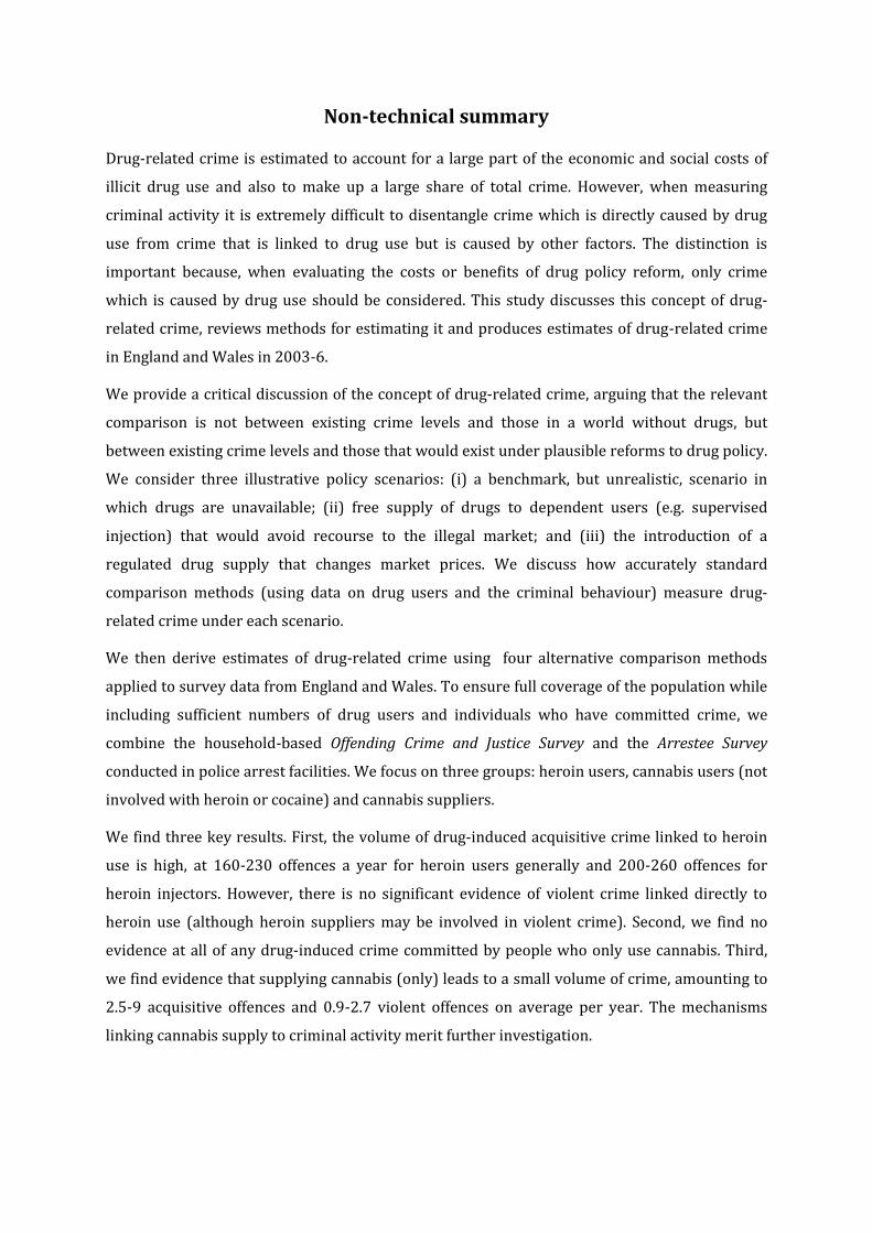
5.3 Self-assessed motivation for crime

The AS contains two questions on the motivation for crime: one asks for the proportion of the

respondent’s crimes that he or she has committed in order to pay for drugs; another asks for the

proportion of crimes committed whilst ‘high’ on drugs. Answers are categorical: “all”, “most”,

“some” or “none”; and, for quantitative analysis, we assume these equate to average proportions

100%, 67%, 33% and 0% respectively. The results are presented in Table 4 below. In most

cases, they are slightly smaller than the estimates of drug-induced crime produced by matching

methods in the AS sample (Table 3). Both suggest a lower level of drug-induced crime than the

naive estimates in Table 1 or Table 2. For heroin users, these estimates indicate that around

three-quarters of their acquisitive crime is attributable to drug use, but virtually none of their

violent crime. For cannabis users, a negligible (and mostly statistically insignificant) volume of

crime is attributed to drug use by the matching and self-assessment methods.

15

Table 5 Estimated drug-induced crime among arrestees: self-assessed motives ( )

Crime measure

Indicator of drug use Heroin injector

Heroin user

Positive opiates test

Cannabis-only user

Cannabis-only supplier

Crimes committed to buy drugs Annual number of shop thefts

158 (20.2)

174 (22.5)

140 (25.7)

3.63 (1.10)

32.8 (8.5)

Annual number of acquisitive crimes

224 (24.2)

245 (26.8)

197 (29.1)

10.5 (5.82)

96.1 (46.0)

Annual income from acquisitive crime

£7,162 (1,130)

£7,809 (1,222)

£7,007 (1,700)

£131 (33.7)

£1,881 (678)

Annual number of violent crimes

1.43 (0.58)

1.55 (0.64)

0.47 (0.13)

0.40 (0.13)

3.73 (1.16)

Crimes committed under the influence of drugs or to buy drugs Annual number of shop thefts

160 (19.6)

176 (21.8)

142 (25.6)

4.19 (1.11)

35.6 (8.49)

Annual number of acquisitive crimes

228 (23.3)

250 (25.7)

201 (28.8)

11.8 (11.1)

106 (44.9)

Annual income from acquisitive crime

£7,298 (1,142)

£7,943 (1,234)

£7,088 (1,695)

£160 (37.2)

£2,085 (671)

Annual number of violent crimes

1.54 (0.58)

1.64 (0.63)

0.58 (0.14)

0.50 (0.14)

4.47 (1.21)

6 Combined estimates

No one source of survey data is adequate for our purposes, and there are two alternative ways of

combining multiple datasets. One is to concatenate the OCJS and AS samples (using weights to

achieve the correct sample proportions) and then carry out estimation on the merged sample.

Another is to implement the estimates separately for the OCJS and AS samples and combine the

results. Under ideal conditions, the former approach is preferable, since the latter entails some

negative bias, essentially because an arrestee can never be matched to a non-offending non-

arrestee within the AS. But the ideal merged-survey approach only works if the appropriate set

of matching variables is observable in both the OCJS and AS surveys, and this is not the case in

practice. Differences in questionnaire content mean that merging the samples would only allow

matching on a reduced set of characteristics and it is doubtful whether this could adequately

16

deal with the confounding problem, leading to a substantial over-estimate of the true causal

impact of drug-use on crime. For this reason, we combine separate PATT estimates, but we first

consider the potential bias entailed and give an indication of its likely magnitude.

Consider a simple matching framework in which we estimate a PATT defined as:

(15)

where and are the crime levels that would be observed with drug use absent or present and

the outer expectation is with respect to the distribution of x in the drug-involved population.

Separating arrestees (a = 1) and non-arrestees (a = 0), the PATT can be written:

which can be re-expressed as:

where is the weighted PATT

conditional on arrest status, using weights , which adjust for

differences in the risk of arrest.

Equation (16) implies that the true PATT is a weighted combination of separate PATT constructs

for arrestees and non-arrestees, plus a bias term which is the expected value of the product of

two components: and

0, , =1 E 0| =0, , =0. These are respectively the difference in the probability of arrest for

drug-users and non-users and in the expected crime level for drug-free arrestees and non-

arrestees. Both are positive so combining separate PATT estimates from the OCJS and AS will

underestimate the scale of drug-induced crime to some degree.

We do not have a full set of covariates observable in both surveys, so the bias term cannot be

estimated exactly; nevertheless, there is some indication of the typical size of these terms. OCJS

estimates of the mean unconditional difference are 0.078

for heroin use, 0.026 for cannabis use and 0.005 for cannabis supply.2 Estimates of the mean

difference from AS and OCJS data are respectively 19.20,

8.34 and 42. 38 for the number of acquisitive crimes and 1.4, 0.6 and 0.9 for the number of

violent crimes.3 Multiplying these together,4 indicates a downward bias in the estimated annual

mean level of drug-induced crime of around 2 acquisitive crimes and 0.2 violent crimes for

2 Standard errors 0.055, 0.005 and 0.009 respectively 3 Standard errors1.29, 1.26 and 2.76 (acquisitive crimes) and 0.17, 0.19, 0.14 (violent crimes). 4 Note that , so we are assuming that the covariance over x of A and B is small.

17

heroin use; 0.2 acquisitive and 0.02 violent crimes for cannabis use; and 0.4 acquisitive and 0.01

violent crimes for cannabis supply. Given all the other estimation uncertainties, this does not

seem a cause for particular concern.

Without further information, the AS and OCJS are not sufficient because they do not tell us the

relative sizes of the household and non-household or arrestee and non-arrestee populations, and

they do not cover the non-arrestee, non-household population. We solve this coverage problem

with a mixture of assumption and further data. Population estimates from the Office for National

Statistics give an estimate of the relative size of the household and non-household populations,

but there is no available source of data on the non-arrestee, non-household population. Let

PATTA and PATTH,NA be the PATT estimates from the AS and non-arrestee subsample of the OCJS

data, respectively, giving the appropriate weighted average:

) (17)

where P( ), P(H, ) and P(NH, ) are the population proportions

of arrestees, of non-arrestees in the household sector and of non-arrestees in the non-household

sector, all conditional on drug use ( ). The PATT for the last of these groups is not

identifiable. If we assume a uniform PATT for non-arrestees in the household and non-

household populations, , definition (17) simplifies to:

(18)

and we then need only to know the population proportion of drug users who are arrestees,

P( ). Using the law of conditional probability, this is:

The AS, OCJS and ONS population statistics identify P( ), P( ) and P(H)

respectively. The arrest probability P( ) is P( |H)P(H)/P(H| ), whose three

components are identified by the OCJS, ONS and AS data respectively. The only term in (19)

which is not identified is the first term in the denominator, P( , |NH), which requires

evidence on non-arrestee members of the non-household population. This term makes a small

contribution to (19) since P(NH) is small, and it can be neglected with little loss of accuracy. We

assume that the proportion of drug-using non-arrestees is similar in the household and non-

18

household populations,5 so that we can write P( , |NH) P( , |H) and the

resulting approximation to the weight P( ) is:

Table 6 shows the components of the calculation of for four of the definitions of

drug status (note that bio-assay is not available for OCJS respondents). It is striking that the

probability of arrest conditional on drug status varies widely across forms of involvement with

drugs and that, for the two definitions of heroin user, it is so much higher than the arrest

probability in the general population.

Table 6 Population proportions

Parameter Estimate

(%) Standard error

Arrestee Survey: P(H | ) 91.4 (0.40) Population statistics: P(H) 94.1 (-) OCJS: P( | H) 1.07 (0.08) Combined: P( ) 1.09 (0.25)*

P( |d = heroin injector) 90.5 (4.76)* P( | d = heroin user) 65.6 (7.42)* P( | d = cannabis user) 4.99 (1.08)* P( | d = cannabis supplier) 6.14 (1.48)*

* Calculated using an assumed value of 0.2 for the standard error for P(H)

Table 7 shows the resulting estimates of the mean level of drug-related crime for people aged 17

and over in England and Wales, with one of four forms of involvement with drugs. They are

based on the propensity score estimates for the AS and OCJS samples and the weights reported

in Table 8, for three categories of acquisitive crime and for violent crime. For the criminal

income category, where no estimate is available for the OCJS, we have assumed average

proceeds of £30 per acquisitive crime for the non-arrestee population. The overall results are

below those estimated for the arrestee sample, because the rate of offending is so much lower in

the non-arrestee population. For acquisitive crime committed by self-reported heroin users,

they are about two-thirds the level reported by heroin-using arrestees alone; the difference is

much smaller for heroin injectors, who are almost absent from the OCJS sample. Drug-related

5 The report of the National Equality Panel (NEP 2010) suggests that there are currently around 0.85-0.9m members of the non-household population, of whom over half are in residential care homes and therefore very unlikely to be illicit drug users. The next largest group is people in armed forces accommodation (0.22m), which seems unlikely to have an especially high rate of drug use and non-arrest. In fact, the weight (22) is not very sensitive to the unknown

factor P( , |NH), which would have to be considerably larger than P( , |H) to make a significant difference to the calculation.

19

crime is estimated to be essentially zero among cannabis-only users as one might expect, and it

is very small for cannabis-only suppliers, generating proceeds of around £5 per week.

Table 7 Combined-data estimates of the PATT

Crime measure Indicator of drug use

Heroin injector

Heroin user

Cannabis-only user

Cannabis-only supplier

Annual number of shop thefts

161 (13.1)

135 (16.6)

0.25 (0.20)

0.77 (1.30)

Annual number of acquisitive crimes

231 (17.5)

191 (23.1)

0.45 (0.28)

5.75 (2.00)

Annual income from acquisitive crime

£6,760 (805)

£5,334 (795)

£4.77 (18.8)

£235 (102)

Annual number of violent crimes

-0.23 (0.55)

0.30 (0.47)

0.36 (0.23)

1.81 (0.55)

Note: Calculated using weights adjusting for sample design, non-response and arrest frequency. Standard errors in parentheses, calculated allowing for stratified and clustered sample design where possible.

7 Consistency with experimental evidence

There is no possibility of a direct controlled experiment involving the permanent removal of

illicit drug availability, but there have been many experiments that evaluate interventions

intended to reduce consumption of illegally-supplied drugs. Most of these experiments involve

either the prescription of substitute drugs (primarily methadone) or direct prescription of

opiates (usually injectable heroin or morphine). Substitutes are generally provided at little or no

cost and can therefore be expected to reduce the demand for “street” drugs and consequently

reduce the need for income-generating crime. These experiments are all conducted within the

context of a drug treatment programme, so the effect of access to low-cost, high-quality heroin is

necessarily confounded with the impact of the associated treatment. For this reason, we

generally observe reductions in illicit drug use in the control groups that receive no heroin, as

well as the treatment groups that do. This confounding makes it difficult to identify drug-

induced crime directly from the experimental evidence.

Table 8 summarises recent experiments from six different countries, involving supervised

injection of heroin for treatment-resistant drug users. As pointed out in a recent Cochrane

review (Ferri et al 2006) and Rowntree survey (Stimpson and Metrebian 2003), these studies

are not fully comparable in terms of observed outcomes and treatments. From a social welfare

perspective, there are particular weaknesses in terms of their measurement of criminal activity

as an outcome and their short durations. The experiments all provided randomly-selected

20

subsets of participants with high-quality injectable heroin in (average) doses ranging from

275mg to 548mg per day at zero or greatly reduced cost (but subject to the additional costs of

attending the experimental site). The experiments were all driven by medical concerns and the

published findings generally provide little information about the economic circumstances of the

subjects or the net relative costs that they faced for ‘street’ and prescribed heroin.

All experiments recorded the observed impact on various outcomes, but particularly on health

indicators and continued use of illicit heroin (measured through self report and/or biomarkers).

Impacts were inferred either from comparisons of post-treatment levels in the treatment and

control groups (“differences-in-levels”) or by comparing differences between pre- and post-

treatment outcomes for the control and treatment groups (“differences-in-differences”).

The theoretical analysis of section 2.3 suggests that matching methods tend to overestimate the

impact on crime of a heroin prescription programme that is not able to prevent all resort to the

illicit market. All the experiments summarised in Table 10 reported large falls in the use of street

heroin, ranging from 66% (Spain) to 85% (Germany) in terms of days use per month; abstinence

rates rose from zero at baseline to 33% (Geneva) or 37/51% (England), the latter depending on

measure used. These findings confirm what we would expect from basic consumer theory: that

the provision of fixed supplies of a commodity at a zero or subsidised price will reduce the

consumption of a close substitute (street heroin). Nevertheless, use of street heroin remained

significant in almost all experiments, underlining the need for caution in applying external

estimates of drug-related crime to projected interventions of this kind.

There is evidence of a reduction in acquisitive crime accompanying the reductions in the cost of

heroin consumption brought about by the experiments, but it is hard to draw firm conclusions

about the magnitude of the effect. There is little consistency in the recording and analysis of

crime outcomes across the studies and those that do report impacts on the volume of criminal

activity suggest an effect ranging from 44% (Canada) to 99% (Spain), although the substantial

decreases observed also in the control groups suggest that much of this may be due to other

aspects of the treatment programme. Our survey-based estimates suggest that around 75% of

property crime committed by heroin users is drug-related. The experimental evidence certainly

spans this figure, but the wide range of results prevents any firm conclusion being reached.

There are two major issues to bear in mind when comparing survey and experimental estimates.

First, our analysis rests on a combination of OCJS and AS samples, with forms of random

sampling used within their target populations and weighting used to adjust for selection into

those populations. In contrast, convenience sampling is the primary method for recruiting

experimental participants, who are screened in various ways. Past treatment failures and

cooperation with an intensive treatment programme are requirements of participation and no

21

adjustment is made for refusal and other forms of non-response. These selection processes

result in experimental groups with quite different characteristics than those of drug users

generally – indeed, that is a deliberate feature of their design. Second, the effect of the

accompanying psychosocial treatment (counselling, education, etc) in the experimental cases

may modify the response that would be induced by the provision of low-cost heroin alone. We

would expect treatment to amplify the tendency for crime to be reduced by the heroin

intervention, so the true figure is somewhere below the total reported difference between

baseline and end-of-treatment levels of criminal activity.

To summarise, we can say that, given the wide range of experimental estimates and the

uncertainties involved in comparing survey-based and experimental estimates, there is no

demonstrable inconsistency between the survey and experimental evidence on the extent of

drug-induced crime.

22

Table 8 Evidence from European heroin injection experiments

Time and place Intervention Pre- and post-treatment illicit

drug use Crime outcome measure Effect size

Switzerland (Uchtenhagen et al 1999): 15 cities, 1994-6

1035 heroin addicts in treatment, assigned to various experimental treatments mostly without randomised controls. 18 months duration. Some patients were required to pay a contribution to programme costs.

81% prevalence of daily illicit heroin use pre-treatment 6% after 18 months. Significant decrease also for cocaine consumption but not cannabis.

(i) Court convictions 80% decrease (ii)Police-recorded offences

70% decrease in no. of offences

(iii) Self-reported offences 60% decrease in prevalence (iv) % income from illegal sources

fall from 69% to 10%

Switzerland (Perneger et al 1998): Geneva 1995-6

51 heroin addicts in poor health with at least two past treatment failures, recruited in outpatient clinic. Treatment group received average of 480 mg intravenous heroin per day for 6 months and were required to give up driving. Control group received various other treatments, mainly methadone maintenance.

Treatment group: 100% daily street heroin use pre-treatment 4% daily / 19% occasional use post-treatment Control group: 90% daily / 10% occasional pre-treatment 48%, 19% post-treatment

(i) Pre-post treatment difference in criminal charges for acquisitive crime (ii) Pre-post treatment difference in criminal charges for violent crime (iii) Pre-post treatment difference in income from non-drug illicit income

-86% and +50% for treatment and control groups -67%, 0% for treatment and control groups -65%, +70% for treatment and control groups

Netherlands (van den Brink et al 2003, Dijkgraaf et al 2005): 6 cities: 1998-2000

549 heroin addicts participating unsuccessfully in methadone maintenance programmes (339 full compliers). 5 treatment groups received combinations of methadone and inhalable or injectable heroin (mean dose 548mg per day, within a maximum of 1000mg)

Not reported

(i) Mean days property crime during year (ii) Mean prosecutions for property crime / prostitution during year (iii) Mean prosecutions for violent crime

-61% difference-in-levels (10.3 v 37.5 days) -43% difference-in-levels (0.45 v 0.79 prosecutions) -88% difference-in-levels (0.02 v 0.16 prosecutions)

Germany (Haasen et al 2007): 7 cities, 2002-3

1015 heroin users with poor response to current treatment or who were not in treatment for at least 6 months. Comparison of 8 randomised groups differing in medication (injected heroin/oral methadone) and psychosocial care (education/case management). Study duration was 12 months (mean daily heroin dose 442mg)

Fall in use of illicit heroin: 85% (23 3 days per month), 65% (23 8 days) for treatment and control groups. Difference-in-levels for prevalence of positive urine tests for street heroin at 12 months: 18% (treatment), 30% (control). All figures approximate.

Not reported

23

Table 8 continued

Time and place Intervention Pre- and post-treatment

illicit drug use Crime outcome measure Effect size

Spain (March et al 2006): Granada, 2003-4

62 opioid-dependent subjects (44 full compliers) recruited in drug-dealing areas and through treatment contacts. All had 2 or more failed past spells of methadone treatment. Control group received methadone only; treatment group methadone + twice-daily injected heroin (average 275 mg. per day) and methadone (43mg.). All had access to social, legal, psychiatric & medical support. 9 month duration.

Use of street heroin fell by 66% (24.58.3 mean days per month) for the treatment group; and by 27% (23.316.9 days) for the control group.

Difference in mean no. of days’ illegal activity in last month at baseline and at 9 months

99% decrease (11.50.6 days) for treatment group; 49% decrease (8.04.1 days) for control group

Canada (Oviedo-Joekes et al 2009): Montreal and Vancouver, 2005-8

226 heroin injectors with at least two past treatment failures. Control group received oral methadone (average dose 96mg.). The treatment group received injectable heroin (average daily dose 392mg.). Both groups also received psychosocial and primary care services. 12 months study duration.

No. days illicit heroin last month fell by 80% (26.6 5.3) for treatment group; 56% (27.4 12.0) for control group. Reductions in median spending were 73% ($1,200$320 p.m.) for treatment group and 67% ($1,200$400) for control group. No change in illicit cocaine use.

(i) Proportion with reduction in non-drug crime over treatment period (ii) Pre-/post-treatment difference in mean EuroASI subscale for illegal activities

44% (treatment group); 34% (control group) -46% (treatment group); -34% (control group)

UK (Lintzeris et al 2006; Strang et al 2010):Brighton, Darlington, London, 2005-8

127 long-term heroin injectors with continuing use of illicit heroin despite at least 6 months’ oral methadone treatement. Treatment groups received (A) oral+injected methadone or (B) injected heroin+oral methadone. Control group (C) received oral methadone.

Urine tests: 37% of heroin group B, 18% (group A), 8% (group C) tested negative for street heroin in weeks 23-26. Self report: 51% (B), 19% (A), 17% (C) reported abstinence from street heroin.

Not reported

24

8 The social cost of drug-induced crime

Crime involves a number of distinct costs and benefits to different parties. For example, a

domestic burglary imposes a cost on the victim including the value of the goods lost and the cost

of making good any damage caused by entry. Some of those losses may be met by household

insurance, but there is a cost in acquiring that insurance cover and negotiating the claim. There

may be further intangible costs in the form of psychological distress, which may persist in the

form of an increased future fear of crime. Society as a whole bears a cost in the form of the

policing and criminal justice response to the crime and possibly also health care costs if the

burglary involved psychological or physical injury to the victim which prompted a response

from the health care system. Society also bears some additional intangible costs from the social

malaise that is caused by crime, particularly in certain neighbourhoods. Property crime also

involves a transfer of resources. The criminal benefits from the income he or she gains from

reselling the stolen property or using any stolen property that is retained. The dealer who

handles the stolen goods profits from the transaction and the ultimate purchaser benefits from

the opportunity to buy low-cost goods. These transfer benefits are almost never included in

social cost accounting of crime, which normally rests on an unstated assumption that theft is

pure economic loss, equivalent to total destruction of the stolen property.

It is difficult to put values on all these cost-benefit elements, even for financial costs, since the

reporting or recording of the financial value of crime by victims (in surveys like the British

Crime Survey), by criminals (in surveys like the OCJS and AS), and by agencies like the police and

insurance companies are subject to wide margins of error, which are themselves not easy to

estimate. However, some estimates do exist and we exploit these to construct a variable to

represent at least part of the social cost of the crime reported by respondents to the AS and OCJS,

which allows us to repeat the analysis of section 5 in social cost terms. The cost assumptions

underlying construction of this variable are set out in Table 9. They are based, as far as possible,

on the semi-official analysis by Dubourg et al (2005), which updates and improves upon the

earlier costings of Brand and Price (2000). However, the more recent cost estimates only apply

to crime against private individuals and households and excludes losses to commercial

organisations. We therefore use a combination of the two sources. Table 11 also shows the cost

estimates used by the official Drug Harm Index (MacDonald et al 2005). The estimates from

Dubourg et al (2005) includes tangible costs (‘defensive expenditures’, insurance

administration, value of property stolen or damaged, lost output, health and other services to

victims, and policing and criminal justice costs) and also intangible costs (physical and

emotional impact on the direct victims). The last category of costs is extremely important, since

it makes up about half of the total social cost of crime against personal sector victims, but is

25

particularly difficult to value, with alternative methodological approaches giving widely differing

results (Dolan et al 2005). The Dubourg et al estimates of intangible costs are based on quality-

adjusted life years (QALYs), as used extensively in the evaluation of health interventions. To

emphasise the large uncertainties involved in these cost estimates, Table 9 gives the unit costs

we adopt for our calculations in rounded form to avoid spurious precision and we also give our

own subjective indication of the range of uncertainty associated with them. They should not be

interpreted as confidence intervals, since they reflect conceptual ambiguity at least as much as

statistical error. Note also that there is some mismatch between the crime categories of Table 9

and those used in our analysis of AS and OCJS data. For example, the ‘semi-licit’ categories of

begging and prostitution are excluded from Table 9 and thus are implicitly assumed to entail

social costs equal to those of the average acquisitive crime.

Table 9 Assumed unit social costs of crime (2003 prices)

Crime category

Central estimate of

unit cost

Range of

uncertainty

Sources

BP2000a DHT2005b DHI2005c

Shop theft 110 80-140 110 70.54

Other non-vehicle theft 634 434-834 - 634 375

Theft of vehicle 5000 4500-5500 _______ 4924 d_______ 5900

Theft from vehicle 850 600-1000 _______ 848 d _______ 568

Domestic burglary 3250 2750-3750 - 3268 2535

Non-domestic burglary 3000 2500-3500 2976 - 2976

Personal robbery 7250 6750-7750 - 7282 5180

Shop robbery 5500 4500-6500 5511 - -

Fraud 1600 1000-2200 1653 - -

Personal robbery 7250 6750-7750 - 7282 5180

Shop robbery 5500 5000-6000 5511 - -

Assault & wounding 3120 2600-3640 - 1440 / 8852 e -

Notes: Gross external costs (£ per offence in 2003 prices), including tangible and intangible costs to victims and tangible costs to society in general (not net of benefit to criminals). a Brand and Price (2000) b Dubourg et al (2005) c Drug harm Index: MacDonald et al (2005) d Composite of/from theft of private vehicles (DHT2005) and commercial vehicles (BP2000) e Common assault and wounding, respectively.

We attach a social cost to estimates of drug-related crime by applying the average unit cost

figures for acquisitive and violent crime to the PATT estimates in Table 7 for each category of

drug user. Note that the acquisitive and violent crime categories overlap, because personal and

shop robbery is common to both, so it is not strictly possible to sum them to obtain an aggregate

figure for acquisitive and violent crime. The results are presented in Table 10, with indicative

26

ranges of uncertainty, constructed by combining the sampling error confidence intervals from

Table 7 with the subjective uncertainty indicators from Table 9 by treating the latter as if they

were normal 90% intervals. Although the arithmetic of confidence intervals is used to construct

the ranges of uncertainty quoted in Table 10, they should be interpreted as largely subjective.

Table 10 Estimated per capita external social cost of drug-related crime

Crime measure Indicator of drug use

Heroin injector

Heroin user

Cannabis-only user

Cannabis-only supplier

Acquisitive crime per user 85.3 [68.5 , 102.1]

80.0 [60.7 , 99.3]

0.3 [-0.01 , 0.6]

3.9 [1.6 , 6.2]

Violent crime per user -1.6 [-8.1 , 4.8]

2.1 [-3.4 , 7.6]

2.6 [-0.1 , 5.3]

12.8 [6.3 , 19.2]

Group size (‘000) 53.8 (35.0 , 72.6)

76.9 (55.3 , 98.5)

2,467 (2,342 , 2,592)

212 (177 , 247)

Aggregate social cost: acquisitive crime (£bn)

4.587 [2.437 , 6.737]

6.153 [3.585 , 8.720]

0.747 [-0.024 , 1.518]

0.829 [0.318 , 1.341]

Aggregate social cost: violent crime (£bn)

-0.088 [-0.438 , 0.261]

0.164 [-0.262 , 0.591]

6.346 [-0.345 , 13.04]

2.710 [1.273 , 4.148]

Note: Ranges of uncertainty in square brackets are indicative only and should not be interpreted as conventional confidence intervals.

The estimated social cost of drug-related crime caused by heroin use is high, probably in the

range £65,000-100,000 per user. There is no detectable external cost in terms of crime imposed

on society by those who use cannabis alone, but cannabis dealing appears to bring with it a

significant level of mainly violent crime in the range £6,000-£20,000 per head, the greater part

of which is in the form of assault of various kinds, rather than property-motivated robbery.

We estimate the size of each group of drug users as N P( )P( )/P( ),

where N is the size of the England and Wales 17-65 population. Table 12 gives estimates of these

numbers and the implied aggregate social costs, together with indicative ranges of uncertainty.

The results suggest that the external social costs of acquisitive crime caused by current heroin

use among the adult population in England and Wales amount to £3.6-8.7bn, of which £2.4-6.7bn

is attributable to heroin injectors. Although there is a large point estimate for the aggregate

social cost of violent crime caused by cannabis use, this is due to the large size of this group and

the very high unit social cost assigned to violent crime. In fact there is no statistically significant

evidence of any crime induced by cannabis use, which is reflected in the huge range of

uncertainty spanning zero. A modest aggregate social cost of drug-related acquisitive (£0.3-

1.3bn) and violent crime (£1.3-4.1bn) is attributed to cannabis suppliers. To put these figures in

perspective, the NHS disease costs associated with tobacco smoking in England in 2006 have

27

been variously estimated as £2.7bn (Callum et al 2011) and £5.2bn (Allender et al 2009) and in

Wales in 2007/8 as £0.39bn (Phillips and Bloodworth 2009).

9 Conclusions

We have focused particularly on three groups of people who are of particular interest in terms of

drugs policy: (i) heroin users, because of the possibly high external cost their drug use imposes

on society; (ii) users of cannabis who are not currently involved with heroin or cocaine, because

of the high prevalence of cannabis consumption; and (iii) people involved in the supply of

cannabis (only), because of their possibly high risk of transition into hard drug supply. Our aim

was to estimate the magnitude of one component of the external social cost of drug use for these

three groups – the additional property crime and violent crime which is causally linked to their

involvement with illicit drugs. There are five main conclusions.

First, we find that the volume of drug-induced property crime linked to heroin use is high, but

there is no significant evidence of violent crime linked directly to heroin use (this is not to say

that there is no violent crime caused by heroin suppliers). The average level of acquisitive crime

is probably in the range of 160-230 offences a year for heroin users generally, and rather more

for heroin injectors (200-260 offences). Around 70% of these offences are episodes of shop theft.

This criminal activity generates an income for the users estimated to be £4,000-6,700 a year

(£5,500-8,000 for injectors). The cost imposed on society by heroin users’ drug-induced crime is

extremely high if we include an allowance for the distress as well as tangible losses experienced

by victims and for the costs of reactive policing and criminal justice procedures. These social

costs are highly uncertain, but we suggest that the annual social cost caused by an average

heroin user is in the range £60,000-100,000, implying an aggregate cost from all (adult) heroin

users in England and Wales in the range £3.5-10.5bn. There is no obvious conflict between these

estimates and the results of various national heroin-injection experiments which have had the

effect of greatly reducing resort to the market for expensive street heroin.

A second important finding is that there is no evidence at all of any drug-induced crime

committed by people who use cannabis alone. This contradicts perceptions held by many of the

general public: in a survey carried out by the Advisory Council on the Misuse of Drugs (2008,

Table 6), two-thirds of those interviewed “tended to agree” or “strongly agreed” with assertions

that cannabis use contributes to social disorder or to an increase in criminal activity.

Third, we find evidence of only a small volume of crime causally related to the activity of people

involved in supplying (only) cannabis. This amounts to 2.5-9 acquisitive offences and 0.9-2.7

violent offences on average per year, with associated external social cost of £1,700-£6,400

(acquisitive) or £6,400-£19,300 (violent). Violent crime is sometimes a feature of drug supply so

the latter result is unsurprising, but the interpretation of the finding on acquisitive crime is not

28

clear. Drug supply is often a source of income for drug users, so cannabis dealing could

substitute for acquisitive crime rather than increase it. One possibility is that cannabis supply is

acting here as a proxy for a particularly intensive level of cannabis use, which might be funded

by a mixture of property crime and dealing activity. This merits further investigation.

A fourth conclusion relates to the available evidence base. Quantitative research on drug-related

crime should be based on survey evidence that adequately represents population groups with

high rates of offending and drugs use, and which makes it possible to address the difficult

problems involved in identifying causal relationships. The ideal source of evidence would be a

large-scale longitudinal survey representative of both the household and non-household

resident populations. No such survey exists or is ever likely to exist, and we have used instead a

composite multi-survey cross-section approach using matched comparison methods to estimate

causal links. This was only possible because we have a targeted survey (the Arrestee Survey) of

offending and drug use which covers both drug-using and non-drug-using offenders, and a

general-population survey (the Offending Crime and Justice Survey) which also covers both

offending and drug use. Both surveys were ended by the Home Office in 2006 and, to the best of

our knowledge, there currently exist no surveys for England and Wales that would allow an

updated analysis of this kind to be undertaken. Current Home Office surveys fail to cover both

offending and drug use (for example, the British Crime Survey does not ask about respondents’

own criminal activity, and the DTORS/NTORS treatment cohorts select only drug users and

therefore offer no comparison with non-users).

The study is also significant on a theoretical and methodological level. We have shown that, in a

context where both the ‘treatment’ and its ‘outcome’ are the result of individual choice, there is a

link between the validity of statistical methods based on matching ‘treatment’ and ‘control’ cases

and the assumption of separable preferences, giving a new rationale for the use of matching

methods in settings where causality is a particularly difficult issue. We have also extended

matching methods to settings which require a combination of endogenously-selected data

sources to achieve adequate population coverage.

References

Abadie A. and Imbens, G. (2006). Large sample properties of matching estimators for average treatment effects, Econometrica 74, 235-267.

Advisory Council on the Misuse of Drugs (2008). Cannabis: Classification and Public Health. London: Home Office.

Allender, S., Balakrishnan, R., Scarborough, P., Webster, P. and Rayner, M. (2009). The burden of smoking-related ill health in the UK, Tobacco Control 18, 262-267.

Bennett, T. and Holloway, K. (2009). The causal connection between drug misuse and crime, British Journal of Criminology 49, 513-531.

29

Boreham, R., Fuller, E., Hills, A. and Pudney, S. E. (2006). The Arrestee Survey Annual Report: Oct 2003 – Sept 2004. England and Wales. London: Home Office Statistical Bulletin 04/06.

Burr, A. (1987). Chasing the dragon: heroin misuse, dependency and crime in the context of South London culture, British Journal of Criminology 27, 333-357.

Brand, S. and Price, R. (2000). The economic and social costs of crime. London: Home Office Research Study 217.

Callum, C., Boyle, S. and Sandford, A. (2011). Estimating the cost of smoking to the NHS in England and the impact of declining prevalence. Health Economics, Policy and Law 6, 489-508.

Caulkins, J. P. and Reuter, P. (1998) What Price Data Tell Us about Drug Markets, Journal of Drug Issues, 28: 593-612, Summer 1998.

Chimeli, A. B. and Soares, R. R. (2011). The use of violence in illegal markets: evidence from mahogany trade in the Brazilian Amazon. Bonn: IZA Discussion Paper 5923.

Clements, K. W. and Zhao, X. (2005). Economic aspects of marijuana, mimeo, University of Western Australia.

Collins, D. J. and Lapsley, H. M. (2008). The costs of tobacco, alcohol and illicit drug abuse to Australian society in 2004/05. Canberra: Commonwealth of Australia.

D’Amico, E. J., Edelen, M. O., Miles, J. N. V. and Morral, A. R. (2008). The longitudinal association between substance use and delinquency among high-risk youth, Drug and Alcohol Dependence 93, 85-92.

Day, C.,Topp, L., Rouen, D., Darke, S., Hall, W. and Dolan, K. (2003). Decreased heroin availability in Sydney in early 2001, Addiction 98, 93-95.

Dolan, P., Loomes, G., Peasgood, T. and Tsuchiya, A. (2005). Estimating the intangible victim costs of violent crime, British Journal of Criminology 45, 958-976.

Dolan, P. and Peasgood, T. (2006). Estimating the economic and social costs of the fear of crime, British Journal of Criminology 47, 121–132.

Dubourg, R., Hamed, J. and Thorns, J. (2005). The economic and social costs of crime against individuals and households 2003/4. London: Home Office online report 30/05.

Ferri, M., Davoli, M. and Perucci, C. A. (2006). Heroin maintenance treatment for chronic heroin dependent individuals: a Cochrane systematic review of effectiveness, Journal of Substance Abuse Treatment 30, 63-72.

Fischer, B., Medved, W., Kirst, M., Rehm, J. and Gliksman, L. (2001). Illicit opiates and crime: results of an untreated user cohort in Toronto. Canadian Journal of Criminology 43, 197-217.

Godfrey, C., Eaton, G., McDougall, C. and Culyer, A.(2002). The economic and social costs of class A drug use in England and Wales. London: Home Office Research Study 249.

Goldstein, P. (1985). The drugs/violence nexus: a tripartite conceptual framework, Journal of Drug Issues 15, 493-506.

Haasen C., Verthein U., Degkwitz P., Berger J., Krausz M., Naber D. (2007). Heroin-assisted treatment for opioid dependence: randomised controlled trial, British Journal of Psychiatry 191, 55-62.

Hales, J., Nevill, C., Pudney, S. E. and Tipping, S. (2009). Longitudinal analysis of the Offending Crime and Justice Survey 2003-6. London, Home Office: Online Research Report 19.

Hammersley, R., Forsyth, A., Morrison, V. and Davies, J. B. (1989). The relationship between crime and opioid use, British Journal of Addiction 84, 1029-1043.

Hoaken, P. N. S. and Stewart, S. H. (2003). Drugs of abuse and the elicitation of human aggressive behavior, Addictive Behaviors 28, 1533-1554.

Jones, A., Donmall, M., Millar, T., Moody, A., Weston, S., Anderson, T., Gittins, M., Abeywardana, V. and D’Souza, J. (2009) The Drug Treatment Outcomes Research Study: Final outcomes report. London: Home Office Research Report 24.

Phillips, C. and Bloodworth, A. (2009). Cost of Smoking to the NHS in Wales, ASH Wales/ BHF Cymru.

30

Stevens, A., Trace, M. and Bewley-Taylor, D. (2005). Reducing drug related crime: an overview of the global evidence. Oxford: The Beckley Foundation.

Stewart, D., Gossop, M., Marsden, J., and Rolfe, A. (2000). Drug misuse and acquisitive crime among clients recruited to the National Treatment Outcomes Research Study. Criminal Behaviour and Mental Health 10, 10-20.

Leuven, E. and Sianesi, B. (2003). PSMATCH2: Stata module to perform full Mahalanobis and propensity score matching, common support graphing, and covariate imbalance testing. http://ideas.repec.org/c/boc/bocode/s432001.html (version 4.0.4)

MacDonald, Z., Tinsley, L., Collingwood, J., Jamieson, P., Pudney, S. E. (2005) Measuring the Harm from Illegal Drugs using the Drug Harm Index. London: Home Office Online Report 24/05.

MacDonald, Z., Collingwood, J., and Gordon, L. (2006) Measuring the Harm from Illegal Drugs using the Drug Harm Index – an Update. London: Home Office Online Report 08/06.

March J.C., Oviedo-Joekes E., Perea-Milla E., Carrasco F., PEPSA team. (2006). Controlled trial of prescribed heroin in the treatment of opioid addiction, Journal of Substance Abuse Treatment 31(2), 203-211.

Mayer, P. and Höllt, V. (2005). Genetic disposition to addictive disorders: current knowledge and future perspectives, Current Opinion in Pharmacology 5, 4-8.

Miron, J. (1999). Violence and the US prohibitions of drugs and alcohol, American Law and Economics Review 1, 78-114.

National Equality Panel (2010). An Anatomy of Economic Inequality in the UK: Report of the National Equality Panel. London School of Economics and Political Science: CASE report 60.

ONDCP (2004). The Economic Costs of Drug Abuse in the United States 1992-2002. Washington DC: Executive Office of the President (publication no. 207303).

Oviedo-Joekes E., Brissette S., Marsh D.C., Lauzon P., Guh D., Anis A., Schechter M.T. Diacetylmorphine versus methadone for the treatment of opioid addiction, New England Journal of Medicine 361(8), 777-86.

Perneger T.V., Giner F., del Rio M., Mino A. (1998). Randomised trial of heroin maintenance programme for addicts who fail in conventional drug treatments, British Medical Journal 317(7150), 13-18.

Pudney, S. E. (2003). The road to ruin? Sequences of initiation to drugs and crime in Britain, Economic Journal 113, C182-C198.

Rosenbaum, P.R. (2002). Observational Studies (2nd edition). New York: Springer

Rosenbaum, P.R. and Rubin, D.B. (1983). The central role of the propensity score in observational studies for causal effects", Biometrika 70, 41-55.

Rubin, D.B. (1980). Bias Reduction Using Mahalanobis-Metric Matching, Biometrics 36, 293-298.

Strang, J., Metrebian, N., Lintzeris, N., Potts, L., Carnwath, T., Mayet, S., Williams, H., Zador, D., Evers, R., Groshkova, T., Charles, V., Martin, A. and Forzisi, L. (2010). Supervised injectable heroin or injectable methadone versus optimised oral methadone as treatment for chronic heroin addicts in England after persistent failure in orthodox treatment (RIOTT): a randomised trial, The Lancet 375, 1885-1895.

Stimpson, G. V. and Metrebian, N. (2003). Prescribing heroin. What is the evidence? York: Joseph Rowntree Foundation.

Uchtenhagen, A., Gutzwiller, F., Dobler-Mikola, A., Steffen, T. and Rihs-Middel, M. (1999). Medical Prescription of Narcotics (vol. 1). Basel: Karger.

van den Brink W., Hendriks V.M., Blanken P., Koeter M.W., van Zwieten B.J., van Ree J.M. (2003) Medical prescription of heroin to treatment resistant heroin addicts: two randomised controlled trials, British Medical Journal 327(7410), 310-315.

Van Ours, J. C. and Williams, J. (2005). Cannabis prices and dynamics of cannabis use, Tilburg University: CentER Discussion Paper no. 2005-52.

Appendix: further tables

Table A1 Measures of drug use and crime: Arrestee Survey 2003-6

Indicator Definitions Sample nos. of users and

non-users

Sample prevalence

(%)

Heroin injector

Users: self-reporting both injecting drugs and heroin use in last month Non-users: all with valid responses to injecting and heroin questions

19,545 13.0

Heroin user Users: self-reporting heroin use in last month Non-users: all with valid responses to heroin questions

18,998 13.4

Positive screening test for opiates

Users: positive saliva screening test result for heroin or morphine Non-users: all providing testable saliva sample

14,174 15.5

Cannabis-only user

Users: self-reporting use of cannabis but no use of heroin, cocaine, crack or methadone in the last month Non-users: all with valid responses to drug questions, who report no use of heroin, cocaine, crack or methadone in the last month

12,744 32.8

Cannabis-only supplier

Users: self-reporting selling cannabis in last month but no selling of any other drug Non-users: all with valid responses to cannabis supply question, who report no selling of any other drug in the last month

13,237 3.5

Indicator Definitions No. of valid responses

Sample mean

Annual number of shop thefts

Self-reported number of shop thefts in last 4 weeks 13

17,721 34.5

Annual number of acquisitive crimes

Self-reported number of episodes during relevant reference period of: shop theft, begging, handling stolen goods, prostitution, controlling prostitution, vehicle theft, thefts from vehicles, domestic and other burglary, personal and shop robbery, theft from the person, financial and benefit fraud; converted to annual basis.

17,158 57.4

Annual income from acquisitive crime

Self-reported summed annual net income from acquisitive crimes, with follow-up check on the total

18,770 £2,222

Annual number of violent crimes

Self-reported number of episodes during relevant reference period of: personal and shop robbery and assault, converted to annual basis.

19,183 2.0

Table A2 Measures of drug use and crime: Offending, Crime and Justice Survey 2003-6

Indicator Definitions

Sample nos. of

users and non-users

Sample prevalence

(%)

Heroin user Users: self-reporting heroin use in last month Non-users: all with valid responses to heroin questions

15,483 0.17

Cannabis-only user

Users: self-reporting use of cannabis but no use of heroin, cocaine or crack in the last month Non-users: all with valid responses to drug questions, who report no use of heroin, cocaine or crack in the last month

14,942 9.29

Cannabis-only supplier

Users: self-reporting selling of non-class A drugs in last month but no selling of class A drugs Non-users: all with valid responses to non-class A supply question, who report no selling of class A drugs in the last month

15,460 0.90

Indicator Definitions No. of valid responses

Sample mean

Annual number of shop thefts

Self-reported number of shop thefts in last year 15,526 0.064

Annual number of acquisitive crimes

Self-reported occurrence of benefit fraud in last year and numbers of episodes of: shop theft, vehicle theft, thefts from vehicles, domestic and other burglary, personal and shop robbery, theft from the person.

15,219 0.112

Annual number of violent crimes

Self-reported number of episodes during last year of: personal and shop robbery and assault.

15,306 0.377

Table A3 Characteristics used for matching: AS and OCJS 2003-6

Sample mean or prevalence (%)

[standard error] Definition AS1 OCJS2

Age at time of interview 30.7 [1.7] 30.8 [0.1] Female respondent 16.4 [0.5] 49.9 [0.5] Has been in foster care 16.2 [0.5] 1.2 [0.1] Age at first arrest 20.9 [0.2] - Ever used cannabis 68.8 [0.6] 38.3 [0.5] Age at first use of cannabis (if ever used cannabis) 15.8 [0.1] 17.6 [0.1] Left school before age 16 34.3 [0.8] 12.4 [0.3] Was excluded from school 38.0 [0.7] 3.2 [0.2] Had difficulty with computer when using CASI 17.6 [0.5] 8.5 [0.3]

Note: 1 Means calculated using weights adjusting for sample design, non-response and arrest frequency. Standard errors calculated allowing for stratified and clustered sample design. 2 Means calculated using weights adjusting for sample design and non-response.