Drug Firms’ Payments and Physicians’ PrescribingBehavior in Medicare Part D

Colleen CareyCornell University

and NBER

Ethan M.J. LieberUniversity of Notre Dame

and NBER

Sarah MillerUniversity of Michigan

and NBER ∗

February 2020

Abstract

In a pervasive but controversial practice, drug firms frequently make monetary orin-kind payments to physicians in the course of promoting prescription drugs. We usea federal database on the universe of such interactions between 2013 and 2015 linkedto prescribing behavior in Medicare Part D. We account for the targeting of paymentswith fixed effects for each physician-drug combination. In an event study, we showthat physicians increase prescribing of drugs for which they receive payments in themonths just after payment receipt, with no evidence of differential trends betweenpaid and unpaid physicians prior to the payment. Using hand-collected efficacy dataon three major therapeutic classes, we show that those receiving payments prescribelower-quality drugs following payment receipt, although the magnitude is small andunlikely to be clinically significant. In addition, we examine five case studies of majordrugs going off patent. Physicians receiving payments from the firms experiencing thepatent expiry transition their patients just as quickly to generics as physicians who donot receive such payments.

JEL codes: I11 (Analysis of Health Care Markets); L15 (Information and ProductQuality); D83 (Search; Learning)

∗We are grateful for helpful comments from Judy Hellerstein, Seth Freedman, Sean Nicholson, AshleySwanson, Benedic Ippolito, Thuy Nguyen, and seminar participants at Harvard University, Cornell Univer-sity, University of Michigan, Duke University, Johns Hopkins University, University of Maryland, the 2020American Economic Association meetings, the 2015 International Health Economics Association meetings,the 2015 American Health Economics Conference, the 2016 Association for Public Policy Analysis and Man-agement Annual Meeting. Anup Das provided excellent research assistance. Colleen Carey acknowledgesthe financial support of the Robert Wood Johnson Foundation.

1

1 Introduction

More than 85 percent of drug firms’ marketing expenditures are targeted at influencing physi-

cians as the key prescribing decision-maker (Pew Charitable Trust, 2013). Such marketing

expenditures include face-to-face “detailing” visits from pharmaceutical sales representatives

that commonly involve purchases of food and beverage for physicians, as well as high-dollar

speaking fees or travel reimbursements. These financial interactions are commonly thought

to distort physician’s prescribing decisions; Consumer Reports declares that “a major con-

flict of interest is at work when a physician has accepted payments from a drug company

whose products he or she then prescribes” (Consumer Reports, 2014). However, the fact that

drug firms target payments at physicians who are ex ante most likely to prescribe the drug

makes it difficult to establish the causal effect of payments. In addition, even if payments

influence a physician’s behavior, it is an empirical question whether patients’ outcomes are

helped or harmed. Defenders of the practice argue that payments facilitate education on a

fast-changing evidence base: “Pharma reps provide timely access to balanced, FDA-approved

research and information. This ‘delivery mechanism’ organically complements and reinforces

the information they receive from medical journals and conferences” (Flewell, 2006).

In this paper, we use rich microdata to evaluate how financial interactions between drug

firms and physicians affect prescribing outcomes such as expenditures, the number of patients

taking the drug, transitions to generic versions of branded drugs, and the quality of prescribed

drugs. Our analysis links the Open Payments dataset—the universe of monetary or in-kind

payments that drug firms made to physicians between 2013 and 2015—to prescription data

for a large panel of Medicare Part D enrollees. We examine prescribing behavior at the

monthly level to identify abrupt changes in a physician’s prescribing of a drug that occur

right after a physician receives a payment related to that drug. This “event study” approach

permits physician by drug fixed effects, allowing us to overcome the empirical challenge that

physicians who receive payments tend to be ex ante higher-volume physicians than those who

do not. Our approach also allows us to examine the trends of paid and unpaid physicians

prior to the payment’s receipt and to confirm that paid physicians are not on different

trends prior to the payment, and that they diverge in their prescribing behavior only after

the payment is received. These patterns support the claim that our analysis captures the

causal impact of payments on prescribing behaviors.

We find that over the years 2013-2015, more than one-fifth of branded expenditure in

Part D comes from a physician who has recently received a payment for the drug, and 29

percent of Part D physicians are paid for at least one drug over the sample period. If the

payments have substantial causal impacts on prescribing behavior, the prevalence of the

2

practice implies that the financial impacts are economically large.

In our primary specification, we find that paid and unpaid physicians are trending simi-

larly prior to receiving a payment. However, beginning in the month the payment is received,

paid physicians increase the number of patients taking the drug for which they received a

payment and increase the total amount of expenditures on that drug. Our results suggest

that a single payment raises expenditures on the paying drug1 by $121 during the first year,

or 4 percent, with effects peaking approximately six months after the payment is made and

declining after that. Scaling up this effect to the full prescription drug market, and dividing

through by the best-available estimates of the cost of the marginal visit to a doctor, we find

that drug firms can expect $2.64 in returns for another dollar spent in these marketing ef-

forts. Although large, this is considerably smaller than existing estimates (Narayanan et al.,

2004; Schwartz and Woloshin, 2019).

We next explore heterogeneity by type of payment and market structure. First, we

characterize payments by the type and dollar value. The majority of payments are an in-

kind meal, while others signify a deeper relationship, e.g. fees for speaking or conducting

continuing medical education. Eighty percent of payments are less than $20. We find that

our overall effects are driven by food payments and low-dollar payments. We also show how

the impact of a drug’s payment varies with its competitive setting. If a doctor receives a

payment from two drugs in the same therapeutic class, the second payment partially offsets

the impact of the first payment. In addition, we show that payments have a higher estimated

impact in therapeutic classes with five or fewer drugs making payments as compared to all

classes.

We conduct two exercises to assess the impact of these payments not only on prescrib-

ing behavior, but on welfare-relevant quality outcomes. Payments from drug firms may

increase expenditures without decreasing patient well-being if these payments also improve

the quality of the drug prescribed. We use hand-collected data on drug efficacy for three

major therapeutic classes where there is a common and well-defined clinical endpoint for

drug therapy. For each therapeutic class, we obtain a unidimensional efficacy measurement

for every molecule from the medical literature. Using this drug quality measure, we find

that paid and non-paid physicians prescribe drugs of a similar quality prior to receiving a

payment, but that relative drug quality falls among drugs prescribed by paid physicians after

the payment. Although these reductions in drug quality are statistically significant, they are

very small; our confidence intervals allow us to rule out reductions in drug efficacy larger

than about 1/100th of a standard deviation. Thus, we conclude that, on average, there are

1For ease of exposition, we describe instances in which a firm makes a payment to a physician related toa particular drug as the drug “paying” the physician.

3

no clinically meaningful changes in prescribing quality.

As a second evaluation of prescribing quality, we examine five case studies in which a

major drug went off patent. If paid physicians do not transition their patients to a generic

version of a drug following a patent expiry, this behavior would financially reward the drug

firms and increase patients’ cost-sharing, suggesting the physicians are poor agents for their

patients. We find that paid physicians move patients just as quickly to the generic version

of the drug as unpaid physicians, contradicting some media reports (e.g. Gold, 2001). At

the same time, we observe that paid physicians also tend to switch patients to the (still

patent protected) extended release version of a molecule that has lost patent protection.

Extended release versions commonly cost substantially more but only improve on the original

version in convenience. Taken together, we find that payments to physicians do not impede

the transition to generics in the general case, but can help a drug firm implement a “line

extension” with potentially low benefits for patients.

Our paper contributes to the literature that explores whether pharmaceutical detailing

affects the quantity and cost of physicians’ prescribing. The majority of past work in the

medical literature has found a positive relationship between a physician’s exposure to phar-

maceutical companies’ sales representatives and the quantity and cost of prescribed drugs.

However, most of these studies have not addressed the selection of payments to physicians2 or

are studying the impacts of other types of pharmaceutical firm marketing (Adair and Holm-

gren, 2005; Dolovich et al., 1999; Freemantle et al., 2000). Some recent analyses in economics

and marketing have used longitudinal data to explore the effect of payments on prescribing,

but are limited to a small number of drugs (e.g. Mizik and Jacobson, 2004; Datta and Dave,

2017; Grennan et al., 2018; Agha and Zeltzer, 2019). Grennan et al. (2018) use variation in

hospitals’ policies that ban pharmaceutical sales representatives from the premises and find

that a meal increases cardiologists’ prescribing of detailed statins by roughly 70 percent.

Shapiro (2018a) and Agha and Zeltzer (2019) use fixed-effect approaches similar to ours

and find that a detailing visit increases prescribing of an antipsychotic by 14 percent in the

following twelve months3 and that small payments increase prescribing of blood thinners by

2See Spurling et al. (2010) and Henry (2010) for a review and discussion of the medical literature on thistopic. Overall, the review concludes that “the limitations of studies reported in the literature mentionedabove mean that we are unable to reach any definitive conclusions about the degree to which informationfrom pharmaceutical companies increases, decreases, or has no effect on the frequency, cost, or quality ofprescribing” (Spurling et al., 2010, p. 19).

3The estimates from Shapiro (2018a) are not immediately comparable to ours. He assumes that adetailing visit adds to a detailing stock that depreciates over time. We convert his estimates to a year-longpercentage increase in prescribing as follows. We compute the implied increase in prescriptions over a one

year period and then divide by average prescribing in a year. Mathematically, this is∑11

t=0 δtβ

Rxwhere δ = 0.6

is the speed at which the detailing stock depreciates, β = 0.1224 is the estimated impact of a unit increasein the detailing stock on total prescriptions in a month (from his Table 5), and Rx = 5.124 is the average

4

approximately 10 percent, respectively.4

We contribute to this literature in three ways. First, we exploit the detailed timing of

payments to address concerns about selection of payments to physicians. Second, we estimate

the impacts of detailing for all drugs that pharmaceutical firms were promoting, rather than

focusing on a single drug or drug class. By examining the universe of drugs, we are able to

improve on the external validity of estimates based on a narrow set of drugs and establish

new descriptive facts about the prevalence of detailing in the Part D market overall. And

third, because it is becoming increasingly difficult for sales representatives to gain access to

physicians,5 past estimates of detailing’s effects may no longer reflect its current impacts.

Our estimates are based on the immediate past and so may better reflect detailing’s changing

influence. To our knowledge, this is the first paper that shows the trajectory of prescribing

behavior for physicians before and after a payment, for all detailed drugs, in a recent time

period.

Our paper also contributes to the literature assessing whether payments from pharma-

ceutical firms affect the quality of physicians’ prescribing. Past work has used a number of

different measures of prescribing quality: reviews of prescribing by other physicians (Becker

et al., 1972; Haayer, 1982), the variance in the number of prescriptions a particular physician

made (de Bakker et al., 2007), and adherence to certain treatment guidelines (Muijrers et al.,

2005).6 These analyses have tended to find that physicians who had greater interaction with

pharmaceutical sales representatives had lower quality prescribing. Our results complement

this literature by addressing the selection of payments to physicians and using a clinical

measure of quality. Our results using patent expirations also contribute to this literature

by showing how a sharp change in benefits to patients differentially affects paid and unpaid

physicians’ choices.7

yearly prescriptions (twelve times the 0.427 monthly average from Table 2).4Mizik and Jacobson (2004) use a fixed-effect approach to study the impact of detailing on new prescrip-

tions for three different drugs. Their estimates suggest that detailing increases new prescriptions by between3.6 percent and 11.8 percent over a six month horizon.

5For example, a growing number of academic medical centers forbid pharmaceutical sales representativesfrom visiting physicians on their campuses (Larkin et al., 2017).

6The impacts of information from the government (Soumerai et al., 1987), “dear doctor” letters (Kazmier-czak and Coley, 1997), the presentation of information during grand rounds (Spingarn et al., 1996), and beinginvolved in a clinical trial (Andersen et al., 2006) on similar measures of quality have also been exploredwith mixed results.

7Our results on quality are also related to a long literature in marketing that models physician learningabout drugs via detailing or other sources in a Bayesian framework (e.g. Narayanan et al., 2005; Narayananand Manchanda, 2009; Ching and Ishihara, 2010, 2012; Chintagunta et al., 2012). This is discussed furtherin Section 2.

5

2 Background

According to Pew Charitable Trusts, in 2012 pharmaceutical firms spent more than $27

billion in marketing with 85 percent of that sum spent on marketing direct to physicians

(Pew Charitable Trust, 2013). The three major categories of marketing to physicians are

face-to-face promotional activities ($15 billion), expenditures on educational opportunities

for physicians such as conferences ($2.1 billion), and drug samples for physicians to distribute

to patients free of charge (imputed value of $5.7 billion). These expenditures are targeting

a population of approximately one million physicians. Given such large expenditures on

physician marketing, it is no surprise that relationships between drug firms and physicians

are commonplace (Campbell et al., 2007).

In the 2000s, there were a number of efforts to curb these physician-industry relationships

for fear that they influenced prescribing at the cost of patient welfare. For example, in 2008,

the Association of American Medical Colleges called on all academic medical centers to ban

acceptance of industry gifts by doctors, faculty, students, and residents (Sears, 2008). In

2007, Senator Chuck Grassley proposed the “Sunshine Act” to force drug firms to publicly

disclose interactions with physicians and it passed as part of the Affordable Care Act in 2010.

As of August 1, 2013, all drug and medical device firms were compelled by the Sunshine Act

to start tracking these payments and were required to report them for public release to the

Center for Medicare and Medicaid Services.

There is a long theoretical literature in economics about the varied impacts of advertis-

ing.8 The “persuasive” view goes back at least as far as Robinson (1933). She discusses

how advertising increases demand for a particular product, tending to increase prices and

reduce social welfare. On the other hand, proponents of the “information” view (beginning

with Stigler, 1961) outline how advertising notifies consumers of products’ existence, prices,

or other qualities. This information tends to increase welfare via reduced search costs and

increased competition. Because the theories have opposing predictions, how pharmaceuti-

cal firms’ marketing affects the costs, quantity, and quality of prescribing is an empirical

question.

Past work from the medical literature has shown a positive association between receiving

a payment and awareness of the paying firm’s drug, prescribing the firm’s drug, and adding

the firm’s drug to the hospital formulary (Wazana, 2000; Spurling et al., 2010). Although

these correlations are suggestive, they are not able to account for the fact that pharmaceu-

tical firms direct payments to physicians with patient populations most likely to use the

drug. However, a small number of studies have estimated the impacts of pharmaceutical

8For a thorough review of this literature, see Bagwell (2007).

6

marketing on physicians’ behavior using randomized controlled trials or quasi-experimental

variation. In a study of 29 medical residents, Adair and Holmgren (2005) randomized letters

to half the residents that discouraged the use of free samples and found that the letters did

reduce residents’ use of samples. This suggests that the standard practice of firms providing

samples might affect physicians’ choices. Epstein and Ketcham (2014) randomly provide IT

to physicians that conveys information about patients’ cost-sharing for specific drugs, but

also reports the hassle costs of prescribing particular drugs (e.g. prior authorization). They

find that physicians’ choices are more influenced by hassle costs than they are by payments

from pharmaceutical sales representatives. Shapiro (2018b) and Sinkinson and Starc (2019)

use quasi-experimental designs to study the impacts of direct-to-consumer advertising on

prescribing with a focus on the market-expanding and business-stealing aspects of adver-

tising. While both studies find important market-expanding effects, Sinkinson and Starc

(2019) also find business-stealing effects. Ching and Ishihara (2012) exploit co-marketing

agreements to show that the informative and persuasive roles of advertising are important

in medical marketing.

There is also an extensive literature that models physician learning about the underlying

quality of a particular drug. Narayanan et al. (2005) finds that medical marketing is pri-

marily informative for the first 6-14 months of a drug’s life and then primarily persuasive

thereafter. Chintagunta et al. (2009) and Chintagunta et al. (2012) find that physicians

learn about drug quality from both pharmaceutical sales representatives and feedback from

patients. While these findings are very suggestive, they only indirectly speak to the qual-

ity of physicians’ prescribing since they are focused more on physician learning about the

underlying quality of a drug. Additional work has found that there are diminishing returns

to detailing (Manchanda and Chintagunta, 2004), that firms’ advertising decisions take ac-

count of how learning about drug quality affects the dynamics of price-sensitivity (Ching,

2010), that there is important heterogeneity across physicians in how much detailing affects

their prescribing (Janakiraman et al., 2008), and that historically, detailing tended to have

stronger business-stealing than market-expanding effects (Fischer and Albers, 2010). The

data used in these studies is often from previous decades and focuses on very few drugs; be-

cause of the change in medical professionals’ attitudes towards industry interactions, there

could be important differences in the impacts of payments today.

7

3 Data

3.1 Medicare Part D

We assess prescribing behavior using the prescription drug claims of a 20% random sample of

enrollees in Medicare Part D from 2013 through 2015; both enrollees in Medicare Advantage

Part D plans and free-standing Part D plans are included. Over the sample period, Medicare

Part D provided subsidized private insurance for outpatient prescription drugs to about 37

million elderly and disabled enrollees per year and represents approximately 30% of US

retail prescription drug expenditure (Kaiser Family Foundation, 2019). An advantage of

this dataset over a commercial claims dataset is that nearly all individuals continue in the

sample once enrolled, minimizing changes in the composition of a particular physician’s

patient pool.

For each Part D claim, we observe the exact drug purchased (ingredients, strength,

drug form, brand/generic status, extended release if applicable), the date of the pharmacy

fill, the days supplied, the full drug price paid by the patient’s insurer to the drug firm

(prior to discounts or rebates),9 and the National Provider Identifier of the prescriber.10 We

define a “drug” for the purposes of our analyses as an ingredient (or ingredient combination)

in either branded or generic status. We do not differentiate between prescriptions of the

same ingredients in different strengths (10mg, 50mg) or drug forms (oral, injectable). This

definition reflects the level of specificity in the Open Payments database, which generally does

not distinguish between strengths and drug forms of the same ingredients. We do, however,

distinguish between the original and “extended release” formulation of a drug. Versions

of drugs with extended release properties may be introduced prior to patent expiry and

are often promoted independently from the non-extended release version. Open Payments

commonly reports payments for both the original and extended release formulations of an

ingredient, so we consider these as distinct drugs and examine a case study of Namenda and

Namenda XR in Section 5.2.

We observe 2,513 drugs over our sample period, of which one-quarter are branded drugs

that account for 69% of Part D expenditure. We acknowledge the competitive structure of

9Like most research in prescription drug markets, our measure of “expenditure” does not reflect post-market rebates paid from drug firms back to insurers. The expenditures reported in Part D are closer to“list prices” announced for all drugs than the “net prices” that represent the true income to a drug firm.According to an analysis by Milliman of rebates in Part D in 2016, rebates represented 22% of brandedexpenditure (16% of all expenditure) in that year (Johnson et al., 2018). We use number of patients as a keyoutcome that is not subject to this weakness, but focus on expenditure in order to facilitate our calculationof drug firms’ returns from payments.

10While some prescribers in Part D are non-physician nurse practitioners or physician assistants, wedescribe all prescribers as “physicians” in what follows.

8

prescription drugs by assigning each drug to one of 159 therapeutic classes using the 2011

and 2014 Formulary Reference Guides provided to Medicare Part D plans. Drugs in the

same therapeutic class are not perfect substitutes, but there is much higher substitutability

within classes than between them.

We aggregate these prescription drug claims to the physician × calendar month × drug

level, measuring the total pre-rebate expenditure incurred for that drug, the number of pa-

tients the physician treats with the drug, and total days supply consumed by those patients.

Our use of the month as our unit of time allows us to illustrate in our event-study design

the sharp change in behavior at the exact month of payments.

3.2 Open Payments

Our data on payments made by drug firms to physicians come from the Open Payments

database. Under the Affordable Care Act, drug firms must report to the Open Payments

database any payment or in-kind “transfer of value” they make to physicians. These trans-

fers of value include the meals, travel, and educational expenses that direct-to-physician

marketing activities commonly entail. Although the database does not record free samples,

the encounters recorded may involve the distribution of free samples. Open Payments sepa-

rately collects information on payments that drug firms make to physicians for participation

in clinical trials (“research payments”); however, these data do not describe the drug being

researched and so we do not include them in this analysis. The database contains information

beginning August 2013.

For each encounter between drug firms and medical professionals, Open Payments records

the individual’s name, address, and other identifying information, the drug or drugs dis-

cussed, the dollar amount of in-kind or cash payments, and a coarse description of the

purpose of the encounter. We find the National Provider Identifier for each professional

named in Open Payments using the publicly-available National Plan and Provider Enumer-

ation System. We refer to each encounter as a “payment.”11 We remove payments for

medical devices and Part B drugs, and for physicians who we never observe prescribing any

drug in Part D. The median payment is small, at about $10, reflecting the typical purpose

of the encounter (a meal). We will distinguish food payments from all others. The non-food

payments are most commonly for continuing medical education, consulting, education, or

travel. There are very small numbers of payments described as gift, grant, honoraria, royalty,

entertainment, charity, or own investment.

In Figure 1, we show how the number and value of payments in each of the categories

11When an encounter includes multiple drugs being promoted, we divide the total dollar value of thepayment equally among each of the promoted drugs.

9

over the time period. The first column shows that more than 95% of the payments are for

food and about 5% are in the “other” category. However, the average encounter where there

is only a food payment represents about $16 of value, while the “other” category transfers

are much larger, averaging $1,239.12 Thus, the second column in the figure shows that the

other payment types constitute the majority of the dollar value of payments.

The next two columns in Figure 1 show the distribution of payments by amount. The vast

majority of payments are less than $50, and about 80 percent are less than $20. However, the

rare, very large payments dominate the distribution by value. In our primary analysis, we

define our independent variable of interest as a binary indicator that a physician has received

a payment for a drug by that month. We consider payment size in a separate analysis.

Payments to at least one Part D physician are reported in Open Payments for 574 dis-

tinct Part D drugs in 128 of the 159 therapeutic classes. It is clear that encounters with

physicians are a core part of marketing and promotion activities for prescription drugs over

the time period. For our main analyses, only drugs with at least some payments contribute

to identification in our empirical strategy. Consequently, we retain only drugs for which at

least one physician receives a payment.

Between 2013 and 2015, there are nearly four million payments, totaling almost one

billion dollars, related to the 574 distinct Part D drugs. We merge payments to a physician

for a drug to the physician’s monthly prescribing history. In some cases, a Part D physician

receives a payment for a drug that they never prescribe over the three years.13 We retain

these payments, imputing zeroes for the physician’s prescribing of the drug in all months, as

long as the physician ever prescribes in the drug’s therapeutic class over the time period. We

rectangularize the dataset to include an observation for every physician × drug combination

in all 36 months, to facilitate our event study research design. The resulting dataset has

more than 446 million observations, reflecting 991,380 physicians’ prescribing of 574 drugs

for 36 months each.

3.3 Summary Statistics

It is common for Part D physicians to receive payments related to the drugs they prescribe.

In the first row of Table 1, we describe the prevalence of payments overall. Our sample of

12The low average amount of food payments can reflect the Open Payments reporting rules for cases wherenon-physician office staff and physicians both participate in a meal brought by a drug firm (Federal Register,2013). If only front office staff consume the meal, drug firms are not required to report this interaction. If anyphysicians eat the meal, the meal is apportioned equally among all participants (including non-physicians),and then the physician’s portion is reported.

13Some of these payments may arise due to scattershot marketing strategies, for example at medicalconferences, or efforts to simply instill brand awareness.

10

drugs with some payments, equal to 63 percent of total Part D expenditure, captures 92

percent of overall Part D branded expenditure, implying the vast majority of branded drugs

are using direct-to-physician marketing captured by Open Payments. Of all expenditure on

drugs making payments, 21 percent has been “affected by payments,” in that the physician

has received a related payment prior to prescribing. By the end of the time period, more

than one-fifth (22 percent) of physician × drug combinations have a payment. Overall, 29%

of Part D physicians are paid for at least one drug over the sample period. Clearly, even after

the required disclosure represented by Open Payments, drug firms are reaching substantial

numbers of physicians with their marketing efforts.

The next rows of Table 1 report the same statistics for the top twenty drugs by total

expenditure over the sample period. Together, these drugs account for nearly one-third of

all Part D expenditure. Payments are common across nearly all of these drugs, which span a

number of distinct indications and include both long-standing drugs (Crestor and Zetia) and

new entrants (Harvoni and Sovaldi). The percent of expenditure that comes from physicians

who had received a related payment by the time of prescribing ranges from 2 percent for

Namenda to close to half for Humira and Xarelto. Generic competition was imminent for

both Namenda and Gleevec, which explains why payments were less common for those drugs.

We examine generic onset during our sample period, including for Namenda, in Section 5.2.

We know, however, that drug firms commonly monitor physicians’ prescribing and specif-

ically target high-volume physicians for payments (Fugh-Berman and Ahari, 2007). Conse-

quently, our empirical strategy, detailed below, exploits variation within a physician × drug

combination over time. To ensure we have a sufficient “pre” period for each paid physician

× drug, we will exclude from our analysis in Section 4 physician × drug pairs whose first

observed payment occurs in 2013. The last column of Table 1 describes the share of physi-

cians who are first paid in 2014 or 2015. The relationships described in Open Payments are

commonly ongoing frequent interactions, so on average about 40 percent of the physicians

who are ever paid got a payment in 2013.

Our research is unique in describing the universe of payments instead of focusing on a

single class. Thus, we are able to explore some dimensions of how competitive structure

affects the impact of payments. In heterogeneity analyses, we will explore how the impact

of payments varies by the number of drugs in a class making payments. Across the 128

therapeutic classes, we observe as few as one and as many as 26 different drugs making

payments to Part D physicians. In Figure 2, the x-axis counts the number of drugs in a

therapeutic class making payments. The y-axis measures, for drugs in each x-axis category,

the average share of expenditure where a physician has received a payment at the time of

prescribing (the same measure as the fourth column of Table 1). The size of the marker

11

denotes the total expenditure represented. The two measures are positively related, such

that going from one paying drug in the therapeutic class to eleven paying drugs in the

class would raise the percent of branded expenditure affected by payments by 17 percentage

points.

Given how often multiple drugs are engaged in competing payments in a therapeutic

class, we find, perhaps surprisingly, that 81% of our physician × drug observations are paid

by only one drug in the therapeutic class. We propose in the next section an empirical

specification to test how payments from a second drug in the therapeutic class affect the

physician’s behavior. However, we exclude cases where a physician is paid by more than two

drugs in a therapeutic class, which amounts to about six percent of all observations.

4 How Do Payments Affect Prescribing?

4.1 Empirical Strategy

Because drug firms commonly monitor physicians’ prescribing and specifically target high-

volume physicians for payments, the cross-sectional correlation between a physician’s pay-

ments and her patients’ expenditures overstates the impact of payments on prescribing. To

address this targeting of payments to physicians, we use a difference-in-differences design

that compares outcomes for physicians who are paid to those who are not paid, before and

after the payment.14 This research design relies upon a physician’s changes over time and

so is able to account for time-invariant characteristics of physicians that lead a drug firm

to target them for payments. For physician p, drug d, and year-month t, we estimate the

event-study specification

ypdt =∑r 6=−1

PresPaidpdβr +∑r 6=−1

PresPaidOthpdαr + δpd + δdt + εpdt (1)

Our outcomes, ypdt, are total expenditures, number of patients, or total days supply for a

physician-drug-month. PresPaidpd indicates whether the physician will be paid for drug d at

some point in our sample, and r denotes the time period relative to the time the physician

is paid (if ever). PresPaidOthpd indicates whether the physician will be paid for a drug d′

in the same therapeutic class as d (a competitor) at some point in our sample. Including

this variable both controls for the effects of a competitor payment and allows us to directly

14We use a linear model to represent a physician’s supply of each drug in each month. While a discrete-choice model such as logit might be appropriate for a patient’s choice of drugs, the typical physician isprescribing five different branded drugs in a therapeutic class over the time period, and even in a singlemonth a physician is prescribing an average of 1.5 distinct branded drugs in each therapeutic class.

12

observe their time pattern, measured by the α coefficients. We estimate βr and αr for every

event period and report a 25-month window around the time of payment in the figures.

Because we have prescribing information beginning in January 2013 but only use payments

that take place in January 2014 or later, we observe 12 pre-event months for all physician-

drug pairs that are paid. We normalize β−1 and α−1 to zero, making the month preceding

the payment the reference period.

The fixed effect δpd allows a different intercept for each combination of physician and

drug. The drug × year-month fixed effect δdt adjusts for changes in each drugs’ prescribing

over time, including the overall effects of direct-to-consumer advertising. Both the paid and

the never-paid physician × drugs contribute to this fixed effect. With these sets of fixed

effects, we are effectively running the event-study specifications separately for each drug and

then aggregating across the different drugs. Finally, we cluster errors at the physician level,

which accounts for serial autocorrelation in the errors as well as the possibility of correlation

in a physician’s behavior across drugs.

We weight observations by the physician’s average number of patients in drug d’s thera-

peutic class. By weighting by the number of patients, our coefficients are representative of

patients’ experiences rather than physicians’. We use the average number of patients across

all periods because we find that the treatment affects the number of patients directly. And

finally, we use the average number of patients in the entire therapeutic class because we

wish to include with positive weight cases where a physician is paid for a drug but never

prescribes it.

In order to provide a summary of the impact of payments on outcomes over different

time periods, we also report linear combinations of βr and αr. Because we observe dynamic

treatment effects, we report two estimates, reporting the average coefficient and its standard

error in months 0 through 5 as well as months 6 through 12.

We make three edits to our dataset prior to estimation. As discussed, we drop physician-

drug pairs that receive a payment in 2013; this gives us twelve pre-period months for all

payments. We drop physician-drug pairs where the physician is paid by more than three

drugs in the therapeutic class. Finally, to reduce the computational burden of the analysis,

we conduct our main analyses using a random 50 percent sample of physicians, retaining all

of their prescribing and payment information. These changes result in 494,525 physicians

and 190,511,352 physician × drug × month observations.

13

4.2 Effect of Payments on Prescribing

Figure 3 presents the event study results from equation (1) where the dependent variable is

the total expenditure by a physician’s patients on a drug in a given month. Shortly after

the payment, expenditures begin to increase, remain elevated, and then decline a bit. This

pattern is consistent with empirical findings that physicians forget advertising over time

(Iizuka and Jin, 2005). On average, expenditures are approximately $9 greater per month

in the year following the payment. Relative to average monthly expenditures, $238, this

is slightly less than a 4 percent increase. There is no obvious trend in the twelve months

leading up to the payment that would suggest our estimated increase in expenditures is due

to differential underlying trends.

Our estimated impact is considerably smaller than some recent findings. Grennan et al.

(2018) study how payments for statins affect cardiologists’ prescribing and find that payments

increase prescribing by 73 percent. Shapiro (2018a) studies prescribing of an antipsychotic,

Seroquel, between 2001 and 2006 and finds that a detailing visit increases prescribing by

14 percent in the following twelve months. Agha and Zeltzer (2019) study anticoagulants

(“blood thinners”) and find that small payments increase prescribing by 10 percent while

large payments increase prescribing by 65 percent. Although a full reconciliation of results

is beyond the scope of this article, some portion of the differences are likely due to the

specific therapeutic classes studied (all classes with payments vs. a subset of classes with

payments), differences in the variation exploited by the empirical designs, and differences in

the effects of detailing over time. We further discuss the implied magnitude and estimate a

return-on-investment in Section 4.4.

To assess whether our estimated increases in expenditures are due to more patients being

put on a drug, we estimate our event study specification with the physician’s number of

patients as the dependent variable and present the results in Figure 4. As with expenditures,

there is no systematic differential trend prior to the payment. Upon receiving the payment,

the number of patients increases immediately, remains elevated for approximately six months,

and then returns to pre-payment levels; Mizik and Jacobson (2004) find a similar, short-lived

increase following detailing visits. The number of patients does increase shortly after the

payment, although the magnitude is relatively small. We note that an increase in the number

of patients taking the drug could arise both from physicians deciding to start a new patient

on the drug after an encounter with the drug firm or physicians differentially continuing

current patients on the drug (instead of switching to another drug).

Table 2 summarizes the event study estimates. As seen in column (1), expenditures

increase by $5.67 on average in the first six months after a payment; in months 6 - 12,

expenditures are an average of $12.47 greater per month than in the month prior to the

14

payment. In column (2), we present analogous results for the number of patients. Payments

increase the number of patients significantly in months 0-5 by 0.016 patient, on average

(about 1.3%), but the effect is not significant in months 6-12.

To further examine the margins of adjustment, we examine the impact of payments

on the total days supplied of the drug by the physician in the month (results provided in

Appendix Figure A.1 and Appendix Table A.1). We find that the days supplied increases

by 1.4 percent after a payment. Since expenditure increases by 4 percent and expenditure

is the product of days supply and expenditure per day, our findings imply increases in the

expenditure per day.15 A potential explanation is that some individuals are using newer or

stronger formulations of the drug that have a higher price.

Whereas most previous studies on the impacts of payments have only had information

on the detailing or drug samples for a very small subset of drugs (usually one to three),

our data contain this information for all detailed drugs. This allows us to not only control

for other firms’ activities, but to also directly estimate the impact of a being paid for both

a drug and its competitor. Figure 5 presents the event study estimates that show how

prescribing changes when a physician who has been paid for one firm’s drug also receives a

payment from the drug’s competitor. Figure 5a suggests that expenditures for drug d fall

after the physician gets a second payment for a competing drug d′ in the therapeutic class,

although the individual event study estimates are somewhat noisy. In the first 6 months

after the competitor’s payment, expenditures on drug d fall by a (statistically insignificant)

$1.91 per month on average (see Table 3). In the following 6 months, expenditures on drug d

decrease significantly by $10.53 on average. Figure 5b provides the corresponding figure for

the number of patients as the dependent variable. There appears to be a somewhat steady

downward trend in the number of patients preceding a competing firm’s payment and this

trend continues after the payment is made. We conclude that payments by other firms do

not appear to have large, lasting impacts on the number of patients taking drug d.

4.3 Heterogeneity of Payment Impact

Different types of payments might have different impacts on physicians’ choices. If payments

are part of a “quid pro quo” in which physicians exchange prescribing volume for a payout,

impacts would likely be strongest for the high-value payments and small for very low-dollar

payments. As we saw in Section 2, there is tremendous heterogeneity in the dollar value of

the payment.

In Figures 6a to 6d, we present the event-study results for payments below $500 and

15We cannot test this finding directly because we cannot calculate an implied expenditure per day forphysician-drug combinations with zero prescribing in a month.

15

payments of at least $500. The results for payments less than $500 closely mirror those for

payments overall. Given that the vast majority of payments have a small dollar value, the

results for payments of at least $500 are considerably more noisy. There appears to be a

slight upward trend in the pre-payment period and little increase in expenditures until eight

months after the payment. We summarize the event-study figures by grouping the estimates

from months 0-5 and 6-12; these are presented in Table 4.

We also present results for payments under $20, $20-$49, $50-$99, and $100-$499 in Ap-

pendix Figure A.2. Generally, the payments below $50 appear to be driving the results seen

in the under $500 figure. The fact that we observe meaningful changes in prescribing even

for these small payments, which are trivial relative to the average income of a physician, sug-

gests that a simple “quid pro quo” model of physician-pharmaceutical company interactions

is unsatisfying in describing the purpose and impact of these payments.

If prestigious (and lucrative) speaking or consulting opportunities are used as rewards to

encourage high levels of prescribing, then these types of payments might have very different

impacts on expenditures. Figure 7 shows the event-study results for payments for food (7a

and 7c) and for other relationships such as consulting or speaking at a continuing medical

education event (7b and 7d). The estimates are summarized in Table 4. We show the

estimates for food because it is by far the most common type of payment and provides

a baseline against which we can compare the estimates for other activities (see Figure 1).

Food payments appear to closely resemble our overall estimates with a small increase in the

number of patients taking the drug and a larger increase in expenditures. However, other

types of payments do not appear to have clear impacts on either the number of patients

or expenditures, although our conclusions are limited by the large size of the confidence

intervals. Figure 7b and 7d appear to show somewhat elevated expenditures in the months

prior to a promotional payment (though for expenditure we can not reject that the individual

estimates are different from zero at conventional levels). That might suggest that firms are

using promotional payments as rewards for past prescribing. However, that strategy seems

unlikely since these payments do not appear to increase expenditures going forward at all.

We might also think that a payment has different impacts depending on the underly-

ing competitive structure of the therapeutic class. For example, in classes with very few

branded drugs, a payment might be more effective than in a class where there are many

different drugs being promoted. In our data, among therapeutic classes with at least one

promoted drug, the median number of drugs being promoted is five. Figure 8 show the

estimated impacts of a payment in classes with five or fewer promoted drugs (“low com-

petition”). Again, we see increases in expenditures following a payment. In the first year

after a payment, expenditures increased by an average of approximately $25 per month (see

16

Table 4). Given the $206 average monthly expenditure in these classes, this translates to a

12 percent increase. Because our overall estimate was a 4 percent increase in expenditures,

this suggests a potentially important role for the competitive structure of the class in deter-

mining the impacts of payments. This may, in part, explain differences between our main

results that use data on drugs in all therapeutic classes and other papers that focus only on

classes with relatively few detailed drugs; e.g., Grennan et al. (2018). In contrast, in high

competition classes (those with more than 5 drugs making payments), we observe that firms

make payments to prescribers who were cutting back on that firm’s drug even prior to the

payment (reported in Appendix Figure A.3), suggesting that in these classes, firms may be

attempting to stem losses rather than spur new revenue. However, the pre-existing trend

observed in these high competition classes makes the causal interpretation of the event study

coefficients more difficult.

4.4 Gauging the Magnitude of our Estimates

To gauge the magnitude of our main estimates, we estimate a firm’s return on investment

for its payments. The following calculation should be treated as speculative because there

are many important determinants excluded from the analysis or not measured precisely.

Because the vast majority of the payments in our data are small, they are likely made in

the context of a detailing visit. Given that, the relevant measure of marginal costs should

include the sales representative’s time cost, travel costs, and the dollar cost of the payment.16

Liu et al. (2015) presents a range of estimates related to the sales representative’s costs. Using

their structural model, they estimate that the marginal cost of a visit is $195.17 Based on

the Open Payments data, the average payment on these visits is approximately $18.18 Then

a rough estimate of the marginal cost of a single detailing visit is $213.19

To estimate the increased expenditures from a detailing visit, we must scale our estimates

to account for multiple relevant factors. Medicare Part D accounts for approximately 30

percent of retail prescription expenditures in the United States (Kaiser Family Foundation,

2019). In addition, our data only include 20 percent of Part D patients. Together, these

16Here we abstract away from issues of divisibility such as whether the firm would need to hire an addi-tional sales representative. Instead, we assume that we could simply increase an existing sales representative’swages without any negotiation or administrative costs.

17The Liu et al. (2015) estimate is $153 based on data from 2002-2004; we assume their estimate is in2003 dollars and convert it to 2015 dollars to arrive at $195.

18Consulting, speaking at medical events, research, and other payments unlikely to be associated with astandard detailing visit have been excluded from this average.

19This estimate of the marginal cost of a single detailing visit is likely an underestimate of the averagecost. Descriptive statistics from Pew Charitable Trust (2013) suggest that the average cost of a detailingvisit might be as much as an order of magnitude larger.

17

factors suggest we need to scale up our estimates.20 On the other hand, our measure of

expenditures is not the expenditures that the pharmaceutical firms get to keep. Rebates

are common and in 2016 accounted for 22 percent of raw Part D drug spending measures

(Johnson et al., 2018). Consequently, we scale our estimates down by 22 percent.

In order to facilitate our calculation, we must specify a time period over which the costs

and benefits are realized. For simplicity, we assume that the relevant time frame is one

year. Our estimates indicate that a payment increases Part D expenditures among the 20%

sample by $121 in the first year after the payment.21 After applying the scaling discussed

previously, this suggests that expenditures to the pharmaceutical firm increased by $1,573.

Conditional on receiving a payment, physicians receive 2.8 payments in the following twelve

months (including the original payment). A rough, back-of-the-envelope calculation suggests

that the return on investment (ROI) is approximately 164 percent. Although this might seem

quite large, it is smaller than available estimates in the literature which range from 200 -

1,700 percent (Narayanan et al., 2004; Schwartz and Woloshin, 2019). We also note that the

increase in expenditure we find (about 4 percent) is smaller than that found by most previous

research (e.g. 10 percent by Agha and Zeltzer (2019), 14 percent by Shapiro (2018a), or 73

percent by Grennan et al. (2018)) and so implies a smaller ROI overall than their class- or

drug-specific estimates.

There are factors that would cause this estimate to be an underestimate, as well as

factors that would cause it to be an overestimate. To the degree that physicians’ behaviors

are affected for longer than 12 months, we will underestimate the additional expenditures the

firm receives in response to the detailing visit. Agha and Zeltzer (2019) find that spillovers

to non-paid physicians via physician social networks contribute one-quarter of the overall

impact of payments in the blood-thinner class; if this effect holds for all classes, the ROI we

calculate would be an underestimate. On the other hand, it is possible that the marginal

treatment effect of the next physician to be detailed would be lower than our estimates. If

so, our ROI comparing estimated benefits to the marginal cost of another detailing visit will

be an overestimate.

20More specifically, if the impact on expenditures is the same for a physician’s Medicare and non-Medicarepatients, we should scale our estimate up by 10/3. To account for the fact our data are a 20 percent randomsample of Part D patients, we scale up by a factor of 5.

21This is calculated by multiplying the estimates in Table 2 by the number of months covered in eachperiod (i.e., $5.67 × 6 months + $12.47 × 7 months). Because the first month is only partially treated, thistime period represents somwhere between 12 and 13 months.

18

5 How to Payments Affect Drug Quality?

5.1 Payments and the Efficacy of Prescribed Drugs

Industry representatives have claimed that regular contact with drug firm representatives

helps to keep physicians up to date on the availability and quality of new drugs. If these

interactions do result in physicians having better information about which drugs are most

efficacious, they may lead to an overall improvement in the quality of drugs prescribed.

Alternatively, if the payments mislead physicians into incorrectly assessing the quality of

drugs available, we may find a negative relationship between payment receipt and drug

quality.

We evaluate whether payments lead physicians to choose more efficacious drugs using a

novel dataset on drug efficacy. Together with an MD/PhD student, we identified three ma-

jor therapeutic classes where there is a common and well-defined clinical endpoint for drug

therapy. For each therapeutic class, we obtained a unidimensional efficacy measurement for

every molecule (including generics) from the medical literature. Within the drug class of

statins, our measure of efficacy for each drug is the percent reduction in LDL cholesterol

associated with use of that drug observed in clinical trials; for ARBs (Angiotensin II Re-

ceptor Blockers), the outcome is the reduction in systolic blood pressure; and for atypical

antipsychotics, the outcome is the reduction in the Positive and Negative Syndrome Scale.

This measure of efficacy is imperfect along a number of dimensions. First, it is a single

measure of efficacy for all patients and yet there is almost certainly heterogeneity in a given

drug’s efficacy for different patients.22 Because efficacy will be our dependent variable, this

could bias our estimates if physicians who receive payments differentially increase use of the

paid drug in patients for whom it is least effective. Second, bad clinical trial results might be

censored by pharmaceutical firms (Turner et al., 2008). If firms that pay physicians censor

their clinical trial results more (or less) than firms that do not pay physicians, our estimates

will be biased.

Despite these drawbacks, our measures largely capture efficacy as viewed by physicians.

Sullivan et al. (2014) show that when asked about drug efficacy, physicians seek information

about clinical studies. In addition, a 2012 survey of more than 250 physicians found that

physicians want more information about clinical studies and evidence-based medicine from

their interactions with pharmaceutical sales representatives (Publicis Touchpoint Solutions,

2012). In 2011, a nationally representative survey of more than 500 physicians found that in

addition to a physician’s clinical knowledge and experience, one of the most important factors

22High-efficacy drugs may still have adverse effects on patients. Alpert et al. (2019) show the relationshipbetween Oxycontin detailing and subsequent overdose deaths.

19

in drug prescribing decisions was clinical practice guidelines, which are based on clinical trial

results (KRC Research, 2011). Together, these studies suggest that physicians view clinical

trial results as important indicators of efficacy and actively seek this information from drug

firms’ representatives.

We adjust our empirical strategy to evaluate how payments affect the efficacy of pre-

scribed drugs.23 In particular, we allow payments to affect the physician’s decision among

both branded and generic drugs. The physician’s generic choice could be affected either by

more information about generic molecules or by increased valuation of efficacy relative to

other drug characteristics. Thus, our key dependent variable is a weighted average of the

efficacy of drugs the physician prescribes in the class (including generics), where the weights

are the days supply of that drug by that physician in that month. This measure characterizes

the overall efficacy of a physician’s prescribing in a therapeutic class.

Since we are interested in the overall efficacy of prescribing in a therapeutic class, we

use as our key independent variable an indicator for whether the physician has received

a payment from any drug in the therapeutic class.24 We find that 36% of antipsychotics

prescribing arises from prescribers who have received a payment from at least one of the

drugs in that class. The corresponding figures for statins and ARBs are 21% and 16%

respectively.25

Our estimation equation is given by

efficacypct =∑r 6=−1

DocPaidpcβr + δpc + δct + εpct (2)

where efficacypct is our measure of efficacy, DocPaidpc indicates whether physician p will be

paid by some drug in therapeutic class c at some point in our sample, r denotes the time

period relative to the time the physician is paid (if ever), δpc is a set of fixed effects for each

combination of physician and therapeutic class, δct is a set of class by month fixed effects,

and εpct is a random error term. We normalize β−1 to zero, making the month preceding the

23We cannot use our original model, Equation (1), for this question because efficacy is a time-invariantproperty of a molecule. In Appendix Figure A.4 and Table A.2, we evaluate the impact of payments onexpenditure and the number of patients using the three therapeutic classes where we have efficacy measures.We confirm that overall, physicians respond to payments in these TCs much as they do in the general case –by increasing total expenditure on the paying drug and increasing the number of patients taking the payingdrug.

24In the statin and ARB classes, most of the payments over the time period arise from Crestor andBenicar, respectively. In the antipsychotics class, there are six drugs actively making payments over thetime period.

25As in our main equation, only physicians who receive a first payment in 2014 or 2015 contribute toidentification. As in the overall sample, about half of the physicians who are paid at all are paid for the firsttime in 2014 or 2015.

20

payment the reference period. With these sets of fixed effects, we are effectively running the

event-study specifications separately for each therapeutic class and then aggregating across

the different classes. To create a measure of efficacy comparable across classes, we standardize

each therapeutic class’s efficacy measure to a z-score and interpret our point estimates, βr, as

standard deviation changes in the efficacy measure.26 In addition to estimating equation (2)

with all three classes, we also estimate the equation independently for each therapeutic class.

Because we need only focus on the three classes for which we have efficacy information, we

are able to estimate this model using the full dataset, rather than the 50% random sample

of physicians used in the expenditure analysis.

We present our main event study results in Figure 9, with summary coefficients in Ap-

pendix Table A.3. Prior to the payment, there does not appear to be any differential trend

in efficacy. Immediately after the payment, there appears to be a small decline in efficacy

which is sustained in the following twelve months. However, the economic magnitude is

extremely small. Based on these estimates, we can reject an average effect in the twelve

months following a payment any larger than a 0.01 standard deviation reduction in average

efficacy.

To explore whether there is important heterogeneity in these effects across our three

classes, we present the class-by-class event study results in Figure A.5. In each case, the

estimates suggest that there were not large changes in average efficacy following a payment

from a pharmaceutical firm. Although there is some evidence of a pre-trend in two of the

figures, there is no large deviation from that trend following the payment that might suggest

a reduction in efficacy.

Overall, we do not find evidence that payments lead to economically large reductions in

the average quality of drugs that patients are prescribed. Nor do we find meaningful increases

in average quality following a payment. Although we can not rule out the possibility that no

patients were put onto less (or more) effective drugs, we can rule out large average negative

(or positive) effects of payments on the quality of prescribing.

5.2 Payments and the Transition to Generics

In Part D, patients typically pay higher out-of-pocket prices for a branded drug when there

exists a generic equivalent; therefore, physicians acting as good agents for their patients

should transition patients to generics as soon as possible. At the same time, patent expiries

represent substantial revenue losses to branded drug firms. Finding that physicians who

receive payments from a drug firm disproportionately keep patients on the firm’s brands

26More specifically, for the therapeutic class, we subtract the average efficacy (weighted by total dayssupply in Part D) of drugs within that class and then divide by the standard deviation of that measure.

21

would be evidence that physicians were privileging the drug firms’ interests over their pa-

tients.27 Previous research using distance to a drug firm’s headquarters as an instrument for

a physician’s detailing exposure found that detailing causes physicians to shift away from

generic drugs and towards branded versions of the same molecule (Engelberg et al., 2014).

Such behavior would be clear evidence of payments reducing patient welfare and increasing

public costs with no corresponding benefit.

We choose five major drugs that lost patent protection and faced new generic competition

over our sample period: Abilify, Namenda, Celebrex, Evista, and Zyvox. Details of the five

drugs are recorded in Table 5. These five drugs alone accounted for 5.5 percent of Medicare

Part D expenditure in 2013, and all five were making payments to physicians over the

time period. We use the full sample of physicians for this analysis because we only need

to incorporate information about these five drugs and their competitors. As reported in

Huckfeldt and Knittel (2011), we confirm that drug firms dramatically reduce the number

of physicians receiving payments prior to generic entry.28

We calculate the generic efficiency rate for physicians who ever receive payments for the

branded version of the drug and those who never did in the first six months after the onset of

generic competition. The generic efficiency rate is the standard measure of the penetration

of generic drugs in a market and is simply the ratio of the days supply from generic suppliers

and the total days supply of the molecule. Generic efficiency is zero prior to generic entry

and generally rises quickly as generic substitution takes place.

Figure 10 shows the generic efficiency rate over the first six months of generic competition

for the five case studies. For example, in panel (a), we see that the share of the days supplied

of aripiprazole that is generic rises sharply from 0 in April 2015, leveling out at about 70

percent six months later. Panels (b)-(e) show similar findings for the four other drugs which

lost patent protection during our sample. While we do not attempt to explain why generic

efficiency does not rise to one,29 it is clear that generic efficiency rises at least as quickly

among paid physicians as it does among physicians who were never paid. In four of five

27Physicians can override automatic substitutions of a generic for the name-brand drug by markingthe prescription “Dispense as Written” (see Hellerstein, 1998). Patients can also elect to override genericsubsitution at the pharmacy.

28The number of payments over the entire sample period is reported for all five drugs in Appendix FigureA.6. For Celebrex, Evista, and Zyvox, payments drop sharply to zero right around the time of generic entry.For Namenda, which as discussed below was trying to extend its drug line via Namenda XR, payments fororiginal Namenda fell to essentially zero about a year earlier. While payments for Abilify fall by about three-quarters, they do not reach zero over the sample period. Over the sample period Otsuka Pharmaceuticalswas promoting a once-monthly injectable formulation of aripiprazole, Abilify Maintena, and it is possiblethat some encounters related to Abilify Maintena were described as Abilify in the Open Payments dataset.

29Generic efficiency may remain below one if either patients or physicians do not view the generic asperfectly substitutable.

22

cases, paid physicians transition more quickly than physicians who were never paid.

A drug firm facing generic entry will sometimes use direct-to-physician marketing to sup-

port a “line extension” strategy by which they heavily promote a newly-introduced distinct

drug formulation just prior to generic entry in the original drug. Individuals who are taking

the new formulation are not subject to automatic generic substitution at the pharmacy. For

example, Actavis30 introduced an extended-release formulation of Namenda (Namenda XR)

prior to the expiry of the original Namenda (Capati and Kesselheim, 2016). Namenda XR

needed to be taken only once per day, while the original formulation needed to be taken twice

per day.31 While promotional activities were greatly reduced for original Namenda over our

sample period, leading to a low share of detailed physicians at expiry, Actavis detailed heav-

ily for Namenda XR. More than 11% of Namenda XR physicians received a payment related

to the drug over the sample period.

We provide suggestive evidence on the line extension strategy for Namenda XR in Figure

11. We add the days supply of Namenda XR to the denominator of the generic efficiency

rate and report the share of all memantine prescribing that is generic memantine (Figure

11a) and the share that is Namenda XR (Figure 11b). These figures show that those who

were ever paid for Namenda or Namenda XR indeed prescribe more Namenda XR, and also

prescribe less generic memantine. By the end of 2015, the prescribing of those who were never

paid for Namenda or Namenda XR is approximately 6% branded Namenda, 37% Namenda

XR, and 57% generic menantine. Those who were paid for Namenda or Namenda XR are

actually prescribing less branded Namenda (3%), but are prescribing much more Namenda

XR (64%).

This analysis does not use the physician fixed effects we used in our other analyses to ac-

count for the targeting of payments to physicians. However, Figure 11 does not compare the

overall prescribing volume of physicians who receive payments to those that do not; instead,

the figure shows how the composition of prescribing varies among three potential forms (orig-

inal brand, generic, and extended release brand). The higher prescribing of Namenda XR

among those who receive related payments could only be attributable to selection if Actavis

targeted physicians with an especially high preference for the convenience of a once-daily

formulation. Thus, we conclude that those who were ever paid for Namenda or Namenda

XR were more likely to prescribe extended formulations, consistent with the line extension

30Forest Pharmaceuticals was the original maker of Namenda and introduced Namenda XR in 2014.Actavis acquired Forest Pharmaceuticals later that year. For simplicity, we refer to Actavis, since they werethe patent holder at the time of memantine generic entry.

31As noted, there was also an extended-release version of Abilify, Abilify Maintena. However, a once-monthly injectable formulation does represent a distinct advantage over an oral daily formulation for a drugwhere adherence is a significant challenge. Consequently, we focus our analysis on Namenda XR which stillrequired daily dosing.

23

strategy.

6 Conclusion

Activists who favor limiting physician and pharmaceutical industry interactions character-

ize these relationships as “bribes and kickbacks,” while industry advocates simultaneously

describe such interactions as educational tools that benefit patients. Our analysis in this

papers suggests neither characterization is wholly accurate.

Using detailed information on the timing of payments and accounting for the selection

of payments to physicians, we find that physicians who are paid by a drug firm have similar

prescribing trends to unpaid physicians prior to the payment, but increase the number of

patients and expenditures on the marketed drug after the payment occurs. This increase

in drug usage that occurs after a payment is substantial, representing a 4% increase in

expenditures. If a physician receiving a payment for one drug also receives a payment for a

competing drug, it partially offsets the estimated increase.

We examine whether these expenditure changes are accompanied by reductions in drug

quality. First, for three large classes of drugs, we collected data from the medical literature

on a unidemensional quality measure, such as the reduction in LDL cholesterol observed in

clinical trials, for each drug. Using this efficacy measure, we find that drug firm interactions

reduce drug quality, but that this effect is very small. Our confidence intervals allow us to

rule out reductions in quality larger than 1/100th of a standard deviation, indicating that

such quality changes are unlikely to be clinically meaningful. We also examine whether

physicians who are paid by a pharmaceutical company keep their patients on the branded

version of a molecule even when a generic version becomes available. We find no evidence

that paid physicians transition their patients to generics more slowly, although we do see

that they are more likely to put their patients on (branded) extended release versions of a

molecule when a patent expiry occurs for the original version.

Overall, our results suggest that costs do increase as a result of marketing encounters

between drug firms and physicians. At the same time, our results on drug quality are mixed;

we do not find clear evidence that such payments are harmful to patients, only that they do

not seem to be obviously helpful. The extent to which physician and drug firm interactions

are actually welfare reducing represents a potentially useful area for future research.

24

References

Adair, R. F. and L. R. Holmgren (2005). Do drug samples influence resident prescribingbehavior? a randomized trial. The American journal of medicine 118 (8), 881–884.

Agha, L. and D. Zeltzer (2019, October). Drug diffusion through peer networks: The influ-ence of industry payments. Working Paper 26338, National Bureau of Economic Research.

Alpert, A. E., W. N. Evans, E. M. Lieber, and D. Powell (2019, November). Origins ofthe opioid crisis and its enduring impacts. Working Paper 26500, National Bureau ofEconomic Research.

Andersen, M., J. Kragstrup, and J. Søndergaard (2006). How conducting a clinical trialaffects physicians’ guideline adherence and drug preferences. JAMA 295 (23), 2759–2764.

Bagwell, K. (2007). The economic analysis of advertising. In M. Armstrong and R. K. Porter(Eds.), Handbook of Industrial Organization, Volume 3, pp. 1701–1844. Elsevier.

Becker, M. H., P. D. Stolley, L. Lasagna, J. D. McEvilla, and L. M. Sloane (1972). Differentialeducation concerning therapeutics and resultant physician prescribing patterns. AcademicMedicine 47 (2), 118–27.

Campbell, E. G., R. L. Gruen, J. Mountford, L. G. Miller, P. D. Cleary, and D. Blumenthal(2007). A national survey of physician–industry relationships. New England Journal ofMedicine 356 (17), 1742–1750.

Capati, V. C. and A. S. Kesselheim (2016). Drug product life-cycle management as an-ticompetitive behavior: The case of memantine. Journal of Managed Care & SpecialtyPharmacy 22 (4), 339–344.

Ching, A. T. (2010). Consumer learning and heterogeneity: Dynamics of demand for pre-scription drugs after patent expiration. International Journal of Industrial Organiza-tion 28 (6), 619–638.

Ching, A. T. and M. Ishihara (2010). The effects of detailing on prescribing decisions underquality uncertainty. Quantitative Marketing and Economics 8 (2), 123–165.

Ching, A. T. and M. Ishihara (2012). Measuring the informative and persuasive roles ofdetailing on prescribing decisions. Management Science 58 (7), 1374–1387.

Chintagunta, P. K., R. L. Goettler, and M. Kim (2012). New drug diffusion when forward-looking physicians learn from patient feedback and detailing. Journal of Marketing Re-search 49 (6), 807–821.

Chintagunta, P. K., R. Jiang, and G. Z. Jin (2009). Information, learning, and drug diffusion:The case of cox-2 inhibitors. QME 7 (4), 399–443.

Consumer Reports (2014). Find out if your doctor takes payments from drug companies.Technical report, Consumer Reports.

25

Datta, A. and D. Dave (2017, 4). Effects of physiciandirected pharmaceutical promotion onprescription behaviors: Longitudinal evidence. Health Economics 26 (4), 450–468.

de Bakker, D. H., D. S. Coffie, E. R. Heerdink, L. van Dijk, and P. P. Groenewegen (2007).Determinants of the range of drugs prescribed in general practice: a cross-sectional anal-ysis. BMC health services research 7 (1), 132.

Dolovich, L., M. Levine, R. Tarajos, and E. Duku (1999). Promoting optimal antibiotic ther-apy for otitis media using commercially sponsored evidence-based detailing: A prospectivecontrolled trial. Drug Information Journal 33 (4), 1067–1077.

Engelberg, J., C. A. Parsons, and N. Tefft (2014). Financial conflicts of interest in medicine.Available at SSRN 2297094 .

Epstein, A. J. and J. D. Ketcham (2014). Information technology and agency in physicians’prescribing decisions. The RAND Journal of Economics 45 (2), 422–448.

Federal Register (2013). Affordable care act section 6002 final rule. Technical report, De-partment of Health and Human Services.

Fischer, M. and S. Albers (2010). Patient-or physician-oriented marketing: What drivesprimary demand for prescription drugs? Journal of Marketing Research 47 (1), 103–121.

Flewell, M. (2006, 08). Pharmaceutical sales reps: Value beyond samples. Advance for NursePractitioners 14, 18.

Freemantle, N., R. Johnson, J. Dennis, A. Kennedy, and M. Marchment (2000, February).Sleeping with the enemy? a randomized controlled trial of a collaborative health au-thority/industry intervetion to influence prescribing practice. British Journal of ClinicalPharmacology 49 (2), 174–179.

Fugh-Berman, A. and S. Ahari (2007). Following the script: how drug reps make friendsand influence doctors. PLoS Medicine 4 (4), 621.

Gold, R. (2001, August). States battling high drug costs appeal to doctors. The Wall StreetJournal , B.1.

Grennan, M., K. Myers, A. Swanson, and A. Chatterji (2018). Physician-industry interac-tions: Persuasion and welfare. Technical report, National Bureau of Economic Research.

Haayer, F. (1982). Rational prescribing and sources of information. Social science &medicine 16 (23), 2017–2023.

Hellerstein, J. K. (1998). The importance of the physician in the generic versus trade-nameprescription decision. The RAND Journal of Economics 29 (1), 108–136.

Henry, D. (2010, November). Doctors and drug companies: Still cozy after all these years.PLoS Medicine 7 (11), 1–2.

26

Huckfeldt, P. and C. Knittel (2011, May). Pharmaceutical use following generic entry: Payingless and buying less. NBER Working Paper No 17046.

Iizuka, T. and G. Z. Jin (2005). The effect of prescription drug advertising on doctor visits.Journal of Economics & Management Strategy 14 (3), 701–727.

Janakiraman, R., S. Dutta, C. Sismeiro, and P. Stern (2008). Physicians’ persistence andits implications for their response to promotion of prescription drugs. Management Sci-ence 54 (6), 1080–1093.

Johnson, N. J., C. M. Mills, and M. Kridgen (2018). Prescription drug rebates and part ddrug costs. Technical report, Milliman.

Kaiser Family Foundation (2019, January). 10 essential facts about medicare and prescrip-tion drug spending. available online at https://www.kff.org/infographic/10-essential-facts-about-medicare-and-prescription-drug-spending/.

Kazmierczak, R. and K. Coley (1997). Impact of ‘dear doctor’ letters on prescribing: Eval-uation of the use of tramadol hcl. Formulary 32 (9), 968.

KRC Research (2011). Survey of physicians about pharmaceutical and biotech researchcompany activities and information. Technical report, KRC Research.

Larkin, I., D. Ang, J. Steinhart, M. Chao, M. Patterson, S. Sah, T. Wu, M. Schoenbaum,D. Hutchins, T. Brennan, and G. Loewenstein (2017). Association between academicmedical center pharmaceutical detailing policies and physician prescribing. Journal of theAmerican Medical Association 317 (17), 1785–1795.

Liu, Q., S. Gupta, S. Venkataraman, and H. Liu (2015). An empirical model of drug detailing:dynamic competition and policy implications. Management Science 62 (8), 2321–2340.

Manchanda, P. and P. K. Chintagunta (2004). Responsiveness of physician prescriptionbehavior to salesforce effort: An individual level analysis. Marketing Letters 15 (2-3),129–145.

Mizik, N. and R. Jacobson (2004). Are physicians easy marks? quantifying the effects ofdetailing and sampling on new prescriptions. Management Science 50 (12), 1704–1715.

Muijrers, P. E., R. P. Grol, J. Sijbrandij, R. Janknegt, and J. A. Knottnerus (2005). Differ-ences in prescribing between gps. impact of the cooperation with pharmacists and impactof visits from pharmaceutical industry representatives. Family Practice 22 (6), 624–630.

Narayanan, S., R. Desiraju, and P. K. Chintagunta (2004). Return on investment impli-cations for pharmaceutical promotional expenditures: The role of marketing-mix interac-tions. Journal of marketing 68 (4), 90–105.

Narayanan, S. and P. Manchanda (2009). Heterogeneous learning and the targeting of mar-keting communication for new products. Marketing Science 28 (3), 424–441.

27

Narayanan, S., P. Manchanda, and P. K. Chintagunta (2005). Temporal differences in therole of marketing communication in new product categories. Journal of Marketing Re-search 42 (3), 278–290.

Pew Charitable Trust (2013, November). Persuading the prescribers: Pharmaceutical indus-try marketing and its influence on physicians and patients.

Publicis Touchpoint Solutions (2012). What physicians want! survey. Technical report,Publicis Touchpoint Solutions.

Robinson, J. (1933). Economics of Imperfect Competition. MacMillan and Co., London.

Schwartz, L. M. and S. Woloshin (2019). Medical marketing in the united states, 1997-2016.JAMA 1 (321), 80–96.

Sears, J. (2008). Industry funding of medical education: Report of an AAMC task force.Association of American Medical Centers Report.

Shapiro, B. (2018a). Informational shocks, off-label prescribing and the effects of physiciandetailing. Management Science 64 (12), 5925–5945.

Shapiro, B. (2018b). Positive spillovers and free riding in advertising of prescription phar-maceuticals: The case of antidepressants. Journal of Political Economy 126 (1), 201–231.

Sinkinson, M. and A. Starc (2019). Ask your doctor? direct-to-consumer advertising ofpharmaceuticals. Review of Economic Studies 86, 836–881.

Soumerai, S. B., J. Avorn, S. Gortmaker, and S. Hawley (1987). Effect of government andcommercial warnings on reducing prescription misuse: the case of propoxyphene. AmericanJournal of Public Health 77 (12), 1518–1523.

Spingarn, R. W., J. A. Berlin, and B. L. Strom (1996). When pharmaceutical manufacturers’employees present grand rounds, what do residents remember?. Academic Medicine 71 (1),86–8.

Spurling, G. K., P. R. Mansfield, B. D. Montgomery, J. Lexchin, J. Doust, N. Othman, andA. I. Vitry (2010, October). Information from pharmaceutical companies and the quality,quantity, and cost of physicians’ prescribing: A systematic review. PLoS Medicine 7 (10),1–22.

Stigler, G. (1961). The economics of information. Journal of Political Economy 69 (3),213–225.

Sullivan, H. W., A. C. O’Donoghue, and K. J. Aikin (2014). primary care physicians’use of fda-approved prescription drug labels. Journal of the American Board of FamilyMedicine 27 (5), 694–698.

Turner, E. H., A. M. Matthews, E. Linardatos, R. A. Tell, and R. Rosenthal (2008). Selectivepublication of antidepressant trials and its influence on apparent efficacy. New EnglandJournal of Medicine 358, 252–260.

28

Wazana, A. (2000). Physicians and the pharmaceutical industry: is a gift ever just a gift?Journal of the American Medical Association 283 (3), 373–380.

29

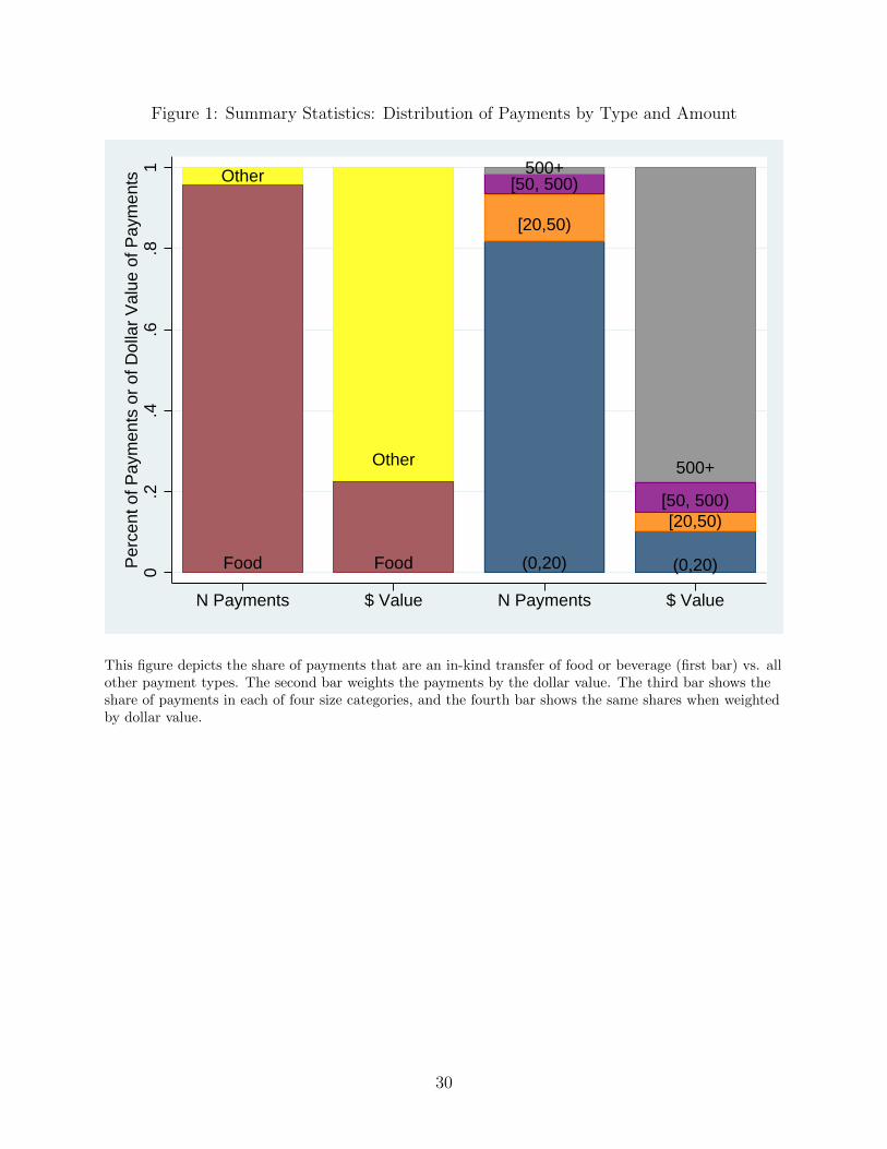
Figure 1: Summary Statistics: Distribution of Payments by Type and Amount

Food

Other

Food

Other

(0,20)

[20,50)

[50, 500)500+

(0,20)

[20,50)[50, 500)

500+

0.2

.4.6

.81

Per

cent

of P

aym

ents

or

of D

olla

r V

alue

of P

aym

ents

N Payments $ Value N Payments $ Value

This figure depicts the share of payments that are an in-kind transfer of food or beverage (first bar) vs. allother payment types. The second bar weights the payments by the dollar value. The third bar shows theshare of payments in each of four size categories, and the fourth bar shows the same shares when weightedby dollar value.

30

Table 1: Summary Statistics

Drug Indication% of Part DExpenditure

% ofExpenditureAffected byPayments

% ofPrescribingPhysiciansEver Paid

% ofPrescribingPhysiciansFirst Paid in14 or 15

All Drugs In Analytic Dataset 63 21 22 14Lantus Diabetes 3.3 24 16 9Harvoni Hep C 2.3 18 23 23Crestor High Cholesterol 2.3 23 18 9Advair Asthma/COPD 2.2 10 10 10Spiriva Asthma/COPD 1.9 26 21 11Abilify Mental Illness 1.9 28 24 8Januvia Diabetes 1.6 19 21 15Sovaldi Hep C 1.3 21 21 9Lyrica Nerve Pain 1.3 25 18 9Novolog Diabetes 1.2 27 27 17Levemir Diabetes 1.2 37 37 21Humira Immune Conds 1.1 45 66 27Namenda Dementia 1.1 2 1 0Enbrel Immune Conds 1.1 39 50 19Xarelto Blood Clots 1 44 45 24Zetia High Cholesterol 1 16 18 13Gleevec Cancer .9 6 13 5Symbicort Asthma/COPD .9 30 28 15Oxycontin Pain .8 23 21 12Humalog Diabetes .8 26 29 15

This table describes the prevalence of payments in Part D overall and for the twenty drugs with the largest totalexpenditure over the sample period. The third column describes the share of Part D expenditure. The next columndescribes the share of expenditure where the physician has received a payment for the drug at the time of prescribing.The next column describes the share of those who ever prescribe the drug who ever receive a payment for the drug.Finally, we report the share of prescribing physicians who are first paid in 2014 or 2015, since these physicians identifyour estimates given fixed effects.

31

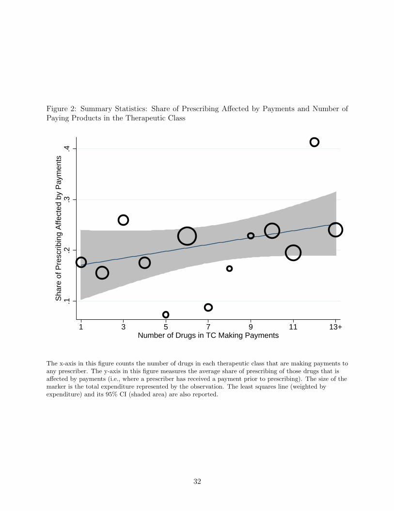
Figure 2: Summary Statistics: Share of Prescribing Affected by Payments and Number ofPaying Products in the Therapeutic Class

.1.2

.3.4

Sha

re o

f Pre

scrib

ing

Affe

cted

by

Pay

men

ts

1 3 5 7 9 11 13+Number of Drugs in TC Making Payments

The x-axis in this figure counts the number of drugs in each therapeutic class that are making payments toany prescriber. The y-axis in this figure measures the average share of prescribing of those drugs that isaffected by payments (i.e., where a prescriber has received a payment prior to prescribing). The size of themarker is the total expenditure represented by the observation. The least squares line (weighted byexpenditure) and its 95% CI (shaded area) are also reported.

32

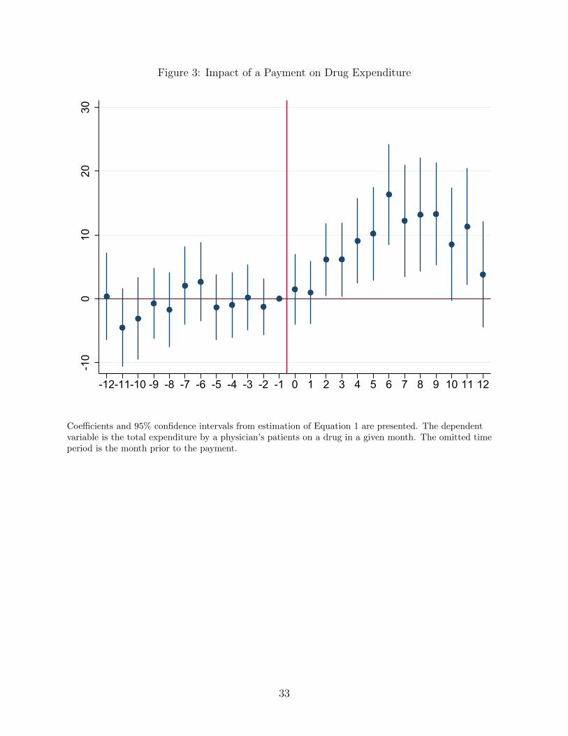
Figure 3: Impact of a Payment on Drug Expenditure-1

00

1020

30

-12-11-10 -9 -8 -7 -6 -5 -4 -3 -2 -1 0 1 2 3 4 5 6 7 8 9 10 11 12

Coefficients and 95% confidence intervals from estimation of Equation 1 are presented. The dependentvariable is the total expenditure by a physician’s patients on a drug in a given month. The omitted timeperiod is the month prior to the payment.

33

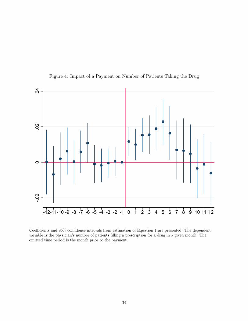
Figure 4: Impact of a Payment on Number of Patients Taking the Drug

-.02

0.0

2.0

4

-12-11-10 -9 -8 -7 -6 -5 -4 -3 -2 -1 0 1 2 3 4 5 6 7 8 9 10 11 12

Coefficients and 95% confidence intervals from estimation of Equation 1 are presented. The dependentvariable is the physician’s number of patients filling a prescription for a drug in a given month. Theomitted time period is the month prior to the payment.

34

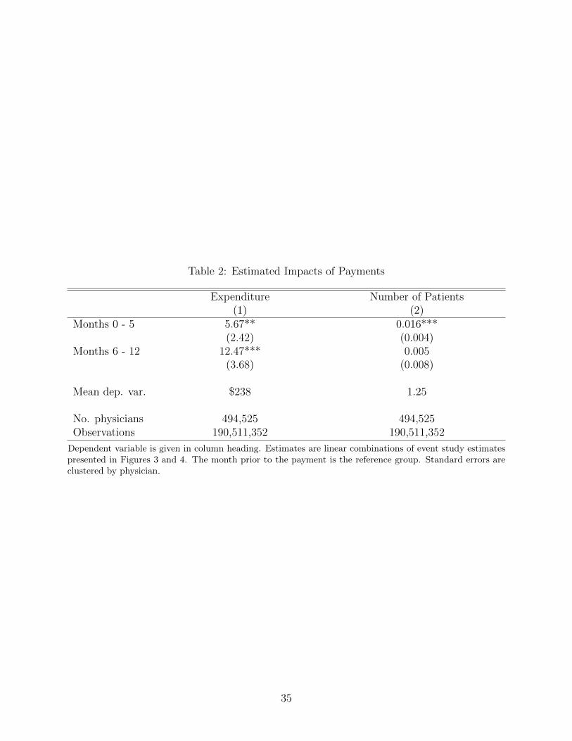
Table 2: Estimated Impacts of Payments

Expenditure Number of Patients(1) (2)

Months 0 - 5 5.67** 0.016***(2.42) (0.004)

Months 6 - 12 12.47*** 0.005(3.68) (0.008)

Mean dep. var. $238 1.25

No. physicians 494,525 494,525Observations 190,511,352 190,511,352

Dependent variable is given in column heading. Estimates are linear combinations of event study estimatespresented in Figures 3 and 4. The month prior to the payment is the reference group. Standard errors areclustered by physician.

35

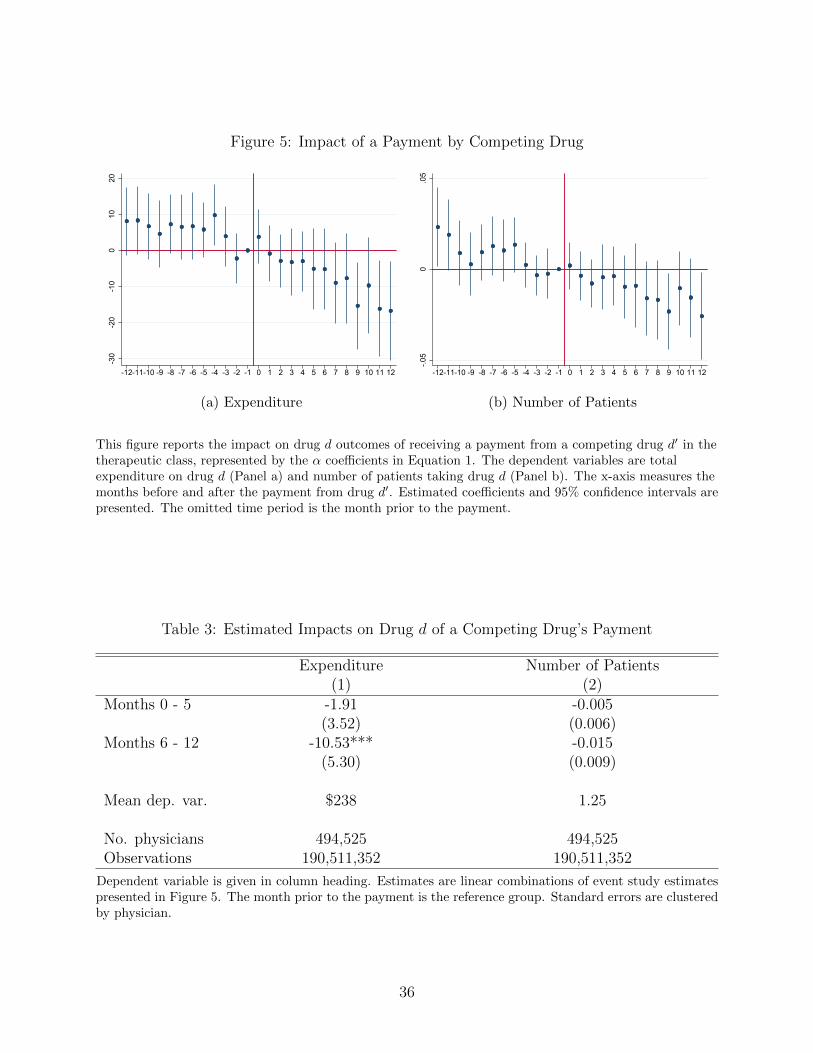
Figure 5: Impact of a Payment by Competing Drug

-30

-20

-10

010

20

-12-11-10 -9 -8 -7 -6 -5 -4 -3 -2 -1 0 1 2 3 4 5 6 7 8 9 10 11 12

(a) Expenditure

-.05

0.0

5

-12-11-10 -9 -8 -7 -6 -5 -4 -3 -2 -1 0 1 2 3 4 5 6 7 8 9 10 11 12

(b) Number of Patients

This figure reports the impact on drug d outcomes of receiving a payment from a competing drug d′ in thetherapeutic class, represented by the α coefficients in Equation 1. The dependent variables are totalexpenditure on drug d (Panel a) and number of patients taking drug d (Panel b). The x-axis measures themonths before and after the payment from drug d′. Estimated coefficients and 95% confidence intervals arepresented. The omitted time period is the month prior to the payment.

Table 3: Estimated Impacts on Drug d of a Competing Drug’s Payment

Expenditure Number of Patients(1) (2)

Months 0 - 5 -1.91 -0.005(3.52) (0.006)

Months 6 - 12 -10.53*** -0.015(5.30) (0.009)

Mean dep. var. $238 1.25

No. physicians 494,525 494,525Observations 190,511,352 190,511,352

Dependent variable is given in column heading. Estimates are linear combinations of event study estimatespresented in Figure 5. The month prior to the payment is the reference group. Standard errors are clusteredby physician.

36

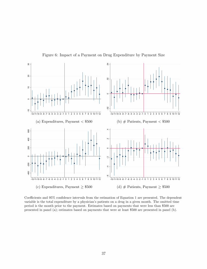
Figure 6: Impact of a Payment on Drug Expenditure by Payment Size

-10

010

2030

-12-11-10 -9 -8 -7 -6 -5 -4 -3 -2 -1 0 1 2 3 4 5 6 7 8 9 10 11 12

(a) Expenditures, Payment < $500

-.02

0.0

2.0

4

-12-11-10 -9 -8 -7 -6 -5 -4 -3 -2 -1 0 1 2 3 4 5 6 7 8 9 10 11 12

(b) # Patients, Payment < $500

-400

-200

020

040

060

0

-12-11-10 -9 -8 -7 -6 -5 -4 -3 -2 -1 0 1 2 3 4 5 6 7 8 9 10 11 12

(c) Expenditures, Payment ≥ $500

-.6-.4

-.20

.2.4

-12-11-10 -9 -8 -7 -6 -5 -4 -3 -2 -1 0 1 2 3 4 5 6 7 8 9 10 11 12

(d) # Patients, Payment ≥ $500

Coefficients and 95% confidence intervals from the estimation of Equation 1 are presented. The dependentvariable is the total expenditure by a physician’s patients on a drug in a given month. The omitted timeperiod is the month prior to the payment. Estimates based on payments that were less than $500 arepresented in panel (a); estimates based on payments that were at least $500 are presented in panel (b).

37

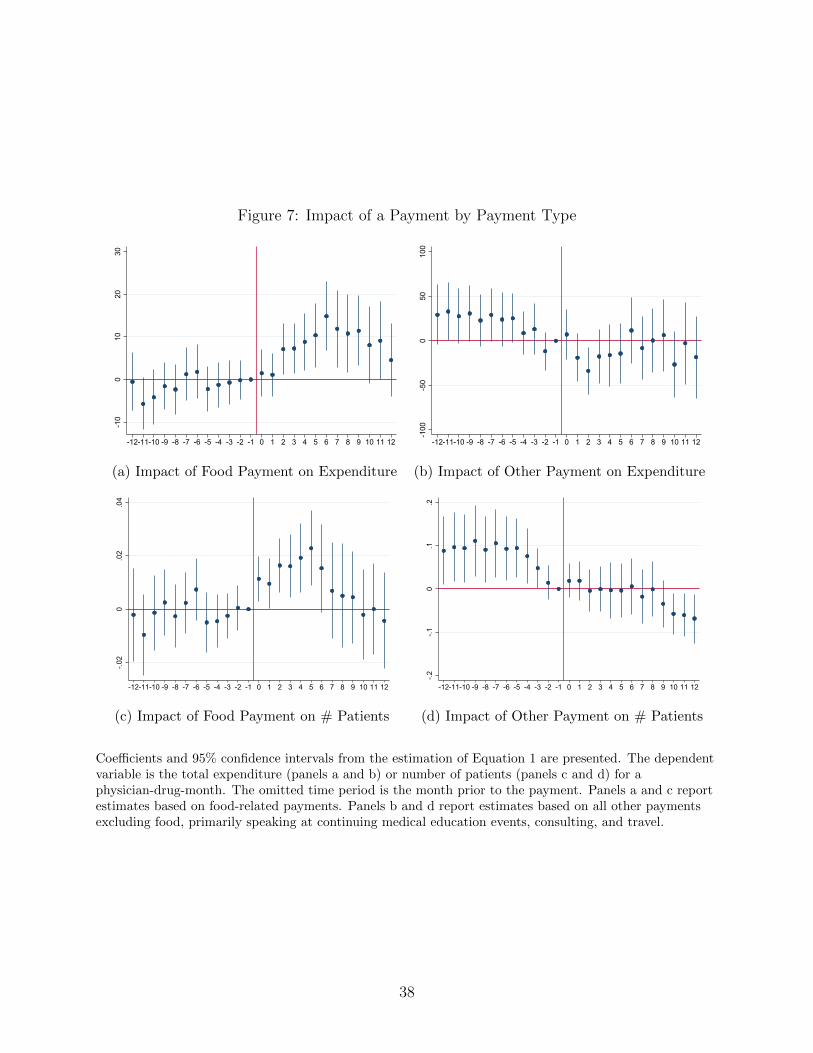
Figure 7: Impact of a Payment by Payment Type

-10

010

2030

-12-11-10 -9 -8 -7 -6 -5 -4 -3 -2 -1 0 1 2 3 4 5 6 7 8 9 10 11 12

(a) Impact of Food Payment on Expenditure

-100

-50

050

100

-12-11-10 -9 -8 -7 -6 -5 -4 -3 -2 -1 0 1 2 3 4 5 6 7 8 9 10 11 12

(b) Impact of Other Payment on Expenditure

-.02

0.0

2.0

4

-12-11-10 -9 -8 -7 -6 -5 -4 -3 -2 -1 0 1 2 3 4 5 6 7 8 9 10 11 12

(c) Impact of Food Payment on # Patients

-.2-.1

0.1

.2

-12-11-10 -9 -8 -7 -6 -5 -4 -3 -2 -1 0 1 2 3 4 5 6 7 8 9 10 11 12

(d) Impact of Other Payment on # Patients

Coefficients and 95% confidence intervals from the estimation of Equation 1 are presented. The dependentvariable is the total expenditure (panels a and b) or number of patients (panels c and d) for aphysician-drug-month. The omitted time period is the month prior to the payment. Panels a and c reportestimates based on food-related payments. Panels b and d report estimates based on all other paymentsexcluding food, primarily speaking at continuing medical education events, consulting, and travel.

38

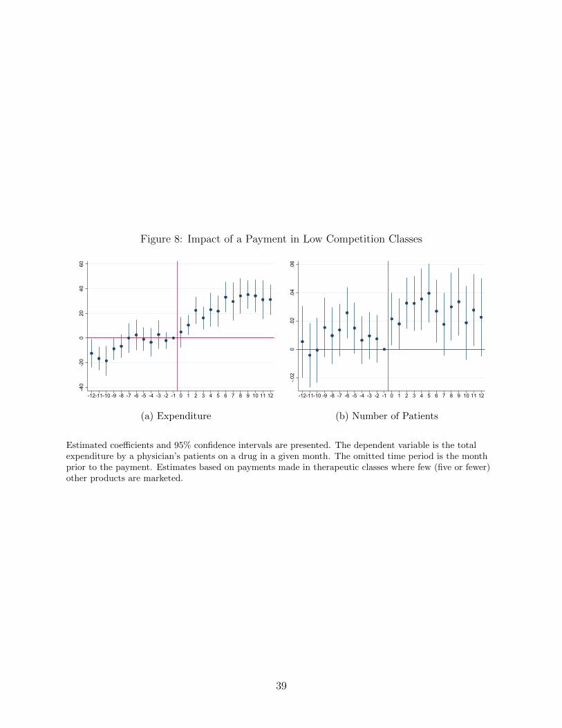
Figure 8: Impact of a Payment in Low Competition Classes

-40

-20

020

4060

-12-11-10 -9 -8 -7 -6 -5 -4 -3 -2 -1 0 1 2 3 4 5 6 7 8 9 10 11 12

(a) Expenditure

-.02

0.0

2.0

4.0

6

-12-11-10 -9 -8 -7 -6 -5 -4 -3 -2 -1 0 1 2 3 4 5 6 7 8 9 10 11 12

(b) Number of Patients

Estimated coefficients and 95% confidence intervals are presented. The dependent variable is the totalexpenditure by a physician’s patients on a drug in a given month. The omitted time period is the monthprior to the payment. Estimates based on payments made in therapeutic classes where few (five or fewer)other products are marketed.

39

Table 4: Heterogeneity in Estimated Impacts of Payments

Expenditure Number ofPatients

(1) (2)Panel A: Payment < $500Months 0 - 5 5.88** 0.016**

(2.39) (0.004)Months 6 - 12 11.18*** 0.005

(3.66) (0.008)Mean dep. var. $236 1.24

Panel B: Payment ≥ $500Months 0 - 5 -22.95 -0.03

(82.57) (0.06)Months 6 - 12 242.10*** -0.05

(91.60) (0.08)Mean dep. var. $233 1.31

Panel C: Food paymentMonths 0 - 5 6.03** 0.016***

(2.47) (0.005)Months 6 - 12 11.03*** 0.005

(3.78) (0.008)Mean dep. var. $238 1.24

Panel D: Other paymentMonths 0 - 5 -15.57 0.005

(12.54) (0.024)Months 6 - 12 -3.14 -0.028

(16.07) (0.024)Mean dep. var. $236 1.29

Panel E: Low competition class (5 or fewer paying drugs)Months 0 - 5 16.46*** 0.030***

(4.28) (0.008)Months 6 - 12 32.88*** 0.026***

(5.13) (0.011)Mean dep. var. $206.18 1.76

Dependent variable is given in column heading. Estimates are linear combinations of event study estimatespresented Figures 6, 7, and 8.

40

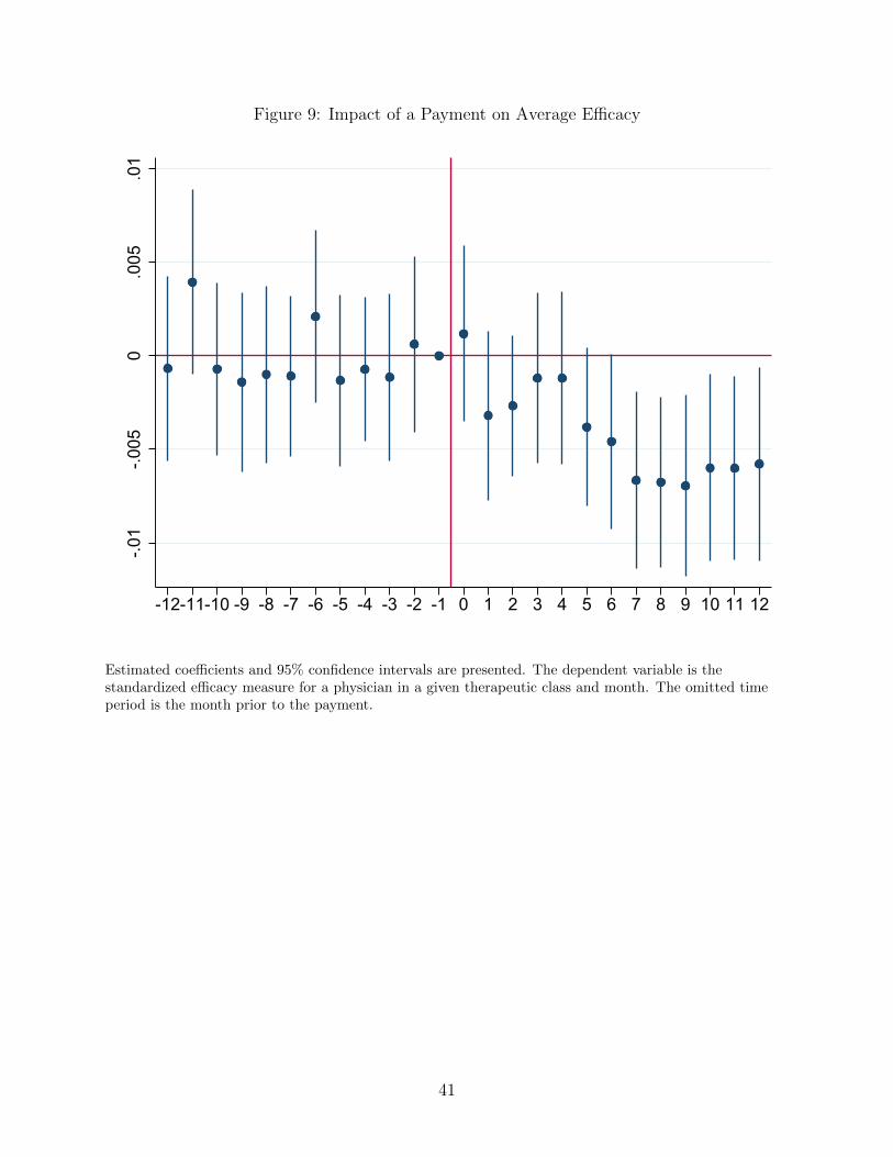
Figure 9: Impact of a Payment on Average Efficacy-.0

1-.0

050

.005

.01

-12-11-10 -9 -8 -7 -6 -5 -4 -3 -2 -1 0 1 2 3 4 5 6 7 8 9 10 11 12

Estimated coefficients and 95% confidence intervals are presented. The dependent variable is thestandardized efficacy measure for a physician in a given therapeutic class and month. The omitted timeperiod is the month prior to the payment.

41

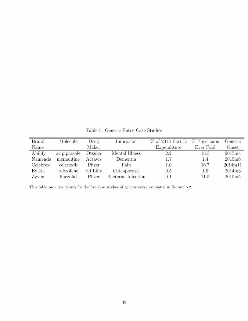
Table 5: Generic Entry Case Studies

Brand Molecule Drug Indication % of 2013 Part D % Physicians GenericName Maker Expenditure Ever Paid OnsetAbilify aripiprazole Otsuka Mental Illness 2.2 18.3 2015m4Namenda memantine Actavis Dementia 1.7 1.4 2015m6Celebrex celecoxib Pfizer Pain 1.0 16.7 2014m11Evista raloxifene Eli Lilly Osteoporosis 0.5 1.0 2014m3Zyvox linezolid Pfizer Bacterial Infection 0.1 11.5 2015m5

This table provides details for the five case studies of generic entry evaluated in Section 5.2.

42

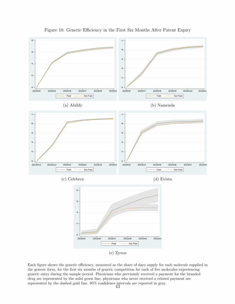
Figure 10: Generic Efficiency in the First Six Months After Patent Expiry0

.2.4

.6.8

2015m4 2015m5 2015m6 2015m7 2015m8 2015m9

Paid Not Paid

(a) Abilify

0.2

.4.6

.81

2015m6 2015m7 2015m8 2015m9 2015m10 2015m11

Paid Not Paid

(b) Namenda

0.2

.4.6

.81

2014m11 2014m12 2015m1 2015m2 2015m3 2015m4

Paid Not Paid

(c) Celebrex

0.2

.4.6

.81

2014m3 2014m4 2014m5 2014m6 2014m7 2014m8

Paid Not Paid

(d) Evista

0.2

.4.6

.8

2015m5 2015m6 2015m7 2015m8 2015m9 2015m10

Paid Not Paid

(e) Zyvox

Each figure shows the generic efficiency, measured as the share of days supply for each molecule supplied inthe generic form, for the first six months of generic competition for each of five molecules experiencinggeneric entry during the sample period. Physicians who previously received a payment for the brandeddrug are represented by the solid green line; physicians who never received a related payment arerepresented by the dashed gold line. 95% confidence intervals are reported in gray.

43

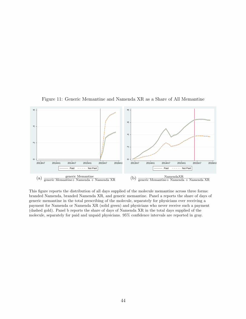
Figure 11: Generic Memantine and Namenda XR as a Share of All Memantine

0.2

.4.6

2013m7 2014m1 2014m7 2015m1 2015m7 2016m1

Paid Not Paid

(a) generic Memantinegeneric Memantine+ Namenda + Namenda XR

0.2

.4.6

.8

2013m7 2014m1 2014m7 2015m1 2015m7 2016m1

Paid Not Paid

(b) NamendaXRgeneric Memantine+ Namenda + Namenda XR

This figure reports the distribution of all days supplied of the molecule memantine across three forms:branded Namenda, branded Namenda XR, and generic memantine. Panel a reports the share of days ofgeneric memantine in the total prescribing of the molecule, separately for physicians ever receiving apayment for Namenda or Namenda XR (solid green) and physicians who never receive such a payment(dashed gold). Panel b reports the share of days of Namenda XR in the total days supplied of themolecule, separately for paid and unpaid physicians. 95% confidence intervals are reported in gray.

44

Appendices

A. Additional Figures and Tables

45

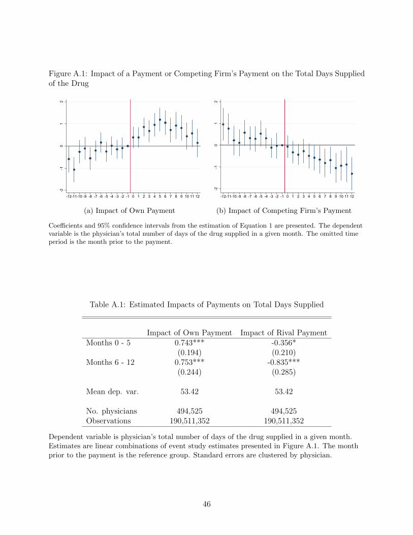
Figure A.1: Impact of a Payment or Competing Firm’s Payment on the Total Days Suppliedof the Drug

-2-1

01

2

-12-11-10 -9 -8 -7 -6 -5 -4 -3 -2 -1 0 1 2 3 4 5 6 7 8 9 10 11 12

(a) Impact of Own Payment-2

-10

12

-12-11-10 -9 -8 -7 -6 -5 -4 -3 -2 -1 0 1 2 3 4 5 6 7 8 9 10 11 12

(b) Impact of Competing Firm’s Payment

Coefficients and 95% confidence intervals from the estimation of Equation 1 are presented. The dependentvariable is the physician’s total number of days of the drug supplied in a given month. The omitted timeperiod is the month prior to the payment.

Table A.1: Estimated Impacts of Payments on Total Days Supplied

Impact of Own Payment Impact of Rival PaymentMonths 0 - 5 0.743*** -0.356*

(0.194) (0.210)Months 6 - 12 0.753*** -0.835***

(0.244) (0.285)

Mean dep. var. 53.42 53.42

No. physicians 494,525 494,525Observations 190,511,352 190,511,352

Dependent variable is physician’s total number of days of the drug supplied in a given month.Estimates are linear combinations of event study estimates presented in Figure A.1. The monthprior to the payment is the reference group. Standard errors are clustered by physician.

46

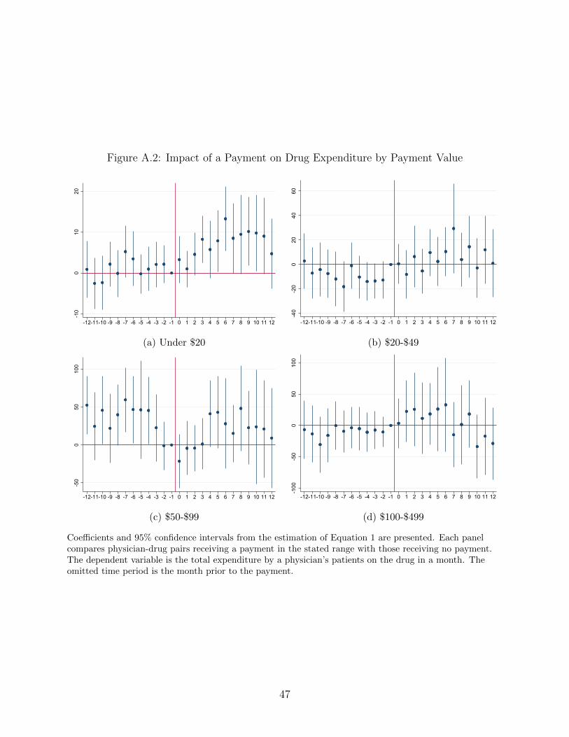
Figure A.2: Impact of a Payment on Drug Expenditure by Payment Value

-10

010

20

-12-11-10 -9 -8 -7 -6 -5 -4 -3 -2 -1 0 1 2 3 4 5 6 7 8 9 10 11 12

(a) Under $20

-40

-20

020

4060

-12-11-10 -9 -8 -7 -6 -5 -4 -3 -2 -1 0 1 2 3 4 5 6 7 8 9 10 11 12

(b) $20-$49

-50

050

100

-12-11-10 -9 -8 -7 -6 -5 -4 -3 -2 -1 0 1 2 3 4 5 6 7 8 9 10 11 12

(c) $50-$99

-100

-50

050

100

-12-11-10 -9 -8 -7 -6 -5 -4 -3 -2 -1 0 1 2 3 4 5 6 7 8 9 10 11 12

(d) $100-$499

Coefficients and 95% confidence intervals from the estimation of Equation 1 are presented. Each panelcompares physician-drug pairs receiving a payment in the stated range with those receiving no payment.The dependent variable is the total expenditure by a physician’s patients on the drug in a month. Theomitted time period is the month prior to the payment.

47

Figure A.3: Impact of a Payment on Expenditure and Patients: High Competition Classes

-60

-40

-20

020

40

-12-11-10 -9 -8 -7 -6 -5 -4 -3 -2 -1 0 1 2 3 4 5 6 7 8 9 10 11 12

(a) Expenditure

-.1-.0

50

.05

-12-11-10 -9 -8 -7 -6 -5 -4 -3 -2 -1 0 1 2 3 4 5 6 7 8 9 10 11 12

(b) Number of Patients

Estimated coefficients and 95% confidence intervals from the estimation of Equation 1 are presented arepresented for therapeutic classes with more than five drugs making payments over the sample period. Thedependent variable is the total expenditure of a physician’s patients on a drug (panel (a)) and the numberof patients on that drug (panel (b)) in a given month. The omitted time period is the month prior to thepayment.

48

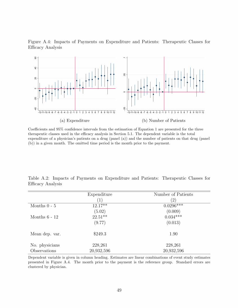
Figure A.4: Impacts of Payments on Expenditure and Patients: Therapeutic Classes forEfficacy Analysis

-40

-20

020

4060

-12-11-10 -9 -8 -7 -6 -5 -4 -3 -2 -1 0 1 2 3 4 5 6 7 8 9 10 11 12

(a) Expenditure-.0

50

.05

.1

-12-11-10 -9 -8 -7 -6 -5 -4 -3 -2 -1 0 1 2 3 4 5 6 7 8 9 10 11 12

(b) Number of Patients

Coefficients and 95% confidence intervals from the estimation of Equation 1 are presented for the threetherapeutic classes used in the efficacy analysis in Section 5.1. The dependent variable is the totalexpenditure of a physician’s patients on a drug (panel (a)) and the number of patients on that drug (panel(b)) in a given month. The omitted time period is the month prior to the payment.

Table A.2: Impacts of Payments on Expenditure and Patients: Therapeutic Classes forEfficacy Analysis

Expenditure Number of Patients(1) (2)

Months 0 - 5 12.17** 0.0296***(5.02) (0.009)

Months 6 - 12 22.51** 0.034***(9.77) (0.013)

Mean dep. var. $249.3 1.90

No. physicians 228,261 228,261Observations 20,932,596 20,932,596

Dependent variable is given in column heading. Estimates are linear combinations of event study estimatespresented in Figure A.4. The month prior to the payment is the reference group. Standard errors areclustered by physician.

49

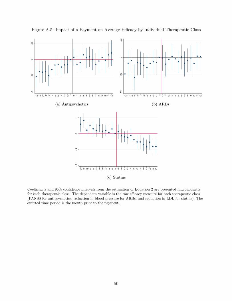
Figure A.5: Impact of a Payment on Average Efficacy by Individual Therapeutic Class-.1

-.05

0.0

5

-12-11-10 -9 -8 -7 -6 -5 -4 -3 -2 -1 0 1 2 3 4 5 6 7 8 9 10 11 12

(a) Antipsychotics

-.04

-.02

0.0

2

-12-11-10 -9 -8 -7 -6 -5 -4 -3 -2 -1 0 1 2 3 4 5 6 7 8 9 10 11 12

(b) ARBs

-.2-.1

0.1

-12-11-10 -9 -8 -7 -6 -5 -4 -3 -2 -1 0 1 2 3 4 5 6 7 8 9 10 11 12

(c) Statins

Coefficients and 95% confidence intervals from the estimation of Equation 2 are presented independentlyfor each therapeutic class. The dependent variable is the raw efficacy measure for each therapeutic class(PANSS for antipsychotics, reduction in blood pressure for ARBs, and reduction in LDL for statins). Theomitted time period is the month prior to the payment.

50

Table A.3: Impact of Payments on Drug Efficacy

Overall DrugEfficacy (StdDeviations)

Anti-psychotics(Improvement

in PANSS)

Statins (%Reduction in

LDL)

Angiotensin IIReceptorBlockers

(Reduction inSystolic BP)

Months 0 - 5 -0.0018 0.0022 -0.0172 -0.0026(0.0017) (0.0115) (0.0161) (0.0053)

Months 6 - 12 -0.0062*** 0.00027 -0.0663*** -0.0026(0.0019) (0.0149) (0.0176) (0.0.0058)

Mean dep. var. 13.92 37.44 9.22

No. physicians 496,834 210,249 421,989 316,760Observations 18,128,779 3,172,059 8,672,558 6,284,162

Dependent variable is given in column heading. Estimates are linear combinations of event study estimatespresented in Figure A.5. The month prior to the payment is the reference group. Standard errors areclustered by physician.

51

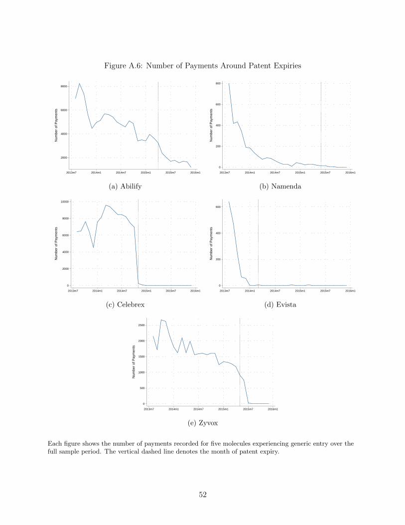
Figure A.6: Number of Payments Around Patent Expiries

2000

4000

6000

8000

Num

ber

of P

aym

ents

2013m7 2014m1 2014m7 2015m1 2015m7 2016m1

(a) Abilify

0

200

400

600

800

Num

ber

of P

aym

ents

2013m7 2014m1 2014m7 2015m1 2015m7 2016m1

(b) Namenda

0

2000

4000

6000

8000

10000

Num

ber

of P

aym

ents

2013m7 2014m1 2014m7 2015m1 2015m7 2016m1

(c) Celebrex

0

200

400

600

Num

ber

of P

aym

ents

2013m7 2014m1 2014m7 2015m1 2015m7 2016m1

(d) Evista

0

500

1000

1500

2000

2500

Num

ber

of P

aym

ents

2013m7 2014m1 2014m7 2015m1 2015m7 2016m1

(e) Zyvox

Each figure shows the number of payments recorded for five molecules experiencing generic entry over thefull sample period. The vertical dashed line denotes the month of patent expiry.

52