EE 6501 POWER SYSTEM ANALYSIS

Dr.P.USHA RANI

Professor, EEE Dept.

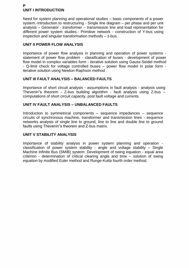
P UNIT I INTRODUCTION

Need for system planning and operational studies – basic components of a power system.-Introduction to restructuring - Single line diagram – per phase and per unit analysis – Generator - transformer – transmission line and load representation for different power system studies.- Primitive network - construction of Y-bus using inspection and singular transformation methods – z-bus.

UNIT II POWER FLOW ANALYSIS

Importance of power flow analysis in planning and operation of power systems - statement of power flow problem - classification of buses - development of power flow model in complex variables form - iterative solution using Gauss-Seidel method - Q-limit check for voltage controlled buses – power flow model in polar form - iterative solution using Newton-Raphson method .

UNIT III FAULT ANALYSIS – BALANCED FAULTS

Importance of short circuit analysis - assumptions in fault analysis - analysis using Thevenin‟s theorem - Z-bus building algorithm - fault analysis using Z-bus – computations of short circuit capacity, post fault voltage and currents.

UNIT IV FAULT ANALYSIS – UNBALANCED FAULTS

Introduction to symmetrical components – sequence impedances – sequence circuits of synchronous machine, transformer and transmission lines - sequence networks analysis of single line to ground, line to line and double line to ground faults using Thevenin‟s theorem and Z-bus matrix.

UNIT V STABILITY ANALYSIS

Importance of stability analysis in power system planning and operation - classification of power system stability - angle and voltage stability – Single Machine Infinite Bus (SMIB) system: Development of swing equation - equal area criterion - determination of critical clearing angle and time – solution of swing equation by modified Euler method and Runge-Kutta fourth order method.

TEXT BOOKS:

1. Nagrath I.J. and Kothari D.P., „Modern Power System Analysis‟, Tata McGraw-Hill, Fourth Edition, 2011. 2. John J. Grainger and W.D. Stevenson Jr., „Power System Analysis‟, Tata McGraw-Hill, Sixth reprint, 2010. 3. P. Venkatesh, B.V. Manikandan, S. Charles Raja, A. Srinivasan, „ Electrical Power Systems- Analysis, Security and Deregulation‟, PHI Learning Private Limited, New Delhi, 2012.

REFERENCES:

1. Hadi Saadat, „Power System Analysis‟, Tata McGraw Hill Education Pvt. Ltd., New Delhi,

21st

reprint, 2010.

2. Kundur P., „Power System Stability and Control, Tata McGraw Hill Education Pvt. Ltd., New Delhi, 10th reprint, 2010. 3. Pai M A, „Computer Techniques in Power System Analysis‟, Tata Mc Graw-Hill Publishing Company Ltd., New Delhi, Second Edition, 2007. 4. J. Duncan Glover, Mulukutla S. Sarma, Thomas J. Overbye, „ Power System Analysis & Design‟, Cengage Learning, Fifth Edition, 2012. 5. Olle. I. Elgerd, „Electric Energy Systems Theory – An Introduction‟, Tata McGraw Hill Publishing Company Limited, New Delhi, Second Edition, 2012. 6. C.A.Gross, “Power System Analysis,” Wiley India, 2011.

Chapter 1

POWER SYSTEM OVERVIEW

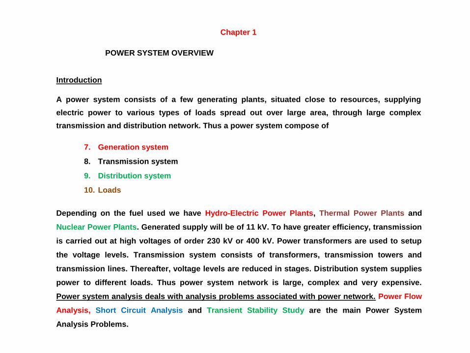
Introduction

A power system consists of a few generating plants, situated close to resources, supplying

electric power to various types of loads spread out over large area, through large complex

transmission and distribution network. Thus a power system compose of

7. Generation system

8. Transmission system

9. Distribution system

10. Loads

Depending on the fuel used we have Hydro-Electric Power Plants, Thermal Power Plants and

Nuclear Power Plants. Generated supply will be of 11 kV. To have greater efficiency, transmission

is carried out at high voltages of order 230 kV or 400 kV. Power transformers are used to setup

the voltage levels. Transmission system consists of transformers, transmission towers and

transmission lines. Thereafter, voltage levels are reduced in stages. Distribution system supplies

power to different loads. Thus power system network is large, complex and very expensive.

Power system analysis deals with analysis problems associated with power network. Power Flow

Analysis, Short Circuit Analysis and Transient Stability Study are the main Power System

Analysis Problems.

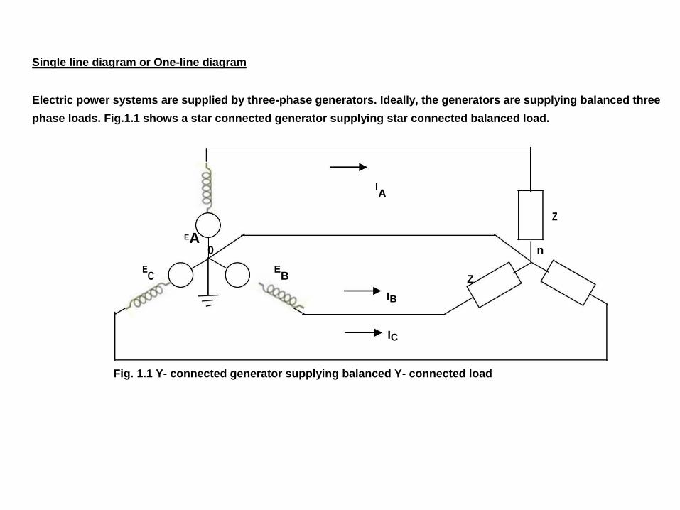
Single line diagram or One-line diagram

Electric power systems are supplied by three-phase generators. Ideally, the generators are supplying balanced three

phase loads. Fig.1.1 shows a star connected generator supplying star connected balanced load.

IA

Z

EA 0 n

EC

EB Z

IB

IC

Fig. 1.1 Y- connected generator supplying balanced Y- connected load

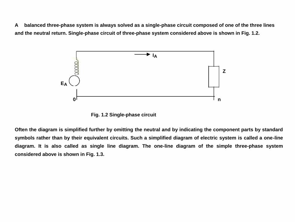
A balanced three-phase system is always solved as a single-phase circuit composed of one of the three lines

and the neutral return. Single-phase circuit of three-phase system considered above is shown in Fig. 1.2.

IA

Z

EA

0 n

Fig. 1.2 Single-phase circuit

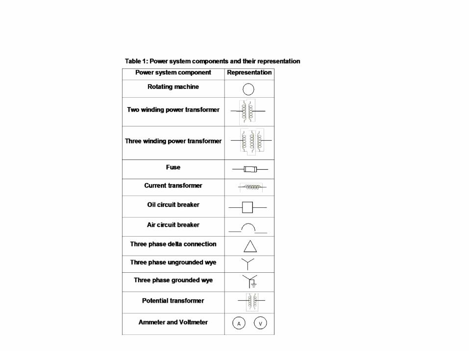
Often the diagram is simplified further by omitting the neutral and by indicating the component parts by standard

symbols rather than by their equivalent circuits. Such a simplified diagram of electric system is called a one-line

diagram. It is also called as single line diagram. The one-line diagram of the simple three-phase system

considered above is shown in Fig. 1.3.

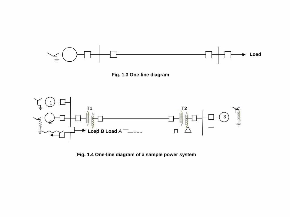
Load

Fig. 1.3 One-line diagram

1 T1 T2

3 2

Load B Load A

Fig. 1.4 One-line diagram of a sample power system

This system has two generators, one solidly grounded and the other grounded through a resistor, that are

connected to a bus and through a step-up transformer to a transmission line. Another generator, grounded

through a reactor, is connected to a bus and through a transformer to the other end of the transmission

line. A load is connected to each bus.

On the one-line diagram information about the loads, the ratings of the generators and transformers, and

reactances of different components of the circuit is often given.

Per phase analysis of symmetrical three phase systems

Per phase analysis of symmetrical three phase systems are illustrated through the following three

examples.

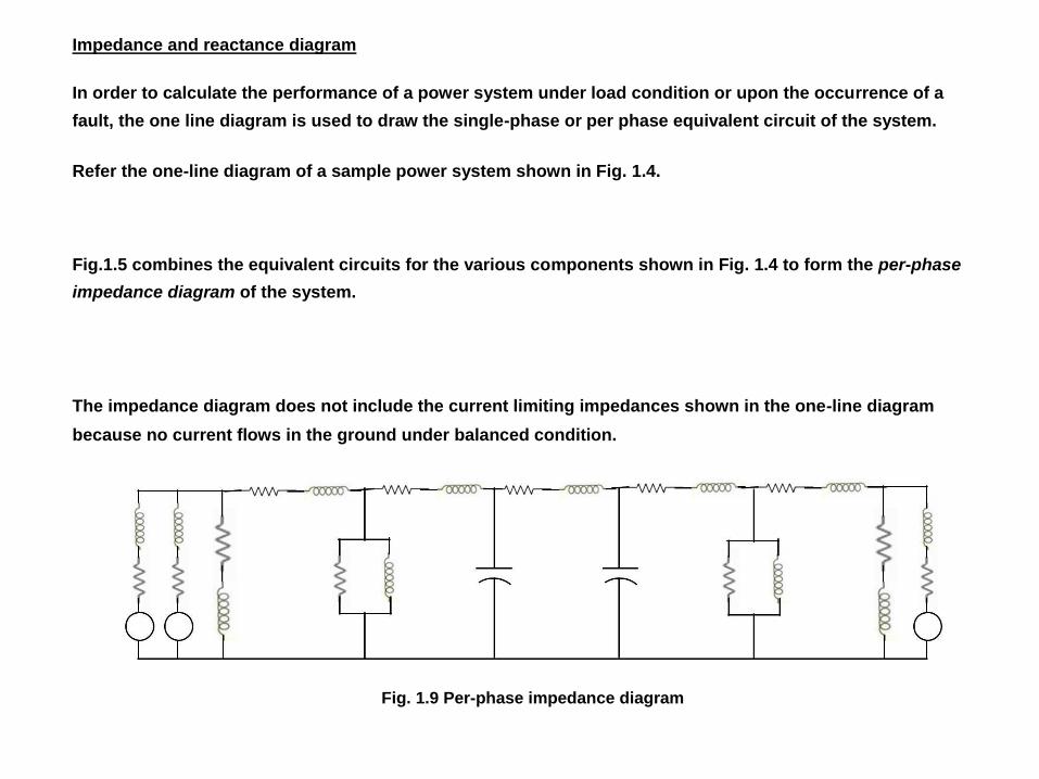
Impedance and reactance diagram

In order to calculate the performance of a power system under load condition or upon the occurrence of a

fault, the one line diagram is used to draw the single-phase or per phase equivalent circuit of the system.

Refer the one-line diagram of a sample power system shown in Fig. 1.4.

Fig.1.5 combines the equivalent circuits for the various components shown in Fig. 1.4 to form the per-phase

impedance diagram of the system.

The impedance diagram does not include the current limiting impedances shown in the one-line diagram

because no current flows in the ground under balanced condition.

Fig. 1.9 Per-phase impedance diagram

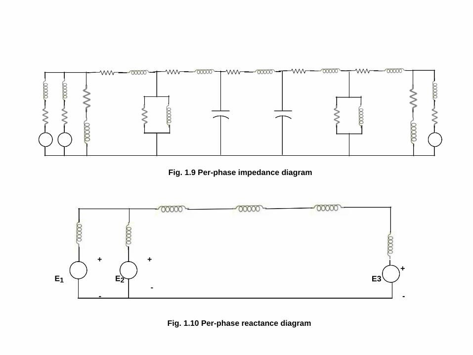
Fig. 1.9 Per-phase impedance diagram

+ + +

E1 E2 E3 - - -

Fig. 1.10 Per-phase reactance diagram

Per-unit quantities

Absolute values may not give the full significance of quantities. Consider the marks scored by a student in three

subjects as 10, 40 and 95. Many of you may be tempted to say that he is poor in subject 1, average in subject 2 and

good in subject 3. That is true only when the base for all the marks is 100. If the bases are 10, 50 and 100 for the

three subjects respectively then his marks in percentage are 100,80 and 95 and thus the conclusions are different.

Thus, there is a need to specify base quantity for meaningful interpretation.

Percentage = (actual value / base) x 100

Per-unit quantity = Percentage / 100 = actual value / base

This kind of explanation can be extended to all power system quantities.

In power system we shall deal with voltage, current, impedance and voltampere or power. When they are large

values, we may use kV, ampere, ohm and kVA or kW as their units. It is to be noted that out of the four quantities

voltage, current, impedance and voltampere if we specify two quantities, other two quantities can be calculated.

Generally, base voltampere in MVA and base voltage in kV are specified.

For a single-phase system, the following formulas relate the various quantities.

base VA base MVA x106

Base current, Abase voltage, V base voltage, kV x 1000

base MVA x 1000

=

(1.1)

base voltage, kV

base voltage, V base voltage, kV x1000

Base impedance , Ω (1.2) base current, A base current, A

Substituting eq. (1.1) in the above

(base voltage, kV)2

x 1000

Base impedance , Ω Thus

base MVA x1000

(base voltage, kV)2

Base impedance , Ω (1.3) base MVA

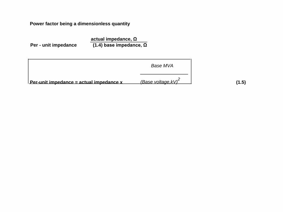
Power factor being a dimensionless quantity

actual impedance, Ω Per - unit impedance (1.4) base impedance, Ω

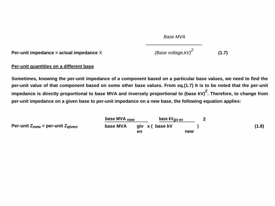
Base MVA

Per-unit impedance = actual impedance x (Base voltage,kV)2

(1.5)

For three phase system, when base voltage is specified it is line to line base voltage and the specified

MVA is three phase MVA. Now let us consider a three phase system. Let Base voltage, kV and Base

MVA be specified. Then single-

phase base voltage, kV = Base voltage, kV / 3 and single-phase base MVA=Base MVA / 3. Substituting

these in eq. (1.3)

[Base voltage, kV/ 3 ]2

(Basevoltage,kV)2

Base impedance , Ω (1.6) Base MVA / 3 Base MVA

It is to be noted that eq.(1.6) is much similar to eq.(1.3). Thus

actual impedance Per - unit impedance

baseimpedance

Base MVA

= actual impedance X (Base voltage,kV)2

(1.7)

(base voltage, kV)2

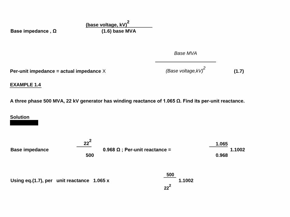
Base impedance , Ω (1.6) base MVA

Base MVA

Per-unit impedance = actual impedance X (Base voltage,kV)2

(1.7)

EXAMPLE 1.4

A three phase 500 MVA, 22 kV generator has winding reactance of 1.065 Ω. Find its per-unit reactance.

Solution

222 1.065

Base impedance 0.968 Ω ; Per-unit reactance = 1.1002 500 0.968

500

Using eq.(1.7), per unit reactance 1.065 x 1.1002

222

Base MVA

Per-unit impedance = actual impedance X (Base voltage,kV)2

(1.7)

Per-unit quantities on a different base

Sometimes, knowing the per-unit impedance of a component based on a particular base values, we need to find the

per-unit value of that component based on some other base values. From eq.(1.7) It is to be noted that the per-unit

impedance is directly proportional to base MVA and inversely proportional to (base kV)2. Therefore, to change from

per-unit impedance on a given base to per-unit impedance on a new base, the following equation applies:

base MVA new base kVgiv en 2

Per-unit Znew = per-unit Zgiven base MVA giv x ( base kV ) (1.8) en new

base MVA new base kVgiv en 2

Per-unit Znew = per-unit Zgiven x ( ) (1.8) base MVA giv base kV

en new

EXAMPLE 1.5

The reactance of a generator is given as 0.25 per-unit based on the generator’s of 18 kV, 500 MVA. Find its per-unit

reactance on a base of 20 kV, 100 MVA.

Solution

New per-unit reactance = 0.25 x 100

500 x ( 18

20 )2 = 0.0405

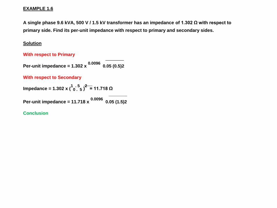
EXAMPLE 1.6

A single phase 9.6 kVA, 500 V / 1.5 kV transformer has an impedance of 1.302 Ω with respect to

primary side. Find its per-unit impedance with respect to primary and secondary sides.

Solution

With respect to Primary

Per-unit impedance = 1.302 x 0.0096

0.05 (0.5)2

With respect to Secondary

Impedance = 1.302 x (1

0..5

5 )2 = 11.718 Ω

Per-unit impedance = 11.718 x 0.0096

0.05 (1.5)2

Conclusion

Per-unit impedance of the transformer is same referred to primary as well as

secondary. Advantages of per-unit calculation

1. Manufacturers usually specify the impedance of a piece of apparatus in percent or per-unit on the

base of the name plate rating.

2. The per-unit impedances of machines of same type and widely different rating usually lie within

narrow range although the ohmic values differ much.

3. For a transformer, when impedance in ohm is specified, it must be clearly mentioned whether it is

with respect to primary or secondary. The per-unit impedance of the transformer, once expressed on

proper base, is the same referred to either side.

4. The way in which the three-phase transformers are connected does not affect the per-unit

impedances although the transformer connection does determine the relation between the voltage

bases on the two sides of the transformer.

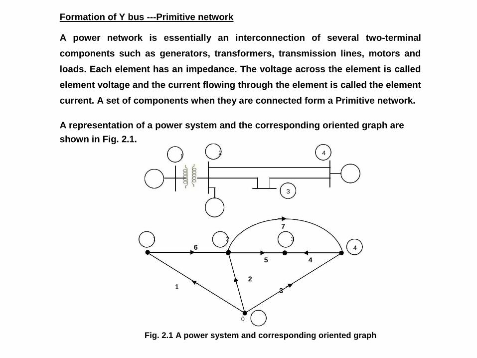
Formation of Y bus ---Primitive network

A power network is essentially an interconnection of several two-terminal

components such as generators, transformers, transmission lines, motors and

loads. Each element has an impedance. The voltage across the element is called

element voltage and the current flowing through the element is called the element

current. A set of components when they are connected form a Primitive network.

A representation of a power system and the corresponding oriented graph are

shown in Fig. 2.1.

1 2 4

3

7

1 2 3

6 4

5 4

2 1

3

0

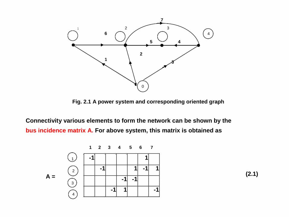
Fig. 2.1 A power system and corresponding oriented graph

7

1 2 3

6 4

5 4

2 1

3

0

Fig. 2.1 A power system and corresponding oriented graph

Connectivity various elements to form the network can be shown by the

bus incidence matrix A. For above system, this matrix is obtained as

1 2 3 4 5 6 7

1 -1 1

2 -1 1 -1 1 (2.1)

A =

-1 -1

3

4 -1 1 -1

Element voltages are referred as v1, v2, v3, v4, v5, v6 and v7. Element currents

are referred as i1, i2, i3, i4, i5, i6 and i7. In power system network, bus voltages

and bus currents are of more useful. For the above network, the bus voltages are

V1, V2, V3 and V4. The bus voltages are always measured with respect to the

ground bus. The bus currents are designated as I1, I2, I3, and I4. The element

voltages are related to bus voltages as:

7 v1 = - V1

1 2 3 v2 = - V2 6 4

5 4 v3 = - V4

2 v4 = V4 – V3 1

3

v5 = V2 - V3

v6 = V1 – V2 0

v7 = V2 – V4

Expressing the relation in matrix form

-1 V

1 v1

-1

v2

v -1 V2 v

3

=

-1 1

4

v

V3

1

-1

v5

1

-1

6 V4

v 7 1 -1

Thus v = AT V

bus

The element currents are related to bus currents as:

7

I2

6 I3

I4

I1

5 4

2 3 4 1

2

1

3

(2.2)

(2.3)

I1 = - i1 + i6

I2 = - i2 + i5 – i6 + i7

I3 = - i4 – i5

I4 = - i3 + i4 – i7

0

I1 = - i1 + i6

I2 = - i2 + i5 – i6 + i7

I3 = - i4 – i5

I4 = - i3 + i4 – i7

Expressing the relation in matrix form

I1 -1 1

-1 1 -1 1 2

I3 = -1 -1

-1 1 -1 4

Thus Ibus = A i

i1

i2

i3

i4

i5

i6

i7 (2.4)

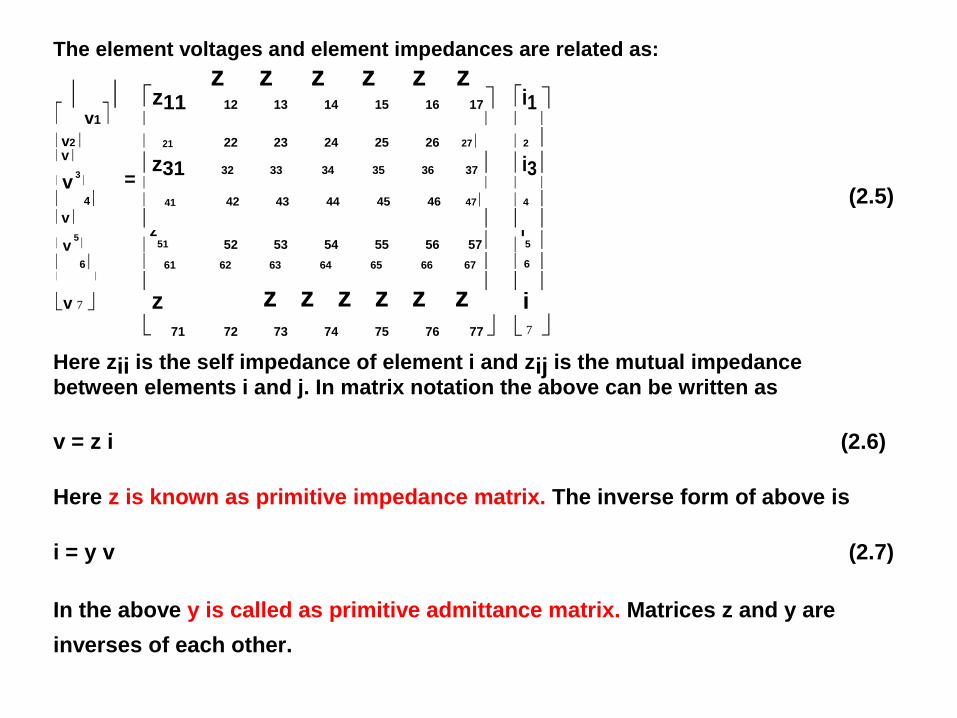
The element voltages and element impedances are related as:

z11

z z z z z z i1

12 13 14 15 16 17

v1

v2 21 22 23 24 25 26 27 2 v

z31

i3

v3

=

32 33 34 35 36 37

(2.5) 4 41 42 43 44 45 46 47 4 v

v5

z51 52 53 54 55 56 57

i5

6 61 62 63 64 65 66 67 6

z z z z z z

v 7 z

i

71 72 73 74 75 76 77 7

Here zii is the self impedance of element i and zij is the mutual impedance

between elements i and j. In matrix notation the above can be written as

v = z i (2.6)

Here z is known as primitive impedance matrix. The inverse form of above is

i = y v (2.7)

In the above y is called as primitive admittance matrix. Matrices z and y are

inverses of each other.

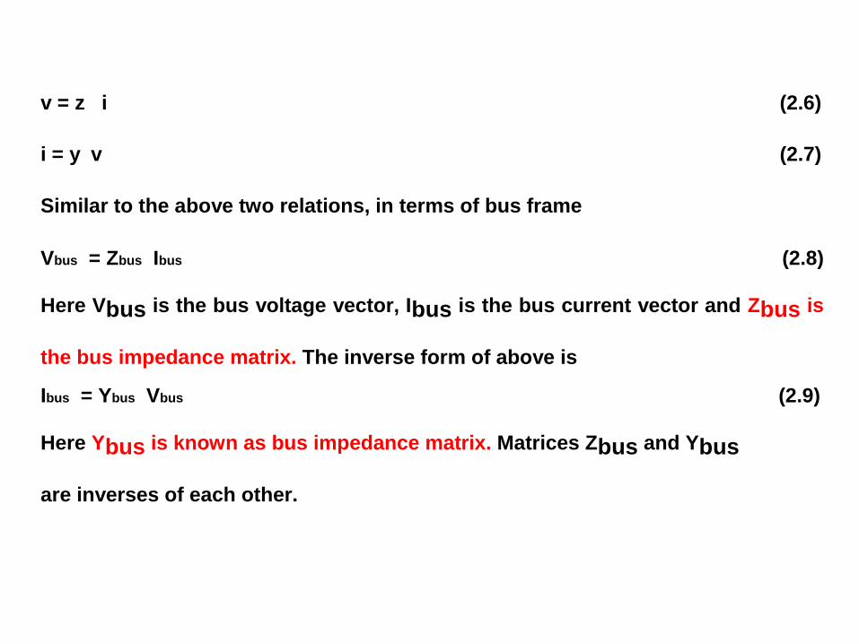
v = z i (2.6)

i = y v (2.7)

Similar to the above two relations, in terms of bus frame

Vbus = Zbus Ibus (2.8)

Here Vbus is the bus voltage vector, Ibus is the bus current vector and Zbus is

the bus impedance matrix. The inverse form of above is

Ibus = Ybus Vbus (2.9)

Here Ybus is known as bus impedance matrix. Matrices Zbus and Ybus

are inverses of each other.

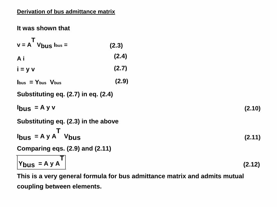
Derivation of bus admittance matrix It was shown that

v = AT

Vbus Ibus =

A i

i = y v Ibus = Ybus Vbus

Substituting eq. (2.7) in eq. (2.4)

Ibus = A y v Substituting eq. (2.3) in the above

Ibus = A y AT

Vbus Comparing eqs. (2.9) and (2.11)

(2.10) (2.11)

Ybus = A y AT

(2.12)

This is a very general formula for bus admittance matrix and admits mutual

coupling between elements.

(2.3)

(2.4)

(2.7)

(2.9)

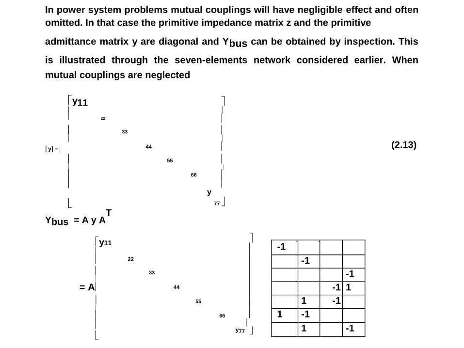
In power system problems mutual couplings will have negligible effect and often

omitted. In that case the primitive impedance matrix z and the primitive

admittance matrix y are diagonal and Ybus can be obtained by inspection. This

is illustrated through the seven-elements network considered earlier. When

mutual couplings are neglected

y11 22

y

Ybus = A y AT

y11

= A

33

44

55

66

22

33

44

55

y

77

66

y77

(2.13)

-1

-1

-1

-1 1

1 -1

1 -1

1 -1

-y11

-y22

= -1 1

-y33 -1 1 -1 1

-y44 y44

-1 -1

y55 -y55

-1 1

-1

y66 -y66

y77 -y77

1 2 3 4

1 y11 + y66 - y66 0 0

2 - y66 y22 + y55 + y66+y77 - y55 - y77

Ybus = 3 0 - y55 y44 + y55 - y44

4 0 - y77 - y44 y33 + y44 + y77

1 2 3 4

1 y11 + y66 - y66 0 0

2

- y66 y22 + y55 + y66+y77

- y55

- y77

Ybus = 3 0 - y55 y44 + y55 - y44

4 0

- y77

- y44 y33 + y44 + y77

7

1 2 3 6 4

5 4

2 1

3

0

The rules to form the elements of Ybus are:

The diagonal element Yii equals the sum of the admittances directly

connected to bus i.

The off-diagonal element Yij equals the negative of the admittance

connected between buses i and j. If there is no element between buses

i and j, then Yij equals to zero.

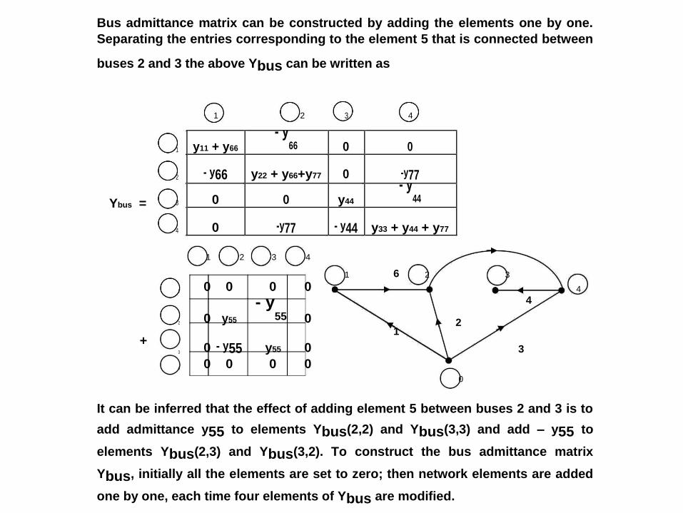
Bus admittance matrix can be constructed by adding the elements one by one.

Separating the entries corresponding to the element 5 that is connected between

buses 2 and 3 the above Ybus can be written as

Ybus =

+

1 2 3 4

1 y11 + y66

- y66 0 0

2 - y66 y22 + y66+y77 0 -y77

3 0 0 y44

- y44

4 0 -y77 - y44 y33 + y44 + y77

1 2 3 4

1 6 2 3

1 0 0 0 0 4

- y55

4

2 0 y55 0 2

1

0 - y55 y55 0

3 3

4 0 0 0 0

0

It can be inferred that the effect of adding element 5 between buses 2 and 3 is to

add admittance y55 to elements Ybus(2,2) and Ybus(3,3) and add – y55 to

elements Ybus(2,3) and Ybus(3,2). To construct the bus admittance matrix

Ybus, initially all the elements are set to zero; then network elements are added

one by one, each time four elements of Ybus are modified.

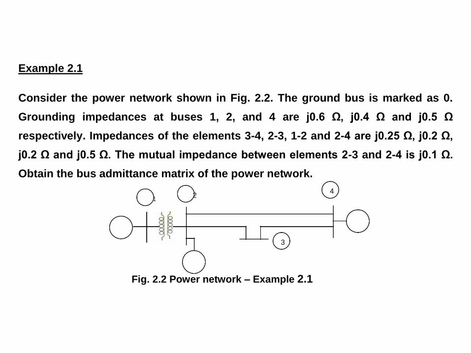
Example 2.1

Consider the power network shown in Fig. 2.2. The ground bus is marked as 0.

Grounding impedances at buses 1, 2, and 4 are j0.6 Ω, j0.4 Ω and j0.5 Ω

respectively. Impedances of the elements 3-4, 2-3, 1-2 and 2-4 are j0.25 Ω, j0.2 Ω,

j0.2 Ω and j0.5 Ω. The mutual impedance between elements 2-3 and 2-4 is j0.1 Ω.

Obtain the bus admittance matrix of the power network.

1 2

4

3

Fig. 2.2 Power network – Example 2.1

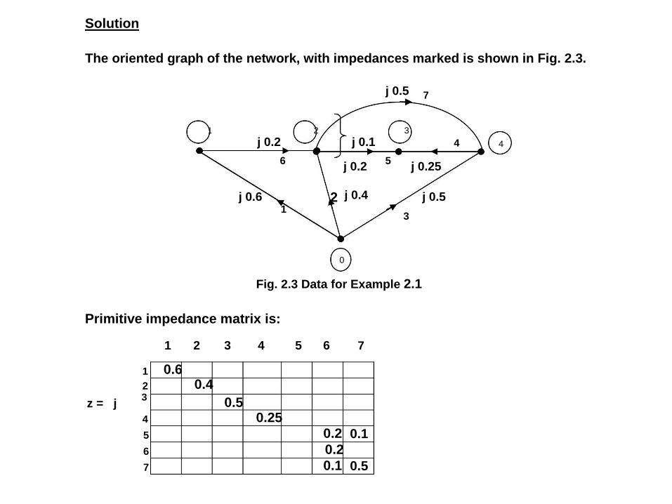
Solution

The oriented graph of the network, with impedances marked is shown in Fig. 2.3.

j 0.5 7

1 2 3

j 0.2 j 0.1 4 4

6 j 0.2

5 j 0.25

j 0.6 2 j 0.4 j 0.5 1

3

0

Fig. 2.3 Data for Example 2.1

Primitive impedance matrix is:

1 2 3 4 5 6 7

1 0.6

2 0.4

z = j 3

0.5

4 0.25

5 0.2 0.1

6 0.2

7 0.1 0.5

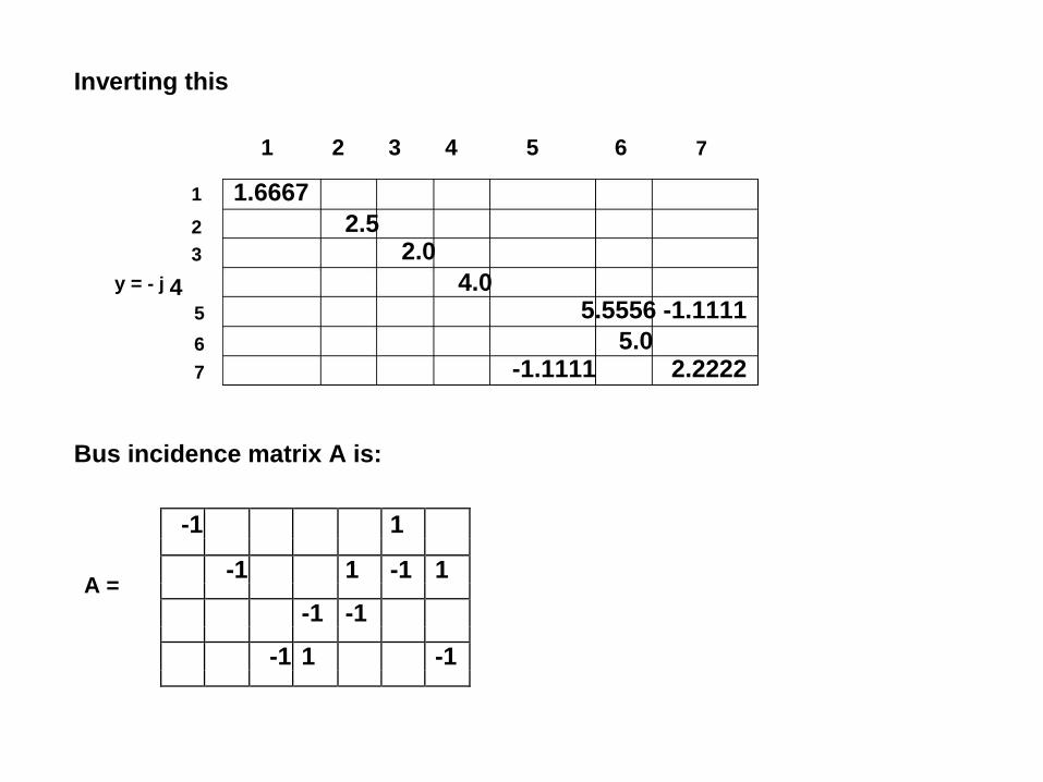
Inverting this

1 2 3 4 5 6 7

1 1.6667

2 2.5

3 2.0

y = - j 4 4.0

5 5.5556 -1.1111

6 5.0

7 -1.1111 2.2222

Bus incidence matrix A is:

-1 1

A = -1 1 -1 1

-1 -1

-1 1 -1

Bus admittance matrix Ybus = A y AT

1.6667 -1

2.5

-1

Ybus = - j A

2.0

-1 4.0

-1 1 5.5556 -1.1111

5.0 1 -1

-1.1111

2.2222

1 -1

1 -1

-1.6667

-1 1 - 2.5

- 2.0 -1 1 -1 1

Ybus = - j

- 4.0 4.0 -1 -1

4.4444 - 5.5556 1.1111

-1 1

-1

5.0 - 5.0

1.1111 1.1111 - 2.2222

1 2 3 4

1

2

Ybus = 3

4

- j6.6667 j5.0 0 0

j5.0 - j13.0556 j4.4444 j1.1111

0 j4.4444 - j9.5556 j5.1111

0 j1.1111 j5.1111 - j8.2222