RESEARCH ARTICLE10.1002/2016WR020086

Droughts in Amazonia: Spatiotemporal Variability,Teleconnections, and Seasonal PredictionsCarlos H. R. Lima1 and Amir AghaKouchak2

1Department of Civil and Environmental Engineering, University of Brasilia, Brasilia, DF, Brazil, 2Department of Civil andEnvironmental Engineering, University of California, Irvine, CA, USA

Abstract Most Amazonia drought studies have focused on rainfall deficits and their impact on river dis-charges, while the analysis of other important driver variables, such as temperature and soil moisture, hasattracted less attention. Here we try to better understand the spatiotemporal dynamics of Amazoniadroughts and associated climate teleconnections as characterized by the Palmer Drought Severity Index(PDSI), which integrates information from rainfall deficit, temperature anomalies, and soil moisture capacity.The results reveal that Amazonia droughts are most related to one dominant pattern across the entireregion, followed by two seesaw kind of patterns: north-south and east-west. The main two modes are corre-lated with sea surface temperature (SST) anomalies in the tropical Pacific and Atlantic oceans. The telecon-nections associated with global SST are then used to build a seasonal forecast model for PDSI overAmazonia based on predictors obtained from a sparse canonical correlation analysis approach. A uniquefeature of the presented drought prediction method is using only a few number of predictors to avoidexcessive noise in the predictor space. Cross-validated results show correlations between observed and pre-dicted spatial average PDSI up to 0.60 and 0.45 for lead times of 5 and 9 months, respectively. To the bestof our knowledge, this is the first study in the region that, based on cross-validation results, leads to appre-ciable forecast skills for lead times beyond 4 months. This is a step forward in better understanding thedynamics of Amazonia droughts and improving risk assessment and management, through improveddrought forecasting.

1. Introduction

The dynamics of the Amazonia ecosystem plays a significant role on the global biogeochemical cycles(McClain et al., 2001), wild fires (Chen et al., 2013), moisture transport to southeast South America (Dru-mond et al., 2008), regional and global climate (Nobre et al., 1991; Spracklen & Garcia-Carreras, 2015), andon local population (Marengo & Espinoza, 2016). In particular, extreme droughts in the Amazonia seem tohave become more frequent in the last years (e.g., Marengo & Espinoza, 2016) and studies have showntheir significant impacts on the regional ecosystem and biogeochemical cycles (Cochrane, 2003; Feld-pausch et al., 2016; Laurance & Williamson, 2001; Maeda et al., 2015; Phillips et al., 2009), wild fires (Arag~aoet al., 2007), and on the local hydrological cycle (Lopes et al., 2016; Marengo et al., 2008a). Eventually,these changes in Amazonia propagate to distant regions because of large-scale atmospheric circulationdynamics. For instance, during austral summer, water vapor from Amazonia is transported to southeastSouth America (Arraut et al., 2012; Drumond et al., 2008; Silva & Ambrizzi, 2009). Changes in evapotranspi-ration in response to a drought will certainly change the water vapor transport—although the exactmechanisms and magnitude are still unknown—and affect water supply and hydropower generation insoutheast South America.

Motivated by these ecosystem and socioeconomic impacts, a substantial number of studies (e.g., Arrautet al., 2012; Espinoza et al., 2011; Marengo, 1992; Marengo & Espinoza, 2016; Marengo et al., 2008b, 2011;Ropelewski & Halpert, 1987; Yoon & Zeng, 2010; and references therein) have tried to better understand thedynamics of droughts in Amazonia. The main cause of droughts in Amazonia has been attributed to the ElNi~no-Southern Oscillation (ENSO) and to a minor extent to the sea surface temperature (SST) variability inthe Tropical North Atlantic. Warm SST anomalies in the eastern Tropical Pacific shift the descending branchof the Walker circulation over Amazonia and inhibit precipitation during the austral summer rainfall season.A warmer tropical north Atlantic will displace north the Inter-Tropical Convergence Zone from its

Key Points:� Spatiotemporal dynamics and

teleconnections associated withAmazonia droughts are investigatedbased on the PDSI indices� A drought forecast model for

Amazonia is developed and testedbased on the global SST field andsparse canonical correlation analysis� This is the first study in the region

that, based on cross-validation, leadsto appreciable forecast skills for leadtimes beyond 4 months

Supporting Information:� Supporting Information S1

Correspondence to:C. H. R. Lima,chrlima@unb.br

Citation:Lima, C. H. R., & AghaKouchak, A.(2017). Droughts in Amazonia:Spatiotemporal variability,teleconnections, and seasonalpredictions. Water Resources Research,53, 10,824–10,840. https://doi.org/10.1002/2016WR020086

Received 7 NOV 2016

Accepted 8 DEC 2017

Accepted article online 13 DEC 2017

Published online 29 DEC 2017

Corrected 30 JAN 2018

This article was corrected on 30 JAN

2018. See the end of the full text for

details.

VC 2017. American Geophysical Union.

All Rights Reserved.

LIME AND AGHAKOUCHAK DROUGHTS IN AMAZONIA 10,824

Water Resources Research

PUBLICATIONS

climatological position and therefore the ascending branch of the Hadley cell and reduce convection andprecipitation over Amazonia.

Most studies on Amazonia droughts have primarily focused on rainfall variability (Arag~ao et al., 2007; Zouet al., 2016) and its teleconnections (Fernandes et al., 2015; Marengo, 1992; Yoon & Zeng, 2010), and theassociated impacts on river flows across Amazonia (Espinoza et al., 2011; Lopes et al., 2016; Marengo et al.,2008b). We perceive that little is known about the compounding effects of rainfall and temperature overAmazonia, and how these two variables exacerbate drought impacts, particularly on the vegetation and nat-ural ecosystem. On the other hand, the state of soil moisture could indicate water deficit caused by not onlyprecipitation deficit but also excess evapotranspiration. Previous studies show that univariate drought riskassessment approaches based solely on rainfall can severely underestimate the underlying risk of extremedroughts (AghaKouchak et al., 2014; Shukla et al., 2015) and their impacts (Williams et al., 2013), and a multi-variate approach can provide a more realistic assessment. In this sense, the use of drought indices that inte-grate different hydroclimate variables (e.g., rainfall, temperature, soil moisture, etc.), such as the PalmerDrought Severity Index (Palmer, 1965) and the Multivariate Standardized Drought Index (Hao & AghaKou-chak, 2014) might reveal atmospheric and land conditions associated with water stress that are more suit-able to investigate droughts and their impacts. In the case of Amazonia droughts, we perceive that just few,limited-scope studies (e.g., Dai, 2011; Dai et al., 2004; Jim�enez-Mu~noz et al., 2016; Joetzjer et al., 2013) havelooked at drought indices and such field deserves further investigation, particularly in terms of understand-ing the variability of such indices, teleconnections associated, and predictive models for long-termforecasts.

Understanding and prediction of droughts across the world have been the subject of much research (e.g.,Cook et al., 2010; Funk et al., 2014; Hoerling et al., 2012; Kwon et al., 2016; Lyon et al., 2012; Rajagopalanet al., 2000; Schubert et al., 2007; Seager et al., 2015; Thober et al., 2015) and some drought monitor systems(e.g., the U.S. Drought Monitor, http://droughtmonitor.unl.edu/Home.aspx and the Latin American DroughtMonitor, http://stream.princeton.edu/LAFDM/WEBPAGE/interface.php?locale5en) plan or have already inte-grated seasonal drought forecasts. Here, we aim to advance the current Brazilian initiatives for droughtmonitoring (e.g., the INPE drought monitor, http://clima1.cptec.inpe.br/spi/pt) through a multivariateapproach for drought analysis and prediction across Amazonia. This work is then carried out to betterunderstand the spatiotemporal dynamics of droughts in Amazonia as informed by the widely used PalmerDrought Severity Index, PDSI (Alley, 1984; Dai et al., 2004; Palmer, 1965). Recently, it has been successfullyused to study Amazonia droughts (Jim�enez-Mu~noz et al., 2016), mainly to investigate the relationshipbetween the largest El Ni~no events in the last years (1982–1983, 1997–1998, and 2015–2016) and thedrought severity and spatial distribution across Amazonia. We study sea surface temperature (SST) telecon-nections and develop and test a long-term (up to 9 months lead time) forecast model for PDSI over Amazo-nia. We employ a linear model and exogenous predictors derived from the SST teleconnections and basedon a sparse canonical correlation analysis (Zou et al., 2006), which essentially seeks to maximize the correla-tion of two projected sub spaces of two fields (Hotelling, 1936), while trying to minimize the noise effect inthe projected variables by shrinking the associated canonical coefficients. After this introduction, this workis organized as follows. In the next section, we present the data set. In section 3, we analyze the spatiotem-poral patterns of PDSI across Amazonia, and in section 4 we investigate the associated teleconnections withthe global SST field. In section 5, we introduce the predictive model for PDSI and evaluate its forecast skillfor different lead times based on a cross-validation procedure. Finally, in section 6, we offer a summary ofthe results found in the paper and present some conclusions.

2. Climate Data Set

2.1. PDSI Drought IndicesWe use a variant of the Palmer Drought Severity Index (PDSI), originally proposed by Palmer (1965) to inves-tigate drought conditions. It is one of the most widely used indices for drought characterization, although ithas some limitations (Alley, 1984; Hayes et al., 1999; Heim, 2002; Keyantash & Dracup, 2002; Mishra & Singh,2010), particularly its underestimation of runoff, delayed response in detecting some droughts, and moresuitability for agricultural droughts. PDSI is obtained by relating temperature, rainfall, and soil-water holdingcapacity to estimate a local water balance and define local moisture stress conditions. We refer the reader

Water Resources Research 10.1002/2016WR020086

LIME AND AGHAKOUCHAK DROUGHTS IN AMAZONIA 10,825

to Palmer (1965) and Wells et al. (2004) for the mathematical details on how to estimate the PDSI. Here weuse the self-calibrated PDSI (Wells et al., 2004), which intends to replace empirical constants as used in thetraditional PDSI calibration by dynamically estimated characteristics of the given location, which in turnmakes the PDSI more comparable across space (Wells et al., 2004). The self-calibrated PDSI is usuallyreferred in the literature as scPDSI. In this paper, for simplicity, we refer to it as PDSI. PDSI information is esti-mated by Dai et al. (2004) and consist of gridded, monthly values over Amazonia as defined in Figure 1 forthe period 1980–2013. The data are available at http://www.esrl.noaa.gov/psd/.

2.2. Global Sea Surface TemperatureHere, we use monthly SST data from the ERA Interim global sea surface temperature archive for the period1980–2013. The data set is interpolated onto a 2.58 3 2.58 grid and is available at http://apps.ecmwf.int/datasets/data/interim-full-moda/levtype5sfc/.

2.3. Rainfall and TemperatureMonthly gridded (0.258 3 0.258) temperature and rainfall data for the period 1980–2013 are provided byXavier et al. (2016). These data consist of interpolated daily rainfall and temperature observations from3,625 rainfall gauges and 735 weather stations across Brazil available from different institutions (INMET,ANA, and DAEE). The interpolation schemes and validation procedures are described in Xavier et al. (2016).Note that these data are delimited by the Brazilian Amazonia boundary as defined by the states of Amazo-nas, Roraima, Par�a, Rondonia, Mato Grosso, and Acre and shown in Figure 1. For each grid point, monthlyanomalies of rainfall and temperature are obtained by removing from the observed value the long-termmonthly mean for that grid point based on the 1980–2013 period. The data are also spatially constrained tothe PDSI grid domain as shown in Figure 1.

−80 −70 −60 −50 −40 −30

−30

−20

−10

010

−80 −70 −60 −50 −40 −30

−30

−20

−10

010

FORLANDURBSNOW

AM

AC

PA

MTRO

RR

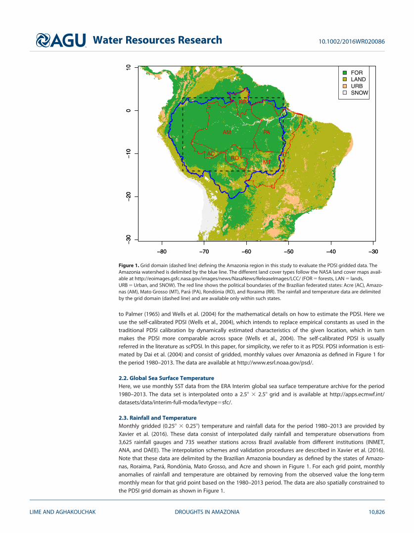
Figure 1. Grid domain (dashed line) defining the Amazonia region in this study to evaluate the PDSI gridded data. TheAmazonia watershed is delimited by the blue line. The different land cover types follow the NASA land cover maps avail-able at http://eoimages.gsfc.nasa.gov/images/news/NasaNews/ReleaseImages/LCC/ (FOR 5 forests, LAN 5 lands,URB 5 Urban, and SNOW). The red line shows the political boundaries of the Brazilian federated states: Acre (AC), Amazo-nas (AM), Mato Grosso (MT), Par�a (PA), Rondonia (RO), and Roraima (RR). The rainfall and temperature data are delimitedby the grid domain (dashed line) and are available only within such states.

Water Resources Research 10.1002/2016WR020086

LIME AND AGHAKOUCHAK DROUGHTS IN AMAZONIA 10,826

3. Spatiotemporal Variability of Drought

The spatiotemporal dynamics of PDSI is first investigated using the principal component analysis (PCA, seeJolliffe, 2002 for more details) based on the centered and scaled PDSI data. The first three principal compo-nents (PCs) respond to 27%, 16%, and 11% of the data variability, respectively. Collectively, they explain54% of the PDSI variance and, given that further components explain, individually, less than 6% of the datavariance, we restrict our analysis to these first three PCs. Figure 2 shows the time series of these first threeleading modes. In order to highlight the most extreme events, the PC values above the 90% and below the10% empirical percentiles are colored in blue and red, respectively.

Based on the PC loadings (eigenvectors) associated with each mode (Figure 3), we can shed some light onthe spatial patterns of droughts in Amazonia. The first mode (top plot of Figure 3) has positive loadingsacross the entire Amazonia, with slightly higher values in the central eastern region. This mode thus repre-sents large droughts in Amazonia and if we consider the extreme events below the 10% percentile, thesedroughts took place in 1983, 1992, 1997–1998, and 2005 (top plot of Figure 2 and Figure 4). The secondmode has a north-south (or meridional) kind of seesaw structure, with dry (wet) conditions south of about68S and wet (dry) conditions north of that latitude. Droughts with such pattern happened in severalmoments in the past (middle plot of Figure 2 and Figure 4), but it is worth mentioning the drought eventsin southern Amazonia that took place in 1988–1989, 2000, 2007, and 2010–2011. Some of these droughtshave been identified in other studies (e.g., Marengo & Espinoza, 2016). In particular, referring to these twofirst modes, the 2005 and 2010 droughts are discussed in the next section. The third mode has a zonal typeof dipole structure (bottom plot of Figure 3). In the following sections, we show that this third mode is

1980 1985 1990 1995 2000 2005 2010 2015−15

−10

−5

0

5

10

Year

PC

1980 1985 1990 1995 2000 2005 2010 2015

−5

0

5

10

Year

PC

1980 1985 1990 1995 2000 2005 2010 2015

−5

0

5

Year

PC

Figure 2. Time series of PDSI principal components (top three, from top to bottom plots). The blue and red colors identifypoints above and below the 90% and 10% percentiles, respectively.

Water Resources Research 10.1002/2016WR020086

LIME AND AGHAKOUCHAK DROUGHTS IN AMAZONIA 10,827

possibly associated with internal and local dynamics rather than large-scale climate processes. Hence, in order to limit the scope of thiswork, we do not analyze droughts associated with this mode as wellas other drought patterns related to the remaining PCs. The specificyears associated with wet events in the first and second PDSI modes(extreme events above the 90% percentile) are available in the sup-porting information.

3.1. Relationship Between PDSI, Rainfall, and TemperatureThe average rainfall and temperature anomalies over the BrazilianAmazonia across the extreme events of the first three leading PDSImodes (Figures 2 and 4) are displayed in Figure 5. The first mode ofPDSI is associated with low rainfall and high temperatures over theentire Amazonia (top plots in Figure 5). Negative anomalies in the sec-ond mode are associated with rainfall below average south of about58S, and slightly positive anomalies in the temperature over westernand southeastern Amazonia and negative anomalies occurring in asmall portion north of 58S and south of about 108S (middle plots inFigure 5). The third mode is associated with low rainfall in easternAmazon and high temperatures in all but a small part in southernAmazonia. This information sheds light on the key drivers of drought,and highlights the role of temperature in Amazonia droughts. We pro-vide in the supporting information the correlation maps between thefirst three leading PDSI modes and rainfall and temperature, andthe conclusions are similar to those obtained for the composites(Figure 5). As shown, temperature plays a major role in droughts anddeserves more attention, especially in light of the projected increasein future temperatures.

4. Drought Teleconnections With Global Sea SurfaceTemperature

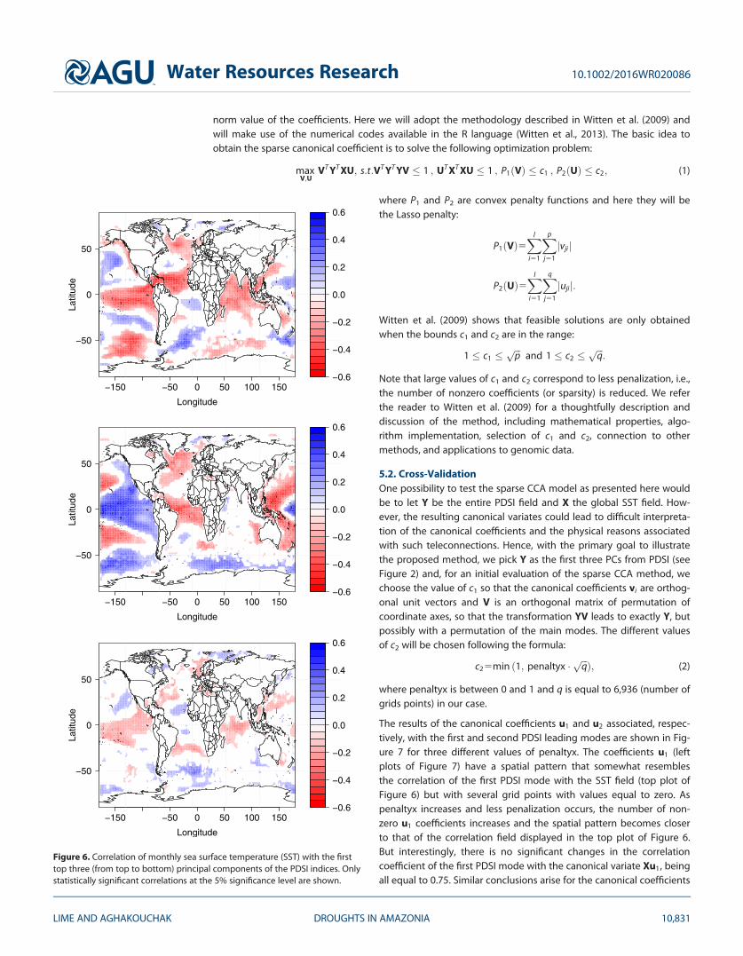
The concurrent correlations of global sea surface temperature (SST)with the first three principal modes of PDSI are shown in Figure 6. Thefirst mode has strong negative correlations in the ENSO region and inthe extratropical South Pacific. This means that the positive anomaliesin these regions are associated with negative anomalies in the firstPDSI mode (i.e., drought conditions across the entire Amazonia). Thispattern along with the negative correlations found in the tropicalNorth Atlantic are related to major droughts in Amazonia (Jim�enez-Mu~noz et al., 2016; Marengo, 1992; Marengo & Espinoza, 2016; Yoon &Zeng, 2010; Zou et al., 2016). Other regions in the North Atlantic andover the entire Indian Ocean present statistically significant correla-tions but potential teleconnection mechanisms with Amazoniadroughts are poorly understood and need further investigations.

The second mode (middle plot in Figure 6) displays a dipole kind ofstructure with the SST field across the Pacific basin, with positive cor-relations in the eastern part and negative correlations in the far west-ern region. The tropical Atlantic shows negative correlations. Thesetwo patterns of correlations suggest that, based on the loadings ofthe second mode (Figure 3), droughts in southern (northern) Amazo-nia as shown in the middle plots of Figure 5 tend to be associatedwith negative (positive) or neutral anomalies in the SST across theENSO region and positive (negative) anomalies in the tropical Atlantic.

−0.2

−0.1

0.0

0.1

0.2

0.02

0.04

0.04

0.06

0.06

0.08

0.08

0.1

0.1

0.12

0.1

2

0.1

4 0

.16

0.1

8

−70 −65 −60 −55

−12

−10

−8

−6

−4

−2

0

Longitude

Latit

ude

−0.2

−0.1

0.0

0.1

0.2

−0.

15

−0.15

−0.

1

−0.1

−0.

05

0

0.05

0.1

0.15

0.2

−70 −65 −60 −55

−12

−10

−8

−6

−4

−2

0

Longitude

Latit

ude

−0.2

−0.1

0.0

0.1

0.2

−0.2

−0.

15

−0.

15

−0.1

−0.

05

0

0.0

5

0.1

0.1

−70 −65 −60 −55

−12

−10

−8

−6

−4

−2

0

Longitude

Latit

ude

Figure 3. Top three (from top to bottom) loadings of PCA applied to the PDSIindices.

Water Resources Research 10.1002/2016WR020086

LIME AND AGHAKOUCHAK DROUGHTS IN AMAZONIA 10,828

Positive correlations are also found in the extratropical North Atlantic,but it is unclear the physical mechanisms responsible for suchteleconnection.

A somehow similar conclusion was described by Zou et al. (2016),which suggested that droughts in northern Amazonia are influencedby El Ni~no events while dry periods in southern Amazonia are relatedto positive SST anomalies in the North Atlantic. They identified the2005 drought as an event that hit southern Amazonia, while the 2010drought was initially started in northern Amazonia and progressivelyhit southern Amazonia due to positive SST anomalies in the NorthAtlantic. Using the results obtained for the first two leading PDSImodes, we offer a slightly different but also complementary view ofthe 2005 and 2010 drought events. The 2005 drought started insouthern Amazonia as identified by the negative anomalies in the sec-ond PDSI mode (Figure 4), and progressively hit the entire region(positive anomalies in the first PDSI mode, Figures 2 and 4). Thedrought event ended with dry conditions in southern Amazonia inthe late 2005 and early 2006 (Figure 4). The 2010 drought eventstarted in northern Amazonia in late 2009 as identified by positive

anomalies in the second PDSI mode (middle plot of Figure 2), then the dry conditions moved to southernAmazonia (Figures 2 and 4) and eventually hit the entire region in September–October 2010. These dry con-ditions had persisted in southern Amazonia until May 2011.

Finally, the third model displays (bottom plot of Figure 6) weaker correlations in several areas across theglobe, with a more remarkable negative correlation region in the tropical Pacific centered around 1508W,suggesting that positive SST anomalies in this region tend to be associated with droughts in the easternAmazonia, as shown in the bottom plots of Figure 5. However, based on the forecast results described inthe next section, we believe that such large-scale teleconnections might play just a minor role on this thirdmode of variability.

5. A Drought Prediction Model for Amazonia

5.1. Technical ApproachBased on the field correlations (see Figure 6), our main goal here is to obtain SST predictors for the PDSImodes in order to provide forecasts at different lead times. Clearly, the maps show several locations thatcould be of just spurious correlations, which, although statistically significant, could be obtained just bychance or be associated with cross correlations within the SST field. The main objective is then to select justa few regions and grid points to obtain more robust SST predictors for the PDSI field.

Here, we propose using the canonical correlation analysis (CCA, see Hotelling, 1936 for the original idea) forlinking SST to PDSI fields in order to obtain highly correlated response and predictor variables in a subspacespanned by such fields (see, e.g., Barnett & Preisendorfer, 1987; Barnston & Ropelewski, 1992). However, theassociated standard CCA transformation is performed through full matrices (with nonzero entries) multipli-cation, which tends to carry a significant amount of noise and less robust estimators in the prediction space.This drawback is usually seen when cross-validated predictions (with out-of-sample data) have limited skillsas compared with high correlations found during the estimation phase. Our idea is to obtain SST predictorsbased on just a few number of grid points in order to avoid excessive noise in the predictor space. In otherwords, we want to find sparse SST grid points in Figure 6 that will lead to skillfully predictors for the PDSImodes. Our approach will follow then the ideas of sparse loadings originally developed for principal compo-nent analysis (e.g., Zou et al., 2006) and further extended to canonical correlation analysis (e.g., Witten et al.,2009). These approaches are also referred as robust (or regularized) methods for principal/canonical correla-tion analysis (e.g., Cand�es et al., 2011; Dehon et al., 2000; Hardoon & Shawe-Taylor, 2011; Jolliffe et al., 2003;Shen & Huang, 2008; Wang & Huang, 2016) and have been developed focused mainly on machine learningproblems and applications. Only recently such specific methods have been explored in hydroclimate appli-cations (Ho et al., 2016).

2 4 6 8 10 12

1980

1990

2000

2010

Month

Year

Figure 4. Periods of dry events (points below the 10% percentile) as identifiedfor the first (black dots) and second (open circles) PDSI principal components.

Water Resources Research 10.1002/2016WR020086

LIME AND AGHAKOUCHAK DROUGHTS IN AMAZONIA 10,829

Let then Y be the n by p matrix of the observed PDSI field over Amazonia (Figure 1), where n 5 408 months(period 1980–2013) and p 5 70 grid points. Let X be the n by q matrix of the global SST field, where q isequal to 6,936 grids points. For simplicity, let us assume that Y and X are centered and scaled matrices. Thebasic idea from canonical correlation analysis originally proposed by Hotelling (1936) is to find two sets ofbasis vectors V and U such that the correlations of projections of Y and X onto these basis vectors (Y V andX U) are maximized. V5½v1 . . . vl� and U5½u1 . . . ul� are the so-called canonical vectors (or weights, coeffi-cients), where vi; i51; . . . ; l, is a column vector with dimension p, ui is a column vector with dimension qand l5min ðp; qÞ. The projections Y vi and X ui onto the coefficients are called canonical variates and, whilethe (canonical) correlation between each pair Y vi and Xui is maximized and decreases from i 5 1 to i 5 l,the cross canonical variates are uncorrelated, i.e., the correlation of Y vi and Xuj is equal to zero for i 6¼ j.

The canonical coefficients V and U will likely have nonzero coefficients on all l variables, and this issuemakes the method less robust to noise in the data and consequently with reduced cross-validated skillwhen one intends to predict Y from X. In order to obtain robust estimates for V and U that are less sensitiveto noise, we will search for sparse vectors V and U such that a certain number of coefficients will be exactlyequal to zero. This can be done by penalizing the canonical vectors in a procedure similar to the LASSO andRIDGE regressions (Hastie et al., 2001), in which a bound is introduced in the sum of the absolute or squared

−100

−50

0

50

100

0

0

−70 −65 −60 −55

−10

−5

0

Longitude

Latit

ude

−0.5

0.0

0.5

1.0

−70 −65 −60 −55

−10

−5

0

Longitude

Latit

ude

−100

−50

0

50

100

0

0 0

0 0

0

0

0

0

0

0

0

0

0

0

−70 −65 −60 −55

−10

−5

0

Longitude

Latit

ude

−0.5

0.0

0.5

1.0

0 0

0

0

0

0

−70 −65 −60 −55

−10

−5

0

Longitude

Latit

ude

−100

−50

0

50

100

0

0

0

0

0

0

0

0

0

0

0

0

0

0

0

0

−70 −65 −60 −55

−10

−5

0

Longitude

Latit

ude

−0.5

0.0

0.5

1.0

0 0

0

0

−70 −65 −60 −55

−10

−5

0

Longitude

Latit

ude

Figure 5. Composite analysis of anomalies in rainfall (left plots, scale in mm) and temperature (right plots, scale in 8C) forthe dry events of the top three (from top to bottom) PDSI principal components.

Water Resources Research 10.1002/2016WR020086

LIME AND AGHAKOUCHAK DROUGHTS IN AMAZONIA 10,830

norm value of the coefficients. Here we will adopt the methodology described in Witten et al. (2009) andwill make use of the numerical codes available in the R language (Witten et al., 2013). The basic idea toobtain the sparse canonical coefficient is to solve the following optimization problem:

maxV;U

VT YT XU; s:t:VT YT YV � 1 ; UT XT XU � 1 ; P1ðVÞ � c1 ; P2ðUÞ � c2; (1)

where P1 and P2 are convex penalty functions and here they will bethe Lasso penalty:

P1ðVÞ5Xl

i51

Xp

j51

jvjij

P2ðUÞ5Xl

i51

Xq

j51

jujij:

Witten et al. (2009) shows that feasible solutions are only obtainedwhen the bounds c1 and c2 are in the range:

1 � c1 �ffiffiffipp

and 1 � c2 �ffiffiffiqp

:

Note that large values of c1 and c2 correspond to less penalization, i.e.,the number of nonzero coefficients (or sparsity) is reduced. We referthe reader to Witten et al. (2009) for a thoughtfully description anddiscussion of the method, including mathematical properties, algo-rithm implementation, selection of c1 and c2, connection to othermethods, and applications to genomic data.

5.2. Cross-ValidationOne possibility to test the sparse CCA model as presented here wouldbe to let Y be the entire PDSI field and X the global SST field. How-ever, the resulting canonical variates could lead to difficult interpreta-tion of the canonical coefficients and the physical reasons associatedwith such teleconnections. Hence, with the primary goal to illustratethe proposed method, we pick Y as the first three PCs from PDSI (seeFigure 2) and, for an initial evaluation of the sparse CCA method, wechoose the value of c1 so that the canonical coefficients vi are orthog-onal unit vectors and V is an orthogonal matrix of permutation ofcoordinate axes, so that the transformation YV leads to exactly Y, butpossibly with a permutation of the main modes. The different valuesof c2 will be chosen following the formula:

c25min 1; penaltyx � ffiffiffiqpð Þ; (2)

where penaltyx is between 0 and 1 and q is equal to 6,936 (number ofgrids points) in our case.

The results of the canonical coefficients u1 and u2 associated, respec-tively, with the first and second PDSI leading modes are shown in Fig-ure 7 for three different values of penaltyx. The coefficients u1 (leftplots of Figure 7) have a spatial pattern that somewhat resemblesthe correlation of the first PDSI mode with the SST field (top plot ofFigure 6) but with several grid points with values equal to zero. Aspenaltyx increases and less penalization occurs, the number of non-zero u1 coefficients increases and the spatial pattern becomes closerto that of the correlation field displayed in the top plot of Figure 6.But interestingly, there is no significant changes in the correlationcoefficient of the first PDSI mode with the canonical variate Xu1, beingall equal to 0.75. Similar conclusions arise for the canonical coefficients

−0.6

−0.4

−0.2

0.0

0.2

0.4

0.6

−150 −50 0 50 100 150

−50

0

50

Longitude

Latit

ude

−0.6

−0.4

−0.2

0.0

0.2

0.4

0.6

−150 −50 0 50 100 150

−50

0

50

Longitude

Latit

ude

−0.6

−0.4

−0.2

0.0

0.2

0.4

0.6

−150 −50 0 50 100 150

−50

0

50

Longitude

Latit

ude

Figure 6. Correlation of monthly sea surface temperature (SST) with the firsttop three (from top to bottom) principal components of the PDSI indices. Onlystatistically significant correlations at the 5% significance level are shown.

Water Resources Research 10.1002/2016WR020086

LIME AND AGHAKOUCHAK DROUGHTS IN AMAZONIA 10,831

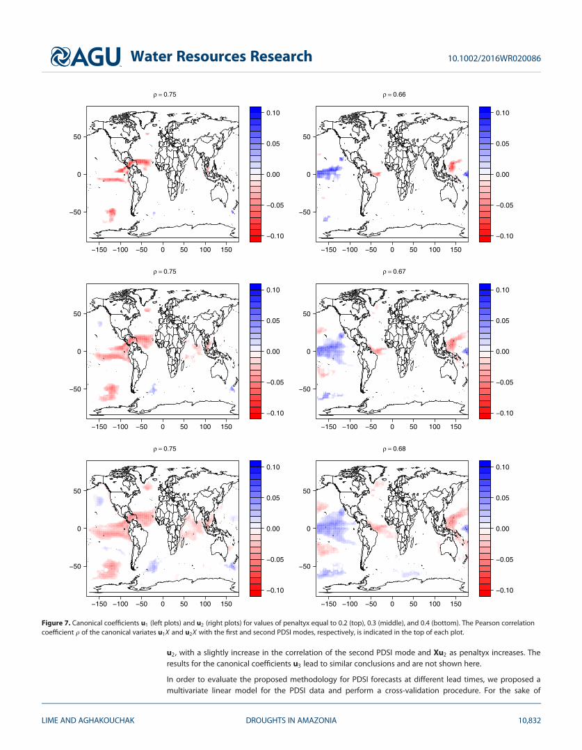
u2, with a slightly increase in the correlation of the second PDSI mode and Xu2 as penaltyx increases. Theresults for the canonical coefficients u3 lead to similar conclusions and are not shown here.

In order to evaluate the proposed methodology for PDSI forecasts at different lead times, we proposed amultivariate linear model for the PDSI data and perform a cross-validation procedure. For the sake of

−0.10

−0.05

0.00

0.05

0.10

−150 −100 −50 0 50 100 150

−50

0

50

ρ = 0.75

−0.10

−0.05

0.00

0.05

0.10

−150 −100 −50 0 50 100 150

−50

0

50

ρ = 0.66

−0.10

−0.05

0.00

0.05

0.10

−150 −100 −50 0 50 100 150

−50

0

50

ρ = 0.75

−0.10

−0.05

0.00

0.05

0.10

−150 −100 −50 0 50 100 150

−50

0

50

ρ = 0.67

−0.10

−0.05

0.00

0.05

0.10

−150 −100 −50 0 50 100 150

−50

0

50

ρ = 0.75

−0.10

−0.05

0.00

0.05

0.10

−150 −100 −50 0 50 100 150

−50

0

50

ρ = 0.68

Figure 7. Canonical coefficients u1 (left plots) and u2 (right plots) for values of penaltyx equal to 0.2 (top), 0.3 (middle), and 0.4 (bottom). The Pearson correlationcoefficient q of the canonical variates u1X and u2X with the first and second PDSI modes, respectively, is indicated in the top of each plot.

Water Resources Research 10.1002/2016WR020086

LIME AND AGHAKOUCHAK DROUGHTS IN AMAZONIA 10,832

simplicity, we will keep for all lead times tested a fixed value of 0.3 forpenaltyx, which we believe, based on Figure 7, will yield to a good bal-ance between model complexity and model skill. For c1 and the corre-spondent penaltyy (similar to equation (2)), we observed thatpenaltyy 5 0.3 yields to the desired orthogonal matrix V for concurrentY and X. Therefore, for the purpose of this work to illustrate the modelskill, we keep this value also fixed for different lead times, which mightnot lead necessarily to an orthogonal matrix V for all lead times.

Let us assume that Yt is the vector containing the observed values ofthe first three PDSI modes for a given month t. A multivariate linearmodel relating them to past values and to the canonical variatesderived from the SST field is proposed here:

Yt5a1h � Yt2s1b � ðXt2sUÞ1�; (3)

where a is a 3-D vector of intercept terms, h is a 3 3 3 matrix of autore-gressive coefficients, b is a 3 3 3 matrix of exogenous coefficients, � fol-lows a zero-mean multivariate normal distribution with covariance R,and s51; . . . ; 9 is the lead time of the forecast in months.

The skill of the proposed model is evaluated through an 1 year leave-out cross-validation procedure, in which the observations of Y for thefirst year of the record and the associated predictors as depicted in

equation (3) are withdrew, while the data for the remaining years are used to estimate the model parametersa, h, b, and U. The estimated model is then used to predict Y for the first year. The entire procedure is repeateduntil forecasts are made for all years of the record. A baseline model based solely on the autoregressive andintercept terms (i.e., b50 in equation (3)) is used to evaluate the real gain in model skill by including externalinformation based on the SST data and the sparse CCA model. Predictions for the entire PDSI field and the spa-tial average PDSI are also evaluated by taking the predicted PDSI first three modes Y and transforming themback to the original space using the estimated PCA loadings as described in section 3.

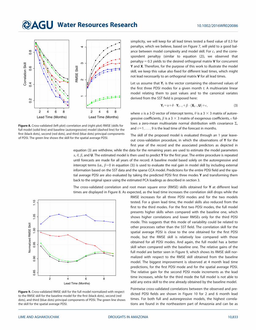
The cross-validated correlation and root mean square error (RMSE) skills obtained for Y at different leadtimes are displayed in Figure 8. As expected, as the lead time increases the correlation skill drops while the

RMSE increases for all three PDSI modes and for the two modelstested. For a given lead time, the model skills also reduced from thefirst to the third modes. For the first two PDSI modes, the full modelpresents higher skills when compared with the baseline one, whichshows higher correlations and lower RMSEs only for the third PDSImode. This suggests that this mode of variability could be related toother processes rather than the SST field. The correlation skill for thespatial average PDSI is close to the one obtained for the first PDSImode, but the RMSE skill is relatively low compared with thoseobtained for all PDSI modes. And again, the full model has a betterskill when compared with the baseline one. The relative gains of thefull model are better seen in Figure 9, which shows its RMSE skill nor-malized with respect to the RMSE skill obtained from the baselinemodel. The biggest improvement is observed at 4 month lead timepredictions, for the first PDSI mode and for the spatial average PDSI.The relative gain for the second PDSI mode increments as the leadtime increases, while for the third mode the full model is not able toadd any extra skill to the one already obtained by the baseline model.

Pointwise cross-validated correlations between the observed and pre-dicted PDSI fields are shown in Figure 10 for 2 and 6 month leadtimes. For both full and autoregressive models, the highest correla-tions are found in the northeastern part of Amazonia and can be as

2 4 6 8

0.2

0.4

0.6

0.8

Lead Time (Months)

Cor

rela

tion

Ski

ll

2 4 6 8

12

34

Lead Time (Months)

RM

SE

Ski

ll

Figure 8. Cross-validated (left plot) correlation and (right plot) RMSE (skills forfull model (solid line) and baseline (autoregressive) model (dashed line) for thefirst (black dots), second (red dots), and third (blue dots) principal componentsof PDSI. The green line shows the skill for the spatial average PDSI.

2 4 6 8

0.85

0.90

0.95

1.00

1.05

1.10

Lead Time (Months)

Nor

mal

ized

RM

SE

Ski

ll

Figure 9. Cross-validated RMSE skill for the full model normalized with respectto the RMSE skill for the baseline model for the first (black dots), second (reddots), and third (blue dots) principal components of PDSI. The green line showsthe skill for the spatial average PDSI.

Water Resources Research 10.1002/2016WR020086

LIME AND AGHAKOUCHAK DROUGHTS IN AMAZONIA 10,833

high as 0.7 for 2 month lead time and 0.6 for 6 month lead time. The difference between the skill of the twomodels is more evident for 6 month lead time.

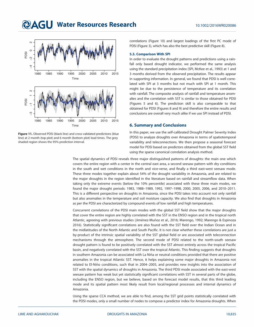
The ability of the full model to predict the spatial average PDSI is also shown in Figure 11 for 2 and 6 monthlead times. Visually, the model is able to predict all the largest drought events with 2 months of anteced-ence and some of the events with 6 month lead time, although the magnitude of such events is underesti-mated in this case. Around 7% of the observed values are outside the 95% prediction intervals.

Finally, in Figure 12, we show the observed PDSI field averaged over the extreme events identified for thefirst and second modes (Figures 4 and 5) and the corresponding predicted PDSI field averaged over thesame events for lead times of 1 and 6 months. In the cases of drought events associated with the first PDSImode (left plots of Figure 12), which correspond to droughts across the entire Amazonia (Figure 5), the pre-diction model is able to highlight the driest region in northeastern Amazonia at 2 month lead time, while at6 month lead time the predictions resemble the observed spatial pattern but underestimate the droughtmagnitude. Droughts related to the second PDSI mode, which features a dipole kind of pattern, with wet(dry) conditions in the north (south) and vice-verse, are also satisfactorily predicted by the proposed modelat both lead times (right plots of Figure 12), particularly in terms of spatial variability. The drought magni-tude is slightly underestimated in both cases.

The gain of the proposed model over climatology (i.e., benchmark model) is finally evaluated through theBrier skill score (Wilks, 2006). For each grid point of PDSI, we consider the 20% most extreme droughts, i.e.,events with a cumulative probability of 20% (climatology). This probability is used to estimate the Brier scorefor the reference model. The Brier score for the proposed model is obtained through the cross-validated pre-dictions by estimating, for each month and grid point, the cumulative probability associated with the respec-tive 20% PDSI quantile obtained from the observed data. The results for 1, 2, 4, and 6 month lead times areshown in Figure 13. The skills are higher in the northeastern region and resembles the region of highest

−0.2

0.0

0.2

0.4

0.6

0.8

1.0

0 4

0.4

0.6

−70 −65 −60 −55

−12

−10

−8

−6

−4

−2

0

Longitude

Latit

ude

−0.2

0.0

0.2

0.4

0.6

0.8

1.0

0.4

0.4

0.4

0.6

0.6

−70 −65 −60 −55

−12

−10

−8

−6

−4

−2

0

Longitude

Latit

ude

−0.2

0.0

0.2

0.4

0.6

0.8

1.0

0

0.2

0.2

0.2

0.2

0.2

0.2

0.2

0.4

0.6

0.6

−70 −65 −60 −55

−12

−10

−8

−6

−4

−2

0

Longitude

Latit

ude

−0.2

0.0

0.2

0.4

0.6

0.8

1.0

0

0.2

0.2

0.4

−70 −65 −60 −55

−12

−10

−8

−6

−4

−2

0

Longitude

Latit

ude

Figure 10. Correlation skill for cross-validated predictions at 2 month (top plots) and 6 month (bottom plots) lead timesobtained from the full (left plots) and autoregressive (right plots) models.

Water Resources Research 10.1002/2016WR020086

LIME AND AGHAKOUCHAK DROUGHTS IN AMAZONIA 10,834

correlations (Figure 10) and largest loadings of the first PC mode ofPDSI (Figure 3), which has also the best predictive skill (Figure 8).

5.3. Comparison With SPIIn order to evaluate the drought patterns and predictions using a rain-fall only based drought indicator, we performed the same analysisusing the standard precipitation index (SPI, McKee et al., 1993) at 1 and3 months derived from the observed precipitation. The results appearin supporting information. In general, we found that PDSI is well corre-lated with SPI at 3 months but not much with SPI at 1 month. Thismight be due to the persistence of temperature and its correlationwith rainfall. The composite analysis of rainfall and temperature anom-alies and the correlation with SST is similar to those obtained for PDSI(Figures 5 and 6). The prediction skill is also comparable to thatobtained for PDSI (Figures 8 and 9) and therefore the entire results andconclusions are overall very much alike if we use SPI instead of PDSI.

6. Summary and Conclusions

In this paper, we use the self-calibrated Drought Palmer Severity Index(PDSI) to analyze droughts over Amazonia in terms of spatiotemporalvariability and teleconnections. We then propose a seasonal forecastmodel for PDSI based on predictors obtained from the global SST fieldusing the sparse canonical correlation analysis method.

The spatial dynamics of PDSI reveals three major distinguished patterns of droughts: the main one whichcovers the entire region with a center in the central east area, a second seesaw pattern with dry conditionsin the south and wet conditions in the north and vice-verse, and finally a third east-west seesaw mode.These three modes together explain about 54% of the drought variability in Amazonia, and are related tothe major droughts in the region identified in the literature based on rainfall and streamflow data. Whentaking only the extreme events (below the 10% percentile) associated with these three main modes, wefound the major drought periods: 1983, 1988–1989, 1992, 1997–1998, 2000, 2005, 2006, and 2010–2011.This is a different perspective on droughts in Amazonia, since the PDSI takes into account not only rainfallbut also anomalies in the temperature and soil moisture capacity. We also find that droughts in Amazoniaas per the PDSI are characterized by compound events of low rainfall and high temperatures.

Concurrent correlations of the PDSI main modes with the global SST field show that the major droughtsthat cover the entire region are highly correlated with the SST in the ENSO region and in the tropical northAtlantic, agreeing with previous studies (Jim�enez-Mu~noz et al., 2016; Marengo, 1992; Marengo & Espinoza2016). Statistically significant correlations are also found with the SST field over the Indian Ocean and inthe midlatitudes of the North Atlantic and South Pacific. It is not clear whether these correlations are just aby-product of the intrinsic spatial variability of the SST global field or are associated with teleconnectionmechanisms through the atmosphere. The second mode of PDSI related to the north-south seesawdrought pattern is found to be positively correlated with the SST almost entirely across the tropical Pacificbasin, and negatively correlated with the SST over the tropical Atlantic. This finding suggests that droughtsin southern Amazonia can be associated with La Ni~na or neutral conditions provided that there are positiveanomalies in the tropical Atlantic SST. Hence, it helps explaining some major droughts in Amazonia notrelated to El-Ni~no conditions, such that in 2004–2005, and provides new insights into the association ofSST with the spatial dynamics of droughts in Amazonia. The third PDSI mode associated with the east-westseesaw pattern has weak but yet statistically significant correlations with SST in several parts of the globe,including the ENSO region, but we believe, based on the forecast model results, that this third leadingmode and its spatial pattern most likely result from local/regional processes and internal dynamics ofAmazonia.

Using the sparse CCA method, we are able to find, among the SST grid points statistically correlated withthe PDSI modes, only a small number of nodes to compose a predictor index for Amazonia droughts. When

Time

PD

SI

1980 1985 1990 1995 2000 2005 2010 2015

−4

−2

02

Time

PD

SI

1980 1985 1990 1995 2000 2005 2010 2015

−3

−1

12

Figure 11. Observed PDSI (black line) and cross-validated predictions (blueline) at 2 month (top plot) and 6 month (bottom plot) lead times. The greyshaded region shows the 95% prediction interval.

Water Resources Research 10.1002/2016WR020086

LIME AND AGHAKOUCHAK DROUGHTS IN AMAZONIA 10,835

compared to an autoregressive baseline model, the inclusion of these exogenous predictors in a forecastmodel for PDSI leads to an increase in the forecast skill. In a cross-validation procedure, we obtain correla-tions between the observed and predicted spatially average PDSI up to 0.60 and 0.45 for lead times of 5and 9 months, respectively. These values are in the same order of magnitude or even above correlationsobtained from more complex models developed for drought and El Ni~no predictions (e.g., Barnston et al.,2012; Thober et al., 2015). The proposed model is also able to satisfactorily predict the spatial variability of

−4

−2

0

2

4

−4

−3

−3

−2

−2

−2

−1

−1

0

2

−70 −65 −60 −55

−12

−10

−8

−6

−4

−2

0

Longitude

Latit

ude

−4

−2

0

2

4

−4

−3

−2

−2

−1

0

0

1

1

2

3

−70 −65 −60 −55

−12

−10

−8

−6

−4

−2

0

Longitude

Latit

ude

−4

−2

0

2

4 −3

−3

−2

−2

−2

−2

−2

−1

−1

0

2

−70 −65 −60 −55

−12

−10

−8

−6

−4

−2

0

Longitude

Latit

ude

−4

−2

0

2

4

−3

−2

−2

−1

−1

0

0

1

1

2

3

−70 −65 −60 −55

−12

−10

−8

−6

−4

−2

0

Longitude

Latit

ude

−4

−2

0

2

4

−2.5

−2

−2

−1.5

−1.

5

−1

−1

−1

−1

−1

−0.5

−0.5

−

0.5

0

0.5

1.5

−70 −65 −60 −55

−12

−10

−8

−6

−4

−2

0

Longitude

Latit

ude

−4

−2

0

2

4

−2

−1.

5

5.1

−

−1

−1

−0.

5

−0.5

−0.5

0

0

0.5 0

.5

0.5

0.5

1

1

1

1.5

−70 −65 −60 −55

−12

−10

−8

−6

−4

−2

0

Longitude

Latit

ude

Figure 12. Composite analysis of extreme droughts in the first (left plots) and second (right plots) PC from PDSI. The topplots show observed values while the predictions at 2 month and 6 month lead times are shown in the middle and bot-tom plots, respectively.

Water Resources Research 10.1002/2016WR020086

LIME AND AGHAKOUCHAK DROUGHTS IN AMAZONIA 10,836

PDSI, although the magnitude is generally underestimated. The gain over climatology, as evaluated by theBrier skill score, is on average 20% for 1 month and 2% for 6 month lead times, although values up to 58%are obtained in the northeastern region of Amazonia.

To the best of our knowledge, the Amazonia drought forecast model proposed here is the first in the litera-ture to provide, based on cross-validation results, satisfactory skills for lead times beyond 4 months. Further-more, the approach offers the potential to capture the spatial variability of Amazonia droughts. The modelis relatively easy to implement and can be used in operational mode as a tool for risk assessment in Amazo-nia, integrating Brazilian initiatives of drought monitor systems (e.g., the INPE drought monitor at http://clima1.cptec.inpe.br/spi/pt and the FUNCEME drought monitor at http://msne.funceme.br/). The inferenceprocess of the proposed model considered the penalization parameter of the sparse CCA constant acrossthe different lead times, and this is one aspect that can be improved in future studies. Moreover, other cli-mate variables such as sea level pressure and geopotential height fields can be added to the model topotentially improve the forecast skills, particularly at short lead times, and with time varying coefficients.The PDSI shows high correlations with rainfall across Amazonia but the possibility to use other drought indi-ces (e.g., Hao & Singh 2015; Mishra & Singh, 2010; Mu et al., 2013; Rajsekhar et al., 2015; Shukla & Wood2008) to better represent dry conditions in the region could be also explored in future studies. Finally, webelieve the results obtained and the model proposed in this work are a step forward to improve the man-agement of drought impacts in Amazonia, including the local and regional societal impacts, water resour-ces, and the ecosystem response.

−0.2

0.0

0.2

0.4

0.6

0

0

0

0

0

0.2

0.2

0.2

0.2

0.4

0.4

−70 −65 −60 −55

−12

−10

−8

−6

−4

−2

0

a)

Longitude

Latit

ude

< 0.19>

−0.2

0.0

0.2

0.4

0.6

0

0

0

0

0.2

0.2

0.2

2.0

0.4

0.4

−70 −65 −60 −55

−12

−10

−8

−6

−4

−2

0

b)

Longitude

Latit

ude

< 0.15>

−0.2

0.0

0.2

0.4

0.6

0

0

0

0

0

0.2

0.4

−70 −65 −60 −55

−12

−10

−8

−6

−4

−2

0

c)

Longitude

Latit

ude

< 0.08>

−0.2

0.0

0.2

0.4

0.6

0 2

−0.

2

0

0

0

0

0.2

−70 −65 −60 −55

−12

−10

−8

−6

−4

−2

0

d)

Longitude

Latit

ude

< 0.02>

Figure 13. Brier skill score for (a) 1 month, (b) 2 month, (c) 4 month, and (d) 6 month lead times. The spatial average ofthe corresponding score is shown in the top right corner of the plots.

Water Resources Research 10.1002/2016WR020086

LIME AND AGHAKOUCHAK DROUGHTS IN AMAZONIA 10,837

ReferencesAghaKouchak, A., Cheng, L., Mazdiyasni, O., & Farahmand, A. (2014). Global warming and changes in risk of concurrent climate extremes:

Insights from the 2014 California drought. Geophysical Research Letters, 41, 8847–8852. https://doi.org/10.1002/2014GL062308Alley, W. M. (1984). The Palmer drought severity index: Limitations and assumptions. Journal of Climate and Applied Meteorology, 23(7),

1100–1109. https://doi.org/10.1175/1520-0450(1984)023<1100: TPDSIL>2.0.CO;2Arag~ao, L. E. O. C., Malhi, Y., Roman-Cuesta, R. M., Saatchi, S., Anderson, L. O., & Shimabukuro, Y. E. (2007). Spatial patterns and fire response

of recent Amazonian droughts. Geophysical Research Letters, 34, L07701. https://doi.org/10.1029/2006GL028946Arraut, J. M., Nobre, C., Barbosa, H. M. J., Obregon, G., & Maregon, J. (2012). Aerial rivers and lakes: Looking at large-scale moisture transport

and its relation to Amazonia and to subtropical rainfall in South America. Journal of Climate, 25, 543–556.Barnett, T. P., & Preisendorfer, R. (1987). Origins and levels of monthly and seasonal forecast skill for United States surface air temperatures

determined by canonical correlation analysis. Monthly Weather Review, 115(9), 1825–1850. https://doi.org/10.1175/1520-0493(1987)115<1825:OALOMA>2.0.CO;2

Barnston, A. G., & Ropelewski, C. F. (1992). Prediction of ENSO episodes using canonical correlation analysis. Journal of Climate, 5(11), 1316–1345. https://doi.org/10.1175/1520-0442(1992)005<1316:POEEUC>2.0.CO;2

Barnston, A. G., Tippett, M. K., L’Heureux, M. L., Li, S., & DeWitt, D. G. (2012). Skill of real-time seasonal ENSO model predictions during2002–11: Is our capability increasing? Bulletin of the American Meteorological Society, 93(5), 631–651. https://doi.org/10.1175/BAMS-D-11-00111.1

Cand�es, E. J., Li, X., Ma, Y., & Wright, J. (2011). Robust principal component analysis? Journal of ACM, 58(3), 11:1–11:37. https://doi.org/10.1145/1970392.1970395

Chen, Y., Morton, D. C., Jin, Y., Collatz, G. J., Kasibhatla, P. S., van der Werf, G. R., . . . Randerson, J. T. (2013). Long-term trends and interan-nual variability of forest, savanna and agricultural fires in South America. Carbon Management, 4(6), 617–638. https://doi.org/10.4155/cmt.13.61

Cochrane, M. A. (2003). Fire science for rainforests. Nature, 421, 913–919. https://doi.org/10.1038/nature01437Cook, E. R., Seager, R., Heim, R. R., Vose, R. S., Herweijer, C., & Woodhouse, C. (2010). Megadroughts in North America: Placing IPCC projec-

tions of hydroclimatic change in a long-term palaeoclimate context. Journal of Quaternary Science, 25(1), 48–61. https://doi.org/10.1002/jqs.1303

Dai, A. (2011). Characteristics and trends in various forms of the Palmer drought severity index during 1900–2008. Journal of GeophysicalResearch, 116, D12115. https://doi.org/10.1029/2010JD015541

Dai, A., Trenberth, K. E., & Qian, T. (2004). A global data set of palmer drought severity index for 1870–2002: Relationship with soil moistureand effects of surface warming. Journal of Hydrometeorology, 5, 1117–1130.

Dehon, C., Filzmoser, P., & Croux, C. (2000). Robust methods for canonical correlation analysis (pp. 321–326). Berlin, Heidelberg: Springer.https://doi.org/10.1007/978-3-642-59789-3_51

Drumond, A., Nieto, R., Gimeno, L., & Ambrizzi, T. (2008). A Lagrangian identification of major sources of moisture over Central Brazil and LaPlata Basin. Journal of Geophysical Research, 113, D14128. https://doi.org/10.1029/2007JD009547

Espinoza, J. C., Ronchail, J., Guyot, J.-L., Junquas, C., Vauchel, P., Lavado, W., . . . Pombosa, R. (2011). Climate variability and extreme droughtin the upper Solimoes River (western Amazon Basin): Understanding the exceptional 2010 drought. Geophysical Research Letters, 38,L13406. https://doi.org/10.1029/2011gl047862

Feldpausch, T. R., Phillips, O. L., Brienen, R. J. W., Gloor, E., Lloyd, J., Lopez-Gonzalez, G., . . . Vos, R. . . . (2016). Amazon forest response torepeated droughts. Global Biogeochemical Cycles, 30, 964–982. https://doi.org/10.1002/2015GB005133

Fernandes, K., Giannini, A., Verchot, L., Baethgen, W., & Pinedo-Vasquez, M. (2015). Decadal covariability of Atlantic SSTs and western Ama-zon dry-season hydroclimate in observations and CMIP5 simulations. Geophysical Research Letters, 42, 6793–6801. https://doi.org/10.1002/2015GL063911, 2015GL063911.

Funk, C., Hoell, A., Shukla, S., Blad�e, I., Liebmann, B., Roberts, J. B., . . . Husak, G. (2014). Predicting east African spring droughts using Pacificand Indian Ocean sea surface temperature indices. Hydrology and Earth System Sciences, 18(12), 4965–4978. https://doi.org/10.5194/hess-18-4965-2014

Hao, Z., & AghaKouchak, A. (2014). A nonparametric multivariate multi-index drought monitoring framework. Journal of Hydrometeorology,15(1), 89–101. https://doi.org/10.1175/JHM-D-12-0160.1

Hao, Z., & Singh, V. P. (2015). Drought characterization from a multivariate perspective: A review. Journal of Hydrology, 527, 668–678.https://doi.org/10.1016/j.jhydrol.2015.05.031

Hardoon, D. R., & Shawe-Taylor, J. (2011). Sparse canonical correlation analysis. Machine Learning, 83(3), 331–353. https://doi.org/10.1007/s10994-010-5222-7

Hastie, T., Tibshirani, R., & Friedman, J. (2001). The elements of statistical learning. Berlin, Germany: Springer.Hayes, M. J., Svoboda, M. D., Wilhite, D. A., & Vanyarkho, O. V. (1999). Monitoring the 1996 drought using the standardized precipitation

index. Bulletin of the American Meteorological Society, 80(3), 429–438. https://doi.org/10.1175/1520-0477(1999)080<0429:MTDUTS>2.0.CO;2

Heim, R. R. Jr, (2002). A review of twentieth-century drought indices used in the United States. Bulletin of the American Meteorological Soci-ety, 83, 1149–1165.

Ho, M., Lall, U., & Cook, E. R. (2016). Can a paleodrought record be used to reconstruct streamflow? A case study for the Missouri RiverBasin. Water Resources Research, 52, 5195–5212. https://doi.org/10.1002/2015WR018444

Hoerling, M., Eischeid, J., Perlwitz, J., Quan, X., Zhang, T., & Pegion, P. (2012). On the increased frequency of Mediterranean drought. Journalof Climate, 25(6), 2146–2161. https://doi.org/10.1175/JCLI-D-11-00296.1

Hotelling, H. (1936). Relations between two sets of variates. Biometrika, 28, 321–377.Jim�enez-Mu~noz, J. C., Mattar, C., Barichivich, J., Santamar�ıa-Artigas, A., Takahashi, K., Malhi, Y., . . . van der Schrier, G. (2016). Record-breaking

warming and extreme drought in the Amazon rainforest during the course of El Ni~no 2015–2016. Scientific Reports, 6, 33130. https://doi.org/10.1038/srep33130

Joetzjer, E., Douville, H., Delire, C., Ciais, P., Decharme, B., & Tyteca, S. (2013). Hydrologic benchmarking of meteorological drought indicesat interannual to climate change timescales: A case study over the Amazon and Mississippi river basins. Hydrology and Earth System Sci-ences, 17(12), 4885–4895. https://doi.org/10.5194/hess-17-4885-2013

Jolliffe, I. T. (2002). Principal component analysis (2nd ed.). New York, NY: Springer-Verlag.Jolliffe, I. T., Trendafilov, N. T., & Uddin, M. (2003). A modified principal component technique based on the LASSO. Journal of Computa-

tional and Graphical Statistics, 12(3), 531–547.

AcknowledgmentsWe thank the Associate Editor and theanonymous reviewers for theirconstructive criticism that greatlyimproved the original manuscript. Thefirst author acknowledges aPostdoctoral Fellowship from theBrazilian Government Agency CNPqduring part of this work. The secondauthor was partially supported by theNational Aeronautics and SpaceAdministration (NASA) awardNNX15AC27G and National Oceanicand Atmospheric Administration(NOAA) award NA14OAR4310222. TheDai Palmer Drought Severity Index(PDSI) data are provided by the NOAA/OAR/ESRL PSD, Boulder, CO, USA, fromtheir Web site at http://www.esrl.noaa.gov/psd/. Sea surface temperaturedata are obtained at http://apps.ecmwf.int/datasets/data/interim-full-moda/levtype5sfc/. Rainfall andtemperature data are provided byXavier et al. (2016). We thank all theagencies and authors that providedata set and codes.

Water Resources Research 10.1002/2016WR020086

LIME AND AGHAKOUCHAK DROUGHTS IN AMAZONIA 10,838

Keyantash, J., & Dracup, J. A. (2002). The quantification of drought: An evaluation of drought indices. Bulletin of the American MeteorologicalSociety, 83, 1167–1180.

Kwon, H.-H., Lall, U., & Kim, S.-J. (2016). The unusual 2013–2015 drought in South Korea in the context of a multicentury precipitationrecord: Inferences from a nonstationary, multivariate, Bayesian copula model. Geophysical Research Letters, 43, 8534–8544. https://doi.org/10.1002/2016GL070270

Laurance, W. F., & Williamson, G. B. (2001). Positive feedbacks among forest fragmentation, drought, and climate change in the Amazon.Conservation Biology, 15(6), 1529–1535. https://doi.org/10.1046/j.1523-1739.2001.01093.x

Lopes, A. V., Chiang, J. C. H., Thompson, S. A., & Dracup, J. A. (2016). Trend and uncertainty in spatial-temporal patterns of hydrologicaldroughts in the Amazon basin. Geophysical Research Letters, 43, 3307–3316. https://doi.org/10.1002/2016GL067738

Lyon, B., Bell, M. A., Tippett, M. K., Kumar, A., Hoerling, M. P., Quan, X.-W., & Wang, H. (2012). Baseline probabilities for the seasonal predictionof meteorological drought. Journal of Applied Meteorology and Climatology, 51(7), 1222–1237. https://doi.org/10.1175/JAMC-D-11-0132.1

Maeda, E. E., Kim, H., Arag~ao, L. E. O. C., Famiglietti, J. S., & Oki, T. (2015). Disruption of hydroecological equilibrium in southwest Amazonmediated by drought. Geophysical Research Letters, 42, 7546–7553. https://doi.org/10.1002/2015GL065252

Marengo, J. A. (1992). Interannual variability of surface climate in the Amazon basin. International Journal of Climatology, 12(8), 853–863.https://doi.org/10.1002/joc.3370120808

Marengo, J. A., & Espinoza, J. C. (2016). Extreme seasonal droughts and floods in Amazonia: Causes, trends and impacts. International Jour-nal of Climatology, 36, 1033–1050.

Marengo, J. A., Nobre, C. A., Tomasella, J., Cardoso, M., & Oyama, M. (2008a). Hydro-climate and ecological behaviour of the drought ofAmazonia in 2005. Philosophical Transactions of the Royal Society of London. Series B, Biological Sciences, 363(1498), 1773–1778. https://doi.org/10.1098/rstb.2007.0015

Marengo, J. A., Nobre, C. A., Tomasella, J., Oyama, M. D., Oliveira, G. S. D., Oliveira, R. D., . . . Brown, I. F. (2008b). The drought of Amazonia in2005. Journal of Climate, 21(3), 495–516. https://doi.org/10.1175/2007JCLI1600.1

Marengo, J. A., Tomasella, J., Alves, L. M., Soares, W. R., & Rodriguez, D. A. (2011). The drought of 2010 in the context of historical droughtsin the Amazon region. Geophysical Research Letters, 38, L12703. https://doi.org/10.1029/2011GL047436

McClain, M. E., Victoria, R., & Richey, J. E. (2001). The biogeochemistry of the Amazon basin (384 p.). Oxford, UK: Oxford University Press.McKee, T. B., Doesken, N. J., & Kleist, J. (1993). The relationship of drought frequency and duration of time scales. In Eighth conference on

applied climatology (pp. 179–186). Anaheim, CA: American Meteorological Society.Mishra, A. K., & Singh, V. P. (2010). A review of drought concepts. Journal of Hydrology, 391(1–2), 202–216. https://doi.org/10.1016/j.jhydrol.

2010.07.012Mu, Q., Zhao, M., Kimball, J. S., McDowell, N. G., & Running, S. W. (2013). a remotely sensed global terrestrial drought severity index. Bulletin

of the American Meteorological Society, 94(1), 83–98. https://doi.org/10.1175/BAMS-D-11-00213.1Nobre, C. A., Sellers, P. J., & Shukla, J. (1991). Amazonian deforestation and regional climate change. Journal of Climate, 4(10), 957–988.

https://doi.org/10.1175/1520-0442(1991)004<0957:ADARCC>2. 0.CO;2Palmer, W. C. (1965). Meteorological drought (Tech. Rep. 45, 65 p.). Washington, DC: U.S. Weather Bureau.Phillips, O. L., Arag~ao, L. E. O. C., Lewis, S. L., Fisher, J. B., Lloyd, J., L�opez-Gonz�alez, G., Y., . . . Torres-Lezama, A. (2009). Drought sensitivity of

the Amazon rainforest. Science, 323(5919), 1344–1347. https://doi.org/10.1126/science.1164033Rajagopalan, B., Cook, E., Lall, U., & Ray, B. K. (2000). Spatiotemporal variability of ENSO and SST teleconnections to summer drought over

the United States during the twentieth century. Journal of Climate, 13(24), 4244–4255. https://doi.org/10.1175/1520-0442(2000)013<4244:SVOEAS>2.0.CO; 2

Rajsekhar, D., Singh, V. P., & Mishra, A. K. (2015). Multivariate drought index: An information theory based approach for integrated droughtassessment. Journal of Hydrology, 526, 164–182. https://doi.org/10.1016/j.jhydrol.2014.11.031

Ropelewski, C., & Halpert, M. (1987). Global and regional scale precipitation patterns associated with the El Ni~no/southern oscillation.Monthly Weather Review, 115, 1606–1626.

Schubert, S., Koster, R., Hoerling, M., Seager, R., Lettenmaier, D., Kumar, A., & Gutzler, D. (2007). Predicting drought on seasonal-to-decadaltime scales. Bulletin of the American Meteorological Society, 88(10), 1625–1630.

Seager, R., Hoerling, M., Schubert, S., Wang, H., Lyon, B., Kumar, A., . . . Henderson, N. (2015). Causes of the 2011–14 California drought. Jour-nal of Climate, 28(18), 6997–7024. https://doi.org/10.1175/JCLI-D-14-00860.1

Shen, H., & Huang, J. Z. (2008). Sparse principal component analysis via regularized low rank matrix approximation. Journal of MultivariateAnalysis, 99(6), 1015–1034. https://doi.org/10.1016/j.jmva.2007.06.007

Shukla, S., Safeeq, M., AghaKouchak, A., Guan, K., & Funk, C. (2015). Temperature impacts on the water year 2014 drought in California. Geo-physical Research Letters, 42, 4384–4393. https://doi.org/10.1002/2015GL063666

Shukla, S., & Wood, A. W. (2008). Use of a standardized runoff index for characterizing hydrologic drought. Geophysical Research Letters, 35,L02405. https://doi.org/10.1029/2007GL032487

Silva, G. A. M. D., & Ambrizzi, T. (2009). Summertime moisture transport over Southeastern South America and extratropical cyclonesbehavior during inter-El Ni~no events. Theoretical and Applied Climatology, 101(3–4), 303–310. https://doi.org/10.1007/s00704-009-0218-6

Spracklen, D. V., & Garcia-Carreras, L. (2015). The impact of Amazonian deforestation on Amazon basin rainfall. Geophysical Research Letters,42, 9546–9552. https://doi.org/10.1002/2015GL066063

Thober, S., Kumar, R., Sheffield, J., Mai, J., Schafer, D., & Samaniego, L. (2015). Seasonal soil moisture drought prediction over Europe usingthe North American multi-model ensemble (NMME). Journal of Hydrometeorology, 16(6), 2329–2344. https://doi.org/10.1175/JHM-D-15-0053.1

Wang, W.-T., & Huang, H.-C. (2016). Regularized principal component analysis for spatial data. Journal of Computational and Graphical Sta-tistics, 3(1), 1–30. https://doi.org/10.1080/10618600.2016.1157483

Wells, N., Goddard, S., & Hayes, M. J. (2004). A self-calibrating Palmer drought severity index. Journal of Climate, 17(12), 2335– 2351. https://doi.org/10.1175/1520-0442(2004)017<2335:ASPDSI>2.0.CO; 2

Wilks, D. S. (2006). Statistical methods in the atmospheric sciences. Amsterdam, the Netherlands: Elsevier.Williams, A. P., Allen, C. D., Macalad, A. K., Griffin, D., Woodhouse, C. A., Meko, D. M., . . . McDowell, N. G. (2013). Temperature as a potent

driver of regional forest drought stress and tree mortality. Nature Climate Change, 3, 292–297. https://doi.org/10.1038/nclimate1693Witten, D., Tibshirani, R., Gross, S., & Narasimhan, B. (2013). PMA: Penalized multivariate analysis (Package ver. 1.0.9). Retrieved from https://

CRAN.R-project.org/package5PMAWitten, D., Tibshirani, R., & Hastie, T. (2009). A penalized matrix decomposition, with applications to sparse principal components and

canonical correlation analysis. Biostatistics, 10(3), 515–534. https://doi.org/10.1093/biostatistics/kxp008

Water Resources Research 10.1002/2016WR020086

LIME AND AGHAKOUCHAK DROUGHTS IN AMAZONIA 10,839

Xavier, A. C., King, C. W., & Scanlonc, B. R. (2016). Daily gridded meteorological variables in Brazil (1980–2013). International Journal of Cli-matology, 36, 2644–2659.

Yoon, J.-H., & Zeng, N. (2010). An Atlantic influence on Amazon rainfall. Climate Dynamics, 34(2), 249–264. https://doi.org/10.1007/s00382-009-0551-6

Zou, H., Hastie, T., & Tibshirani, R. (2006). Sparse principal component analysis. Journal of Computational and Graphical Statistics, 15(2), 265–286. https://doi.org/10.1198/106186006X113430

Zou, Y., Macau, E. E. N., Sampaio, G., Ramos, A. M. T., & Kurths, J. (2016). Do the recent severe droughts in the Amazonia have the sameperiod of length? Climate Dynamics, 46(9), 3279–3285. https://doi.org/10.1007/s00382-015-2768-x

Erratum

The originally-published version of this article interchanged Figure 11, Figure 12, and Figure 13. The errorhas been corrected, and this may be considered the official version of record.

Water Resources Research 10.1002/2016WR020086

LIME AND AGHAKOUCHAK DROUGHTS IN AMAZONIA 10,840