drag clean-up process of the unmanned...

DRAG CLEAN-UP PROCESS OF THE UNMANNED AIRPLANE FOR ECOLOGICAL CONSERVATION

Pedro J. Boschetti Graduate Research Assistant Universidad Simón Bolívar, Sede Litoral, Caraca, 89000-1080, Venezuela email address: [email protected]

Elsa M. Cárdenas

Instructor Professor Universidad Nacional Experimental Politécnica de la Fuerza Armada, Caracas, 1060, Venezuela email address: [email protected]

Andrea Amerio

Assistant Professor Universidad Simón Bolívar, Sede Litoral, Caracas, 89000-1080, Venezuela email address: [email protected]

Abstract. The Maracaibo Lake, Venezuela, is an important petroleum extraction region and besides it is a source of constant pollution. However, the early detection of the oil leakages minimizes the environment impact. In 2003 an unmanned aerial vehicle for the special mission of patrolling that region in search for oil leakages was designed. The purpose of this research is to improve the aerodynamic characteristics of the initial design, by a drag clean-up process. The general methodology was to evaluate the drag coefficient and the lift coefficient of the design by theoretical, and experimental ways, making modifications in critical parts, such as the landing gear and wing tips, and later to evaluate whether these modifications actually improved the aerodynamic efficiency. The experimental study consists of several tests in a small wind tunnel, using 1:20.2 scale models. Polar curves of design and later modifications were traced, obtaining the aerodynamic efficiency for cruise flight is better in the last optimized version than in the original design. Finally, it is possible to conclude that with a few modifications over a design, the aerodynamic performance of an aircraft can be changed and these may be studied using simple tools.

NOMENCLATURE A = reference area A1 = reference area 1 A2 = reference area 2 Af1 = lateral area of the fuselage up and down of the

wing Af2 = frontal area of the fuselage c = chord of the airfoil CD = drag coefficient of the airplane CDcs = drag coefficient due to secondary components CDf = drag coefficient of the fuselage CDh = profile drag coefficient of the horizontal tail CDi = induced drag coefficient CDint = drag coefficient due to interaction CDint cs = drag coefficient due to interaction between

secondary components CDp = parasite drag coefficient of the airplane CDpw = profile drag coefficient of the wing CDv = profile drag coefficient of the vertical tail CDw = drag coefficient of the wing Cf = friction coefficient CL = lift coefficient cl = airfoil section lift coefficient CLw = wing lift coefficient cl,α = airfoil section lift slope CL/CD = aerodynamic efficiency D = aerodynamic drag df = frontal average diameter of fuselage

Di = induced drag Dp = parasite drag lf = length of fuselage RA = wing aspect ratio Re = Reynolds number Ref = fuselage Reynolds number Rew = wing Reynolds number RT = wing taper ratio V = airspeed of the freestream t = airfoil maximum thickness Sh = horizontal stabilizers surface Sv = vertical stabilizer surface Sw = wing surface α = geometric angle of attack relative to the

freestream ρ = air density ∆CD = drag coefficient difference κD = platform contribution to the induced drag factor Ω = total twist, geometric plus aerodynamic Ωopt = optimum total twist to minimize induced drag

INTRODUCTION Since the second decade of the twentieth century,

petroleum has been exploited in the Maracaibo Lake (with 14,000 km2 of surface area) basin in Venezuela. Over the years, the continuous oil leakages from offshore facilities, and transporting pipelines has deteriorated the delicate ecosystem of this region. For this reason, Petroleos de Venezuela, S.A. carries out daily manned helicopter flights over this area in search of possible petroleum leakages, in order to take early measures to prevent disasters.

Looking for more economical alternatives with regard to operation and maintenance costs, which would additionally permit the surveillance of this area during day and night, as well as through adverse climatic conditions for manned aircrafts, in the year 2002 the design of a small monoplane unmanned aircraft, capable of accomplishing this mission, was initiated as a joint project of the Universidad Nacional Experimental de la Fuerza Armada (UNEFA,) and Universidad Simón Bolívar (USB). The preliminary design was finished in May 2003, using a design methodology based on analytical and statistical estimates and calculations.1

55/06

Aerotecnica Missili e Spazio Vol. 85 2/2006 53

The design of the Unmanned Aircraft for Ecological Conservation (ANCE, for its Spanish acronym,) has a monoplane twin-boon pusher configuration. Powered by a twin-blade propeller of 0.915 m coupled to a linear arranged two-piston motor, two strokes, air cooled, with 26 kW maximum power at 3,500 rpm, and using 92 octane gasoline. The estimated gross take-off weight is 182 kg, with a payload weight of 40 kg which it is believed will consist of infrared equipment capable of detecting pollutant substances on the water surface. The length of the airplane is 4.65 m; its wingspan is 5.18 m, with a straight rectangular wing of 2.89 m2 of surface formed by a NACA 4415 lifting section. Figure 1 shows the sketch of the ANCE. It is expected that it will have a cruise speed of 46.77 m/s, with a stall speed of 28.66 m/s at sea level, and a service ceiling of 3600 m, and that it would be capable of remaining up to 11 hours in flight. Due to the fact that the area where the plain is expected to operate is a lake, and that it is surrounded by level ground, it is expected that it will be capable of taking off from roughly prepared airstrips of approximately 377 m, and to land on approximately 428 m, by means of its fixed tricycle landing gear. See Ref. 2 for more complete information.

As part of the design process of this UAV, after the first sketch was finished, it was deemed necessary to study thoroughly the aerodynamic characteristics of the design using methods more in line with reality, seeking to improve as far as possible these characteristics, in order to make the design aerodynamically more efficient. Therefore, the purpose of this investigation is to improve the aerodynamic characteristics for cruise flight of the initial design, by means a drag clean-up process, using

analytical, experimental and numerical tools. This work shows step by step the drag clean-up process and methods used to determine the improvement degree of each one.

AERODYNAMIC DRAG The aerodynamic drag in an airplane may be derived

from the tangential actions of fluid reactions on the external skin, called friction drag, and from the pressure component of the asymptotic velocity resulting from the actions produced over the body, called pressure drag. This at the same time is divided in stream drag, wave drag, and induced drag; the drag caused by the vortices emerging from the tips of the wing, and is a function of the lift.3

The sum of the friction drag, the stream drag, and the wave drag is called parasite drag, which is not related to lift. In conclusion, as shown in Eq. (1)4 drag is the sum of the parasite drag and the induced drag

(1) ip DDD +=

These forces may be converted to dimensionless when multiplied by 2/AρV2, A being a reference area which in this case is the wing surface. In this way the Eq. (2) is obtained.

(2) DiDpD CCC +=

The induced drag coefficient for a straight wing may be calculated Eq. (3),5,6 This shows the relation that the induced drag has with the wing aspect ratio, the lift coefficient and the twists of the wing.

Fig. 1: Sketch of the initial version of the ANCE.

P. J. Boschetti, E. M. Cardenas e A. Amerio

54 Aerotecnica Missili e Spazio Vol. 85 2/2006

( )

22

12 ⎥⎦

⎤⎢⎣

⎡+⋅

⋅⋅−⋅

⋅+

⋅=

T

,lL

A

D

A

LDi R

cC

RRC

CΩπ

πκ

πα (3)

It is quite difficult to calculate exactly the parasite drag due to the complex forms of aircrafts, the multiple components they have and the different flow conditions to which they are subjected. The best option in most cases is the aerodynamic testing in wind tunnels. This provides a great deal of information on aerodynamic performance in relatively short time periods, in comparison with the computational fluid dynamic methods.7 However, these tests involve energy and equipment maintenance costs which make them very expensive in most cases. Therefore, the theoretical estimate of an aircraft drag, although inaccurate, is a good approximation in initial cases, and even more when dealing with aircraft of geometric characteristics and flow conditions similar to other existing models.

DRAG CLEAN-UP PROCESS The drag clean-up process consisted in minimize the

drag to cruise flight as far as possible, without reduce the lift and drag ratio, or aerodynamic efficiency. For this purpose, the drag coefficient and the lift coefficient of the original design was determined by theoretical and experimental means, which will be explained later.

Following an extensive bibliographical review, it was determined that for subsonic aircraft the viscous drag must be diminished (in the subsonic case, equal to the profile drag) by controlling the laminar flow and the drag due to lift.8

In order to reduce the viscous drag it is necessary to make emphasis on some aspects of the airplane, such as the installation of the propulsion plant, air exhaust, installation of the landing gear, installation of antenna and other external devices.9

With respect to the airplane’s powerplant, no changes were made in it. It is cooled with air, and has its air inlet, and air exhaust at each side of its pistons. The careless placement of fairings might cause overheating, exhaustion, or the stagnation of gasses produced by combustion. It remained with its pistons, air inlet and, air exhaust, subject to the free stream of air. The recommendation in Ref. 9 was followed, and an elongated conical form spinner was placed.

In order to reduce the drag produced by the landing gear it is covered with fairings. The supports are covered with fairings with a section formed by NACA 0015 airfoil, and the upper portion of the pneumatic tires with a section each one in the form of a drop.

With respect to the observation camera that is located in the lower part of the fuselage, it must have a 360 degrees visibility, making it impossible to place fairings around it. The antennae are located inside the fuselage under the main cargo door, and they cause no problem with regard to the drag.

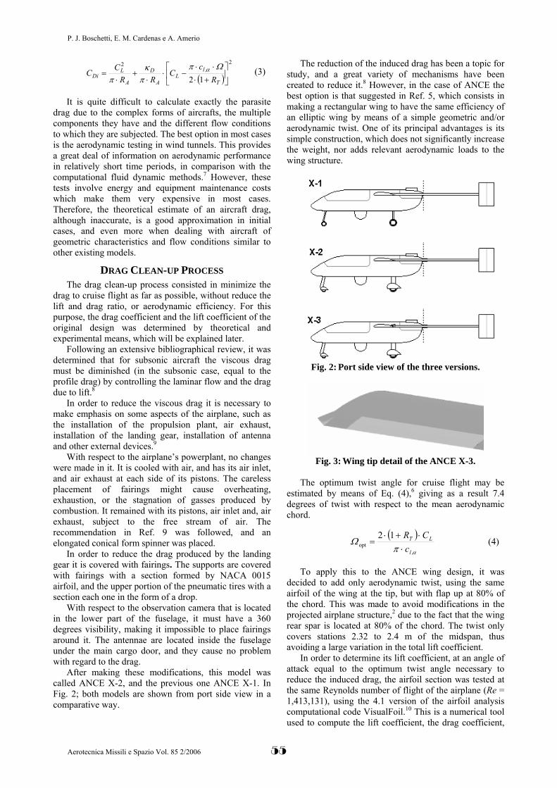
After making these modifications, this model was called ANCE X-2, and the previous one ANCE X-1. In Fig. 2; both models are shown from port side view in a comparative way.

The reduction of the induced drag has been a topic for study, and a great variety of mechanisms have been created to reduce it.8 However, in the case of ANCE the best option is that suggested in Ref. 5, which consists in making a rectangular wing to have the same efficiency of an elliptic wing by means of a simple geometric and/or aerodynamic twist. One of its principal advantages is its simple construction, which does not significantly increase the weight, nor adds relevant aerodynamic loads to the wing structure.

Fig. 2: Port side view of the three versions.

Fig. 3: Wing tip detail of the ANCE X-3.

The optimum twist angle for cruise flight may be

estimated by means of Eq. (4),6 giving as a result 7.4 degrees of twist with respect to the mean aerodynamic chord.

( )

απΩ

,l

LT

cCR

⋅⋅+⋅

=12

opt (4)

To apply this to the ANCE wing design, it was decided to add only aerodynamic twist, using the same airfoil of the wing at the tip, but with flap up at 80% of the chord. This was made to avoid modifications in the projected airplane structure,2 due to the fact that the wing rear spar is located at 80% of the chord. The twist only covers stations 2.32 to 2.4 m of the midspan, thus avoiding a large variation in the total lift coefficient.

In order to determine its lift coefficient, at an angle of attack equal to the optimum twist angle necessary to reduce the induced drag, the airfoil section was tested at the same Reynolds number of flight of the airplane (Re = 1,413,131), using the 4.1 version of the airfoil analysis computational code VisualFoil.10 This is a numerical tool used to compute the lift coefficient, the drag coefficient,



and the moment coefficient for NACA airfoil sections of four and five digits, and its analysis is based on the vortex panel method for an ideal incompressible flow.

Then the airfoil with flap at 80% of the chord was tested, until determining one that had the same lift coefficient as that resulting for the simple profile at Ωopt. The resulting flap deflection is 14 degrees upwards.

The modified design with the modified wing tips, beside the modifications of ANCE X-2, was called X-3, and Fig. 2 shows in port side view, in comparison with the other variations. Figure 3 shows the wing tip three-dimensional detail. Both design modifications were evaluated using theoretical and experimental ways.

THEORETICAL ESTIMATION OF THE AERODYNAMIC DRAG

In order to make an appropriate theoretical calculation of the aerodynamic drag, it is necessary to analyze its causes. All the components of the airplane generate drag when tested separately, and the sum of these, plus the drag caused by the interaction between components is the total drag.

In the case of the airplane under study, it may be said that the drag produced by the fuselage, the wing, the horizontal and vertical stabilizers, plus the drag produced by secondary components, such as those of the landing gear, the observation camera, and the engine radiator, and the drag produced by interaction, generate the total drag of the airplane. The factors involved in the estimation of the drag coefficient of the airplane may be observed in Eq. (5).

(5) intDDcsDvDhDwDfD CCCCCCC +++++=

The fuselage drag coefficient is calculated using Eq. (6), which is an approximation of experimental results realized at high Reynolds numbers.11,12

⎥⎥

⎦

⎤

⎢⎢

⎣

⎡

⎟⎟⎠

⎞⎜⎜⎝

⎛⋅+⋅+⋅⋅=

2

2154300030f

f

f

f

f

fDf l

dld

.dl

.C (6)

In the particular case where the fuselage is not of circular section, the frontal diameter average of the fuselage is equal to 2π-1/2Af2

1/2. The reference area of the calculated coefficient is the frontal area, which is the reason why the drag coefficient obtained must be multiplied by the expression 4-1 π df

2 Sw-1 to be used in the

Eq. (5). The drag coefficient of the wing corresponds to Eq.

(7); this is only valid when the airplane is on level flight where the lift generated by the vertical and horizontal stabilizers is insignificant, and all the induced drag is produced by the wing.

(7) DiDpwDw CCC +=

The profile drag coefficient of the wing and other surfaces, such as the horizontal and vertical stabilizers, produced when the lift from these is zero, is estimated by adding the pressure drag coefficient produced by friction

on the surface and the pressure drag coefficient produced by the airfoil, as may be seen on Eq. (8).11

( ) ( ) ⎥⎦⎤

⎢⎣⎡ ⋅+⋅+⋅=

4602212 c

tc

t.CC fDpw (8)

The estimated friction coefficient is equal to 1.33/Re0.5 for laminar regime,13 and 0.455/(log10 Re)2.58 for the turbulent regime.14

The drag due to interaction is the result of the mutual interaction between the boundary layer of a surface and that of the body in contact with this surface. According to previous studies, the drag produced by two adhered bodies is far greater than the drag of these two bodies separately, inclusive from 30 to 55% of the smaller body drag.13 The interaction drag is supposed to be a function of the thickness of the boundary layer on the contact walls and may be estimated for the joints between walls and airfoil sections by means of the reference areas of the mentioned surfaces, and the maximum thickness and chord of the airfoil section, as shown in Eq. (9).11,12

( ) ( )( ) 21

2

22100030750

AAt

ct.ct.A,AC intD +

⋅⎥⎥⎦

⎤

⎢⎢⎣

⎡−= (9)

In the calculation of the interaction drag coefficient are involved, as may be seen from Eq. (10), the drag coefficients due to interaction wing – fuselage, horizontal stabilizer – vertical stabilizers, and secondary components – fuselage. The first two cases may be calculated by means of Eq. (9), because it involves airfoils sections and walls, but in the case of secondary components, which consists of the adherence of bodies it is convenient to follow the recommendation of Ref. 13, and suppose that it is 30% higher than the drag coefficient of each secondary component.

( ) ( ) csintDvhintDfwintDintD CS,SCA,SCC ++= 1 (10)

However, according to previous experimental studies,15 the induced drag between walls and airfoils, such as the one existing between the wing and the fuselage, varies depending on the relative vertical position of the wing with respect to the fuselage.

THEORETICAL AND NUMERICAL ESTIMATION OF LIFT COEFFICIENT

For this investigation, the lift coefficient estimate was made by means of the Prandtl’s Lift Line Theory,16 which is quite effective for calculating the lift distribution and lift coefficient in rectangular wings with no swept or dihedral.

For this purpose a numerical code was created and programmed to obtain the lift coefficient at different angles of attack, and at different Reynolds numbers. In the program, the solution for the equation for the spanwise lift distribution is obtained using a Fourier’s series, based on the method developed by Glauert and Lotz,17 and the total lift coefficient is calculated by simple integration. The program is capable of printing the lift coefficient, the lift line slope, and to plot the lift



distribution curve knowing only the wingspan, the root chord, the tip chord, the geometric and aerodynamic twist, the airfoil section lift slope of each station for a determined Reynolds number, and the number of spanwise stations.

DimeSurfa

Wing Medium

LengThe slope of the lift curve is obtained by means of the

ratio cl/a, using data obtained through a computer code for airfoil analysis, VisualFoil,10 at Reynolds flight number from 18 to -15 degrees with respect to the mean aerodynamic chord.

Fi

WIND – TUNNEL TESTING Following the theoretical study of the lift coefficients

and drag coefficient of each design modification it is necessary to carry out aerodynamic tests in the wind tunnel.

The experiments were carried out between December 2003 and March 2005, using only one wind tunnel, model Rollab SWT – 009, located within the facilities of the aeronautical engineering laboratory of the UNEFA, in Maracay, Venezuela. The wind tunnel is a closed – circuit, closed throat, and unpressurized facility. It has a square test section of 0.32 m × 0.32 m with transparent walls, and it was specially designed to test wings and small three-dimensional models at low speeds.

The normal testing range is for airflow speed from 14 to 47 m/s, and it is determined by means of the pressure differences between the test section and the downwash section. The wind tunnel has a three component TEM balance capable of measuring lift, drag and moment.

The model support mechanism is capable of an angle of attack from 40 to -40 degrees, although these may vary depending on the support being used. The models are fastened from below the test section on three struts. Depending on the type of the model to be tested, it is usual to use extensions on these supports in order to avoid the least interference between the supports and the model.

For the present study, a calibration of the tunnel was carried out before each run, in order to guarantee the accuracy of the scale, the aerodynamic alignment angle, and the turbulence factor, which resulted in 1.38.

For this purpose a rectangular wing of 0.254 m span and 0.052 m of chord, formed by NACA 0015 airfoil section was used. The symmetric characteristic of the airfoil section facilitates the obtainment of the aerodynamic alignment angle.

The wing was tested in each run from 16 to -16 degrees, at different velocities in order to obtain lectures at different Reynolds number values. After due considerations to the fact that this was a straight wing,18 the obtained results were compared with those presented in the literature,19,20 showing discrepancies with the stall region values reported in Ref. 20, but not with those reported in Ref. 19.

Based on the blueprints for model ANCE X-1, a fiberglass, reinforced with polyester resin wind tunnel model was constructed, and painted in black. The test section size limited the scale, permitting a maximum wingspan of 0.256 m, which gave a scale of 1:20.2 for the models to be tested. The airfoil section used on the wing of the model is NACA 4415, and the one used for the tail

surface isThe seconANCE Xmaterials gear and dimensioncomparedand 5 shANCE X-

Each position, speeds innumbers. correctioncomplete

TheoreticBefore

coefficiencalculatioFor modewing on mdeflectionaerodynam



Table 1: Reference dimensions nsion Full scale 1 to 20.2 scale ce, m2 2.899 0.007105 span, m 5.18 0.256 chord, m 0.604 0.030 th, m 4.65 0.231

g. 4: ANCE X-1 wind tunnel model.

Fig. 5: ANCE X-2 wind tunnel model.

NACA 0009 section, according to the design. d scale model, based on the blueprints of model -2, was made with the same moulds and as scale test model X-1, to which in the landing spinner modifications were incorporated. The s of the two models are shown in table 1, being with those of the full scale airplane. Figures 4 ow photographs of the wind tunnel models 1 and X-2, respectively. model was tested held in an upside down at different angles of attack and at several order to obtain data at different Reynolds Buoyancy, blockage, and tare-and-interferences s were applied. See Ref. 21 for a more discussion of methods and process.

RESULTS AND DISCUSSION al Analysis and Numerical Simulation begin the theoretical calculations of the drag t generated by ANCEs X-1, X-2, and X-3, the n of the wing lift coefficient was carried out. ls X-1 and X-2 the wing is identical, while the

odel X-3 has a small variation at the tip. The at the wing tip was made applying ic twist between stations 2.32 and 2.4

(measured in meters) of the midspan, and for this it was necessary to altered the original program code. In the case of the untwisted wing a data convergence of 10-6 was achieved, while for the twisted wing was about 10-4, using a one hundred and one stations in both cases. The input parameters are shown in table 2 and the results in table 3. Having the lift coefficient of the two proposed wings, it was possible to calculate the induced drag coefficient at each angle of attack using Eq. (3).

Then the drag coefficient of each aircraft component was estimated using Eqs. (6) to (10), and the total drag coefficient by using Eq. (5). The results corresponding to the three models are shown on table 4, for cruise flight condition, and the drag polar of the three models is plotted in Fig. 6. In this, the efficiency increase of model X-3 with respect to model X-2 and of the latter with respect to X-1 can be appreciated. The global drag coefficient variation, from model X-1 with respect to model X-3, is significant. The results show a drag decrease of 4.24% with respect to X-2, and of 7.38% with

respect to X-3. The landing gear modifications generated 57.39% of the drag coefficient variation, and the 42.61% to the decrease of the induced drag.

Table 2: Input data parameters to the code Wing Geometry X-1 and X-2 X-3

Effective wing span, m 4.8 4.8 Tip chord, m 0.604 0.604

Root chord, m 0.604 0.604 Angle of attack, deg 6.37 6.37

Twisted, deg 0 7.4 Airfoil Flow Conditions

Lift section Airfoil NACA 4415 Reynolds number 1413131

Compressible effects No Transition on laminar separation

Wind Tunnel Testing Based on all results obtained in the wing tunnel tests,

the values of the uncertainties related with the final results were calculated. For this purpose the possible variables that may interfere in final results were analyzed. The airflow temperature, pressure differences, lift and drag variations were taken into consideration. The standard deviation for lift coefficient estimated is ±0.0027, for drag coefficient ±0.0003, and for the airflow speed ±0.04 m/s.

Table 3: Data obtained of wing lift coefficient at different angles of attack

CLwα, deg X-1, X-2 X-3

16 1.1095 1.1021 14 1.4252 1.4167 12 1.5359 1.5269 10 1.4384 1.4293 8 1.3246 1.3154 6 1.1403 1.131 4 0.9954 0.9861 2 0.8035 0.7941 0 0.6115 0.6021 -2 0.4195 0.4101 -4 0.2275 0.2181 -6 0.0355 0.0262 -8 -0.156 -0.166

The results obtained for the X-1 design tested model are summarized in Fig. 7-9. Figures 7, 8, and 9 show the lift coefficient, and the drag coefficient, both as a function of angle of attack, and the polar curve for each Reynolds number obtained, respectively.

Figures 10, and 11 show the lift coefficient, and the drag coefficient as a function of angle of attack, obtained at different Reynolds numbers for the ANCE X-2 wind tunnel model. Figure 12 shows the lift and drag ratio of the same model.

Figures 13 and 14 show the lift coefficient curves as a function of Reynolds number for several angles of attack of the models ANCE X-1 and X-2 respectively. For all the angles of attack these curves present a depression Rew between 8.4×104 and 8.7×104, and they have a similar behavior. For some major angles of attack the lift coefficient presents a negative slope at the end of the curve.

Fig. 6: Theoretical approach of polar curves for each ANCE model.

Table 4: Summary of data obtained for drag theoretical analysis CDcs

CDpw

CDh +

CDv

CDf CDint Camera Powerplant Landing gear

CDpCDi

(α=0) CD

X-1 0.0113 0.0036 0.0004 0.0039 0.0037 0.0042 0.0037 0.0308 0.0160 0.0468 X-2 0.0113 0.0036 0.0004 0.0033 0.0037 0.0042 0.0023 0.0288 0.0160 0.0448 X-3 0.0113 0.0036 0.0004 0.0033 0.0037 0.0042 0.0023 0.0288 0.0145 0.0433 ∆CD 0 0 0 -0.0006 0 0 -0.0014 -0.0020 -0.0015 -0.0035



Fig. 7: Lift coefficient as a function of angle of attack of ANCE X-1 wind tunnel model.

Fig. 10: Lift coefficient as a function of angle of

attack of ANCE X-2 wind tunnel model.

Fig. 8: Drag coefficient as a function of angle of attack of ANCE X-1 wind tunnel model.

Fig. 11: Drag coefficient as a function of angle of

attack of ANCE X-2 wind tunnel model.

Fig. 9: Polar curve of ANCE X-1 wind tunnel model, at several Reynolds Numbers.

Fig. 12: Polar curve of ANCE X-2 wind tunnel

model, at several Reynolds Numbers.



Fig. 13: Lift coefficient as a function of Reynolds

Number of ANCE X-1 wind tunnel model.

Fig. 15: Drag coefficient as a function of Reynolds


Fig. 14: Lift coefficient as a function of Reynolds

Number of ANCE X-2 wind tunnel model. Fig. 16: Drag coefficient as a function of Reynolds


Figures 15 and 16 show the drag coefficient curves as a function of Reynolds number for several angles of attack. In these, a trend similar to rounded bodies can be observed, the curves fall progressively until reaching their lowest points at Ref between 4.2×105 and 4.4×105, a slight increase and, finally, a slight negative slope. This represents the transition from laminar to turbulent flow condition, very usual in Reynold numbers similar to those studied. At low angles of attack the lifting surfaces produce low lift values. At high angles of attack the slopes following the depressions tend to be more pronounced than those observed at angles of attack close to zero.

Scale Effects Conversion Due to the fact that the tests were not carried out at

the flight Reynolds number, it is necessary to apply the scale effects correction. For this purpose the data obtained at the wind tunnel for both test models, at the highest Reynolds number, were used. With these the procedure described in Ref. 21 for the correction of scale

effects over the drag coefficient (extrapolation method), and over the lift coefficient curve (Jacob´s method) was carried out.

In order to correct the scale effects over the lift coefficient curve the results of Ref. 19 were considered, where the slope of the lift curve of the NACA 4415 airfoil section is different for Reynolds numbers similar to those of these study with respect to those of flight. In the curves shown in Fig. 9 and 12 the zero lift angle approximately coincides with those shown in Ref. 19 together with the slope of the lift curve which would result for a finite rectangular wing.20 Although Ref. 19 does not offer details of the behavior of this airfoil for such low Reynolds numbers. It may be observed that for Re higher than 8.3×104, the slope of the lift curve is equal to the corresponding 1.26×106, only for low lift coefficients. In order to extrapolate the lift coefficient curve, the slope of the lift curve corresponding to the ANCE X-2 model data, for Rew equal to 1.2×105, with lift coefficients under 0.3 were taken. The maximum lift coefficient and the stall data were taken from the data



Fig. 17: Drag coefficient as a function of angle of

attack for ANCEs X-1, X-2, and X-3.

Fig. 18: Lift coefficient of ANCEs X-1, X-2, and X-

3, as a function of angle of attack.

obtained through the numerical simulation of the wing. The same lift coefficient curve was taken for ANCE X-1, due to both have the same configuration, and the ANCE X-1 does not have data at these angles of attack.

Fig. 19: Polar curves of ANCEs X-1, X-2, and X-3.

The data obtained from the wind tunnel tests with ANCE X-2 scale test model were used for determine the features of the X-3 version. The only difference between both versions is the wing tip twist, which does not affect the slope of the lift curve, as revealed by the numerical study which was carried out. However, there is a lift coefficient variation between the original wing and the twisted wing equal to 0.0094. Thus, in order to determine the lift curve of the ANCE X-3 in flight, the same slope of the lift curve of the X-2 version was taken, and each CL obtained was diminished in 0.0094. The maximum lift coefficient and the stall data were taken from the numerical study.

The drag coefficient curve of the ANCE X-3 was plotted by means of a variation on the extrapolation method, adding the parasite drag coefficient of the wing tunnel model ANCE X-2, to the induced drag coefficient calculated with the X-3 model lift coefficient.

Figures 17 and 18 show the lift coefficient and the drag coefficient as a function of angle of attack for ANCEs X-1, X-2, and X-3. Figure 19 shows the polar curve of the three versions of the design. From this, the increase of optimum efficiency and the cruise flight efficiency of the X-3 model with respect to X-2, and the drag with respect to the X-1, can be appreciated. Note the landing gear modification only help to minimize the drag at low angles of attack, and the wing tip modification reduce the drag near to the cruise lift coefficient and high angles of attack.

Table 5 shows the comparison of the drag coefficient obtained with the wind tunnel testing data for cruise flight. These results reveal that the improvement applied in the landing gear yield a ∆CD of -0.0028 (73.7% of ∆CD), and the twists applied to the wing a ∆CD of -0.001 (26.1% of ∆CD). Between both the total drag coefficient variation is of -0.0038. This means a decrease in the drag coefficient of 7.98% with respect to the initial one. Table

5 also shows the aerodynamic efficiency for each version of the ANCE. ANCE X-2 resulted to be 5.88% more efficient than X-1, and ANCE X-3, 6.49%.

CONCLUSION A detailed theoretical analysis of aerodynamic

resistance, a wide range of wind tunnel tests on scale models, and a numerical code based on Prandtl’s Lift Line Theory, were fundamental tools in the ANCE aerodynamic drag cleanup process. The modifications made on the landing gear, and the variation in local wing tip twist resulted in an efficiency increase when applied to the ANCE design. These modifications produced a total efficiency increase of 6.03% when estimated by the theoretical method, and 6.49% based on experiment results, and a drag decrease of 0.0035 theoretically calculated, and of 0.0038 experimentally obtained.

Although the theoretical analysis is a good start for this type of studies, and its results show the approximate performance of an aircraft in flight, this is not reliable due to the difference between the theoretical calculated data,



6. Phillips, W. F., Fugal, S. R. and Spall, R., “Minimizing Induced Drag with Geometric and Aerodynamic Twist, CFD Validation,” AIAA Paper 2005-1034, Jan. 2005.

7. Miller, C. G., "Development of X-33/X-34 Aerothermodynamic Data Bases: Lessons Learned and Future Enhancements," NATO-AVT Symposium, Paper RTO-MP-35, Oct. 1999.

8. Bushnell, B. M., “Aircraft Drag Reduction – a review,” Journal of Aerospace Engineer, Vol. 217, No 1, 2003, pp. 1-18.

9. Coe, P., “Review of Drag Cleanup Test in Langley Full – Scale Tunnel (from 1935 to 1945) Applicable to Current General Aviation Airplanes,” NASA TN D-8206, Jun. 1976.

Table 5: Drag coefficient at cruise flight condition for the three versions of ANCE

X-1 X-2 X-3 CD 0.0476 0.0448 0.0438 ∆CD - -0.0028 -0.0038

CL/CD 12.406 13.181 13.268

and the experimental data, obtained from wind tunnel testing.

10. Visual Foil/Model Foil, Ver. 4.1, Hanley Innovations, Ocala, FL, 2001.

11. Hoerner, S. F. Résistance á L’avancement dans les Fluides, edited by Gauthier Villars Editeurs, Paris, France, 1965, Chapter XIV.

The aerodynamic data generated at UNEFA facilities has been used to feed the database for the ANCE vehicle. This database will be used to estimate the performance, and flight capacities of the airplane.

12. Zeidan, F., “Estudio Teórico-Practico de la Resistencia al Avance de una Aeronave,” Aerodinámica y Práctica Avanzada, edited by Consejo de Publicaciones de la Universidad de los Andes, Mérida, Venezuela, 1995, pp. 89-96. ACKNOWLEDGMENTS 13. Von Mises, R., “Air Resistance or Parasite Drag,” Theory of Flight, edited by Dover Publications, Inc., New York, 1959, pp. 95-111.

The authors wish to thanks the financial support of Direction of Investigation, Universidad Simón Bolívar, Caracas, and FUNDACITE Aragua, Maracay, both in Venezuela. We also want to acknowledge to the Department of Aeronautical Engineering of Universidad Nacional Experimental Politécnica de la Fuerza Armada, Maracay, for allowing the use of the aerodynamic laboratory facilities.

14. Rebuffet, P., “Phénomènes el principes généraux,” Aérodynamique Expérimentale, Tome 1, edited by Librairie Polytechnique Béranger, Paris, France, 1966, pp. 102.

15. Prandtl, L., “Effects of Varying the Relative Vertical Position of Wing and Fuselage,” NACA TN-75, 1921.

16. Prandtl, L., “Applications of Modern Hydrodynamics to the Aeronautics,” NACA TR-116, 1921.

17. Peery, D. J., “Spanwise Air-Load Distribution,” Aircraft Structures, edited by McGraw Hill Book Company, New York, 1950, pp. 213-249. REFERENCES

18. Anderson, J. D., “Incompressible Flow over Finite Wings”, Fundamentals of Aerodynamics, 2nd ed., McGraw-Hill, Inc., New York, 2002, pp. 340-347.

1. Boschetti, P. J., and Cárdenas, E. M., “Diseño de un Avión No Tripulado de Conservación Ecológica,” Theses, Department of Aeronautical Engineering, Universidad Nacional Experimental Politécnica de la Fuerza Armada, Maracay, Venezuela, 2003. 19. Jacobs, E. N., and Sherman, A., “Airfoil Section Characteristics

as Affected by Variations of the Reynolds Number,” NACA R-586, 1937.

2. Cárdenas, E. M., Boschetti, P. J., Amerio, A., and Velásquez, C. D., “Design of an Unmanned Aerial Vehicle for Ecological Conservation,” AIAA Paper 2005-7056, Sep. 2005. 20. Sheldahl, R. and Klimas, P., “Aerodynamic Characteristics of

Seven Symmetrical Airfoil Sections Through 180-Degree Angle of Attack for use in Aerodynamic Analysis of Vertical Axis Wind Turbines,” Sandia National Laboratories, Albuquerque, NM, SAND80-2114, Mar. 1981.

3. Lausetti, A., “La Polare del Velivolo,” Esercizi di Mecánica del Volo, edited by Libreria Editrice Universitaria Levrotto & Belle, Torino, Italy, 1975. pp. 10-17.

4. Vennard, J. and Street, R., “Fluid Flow about Immersed Objects,” Elementary Fluid Mechanics, 5th ed., edited by John Wiley & Son, Inc., New York, 1976, pp. 645-692.

5. Phillips, W. F., “Lifting-Line Analysis for Twisted Wings and Washout-Optimized Wings,” AIAA Journal of Aircraft, Vol. 41, No. 1, 2004, pp. 128-136.

21. Rae, W. H., and Pope, A., Low-Speed Wind Tunnel Testing, 2nd ed, edited by Wiley Interscince Publication, New York, 1984, pp. 198-205, 419-424, 457-464.



drag clean-up process of the unmanned...

Documents