draft - securities litigation & consulting group volatility smiles...draft crooked volatility...

DRAFT

Crooked Volatility Smiles: Evidence from Leveraged andInverse ETF Options

Geng Deng, PhD, CFA, FRM∗ Tim Dulaney, PhD, FRM†

Craig McCann, PhD, CFA‡ Mike Yan, PhD, FRM§

January 7, 2014

AbstractWe find that leverage in exchange traded funds (ETFs) can affect the “crookedness” of

volatility smiles. This observation is consistent with the intuition that return shocks areinversely correlated with volatility shocks – resulting in more expensive out-of-the-moneyput options and less expensive out-of-the-money call options. We show that the prices ofoptions on leveraged and inverse ETFs can be used to better calibrate models of stochasticvolatility. In particular, we study a sextet of leveraged and inverse ETFs based on the S&P500 index. We show that the Heston model (Heston , 1993) can reproduce the crooked smilesobserved in the market price of options on leveraged and inverse leveraged ETFs. We showfurther that the model predicts a leverage dependent moneyness, consistent with empiricaldata, at which options on positively and negatively leveraged ETFs have the same price.Finally, by analyzing the asymptotic behavior for the implied variances at extreme strikes,we observe an approximate symmetry between pairs of LETF smiles empirically consistentwith the predictions of the Heston model.

1 Introduction

1.1 Empirical Motivation

By relating option prices to observables (such as strike prices, time-to-expiration, spot price, etc.)and one unknown parameter (implied volatility of the underlying asset return dynamics), Black

∗Director of Research, Office: (703) 890-0741, Email: [email protected].†Senior Financial Economist, Office: (703) 539-6777, Email: [email protected].‡President, Office: (703) 539-6760, Email: [email protected].§Senior Financial Economist, Office: (703) 539-6780, Email: [email protected].

1

DRAFT

Preliminary draft, please do not quote or distribute

and Scholes (1973) allowed practitioners to more systematically study observed option prices. Fur-thermore, this unknown parameter allowed researchers to normalize comparisons between optionswith different observables.

For all of the success of the Black-Scholes model and for its near-ubiquity today, there areseveral shortcomings of the model. For example, Rubinstein (1985) pointed out strike price biasesand close-to-maturity biases by studying the prices of the most active option on the CBOE.1 Insubsequent works, Rubinstein (1994) and Jackwerth and Rubinstein (1996) showed that optionson stocks and stock options exhibit volatility skew and that foreign currency options exhibit avolatility smile (at-the-money options are cheaper than in-the-money or out-of-the-money options).

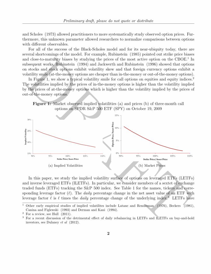
In Figure 1, we show a typical volatility smile for call options on equities and equity indices.2

The volatilities implied by the prices of in-the-money options is higher than the volatility impliedby the prices of at-the-money options which is higher than the volatility implied by the prices ofout-of-the-money options.

Figure 1: Market observed implied volatilities (a) and prices (b) of three-month calloptions on SPDR S&P 500 ETF (SPY) on October 19, 2009

15%

20%

25%

30%

90% 95% 100% 105% 110%

Imp

lied

Vo

lati

lity

Strike Price/Asset Price

(a) Implied Volatilities

0%

5%

10%

15%

90% 95% 100% 105% 110%

Op

toin

Prc

e/

Ass

et

Pri

ce


(b) Market Prices

In this paper, we study the implied volatility surface of options on leveraged ETFs (LETFs)and inverse leveraged ETFs (ILETFs). In particular, we consider members of a sextet of exchangetraded funds (ETFs) tracking the S&P 500 index. See Table 1 for the names, tickers and corre-sponding leverage factor (`). The daily percentage change in the net asset value of an ETF withleverage factor ` is ` times the daily percentage change of the underlying index.3 LETFs have

1 Other early empirical studies of implied volatilites include Latane and Rendleman (1976), Beckers (1981),Canina and Figlewski (1993) and Derman and Kani (1994).

2 For a review, see Hull (2011).3 For a recent discussion of the detrimental effect of daily rebalancing in LETFs and ILETFs on buy-and-hold

investors, see Dulaney et al (2012).

2

DRAFT


Table 1: Sextet of LETFs tracking the S&P 500 index

Fund Name Ticker `ProShares UltraPro Short S&P 500 ETF SPXU -3ProShares UltraShort S&P 500 ETF SDS -2ProShares Short S&P 500 ETF SH -1SPDR S&P 500 ETF SPY 1ProShares Ultra S&P 500 ETF SSO 2ProShares UltraPro S&P 500 ETF UPRO 3

leverage factor ` ≥ 1 while ILETFs have leverage factor ` ≤ −1.4

According to the Black-Scholes model, an option on an LETF with leverage factor ` ≥ 1 shouldhave the same price as an option on an ILETF with leverage factor (−`) if both options sharethe same strike price and expiration – if these ETFs share the same underlying index.5 This isintuitive because, in risk-neutral valuation, the only difference between the evolution of the LETFor ILETF is the leverage factor that proportionally increases the volatility. Since the option priceis dependent upon the square of the volatility, the price of options on LETFs and ILETFs withthe same strike and expiration should have the same price.

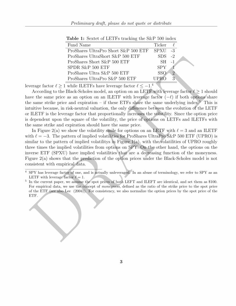
In Figure 2(a) we show the volatility smile for options on an LETF with ` = 3 and an ILETFwith ` = −3. The pattern of implied volatilities for ProShares UltraPro S&P 500 ETF (UPRO) issimilar to the pattern of implied volatilitys in Figure 1(a), with the volatilities of UPRO roughlythree times the implied volatilities from options on SPY. On the other hand, the options on theinverse ETF (SPXU) have implied volatilities that are a decreasing function of the moneyness.Figure 2(a) shows that the prediction of the option prices under the Black-Scholes model is notconsistent with empirical data.

4 SPY has leverage factor of one, and is actually unleveraged. In an abuse of terminology, we refer to SPY as anLETF with leverage factor ` = 1.

5 In the current paper, we assume the spot prices of both LEFT and ILEFT are identical, and set them as $100.For empirical data, we use the concept of moneyness, defined as the ratio of the strike price to the spot priceof the ETF (see also Lee (2004)). For consistency, we also normalize the option prices by the spot price of theETF.

3

DRAFT


Figure 2: Market observed implied volatilities (a) and prices (b) of three-month calloptions on ProShares UltraPro Short S&P 500 ETF (SPXU) and ProShares UltraPro

S&P 500 ETF (UPRO) for different strike prices on October 19, 2009

45%

60%

75%

90%

75% 95% 115% 135% 155% 175%

Imp

lied

Vo

lati

lity


SPXU (l = -3) UPRO (l = 3)

(a) Implied Volatilities

0%

5%

10%

15%

20%

25%

30%

75% 95% 115% 135% 155% 175%

Op

tio

n P

rice/

Ass

et

Pri

ce


SPXU (l = -3) UPRO (l = 3)

(b) Market Prices

Figure 2(b) shows the price of call options on these leveraged ETFs as a function of thenormalized strike price. These observations suggest that the crookedness of the volatility smile isdependent on the leverage factor `.

The prices of in-the-money call options on positively leveraged ETFs (`1 ≥ 1) imply lowervolatilities than the prices of in-the-money call options on ILETFs (`2 ≤ 0) for the same levelof leverage (`1 = |`2|) and moneyness. Similarly, the prices of out-of-the-money call options onpositively leveraged ETFs imply lower volatilities than the prices of out-of-the-money call optionson ILETFs for the same level of leverage and moneyness.6

Intuitively, we expect stock returns to be negatively correlated with volatility shocks – e.g.large price decline and an increase in volatility. As a result, far from the money put options aremore expensive than one may naively expect. As a result, the volatility implied by option marketprices are increasing with decreasing moneyness, as shown in Figure 2(a). For an inverse ETF,stock returns would be positively correlated with volatility shocks – e.g. large price declines inthe underlying leads to large price increases in the inverse ETF. As a result, the volatility impliedby option market prices on inverse ETFs should be increasing with increasing moneyness. Thecombination of these two arguments implies that low moneyness options on positively leveragedETFs will be more expensive than similar options on negatively leveraged ETFs.

We explore this phenomenon, as well as the crossing phenomena shown in Figure 2(b), bothempirically and theoretically in this paper.7 Although this phenomenon is intuitive, there has been

6 Both of these statements make the implicit assumption that the prices are being compared on options with thesame moneyness and maturity.

7 The strike price at which the prices of call options on LETFs and ILETFs are equal is another common featureof the options data.

4

DRAFT


no study of the crossing behavior depicted in Figure 2(b) and this paper seeks to fill this gap.

1.2 Observable Implications

We use the stochastic volatility model in Heston (1993) to explain the “crooked smiles” in theoptions market. This Heston model, similar to the Black-Scholes model, has closed-form solutionsfor the valuation of European put and call options but incorporates stochastic volatility.

Unlike the constant implied volatility in the Black-Scholes model, the dynamics of the volatilityis correlated with the dynamics of the stock price or index level in the Heston model. Thisstochastic volatility model is better equipped to account for observed skewness and kurtosis ofreturn distributions.8

Volatility smiles have often been explained either by jump-diffusion models as suggested byMerton (1976) or with stochastic volatility as in models proposed by Hull and White (1987) andHeston (1993). We consider the Heston model here because of the convenient analytic properties.

Option pricing in the context of leveraged ETFs has recently gained interest in the literature.Ahn et al (2012) and Zhang (2010) use standard transformation methods to price options onETFs and LETFs within the Heston stochastic volatility framework. We extended their researchby deriving the dynamics of LETFs. The closed-form solutions use a Green function approachfollowing the method in Lipton (2001). Our numerical simulations show that the Heston modelcan explain the patterns in option prices on LETFs and ILETFs. We observe that the crookedsmile is present only when there exists non-zero correlation between the Brownian motions for theasset returns and the variance.9 Furthermore, we show that the model predicts a moneyness –dependent upon the level of leverage – for which the prices of positively and negatively leveragedETF options have the same price and that this prediction is consistent with empirical data.

We also study the asymptotic behavior of implied variance curves for options on LETF andILETF. This analysis relies heavily upon the moment expansion framework in Lee (2004) andRollin et al (2009). Subsequently analyses – (Friz et al , 2011) and (de Marco and Martini ,2012) – refined the volatility smile expansion within the Heston model. Building upon Lee’s work,Benaim and Friz (2009) showed how the tail asymptotics of risk-neutral returns can be directlyrelated to the asymptotics of the volatility smile and they applied this approach to time-changedLevy models and the Heston model (Benaim and Friz (2008)).

We provide empirical evidence that the asymptotic slopes of the implied variance curves foroptions on LETF and ILETF show an approximate symmetry and that this approximate symmetryis consistent with the Heston model. In particular, we show that the large-strike asymptotic slopes

8 Derman and Kani (1994) discuss the connection between the dynamics of the underlying stock price – whichdetermines the moments of the return distribution – and the volatility smile. The Heston model has been studiedbefore as an explanation for volatility smiles present in the Black-Scholes model – see, for example, Sircar andPapanicolaou (1999).

9 When the correlation is zero, the Heston model is equivalent to the Black-Scholes model.

5

DRAFT


of the implied variance curves for LETFs are related to the small-strike asymptotic slopes of theimplied variance curves for ILETFs. Both simulated examples and market data are presented.

The rest of the paper is organized as following. In Section 2, we review the Black-Scholes model,and Heston stochastic volatility model. The closed-form solution of the call options of LETF andILETF is derived under Heston dynamics. In Section 3, the asymptotic behaviors of the optionprices are studied as the moneyness goes extremely large and small. In Section 4, we simulate theoption prices under Heston dynamics, and compare the prices across different leverage numbers `.In addition, we calibrate our model using the empirical data in Section 5. The paper is concludedin Section 6.

2 Leveraged and Inverse ETF Option Prices

2.1 The Black-Scholes Model

If an asset price St follows a geometric Brownian motion, then its dynamics are described by theclassic stochastic differential equation

dStSt

= (µ− q)dt+ σdWt,

where µ, q, and σ are expected return, dividend yield and implied volatility of the asset, respec-tively. All three parameters are assumed to be constant and continuously compounded. The priceof an LETF or ILETF Lt, which tracks ` times daily return of the underlying asset, satisfies

dLtLt

= (µ` − q`)dt+ σ`dWt.

where µ` = `µ and σ` = `σ. This implies that the volatilities of the returns are leveraged |`| times.Under risk-neutral assumptions, the expected return of the LETFs µl is the risk-free rate

r, independent of l. Therefore, the option price C(t, L), satisfies the following Black-Scholesequation:10

∂C

∂t+

1

2σ2`2L2∂

2C

∂L2+ (r − q`)L

∂C

∂L− rC = 0, (1)

where r is the constant risk-free rate.In this model, the volatility (the standard deviation for the instantaneous ETF return dLt/Lt)

is always |`|σ, and is independent of the strike price of the option contract, as well as the sign of theleverage number `. If both LETF and ILETF have the same leverage factor in absolute value andthe same dividend yield q`, we should observe the same implied volatility and same option priceunder the Black-Scholes model. Figure 2(b) shows that this theoretical prediction is inconsistentwith observed market option prices.

10 For simplicity, we drop the subscript t for the price process Lt.

6

DRAFT


2.2 Heston’s Stochastic Volatility Model

Since the Black-Scholes model is not able to adequately describe the phenomena observed in theoption prices on the sextet of leveraged ETFs in Section 2.1, we turn to alternative models of assetdynamics. We choose to discuss the Heston model (Heston , 1993) in particular because of theclosed-form solutions for European option prices and the depth of literature analyzing the detailsof the model.

In the risk-neutral framework, we write Lt as the price of the LETF or ILETF, vt as thevariance of the underlying stock. These variables are governed by the dynamics

dLtLt

= (r − q`)dt+ `√vtdW1t; (2)

dvt = κ(θ − vt)dt+ ε√vtdW2t. (3)

where W1t and W2t are two Brownian motions with a correlation value ρ, i.e.,

E [dW1tdW2t] = ρdt. (4)

A simple derivation shows the stochastic process Lt is linked to the underlying stock priceprocess St and the realized variance

∫ t0vtdt

LtL0

=

(StS0

)lexp

(l − l2

2

∫ t

0

vsds+ (1− l)r). (5)

The equation implies that a higher realized variance implies a larger deviation between the holdingperiod returns of LETFs and those of the underlying stock. Though the equation cannot be directlyused in valuing options on LETFs, it shows the necessity of using stochastic volatility models sincedynamic variance is an important component of the return of LETFs.11

Utilizing the following theorem, we derive the call option value for LETFs.

Theorem 1. The value of an European call option with strike K for an LETF in the Heston modelis in the form

C(Lt, v0, τ) = KeXt2−rτU(τ,Xt, v0), (6)

where v0 is the initial variance value at time 0 and τ is the time to maturity τ = T − t. Xt isdefined as ln Ft

K, where Ft is the forward price of LETF and is defined as Ft = Lte

(r−q)τ . Thefunction U(τ,Xt, v0) is given by Equation (19) in Appendix A.

Proof. See proof in Appendix A.

11 For a constant volatility model, the realized variance is simply∫ t

0vdt = vt. For a more complete discussion of

this topic, see (Avellaneda and Zhang , 2010).

7

DRAFT


Alternatively, a single set of change variables could simplify the valuation approach. If weintroduce the following change of variables12

vt = `2vt;

θ = `2θ;

ε = |`|ε; (7)

ρ = Sign(`)ρ;

The stochastic differential equations in Equation (2) and Equation (3) are converted into thefollowing standard Heston model

dLtLt

= (r − q)dt+√vtdW1t; (8)

dvt = κ(θ − vt)dt+ ε√vtdW2t. (9)

Note that the new equations are free of the leverage factor ` thus we can use the Lipton solutionor Heston solution given ` = 1. Having derived the dynamics of leveraged and inverse ETFs basedupon the dynamics of the underlying index, we move on to consider the pricing of options onleveraged and inverse ETFs.

3 Symmetry in Implied Variances for LETF Options

In this section, we study the implications of Andersen and Piterbarg (2007) to the extreme strikebehavior of option prices on leveraged and inverse ETFs.13 Our results build heavily upon thework by Lee (2004) wherein the author showed that the extreme strike behavior is related to thenumber of finite moments of the return distribution.14

In particular, at large strikes the Black-Scholes implied variance becomes a linear function ofthe logarithm of the strike price. Lee (2004) showed that the small strike asymptotic behavior isalso a linear function of the logarithm of the strike price using the properties of the inverse priceprocess.

Following Friz and Keller-Ressel (2009), a model is said to exhibit moment explosion at orderα > 1 if there exists some finite T ∗(α) such that E [SαT ∗ ] = ∞. The time of moment explosion,T ∗(α) depends on the moment under consideration and is the smallest time such that E [Sαt ] <∞.

If, for some β, E[Sβt

]is finite for all t, then T ∗(β) =∞.

12 This change of variables is consistent with that given by Proposition 1 in Ahn et al (2012).13 Andersen and Piterbarg (2007) have studied the time of moment explosion within the Heston model.14 See Leung and Sircar (2012) for a recent study of implied volatility surfaces implied by the market prices of

options on LETFs.

8

DRAFT


Lee (2004) showed that the large strike (K � F0) Black-Scholes implied variance is related tothe degree of moment explosion through the following theorem.15

Theorem 2. If p∗ = sup{p | E

[S1+pT

]<∞

}and βR = lim supx→∞

σ2BS(x)

|x|/T , then

βR = 2− 4(√

p∗(p∗ + 1)− p∗). (10)

Lee (2004) showed further that the extreme small strike (K � F0) asymptotic behavior of theBlack-Scholes implied volatility can be related to the degree of moment explosion of the inverseprice process through the following theorem.

Theorem 3. If q∗ = sup{q | E

[S−qT

]<∞

}and βL = lim supx→∞

σ2BS(x)

|x|/T , then

βL = 2− 4(√

q∗(q∗ + 1)− q∗). (11)

When βL or βR are zero, the underlying model does not exhibit moment explosion. Note thatp∗ = α∗+ − 1, where α∗+ is the degree of moment explosion, or the critical moment for the processSt at time T and q∗ = α∗−, where α∗− is the critical moment for the inverse price process S−1T attime T .

Andersen and Piterbarg (2007), in their Proposition 3.1, show how to relate the degree ofmoment explosion α+ to the parameters in the Heston model as well as the time of momentexplosion T ∗(α+). Following Corollary 6.2 in Andersen and Piterbarg (2007), the critical momentα∗+ is obtained by solving T ∗(α+) = T .

To solve the critical moment α∗− for the inverse price process, Rollin (2008) showed that if anasset follows a price process described by the Heston model, then the inverse spot price follows aprice process described by the Heston model with the following parameters

κ = κ− ρε, ρ = −ρ and θ = κθ/κ (12)

where the parameters {κ, θ} represent the analogous parameters in the inverse spot price processto those in the non-inverted price process. Using these results, we can study the symmetry ofBlack-Scholes implied variances at extreme strikes for options on LETFs and ILETFs.

Referring to the parameter translations in Equation (7), we see that the LETF price processLt,` is closely linked to the inverse of the ILETF price process Lt,−` Lt,` ≈ L−1t,−`. The followingtable shows the corresponding parameters used for the two price processes when we combine theresults in Equation (7) with the result in Equation (12).

15 Here we use the notation x = log(K/F0) for the moneyness with respect to the stock’s forward price for contractsexpiring T years from today.

9

DRAFT


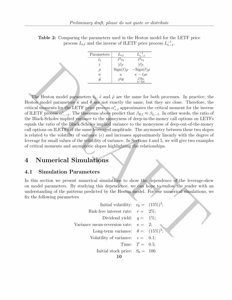
Table 2: Comparing the parameters used in the Heston model for the LETF priceprocess Lt,` and the inverse of ILETF price process L−1t,−`.

Parameters Lt,` L−1t,−`vt `2vt `2vtε |`|ε |`|ερ Sign(`)ρ −Sign(`)ρκ κ κ− `ρεθ `2θ `2θκ

κ−`ρε

The Heston model parameters vt, ε and ρ are the same for both processes. In practice, theHeston model parameters κ and θ are not exactly the same, but they are close. Therefore, thecritical moments for the LETF price process α∗+,l approximates the critical moment for the inverseof ILETF process α∗−,−l. The theorems above predict that βR,` ≈ βL,−`. In other words, the ratio ofthe Black-Scholes implied variance to the moneyness of deep-in-the-money call options on LETFsequals the ratio of the Black-Scholes implied variance to the moneyness of deep-out-of-the-moneycall options on ILETFs of the same leveraged amplitude. The asymmetry between these two slopesis related to the volatility of variance (ε) and increases approximately linearly with the degree ofleverage for small values of the volatility of variance. In Sections 4 and 5, we will give two examplesof critical moments and asymptotic slopes highlighting the relationships.

4 Numerical Simulations

4.1 Simulation Parameters

In this section we present numerical simulations to show the dependence of the leverage-skewon model parameters. By studying this dependence, we can hope to endow the reader with anunderstanding of the patterns predicted by the Heston model. For our numerical simulations, wefix the following parameters

Initial volatility: v0 = (15%)2;

Risk-free interest rate: r = 2%;

Dividend yield: q = 1%;

Variance mean-reversion rate: κ = 2;

Long-term variance: θ = (15%)2;

Volatility of variance: ε = 0.1;

Time: T = 0.5;

Initial stock price: S0 = 100.10

DRAFT


In what follows, we vary the correlation ρ between returns and return variance, the leveragenumber `, and the strike price K (or equivalently, the moneyness). By varying these parameters,we analyze the model and explain the pattern implied by market prices of options on leveragedand inverse ETFs. The model calibration on the empirical data will be discussed in Section 5.

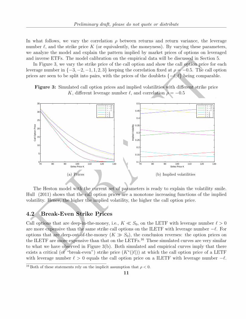
In Figure 3, we vary the strike price of the call option and show the call option price for eachleverage number in {−3,−2,−1, 1, 2, 3} keeping the correlation fixed at ρ = −0.5. The call optionprices are seen to be split into pairs, with the prices of the doublets {−`, `} being comparable.

Figure 3: Simulated call option prices and implied volatilities with different strike priceK, different leverage number `, and correlation ρ = −0.5

70 80 90 100 110 120 1300

5

10

15

20

25

30

35

Strike Price K

Cal

l Opt

ion

Pric

e

ℓ = −3ℓ = −2ℓ = −1ℓ = 1ℓ = 2ℓ = 3

(a) Prices

70 80 90 100 110 120 1300.1

0.15

0.2

0.25

0.3

0.35

0.4

0.45

0.5

Strike Price K

Impl

ied

Vol

atili

ty

ℓ = −3ℓ = −2ℓ = −1ℓ = 1ℓ = 2ℓ = 3

(b) Implied volatilities

The Heston model with the current set of parameters is ready to explain the volatility smile.Hull (2011) shows that the call option prices are a monotone increasing functions of the impliedvolatility. Hence, the higher the implied volatility, the higher the call option price.

4.2 Break-Even Strike Prices

Call options that are deep-in-the-money, i.e., K � S0, on the LETF with leverage number ` > 0are more expensive than the same strike call options on the ILETF with leverage number −`. Foroptions that are deep-out-of-the-money (K � S0), the conclusion reverses: the option prices onthe ILETF are more expensive than that on the LETFs.16 These simulated curves are very similarto what we have observed in Figure 3(b). Both simulated and empirical curves imply that thereexists a critical (or “break-even”) strike price (K∗(|`|)) at which the call option price of a LETFwith leverage number ` > 0 equals the call option price on a ILETF with leverage number −`.16 Both of these statements rely on the implicit assumption that ρ < 0.

11

DRAFT


Table 3 reports those critical strike prices that results in equality between the prices of optionson LETFs and ILETFs within the same doublet (` = ±|`|) for our numerical simulations. Inthis particular set of parameters, the break-even strike price/moneyness decreases as the leveragefactor increases.

Table 3: Summary of the break-even strike prices that lead to the same option valuesfor leveraged ETFs within the same doublet (` = ±|`|). For these simulations, we use

ρ = −0.5

Leverage Number K∗(|`|) Option Price` = ±1 $99.944 $4.459` = ±2 $98.289 $9.414` = ±3 $95.592 $14.794

Table 3 demonstrates the dependence of the break-even prices on the leverage |`|. In Figure4, we plot the difference between call option prices on the LETF and ILETF within the samedoublet for different values of the correlation coefficient ρ. This set of graphs shows that the pricedifference of the call options is symmetric with respect to ρ. The simulations further show thatthe break-even strike prices, when the option price differences equal zero, are independent of ρ.

12

DRAFT


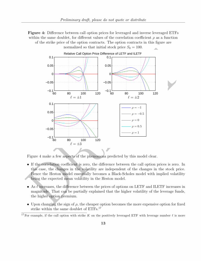
Figure 4: Difference between call option prices for leveraged and inverse leveraged ETFswithin the same doublet, for different values of the correlation coefficient ρ as a function

of the strike price of the option contracts. The option contracts in this figure arenormalized so that initial stock price S0 = 100.

60 80 100 120−0.1

−0.05

0

0.05

0.1

ℓ = ±160 80 100 120

−0.1

−0.05

0

0.05

0.1

ℓ = ±2

60 80 100 120−0.1

−0.05

0

0.05

0.1

ℓ = ±3

ρ = −1

ρ = −0.5

ρ = 0

ρ = 0.5

ρ = 1

Relative Call Option Price Difference of LETF and ILETF

Figure 4 make a few aspects of the phenomena predicted by this model clear.

• If the correlation coefficient is zero, the difference between the call option prices is zero. Inthis case, the changes in the volatility are independent of the changes in the stock price.Hence the Heston model essentially becomes a Black-Scholes model with implied volatilitybeing the expected mean volatility in the Heston model.

• As ` increases, the difference between the prices of options on LETF and ILETF increases inmagnitude. That can be partially explained that the higher volatility of the leverage funds,the higher option premium.

• Upon changing the sign of ρ, the cheaper option becomes the more expensive option for fixedstrike within the same doublet of ETFs.17

17 For example, if the call option with strike K on the positively leveraged ETF with leverage number ` is more

13

DRAFT


• The break-even strike price within each doublet is independent of ρ. Although we presentonly a handful of correlation examples in Figure 4, this conclusion holds for all values of ρ.

Note that deep-out-of-the-money call options on ILETFs are more expensive than deep-out-of-the-money call options on LETFs when ρ < 0. If the correlation coefficient ρ is negative, thevolatility and the price of ILETF tend to increase simultaneously. With the same parameters, theprice of LETF increases, while the volatility tends to decrease. Intuitively, the ILETF option hasa higher probability of ending in-the-money than the analogous LETF. As a result, the call optionprices on an ILETF with high strike are often more expensive than call option prices on an LETFwhen stock price and implied volatility are negatively correlated.

4.3 Asymptotic Implied Variance Slope

We explore the correspondence present between high-strike asymptotic behavior of positively lever-aged ETFs and low-strike asymptotic behavior of negatively leveraged ETFs in Table 4. In thiscontext, it is conventional to study implied variance – as opposed to implied volatility – since im-plied variance has an asymptotically linear relationship to the logarithm of the strike price whileimplied volatility has a non-linear asymototic relationship.

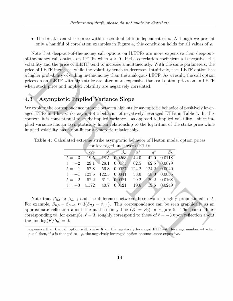
Table 4: Calculated extreme strike asymptotic behavior of Heston model option pricesfor leveraged and inverse ETFs

α∗+ p∗ βR α∗− q∗ βL` = −3 19.5 18.5 0.0263 42.0 42.0 0.0118` = −2 29.1 28.1 0.0175 62.5 62.5 0.0079` = −1 57.8 56.8 0.0087 124.2 124.2 0.0040` = +1 123.5 122.5 0.0041 58.0 58.0 0.0085` = +2 62.2 61.2 0.0081 29.2 29.2 0.0168` = +3 41.72 40.7 0.0121 19.6 19.6 0.0249

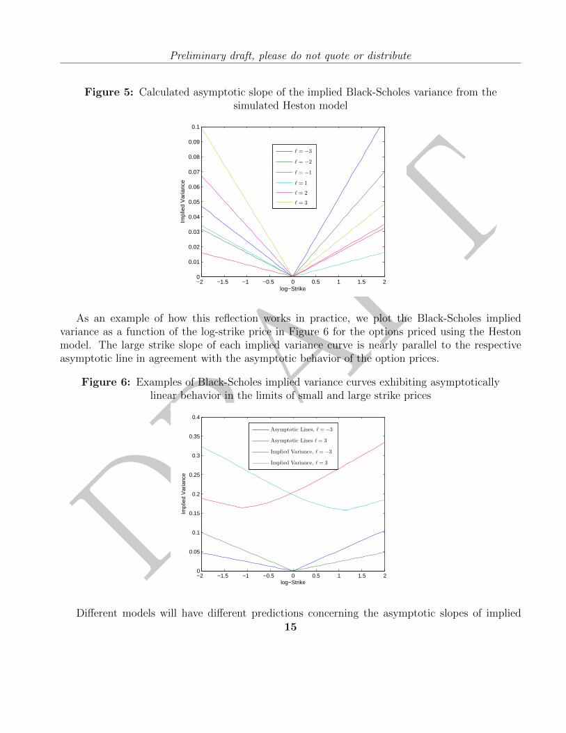
Note that βR,` ≈ βL,−` and the difference between these two is roughly proportional to `.For example, βR,3 − βL,−3 ≈ 3(βR,1 − βL,1). This correspondence can be seen graphically as anapproximate reflection about the at-the-money line (K = S0) in Figure 5. The pair of linescorresponding to, for example, ` = 3, roughly correspond to those of ` = −3 upon reflection aboutthe line log(K/S0) = 0.

expensive than the call option with strike K on the negatively leveraged ETF with leverage number −` whenρ > 0 then, if ρ is changed to −ρ, the negatively leveraged option becomes more expensive.

14

DRAFT


Figure 5: Calculated asymptotic slope of the implied Black-Scholes variance from thesimulated Heston model

−2 −1.5 −1 −0.5 0 0.5 1 1.5 20

0.01

0.02

0.03

0.04

0.05

0.06

0.07

0.08

0.09

0.1

log−Strike

Impl

ied

Var

ianc

e

ℓ = −3

ℓ = −2

ℓ = −1

ℓ = 1

ℓ = 2

ℓ = 3

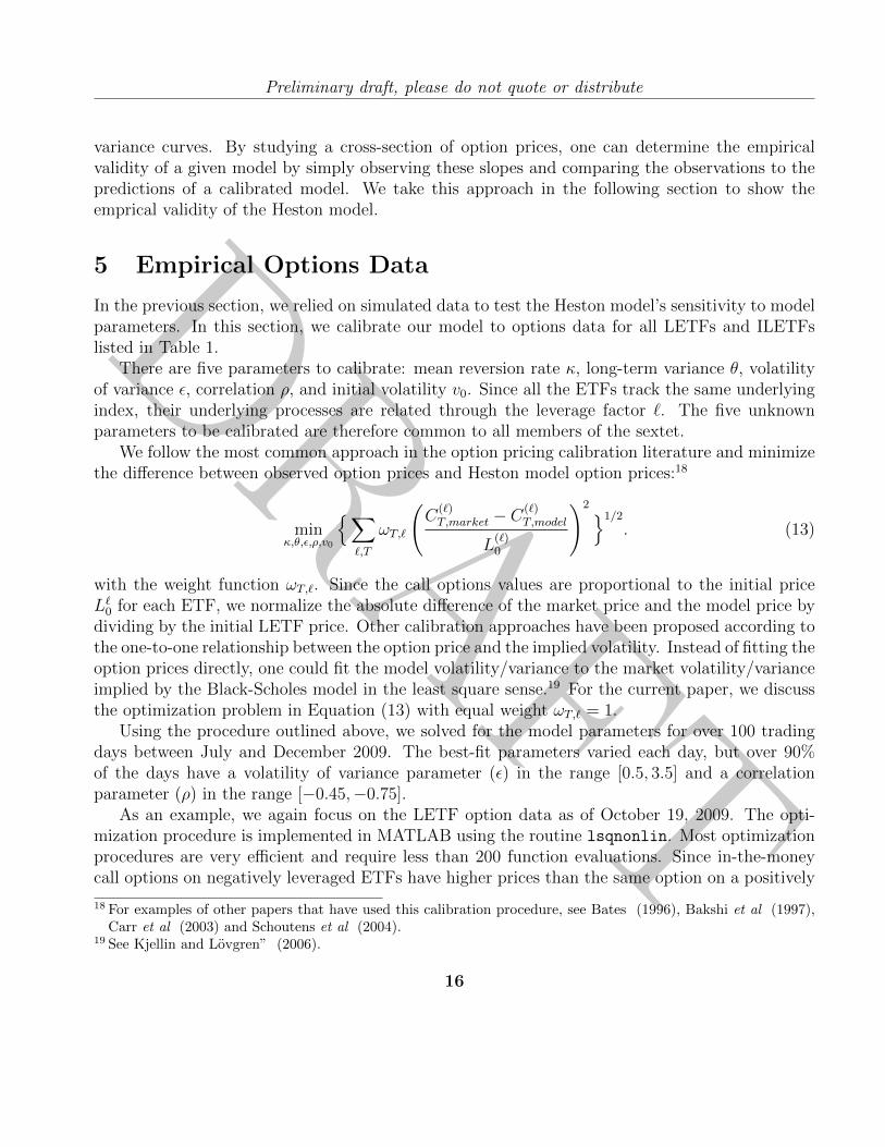
As an example of how this reflection works in practice, we plot the Black-Scholes impliedvariance as a function of the log-strike price in Figure 6 for the options priced using the Hestonmodel. The large strike slope of each implied variance curve is nearly parallel to the respectiveasymptotic line in agreement with the asymptotic behavior of the option prices.

Figure 6: Examples of Black-Scholes implied variance curves exhibiting asymptoticallylinear behavior in the limits of small and large strike prices

−2 −1.5 −1 −0.5 0 0.5 1 1.5 20

0.05

0.1

0.15

0.2

0.25

0.3

0.35

0.4

log−Strike

Impl

ied

Var

ianc

e

Asymptotic Lines, ℓ = −3

Asymptotic Lines ℓ = 3

Implied Variance, ℓ = −3

Implied Variance, ℓ = 3

Different models will have different predictions concerning the asymptotic slopes of implied15

DRAFT


variance curves. By studying a cross-section of option prices, one can determine the empiricalvalidity of a given model by simply observing these slopes and comparing the observations to thepredictions of a calibrated model. We take this approach in the following section to show theemprical validity of the Heston model.

5 Empirical Options Data

In the previous section, we relied on simulated data to test the Heston model’s sensitivity to modelparameters. In this section, we calibrate our model to options data for all LETFs and ILETFslisted in Table 1.

There are five parameters to calibrate: mean reversion rate κ, long-term variance θ, volatilityof variance ε, correlation ρ, and initial volatility v0. Since all the ETFs track the same underlyingindex, their underlying processes are related through the leverage factor `. The five unknownparameters to be calibrated are therefore common to all members of the sextet.

We follow the most common approach in the option pricing calibration literature and minimizethe difference between observed option prices and Heston model option prices:18

minκ,θ,ε,ρ,v0

{∑`,T

ωT,`

(C

(`)T,market − C

(`)T,model

L(`)0

)2 }1/2

. (13)

with the weight function ωT,`. Since the call options values are proportional to the initial priceL`0 for each ETF, we normalize the absolute difference of the market price and the model price bydividing by the initial LETF price. Other calibration approaches have been proposed according tothe one-to-one relationship between the option price and the implied volatility. Instead of fitting theoption prices directly, one could fit the model volatility/variance to the market volatility/varianceimplied by the Black-Scholes model in the least square sense.19 For the current paper, we discussthe optimization problem in Equation (13) with equal weight ωT,` = 1.

Using the procedure outlined above, we solved for the model parameters for over 100 tradingdays between July and December 2009. The best-fit parameters varied each day, but over 90%of the days have a volatility of variance parameter (ε) in the range [0.5, 3.5] and a correlationparameter (ρ) in the range [−0.45,−0.75].

As an example, we again focus on the LETF option data as of October 19, 2009. The opti-mization procedure is implemented in MATLAB using the routine lsqnonlin. Most optimizationprocedures are very efficient and require less than 200 function evaluations. Since in-the-moneycall options on negatively leveraged ETFs have higher prices than the same option on a positively

18 For examples of other papers that have used this calibration procedure, see Bates (1996), Bakshi et al (1997),Carr et al (2003) and Schoutens et al (2004).

19 See Kjellin and Lovgren” (2006).

16

DRAFT


Table 5: Heston model calibration using market prices of options on the sextet ofleveraged and inverse leveraged ETFs

κ θ ε ρ v06.8791 0.0669 1.3357 -0.5649 0.0359

leveraged ETFs, we expect the correlation between the asset price and variance to be negative.Indeed, our results indicate the best fit value for the correlation is −0.565.

Since our model uses more options data (option data over a sextet of LETFs), the calibratedparameters are more precisely determined and stable when compared to a calibration using onlyoptions on the unleveraged member of the sextet (SPY, ` = 1).

Given the calibrated model parameters in Table 5, we can compute the asymptotic behaviorof the implied variance curves. The results of this computation are summarized in Table 6.

Table 6: Calculated extreme strike asymptotic behavior of Heston model aftercalibration to market prices of options on the sextet of ETFs with the S&P 500 as the

underlying index on October 19, 2009

α∗+ p∗ βR α∗− q∗ βL` = −3 3.510 2.510 0.1672 9.246 9.246 0.0513` = −2 5.055 4.055 0.1101 13.348 13.348 0.0361` = −1 9.710 8.710 0.0543 25.679 25.679 0.0191` = +1 24.711 23.711 0.0207 9.973 9.973 0.0478` = +2 12.862 11.862 0.0405 5.185 5.185 0.0881` = +3 8.919 7.919 0.0594 3.597 3.597 0.1225

The difference between β(`)R and β

(−`)L is more pronounced here than in Table 4 as a result of

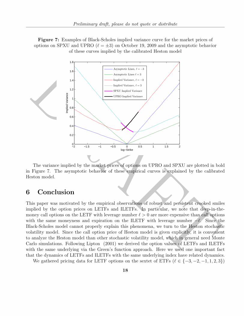
the volatility of variance ε. This calibrated parameter ε is more than ten times larger than thatused for the numerical simulations in Section 4. We plot the implied variance curves of the marketprices as well as the asymptotic implied variance lines in Figure 7 for SPXU (` = −3) and UPRO(` = +3).

17

DRAFT


Figure 7: Examples of Black-Scholes implied variance curve for the market prices ofoptions on SPXU and UPRO (` = ±3) on October 19, 2009 and the asymptotic behavior

of these curves implied by the calibrated Heston model

−2 −1.5 −1 −0.5 0 0.5 1 1.5 20

0.2

0.4

0.6

0.8

1

1.2

1.4

1.6

1.8

log−Strike

Impl

ied

Var

ianc

e

Asymptotic Lines, ℓ = −3

Asymptotic Lines ℓ = 3

Implied Variance, ℓ = −3

Implied Variance, ℓ = 3

SPXU Implied Variance

UPRO Implied Variance

The variance implied by the market prices of options on UPRO and SPXU are plotted in boldin Figure 7. The asymptotic behavior of these empirical curves is explained by the calibratedHeston model.

6 Conclusion

This paper was motivated by the empirical observations of robust and persistent crooked smilesimplied by the option prices on LETFs and ILETFs. In particular, we note that deep-in-the-money call options on the LETF with leverage number ` > 0 are more expensive than call optionswith the same moneyness and expiration on the ILETF with leverage number −`. Since theBlack-Scholes model cannot properly explain this phenomena, we turn to the Heston stochasticvolatility model. Since the call option price of Heston model is given explicitly, it is convenientto analyze the Heston model than other stochastic volatility model, which in general need MonteCarlo simulations. Following Lipton (2001) we derived the option values of LETFs and ILETFswith the same underlying via the Green’s function approach. Here we used one important factthat the dynamics of LETFs and ILETFs with the same underlying index have related dynamics.

We gathered pricing data for LETF options on the sextet of ETFs (` ∈ {−3,−2,−1, 1, 2, 3})

18

DRAFT


with the S&P 500 as the underlying index. We showed that the Heston model can reproducethe crooked smiles observed in the empirical data and, using numerical simulations, showed howdifferent phenomena in the options data could be produced with different model parameters.In particular, we studied the asymptotic behavior of Black-Scholes implied volatility curves andcompared these to the predictions given by the Heston model calibrated to the market prices ofoptions.

An important contribution of this paper is that using options data of LETFs and ILETFs inaddition to options data on the underlying index itself can better calibrate the pricing dynamicsof the index. Using the closed-form solutions for the option prices of LETFs and ILETFs derivedin this paper, practitioners can more effectively and accurately determine the model parameters.

A Appendix

Proof of theorem 1 We follow Lipton (2001) for modeling and solving the call option priceson leverage ETFs. Choosing the risk premium λ = λ0

√v we find that the option price C(L, v, τ)

follows 20

Cτ −1

2v`2L2CLL − ερv`SCLv −

1

2ε2vCvv − (r − q)LCL − κ(θ − v)Cv + rC = 0, (14)

where τ = T − t is the time-to-maturity for the option, κ is the new mean-reversion rate and θnew is mean-reversion variance level, respectively.21 To simplify the equation above, we write theequation in terms of the forward price (F ) and introduce C(τ, F, v), such that

C(τ, F, v) = erτC(τ, L, v);

F = Le(r−q)τ .

Then the new variable satisfies the

Cτ −1

2v`2F 2CFF − ερv`F CFv −

1

2ε2vCvv − κ(θ − v)Cv = 0, (15)

We can write this equation in terms of dimensionless variables by introducing

X = lnF

K= ln(

S0

K) + (r − q)τ

⇒ U(τ,X, v) = e−X/2C(τ, F, v)

K. (16)

20 Again, for simplicity, we drop the subscript t for the both Lt and vt.21 Where κθ = κθ and κ = κ+ λ0ε.

19

DRAFT


Hence U(τ,X, v) satisfies

Uτ −1

2v`2UXX − ερv`UXv −

1

2ε2vUvv − κ(θ − v)Uv +

1

8v`2U = 0. (17)

Equation (17) can be solved by introducing a Green’s function and applying the boundary conditionrelevant for the option at interest through the Spectral method (Lipton , 2001). In particular, thesolution takes the form

U(τ,X, v) =1

2π

∫ ∞−∞

∫ ∞−∞

eik(X′−X)Z(τ, k, v)U(0, X ′, v)dkdX ′. (18)

where

Z(τ, k, Y, v) = exp{ κκθε2

τ + ik`τρκθ

ε− 2κθ

ε2[ζτ + ln(

−µ+ ζ + (µ+ ζ)e−2ζτ

2ζ) + 2πiN ]

− v`2(k2 + 1/4)(1− e−2ζτ )2(−µ+ ζ + (µ+ ζ)e−2ζτ )

}(19)

µ(k) = −1

2(ik`ερ+ κ)

ζ(k) =1

2

√k2`2ε2(1− ρ2) + 2ik`ερκ+ κ2 +

ε2`2

4κ = κ− ε`ρ/2.

The boundary condition of European call options is given by the payoff at maturity

C(τ = 0, L, v) = max(L−K, 0). (20)

In terms of dimensionless variables, this boundary condition can be written as

U(0, X, v) = max(eX/2 − e−X/2, 0

). (21)

Since eX/2 is monotically increasing and e−X/2 is monotonically decreasing, it follows thateX/2 − e−X/2 ≥ 0 for all X ≥ 0. We change the order of integration in Equation (18) to evaluatethe X ′ integral first. This integral takes the simple form given by∫ ∞

0

eikX′(eX′/2 − e−X′/2

)dX ′. (22)

By Evaluating the integral, we derive

U(τ,X, v) = eX/2Z(τ, i/2, v)− 1

2π

∫ ∞−∞

e−ikXZ(τ, k, v)

k2 + 1/4dk

= eX/2Z(τ, i/2, v)− 1

π

∫ ∞0

Real(e−ikXZ(τ, k, v))

k2 + 1/4dk.

20

DRAFT


In the last step we used the fact that Z(τ,−k, v) = Z(τ, k, v).22 The value of a European calloption in the Heston model is therefore given by Equation (16).

References

Ahn, A., Haugh, M., and Jain, A. (2012) Consistent Pricing of Options on Leveraged ETFs.Working paper.

Andersen, L., and Piterbarg, V. (2007) Moment explosions in stochastic volatility models. Financeand Stochastics 11: 29-50.

Avellaneda, M., and Zhang, S. (2010) Path-Dependence of Leveraged ETF Returns. SIAM Journalon Financial Mathematics 1(1): 586-603.

Bakshi, G., Cao, C., and Chen, Z. (1997) Empirical Performance of Alternative Option PricingModels. Journal of Finance 52(5): 2003-2049.

Bates, D. (1996) Jumps and Stochastic Volatility: Exchange Rate Process Implicit in DeutscheMark Options. The Review of Financial Studies 9(1): 69-107.

Beckers, S. (1981) Standard Deviations Implied in Option Process as Predictors of Future StockPrice Variability. Journal of Banking and Finance 5: 363-382.

Benaim, S., and Friz, P. (2008) Smile Asymptotics II: Models with Known Moment GeneratingFunctions. Journal of Applied Probability 45(1): 16-32.

Benaim, S., and Friz, P. (2009) Regular Variation and Smile Asymptotics. Mathematical Fi-nance 19(1): 1-12.

Black, F., and Scholes, M. (1973) The Pricing of Options and Corporate Liabilities. Journal ofPolitical Economy 81: 637-654.

Canina, L., and Figlewski, S. (1993) The Informational Content of Implied Volatility. Review ofFinancial Studies 6: 659-681.

Carr, P., German, H., Madan, D., and Yor, M. (2003) Stochastic Volatility for Levy Process.Mathematical Finance 13: 345-382.

de Marco, S., and Martini, C. (2012) Term Structure of Implied Volatility in Symmetric Modelswith Applications to Heston. International Journal of Theoretical and Applied Finance 15(4).

22Z(τ, k, v) denotes the complex conjugation of Z(τ, k, v)

21

DRAFT


Derman, E., and Kani, I. (1994) The Volatility Smile and Its Implied Tree. RISK 2: 139-145.

Dulaney, T., Husson, T., and McCann, C. (2012) Leveraged, Inverse and Futures-Based ETFs.PIABA Bar Journal 19(1): 83-107.

Friz, P., and Keller-Ressel, M. (2009) Moment explosions in stochastic volatility models. Ency-clopedia of Quantitative Finance.

Friz, P., Gerhold, S., Golisashvili, A., and Sturm, A. (2011) On refined volatility smile expansionin the Heston model. Quantitative Finance 11(8): 1151-1164.

Heston, S. (1993) A closed-form solution for options with stochastic volatility with applicationsto bond and currency options. Review of Financial Studies 6: 327-343.

Hull, J. (2011) Options, Futures and Other Derivatives. Prentice Hall.

Hull, J., and White, A. (1987) The Pricing of Options on Assets with Stochastic Volatilities.Journal of Finance 42: 281-300.

Jackwerth, J., and Rubinstein, M. (1996) Recovering Probability Distributions from Option Prices.Journal of Finance 51: 1611-1631.

Kjellin, R., and Lovgren, G. (2006) Option Pricing Under Stochastic Volatility. Thesis, GoteborgsUniversitet, Goteborg, Sweden.

Latane, H., and Rendleman, R. (1976) Standard Deviation of Stock Price Ratios Implied in OptionPrices. Journal of Finance 31: 369-381.

Lee, R. (2004) Standard Deviation of Stock Price Ratios Implied in Option Prices. MathematicalFinance 14(3): 469-480.

Leung, T., and Sircar, R. (2012) Implied Volatility of Leveraged ETF Options. Working Paper.

Lipton, A. (2001) Mathematical Methods for Foreign Exchange: A Financial Engineer’s Approach.World Scientific.

Merton, R. (1976) Option pricing when underlying stock distributions are discontinuous. Journalof Financial Economics 3: 125-144.

Rollin, S. (2008) Spot Inversion in the Heston Model. Working Paper.

Rollin, S., Ferreiro-Castilla, A., and Utzet, F. (2009) A new look at the Heston characteristicfunction. Working Paper.

22

DRAFT


Rubinstein, M. (1985) Nonparametric Tests of Alternative Option Pricing Models Using AllReported Trades and Quotes on the 30 Most Active CBOE Option Classes from August 23,1976 to August 31, 1978. Journal of Finance 40: 455-480.

Rubinstein, M. (1994) Implied Binomial Trees. Journal of Finance 49: 771-818.

Schoutens, W., Simons, E., and Tistaert, J. (2004) A Perfect Calibration! Now What? WilmottMagazine, March: pp. 66-78.

Sircar, K., and Papanicolaou, G. (1999) Stochastic Volatility, Smile & Asymtotics. AppliedMathematical Finance 6: 107-145.

Zhang, J. (2010) Path-Dependence Properties of Leveraged Exchanged-Traded Funds: Com-pounding, Volatility and Option Pricing. PhD thesis, NYU, New York, NY.

23

draft - securities litigation & consulting group volatility smiles...draft crooked volatility...

Documents