FINAL REPORT

Identification and Evaluation of Existing Models for Estimating Environmental Pesticide Transport to Groundwater

A North American Free Trade Agreement Project

Health Canada

United States Environmental Protection Agency

October 15, 2012 Prepared by: Reuben Baris Michael Barrett, PhD Rochelle F. H. Bohaty, PhD Marietta Echeverria

Ian Kennedy, PhD Greg Malis James Wolf, PhD Dirk Young, PhD

2

ABSTRACT Estimation of pesticide concentrations in groundwater is an important consideration of the exposure assessment in the pesticide registration process. For this reason, Canada and the United States combined efforts as part of the North American Free Trade Agreement (NAFTA) to develop a harmonized groundwater modeling protocol. This effort included the development of a common conceptual groundwater modeling scenario for regulatory purposes designed to be protective of even the most vulnerable drinking water supplies. Nineteen existing modeling programs were screened as candidate programs to implement the conceptual model. Of the 19 modeling programs screened, three were selected for further evaluation, including the Pesticide Root Zone Model (PRZM), the Pesticide Emission Assessment at Regional and Local Scales (PEARL), and the Leaching Estimation and Chemistry Model – Pesticides (LEACHM). The three finalist models were evaluated for their ability to accurately simulate water flow, pesticide concentrations, and soil temperature relative to field data. All three modeling programs performed adequately and could be applied as a tool to simulate pesticide transport to groundwater. PRZM was selected as the NAFTA regulatory tool to implement the conceptual model because of ease of use and in-house expertise required for maintenance. PRZM was further evaluated by comparing simulated pesticide concentrations to targeted and non-targeted monitoring data. For the majority of chemicals tested, PRZM-predicted pesticide concentrations represented conservative upper bound estimates of exposure in groundwater when conservative input parameters (i.e., maximum application rates, annually repeated applications, half-life assumptions, or application methods) were used. Nevertheless, there are some pesticide detections in monitoring data that are not captured by PRZM model estimates. This outcome may be a result of processes such as preferential flow or macroparticle transport, which are not accounted for in the conceptual model implemented in PRZM. With site specific adjustments to the PRZM input values, estimated pesticide concentrations compare well to monitoring data (within a factor of 10). The evaluation demonstrates that PRZM is a versatile risk assessment tool that can be used both as a screening tool and as a refined site-specific tool in risk assessment.

3

CONTENTS ABSTRACT ........................................................................................................................ 2

Contents .............................................................................................................................. 3

Chapter 1: Introduction ....................................................................................................... 6

Objectives ............................................................................................................... 6

Conceptual Model ....................................................................................................... 7

Processes Included in the Conceptual Model ......................................................... 8

Water Flow.......................................................................................................... 8

Dissipation/Degradation (abiotic or biotic) and Transportation ......................... 9

Sorption ............................................................................................................... 9

Transpiration and Pesticide Interception ............................................................ 9

Management Practices ...................................................................................... 10

Report Overview ....................................................................................................... 10

References ................................................................................................................. 10

Chapter 2: Model Screening ............................................................................................. 12

Preliminary Screen .................................................................................................... 12

Summary ................................................................................................................... 14

PRZM .................................................................................................................... 15

PEARL .................................................................................................................. 15

LEACHM .............................................................................................................. 16

References ................................................................................................................. 16

Chapter 3: Finalist Model Evaluation USING Field Studies ............................................ 20

Method Overview ..................................................................................................... 20

Study Summaries .................................................................................................. 21

Study 1: Indiana - Bromide ............................................................................... 21

Study 2: North Carolina - Bromide ................................................................... 22

Study 3: North Carolina – Bromide and Oxamyl ............................................. 22

Study 4: Indiana – Bromide, Temperature and Sulfentrazone .......................... 23

Study 5: Michigan- Temperature ...................................................................... 24

Model Parameterization ........................................................................................ 24

Results and Discussion ............................................................................................. 25

Hydrology Evaluation ........................................................................................... 25

Study 1: Indiana – Bromide .............................................................................. 25

Study 2: North Carolina—Bromide .................................................................. 27

4

Study 3: North Carolina – Bromide and Oxamyl ............................................. 29

Study 4: Indiana – Bromide, Temperature, and Sulfentrazone ......................... 32

Study 5: Michigan Temperature ....................................................................... 36

Ease of Use Evaluation ..................................................................................... 38

Summary ................................................................................................................... 38

References ................................................................................................................. 38

Chapter 4: PRZM Model Evaluation USING Groundwater Monitoring Data ................. 39

Method Overview ..................................................................................................... 39

Monitoring Program Summaries ...................................................................... 40

National Water Quality Assessment (NAWQA) Program ............................... 40

Overview ....................................................................................................... 40

Use and Limitations ...................................................................................... 41

Acetochlor Registration Partnership (ARP) Midwest Corn Production Area (MwCPA) Program ....................................................................................................... 43

Overview ....................................................................................................... 43

Use and Limitations ...................................................................................... 43

National Alachlor Well-Water Survey (NAWWS) .......................................... 44

Overview ....................................................................................................... 44

Use and Limitations ...................................................................................... 44

North Carolina PGW Study .............................................................................. 44

Overview ....................................................................................................... 44

Use and Limitations ...................................................................................... 45

USDA PDP ....................................................................................................... 45

Overview ....................................................................................................... 45

Use and Limitations ...................................................................................... 45

Modeling and Monitoring Data Comparison ................................................... 46

Results and Discussion ............................................................................................. 47

National Water Quality Assessment (NAWQA) Program ............................... 47

Acetochlor Registration Partnership (ARP) Midwest Corn Production Area (MwCPA) Program ....................................................................................................... 54

National Alachlor Well-Water Survey (NAWWS) .......................................... 57

North Carolina PGW Study .............................................................................. 58

Summary ................................................................................................................... 60

Model Performance Summary .......................................................................... 60

References ................................................................................................................. 61

5

Chapter 5: Report Conclusions ......................................................................................... 64

APPENDIX A ........................................................................................................... 66

6

Chapter 1: INTRODUCTION After the passage of the Food Quality Protection Act (FQPA) of 1996, the United States Environmental Protection Agency’s (EPA) Office of Pesticide Programs (OPP) developed SCI-GROW (Screening Concentration in Groundwater) as a screening-level tool to estimate drinking water exposure concentrations from groundwater resulting from pesticide use (Barrett, 1997). Standard use of SCI-GROW in drinking water exposure assessments began circa 1997. SCI-GROW is strictly a screening-level exposure tool and does not have the capability to consider mitigating circumstances like variability in leaching potential of different soils, weather (including rainfall), cumulative yearly applications or depth to aquifer. If SCI-GROW-based assessment results indicate that pesticide concentrations in drinking water exceed the risk concern, the ability to refine the assessment is limited. In 2004, OPP’s Environmental Fate and Effects Division (EFED) initiated evaluation of advanced methods for estimating pesticide concentrations in groundwater as part of the cumulative risk assessment of carbamate pesticides (USEPA, 2005a, 2005b). Similarly in 2004, Health Canada’s Pest Management Regulatory Agency (PMRA) published information outlining an initial direction on use of modeling to estimate pesticides in groundwater (PMRA, 2004). PMRA uses the Leaching Estimation and Chemistry Model – Pesticides (LEACHM) to account for pesticide leaching (Hutson, 2003); however, because groundwater resources in Canada and the United States are similar and many modeling aspects and needs are the same, the two organizations combined efforts as part of the North American Free Trade Agreement (NAFTA) to develop a harmonized groundwater modeling protocol.

Objectives The goals of this joint effort are to improve groundwater modeling methods for estimating pesticide concentrations in the United States and Canada and to harmonize methods used by the two countries to estimate pesticide concentrations in groundwater. To accomplish these goals, the two agencies have identified two broad objectives for this project. The first objective is to identify a common computer model that can implement the conceptual model (discussed in detail below) and estimate pesticide concentrations in groundwater. The second objective is to define common procedures for determining model input parameters from soil survey data, pesticide environmental fate studies, and pesticide use information (labels and agronomic practices). This report focuses on the first of these two objectives. The second objective is provided in ATTACHMENT 1 (Model and Scenario Development for Groundwater Estimates Using PRZM) and ATTACHMENT 2 (Guidance for Selecting Input Parameters in Modeling the Environmental Fate and Transport of Pesticides to Groundwater).

7

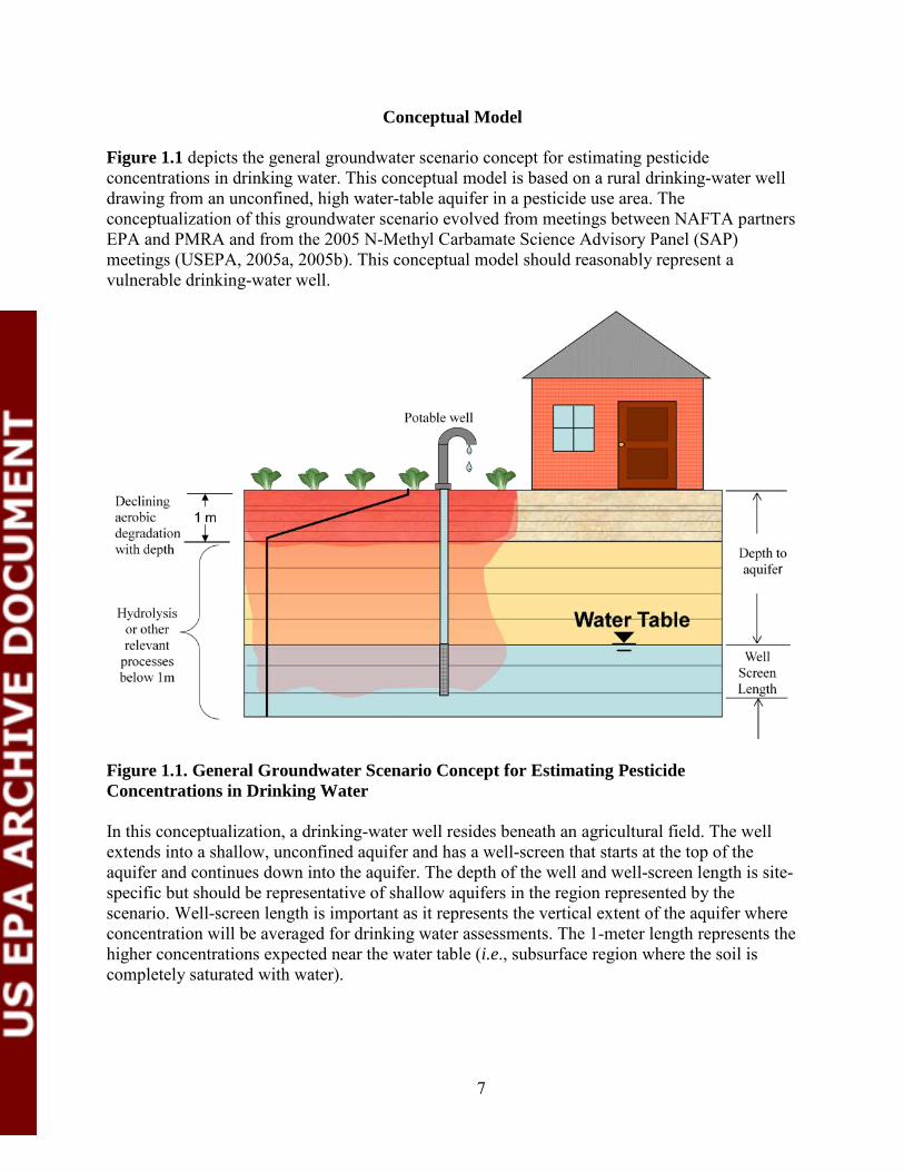
Conceptual Model Figure 1.1 depicts the general groundwater scenario concept for estimating pesticide concentrations in drinking water. This conceptual model is based on a rural drinking-water well drawing from an unconfined, high water-table aquifer in a pesticide use area. The conceptualization of this groundwater scenario evolved from meetings between NAFTA partners EPA and PMRA and from the 2005 N-Methyl Carbamate Science Advisory Panel (SAP) meetings (USEPA, 2005a, 2005b). This conceptual model should reasonably represent a vulnerable drinking-water well.

Figure 1.1. General Groundwater Scenario Concept for Estimating Pesticide Concentrations in Drinking Water

In this conceptualization, a drinking-water well resides beneath an agricultural field. The well extends into a shallow, unconfined aquifer and has a well-screen that starts at the top of the aquifer and continues down into the aquifer. The depth of the well and well-screen length is site-specific but should be representative of shallow aquifers in the region represented by the scenario. Well-screen length is important as it represents the vertical extent of the aquifer where concentration will be averaged for drinking water assessments. The 1-meter length represents the higher concentrations expected near the water table (i.e., subsurface region where the soil is completely saturated with water).

8

Processes Included in the Conceptual Model Conceptualization of pesticide transport into the aquifer includes the most important processes—those process that were likely to have the greatest impact on estimating pesticide concentrations in the aquifer—such as water flow, pesticide degradation, and sorption. Complex processes (nonlinear, non-equilibrium sorption and moisture dependent degradation) are often included in popular leaching models, but they are difficult to parameterize for a pesticide assessment given standard study data submitted as part of the pesticide registration process. This conceptualization does not preclude use of more complex processes if there is compelling evidence for use and data to support the parameterization; however, only processes that can be readily parameterized are included in the conceptual model. Complex processes such as those listed above, as well as other factors affecting pesticide degradation (e.g., moisture on plant surfaces), may be examined later if they are deemed important. The processes considered in the present conceptualization are highlighted below.

Water Flow

The conceptual model includes a water flow simulation that takes into account the effects of precipitation, evaporation, transpiration, drainage, and freezing (together with the soil temperature simulation). The moisture content in the soil profile also depends on the water flow simulation and has been reported to affect pesticide fate within the profile; however, moisture effects on pesticide fate are not included at this time due to lack of data. The application zone is considered to be a large field (e.g., a one-dimensional vertical transport model), and any localized runoff is conceptualized as eventually entering the aquifer; thus, horizontal losses (runoff) are not considered in the conceptual model. Water flows through a porous medium either as unsaturated flow (in the soil or vadose zone) or as saturated flow (in the groundwater aquifer). Two types of models are often used to represent water flow in unsaturated soils and are referred to as 1) the Richards equation and the 2) capacity or “tipping-bucket” model. Richards equation models can simulate gradual drainage and upward flow (e.g., PEARL1 and LEACHM2), while capacity models (i.e., PRZM3) simulate downward flow. Capacity models tend to run faster and require fewer parameters. The conceptual model permits the use of either of these two models for simulating water flow through the soil profile. Thus, the equation used to simulate flow will depend on the computer model selected to implement the conceptual model. Brief descriptions of these two models are provided below.

Richards Equation Model

The Richards equation describes the movement of water in unsaturated soils and was formulated by Richards (1931). It is a non-linear partial differential equation that does not have a closed-form analytical solution and needs to be solved numerically. Computers models require more run time to complete such calculations.

1 Pesticide Emission Assessment at Regional and Local Scales (Leistra et al., 2001; Tiktak et al., 2001) 2 Leaching Estimation and Chemistry Model (Hutson, 2003) 3 Pesticide Root Zone Model (Suárez, 2005)

9

Capacity or “Tipping-Bucket” Model

Water movement in a capacity model is a simpler conceptualization. When precipitation occurs the water is distributed from the top layer downward in a “tipping bucket” manner. Each layer (or bucket) fills from its initial water content to field capacity. Then the remaining or excess water is passed down to the next layer (or flows over to the next bucket) unless it is removed by evapotranspiration.

Dissipation/Degradation (abiotic or biotic) and Transportation

The conceptual model considers pesticide degradation in the soil profile. Degradation is assumed to occur faster in the top of the profile and decrease with soil depth. In addition, degradation is assumed to decrease as the temperature decreases. As with several other degradation-depth conceptualizations, this conceptual model has degradation decreasing in a linear fashion through the top one meter of the soil profile. No aerobic metabolic transformation is assumed to occur below one meter. The conceptual model, however, does not preclude alternative degradation schemes when there is compelling evidence that a pesticide behaves differently than the standard conceptualization at depths below one meter. Because temperature has important effects on degradation, soil temperature is simulated. Soil temperatures vary with season and depth and may be quite different from surface temperatures or the laboratory experimental temperature used for degradation experiments. Temperature variations should be captured both in the vertical profile or the soil as well as temporally on a seasonal basis at least. Change in abiotic and biotic degradation rates due to temperature flux can be simulated using a number of different approaches, including Q10 or Arrhenius approaches.

Sorption

Compounds moving through the soil profile can be slowed due to sorption onto soil particles or diffusion into soil organic matter. The basic conceptual model allows for linear instantaneous sorption, which would be defined by a distribution coefficient, Kd, defined as the ratio of the sorbed concentration (mass pesticide/mass soil) to soil solution concentration. For many pesticides, sorption occurs on the soil organic matter, so for cases where Kd correlates with the soil organic matter content, a Koc can be used instead.

Transpiration and Pesticide Interception

In the conceptual model, crops influence transpiration as well as pesticide interception; whereas the degradation of pesticides on foliage or the uptake of pesticides into the plant is not specifically included in the conceptual model because there is usually not enough information available to parameterize a model to include such processes. If, however, such data are available, the conceptual model can be modified to incorporate these dissipation pathways. In its current form, the conceptual model includes crop descriptions only to determine the impact on hydrology and pesticide transport, as opposed to crop productivity, degradation of pesticide on foliage, or uptake of pesticide by plants. A description of canopy coverage and root depth is sufficient to capture the most relevant plant influences on pesticide transport in the conceptual model.

10

Management Practices

The model includes some management practices that affect pesticide transport and can be readily parameterized. These include irrigation, pesticide application timing, and depth of soil incorporation. Irrigation provides significant amounts of water in some areas and may be a transport driver in some cases. Pesticide application timing information is typically available and likely will be important with respect to the weather or irrigation timing. A range of soil incorporation depths are generally known for specific applications methods, or a soil incorporation depth may be specified on the label. Simulation of other management practices such as soil manipulation, tile drainage, and pesticide application methods may be desirable but are not considered in the present conceptualization. Such processes may be considered in subsequent versions, if suitable data are available.

Report Overview The remaining chapters of this report highlight the selection of a suitable computer model for implementation of the groundwater conceptual model presented in this chapter and the evaluation of the implemented conceptual model in the selected computer model. Chapter 2 presents the full list of potential models screened for development of the conceptual model and describes the processes used to identify the most appropriate models for further evaluation. Chapter 3 presents the evaluation of the three finalist models and presents the rationale for selecting one model for implementation for regulatory purposes. Further evaluation comparing the identified computer model with monitoring data is provided in Chapter 4. This includes comparison of model output values [estimated drinking water concentration (EDWCs)] to targeted and non-targeted monitoring data.

References Barrett, M. Initial Tier Screening of Pesticides for Groundwater Concentration Using the SCI-GROW Model; U.S. Environmental Protection Agency: Washington, DC, 1997. Buckingham, E. Studies on the Movement of Soil Moisture; Bulletin 38; U.S. Department of Agriculture Bureau of Soil: Washington, DC, 1907. Hutson, J. L. Leaching Estimation and Chemistry Model (LEACHM): Model Description and User’s Guide. Flinders University of South Australia, School of Chemistry, Physics, and Earth Sciences: Adelaide, SA, 2003, 142 pp Leistra, M.; van der Linden, A.M.A.; Boesten, J.J.T.I.; Tiktak, A.; van den Berg, F. PEARL model for pesticide behavior and emissions in soil-plant systems. Description of Processes. FOCUS PEARL Version 1.1.1. Bilthoven, National Institute of Public Health and Environment. Wageningen, Alterra, Green World Research, RIVM report 71140009/Alterra- Report 013 Alterra, Wageningen, the Netherlands, 2001,107 pp. Richards, L.A., Capillary Conduction of Liquids Through Porous Mediums. J. Appl. Phys. (Physics 1) 1931, 1, 318- 333.

11

Suárez, L.A. 2005. PRZM-3, A Model for Predicting Pesticide and Nitrogen Fate in the Crop Root and Unsaturated Soil Zones: Users Manual for Release 3.12; EPA/600/R-05/111; U.S. Environmental Protection Agency, National Exposure Research Laboratory, Ecosystems Research Division: Athens, GA, 2005. 426 pp. Tiktak, A.; van den Berg, F.; Boesten, J.J.T.I; van Kraalingen, D; Leistra, M.; van der Linden, A.M.A. Manual of FOCUS PEARL Version 1.1.1; RIVM Report 711401008, Alterra Report 28; Alterra Green World Research, Wageningen, National Institute of Public Health and the Environment Bilthoven, Wageningen, The Netherlands, 2000, 144 pp. U.S. Environmental Protection Agency. Federal Insecticide, Fungicide, and Rodenticide Act (FIFRA) Scientific Advisory Panel: N-Methyl Carbamate Pesticide Cumulative Risk Assessment: Pilot Cumulative Analysis, February 15-18 2005 (a), 2005-01, Docket Number: OPP-2004-0405. U.S. Environmental Protection Agency. Federal Insecticide, Fungicide, and Rodenticide Act (FIFRA) Scientific Advisory Panel: Preliminary N-Methyl Carbamate Cumulative Risk Assessment, August 23-26, 2005 (b), 2005-04, Docket Number: OPP-2005-0172. Pest Management Regulatory Agency, Estimating the Water Component of a Dietary Exposure, April 30, 2004, Assessment Science policy Notice SPN2004-01, http://www.hc-sc.gc.ca/cps-spc/alt_formats/pacrb-dgapcr/pdf/pubs/pest/pol-guide/spn/spn2004-01-eng.pdf

12

Chapter 2: MODEL SCREENING This chapter documents the considerations used to screen a number of potentially useful models for implementing the conceptual model presented in the introductory chapter of this report. This chapter also includes the results of the screen and identifies candidate models that were further evaluated.

Preliminary Screen The United States Geological Survey (USGS) evaluated the ease of use and outputs for various unsaturated-zone models that simulate pesticide leaching (Nolan et al., 2004; 2005). As a starting point, several of the models included in USGS’s evaluation were screened as well as a few other models not evaluated by USGS. The preliminary screen began with 19 models as listed in Table 2.1. Screening criteria included: familiarity with and scope of the model, knowledge of programming language, input data requirements, continued technical support, public access, runtime, and reviewability. Additional background and supportive documentation for many of these models are summarized in The Register of Ecological Models (REM),4 which is a meta-database for existing mathematical models in ecology and environmental sciences. Sixteen of the models considered were screened out as potential candidates for implementing the conceptual model. Only three models were identified as potentially suitable models for implementing the conceptual groundwater model presented in Chapter 1. The reason for not continuing to explore the other 16 models varied. However, a major overriding reason for not selecting a model was ownership of the model, version control, continued technical support, data requirements, and availability of the model to the potential users. Additional rationale for excluding each of these 16 models is detailed in Table 2.1 in the rationale column. Table 2.1. Preliminary Screening Analysis of 19 Unsaturated-Zone Models for Implementation of the Conceptual Groundwater Model Presented in Chapter 1

Model Citation Additional Analysis

Rationale

Chemical Movement in Layered Soils

(CMLS)

Nofziger and Wu, 2005 No

CMLS is a “tipping-bucket” type flow model and therefore would be expected to behave in a manner similar to PRZM. Therefore, since PRZM is currently used by the EPA and PMRA, CMLS was not considered.

CRACK-Nitrogen and Pesticides (CRACK-NP)

Armstrong et al., 2000 No

CRACK-NP assumes that macropore flow is the dominant mode of water movement; however, movement of water into the soil matrix is not considered. CRACK-NP was determined to be too specialized for our purposes.

Groundwater Loading Effects of

Agricultural Management Systems

(GLEAMS)

Leonard et al., 1987; Knisel and Davis,

2000 No

Based on USGS tests, GLEAMS has a maximum simulation depth of 150 cm. This simulation is too shallow for the conceptual model. Moreover, technical support is no longer being provided for GLEAMS, making it unsuitable for implementation.

HYDRUS-1D HYDRUS-2D

Šimůnek et al. 1999; Šimůnek et al. 2008 No

HYDRUS-1D and HYDRUS-2D appear tied to its Microsoft Windows front end, making it difficult to use and customize. Recently, HYDRUS-2D has been replaced by HYDRUS-2D/3D (Šimůnek et al., 2011). These models use

4 http://ecobas.org/www-server/index.html

13

Model Citation Additional Analysis

Rationale

a Richards type equation to simulate water flow. The main feature of HYDRUS-2D and 2D/3D is the two-dimensional and 3-D movement of water, which is not necessary for implementation of the conceptual model. The proprietary nature of these models also does not meet the needs of this project.

Leaching Estimation and Chemistry Model

(LEACHM) – Pesticides*

Hutson, 2003 Yes

This model is currently used by PMRA. LEACHP uses the Richards equation to simulate water flow. While it is somewhat more complicated to run compared to PRZM, the additional required input parameters can be estimated if measured data are not available.

MACRO Jarvis, 1994; Jarvis and Larsson, 1998 No

Licensing issues are expected for MACRO. MACRO incorporates Richards equation water flow through soil micropores and gravity flow in the macropores. In addition, USGS reported that MACRO is very slow.

Pesticide Emission Assessment at

Regional and Local Scales

(PEARL)

Leistra et al., 2001 Tiktak et al., 2000 Yes

PEARL is used by the EU for groundwater modeling. It may handle transformation products better than other considered modeling programs. PEARL is based upon the PESTLA and PESTRAS models. PEARL uses Richards equation for water flow computation.

Pesticide Leaching Model

(PELMO) Klein, 1995 No

PELMO is based on PRZM 1 (Carsel et al., 1984); however, it contains modifications to make it acceptable to German regulatory authorities. The model comes as a Microsoft Windows installer and requires a license agreement. This requirement would make it difficult to use PELMO to implement the conceptual model.

Pesticide Leaching and Accumulation

(PESTLA)

Van den Berg and Boesten, 1998 No

PESTLA was incorporated into environmental risk assessments for Dutch pesticide registrations from 1989 to 2000. PESTLA uses Richards equation for water flow computation. Since 2000, the PEARL model has been used by the Dutch for pesticide registration.

Pesticide Transport Assessment (PESTRAS)

Tiktak et al., 1994 Freijer et al., 1996 No

PESTRAS was used for Dutch pesticide registration from 1996 to 2000, after which PEARL has been used. PESTRAS uses Richards equation for water flow computation.

Pesticide Root Zone Model (PRZM) Suárez, 2005 Yes

PRZM is currently used by EPA and PMRA for modeling runoff. PRZM uses a capacity type algorithm for the water flow rather than the more complex Richards equation.

Root Zone Water Quality Model

(RZWQM) Ahuja et al., 2000 No

RZWQM is a one-dimensional numerical model for simulation water movement (numerical solution to the Richards equation) and pesticide transport. RZWQM is more complex than what is needed to implement the conceptual model and was found to be difficult to use.

Simultaneous Heat and Water (SHAW)

Flerchinger and Saxton, 1989a,b

Flerchinger, 2000 No

SHAW has a less developed solute transport component than other available models and cannot implement all features in the conceptual model. SHAW can be run with or without the user-interface software. However, the interface software does not allow for modifications to solute transport characteristics. It is also a complicated model with numerous input data requirements.

Soil Water Assessment Tool

(SWAT) Neitsch et al., 2005 No

SWAT is a basin-scale model designed to simulate large complex watersheds. It is not designed to simulate leaching and is more complex than necessary for the conceptual

14

Model Citation Additional Analysis

Rationale

model.

VARLEACH Walker and Barnes, 1981 No

During the evaluation, no updated information on VARLEACH was available; therefore it was assumed that no technical support was available for this model.

Vadose Zone Leaching Model

(VLEACH)

Ravi and Johnson, 1997 No VLEACH does not simulate degradation, which is required

by the conceptual model.

Variably Saturated Two Dimensional

Transport I (VS2DTI5)

Hsieh et al., 2000 No

VS2DTI is a two-dimensional model that is more complicated than is required to implement the conceptual model. Richards equation is used to simulate water movement.

Variably Saturated Two Dimensional

Transport (VS2DT6)

Healy, 1990, Healy and Ronan, 1996, Hsieh et al., 2000, and Lappala et al.,

1987

No VS2DT is more complex than needed for implementation of the conceptual model. Richards equation is used to simulate water movement.

Water and Agrochemicals in soil

crop and Vadose Environment

(WAVE)

Vanclooster et al., 1994, 1996 No

WAVE uses Richards equation for water flow computation. It was noted that calibration of the model is needed (Vanclooster et al., 2000; Timmerman and Feyen, 2003). The availability of WAVE is uncertain.

*pesticide specific version of LEACHM. The three models identified for further analysis include Pesticide Root Zone Model (PRZM), Pesticide Emission Assessment at Regional and Local Scales (PEARL), and Leaching Estimation and Chemistry Model-Pesticide (LEACHP). Note that the Leaching Estimation and Chemistry Model (LEACHM) has three variants; nutrients (LEACHN), salinity (LEACHC), and pesticides, LEACHP. For simplicity with LEACHP, the variant assessed here will be referred to generally as LEACHM throughout the remainder of this document. In summary, only three models, PRZM, PEARL, and LEACHM were selected for a more in depth analysis. The models considered in this assessment were based upon either a capacity type or the Richards equation approach for estimating water flow and did not include other methods such as the kinematic wave model. Preferential or macropore flow was not considered in this assessment although a number of the aforementioned models have the potential to consider preferential flow.

Summary

The three models (i.e., PRZM, PEARL, and LEACHM) identified for further analysis through the screening process all simulate the flow of water vertically through a soil profile and use water flow to simulate transport of chemicals through the soil profile. The models also calculate transformation with an exponential (first-order degradation) and the transformation rate can be simulated under different conditions such as temperature variations. These models also consider transformation products to some degree. The models differ in how the calculations are performed and what additional processes can be simulated for a chemical moving from sprayer to

5 http://water.usgs.gov/software/ 6 http://wwwbrr.cr.usgs.gov/projects/GW_Unsat/vs2di1.2/

15

groundwater. None of the models consider the clay fraction or cation exchange capacity (CEC) of a soil in simulating sorption. Each of the three selected models is discussed briefly below.

PRZM

PRZM is a one-dimensional transport model that accounts for water flow and pesticide in the crop root zone. The PRZM version 3.12.2 includes modeling capabilities for soil temperature simulation, volatilization and vapor phase transport in soils, irrigation simulation, microbial transformation, and plant uptake. PRZM is capable of simulating transport and transformation of the parent compound and up to two daughter species. Degradation rate changes with temperature by a Q10 approach in which the rate increases by a specified factor for every 10 degree increase in temperature. The water flow routine works by allowing all precipitation that does not runoff to infiltrate the soil and the drain to field capacity within a 1-day period (sometimes referred to as a tipping bucket or capacity model). The water flow portion of PRZM has the simplest data requirements of the three tested models. It requires only the saturation water content, the water content for field capacity, and the wilting point. PRZM was developed by the U.S. EPA for predicting the transport of pesticides through a soil profile. Currently, PRZM is used by both PMRA and EPA to simulate pesticide runoff to surface water. PRZM is currently maintained by EPA’s Office of Pesticide Programs Environmental Fate and Effects Division.

PEARL

PEARL is a one-dimensional, dynamic model that describes the fate of a pesticide and relevant transformation products in the soil-plant system. Processes included in PEARL are pesticide application and deposition, convective and dispersive transport in the liquid phase, diffusion through the gas and liquid phase, equilibrium sorption, non-equilibrium sorption, first-order transformation, uptake of pesticides by plant roots, lateral discharge of pesticide with drainage water, and volatilization of pesticide at the soil surface. PEARL uses an exponential transformation that can accommodate temperature-dependent Freundlich isotherms and includes an option to accommodate pH dependent transformations or sorption. The model does not allow the Freundlich exponent to vary with soil properties. PEARL uses exponential transformation, and changes the transformation rate depending on temperature using the Arrhenius equation and moisture content using a power law. PEARL does not limit the number of transformation products or the transformation pathways that can be simulated. This attribute makes PEARL the most flexible model for simulating transformation products. The model uses SWAP (Soil, Water, Atmosphere and Plant) (Kroes et al., 2008) to simulate vertical transport of water using Richards equation in unsaturated/saturated soils and the one-dimensional soil heat flux equation to measure soil temperature. The program is designed to simulate the transport processes at field-scale level and during the entire growing season. Water flow generated by SWAP is then used by PEARL, which has more features than PRZM and LEACHM. PEARL7 is a successor to the PESTLA and PESTRAS models (previously used in the Netherlands for pesticide regulation) and is a regulatory tool currently used in the European

7 http://www.pearl.pesticidemodels.eu/home.htm

16

Union. PEARL was developed and maintained by three Dutch institutes, Alterra Green World Research (ALTERRA), National Institute for Public Health and the Environment (RIVM), and Netherlands Environmental Assessment Agency (PBL).

LEACHM

LEACHM, like PEARL, is a mechanistic model with water flow calculated from a solution of the Richards equation. As mentioned previously, the LEACHM model has three variants for nutrients (LEACHN), salinity (LEACHC) and pesticides (LEACHP). LEACHM has a heat flux (temperature routine), which is used to adjust pesticide transformation rates. Degradation rate changes with temperature by a Q10 approach in which the rate increases by a specified factor for every 10 degree increase in temperature. The model calculates sorption based only on the organic carbon content of the soil; it has no option for a constant sorption coefficient. LEACHM does have an option for use of a Freundlich isotherm, and for two-site time dependent sorption, neither of which was evaluated. LEACHM also allows two degradation rates, one of which is temperature and moisture dependent, and it has the option of allowing production of transformation products. The second degradation rate does not have these properties. It is not possible to have partial transformation of a parent into a degradation product in LEACHM. The LEACHM model is currently used by PMRA and the state of California for simulating pesticide transport. LEACHM is currently maintained by Dr. J. L. Hutson at Flinders University. Additional analysis of these three models is provided in Chapter 3.

References Ahuja et al. Root Zone Water Quality Model, Modeling Management Effects on Water Quality & Crop Production. In L.R. Ahuja, K.W. Rojas, J.D. Hanson, M.J. Shaffer and L. Ma, Eds.; Water Resources Publications, LLC: Colorado, USA; 2000; 360 pp. Armstrong, A. C.; Matthews, A. M.; Portwood, A. M.; Leeds-Harrison, P. B.; Jarvis, N. J. CRACK-NP: A Pesticide Leaching Model for Cracking Clay Soils. Agric. Water Management. 2000, 44, 183-199. Flerchinger, G.N. The Simultaneous Heat and Water (SHAW) Model: User’s Manual. Technical Report NWRC 2000-10. Northwest Watershed Research Center, USDA. Agricultural Research Service, Boise, ID. 2000, 23 pp. Flerchinger, G.N.; Saxton, K.E. Simultaneous Heat and Water Model of a Freezing Snow-Residue-soil System I. Theory and development. Trans. Amer. Soc. of Agric. Engr. 1989, 32, 565-571. Flerchinger, G.N.; Saxton, K.E. Simultaneous heat and water model of a freezing snow-residue-soil system II. Field Verification. Trans. Amer. Soc. of Agric. Engr. 1989, 32, 573-578.

17

Freijer, J.I.; Tiktak, A.; Hassanizadeh, S.M.; van der Linden, A.M.A. PESTRAS Version 3.1.: A One Dimensional Model for Assessing Leaching, Accumulation and Volatilization of Pesticides in Soil. RIVM Report No. 715501007, Bilthoven, Netherlands. 1996. 130 pp. Healy, R.W. Simulation of solute transport in variably saturated porous media with supplemental information on modifications to the U.S. Geological Survey's Computer Program VS2D: U.S. Geological Survey, Water-Resources Investigations Report 90-4025, 1990. 125 pp. Healy, R.W.; Ronan, A.D. Documentation of computer program VS2DH for simulation of energy transport in variably saturated porous media -- modification of the U.S. Geological Survey's computer program VS2DT: U.S. Geological Survey, Water-Resources Investigations Report 96-4230, 1996, 36 pp. Hsieh, P. A.; Wingle, W.; Healy, R.W. VS2DI – A Graphical Software Package for Simulating Fluid Flow and Solute or Energy Transport in Variably Saturated Porous Media; Water-Resources Investigations Report 9 9-4130; U.S. Geological Survey: Lakewood, CO. 2000. 16 pp. Hutson, J. L. Leaching Estimation and Chemistry Model (LEACHM): Model Description and User’s Guide. Flinders University of South Australia, School of Chemistry, Physics, and Earth Sciences: Adelaide, SA, 2003, 142 pp Jarvis, N.J. The MACRO Model (Version 3.1). Technical Description and Sample Simulations. Reports and Dissert. 19, Department of Soil Science, Swedish University. Agricultural Sciences, Uppsala, Sweden, 1994; 51 pp. Jarvis, N.J.; Larsson, M. T. The MACRO Model (Version 4.1) Technical Description. Department of Soil Science, Swedish University. Agricultural Sciences, Uppsala, Sweden, 1998, 41 pp. Klein, M. PELMO Pesticide Leaching Model, Version 2.01, User Manual, Fraunhofer-Institut für Umweltchemie und Okotoxikologie, Schmallenberg, Germany. 1995, 91 pp. Knisel, W.G.; Davis, F.M. GLEAMS: Groundwater Loading Effects of Agricultural Management Systems, Version 3.0: U.S. Department of Agriculture, Agricultural Research Service, Southeast Watershed Research Laboratory: Tifton, GA, Publication No. SEWRL-WGK/FMD-050199, 2000, 191 pp. Kroes, J.G.; Van Dam, J.C.; Groenendijk, P.; Hendriks, R.F.A., Jacobs, C.M.J. SWAP Version 3.2. Theory Description and User Manual. Wageningen. The Netherlands, Alterra, Alterra Report 1649, SWAP32 Theory Description and User Manual, 2008, 262 pp. Lappala, E.G., Healy, R.W., and Weeks, E.P. Documentation of computer program VS2D to solve the equations of fluid flow in variably saturated porous media: U.S. Geological Survey Water- Resources Investigations Report 83-4099, 1987, 184 pp.

18

Leistra, M.; van der Linden, A.M.A.; Boesten, J.J.T.I.; Tiktak, A.; van den Berg, F. PEARL model for pesticide behavior and emissions in soil-plant systems. Description of Processes. FOCUS PEARL Version 1.1.1. Bilthoven, National Institute of Public Health and Environment. Wageningen, Alterra, Green World Research, RIVM report 71140009/Alterra- Report 013 Alterra, Wageningen, the Netherlands, 2001,107 pp. Leonard, R.A.; Knisel,W.G.; Still, D.A. GLEAMS; Groundwater Loading Effects of Agricultural Management Systems. Trans. Trans. Amer. Soc. of Agric. Engr. 1987, 30, 1403-1418. Neitsch, S. L.; Arnold, J. G.; Kiniry, J. R.; Williams, J. R. Soil and Water Assessment Tool. Theoretical Documentation: Version 2005; U.S. Department of Agriculture, Agricultural Research Service, Grassland, Soil, and Water Research Laboratory; Blackland Research Center, Texas Agricultural Experiment Station: Temple, TX, 2005, 476 pp. Nofziger, D. L; Wu, J. Chemical Movement in Layered Soils, CMLS, Java Web Start Version; Oklahoma State University, Department of Plant and Soil Sciences: Stillwater, OK, 2005. 56 pp. Nolan, B. T.; Bayless, E. R.; Green, C. T.; Garg, S.; Voss, F. D.; Lampe, D. C.; Barbash, J. E.; Bekins, B. A. Evaluation of Vadose-Zone Solute-Transport Models for USGS Agricultural Chemical Transport Studies and EPA’s Office of Pesticide Programs. United States Geological Survey; Washington, DC. Unpublished report, 2004. Nolan, B. T.; Bayless, E. R.; Green, C. T.; Garg, S.; Voss, F. D.; Lampe, D. C., Barbash, J. E.; Bekins, B. A. Evaluation of Solute-Transport Models for Studies of Agricultural Chemicals; Open-File Report 2005-1196; U.S. Geological Survey: Washington, DC, 2005, 16 pp. Ravi, V.; Johnson, J. A. VLEACH: A One-Dimensional Finite Difference Vadose Zone Leaching Model. Version 2.2 for U.S. Environmental Protection Agency; U.S. Environmental Protection Agency, Office of Research and Development, Robert S. Kerr Environmental Research Laboratory, Center for Subsurface Modeling Support: Ada, OK, 1997;70 pp. Šimůnek, J.; Šejna, M.; Saito, H.; Sakai, M.; van Genuchten, M.Th. The HYDRUS-1D Software Package for Simulating the Movement of Water, Heat, and Multiple Solutes in Variably Saturated Media, Version 4.08, HYDRUS Software Series 3, Department of Environmental Sciences, University of California Riverside, Riverside, California, USA, 2008, 330 pp. Šimůnek, J.; Šejna, M.; van Genuchten, M. Th. The HYDRUS-2D Software Package for Simulating Two-dimensional Movement of Water, Heat, and Multiple Solutes in Variably-saturated Media, Version 2.0; IGWMCTPS-53; International Ground Water Modeling Center, Colorado School of Mines: Golden, CO, 1999, 227 pp. Šimůnek, J.; van Genuchten, M.Th.; Šejna, M. The HYDRUS Software Package for Simulating Two- and Three- Dimensional Movement of Water, Heat, and Multiple Solutes in Variably Saturated Media. Technical Manual, Version 2.0, PC Progress, Prague, Czech Republic, 2011, 258 pp.

19

Suárez, L.A. 2005. PRZM-3, A Model for Predicting Pesticide and Nitrogen Fate in the Crop Root and Unsaturated Soil Zones: Users Manual for Release 3.12; EPA/600/R-05/111; U.S. Environmental Protection Agency, National Exposure Research Laboratory, Ecosystems Research Division: Athens, GA, 2005. 426 pp. Tiktak, A.; van der Linden, A.M.A.; Swartjes, F. PESTRAS: A One Dimensional Model for Assessing Leaching and Accumulation of Pesticides in Soil. RIVM report 715501003, Bilthoven, the Netherlands. 1994, 99 pp. Tiktak, A.; van den Berg, F.; Boesten, J.J.T.I; van Kraalingen, D; Leistra, M.; van der Linden, A.M.A. Manual of FOCUS PEARL Version 1.1.1; RIVM Report 711401008, Alterra Report 28; Alterra Green World Research, Wageningen, National Institute of Public Health and the Environment Bilthoven, Wageningen, The Netherlands, 2000, 144 pp. Timmerman, A.; Feyen. J. The WAVE model and its application; Simulation of the substances water and agrochemicals in the soil, crop and vadose environment. Revista Corpoica. 2003, 4, 36- 41. Vanclooster, M.; Ducheyne, S.; Dust M.; Vereecken, H. Evaluation of pesticide dynamics of the WAVE-model. Agricultural Water Management 2000, 44, 371-388. Van den Berg, F.; Boesten, J. J. T. I. Pesticide Leaching and Accumulation Model (PESTLA): Version 3.4, Description and User’s Guide, Technical Document 43; Agricultural Research Department, Winand Staring Centre for Integrated Land, Soil, and Water Research: Wageningen, The Netherlands, 1998, 150 pp. Vanclooster, M., Viaene, P., Diels, J., Christiaens, K. WAVE, A Mathematical Model for Simulating Water and Agrochemicals in the Soil and Vadose Environment. Reference and User's Manual (release 2.0), Institute of Land and Water Management, Katholieke Universiteit, Leuven, Belgium, 1994. Vanclooster, M., Viaene, P., Christiaens, K., and Ducheyne, S.: WAVE, A Mathematical Model for Simulating Water and Agrochemicals in the Soil and the Vadose Environment, Reference and User’s Manual, Release 2.1, Institute for Land and Water Management, Katholieke Universiteit Leuven, Belgium, 1996, 15 pp. Walker, A.; Barnes, A. Simulation of Herbicide Persistence in Soil: A Revised Computer Model. Pest. Sci. 1981, 12, 123–132.

20

Chapter 3: FINALIST MODEL EVALUATION USING FIELD STUDIES This chapter evaluates the performance of the three models selected in Chapter 2 (PRZM, PEARL and LEACHM). In particular, the performance of each model is compared to field data. In addition, the ease of use of each of the models during the evaluation is also documented.

Method Overview

Hydrodynamic, temperature, and pesticide transport routines of each of the finalist models were considered in this evaluation. The primary difference between the three finalist models (i.e., the three models selected in Chapter 2) is the hydrodynamic routines. Thus, emphasis was placed on the comparison of model output data with measured concentrations of nonreactive tracers (e.g., bromide) from field studies. Nonreactive tracers permit the evaluation of the different hydrodynamic simulations within each model because the comparison is not confounded by degradation or sorption. Analysis of pesticide (reactive tracers) transport and temperature were considered secondary. The three selected models essentially treat pesticide transport in the same manner. The model outputs (i.e., concentrations) for the three models were compared to data from field-scale leaching studies, also known as prospective groundwater studies (PGW). PGW studies are usually conducted by registrants as part of EPA’s pesticide registration process (OPPTS 835.7100; 40 CFR 158.29. Subpart N. Guideline 166-1). These types of studies are aimed at determining the leaching characteristics of pesticides applied in an agricultural setting. Typical field leaching and PGW studies include the use of the pesticide under evaluation as well as a nonreactive and non-sorbing tracer such as potassium bromide. Such tracers are used to identify the speed and path of flowing water through the soil to groundwater supplies. Five PGW studies were selected for evaluation. All of these studies have previously undergone review by EPA and are considered scientifically valid studies. Minimum study requirements for this evaluation include: 1) an absence of serious analytical issues, 2) use of a nonreactive tracer, and 3) observation of tracer breakthrough8. Three of the selected PGW studies were used to evaluate the hydrodynamics of each model, and two of the studies were selected to assess the pesticide fate and transport routine. Two of the five PGW studies used in this evaluation had exceptional temperature data and were selected specifically to evaluate the temperature routines in the three models. The selected studies, as well as how each of the studies was used in this evaluation, are summarized in Table 3.1.

8Breakthrough occurs when a chemical enters the aquifer. The time to breakthrough is the time that it takes for a chemical to travel through the soil profile to the aquifer.

21

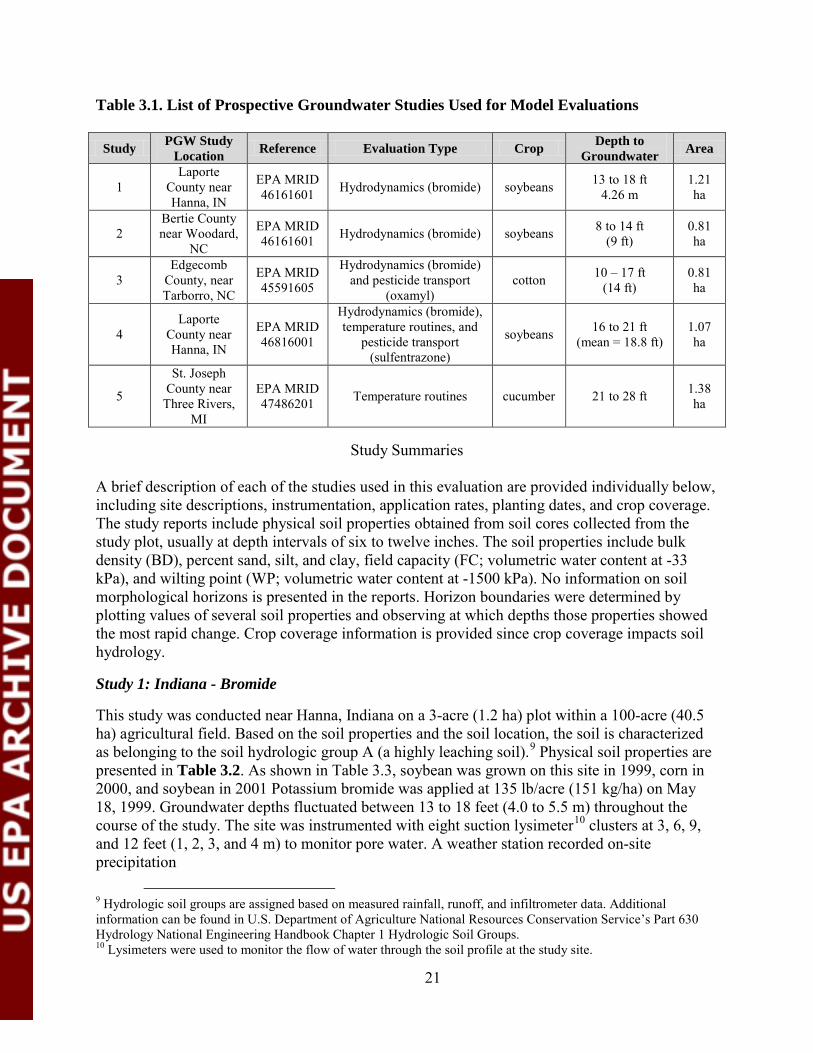
Table 3.1. List of Prospective Groundwater Studies Used for Model Evaluations

Study PGW Study Location Reference Evaluation Type Crop Depth to

Groundwater Area

1 Laporte

County near Hanna, IN

EPA MRID 46161601 Hydrodynamics (bromide) soybeans 13 to 18 ft

4.26 m 1.21 ha

2 Bertie County near Woodard,

NC

EPA MRID 46161601 Hydrodynamics (bromide) soybeans 8 to 14 ft

(9 ft) 0.81 ha

3 Edgecomb

County, near Tarborro, NC

EPA MRID 45591605

Hydrodynamics (bromide) and pesticide transport

(oxamyl) cotton 10 – 17 ft

(14 ft) 0.81 ha

4 Laporte

County near Hanna, IN

EPA MRID 46816001

Hydrodynamics (bromide), temperature routines, and

pesticide transport (sulfentrazone)

soybeans 16 to 21 ft (mean = 18.8 ft)

1.07 ha

5

St. Joseph County near

Three Rivers, MI

EPA MRID 47486201 Temperature routines cucumber 21 to 28 ft 1.38

ha

Study Summaries

A brief description of each of the studies used in this evaluation are provided individually below, including site descriptions, instrumentation, application rates, planting dates, and crop coverage. The study reports include physical soil properties obtained from soil cores collected from the study plot, usually at depth intervals of six to twelve inches. The soil properties include bulk density (BD), percent sand, silt, and clay, field capacity (FC; volumetric water content at -33 kPa), and wilting point (WP; volumetric water content at -1500 kPa). No information on soil morphological horizons is presented in the reports. Horizon boundaries were determined by plotting values of several soil properties and observing at which depths those properties showed the most rapid change. Crop coverage information is provided since crop coverage impacts soil hydrology.

Study 1: Indiana - Bromide

This study was conducted near Hanna, Indiana on a 3-acre (1.2 ha) plot within a 100-acre (40.5 ha) agricultural field. Based on the soil properties and the soil location, the soil is characterized as belonging to the soil hydrologic group A (a highly leaching soil).9 Physical soil properties are presented in Table 3.2. As shown in Table 3.3, soybean was grown on this site in 1999, corn in 2000, and soybean in 2001 Potassium bromide was applied at 135 lb/acre (151 kg/ha) on May 18, 1999. Groundwater depths fluctuated between 13 to 18 feet (4.0 to 5.5 m) throughout the course of the study. The site was instrumented with eight suction lysimeter10 clusters at 3, 6, 9, and 12 feet (1, 2, 3, and 4 m) to monitor pore water. A weather station recorded on-site precipitation

9 Hydrologic soil groups are assigned based on measured rainfall, runoff, and infiltrometer data. Additional information can be found in U.S. Department of Agriculture National Resources Conservation Service’s Part 630 Hydrology National Engineering Handbook Chapter 1 Hydrologic Soil Groups. 10 Lysimeters were used to monitor the flow of water through the soil profile at the study site.

22

Table 3.2. Study 1: Indiana Site Soil Properties

Horizon Depth (inch)

BD (g/cm3)

Sand (%)

Silt (%)

Clay (%)

FC (v/v)

WP (v/v)

1 69 1.41 0.78 0.13 0.09 0.126 0.053 2 152 1.39 0.90 0.04 0.06 0.065 0.035 3 396 1.43 0.84 0.10 0.06 0.094 0.041 4a 426 1.54 0.93 0.04 0.03 0.054 0.022 4 610 1.54 0.93 0.04 0.03 0.054 0.022

Table 3.3. Study 1: Indiana Site Crop Schedule

Crop Plant Harvest Soybean Jun. 3, 1999 Oct. 15, 1999

Corn Apr. 27, 2000 Oct. 14, 2000 Soybean May 21, 2001 Oct. 15, 2001

Study 2: North Carolina - Bromide

This study was conducted near Woodard, North Carolina on a 2-acre (0.8 ha) plot. The site lies within a 150-acre (60.7 ha) agricultural field with soil belonging to hydrologic group A. The physical soil properties for this site are provided in Table 3.4. As shown in Table 3.5, soybean was grown on this site from 1999 to 2001. Potassium bromide was applied to the field at a rate of 113 lb/acre (125 kg/ha) on April 27, 1999. Groundwater depths ranged from 8 to 14 feet (2.4 to 4.3 m). The site was equipped with eight suction lysimeter clusters at 3, 6, and 9 feet (1, 2, and 3 m) to monitor pore water. A weather station recorded on-site precipitation. Table 3.4. Study 2: Woodard, North Carolina Site Soil Properties

Horizon Depth

(inches) BD

(g/cm3) Sand (%)

Silt (%)

Clay (%)

OM (%)

FC (v/v)

WP (v/v)

1 38 1.46 0.88 0.07 0.05 0.7 0.087 0.044 2 244 1.60 0.78 0.09 0.13 0.097 4.8 0.097 3 600 1.65 0.90 0.05 0.05 0.09 2 0.064

Table 3.5. Crop Schedule for Study 1: Woodard, North Carolina Site

Crop Plant Harvest

Soybean May 11, 1999 Sept. 12, 1999 Soybean Jun. 1, 2000 Oct. 31, 2000

Soybean (surrogate for peanut) Apr. 1, 2001 Oct.8, 2001

Study 3: North Carolina – Bromide and Oxamyl

This study was conducted near Tarboro, North Carolina on a 2-acre (0.8 ha) plot. The site lies within a 4.25 acre (1.7 ha) agricultural field with soils classified as belonging to hydrologic group A. Physical soil properties for this site are provided as averages in Table 3.6. As shown in

23

Table 3.7, cotton was grown on this site in the spring of 1997 and 1998. Potassium bromide was applied at 125 lb/a (160 kg/ha) on July 1, 1997, and oxamyl was applied at 0.5 lb/a (0.56 kg/ha) on July 2, July 8, and 1.0 lb/a (1.12 kg/ha) July 14, July 22, and July 29, 1997. The site was instrumented with eight suction lysimeter clusters at 3, 6, 9, and 12 feet (1, 2, 3, and 4 m) to monitor pore water. Physical soil properties for this site are provided as averages in Table 3.6. Groundwater depths ranged from 10 to 17 feet (3.0 to 5.2 m). A weather station recorded on-site precipitation and irrigation, temperature, and wind speed.

Table 3.6. Study 3: Tarboro, North Carolina Site Soil Properties

Horizon Depth (cm)

BD (g/cm3)

Sand (%)

Silt (%)

Clay (%)

OM (%)

FC (v/v)

WP (v/v)

1 15 1.59 91.5 5 3.5 1.2 10.34 3.82 2 30 1.57 88.8 6.6 4.6 0.5 8.16 2.83 3 76 1.54 87.7 7.2 5.1 0.2 7.55 2.62 4 183 1.44 83.3 6.9 9.8 0.2 11.95 5.90 5 427 1.47 93.4 3.3 3.3 0.1 3.97 1.91

Table 3.7. Study 3: Tarboro, North Carolina Site Crop Schedule

Crop Plant Harvest cotton May 22, 1997 Nov. 15, 1997

cotton Jun. 1, 1998 (estimated, only Spring 1998) Oct. 10, 1998

Study 4: Indiana – Bromide, Temperature and Sulfentrazone

This study was conducted near Hanna, Indiana on a 2.65 acre (1.1 ha) plot (approximately four miles WNW from the site used for study 1). The site lies within an agricultural area with soils classified by hydrologic group A. The size of the treated site was not specified. Physical soil properties for this site are provided in Table 3.8. As shown in Table 3.9, wheat and soybean were grown on this site from 1999 to 2003. Groundwater depths ranged from 8 to 14 feet (2.4 to 4.3 m). Sulfentrazone was applied at a rate of 0.17 lb/acre (0.19 kg/ha), while potassium bromide was applied at a rate of 137 lb/a (154 kg/ha) on June 11, 1999. The site was instrumented with eight suction lysimeter clusters at 3, 6, 9, and 15 feet (1, 2, 3, and 5 m) to monitor pore water. A weather station recorded on-site precipitation, wind speed, and temperature. Table 3.8. Study 4: Indiana Site Soil Properties

Horizon Depth (cm)

BD (g/cm3)

Sand (%)

Silt (%)

Clay (%)

OM (%)

FC (v/v)

WP (v/v)

1 15 1.43 0.795 0.135 0.070 1.3 14 4.8 2 30 1.46 0.75 0.155 0.095 0.5 14.8 5.1 3 76 1.42 0.83 0.079 0.091 0.2 1.8 5.3 4 183 1.42 0.883 0.043 0.074 7.4 1.42 11.3 5 427 1.43 0.913 0.040 0.047 4.7 1.43 7.6

24

6 792 1.55 0.95 0.029 0.021 2.1 1.55 3.3 Table 3.9. Study 4: Indiana Site Crop Schedule

Crop Plant Date Harvest Date

Soybean Jun. 7, 1999 Oct. 15, 1999 Wheat Oct. 17, 1999 Jul. 10, 2000

Soybean May 10, 2001 Sept. 10, 2001 Wheat Sept. 20, 2001 Jul. 13, 2002

Soybean May 11, 2003 Sept. 29, 2003

Study 5: Michigan- Temperature

This study was used for temperature simulation comparisons and was conducted in southwestern Michigan, about 62 miles (100 km) NNW of Fort Wayne, Indiana. Soil properties of the site are shown in Table 3.10. The site lies in an agricultural area, with the treated site measuring 3.2 acre (1.3 ha). This study was used only for the temperature evaluation. Six temperature probes were installed for the study, the deepest of which was at 14.8 feet (4.5 m) depth. Crops, planting, and harvest times are shown in Table 3.11. Table 3.10. Study 5: Michigan Site Soil Properties

Horizon Depth (cm)

B.D. (g/cm3)

Sand (%)

Silt (%)

Clay (%)

OM (%)

FC (v/v)

WP (v/v)

1 15 1.4 81.6 9.9 8.5 1.1 8.4 3.10 2 61 1.2 82.1 9.3 8.6 0.4 6.4 2.74 3 244 1.4 93.8 1.9 4.4 0.3 3.6 1.92 4 1097 1.6 95.0 2.6 2.4 0.4 3.1 1.17

Table 3.11. Study 5: Michigan Site Crop Schedule

Crop Plant Date Harvest Date

Cucumber Jun. 14, 2001 Aug. 9, 1999 Soybeans Jun. 14, 2001 Oct. 2, 2002

Corn Apr. 20, 2003 Nov. 3, 2003 Soybeans May 19, 2004 Oct. 14, 2004

Corn Apr. 1, 2005 Not Reported

Soybeans May 1, 2006 Not Reported

(study ended May 30, 2006)

Model Parameterization

Chemical fate parameters used in the models are presented in Table 3.12. For the scenario parameters, an effort was made to select equivalent parameters for the various models.

25

Table 3.12. Model Input Values for Chemicals Used in This Evaluation

Chemical

Aerobic soil Metabolism

Half-Life (days)

Kd mL/g

Koc mL/goc

Bromide stable 0 0 Oxamyl 8.7 -- 35

Sulfentrazone 540 -- 43 Hydraulic properties of the soils were determined from the reported data, and the Rosetta pedotransfer function program (Schaap et al, 2001) was used to calculate parameters not reported. For PRZM, the field capacity was taken as the reported -33 kPa water content. For LEACHM, the retention parameters were estimated by fitting the modified Campbell (1974) equation (Hutson and Cass, 1987) used in LEACHM to the measured saturation and water contents at -33 kPa and -1500 kPa tension. Water retention curves were then estimated by regression equations that relate water retained at each of several pressure potential to soil physical properties (particle size distribution, bulk density, and organic carbon content). Parameters for the van Genuchten retention function used by PEARL were calculated using the Rosetta pedotransfer function program (Schaap et al. 2001). Rosetta was set to consider all available measurements: sand, silt and clay contents, bulk density, and -33 and -1500 kPa water contents. The ease of use of each of the models was also reported during the evaluation. This includes the model setup, maintenance and continued technical support, and simulation runtime.

Results and Discussion The following sections show the results of the field studies, including the bromide breakthrough curves at all available lysimeter depths within the unsaturated zone. In addition, the model simulation results are provided, including both individual concentrations and cumulative flow.

Hydrology Evaluation

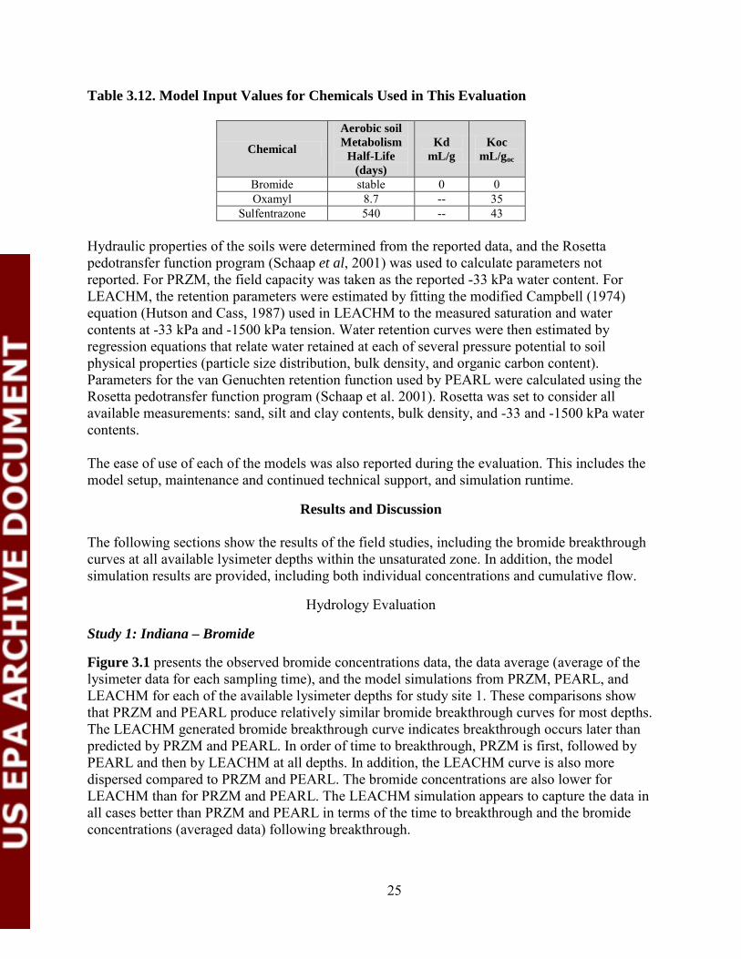
Study 1: Indiana – Bromide

Figure 3.1 presents the observed bromide concentrations data, the data average (average of the lysimeter data for each sampling time), and the model simulations from PRZM, PEARL, and LEACHM for each of the available lysimeter depths for study site 1. These comparisons show that PRZM and PEARL produce relatively similar bromide breakthrough curves for most depths. The LEACHM generated bromide breakthrough curve indicates breakthrough occurs later than predicted by PRZM and PEARL. In order of time to breakthrough, PRZM is first, followed by PEARL and then by LEACHM at all depths. In addition, the LEACHM curve is also more dispersed compared to PRZM and PEARL. The bromide concentrations are also lower for LEACHM than for PRZM and PEARL. The LEACHM simulation appears to capture the data in all cases better than PRZM and PEARL in terms of the time to breakthrough and the bromide concentrations (averaged data) following breakthrough.

26

0

10

20

30

40

50

60

70

80

90

100

0 200 400 600 800 1000

DAT

3 ft

Pore

Wat

er C

once

ntra

tion

(mg/

L)

PRZM

PEARL

LEACHM

Data Average

Data

0

10

20

30

40

50

60

70

80

90

100

0 200 400 600 800 1000

DAT

6 ft

Pore

Wat

er C

once

ntra

tion

(mg/

L)

PRZM

PEARL

LEACHM

Data Average

Data

0

10

20

30

40

50

60

70

80

90

100

0 200 400 600 800 1000

DAT

12 ft

Por

e W

ater

Con

cent

ratio

n (m

g/L) PRZM

PEARLt

LEACHM

Data Average

Data

0

10

20

30

40

50

60

70

80

90

100

0 200 400 600 800 1000

DAT

9 ft

Pore

Wat

er C

once

ntra

tion

(mg/

L)

PRZM

PEARL

LEACHM

Data Average

Data

a. b.

c. d.

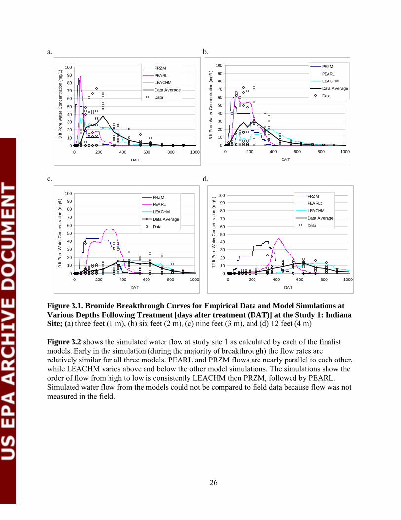
Figure 3.1. Bromide Breakthrough Curves for Empirical Data and Model Simulations at Various Depths Following Treatment [days after treatment (DAT)] at the Study 1: Indiana Site; (a) three feet (1 m), (b) six feet (2 m), (c) nine feet (3 m), and (d) 12 feet (4 m) Figure 3.2 shows the simulated water flow at study site 1 as calculated by each of the finalist models. Early in the simulation (during the majority of breakthrough) the flow rates are relatively similar for all three models. PEARL and PRZM flows are nearly parallel to each other, while LEACHM varies above and below the other model simulations. The simulations show the order of flow from high to low is consistently LEACHM then PRZM, followed by PEARL. Simulated water flow from the models could not be compared to field data because flow was not measured in the field.

27

0

0.2

0.4

0.6

0.8

1

1.2

1.4

1.6

1.8

0 200 400 600 800 1000

DAT

3 ft

Flow

(m)

PRZM

PEARL

LEACHM

0

0.2

0.4

0.6

0.8

1

1.2

1.4

1.6

1.8

0 200 400 600 800 1000

DAT

6 ft

Flow

(m)

PRZM

PEARL

LEACHM

0

0.2

0.4

0.6

0.8

1

1.2

1.4

1.6

1.8

0 200 400 600 800 1000

DAT

12 ft

Flo

w (m

)PRZM

PEARL

LEACHM

0

0.2

0.4

0.6

0.8

1

1.2

1.4

1.6

1.8

0 200 400 600 800 1000

DAT

9 ft

Flow

(m)

PRZM

PEARL

LEACHM

a. b.

c. d.

Figure 3.2. Water Flow at Various Depths Simulated Following Treatment [days after treatment (DAT)] at the Study 1 Site; (a) three feet (1 m), (b) six feet (2 m), (c) nine feet (3 m), and (d) 12 feet (4 m)

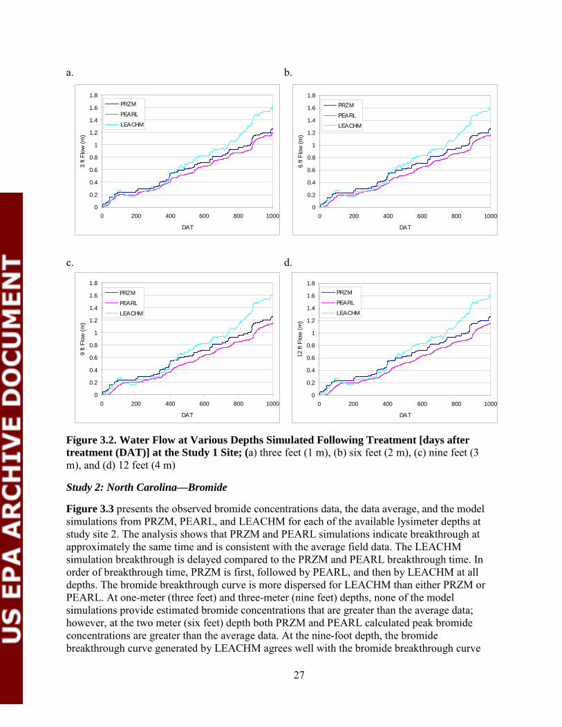
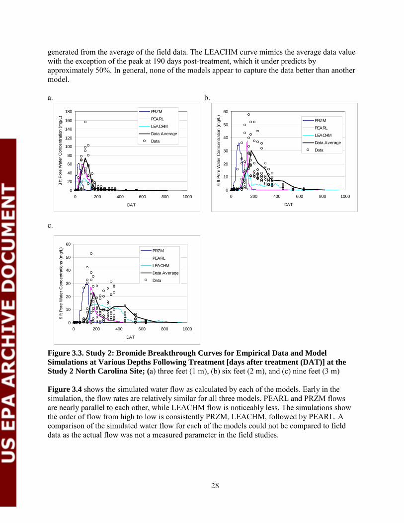
Study 2: North Carolina—Bromide

Figure 3.3 presents the observed bromide concentrations data, the data average, and the model simulations from PRZM, PEARL, and LEACHM for each of the available lysimeter depths at study site 2. The analysis shows that PRZM and PEARL simulations indicate breakthrough at approximately the same time and is consistent with the average field data. The LEACHM simulation breakthrough is delayed compared to the PRZM and PEARL breakthrough time. In order of breakthrough time, PRZM is first, followed by PEARL, and then by LEACHM at all depths. The bromide breakthrough curve is more dispersed for LEACHM than either PRZM or PEARL. At one-meter (three feet) and three-meter (nine feet) depths, none of the model simulations provide estimated bromide concentrations that are greater than the average data; however, at the two meter (six feet) depth both PRZM and PEARL calculated peak bromide concentrations are greater than the average data. At the nine-foot depth, the bromide breakthrough curve generated by LEACHM agrees well with the bromide breakthrough curve

28

0

20

40

60

80

100

120

140

160

180

0 200 400 600 800 1000

DAT

3 ft

Pore

Wat

er C

once

ntra

tion

(mg/

L)

PRZM

PEARL

LEACHM

Data Average

Data

0

10

20

30

40

50

60

0 200 400 600 800 1000

DAT

6 ft

Pore

Wat

er C

omce

ntra

tion

(mg/

L)

PRZM

PEARL

LEACHM

Data Average

Data

0

10

20

30

40

50

60

0 200 400 600 800 1000

DAT

9 ft

Pore

Wat

er C

once

ntra

tions

(mg/

L) PRZM

PEARL

LEACHM

Data Average

Data

generated from the average of the field data. The LEACHM curve mimics the average data value with the exception of the peak at 190 days post-treatment, which it under predicts by approximately 50%. In general, none of the models appear to capture the data better than another model. a. b.

c.

Figure 3.3. Study 2: Bromide Breakthrough Curves for Empirical Data and Model Simulations at Various Depths Following Treatment [days after treatment (DAT)] at the Study 2 North Carolina Site; (a) three feet (1 m), (b) six feet (2 m), and (c) nine feet (3 m)

Figure 3.4 shows the simulated water flow as calculated by each of the models. Early in the simulation, the flow rates are relatively similar for all three models. PEARL and PRZM flows are nearly parallel to each other, while LEACHM flow is noticeably less. The simulations show the order of flow from high to low is consistently PRZM, LEACHM, followed by PEARL. A comparison of the simulated water flow for each of the models could not be compared to field data as the actual flow was not a measured parameter in the field studies.

29

a. b.

c.

Figure 3.4. Water Flow at Various Depths Simulated Following Treatment [days after treatment (DAT)] at the Study 2 North Carolina Site; (a) one meter (3 feet), (b) two meters (6 feet), and (c) three meters (9 feet)

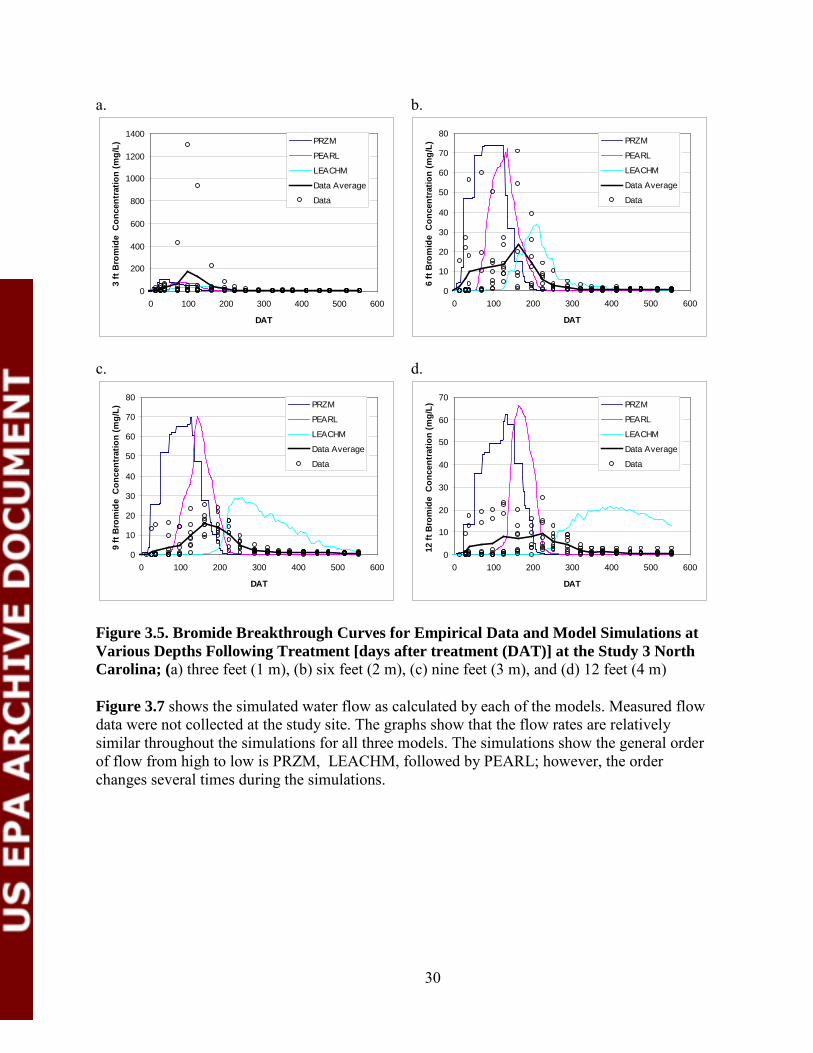
Study 3: North Carolina – Bromide and Oxamyl

Figure 3.5 presents the observed bromide concentrations data, the data average, and the model simulations from PRZM, PEARL, and LEACHM for each of the available lysimeter depths at study site 3. These comparisons show that none of the models appear to capture the data better than another model. Again, LEACHM produces a bromide breakthrough curve that is more dispersed and delayed compared to the results generated by PRZM or PEARL. For this site, the order of breakthrough time is PRZM, PEARL, and then LEACHM.

0

0.5

1

1.5

2

2.5

3

0 200 400 600 800 1000

DAT

3 ft

Flow

(m)

PRZM

PEARL

LEACHM

0

0.5

1

1.5

2

2.5

3

0 200 400 600 800 1000

DAT

6 ft

Flow

(m)

PRZM

PEARL

LEACHM

0

0.5

1

1.5

2

2.5

3

0 200 400 600 800 1000

DAT

9 ft

Flow

(m)

PRZM

PEARL

LEACHM

30

0

200

400

600

800

1000

1200

1400

0 100 200 300 400 500 600

DAT

3 ft

Bro

mid

e C

once

ntra

tion

(mg/

L)

PRZM

PEARL

LEACHM

Data Average

Data

0

10

20

30

40

50

60

70

80

0 100 200 300 400 500 600

DAT

9 ft

Bro

mid

e C

once

ntra

tion

(mg/

L)

PRZM

PEARL

LEACHM

Data Average

Data

a. b.

c. d.

Figure 3.5. Bromide Breakthrough Curves for Empirical Data and Model Simulations at Various Depths Following Treatment [days after treatment (DAT)] at the Study 3 North Carolina; (a) three feet (1 m), (b) six feet (2 m), (c) nine feet (3 m), and (d) 12 feet (4 m)

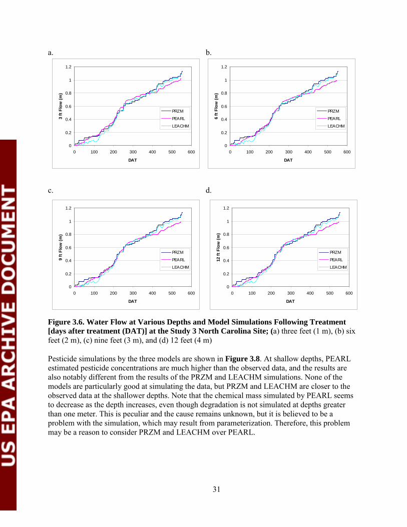
Figure 3.7 shows the simulated water flow as calculated by each of the models. Measured flow data were not collected at the study site. The graphs show that the flow rates are relatively similar throughout the simulations for all three models. The simulations show the general order of flow from high to low is PRZM, LEACHM, followed by PEARL; however, the order changes several times during the simulations.

0

10

20

30

40

50

60

70

80

0 100 200 300 400 500 600

DAT

6 ft

Bro

mid

e C

once

ntra

tion

(mg/

L)

PRZM

PEARL

LEACHM

Data Average

Data

0

10

20

30

40

50

60

70

0 100 200 300 400 500 600

DAT

12 ft

Bro

mid

e C

once

ntra

tion

(mg/

L) PRZM

PEARL

LEACHM

Data Average

Data

31

0

0.2

0.4

0.6

0.8

1

1.2

0 100 200 300 400 500 600

DAT

6 ft

Flo

w (m

)

PRZM

PEARL

LEACHM

0

0.2

0.4

0.6

0.8

1

1.2

0 100 200 300 400 500 600

DAT

3 ft

Flo

w (m

)

PRZM

PEARL

LEACHM

0

0.2

0.4

0.6

0.8

1

1.2

0 100 200 300 400 500 600

DAT

12 ft

Flo

w (m

)

PRZM

PEARL

LEACHM

a. b.

c. d.

Figure 3.6. Water Flow at Various Depths and Model Simulations Following Treatment [days after treatment (DAT)] at the Study 3 North Carolina Site; (a) three feet (1 m), (b) six feet (2 m), (c) nine feet (3 m), and (d) 12 feet (4 m)

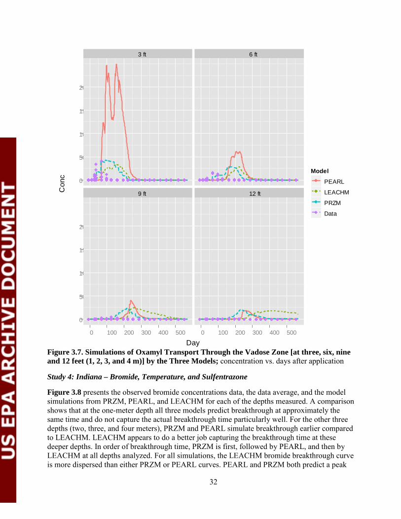
Pesticide simulations by the three models are shown in Figure 3.8. At shallow depths, PEARL estimated pesticide concentrations are much higher than the observed data, and the results are also notably different from the results of the PRZM and LEACHM simulations. None of the models are particularly good at simulating the data, but PRZM and LEACHM are closer to the observed data at the shallower depths. Note that the chemical mass simulated by PEARL seems to decrease as the depth increases, even though degradation is not simulated at depths greater than one meter. This is peculiar and the cause remains unknown, but it is believed to be a problem with the simulation, which may result from parameterization. Therefore, this problem may be a reason to consider PRZM and LEACHM over PEARL.

0

0.2

0.4

0.6

0.8

1

1.2

0 100 200 300 400 500 600

DAT

9 ft

Flo

w (m

)

PRZM

PEARL

LEACHM

32

Figure 3.7. Simulations of Oxamyl Transport Through the Vadose Zone [at three, six, nine and 12 feet (1, 2, 3, and 4 m)] by the Three Models; concentration vs. days after application

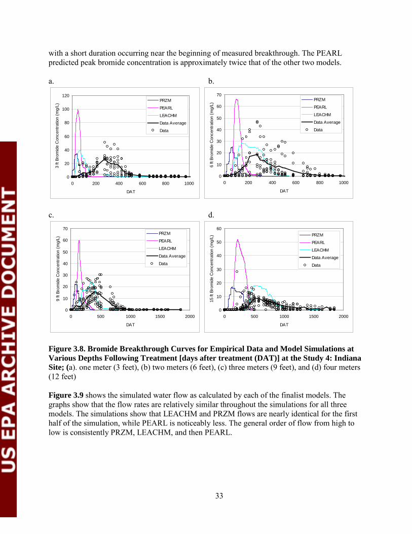
Study 4: Indiana – Bromide, Temperature, and Sulfentrazone

Figure 3.8 presents the observed bromide concentrations data, the data average, and the model simulations from PRZM, PEARL, and LEACHM for each of the depths measured. A comparison shows that at the one-meter depth all three models predict breakthrough at approximately the same time and do not capture the actual breakthrough time particularly well. For the other three depths (two, three, and four meters), PRZM and PEARL simulate breakthrough earlier compared to LEACHM. LEACHM appears to do a better job capturing the breakthrough time at these deeper depths. In order of breakthrough time, PRZM is first, followed by PEARL, and then by LEACHM at all depths analyzed. For all simulations, the LEACHM bromide breakthrough curve is more dispersed than either PRZM or PEARL curves. PEARL and PRZM both predict a peak

Day

Con

c

0

500

1000

1500

2000

0

500

1000

1500

2000

3 ft

9 ft

0 100 200 300 400 500

6 ft

12 ft

0 100 200 300 400 500

Model

PEARL

LEACHM

PRZM

Data

33

with a short duration occurring near the beginning of measured breakthrough. The PEARL predicted peak bromide concentration is approximately twice that of the other two models. a. b.

c. d.

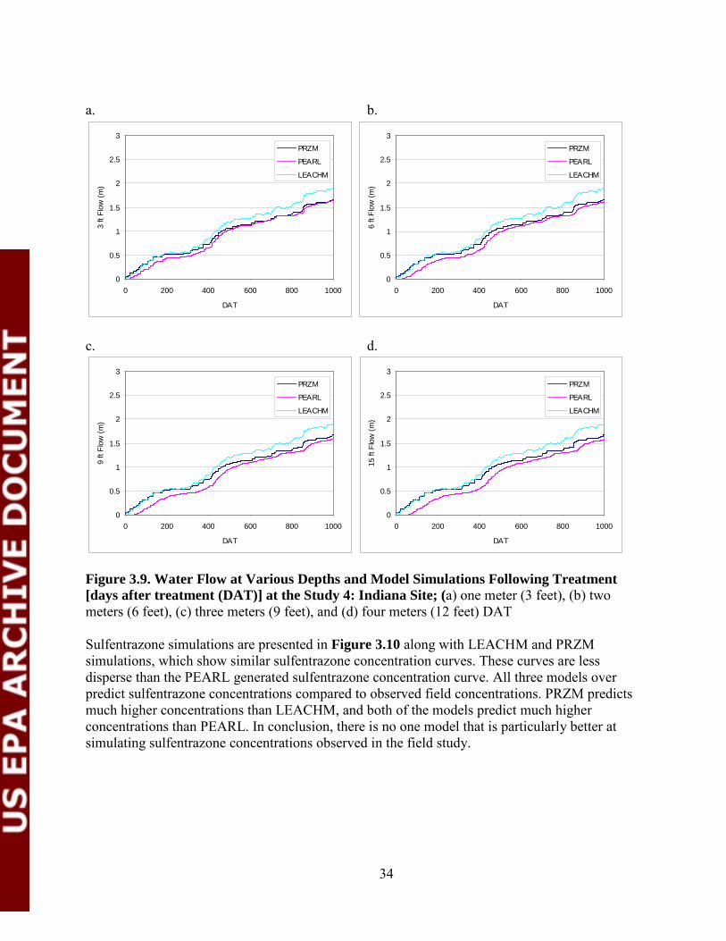
Figure 3.8. Bromide Breakthrough Curves for Empirical Data and Model Simulations at Various Depths Following Treatment [days after treatment (DAT)] at the Study 4: Indiana Site; (a). one meter (3 feet), (b) two meters (6 feet), (c) three meters (9 feet), and (d) four meters (12 feet) Figure 3.9 shows the simulated water flow as calculated by each of the finalist models. The graphs show that the flow rates are relatively similar throughout the simulations for all three models. The simulations show that LEACHM and PRZM flows are nearly identical for the first half of the simulation, while PEARL is noticeably less. The general order of flow from high to low is consistently PRZM, LEACHM, and then PEARL.

0

20

40

60

80

100

120

0 200 400 600 800 1000

DAT

3 ft

Brom

ide

Con

cent

ratio

n (m

g/L)

PRZM

PEARL

LEACHM

Data Average

Data

0

10

20

30

40

50

60

70

0 200 400 600 800 1000

DAT

6 ft

Brom

ide

Con

cent

ratio

n (m

g/L)

PRZM

PEARL

LEACHM

Data Average

Data

0

10

20

30

40

50

60

70

0 500 1000 1500 2000

DAT

9 ft

Brom

ide

Con

cent

ratio

n (m

g/L)

PRZM

PEARL

LEACHM

Data Average

Data

0

10

20

30

40

50

60

0 500 1000 1500 2000

DAT

15 ft

Bro

mid

e C

once

ntra

tion

(mg/

L) PRZM

PEARL

LEACHM

Data Average

Data

34

a. b.

c. d.

Figure 3.9. Water Flow at Various Depths and Model Simulations Following Treatment [days after treatment (DAT)] at the Study 4: Indiana Site; (a) one meter (3 feet), (b) two meters (6 feet), (c) three meters (9 feet), and (d) four meters (12 feet) DAT Sulfentrazone simulations are presented in Figure 3.10 along with LEACHM and PRZM simulations, which show similar sulfentrazone concentration curves. These curves are less disperse than the PEARL generated sulfentrazone concentration curve. All three models over predict sulfentrazone concentrations compared to observed field concentrations. PRZM predicts much higher concentrations than LEACHM, and both of the models predict much higher concentrations than PEARL. In conclusion, there is no one model that is particularly better at simulating sulfentrazone concentrations observed in the field study.

0

0.5

1

1.5

2

2.5

3

0 200 400 600 800 1000

DAT

3 ft

Flow

(m)

PRZM

PEARL

LEACHM

0

0.5

1

1.5

2

2.5

3

0 200 400 600 800 1000

DAT

6 ft

Flow

(m)

PRZM

PEARL

LEACHM

0

0.5

1

1.5

2

2.5

3

0 200 400 600 800 1000

DAT

9 ft

Flow

(m)

PRZM

PEARL

LEACHM

0

0.5

1

1.5

2

2.5

3

0 200 400 600 800 1000

DAT

15 ft

Flo

w (m

)PRZM

PEARL

LEACHM

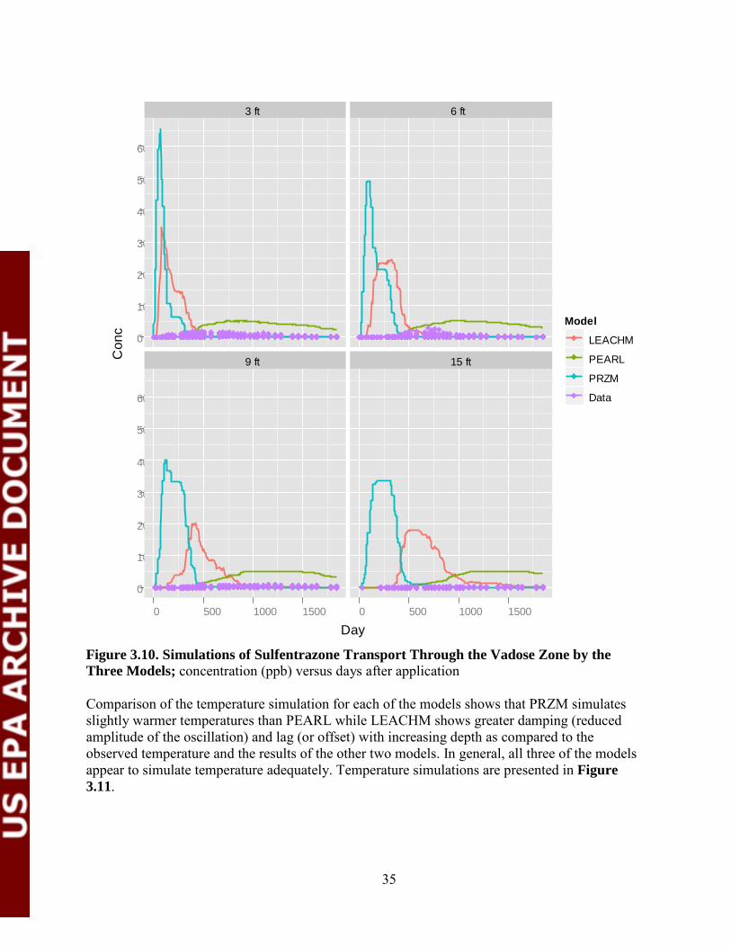
35

Figure 3.10. Simulations of Sulfentrazone Transport Through the Vadose Zone by the Three Models; concentration (ppb) versus days after application Comparison of the temperature simulation for each of the models shows that PRZM simulates slightly warmer temperatures than PEARL while LEACHM shows greater damping (reduced amplitude of the oscillation) and lag (or offset) with increasing depth as compared to the observed temperature and the results of the other two models. In general, all three of the models appear to simulate temperature adequately. Temperature simulations are presented in Figure 3.11.

Day

Con

c

0

10

20

30

40

50

60

0

10

20

30

40

50

60

3 ft

9 ft

0 500 1000 1500

6 ft

15 ft

0 500 1000 1500

Model

LEACHM

PEARL

PRZM

Data

36

Figure 3.11. Temperature Simulation Comparison at the Study 4: Indiana Site for Depths of 4 and 24 Inches. The graph shows soil temperature measured at the weather station (black) and LEACHM (blue), PRZM (magenta), and PEARL (green) simulations

Study 5: Michigan Temperature

Temperature simulations for the Michigan site are presented in Figure 3.12. Results indicate that both PRZM and PEARL are better than LEACHM for simulating temperature at this site. The yearly temperature oscillations in the LEACHM simulations are both more damped and delayed compared to field measurements and the other two model results. For this reason, LEACHM is not considered the optimal model for temperature simulations. The largest difference between PRZM and PEARL temperature simulation results occur at times when the soil is frozen. PEARL seems to predict colder soil temperatures compared to the measured data, while PRZM does not allow the temperature to drop below zero. Field measurements include sub-zero temperatures, but the field measured values are both fewer and warmer than those simulated by PEARL, making the PRZM simulations more accurate. Since pesticide degradation is generally very slow at temperatures near and below zero, the differences in the handling of the zero temperature of the models will have little effect on the estimated pesticide concentrations. In general, the PRZM and PEARL predicted soil temperature similarly; therefore, either model will provide an adequate temperature simulation for modelling pesticide leaching.

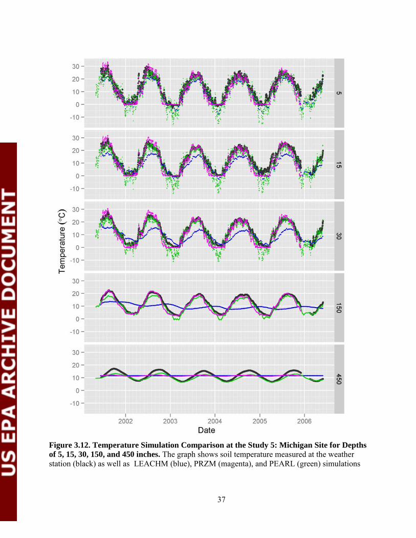
37

Figure 3.12. Temperature Simulation Comparison at the Study 5: Michigan Site for Depths of 5, 15, 30, 150, and 450 inches. The graph shows soil temperature measured at the weather station (black) as well as LEACHM (blue), PRZM (magenta), and PEARL (green) simulations

38

Ease of Use Evaluation

During the course of the evaluation presented above it became clear that the models required different levels of expertise (and patience) to operate properly. PRZM was by far the easiest to populate and run, while PEARL was the most difficult to populate and run. Excessive layering of PEARL inputs through multiple windows was not intuitive to all users. In addition, during simulation, several PEARL forced shutdowns occurred. Maintenance and ownership questions also arose when problems were encountered during the simulations. In-house expertise on PRZM facilitated PRZM’s use, while LEACHM and PEARL assistance was only available through email contact with the overseas developers, which was not convenient.

Summary No single model stands out as the best in terms of the ability to accurately simulate water flow, pesticide concentration, and soil temperature; therefore, all models could clearly be applied adequately as a tool to simulation pesticide transport to groundwater. However, during the course of the simulation evaluation, it became clear that PRZM was easier to operate and maintain. In conclusion, after a review of the model performance, maintenance and ease-of-use issues, PRZM was selected as the most appropriate tool for implementation of the groundwater conceptual model presented in Chapter 1. Additional analysis of PRZM for use in simulating pesticide concentration for regulatory purposes is provided in the following chapter.

References

Campbell, G. 1974. A simple method for determining unsaturated conductivity from moisture retention data. Soil Sci. 117:311-314. Brooks, R.H. and Corey, A.T., 1964. Hydraulic properties of porous media. In: Hydrol. Paper no. 3, Civ. Eng. Dept., Colorado State Univ., Fort Collins, CO. Hutson,J . L., Cass, A. A retentivity function or use in soil-water simulation models, J. Soil Sci. 8, 105-113, 1987. Schaap, M.G., Leij, F.J., van Genuchten M.Th. 2001. Rosetta: a computer program for estimating soil hydraulic parameters with hierarchical pedotransfer functions. Journal of Hydrology, 251, 163-176.

39

Chapter 4: PRZM MODEL EVALUATION USING GROUNDWATER MONITORING DATA

PRZM performs two general roles for regulatory assessments: it performs as a screen to flag chemicals that need further examination, and it is used to evaluate the impact of refinements and mitigation options on those flagged chemicals. To evaluate PRZM in these two modes, both non-targeted and targeted monitoring data are compared to various types of PRZM simulations. This chapter describes the details of these evaluations.

Method Overview

An effective groundwater screening tool simulates pesticide concentrations greater than those observed in the vast majority of drinking water wells. In cases when the screen underestimates the observed concentrations, those observations must be examined to ensure that these underestimated values will not result in public harm. To determine the effectiveness of PRZM, five different data sets that comprised both targeted groundwater monitoring sites and non-targeted monitoring sites were compared to PRZM simulation outputs from the six standard scenarios.11 The scenarios were developed to represent known areas with vulnerable drinking water sources, and the locations are highlighted in Figure 4.1. The non-targeted sites were used to evaluate the screening abilities of PRZM, and the targeted sites were used to test the refinement capabilities of PRZM.

Figure 4.1. PRZM Groundwater Scenario Locations

11 Florida Citrus (FLC), Florida Potato (FLP), Wisconsin Corn (WIC), Georgia Peanuts (GAP), North Carolina Cotton (NCC), and Delmarva Sweet Corn (DEL)

40

The following large-scale multi-site monitoring studies were selected for use in this evaluation:

• The National Water Quality Assessment (NAWQA) Program (US Geological Survey) • The Acetochlor Registration Partnership (ARP) Midwest Corn Production Area

(MwCPA) Monitoring Program (also known as the ARP State Ground-Water Monitoring Program)

• The National Alachlor Well-Water Survey (NAWWS) submitted to EPA by Monsanto Company to support alachlor registration.

Two site-specific assessments selected for use in this evaluation are: • The North Carolina Prospective Groundwater (PGW) monitoring study for oxamyl;

submitted to the EPA by E.I. du Pont de Nemours and Company to support registration of oxamyl.

• Selected USDA Pesticide Data Program California monitoring results for diuron matched with California Department of Pesticide Regulation’s Pesticide Use Reporting data.

These datasets each have different advantages and limitations for use in pesticide groundwater exposure model evaluations. A discussion of each of the monitoring programs is provided below, including the rationale for selecting each dataset. Additionally, model output concentrations for the chemicals detected in the NAWQA program dataset were compared to the publically available list of Human Health Benchmarks for Pesticides (http://iaspub.epa.gov/apex/pesticides/f?p=HHBP:home). The comparison of screening-level model results with benchmarks for human health indicates how often higher level refinements may be needed.

Monitoring Program Summaries

National Water Quality Assessment (NAWQA) Program

Overview

The NAWQA program provides a nationally relevant dataset that includes analytes from a large list of pesticides and pesticide degradation products, larger than any other monitoring program of its scope and duration. However, the dataset is limited in that each of the 59 NAWQA Study Units (SU) have multiple objectives and are not specifically designed to evaluate the impacts of pesticide usage on drinking water supplies (e.g., groundwater used as source drinking water).12 More than half of the NAWQA groundwater monitoring sites are used as domestic and public drinking water; however, this evaluation did not specifically distinguish between observed concentrations in drinking water supply wells versus other observation wells included in the NAWQA program.

12 Gilliom et al. (2006) provides an overall perspective on the pesticide monitoring program. Domestic well water monitoring results are summarized in DeSimone et al. (2009) and public well water supply results are presented in Toccalino and Hopple (2010). For more information on the NAWQA program web citations are provided in the References section of this chapter.

41

The NAWQA program has estimates of agricultural pesticide usage by crop and by state (and sometimes by county) over the course of the monitoring program; however, it is still not possible for this assessment to estimate usage in the zone of influence for each monitored well over the entire time scale that is relevant to the observed concentrations. Often pesticide usage for decades prior to the sampling date is needed to accurately associate usage of a specific pesticide with what might be observed in a groundwater sample. In addition, NAWQA well locations are diverse and include urban watersheds and other areas where few or no pesticides are used. While extensive, the NAWQA program does not encompass the entire United States, capture all agricultural areas, or capture all high pesticide use areas. Therefore, the observed concentrations may not represent the highest groundwater concentrations that could be observed for a particular pesticide. The NAWQA program study units do not specifically target vulnerable groundwater supplies (i.e., wells drawing from an unconfined high water-table aquifer in high pesticide use areas—similar to the conceptual model implemented in PRZM). In some study areas the aquifers sampled by NAWQA wells are deeper and more confined than in the conceptual model. Only a subset of the NAWQA measurements are from shallow, unconfined aquifers similar to the conceptual model. For example, 75% of the wells were drilled to a depth greater than 31 feet and, for sites with such information, 75% of the wells were screened starting at >20 feet below ground surface (bgs) and 50% at >50 feet bgs13. Ancillary data concerning well characteristics (e.g., depth to groundwater) and groundwater properties are typically available for samples sites included in the NAWQA dataset, and these data could permit additional evaluation and characterization. However, this characterization was not completed. Only positive detections in groundwater were used in this evaluation. Detections of degradate compounds and canceled pesticides were not included in this analysis. In total, 66 chemicals were used in this evaluation. These 66 chemicals were reported as detections in groundwater by NAWQA regardless of the frequency of detections (50 of these compounds had 5 or more detections).

Use and Limitations A comparison of PRZM estimated pesticide concentrations to NAWQA pesticide detections provides insight into the model performance as a regulatory screen. However, because specific monitoring site analyses are not a part of this effort, the degree of over- or under-prediction of specific simulated values to the observed values is not meaningful and therefore our focus was on overall comparisons in order to assess model screening efficiency. Such a comparison is not appropriate because the PRZM model was not parameterized to simulate each of the NAWQA sites, especially in regard to the pesticide usage at the sites. The PRZM-simulated concentrations resulting from the use of the highly vulnerable standard scenarios are expected to be greater than the NAWQA detections as the vulnerability of the NAWQA monitoring sites is uncertain and likely less vulnerable than the standard scenarios which are based upon the most vulnerable

13 Source: Download on 6/4/2012 of well site data from the NAWQA Data Warehouse at:

http://infotrek.er.usgs.gov/nawqa_queries/jsp/sitemaster.jsp. Well screening depths were recorded for 89% of the sites.

42

groundwater in the entire United States. In this report, the PRZM simulation results are only compared with the high-end distribution of concentrations observed in NAWQA wells. This comparison was conducted in order to evaluate the ability of the conceptual model as implemented in PRZM to provide a protective screen for pesticide concentrations with varying physical chemical properties in groundwater wells on a national scale.

43

Acetochlor Registration Partnership (ARP) Midwest Corn Production Area (MwCPA) Program

Overview

The ARP MwCPA program is a large-scale targeted monitoring study that evaluated groundwater concentrations of several pesticides used heavily on corn (acetochlor, alachlor, atrazine, and metolachlor) in the United States, mainly Midwestern corn production areas. These herbicides have relatively similar use patterns and fall within a relatively narrow range of environmental fate properties (i.e., mobility and persistence properties) and are among the most commonly detected in groundwater. Sampled well locations were paired with the specific usage information from up gradient fields. The use intensity of the pesticide analytes were well defined during the course of the study. The advantage of this study is that concentrations in groundwater were measured at regular sampling intervals for each well over a seven-year period. Therefore, exposure can be analyzed on a short- and a more long-term basis. Detailed ancillary data concerning well characteristics (e.g., screening depth) and groundwater properties are available for this study since all of the monitoring wells were installed specifically for this study and the well characteristic data were recorded. Nevertheless, additional analysis, taking into account this ancillary data, was not completed as part of this evaluation. Although these chemicals are not the most mobile chemicals included in this evaluation, these chemicals are each classified as “mobile” or on the low (mobile) end of the “moderately mobile” FAO classification14 and have historically been among the most commonly detected in U.S. groundwater over the last few decades. In addition, these chemicals are believed to be used widely throughout the study area. Therefore, the chemicals included in this study are a good choice for comparison of more extreme exposure scenarios. Another advantage of this study is that temporal variability in residues was examined with regular sampling over a 7-year period at each site, facilitating evaluation of longer term exposure estimates with the model estimated concentrations.

Use and Limitations

Comparing the PRZM predicted pesticide concentrations to the ARP MwCPA dataset produces a more detailed picture of how modeling predictions compare to environmental concentrations in groundwater because contextual pesticide use information is available. The use history of acetochlor is known for the zone of influence for the time preceding the study as well as during the study period; however, the use history for the other three pesticides is not as robust, and some assumptions were made regarding the use of these pesticides for modeling purposes. In addition, despite having information on the pesticide use history for the pesticides included in this study, it is still likely that modeling assumptions differ from actual conditions. The PRZM-simulated

14 See: For example: “Guidance for Reporting on the Environmental Fate and Transport of the Stressors of Concern in Problem Formulations for Registration Review, Registration Review Risk Assessments, Listed Species Litigation Assessments, New Chemical Risk Assessments, and Other Relevant Risk Assessments”; EPA / OPP / EFED Memorandum dated 1/25/2010.

44

concentrations resulting from the use of the highly vulnerable standard scenarios are expected to be greater than the ARP detections as the vulnerability of the individual monitoring sites is uncertain and possibly less vulnerable than the standard scenarios. The relatively narrow range of environmental fate properties, use patterns of the analytes examined, and the potential difference in the vulnerability of the monitoring sites compared to the scenarios used in the PRZM simulations used in this evaluation limits the assessment of PRZM performance for pesticides with different environmental fate property profiles and different use patterns. National Alachlor Well-Water Survey (NAWWS)

Overview

The NAWWS study, like the ARP MwCPA study, focused on high use areas for the pesticides alachlor, atrazine, and metolachlor. The sampled wells from the NAWWS study were existing private drinking water wells down gradient of agricultural fields with a history of use for the identified herbicides (Holden et al. (1988, 1992), and Liddle et al. (1990)). The focus of the study design was to target wells in alachlor use areas; however, the use area for atrazine and metolachlor coincided with the alachlor use area so they were included in the survey. The survey design included sampling of 1,430 different wells one time. Sample sites were weighted towards those wells drawing from more vulnerable groundwater supplies. Ancillary data concerning well characteristics (e.g., screening depth) and groundwater properties was available to a limited extent. An advantage of the NAWWS study with respect to evaluation of PRZM use in drinking water exposure assessments is that this study focused exclusively on private drinking water wells. These types of wells are more likely to be vulnerable to contamination from pesticide applications compared to public water supply wells (e.g., private wells are more likely to be screened into shallow, unconfined, surficial aquifers).

Use and Limitations While the monitoring sites are known drinking water wells, it is unclear if these sites are highly vulnerable to pesticide leaching; therefore, the PRZM-simulated concentrations resulting from the use of the highly vulnerable standard scenarios maybe greater than the NAWWS observed concentrations. The NAWWS study does not provide direct information on temporal variability of groundwater concentrations as only one sample was taken; therefore, analysis of peak and long term exposure is limited to comparisons with the maximum / high-end measured concentrations over all sites. As a result, model performance for longer term exposure estimations is not possible.

North Carolina PGW Study

Overview

45

E.I. du Pont de Nemours and Company commissioned a small-scale prospective groundwater monitoring study designed to evaluate the potential of oxamyl and its degradate oxamyl oxime to contaminate groundwater contamination at a vulnerable site cropped with cotton. The study site, located in Tarboro, Edgecombe County, North Carolina (Southeast Atlantic Coastal Plain region of the United States), was selected based on soil and hydrogeologic criteria regarding vulnerability of the site to leaching. The study was submitted to EPA in support of the continued registration of oxamyl. Oxamyl hydrolysis is pH dependent. This is the same study that was used in Chapter 3. In Chapter 3, this study was used to evaluate pore water, whereas in this chapter the study was used to analyze pesticide concentrations in groundwater.

Use and Limitations

Since the oxamyl hydrolysis is pH dependent, examination of the hydrolysis input parameter can be evaluated. This is a relatively short (two-year) study, where measurable concentrations of oxamyl were reported in groundwater with reasonable breakthrough. However, the long term leaching potential of oxamyl cannot be assessed.

USDA PDP

Overview In 1991, the United States Department of Agriculture (USDA) was charged with designing and implementing a program to collect data on pesticide residues in food. Responsibility for this program was given to the USDA Agricultural Marketing Service (AMS), which began operating the Pesticide Data Program (PDP) in May 1991. The data produced by PDP are reported in an annual summary. The PDP database contains monitoring data from private and school well water and municipal drinking water. Select PDP data for diuron detections in Fresno, California were compared to refined PRZM model simulations. Additional usage data and chemical fate properties from the California Department of Pesticide Regulation (CalDPR) and the CalDPR’s Pesticide Use Reporting (PUR) database were used to refine model inputs.

Use and Limitations

Generally, PDP monitoring data lacks pesticide usage data; however, the PDP data for the site in Fresno, CA was supplemented with usage data from the PUR database to evaluate PRZM modeling with refined input parameters, including pesticide use intensity, hydrolysis and aerobic soil metabolism rate constants.

Model Parameterization Chemical specific model input values (e.g., chemical half-live values, maximum application rates, minimum retreatment intervals)15 were obtained from the most recent U.S. EPA drinking

15 Application rate and frequency were obtained from the most recent USEPA Drinking Water Exposure Assessment, which typically assesses the maximum application rate permitted by the registered label (consistent with USEPA/OPP policy).

46

water exposure assessment and were developed in accordance with the current input parameter guidance (USEPA 2009)16 except for the site-specific modeling conducted for oxamyl and diuron. A summary of the fate input values used for each pesticide modeled is provided in Table 4.1 with all the values provided in APPENDIX A. To ensure accuracy, individual EFED chemical teams were asked to confirm the accuracy of the model input values. Modeling assumed maximum pesticide application every year, in accordance with the pesticide label for the duration of the simulation unless otherwise noted. Table 4.1. Range of Fate Parameters Used in the Evaluation

Hydrolysis Half-life Aerobic Soil Metabolism Half-life Sorption Coefficent

1.8-300 days 0 (i.e., stable; n=54)

0.5-2940 days (3x; n=16)

7.7-30820 (Koc) 0.12-7.6 (kd)

The model was run for each pesticide using each of the six standard scenario locations: Florida Citrus (FLC), Florida Potato (FLP), Wisconsin Corn (WIC), Georgia Peanuts (GAP), North Carolina Cotton (NCC), and Delmarva Sweet Corn (DEL). These scenarios were developed based on the conceptual model (i.e., rural, shallow, unconfined aquifer in the vicinity of an agricultural field receiving a pesticide application). Model runs were completed in batches where every chemical was run through every scenario for 30 and 100- year simulations. The output was post-processed in Microsoft Excel® to produce the graphical output of all chemicals and efficiently complete the analyses.

Modeling and Monitoring Data Comparison

PRZM is a computer model that generates exposure estimates for drinking water using laboratory data that describe how fast a pesticide breaks down or transforms to other chemicals and how the pesticide is transported through the soil profile by water. Furthermore, the conceptual model does not represent all drinking water well sites. Monitoring data can elucidate what is happening under current use practices and under typical conditions. Although monitoring data can provide a direct estimate of the concentration of a pesticide in water, it does not always provide a reliable estimate of exposures because sampling may not occur where the highest pesticide concentrations are found, and sampling may not occur in locations most vulnerable to pesticide contamination. Therefore, direct comparisons of modeling and monitoring should be done with caution as these data represent different types of information. The modeling output represents 30 and 100 years of pesticide application every year over the simulation period. Where breakthrough did not occur with a 30-year simulation, the chemical-scenario combination was run for 100 years. The NAWQA dataset does not contain contextual information on pesticide use, and it is not likely that pesticides would have historically been used at the maximum frequency, rate and intensity as modeled (application every year). The comparison was used as a screen against non-targeted monitoring in the context of a regulatory assessment of drinking water exposure (i.e., the maximum labeled rate for the entire simulation). The MwCPA and NAWWS datasets are directly or indirectly targeted monitoring studies for

16 Guidance for Selecting Input Parameters in Modeling the Environmental Fate and Transport of Pesticides, Version 2.1, October 22, 2009.

47

certain high-use herbicides and, therefore, the monitoring data provide more of a direct comparison to model output data particularly when the use intensity is modified to better simulate the history of use at the monitoring sites. It should be reiterated that while these studies are targeted and use information is provided, the actual pesticide use is still significantly lower than the modeled rate for the simulation unless otherwise noted. Comparisons made to the NAWQA and NAWWS datasets are intended for short-term exposures; however, the monitoring data may not represent peak concentrations that could be observed in all groundwater supplies. The MwCPA dataset (intensive monitoring over a seven-year period) permits a longer term exposure comparison. In an effort to address the disparity between non-targeted monitoring data and model runs, further analysis was completed for site-specific model runs. The site-specific model runs were completed for the North Carolina PGW monitoring study for oxamyl. For this analysis a site-specific scenario was developed using the soil properties reported in the study, and local weather data was used for PRZM modeling. An additional comparison was made with the PDP data for diuron relative to a PRZM modeling conducted as a screening-tool and a refined analysis.

Results and Discussion

National Water Quality Assessment (NAWQA) Program

The maximum PRZM simulated pesticide concentrations were above the maximum reported concentration for most chemicals across the six simulated standard scenarios (Figure 4.2). For some chemicals, the ratio of the model predicted concentrations to the highest detected concentration reported in the NAWQA data set is >100x. The majority of the chemicals that PRZM predicts higher (>100x) concentrations than the reported concentration are persistent to very persistent (half-life values ranging from [> 100 days]) and are lower-sorbing compounds (Koc < 400 mL/goc). Chemicals with these characteristics are expected to leach to groundwater; therefore, it is important not to underestimate the concentration of these chemicals in groundwater. For several chemicals, the NAWQA dataset concentrations were greater than those predicted by PRZM.17 Of the 66 pesticides in the NAWQA dataset, 11peak pesticide detections were higher than those predicted using PRZM considering the peak simulated concentration from all the standard scenarios (for 30- or 100-year simulations18) as shown in Figure 4.2. The number of chemicals PRZM simulated concentrations that were lower than the observed concentrations across the six standard scenarios ranged from 11 to 31 (Figure 4.3). Most of the PRZM predictions that were lower than the observed detections were from the North Carolina cotton (n=22) and Florida potato (n=31) scenarios. This analysis highlights the difference in the vulnerability of the standard scenarios.

17 Benfluralin, cypermethrin, triallate, iprodione (most), parathion, chlorpyrifos (most), ethafluralin, glyphosate, propyzamide, carbaryl, dichlobenil, bentazon. 18 When breakthrough was not observed (throughputs <1) for a 30-year simulation, a second simulation was completed for 100 years. This is referred to as the “hybrid” approach.

48

Figure 4.2. Highest PRZM-simulated Concentrations (of all six standard scenarios) Compared with the Highest NAWQA Detections

49

a. b.

c. d.

e. f.

Figure 4.3. PRZM-simulated Concentration (for 30 or 100 years) and Highest NAWQA Reported Detection Log-Log Scale Plots for the Six Standard Scenarios; The solid line is the 1:1 line of predicted versus observed (PRZM-simulated values less than 0.0001 ppb are reported as 0.0001 ppb for graphical purposes)

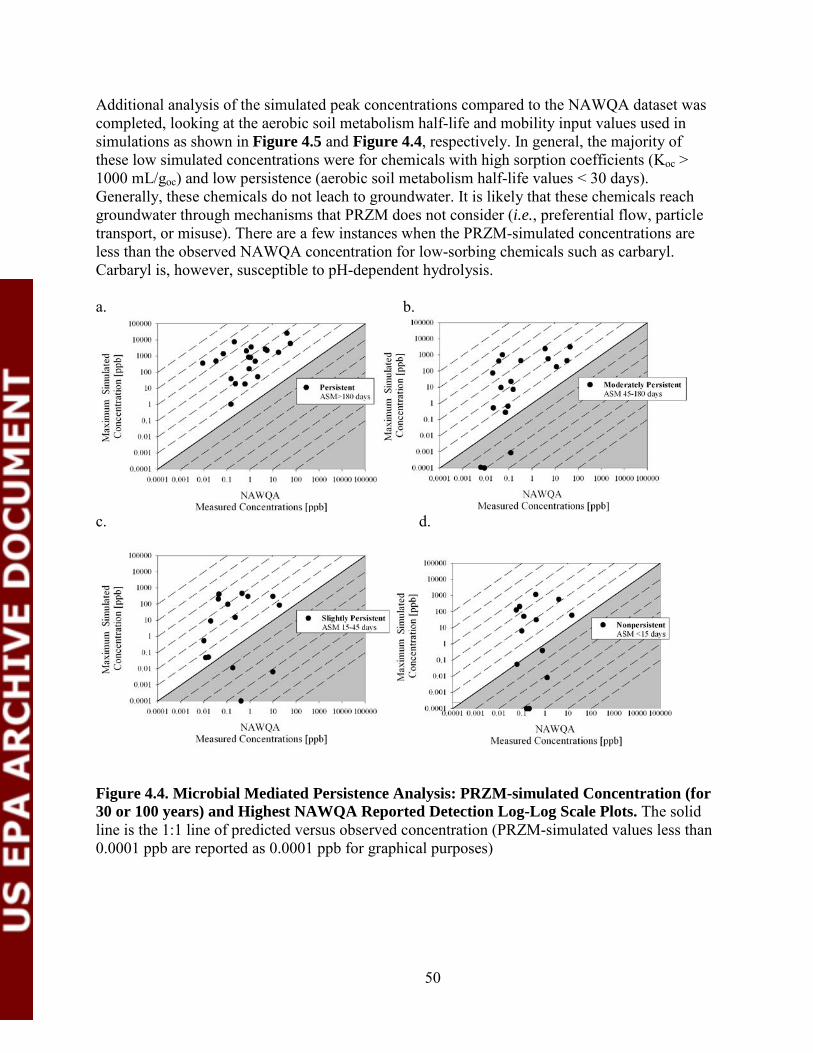
50

Additional analysis of the simulated peak concentrations compared to the NAWQA dataset was completed, looking at the aerobic soil metabolism half-life and mobility input values used in simulations as shown in Figure 4.5 and Figure 4.4, respectively. In general, the majority of these low simulated concentrations were for chemicals with high sorption coefficients (Koc > 1000 mL/goc) and low persistence (aerobic soil metabolism half-life values < 30 days). Generally, these chemicals do not leach to groundwater. It is likely that these chemicals reach groundwater through mechanisms that PRZM does not consider (i.e., preferential flow, particle transport, or misuse). There are a few instances when the PRZM-simulated concentrations are less than the observed NAWQA concentration for low-sorbing chemicals such as carbaryl. Carbaryl is, however, susceptible to pH-dependent hydrolysis. a. b.

c. d.

Figure 4.4. Microbial Mediated Persistence Analysis: PRZM-simulated Concentration (for 30 or 100 years) and Highest NAWQA Reported Detection Log-Log Scale Plots. The solid line is the 1:1 line of predicted versus observed concentration (PRZM-simulated values less than 0.0001 ppb are reported as 0.0001 ppb for graphical purposes)

51

a. b.

c. d.

e.

Figure 4.5. Mobility Analysis: PRZM-simulated Concentration (for 30 or 100 years) and Highest NAWQA Reported Detection Log-Log Scale Plots. The solid line is the 1:1 line of predicted versus observed concentrations (PRZM-simulated values less than 0.0001 ppb are reported as 0.0001 ppb for graphical purposes)

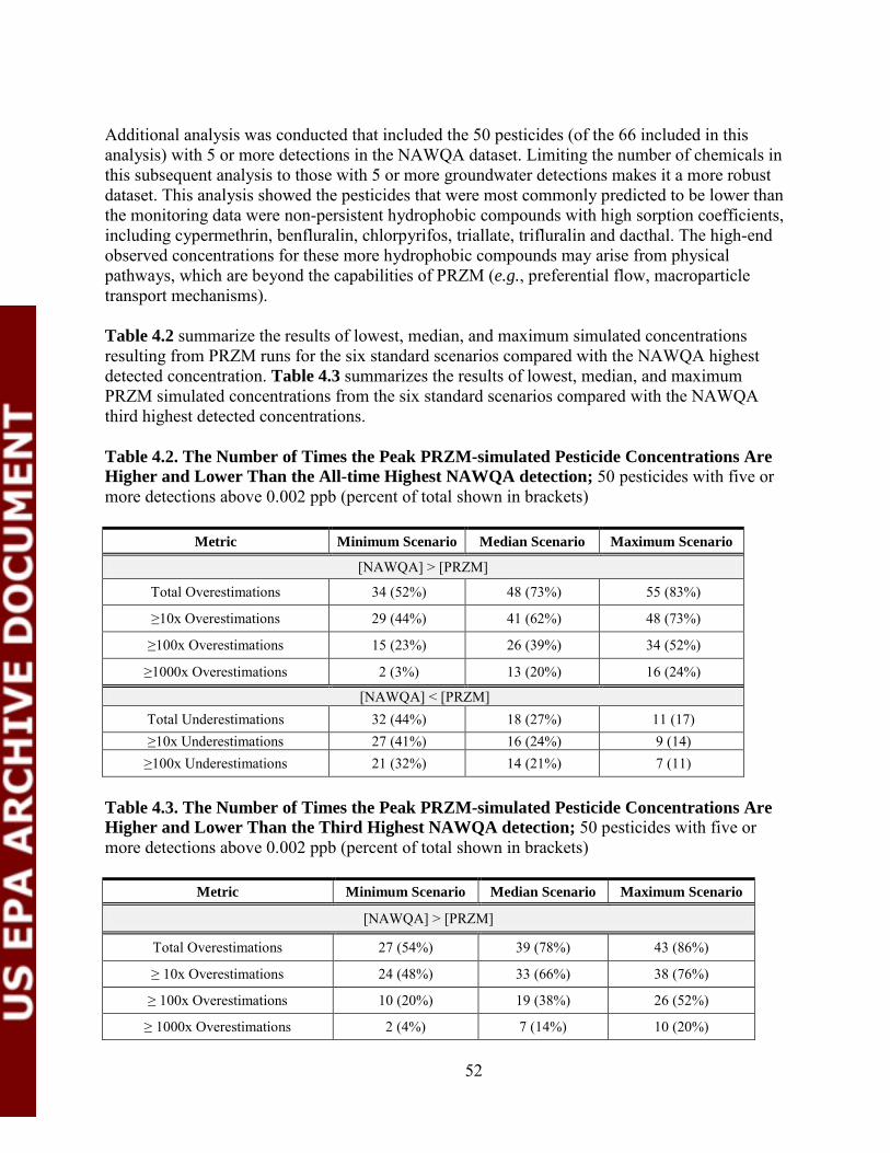
52

Additional analysis was conducted that included the 50 pesticides (of the 66 included in this analysis) with 5 or more detections in the NAWQA dataset. Limiting the number of chemicals in this subsequent analysis to those with 5 or more groundwater detections makes it a more robust dataset. This analysis showed the pesticides that were most commonly predicted to be lower than the monitoring data were non-persistent hydrophobic compounds with high sorption coefficients, including cypermethrin, benfluralin, chlorpyrifos, triallate, trifluralin and dacthal. The high-end observed concentrations for these more hydrophobic compounds may arise from physical pathways, which are beyond the capabilities of PRZM (e.g., preferential flow, macroparticle transport mechanisms). Table 4.2 summarize the results of lowest, median, and maximum simulated concentrations resulting from PRZM runs for the six standard scenarios compared with the NAWQA highest detected concentration. Table 4.3 summarizes the results of lowest, median, and maximum PRZM simulated concentrations from the six standard scenarios compared with the NAWQA third highest detected concentrations. Table 4.2. The Number of Times the Peak PRZM-simulated Pesticide Concentrations Are Higher and Lower Than the All-time Highest NAWQA detection; 50 pesticides with five or more detections above 0.002 ppb (percent of total shown in brackets)

Metric Minimum Scenario Median Scenario Maximum Scenario

[NAWQA] > [PRZM]

Total Overestimations 34 (52%) 48 (73%) 55 (83%)

≥10x Overestimations 29 (44%) 41 (62%) 48 (73%)

≥100x Overestimations 15 (23%) 26 (39%) 34 (52%)

≥1000x Overestimations 2 (3%) 13 (20%) 16 (24%)

[NAWQA] < [PRZM] Total Underestimations 32 (44%) 18 (27%) 11 (17) ≥10x Underestimations 27 (41%) 16 (24%) 9 (14)

≥100x Underestimations 21 (32%) 14 (21%) 7 (11)

Table 4.3. The Number of Times the Peak PRZM-simulated Pesticide Concentrations Are Higher and Lower Than the Third Highest NAWQA detection; 50 pesticides with five or more detections above 0.002 ppb (percent of total shown in brackets)

Metric Minimum Scenario Median Scenario Maximum Scenario

[NAWQA] > [PRZM]

Total Overestimations 27 (54%) 39 (78%) 43 (86%)

≥ 10x Overestimations 24 (48%) 33 (66%) 38 (76%)

≥ 100x Overestimations 10 (20%) 19 (38%) 26 (52%)

≥ 1000x Overestimations 2 (4%) 7 (14%) 10 (20%)

53

[NAWQA] < [PRZM]

Total Underestimations 23 (46%) 11 (22%) 7 (14%)

≥ 10x Underestimations 18 (36%) 10 (20%) 6 (12%)

≥ 100x Underestimations 13 (26%) 8 (16%) 4 (8%)

The maximum estimated PRZM concentration from all six standard scenarios minimizes the number of times that the observed concentration is greater than the estimated concentration; however, in general, the minimum estimated PRZM concentration from all six standard scenarios reduces the magnitude of the predicted concentrations that are greater than the observed concentrations. The purpose of this analysis is to employ PRZM as a screen, that is, to make sure that PRZM is not underestimating detected pesticide concentrations. The magnitude of overestimated value is less important and difficult to place in context since site specific information and pesticide use history are unknown. In summary, comparison of the NAWQA dataset with PRZM predicted pesticide concentrations indicate that PRZM can conservatively estimate pesticides concentrations for the majority of the chemicals evaluated. Nevertheless, some NAWQA detections are not captured by PRZM model estimates. PRZM was also observed to have a sufficiently protective buffer against underestimating (>100x) pesticide concentrations for some chemical detections reported in the NAWQA dataset. Therefore, based on this evaluation, PRZM meets the quality objectives by conservatively predicting the occurrence of pesticides in groundwater when conservative input assumptions are made for the majority of chemicals evaluated. An additional analysis comparing the PRZM-simulated concentration was completed and compared to the Human Health Benchmarks for Pesticides (HHBP). As shown in Table 4.5, for the majority of PRZM-estimated concentrations, there are about 20% that exceed the HHBP for acute and chronic endpoints. This analysis indicates that PRZM is not likely to be an overly burdensome screening-level tool for estimating pesticide concentrations. Table 4.4. Summary of the PRZM-GW Output with the Human Health Benchmarks for Pesticides

> Acute HHBP or HA

> Chronic (20% RSC)

HHBP

> Chronic (100% RSC)

HHBP Max >MCL?

TOTAL 10 18 12 5 % for chem with HHBP 19%1 35% 23% 71% % of all 66 chemicals 15% 27% 18% 7%

110 chemicals that have chronic HHBPs do not have an established acute HHBP because there were no frank effects observed. Relative Source Contribution (RSC)

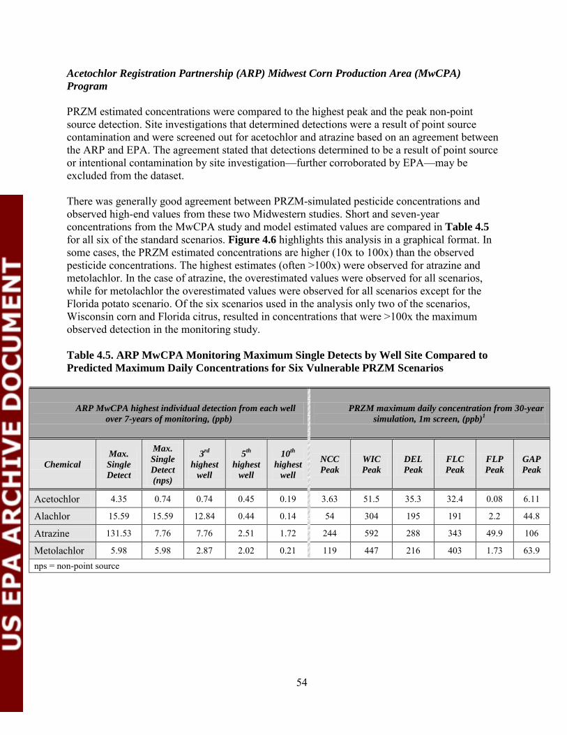
54

Acetochlor Registration Partnership (ARP) Midwest Corn Production Area (MwCPA) Program PRZM estimated concentrations were compared to the highest peak and the peak non-point source detection. Site investigations that determined detections were a result of point source contamination and were screened out for acetochlor and atrazine based on an agreement between the ARP and EPA. The agreement stated that detections determined to be a result of point source or intentional contamination by site investigation—further corroborated by EPA—may be excluded from the dataset. There was generally good agreement between PRZM-simulated pesticide concentrations and observed high-end values from these two Midwestern studies. Short and seven-year concentrations from the MwCPA study and model estimated values are compared in Table 4.5 for all six of the standard scenarios. Figure 4.6 highlights this analysis in a graphical format. In some cases, the PRZM estimated concentrations are higher (10x to 100x) than the observed pesticide concentrations. The highest estimates (often >100x) were observed for atrazine and metolachlor. In the case of atrazine, the overestimated values were observed for all scenarios, while for metolachlor the overestimated values were observed for all scenarios except for the Florida potato scenario. Of the six scenarios used in the analysis only two of the scenarios, Wisconsin corn and Florida citrus, resulted in concentrations that were >100x the maximum observed detection in the monitoring study. Table 4.5. ARP MwCPA Monitoring Maximum Single Detects by Well Site Compared to Predicted Maximum Daily Concentrations for Six Vulnerable PRZM Scenarios

ARP MwCPA highest individual detection from each well over 7-years of monitoring, (ppb)

PRZM maximum daily concentration from 30-year simulation, 1m screen, (ppb)1

Chemical Max. Single Detect

Max. Single Detect (nps)

3rd

highest well

5th highest

well

10th highest

well

NCC Peak

WIC Peak

DEL Peak

FLC Peak

FLP Peak

GAP Peak

Acetochlor 4.35 0.74 0.74 0.45 0.19 3.63 51.5 35.3 32.4 0.08 6.11

Alachlor 15.59 15.59 12.84 0.44 0.14 54 304 195 191 2.2 44.8

Atrazine 131.53 7.76 7.76 2.51 1.72 244 592 288 343 49.9 106

Metolachlor 5.98 5.98 2.87 2.02 0.21 119 447 216 403 1.73 63.9

nps = non-point source

55

Figure 4.6. ARP MwCPA Monitoring Maximum Single Detections Compared to Predicted Maximum PRZM-Simulated Concentrations The concentrations observed in the 3rd, 5th, and 10th highest monitored wells are provided in Table 4.5 to illustrate the potential variability between the wells. This is likely a reflection of the pesticide use history in the zone of influence as well as the difference in the vulnerability of each well. Additional (refined) modeling was completed to better represent the use intensity in the MwCPA study. The 30-year simulations were conducted using only seven years of maximum application applied every other year to match the study duration and the assumed crop rotation in the zone of influence. The Wisconsin corn scenario was used as a representative surrogate for the ARP MwCPA study site. The results are presented in Table 4.6 and Table 4.7. Table 4.6 shows that the highest PRZM estimated concentrations were similar but less than the maximum detected acetochlor concentration. Figure 4.6 compares this refined analysis with the initial screening- level simulation analysis. There is evidence to suggest the maximum detection is the result of a point source contamination for some of the chemicals (i.e., acetochlor and atrazine); therefore, a comparison of the modeling data with the highest non-point source detection may be more appropriate. PRZM estimates with modified use intensity are within the same order of magnitude as the maximum non-point source detection for acetochlor and alachlor, while the refined estimates are within two orders of magnitude of the atrazine and metolachlor detections.

56

Table 4.6. ARP MwCPA Monitoring Maximum Single Detects Compared to PRZM Predicted Concentrations with Refined Pesticide Application Events19

ARP MwCPA Highest Individual Detection From All Wells Over 7 Years of Monitoring (ppb)

PRZM Peak Daily Concentration for WIC Scenario (ppb)1

Chemical Max. Single Detect

Max. Single Detect (nps)

3rd

highest well

5th highest

well

10th highest

well

Initial Screen application

every year for 30 years

Refined Simulation

application every other year for 7

years

Acetochlor 4.35 0.74 0.74 0.45 0.19 51.5 4.3

Alachlor 15.59 15.59 12.84 0.44 0.14 304 118.8

Atrazine 131.53 7.76 7.76 2.51 1.72 592 287.5

Metolachlor 5.98 5.98 2.87 2.02 0.21 447 223.9 1Wisconsin Corn scenario was used to provide a more regionally representative scenario. nps = non-point source

Table 4.7. ARP MwCPA Monitoring Maximum Long-term (Seven years) Concentrations Compared to Refined Pesticide Application Events19

ARP MwCPA Detection From All Wells Over 7 Years of Monitoring (ppb)

PRZM Post-breakthrough

Average Concentration for

WIC Scenario (ppb)1

Time to Breakthrough (approx. years)

for WIC Scenario

Chemical Max.7-year Mean Concentration

Highest (nps)2

3rd

Highest 5th

Highest 10th

Highest Application Every Other Year

for 7 Years

Acetochlor 0.18 0.08 0.08 0.04 0.01 2.1 9.5

Alachlor 1.17 1.17 0.04 0.02 0.01 27.8 8.7

Atrazine 3.23 2.02 1.17 0.94 0.62 90.7 7.6

Metolachlor 1.48 1.48 0.35 0.16 0.03 83.9 11.5 1Wisconsin Corn scenario was used to provide a more regionally representative scenario. 2 Point source wells removed from analysis nps = non-point source

Analysis of the post breakthrough average concentration20 compared to the monitoring data indicates that model predictions are higher than the reported 7-year average (Table 4.7);

19 Refinements to pesticide application were made to better simulate applications that occurred in the study for acetochlor (every other year for seven years). 20 The average concentration of a pesticide in the aquifer after breakthrough is observed.

57

however, the simulated time to breakthrough21 indicates that breakthrough is expected beyond the study duration. In summary, the refined simulation results indicate that PRZM used as a screening tool (i.e., applications occur every year at maximum labeled rate for the duration of the simulation) produces conservative upper bound estimates of exposure in groundwater compared to targeted monitoring data. This analysis shows that when adjustments are made to the PRZM input values to better reflect the actual use, PRZM estimated pesticide concentrations compare well to the monitoring data. The simulated time to breakthrough for all chemicals is greater than the duration of the monitoring study. This result may suggest that the monitoring program may not have been long enough to capture the maximum levels of acetochlor in groundwater for the chemicals included in this analysis.

National Alachlor Well-Water Survey (NAWWS)

A comparison of the maximum observed pesticide concentrations in the NAWWS survey and the PRZM simulated pesticide concentration using two different scenarios, Wisconsin corn and North Carolina cotton, are provided in Table 4.8, 4.9, and 4.10. The results show that PRZM-estimated pesticide concentrations are greater than the observed NAWWS highest one-time sample. Wisconsin corn scenario produces substantially higher concentrations than the North Carolina cotton scenario. Two of three predicted PRZM pesticide concentrations at the North Carolina scenario are within the same order of magnitude of the highest detection in the NAWWS survey. Table 4.8. Comparison of NAWWS Alachlor Concentrations in Private Domestic Wells to PRZM Simulated Maximum Concentration (ppb)

Study ID. and Measurement Type for Alachlor Highest Detect 3rd Highest 5th Highest 95th %ile

NAWWS one-time sample 6.19 1.07 0.72 0.00 PRZM WIC peak, 30 years of application 304 PRZM NCC peak, 30 years of application 54

21 The time to breakthrough is the theoretical time that it takes for chemical to reach the aquifer following application.

58

Table 4.9. Comparison of NAWWS Atrazine Concentrations in Private Domestic Wells to PRZM Simulated Peak Concentration (ppb)

Study ID. and Measurement Type for Atrazine Highest Detect 3rd Highest 5th Highest 95th %ile

NAWWS one-time sample 6.72 1.96 1.02 0.05 PRZMGW WIC Peak, 100 years of application 592 PRZMGW NCC Peak, 100 years of application 44

Table 4.10. Comparison of NAWWS Metolachlor Concentrations in Private Domestic Wells to Simulated Peak Concentration (ppb)

Study ID. and Measurement Type for Metolachlor Highest Detect 3rd Highest 5th Highest 95th %ile

NAWWS one-time sample 3.81 1.60 0.51 0.00 PRZMGW WI, 100 years of application 447 PRZMGW NC Peak, 100 years of application 119

North Carolina PGW Study

Model runs were completed with a scenario that was developed specifically for the NC oxamyl study (i.e., the soil profile was parameterized with soil properties reported in the study report, and local weather data were used). During the early stages of analysis, superpositioning of peaks was observed to occur when model simulations were completed with applications occurring every year. The effect of superpositioning and the impact on groundwater concentrations was investigated. By simulating the frequency of applications once every 10 years, the year to year variability could be investigated without the interference of superpositioning of peaks. Figure 4.7 shows the time-series of simulated concentrations at the NC site where three different 10-year simulations were overlaid.

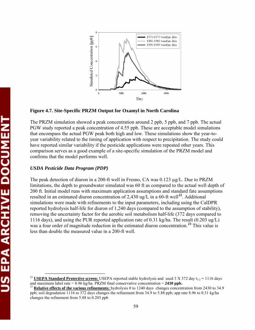
59

Figure 4.7. Site-Specific PRZM Output for Oxamyl in North Carolina The PRZM simulation showed a peak concentration around 2 ppb, 5 ppb, and 7 ppb. The actual PGW study reported a peak concentration of 4.55 ppb. These are acceptable model simulations that encompass the actual PGW peak both high and low. These simulations show the year-to- year variability related to the timing of application with respect to precipitation. The study could have reported similar variability if the pesticide applications were repeated other years. This comparison serves as a good example of a site-specific simulation of the PRZM model and confirms that the model performs well. USDA Pesticide Data Program (PDP) The peak detection of diuron in a 200-ft well in Fresno, CA was 0.123 µg/L. Due to PRZM limitations, the depth to groundwater simulated was 60 ft as compared to the actual well depth of 200 ft. Initial model runs with maximum application assumptions and standard fate assumptions resulted in an estimated diuron concentration of 2,430 ug/L in a 60-ft well22. Additional simulations were made with refinements to the input parameters, including using the CalDPR reported hydrolysis half-life for diuron of 1,240 days (compared to the assumption of stability), removing the uncertainty factor for the aerobic soil metabolism half-life (372 days compared to 1116 days), and using the PUR reported application rate of 0.31 kg/ha. The result (0.203 ug/L) was a four order of magnitude reduction in the estimated diuron concentration.23 This value is less than double the measured value in a 200-ft well.

22 USEPA Standard Protective screen: USEPA reported stable hydrolysis and used 3 X 372 day t1/2 = 1116 days and maximum label rate = 8.96 kg/ha. PRZM final conservative concentration = 2430 ppb. 23 Relative effects of the various refinements: hydrolysis 0 to 1240 days changes concentration from 2430 to 34.9 ppb; soil degradation 1116 to 372 days changes the refinement from 34.9 to 5.88 ppb; app rate 8.96 to 0.31 kg/ha changes the refinement from 5.88 to 0.203 ppb

60

Summary

Model Performance Summary

Comparison of targeted and non-targeted monitoring data with PRZM-predicted pesticide concentrations shows that when conservative input parameters (i.e., maximum application rates, annually repeated applications, half-life assumptions, or application methods) are used, PRZM produces upper bound estimates of exposure in groundwater for the majority of pesticides. Nevertheless, some of the detections in the monitoring data are not captured by PRZM model estimates. This outcome may be a result of processes not considered in PRZM such as preferential flow or macroparticle transport. Using conservative input parameters, PRZM conservatively estimates (>100x) pesticide concentrations for most chemicals; however, when site-specific adjustments are made, PRZM-estimated pesticide concentrations are close (with an order of magnitude) to observed data. This suggests that PRZM overestimation is due to use of conservative input parameters rather than to the conceptual groundwater model itself. Further, the comparison with the HHBP shows that exceedance of published benchmarks and subsequent risk concerns are relatively few and that approximately no more than 25% of chemical simulations will require simulation refinements. The comparison with targeted monitoring data shows that PRZM can also accurately estimate concentration if properly parameterized with site-specific data. This will allow for refined pesticide leaching analyses, including exploration of geographic, management, and usage refinements as well as opportunities to evaluate other mitigation options.

61

References NAWQA Program: Overall description of the NAWQA program: http://water.usgs.gov/nawqa/about.html Overview and links to key publications regarding pesticide monitoring under the NAWQA program: http://water.usgs.gov/nawqa/pnsp/ Summary reports related to the NAWQA groundwater monitoring: DeSimone, L.A., Hamilton, P.A., Gilliom, R.J., 2009, Quality of water from domestic wells in principal aquifers of the United States, 1991–2004—Overview of major findings: U.S. Geological Survey Circular 1332, 48 p. Gilliom, R. J. , J.E. Barbash, C.G. Crawford, P.A. Hamilton, J.D. Martin, N. Nakagaki, L.H. Nowell, J.C. Scott, P.E. Stackelberg, G.P. Thelin, and D.M. Wolock. 2006. Pesticides in the Nation’s Streams and Ground Water, 1992–2001. U.S. Geological Survey Circular 1291,172 p. Toccalino, P.L., and Hopple, J.A., 2010, The quality of our Nation’s waters—Quality of water from public-supply wells in the United States, 1993–2007—Overview of major findings: U.S. Geological Survey Circular 1346, 58 p. Data used in this study is stored at the following location: water.usgs.gov/nawqa/data Details of data retrieval: # METADATA Date: May 21, 2010 # Filename: EPA.GW.QW.DATA.rdb Includes all data for pesticides in filtered ground-water samples # These data were retrieved from the USGS NAWQA Data Warehouse in September 2006 and # reviewed by Jeffrey D. Martin (U.S. Geological Survey NAWQA Pesticide Synthesis Project; email: jdmartin@usgs.gov ). NAWWS Study: Holden, L.R., J.A. Graham, R.W. Whitmore, W. J.. Alexander, R.W. Pratt, S.K. Liddle, L.L. Piper. 1992. Results of the National Alachlor Well Water Survey. Environmental Science & Technology 26 (5), 935-943.

Liddle, S. K., R. W. Whitmore, R. E. Mason, W. J. Alexander, and L. R. Holden. 1990. Accounting for temporal variations in large-scale retrospective studies of agricultural chemicals in ground water. Ground Water Monitoring Review. Winter, pp. 142-145.

62

Holden, L.R., R.W. Whitmore, and l.A. Graham. 1988. The national alachlor well water survey: Statistical design and current status. In Proceedings of the Agricultural Impacts on Ground Water Conference, National Water Well Assoc. Des Moines, Iowa. pp. 237-254.

ARP MwCPA Study: MRID: 43899601 Hendley, P. (1995) State Ground Water Monitoring Program for Acetochlor and Other Corn Herbicides--Part 1: Site Selection and Site Details: Lab Project Number: ACET-94-GW-01: RR 95-087B: GWMSIT05.DOC. Unpublished study prepared by Zeneca Ag Products and Levine-Fricke, Inc. 3217 p.

MRID: Not Assigned. Hendley, P. (1996) State Ground Water Monitoring Program for Acetochlor and Other Corn Herbicides--Part 2. 1995 Progress Report: Lab Project Number: Zeneca #ACET-95-GW-02; Levine-Fricke #3276.101; Report #RR 96-019B. Unpublished study prepared by Zeneca Ag Products; Monsanto; Levine, Fricke. 261 p.

MRID: 44422501 Hendley, P. (1997) State Ground Water Monitoring Program for Acetochlor and Other Corn Herbicides--Part 3. 1996 Progress Report: Lab Project Number: ACET-95-GW-02: 3276.101: RR 97-034B. Unpublished study prepared by Zeneca Ag Products; Monsanto; Levine, Fricke, Recon Inc. 138 p. OPP DP Barcode D252465.

MRID: 44599201 Hendley, P. (1998) State Ground Water Monitoring Program for Acetochlor and other Corn Herbicides--Part 4. 1997 Progress Report: Lab Project Number: RR 98-026B: ACET-95-GW-02: 3276. 101. Unpublished study prepared by Zeneca Ag Products and Monsanto. 137 p.

MRID: 44948701 De Guzman, N. (1999) State Groundwater Monitoring Program for Acetochlor and Other Corn Herbicides--Part 5: 1998 Progress Report: Lab Project Number: ACET-95-GW-02: 3276.101: RR 99-031B. Unpublished study prepared by Zeneca Ag Products; Monsanto and LFR Levine-Fricke. 143 p.

MRID: 45208501 De Guzman, N. (2000) State Ground Water Monitoring Program for Acetochlor and Other Corn Herbicides-Part 6: Lab Project Number: ACET-95-GW-02: 3276.101: RR 00-100B. Unpublished study prepared by Levine-Fricke, Zeneca, and Alta Analytical Laboratory, Inc. 191 p.

MRID: 45449601 De Guzman, N. (2001) State Ground Water Monitoring Program for Acetochlor and Other Corn Herbicides--Part 7: 2000 Progress Report: Lab Project Number: 852-562: ACET-95-GW-02:

63

3276.101. Unpublished study prepared by LFR Levine-Fricke, Monsanto, and Dow AgroSciences LLC. 15 p.

MRID: 45722701 de Guzman, N.; Fuhrman, J.; Gustafson, D.; et al. (2002) State Ground Water Monitoring Program For Acetochlor and Other Corn Herbicides--Part 8. 2001 Progress Report: Lab Project Number: ACET-95-GW-02: 3276.101: ARP-GWM-01. Unpublished study prepared by LFR Levine Fricke (LFR), Dow AgroSciences LLC and Monsanto. 158 p.

MRID: 45728401 van Wesenbeeck, I.; De Guzman, N.; Fuhrman, J.; et al. (2002) State Ground Water Monitoring Program for Acetochlor and Other Corn Herbicides--Part 9: Final Study Report: Lab Project Number: ARP-GWM-02: 852-577: ACET-95-GW-02. Unpublished study prepared by LFR Levine-Fricke and Monsanto. 121 p.

MRID: 45730201 De Guzman, N.; Wesenbeeck, I. (2002) State Ground Water Monitoring Program for Acetochlor and Other Corn Herbicides--Part 10 Amendment to the Final Study Report: Lab Project Number: ACET-94-GW-01: 3276.101: 852-578. Unpublished study prepared by LFR Levine Fricke, Monsanto and Dow AgroSciences LLC. 300 p.

Oxamyl PGW Field Study: MRID: 45591605 Hiscock, A. M., R. L. Warren, and B. Patterson. 2002. A Small-Scale Prospective Groundwater Monitoring Study for Oxamyl. DuPont Report No. AMR 4318-97. Unpublished study conducted by Stone Environmental, Inc., Raleigh, NC; Ecologic, Inc., Hurdle Mills, NC; Agricultural Systems Associates, Cary, NC; AGVISE Laboratories, Benson, MI; Centre Analytical Laboratories, Inc., State College, PA; and E.I. du Pont de Nemours and Company, Wilmington, DE.; submitted by E.I. du Pont de Nemours and Company, Wilmington, DE. Jan. 14, 2002. 242 p. PDP Field Studies and CPUR Data: http://www.ams.usda.gov/AMSv1.0/ams.fetchTemplateData.do?template=TemplateC&navID=&rightNav1=&topNav=&leftNav=ScienceandLaboratories&page=PesticideDataProgram&resultType=&acct=pestcddataprg http://www.cdpr.ca.gov/docs/pur/purmain.htm

64

Chapter 5: REPORT CONCLUSIONS

Canada and the United States combined efforts as part of the North American Free Trade Agreement (NAFTA) to develop a harmonized groundwater modeling protocol. This included the development of a common conceptual groundwater modeling scenario for regulatory purposes designed to be protective of even the most vulnerable drinking water supplies. Nineteen existing modeling programs were screened as candidate programs to implement the conceptual model. Of the 19 modeling programs screened, three were selected for further evaluation including the Pesticide Root Zone Model (PRZM), the Pesticide Emission Assessment at Regional and Local Scales (PEARL), and Leaching Estimation and Chemistry Model – Pesticides (LEACHM). The three finalist models were evaluated for their ability to accurately simulate water flow, pesticide concentrations, and soil temperature relative to field data. All three modeling programs performed adequately and could be applied as a tool to simulate pesticide transport to groundwater. PRZM was selected as the NAFTA regulatory tool to implement the conceptual model because of ease of use and in-house expertise required for maintenance. PRZM was further evaluated by comparing simulated pesticide concentrations to targeted and non-targeted monitoring data. For the majority of chemicals tested, PRZM-predicted pesticide concentrations represented conservative upper bound estimates of exposure in groundwater when conservative input parameters (i.e., maximum application rates, annually repeated applications, half-life assumptions, or application methods) are used. Nevertheless, there are some pesticide detections in monitoring data that are not captured by PRZM model estimates. This may be a result of processes such as preferential flow or macroparticle transport that are not accounted for in the conceptual model implemented in PRZM. With site specific adjustments to the PRZM input values estimated pesticide concentrations compare well to monitoring data (within a factor of 10). The evaluation demonstrates that PRZM is a versatile risk assessment tool that can be used both as a screening tool and a refined site-specific tool in risk assessment. Based on the analysis in the previous chapters, PRZM is an effective tool to produce upper bound pesticide concentrations in groundwater for national as well as site-specific assessments. Additionally, while Canada has previously identified scenarios representative of major agricultural areas across the country, it is well-documented that a few relatively rare regions have exceptionally vulnerable groundwater (primarily the Florida’s Central Ridge, Wisconsin Central Sands and Long Island, New York areas) where the level of pesticide contamination for more mobile and persistent compounds can be significantly higher than the rest of the United States. This fact is reflected in both the monitoring data and the model estimates. This needs to be considered in developing a screening process for drinking water where the pesticide use areas may or may not include parts of such areas with drinking water wells completed in highly vulnerable aquifers. Based upon this analysis, the team recommends the following be considered for further improvements to simulating groundwater concentrations with PRZM:

• Investigation of low-level microbial degradation or other dissipation processes in subsoil horizons and potential impacts on simulated concentrations in groundwater.

65

• An evaluation of hydrolysis rates and variation with pH and temperature and the model sensitivity to these inputs.

• Use of a hydrolysis degradation rate where the rate of degradation is significantly different from zero for routine modeling applications.

• Additional evaluation of detections observed in monitoring data that are significantly below model estimates and the impact this may have on human health risk assessment.

• Additional evaluation of the effect well screen length has on the predicted concentration in groundwater.

66

APPENDIX A

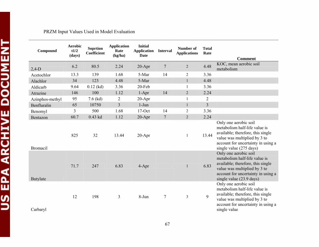
67

PRZM Input Values Used in Model Evaluation

Compound Aerobic

t1/2 (days)

Soprtion Coefficient

Application Rate

(kg/ha)

Initial Application

Date Interval Number of

Applications Total Rate

Comment

2,4-D 6.2 80.5 2.24 20-Apr 7 2 4.48 KOC, mean aerobic soil metabolism

Acetochlor 13.3 139 1.68 5-Mar 14 2 3.36 Alachlor 34 123 4.48 5-Mar 1 4.48

Aldicarb 9.64 0.12 (kd) 3.36 20-Feb 1 3.36 Atrazine 146 100 1.12 1-Apr 14 2 2.24

Azinphos-methyl 95 7.6 (kd) 2 20-Apr 1 2 Benfluralin 65 10750 3 1-Jun 1 3

Benomyl 3 500 1.68 17-Oct 14 2 3.36 Bentazon 60.7 0.43 kd 1.12 20-Apr 7 2 2.24

Bromacil

825 32 13.44 20-Apr 1 13.44

Only one aerobic soil metabolism half-life value is available; therefore, this single value was multiplied by 3 to account for uncertainty in using a single value (275 days)

Butylate

71.7 247 6.83 4-Apr 1 6.83

Only one aerobic soil metabolism half-life value is available; therefore, this single value was multiplied by 3 to account for uncertainty in using a single value (23.9 days)

Carbaryl

12 198 3 8-Jun 7 3 9

Only one aerobic soil metabolism half-life value is available; therefore, this single value was multiplied by 3 to account for uncertainty in using a single value

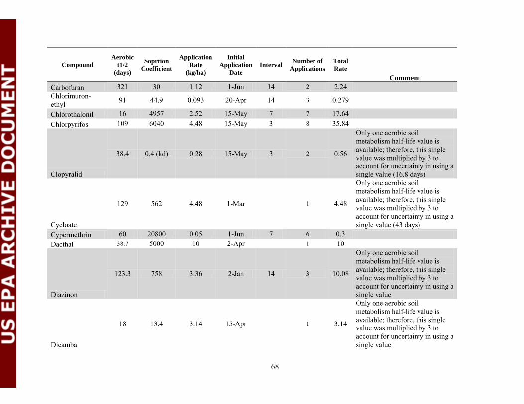
68

Compound Aerobic

t1/2 (days)

Soprtion Coefficient

Application Rate

(kg/ha)

Initial Application

Date Interval Number of

Applications Total Rate

Comment Carbofuran 321 30 1.12 1-Jun 14 2 2.24 Chlorimuron-ethyl 91 44.9 0.093 20-Apr 14 3 0.279

Chlorothalonil 16 4957 2.52 15-May 7 7 17.64 Chlorpyrifos 109 6040 4.48 15-May 3 8 35.84

Clopyralid

38.4 0.4 (kd) 0.28 15-May 3 2 0.56

Only one aerobic soil metabolism half-life value is available; therefore, this single value was multiplied by 3 to account for uncertainty in using a single value (16.8 days)

Cycloate

129 562 4.48 1-Mar 1 4.48

Only one aerobic soil metabolism half-life value is available; therefore, this single value was multiplied by 3 to account for uncertainty in using a single value (43 days)

Cypermethrin 60 20800 0.05 1-Jun 7 6 0.3 Dacthal 38.7 5000 10 2-Apr 1 10

Diazinon

123.3 758 3.36 2-Jan 14 3 10.08

Only one aerobic soil metabolism half-life value is available; therefore, this single value was multiplied by 3 to account for uncertainty in using a single value

Dicamba

18 13.4 3.14 15-Apr 1 3.14

Only one aerobic soil metabolism half-life value is available; therefore, this single value was multiplied by 3 to account for uncertainty in using a single value

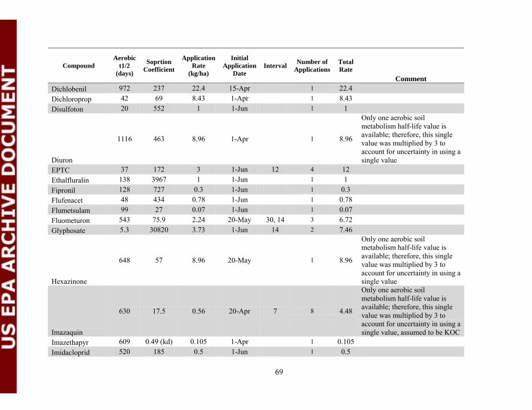
69

Compound Aerobic

t1/2 (days)

Soprtion Coefficient

Application Rate

(kg/ha)

Initial Application

Date Interval Number of

Applications Total Rate

Comment Dichlobenil 972 237 22.4 15-Apr 1 22.4 Dichloroprop 42 69 8.43 1-Apr 1 8.43

Disulfoton 20 552 1 1-Jun 1 1

Diuron

1116 463 8.96 1-Apr 1 8.96

Only one aerobic soil metabolism half-life value is available; therefore, this single value was multiplied by 3 to account for uncertainty in using a single value

EPTC 37 172 3 1-Jun 12 4 12 Ethalfluralin 138 3967 1 1-Jun 1 1

Fipronil 128 727 0.3 1-Jun 1 0.3 Flufenacet 48 434 0.78 1-Jun 1 0.78

Flumetsulam 99 27 0.07 1-Jun 1 0.07 Fluometuron 543 75.9 2.24 20-May 30, 14 3 6.72

Glyphosate 5.3 30820 3.73 1-Jun 14 2 7.46

Hexazinone

648 57 8.96 20-May 1 8.96

Only one aerobic soil metabolism half-life value is available; therefore, this single value was multiplied by 3 to account for uncertainty in using a single value

Imazaquin

630 17.5 0.56 20-Apr 7 8 4.48

Only one aerobic soil metabolism half-life value is available; therefore, this single value was multiplied by 3 to account for uncertainty in using a single value, assumed to be KOC

Imazethapyr 609 0.49 (kd) 0.105 1-Apr 1 0.105 Imidacloprid 520 185 0.5 1-Jun 1 0.5

70

Compound Aerobic

t1/2 (days)

Soprtion Coefficient

Application Rate

(kg/ha)

Initial Application

Date Interval Number of

Applications Total Rate

Comment Iprodione 48 426 4 1-Jun 14 6 24 PV included unextracted residues Isofenphos 352 972 2 1-Jun 14 2 4

Lindane

2940 1368 0.13 1-Apr 1 0.13

Only one aerobic soil metabolism half-life value is available; therefore, this single value was multiplied by 3 to account for uncertainty in using a single value

Linuron 213 2000 1.68 1-Apr 1 1.68 Malathion 3 151 7.84 1-Apr 1 7.84

Metalaxyl 419 409 4.48 1-Apr 3 3 13.44 Metolachlor 49 181 4.48 1-May 14 2 8.96

Metribuzin 318 32 6 20-Apr 1 6 assumed to be KOC Metsulfuron-methyl 31 7.7 0.028 1-Jun 14 2 0.056

Molinate 27 255 3 1-Jun 14 3 9 Myclobutanil 251 224 0.28 1-Jun 14 8 2.24

Napropamide 1338 577 4 20-Apr 1 4

Norflurazon

390 0.14 (kf) 8.96 1-Aug 1 8.96

Only one aerobic soil metabolism half-life value is available; therefore, this single value was multiplied by 3 to account for uncertainty in using a single value

Oryzalin

189 941 6.72 1-Apr 75 2 13.44

Only one aerobic soil metabolism half-life value is available; therefore, this single value was multiplied by 3 to account for uncertainty in using a single value

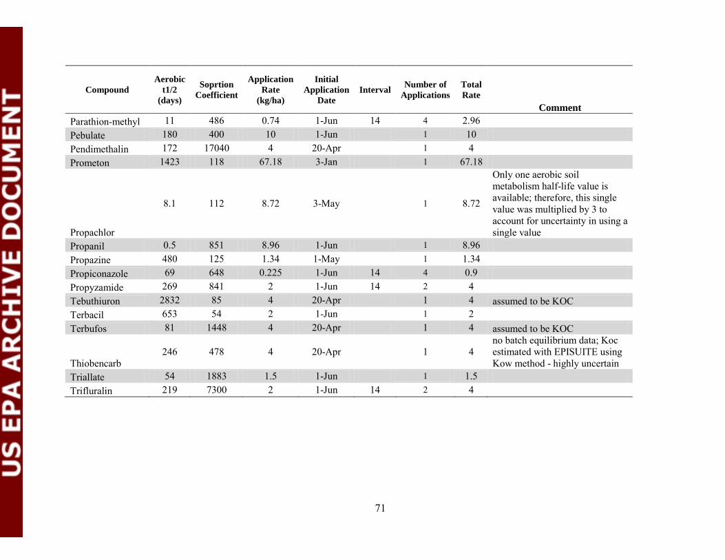
71

Compound Aerobic

t1/2 (days)

Soprtion Coefficient

Application Rate

(kg/ha)

Initial Application

Date Interval Number of

Applications Total Rate

Comment Parathion-methyl 11 486 0.74 1-Jun 14 4 2.96

Pebulate 180 400 10 1-Jun 1 10 Pendimethalin 172 17040 4 20-Apr 1 4

Prometon 1423 118 67.18 3-Jan 1 67.18

Propachlor

8.1 112 8.72 3-May 1 8.72

Only one aerobic soil metabolism half-life value is available; therefore, this single value was multiplied by 3 to account for uncertainty in using a single value

Propanil 0.5 851 8.96 1-Jun 1 8.96 Propazine 480 125 1.34 1-May 1 1.34

Propiconazole 69 648 0.225 1-Jun 14 4 0.9 Propyzamide 269 841 2 1-Jun 14 2 4

Tebuthiuron 2832 85 4 20-Apr 1 4 assumed to be KOC Terbacil 653 54 2 1-Jun 1 2

Terbufos 81 1448 4 20-Apr 1 4 assumed to be KOC

Thiobencarb 246 478 4 20-Apr 1 4

no batch equilibrium data; Koc estimated with EPISUITE using Kow method - highly uncertain

Triallate 54 1883 1.5 1-Jun 1 1.5 Trifluralin 219 7300 2 1-Jun 14 2 4