
MA/MSc MT-03
Vardhaman Mahaveer Open University, Kota
Differential Equations, Calculus of Variationsand Special Functions

Course Development CommitteeChairmanProf. (Dr.) Naresh DadhichVice-ChancellorVardhaman Mahaveer Open University, Kota
Co-ordinator/Convener and MembersSubject Convener Co-ordinatorProf. D.S. Chauhan Dr. Anuradha SharmaDepartment of Mathematics Assistant ProfessorUniversity of Rajasthan, Jaipur Department of Botany, V.M.O.U., KotaMembers :
1. Prof. V.P. Saxena 4. Prof. S.P. Goyal 7. Dr. Paresh VyasEx Vice-Chancellor Emeritus Scientist (CSIR) Assistant ProfessorJiwaji University, Deptt. of Mathematics Deptt. of MathematicsGwalior (MP) University of Rajasthan, Jaipur University of Rajasthan, Jaipur
2. Prof. S.C. Rajvanshi 5. Dr. A.K. Mathur 8. Dr. Vimlesh SoniDeptt. of Mathematics Associate Prof. (Retired) LecturerInstitute of Eng. & Tech. Deptt. of Mathematics Deptt. of MathematicsBhaddal, Ropar (Punjab) University of Rajasthan, Jaipur Govt. PG College, Kota (Raj.)
3. Prof. P.K. Banerjee 6. Dr. K.N. Singh 9. Dr. K.K. MishraEmeritus Fellow (UGC) Associate Prof. (Retired) LecturerDeptt. of Mathematics Deptt. of Mathematics Deptt. of MathematicsJ.N.V. University, Jodhpur University of Rajasthan, Jaipur M.S.J. Collage, Bharatpur (Raj.)
10. Dr. K.S. ShekhawatLecturer, Deptt. of MathematicsGovt. Shri Kalyan College, Sikar (Raj.)
Editing and Course WritingEditor WritersProf. S.P. Goyal 1. Prof. Kantesh Gupta 2. Dr. Atul GargEmeritus Scientist (CSIR) Deptt. of Mathematics Lecturer, Deptt. of MathematicsDeptt. of Mathematics MNIT, Jaipur Seth Moti Lal PG College, JhunjhunuUniversity of Rajasthan, Jaipur 3. Dr. K.S. Shekhawat 4. Dr. Chandra Shekhar
Lecturer, Deptt. of Mathematics Assistant ProfessorGovt. Sri Kalyan College, Sikar Mathematics Group
5. Mr. Pranay Goswamy Birla Institute of TechnologyLecturer, Deptt. of Mathematics and Science, PilaniAmity University, Jaipur
Academic and Administrative Management
Course Material Production Mr. Yogendra Goyal Assistant Production Officer Vardhaman Mahaveer Open University, Kota
Prof. (Dr.) Naresh DadhichVice-Chancellor
Vardhaman Mahveer Open University, Kota
Prof. M.K. Ghadoliya Director (Academic)
Vardhaman Mahveer Open University, Kota
Mr. Yogendra Goyal Incharge
Material Production andDistribution Department

MA/MSc MT-03
Vardhaman Mahaveer Open University, Kota
Differential Equations, Calculus of Variations and Special Functions
Unit No. Units Page No.
1. Non-Linear Ordinary Differential Equations of Particular
Forms and Riccati’s Equation 1–24
2. Total Differential Equations 25–45
3. Partial Differential Equations of Second order, Monge’s Method 46–64
4. Classification of Linear PDE of Second Order, Cauchy Problem and
Method of Separation of Variables 65–80
5. Laplace, Wave and Diffusion Equations And Canonical Forms 81–100
6. Eigenvalues, Eigenfunctions and Sturm-Liouville
Boundary Value Probleon 101–120
7. Variational Problems with Fixed Boundaries and
Euler-Lagrange Equation 121–138
8. Functionals Dependent on Higher Order Derivatives and
Variational Problems in Parametric Form 139–156
9. Series Solution of Second Order Linear Differential Equation 157–181
10. Gauss Hypergeometric Function: its Properties and
Integral Representation 182–200
11. Gauss and Confluent Hypergeometric Functions 201–217
12. Legendre’s Polynomials and Functions Pn(x) and Qn (x) 218–246
13. Bessel’s Functions 247–268
14. Hermite Polynomials 269–285
15. Laguerre Polynomials 286–303
Reference Books 304

PREFACE
The Present book entitled ‘‘Differential Equations, Calculus of Variations
and Special Functions’’ has been designed so as to cover the unit-wise syllabus of
Mathematics-Third paper for M.A./M.Sc. (Previous) students of Vardhaman
Mahaveer Open University, Kota. It can also be used for competitive examinations.
The basic principles and theory have been explained in a simple, concise and lucid
manner. Adequate number of illustrative examples and exercises have also been
included to enable the students to grasp the subject easily. The units have been
written by various experts in the field. The unit writers have consulted various
standard books on the subject and they are thankful to the authors of these refer-
ence books.
1
Unit 1 : Non-Linear Ordinary Differential Equations ofParticular Forms and Riccati’s Equation
Structure of the Unit
1.0 Objective
1.1 Introduction
1.2 Exact Non-Linear Differential Equation
1.3 Riccati’s Equation
1.3.1 General solution of Riccati’s equation
1.3.2 Theorem
1.3.3 Method of solution of Riccati’s equation when one particular solution is known
1.3.4 Method of solution of Riccati’s equation when two particular solutions are known
1.3.5 Method of solution of Riccati’s equation when three particular solutions are known
1.4 Equation of the form 2
2d y f ydx
1.5 Equations not containing y directly
1.6 Equation not containing x directly
1.7 Equations in which y appears in only two derivatives whose orders differ by two
1.8 Equations in which y appears in only two derivatives whose orders differ by unity
1.9 Homogeneous Equation
1.10 Summary
1.11 Answers of Self-Learning Exercise
1.12 Exercise
1.0 Objective
The purpose of this unit is to discuss various methods for solving some particular forms of sec-ond and higher order non-linear differential equations. The methods for solving exact non-linear differen-tial equations and Riccati’s equation are also discussed.

2
1.1 Introduction
In earlier classes we studied a great deal about linear differential equations of second and higherorders when coefficient may or may not be constant. It is a known fact that due to superimposition oflinearly independent solutions, it is easy to solve linear differential equation and we have well establishedtheories for such types of equations.
On the other hand, the non-linear differential equations are difficult to handle. In the case of some
first order equations, we have well established methods. However, there is no known general method
for solving second and higher order non linear differential equations. It is only some particular forms that
may be reduced to linear equations by suitable transformation and integrated to yield compact results.
The aim of this unit is to study those easily integrable non-linear equations.
Next we shall discuss the general solution of Riccati’s equation. The solution of this equation
when one, two or three particular solutions are known will also be discussed.
1.2 Exact Non-linear Differential Equations
There is no simple method for testing the exactness of non-linear differential equations as in the
case of linear equations. One possible method is that if the terms of the equation be grouped, by inspec-
tion, in such a way that they become perfect differential and their integrals may be written directly. The
other method of obtaining the integral of an exact differential equation, which is applicable both for linear
and non-linear equations is explained below.Let s = f (x) be a differential equation of nth order. If it is an exact deferential equation it should
be derived merely by differentiation, so as to contain n
nd ydx
in the first degree. Now we write the equa-
tion in the form sdx = f (x) dx and will integrates assuming that as if 1
1
n
nddx
y
were the only variable in the
differential equation and n
nd ydx
is its differential coefficient.
Denoting the result by s1 then sdx – ds1 will contain differential coefficients at the most upto
(n – 1 )th order. Restriction of taking 1
1
n
nddx
y
as the only variable should be removed while finding ds1.
Repeating the above process as many times as necessary, we shall finally getsdx – ds1 – ds2 – ... = 0
or ds1 + ds2 + ... = sdxOn integration, we get
s1 + s2 ... = sdx = f (x) dx
3
Ex.1. Show that the differential equation
3 22 23 2 2 0dy dy dy d yy + x + y + x + y =
dx dx dx dx
is an exact equation and find its first integral.Sol. The given equation can be written as
32 22 2
2 22 2 3 0d y dy d y dy dysdx x y y x y dxdx dx dxdx dx
Now here the first three terms are the differentiation of2
2 2dy dyx ydx dx
So putting2
2 21
dy dys x ydx dx
On differentiation, we get32 2
2 21 2 22 2 2
d y dy dy dy d yds x x y y dxdx dx dxdx dx
Thus 1dysdx ds y x dxdx
.....(1)
Again the terms on R.H.S. are the differentiation of xy, so puttings2 = xy
On differentiation, we get
2dyds x y dxdx
.....(2)
From (1) and (2), we finally getsdx – ds1 – ds2 = 0
which on integration givess1 + s2 = constant
This relation shows that the given equation is exact and the first integral will be given by2
2 2 .dy dyx y xy cdx dx
Ex.2. Solve the following differential equation :2
22sin 2cos 2sin 2 cos cos d y dy dyx + x + x + y x = xdx dxdx
Sol. We can writte the given equation as
2
22sin 2 cos 2sin 2 cos cosd y dy dysdx x x x y x dx x dxdx dxdx
4
Here first term of above equation will arise from the differentiation of 2sin dyxdx , so putting
1 2sin dys xdx
which implies that2
1 22sin 2cosd y dyds x x dxdxdx
Thus 1 2sin 2 cosdysdx ds x y x dxdx
Again putting
s2 = 2y sin xOn differentiation, we get
2 2sin 2 cosdyds x y x dxdx
sdx – ds1 – ds2 = 0This shows that the given equation is exact and on integrating, we get
s1 + s2 = sdx = cos x dx
or 1n2sin 2 sin si 2dyx y x x cdx
or 1 c1 cose2
dy y c xdx
This is a linear differential equation of first order whose integrating factor (I.F.) is ex
Thus its solution is
1 21. . . cosec . .2
y I F c x I F dx c
or 1 21 cosec2
x x xy e e c e x dx c
Ex.3. Solve
22
2 222 cos 2 sin cos sind y dy dyx y x y + x y y = log x
dx dxdxSol. The given equation is
222 2
22 cos 2 sin cos sin logd y dy dysdx x y x y x y y dx x dxdx dxdx
.....(3)
Let 21 2 cos dys x y
dx
So that2
2 21 22 cos 2 sin 4 cosd y dy dyds x y x y x y dx
dx dxdx

5
1 3 cos sin dysdx ds x y y dxdx
Again let s2 = – 3x sin y
So that 2 3 cos 3sin dyds x y y dxdx
s dx – ds1 – ds2 = 2sin y dxHence the equation is not exact.So dividing the given equation (3) by x2, we get
22
2 2 21 1 log2cos 2sin cos sind y dy dy xsdx y y y y dx dx
dx x dxdx x x
Now let 1 2cos dys ydx
so that22
1 2cos 2sind y dyds y y dxdx dx
1 21 1cos sindysdx ds y y dxx dx x
Again let 21 sins yx
So that 2 21 1cos sindyds y y dxx dx x
sdx – ds1 – ds2 = 0Hence the equation is exact, and
1 2 2log xds ds sdx dx
x
Integrating we get
1 2 121 logs s x dx cx
11 12cos sin log 1dyy y x c
dx x x .....(4)
Let sin y = u. Then
cos dy duydx dx
(4) reduces to
11 log 12 2 2
cdu u xdx x x
.....(5)
6
which is linear with1 12. .
dxxI F e x
Hence the solution of (5) is
12
log 112 2
x x cu x dx x dx cx
or 2 3 212
1sin 12 3
w cx y w e dw x c , where w = log x
2 2 3 2121 2
3w w cw e e x c
3 212log 1 2
3cx x x x c
or 1 212sin log 1
3cy x x c x
which is the required solution.
Ex.4. Solve22
22 0d y dyx y x y
dxdx
Sol. The given equation is22
2 2 22 2 0d y dy dysdx x y x xy y dx
dx dx dx
.....(6)
Let 21
dys x ydx
22
2 21 2 2d y dy dyds x y x xy dx
dx dx dx
So that 21 4 dysdx ds xy y dx
dx
Again let s2 = – 2xy2
So that 22 4 2dyds xy y dx
dx
sdx – ds1 – ds2 = 3y2 dxHence the equation is not exact.Therefore dividing the given equation (6) by x2, we get
22 2
2 2
2 0d y dy y dy ysdx y dxdx dx x dx x
Now let 1dys ydx

7
Then22
1 2
d y dyds y dxdx dx
So that2
1 2
2y dy ysdx ds dxx dx x
Let2 2
2 2 2
2so thaty y dy ys ds dxx x dx x
Hence sdx – ds1 – ds2 = 0or ds1 + ds2 = sdx = 0or s1 + s2 = c1
or2
1 dy yy cdx x
.....(7)
Let2
so that2y dy duu y
dx dx
Hence equation (7) becomes
12du u c
dx x .....(8)
which is linear with 2
2
1. .x dx
I F ex
Thus solution of (8) is
2
12 1 22 or
2cu yc x c c x
x x
or y2 = x(Ax – B),where A and B are arlitrary corstants.
1.3 Riccati’s Equation
Originally, the name Riccati’s equation was given to the differential equation
2 mdy by cxdx
.....(1)
where b are c are constants. Equation (1) can be written in the formy1 + by2 = cxm .....(2)
where suffixes denotes differentiation w.r.t. xThe more general form of (2) is
xy1 – ay + by2 = cxm .....(3)which can be easily reduced to the form
22 m adu b cu zdt a a
.....(4)
by using the substitution t = xa and then changing the variable y to u by substitution y = ut.

8
The Equation (4) can be easily written in the formy1 = P + Qy + Ry2 .....(5)
where P, Q and R are function of x.The equation (5) is known as the generalised Riccati’s equation.French Mathematician Liouville, in 1841, proved that equation (5) is one of the simplest differ-
ential equation of the first order and first degree that can not, in general be integrated by quadratures.Due to historical and theoretical importance and its usefulness in Differential Geometry, the study of Riccati’sequation becomes quite useful.
1.3.1 General solution of Riccati’s equation
Equation (5) can be reduced to a second order linear differential equation by introducing an-other dependent variable S such that
111
Sy S RSRS
.....(6)
On differentiation, we gety1 = – S2(RS)–1 + S1(RS)–2 [R1S + RS1] .....(7)
where a subscript denote differentiation with respect to x.Substituting (6) and (7) in (5), we get
2 22 1 1 1 1 1
2 2 2 2
S R S S S SP Q RRS R S RS RS R S
or –RS2 + R1S1 = PR2S – QS1Ror RS2 –(QR + R1) S1 + PR2S = 0 .....(8)This is linear differential equation of second order. We know that the general solution of (8) is of
the formS = Af (x) + Bg(x) .....(9)
where A and B are arbitrary constants and f (x), g(x) are two linearly independent integrals.Now, from (6) and (9), we get
1 1 1 1//
Af Bg A B f gy
R Af Bg R A B f g
which is of the form
1 1cf x g xy
R cf x g x
.....(10)
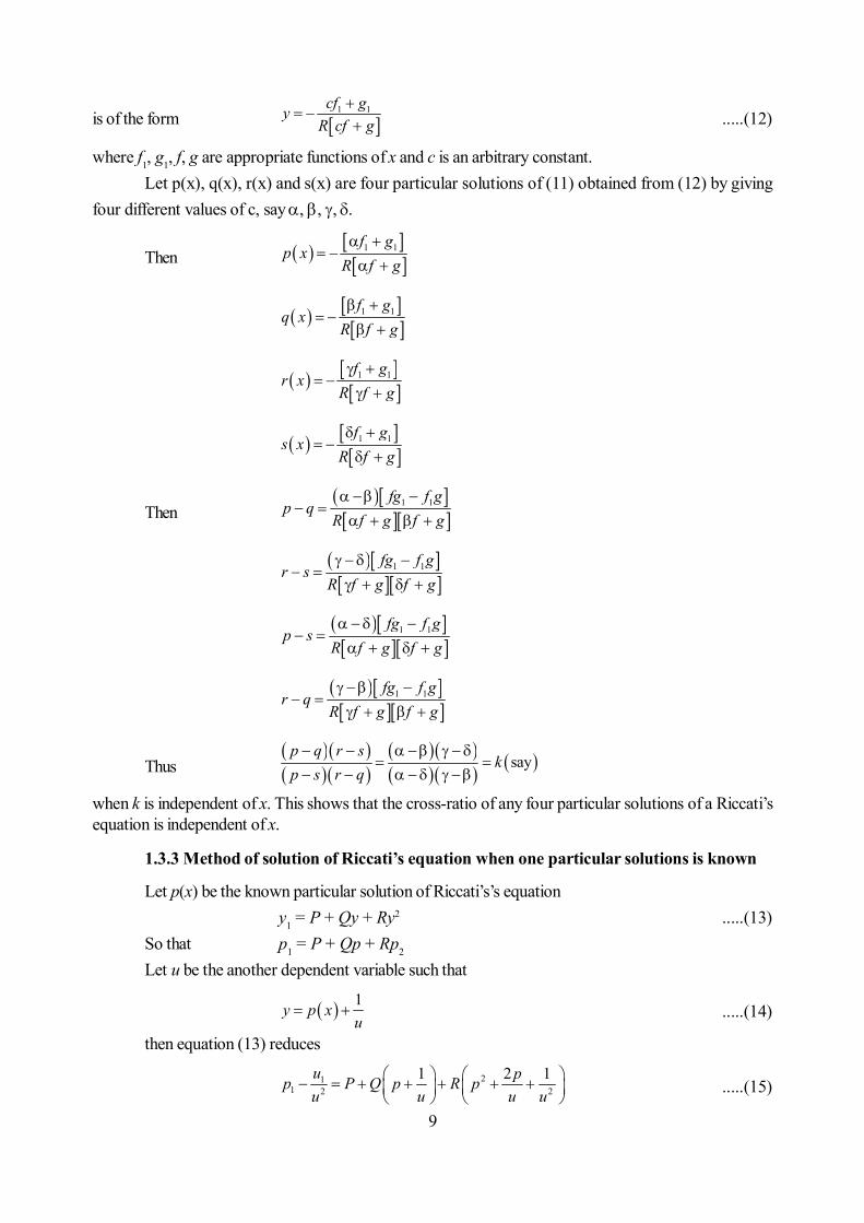
where c = A/B is an arbitrary constant. Hence the general solution of (5) is (10).1.3.2 Theorem : The cross ratio of any four particular integrals of a Riccati’s equation
is independent of x
Proof : We know that the general solution of Riccati’s equationy1 = P + Qy + Ry2 .....(11)
9
is of the form 1 1cf gy
R cf g
.....(12)
where f1, g1, f, g are appropriate functions of x and c is an arbitrary constant.Let p(x), q(x), r(x) and s(x) are four particular solutions of (11) obtained from (12) by giving
four different values of c, say , , , .
Then
1 1f gp x
R f g
1 1f gq x
R f g
1 1f gr x
R f g
1 1f gs x
R f g
Then
1 1fg f gp q
R f g f g
1 1fg f gr s
R f g f g
1 1fg f gp s
R f g f g
1 1fg f gr q
R f g f g
Thus
say
p q r s
kp s r q
when k is independent of x. This shows that the cross-ratio of any four particular solutions of a Riccati’sequation is independent of x.
1.3.3 Method of solution of Riccati’s equation when one particular solutions is known
Let p(x) be the known particular solution of Riccati’s’s equationy1 = P + Qy + Ry2 .....(13)
So that p1 = P + Qp + Rp2
Let u be the another dependent variable such that
1y p xu
.....(14)
then equation (13) reduces
211 2 2
1 2 1u pp P Q p R pu u u u
.....(15)

10
Using (14) and (15) in (13), we get
12 2
2 1u Q pRu u u u
or u1 + (Q + 2pR) u = – R
which is a linear differential equation of first order and first degree in u and x. Its integrating factor isgiven by
I.F. = e (Q + 2Rq) dx
and hence the required general solution isue (Q + 2Rq) dx = Re (Q + 2Rq) dxdx + c
where c is an arbitrary constant.
1.3.4 Method of solution of Riccati’s equation when two particular solutions are known
Let p(x) and q(x) be the two know particular solutions of Riccati’s equationy1 = P + Qy + Ry2 .....(16)
so that p1 = P + Qp + Rp2 .....(17)q1 = P + Qq + Rq2 .....(18)
From (16) and (17), we gety1 – p1 = (y – p) Q + (y2 – p2)R
or y1 – p1 = (y – p) [Q + (y + p)R]
or 1 1y p Q y p Ry p
.....(19)
Similarly from (16) and (18), we get
1 1y q Q y q Ry q
.....(20)
From (19) and (20), we get
1 1 1 1y p y q p q Ry p y q
On integration, we getlog (y – p) – log (y – q) = c + (p – q) Rdx
which is the required general solution.
1.3.5 Method of solution of Riccati’s equation when three particular solutions are known
Let p(x). q(x) and r(x) be the three known particular solutions of Riccali’s equationy1 = P + Qy + Ry2
and the corresponding values of c be , and . Then by Theorem 1.3.2, we can write
1 1f gp
R f g
1 1f gq
R f g
1 1f gr
R f g

11
then, we have constant
p q r yk
r q p y
where k is independent of x. This is the required solution of Riccati’s equation when three particularsolutions are known.
Ex.1. solve y1 = cos x – y sin x + y2
Sol. Taking y = sin x so that y1 = cos x. Substituting these in the given equation, we getcos x = cos x – sin2 x + sin2 x
This shows that y = sin x is a particular solution of given equation.
Now taking 12
1sin so that cos uy x y xu u
Using these in given equation, we get2
12
1 1cos cos sin sin sinux x x x xu u u
or 12 2
sin 1u xu u u
or sin 1du u xdx
.....(21)
Equation (21) is a linear equation of first order whose integrating factor isI.F. = esin x dx = e–cos x and hence the solution of (21) isu. e–cos x = c – e–cos x dx .....(22)
Now putting the value of
1sin
uy x
in equation (22), we getcos
cos
sin
xxe c e dx
y x
which is the required solution of given equation.Ex.2.Find the general solution of the Riccati’s equation
22 2dy
= y + ydx
whose one particular solution is (1 + tan x).Sol. The given equation is
22 2dy y ydx
.....(23)
Since (1 + tan x) is a given particular solution then taking
21 2
1 11 tan so that sec duy x y xu u dx
.....(24)
Putting (24) in (23), we get
2 2
1 1 2tandu xu dx u u

12
or 2tan 1du x udx
It is a linear differential equation of first order having integrating factorI.F. = e(2tan x)dx = e2log sec x = sec2 x
Hence the solution isu sec2 x = c – sec2 x dx = c – tan x .....(25)
From (24) and (25), the required general solution is2sec1 tan
tanxy x
c x
Ex.3. Show that there are two values of the constant for which kx
is an integral of
x2 (y1 + y2) = 2, and hence obtain the general solution.Sol. Rewriting the given equation in the standard Riccati’s form as
y1 = P + Qy + Ry2 .....(26)
21 2
2y yx
.....(27)
Let p(x) and q(x) are two particular integrals of (26), than by §1.3.4, we have
logy p
c p q Rdxy q
.....(28)
Now let 1 2so thatk ky yx x
Substituting these in (27), we get2
22 2 2
2 or 2 0 so that. 2, 1k k k k kx x x
Hence 2 1andx x
are two particular solutions of (27)
Now taking
2 1andp x q xx x
.....(29)
On comparing (26) and (27), we get R = – 1 .....(30)Using (29) and (30) in (28), we get
2 2 1log log 1 , taking log1
xy k dx c kxy x x
or2log log 3log1
xy k xxy
or 321
xy x kxy
or x3(xy –2) = k (xy + 1), where k is an arbitrary constant.
13
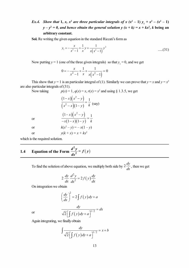
Ex.4. Show that 1, x, x2 are three particular integrals of x (x2 – 1) y1 + x2 – (x2 – 1)y – y2 = 0, and hence obtain the general solution y (x + k) = x + kx2, k being anarbitrary constant.
Sol. Re writing the given equation in the standard Riccati’s form as
2
1 2 2
1 11 1
xy y yx x x x
.....(31)
Now putting y = 1 (one of the three given integrals) so that y1 = 0, and we get
2 21 10 0
1 1x
xx x x
This show that y = 1 is an particular integral of (1). Similarly we can prove that y = x and y = x2
are also particular integrals of (31).Now taking p(x) = 1, q(x) = x, r(x) = x2 and using § 1.3.5, we get
2
2
1 11
x x y
kx x y
(say)
or
21 11 1
x x y
x x y kor k(x2 – y) = – x(1 – y)or y(k + x) = x + kx2
which is the required solution.
1.4 Equation of the Form 2
2 =d y f ydx
To find the solution of above equation, we multiply both side by 2dydx , then we get
2
22 2dy d y dyf ydx dxdx
On integration we obtain
2
2dy f y dy adx
or 1 2
2/
dy dxf y dy a
Again integrating, we finally obtain
1 2
2/
dy x bf y dy a

14
Ex.1. Solve2
32
d ysin y = cos ydx
Sol. We can write the given equation as2
22 cosec cotd y y y
dx
Now multiplying both sides by 2dydx and integrating, we get
2 2 22
2sin coscot
sindy a y ya ydx y
or 2
sin
(1 )
y dy dxa a cos y
Again integrating, we get the required solution as
11 1sin cos1
a y x caa
Ex.2. Solve2
32
d yy = cdx
Sol. We can write the given equation as2
2 3d y cdx y
Now multiplying both side by 2dydx and integrating, we get
2
2dy c adx y
or 2
y dy dxay c
Again integrating, we get the required solution asay2 = c + (ax + b)2
where a and b are two constants.
1.5 Equation not Containing y Directly
In this case general equation is given in the form
1
1 0
n n
n nd y d y dyf , ,....., , x
dxdx dx .....(1)
15
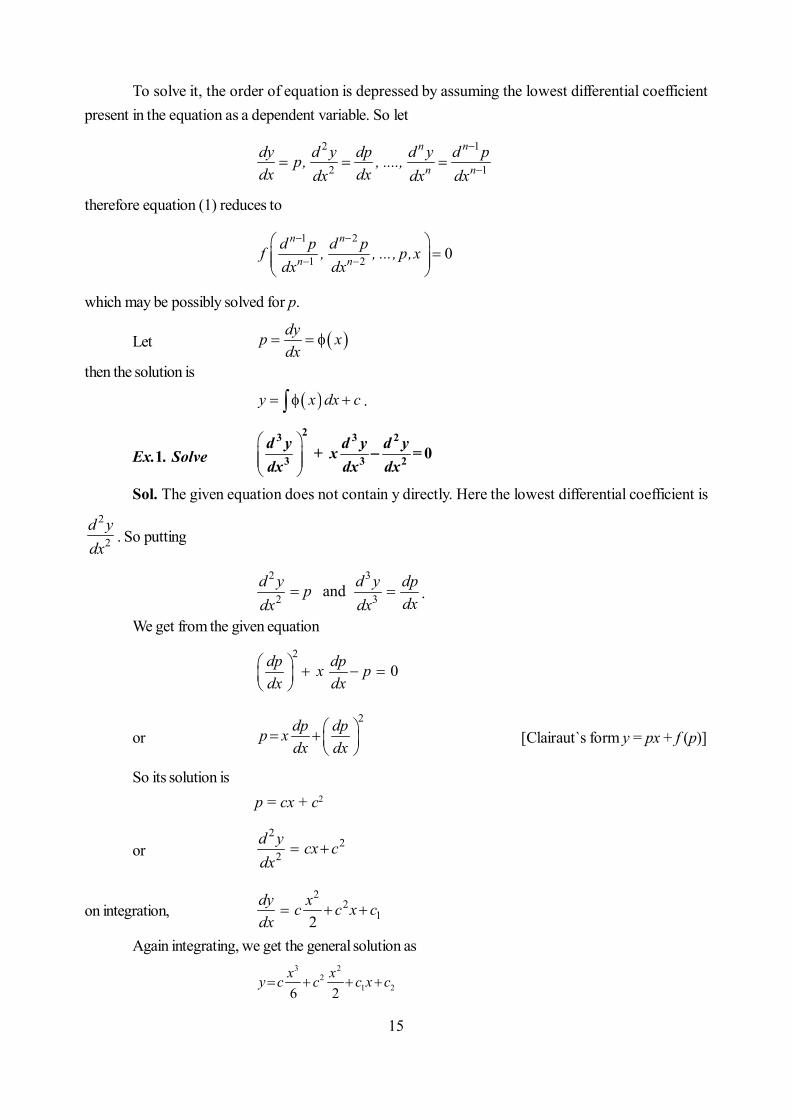
To solve it, the order of equation is depressed by assuming the lowest differential coefficientpresent in the equation as a dependent variable. So let
2 1
2 1
n n
n ndy d y dp d y d pp, , ....,dx dxdx dx dx
therefore equation (1) reduces to
1 2
1 2 0n n
n nd p d pf , , ..., p,xdx dx
which may be possibly solved for p.
Let dyp xdx
then the solution is
y x dx c .
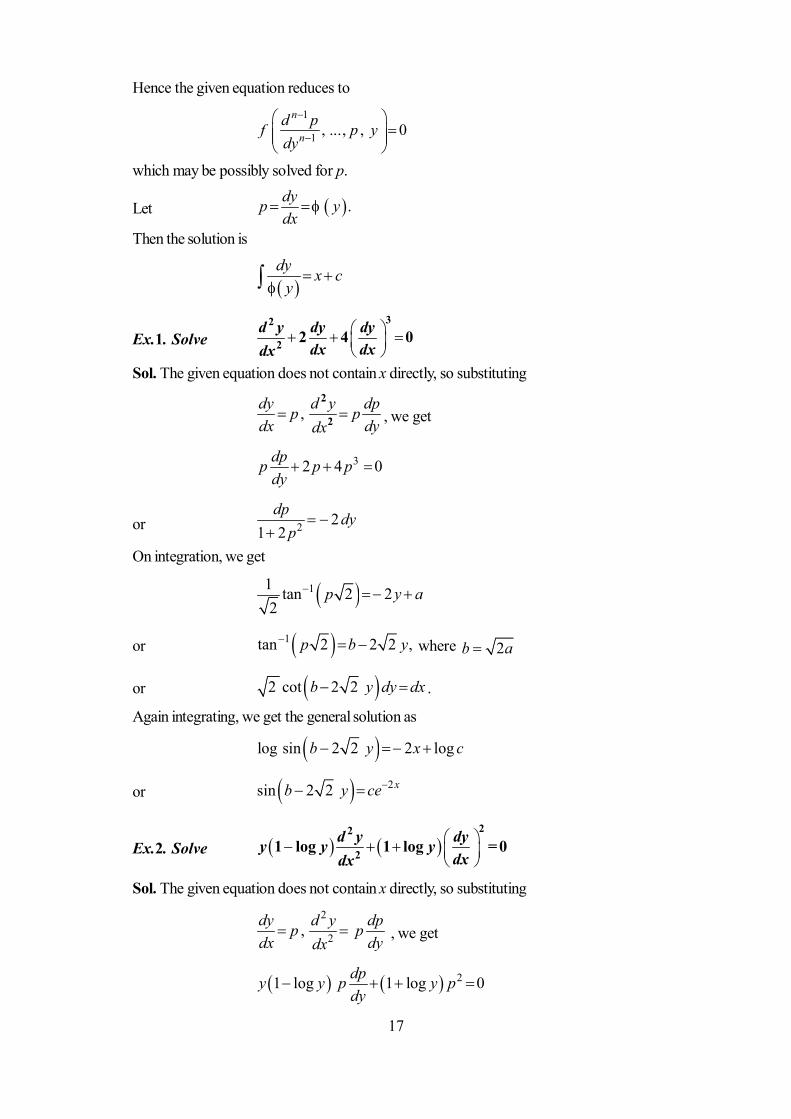
Ex.1. Solve
23 3 2
3 3 2 = 0d y d y d y+ xdx dx dx
Sol. The given equation does not contain y directly. Here the lowest differential coefficient is2
2d ydx
. So putting
2 3
2 3andd y d y dppdxdx dx
.
We get from the given equation2
0dp dpx pdx dx
or2dp dpp x
dx dx
[Clairaut`s form y = px + f (p)]
So its solution isp = cx + c2
or2
22
d y cx cdx
on integration,2
212
dy xc c x cdx
Again integrating, we get the general solution as3 2
21 26 2
x xy c c c x c
16
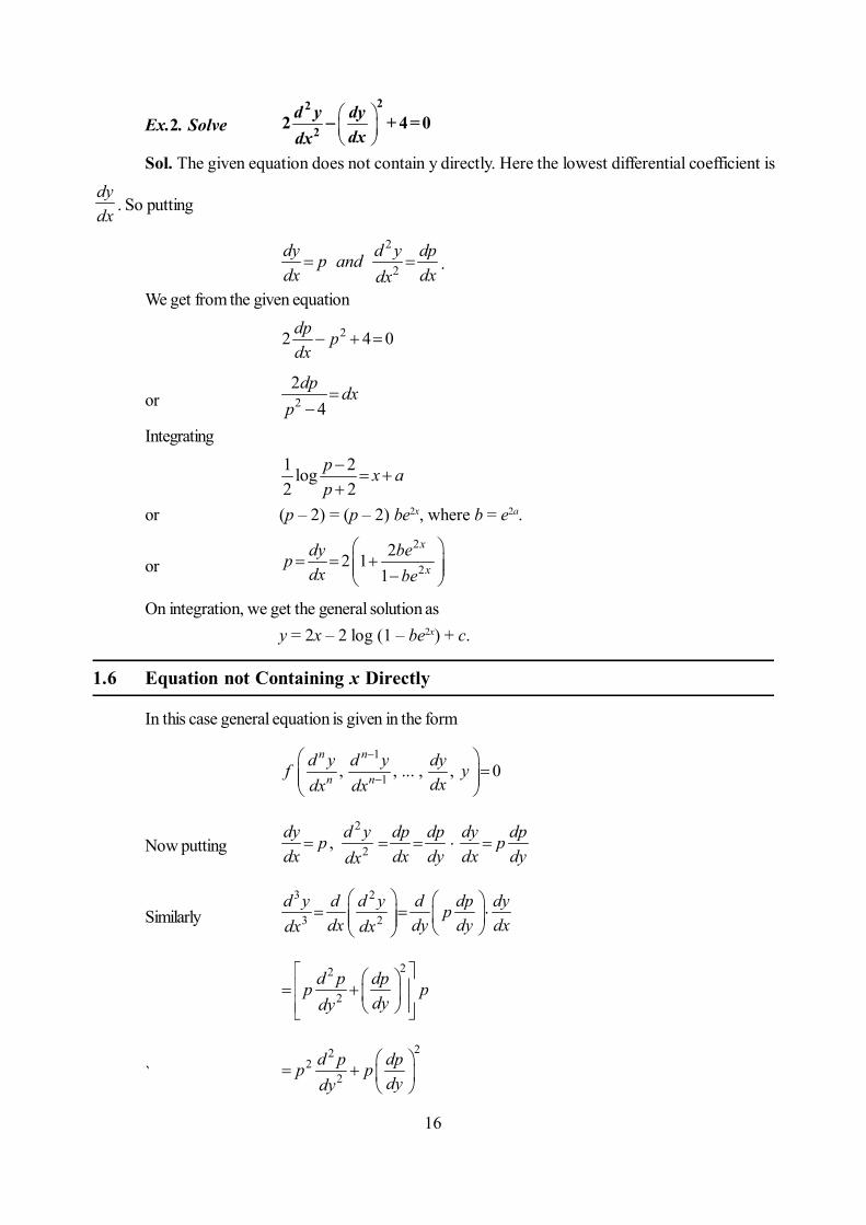
Ex.2. Solve
22
22 4 0d y dy + =dxdx
Sol. The given equation does not contain y directly. Here the lowest differential coefficient isdydx . So putting
2
2dy d y dpp anddx dxdx
.
We get from the given equation
22 4 0dp pdx
or 22
4dp dx
p
Integrating
1 2log2 2
p x ap
or (p – 2) = (p – 2) be2x, where b = e2a.
or2
222 1
1
x
xdy bepdx be
On integration, we get the general solution asy = 2x – 2 log (1 – be2x) + c.
1.6 Equation not Containing x Directly
In this case general equation is given in the form
1
1, , ... , , 0n n
n nd y d y dyf y
dxdx dx
Now putting2
2,dy d y dp dp dy dpp pdx dx dy dx dydx
Similarly3 2
3 2d y d d y d dp dyp
dx dy dy dxdx dx
22
2d p dpp p
dydy
`22
22
d p dpp pdydy
17
Hence the given equation reduces to1
1 , ..., , 0n
nd pf p ydy
which may be possibly solved for p.
Let .dyp ydx
Then the solution is
dy x c
y
Ex.1. Solve
32
2 2 4 0d y dy dydx dxdx
Sol. The given equation does not contain x directly, so substituting
,dy d y dpp pdx dydx
2
2 , we get
32 4 0dpp p pdy
or 2 21 2
dp dyp
On integration, we get
11 tan 2 22
p y a
or 1tan 2 2 2 ,p b y where 2b a
or 2 cot 2 2b y dy dx .
Again integrating, we get the general solution as
log sin 2 2 2 logb y x c
or 2sin 2 2 xb y ce
Ex.2. Solve
22
21 log 1 log = 0d y dyy y ydxdx
Sol. The given equation does not contain x directly, so substituting2
2,dy d y dpp pdx dydx
, we get
21 log 1 log 0dpy y p y pdy
18
or 1 log
0.1 log
ydp dyp y y
On integration, we get by substituting log y = t
log log 2 log log 1 constantp y y
or 2log 1dyp ay ydx
or 2log 1dy a dx
y y
Again integrating , we get the general solution as
1
log 1ax b
y
or 11 log yax b
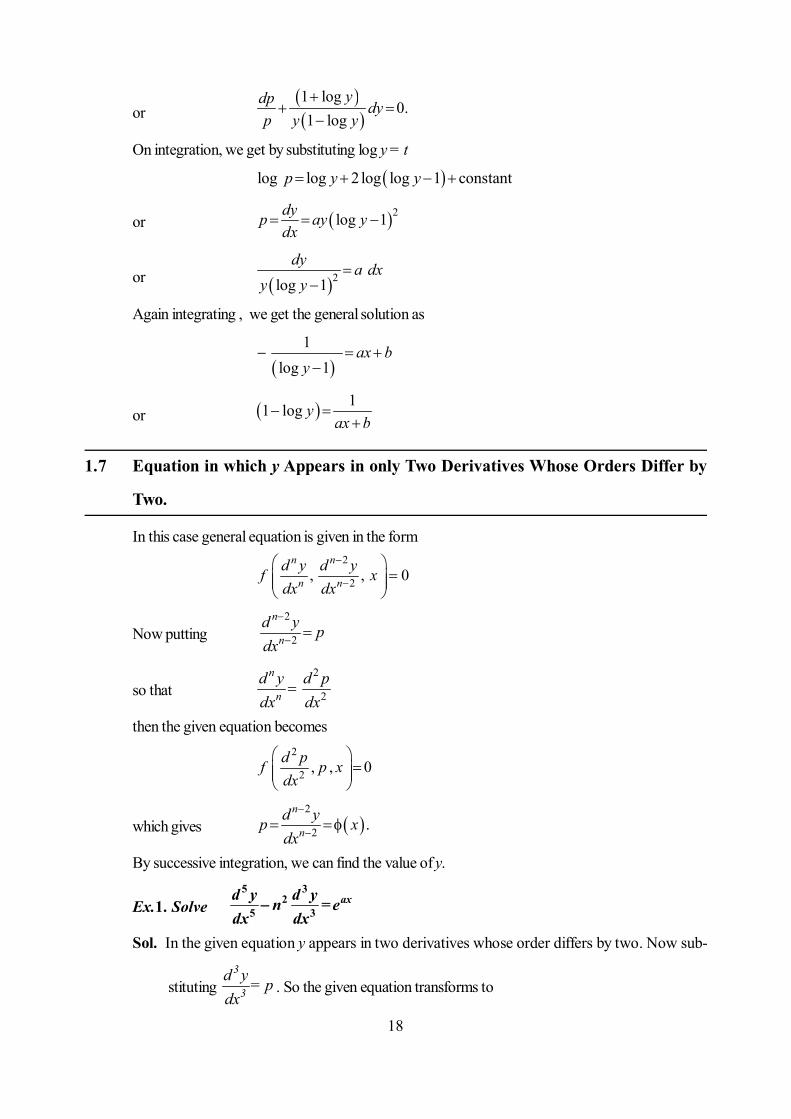
1.7 Equation in which y Appears in only Two Derivatives Whose Orders Differ by
Two.
In this case general equation is given in the form2
2, , 0n n
n nd y d yf xdx dx
Now putting2
2
n
nd y pdx
so that2
2
n
nd y d pdx dx
then the given equation becomes2
2 , , 0d pf p xdx
which gives 2
2 .n
nd yp xdx
By successive integration, we can find the value of y.
Ex.1. Solve5 3
25 3
axd y d yn = edx dx
Sol. In the given equation y appears in two derivatives whose order differs by two. Now sub-
stituting 3
3d y = pdx
. So the given equation transforms to

19
22
ax2
d p n p = edx
whose solution will be
3
1 23 2 2
axnx nxd y ep c e c e
dx a n
On integration, we get
2
1 232 2 2
axnx nxc cd y ee e c
n ndx a a n
Again integrating
1 2
3 42 2 2 2 2
axnx nxc cdy ee e c x c
dx n n a a n
which on integration gives the general solution as
2
1 23 4 53 3 3 2 2 2
axnx nxc c e xy e e c c x c
n n a a x
1.8 Equation in which y Appears in only Two Derivatives Whose Orders Differ byUnity
In this case general equation is given in the form
1
1, , 0n n
n nd y d yf xdx dx
Now putting1
1
n
nd y pdx
so thatn
nd y dp .
dxdx
Hence the given equation reduces to
0dpf , p , xdx
This is an equation of first order. We can here easily find the value of p in terms of x as
1
1
n
nd yp x .dx
By successive integration, we get the general solution.
20
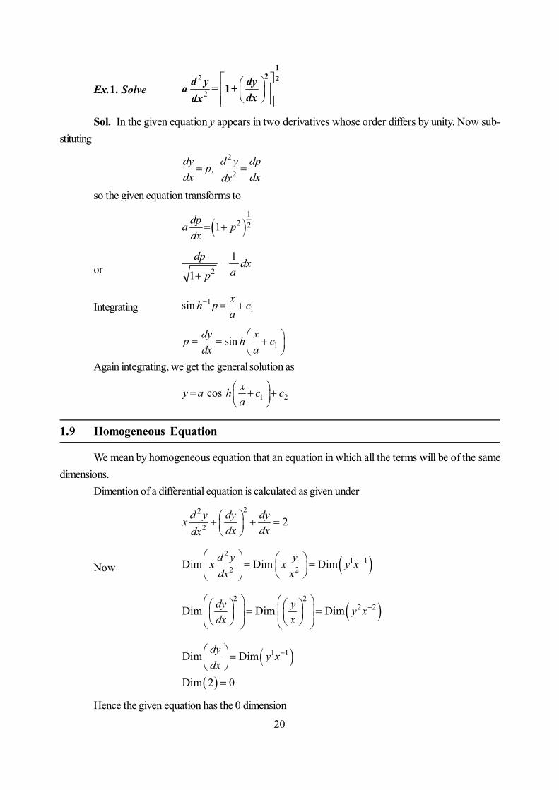
Ex.1. Solve2
2
12 2
1d y dya = +dxdx
Sol. In the given equation y appears in two derivatives whose order differs by unity. Now sub-stituting
2
2dy d y dpp,dx dxdx
so the given equation transforms to
1
2 21dpa pdx
or 2
1
1
dp dxap
Integrating 11sin xh p c
a
1sindy xp h cdx a
Again integrating, we get the general solution as
1 2cos xy a h c ca
1.9 Homogeneous Equation
We mean by homogeneous equation that an equation in which all the terms will be of the samedimensions.
Dimention of a differential equation is calculated as given under22
2 2d y dy dyxdx dxdx
Now 2
1 12 2Dim Dim Dimd y yx x y x
dx x
2 2
2 2Dim Dim Dimdy y y xdx x
1 1Dim Dim
Dim 2 0
dy y xdx
Hence the given equation has the 0 dimension
21
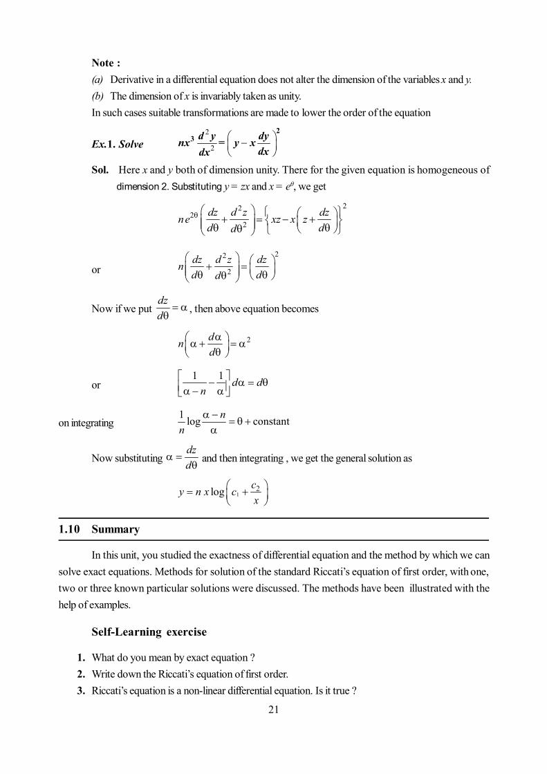
Note :(a) Derivative in a differential equation does not alter the dimension of the variables x and y.(b) The dimension of x is invariably taken as unity.In such cases suitable transformations are made to lower the order of the equation
Ex.1. Solve2
2
23 d y dynx = y x
dxdxSol. Here x and y both of dimension unity. There for the given equation is homogeneous of
dimension 2. Substituting y = zx and x = e, we get
222
2dz d z dzne xz x zd dd
or22
2dz d z dznd dd
Now if we put dzd
, then above equation becomes
2dnd
or1 1 d d
n
on integrating1 log constantnn
Now substituting dzd
and then integrating , we get the general solution as
12log cy n x cx
1.10 Summary
In this unit, you studied the exactness of differential equation and the method by which we cansolve exact equations. Methods for solution of the standard Riccati’s equation of first order, with one,two or three known particular solutions were discussed. The methods have been illustrated with thehelp of examples.
Self-Learning exercise
1. What do you mean by exact equation ?2. Write down the Riccati’s equation of first order.3. Riccati’s equation is a non-linear differential equation. Is it true ?

22
1.11 Answers of Self-Learning Exercise
1. A differential equation which is integrable directly.
2. 2dy P Qy Rydx
, where P, Q, R are functions of x or constants.
3. True
1.12 Exercise
1. Solve the following differential equations :
(a)22
2 22 3 0d y dyx y x y y
dxdx
[Ans. 2 5 12
25cxy c x ]
(b) 2
22 2 1 0d y dy dyy xdx dxdx
[Ans. 21 2y xy c x c ]
(c)22
2cos sin cos 1d y dy dyy y y xdx dxdx
[Ans. 2
1 21
sin2
xxy x c c e
]
2. Solve the following differential equations :
(a) 3 2 2 211 2 ,x x y x y xy x is an integral [Ans.
4 3
22
3x x xcy x
]
(b) 21 ,dy ydx
tan x is an integral [Ans. tan tan 1y c x c x ]
(c) 3 2 2 21x y x y y x [Ans. y (ce2/x – 1) = x + cxe2/x]
(d) 211 2 1 2 0x x y x y yh x , x is a solution [Ans.
2x cy
x c
]
3. Solve :
(a)2
21d y
dx ay [Ans. 1 21 4
1 1 23 2 2x a y c y c c ]
(b)2 2
2 2 0d y adx y
[Ans. 21 1 1 1 2
1
1 log 1 2c y y c y c y ac x cc
]
4. Solve :
(a)22
2 1d y dydxdx
[Ans. 1 2cosy h x c c ]

23
(b) 22
221 1 0d y dyx
dxdx
[Ans. 211 logy cx c x c c ]
(c)32
2 0d y dy dydx dxdx
[Ans. 11 2sin xy c e c ]
(d)23 2 2
23 2 22 d y d y d yx a
dx dx dx
[Ans. 5 2
12 32
1
415
c x ay c x c
c
]
5. Solve :
(a)22
22
d y dyy ydxdx
[Ans. 21 2sin 2y c h x c ]
(b)22
2 0d y dyadxdx
[Ans. 1 2aye c x c ]
(c)22
2 1 0d y dyydxdx
[Ans. 2 21 2 0y x c x c ]
(d)22
22 logd y dyy y y
dxdx
[Ans. 1 2log x xy c e c e ]
(e)
1 222 22 22
2 2dy d y dy d yy n adx dxdx dx
[Ans. 1 22 2
21 cxcy n a c c e ]
6. Solve :
(a)4 2
24 2 0d y d ya
dx dx [Ans. 1 2 3 4
ax axy c e c e c x c ]
(b)4 2
2 24 2 0d y d yx a
dx dx [Ans.
5 2 2 241 2 3 1 4 1 4cy c c x x c x a a
x
when a < 12 and
5 2 21 2 3
4
1cos 4 1 log2
xy c c x c x ac
when a >
12 ]
7. Solve :
(a)2
2 0d y dyxdxdx
[Ans. 1 2logy c x c ]
(b)3 2
3 2 2d y d ydx dx
[Ans. 5 21 2 315 8y x c c x c ]
24
8. Solve :
(a)22
2 3d y dy dyxy x ydx dxdx
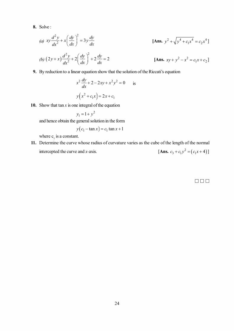
[Ans. 2 4 4 41 2y y c x c x ]
(b) 22
22 2 2 2d y dy dyy xdx dxdx
[Ans. 2 21 2xy y x c x c ]
9. By reduction to a linear equation show that the solution of the Riccati’s equation
2 2 22 2 0dyx xy x ydx
is
21 12y x c x x c
10. Show that tan x is one integral of the equation2
1 1y y and hence obtain the general solution in the form
1 1tan tan 1y c x c x
where c1 is a constant.11. Determine the curve whose radius of curvature varies as the cube of the length of the normal
intercepted the curve and x-axis. [Ans. 23 1 1 4 c c y c x ]

25
Unit 2 : Total Differential EquationsStructure of the Unit
2.0 Objective
2.1 Introduction
2.2. Necessary and Sufficient Condition for Integrability of the Total Differential Equation
2.2.1 Theorem
2.3 Methods of Solving Total Differential Equations
2.3.1 Method of Inspection
2.3.2 Method for Homogeneous Equations
2.3.3 Working Rule for Solving Homogenous Equations
2.3.4 Method of Auxiliary Equations
2.3.5 General Method
2.4 Geometrical meaning of Pdx + Qdy + Rdz = 0
2.5 Equations Containing More Than Three Variables
2.6 Method for Obtaining Solution Involving Four Variables
2.7 Total Differential Equation of Second Order
2.8 Summary
2.9 Answers of Self Learning Exercise
2.10 Exercise
2.0 Objective
In this unit, you will learn various methods for solving different types of total differential equa-tions. Some of the methods are : Method of inspection, method for homogeneous equations, method ofAuxiliary equations and general method. You will also study the geometrical meaning and method forsolving total differential equations involving three or four variables.
2.1 Introduction
In this unit, we propose to discuss differential equations with one independent variable and more
than one dependent variables.
26
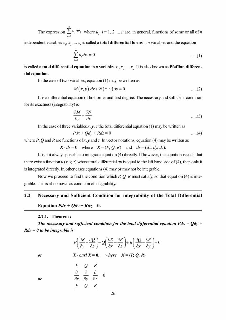
The expression 1
,n
i ii
u dx where ui , i = 1, 2 .... n are, in general, functions of some or all of n
independent variables x1, x2 .... xn is called a total differential forms in n variables and the equation
10
n
i ii
u dx
.....(1)
is called a total differential equation in n variables x1, x2 .... xn. It is also known as Pfaffian differen-tial equation.
In the case of two variables, equation (1) may be written as
, , 0M x y dx N x y dy .....(2)
It is a differential equation of first order and first degree. The necessary and sufficient conditionfor its exactness (integrability) is
M Ny x
.....(3)
In the case of three variables x, y, z the total differential equation (1) may be written asPdx + Qdy + Rdz = 0 .....(4)
where P, Q and R are functions of x, y and z. In vector notations, equation (4) may be written asX dr = 0 where X = (P, Q, R) and dr = (dx, dy, dz).
It is not always possible to integrate equation (4) directly. If however, the equation is such thatthere exist a function u (x, y, z) whose total differential du is equal to the left hand side of (4), then only itis integrated directly. In other cases equations (4) may or may not be integrable.
Now we proceed to find the condition which P, Q, R must satisfy, so that equation (4) is inte-grable. This is also known as condition of integrability.
2.2 Necessary and Sufficient Condition for integrability of the Total Differential
Equation Pdx + Qdy + Rdz = 0.
2.2.1. Theorem :The necessary and sufficient condition for the total differential equation Pdx + Qdy +
Rdz = 0 to be integrable is
0R Q R P Q PP Q Ry z x z x y
or X curl X = 0, where X = (P, Q, R)
or0
P Q R
x y zP Q R

27
Proof : Condition is necessary :Let u (x, y, z) = C .....(1)be an integral of total differential equation
Pdx + Qdy + Rdz = 0 .....(2)Then total differential du of (1), must be equal to Pdx + Qdy + Rdz, or it multiplied by a factor.
But we know the differentiation of (1) is
u u udu dx dy dzx y z
.....(3)
Since (1) is an integral of (2), therefore P, Q, R must be proportional to ux
, uy and
uz
.
So, , , sayu x u y u z x y zP Q R
, ,u u uP Q Rx y z
.....(4)
From the first two parts of (4), we get
2 2u u uP Q
y y x x y x y x
orP QP Qy y x x
orP Q Q Py x x y
.....(5)
Similarly, we can write
Q R R Qz y y z
.....(6)
andR P P Rx z z x
.....(7)
Multiplying (5), (6) and (7) by R, P and Q respectively and adding, we get
0R Q R P Q PP Q Ry z x z x y
.....(8)
This is the condition for the integrability of total differential equation (2).
Sufficient Condition :
Now we prove that if the condition (8) is satisfied, then the equation (2) will have a solution ofthe form (1).
Now if the condition (8) is satisfied for P, Q, R of the equation (2) then it can be easily verifiedthat the same condition will hold for the coefficients of
28
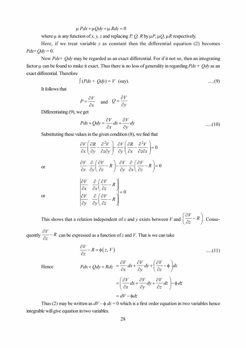
0Pdx Qdy Rdz
where is any function of x, y, z and replacing P, Q, R by P, Q, R respectively.Here, if we treat variable z as constant then the differential equation (2) becomes
Pdx+Qdy = 0.Now Pdx+ Qdy may be regarded as an exact differential. For if it not so, then an integrating
factor can be found to make it exact. Thus there is no loss of generality in regarding Pdx + Qdy as anexact differential. Therefore
(Pdx + Qdy) = V (say). .....(9)It follows that
VPx
and VQy
Differentiating (9), we getV VPdx Qdy dx dyx y
.....(10)
Substituting these values in the given condition (8), we find that2 2
0V R V V R Vx y z y y x z x
or 0V V V VR Rx y z y x z
or0
V V Rx x zV V Ry y z
This shows that a relation independent of x and y exists between V and V Rz
. Conse-
quently V Rz
can be expressed as a function of z and V. That is we can take
,V R z Vz
.....(11)
Hence Pdx Qdy Rdz V V Vdx dy dzx y z
V V Vdx dy dz dzx y z
dV dz
Thus (2) may be written as dV – dz = 0 which is a first order equation in two variables henceintegrable will give equation in two variables.
29
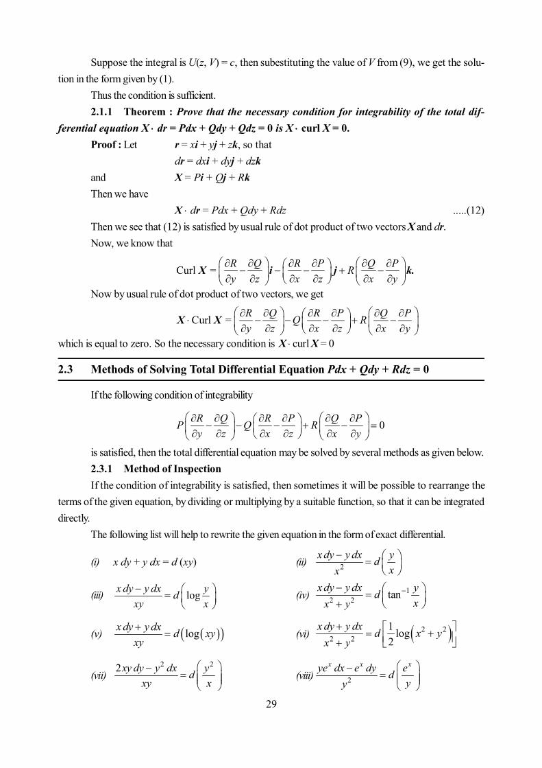
Suppose the integral is U(z, V) = c, then subestituting the value of V from (9), we get the solu-tion in the form given by (1).
Thus the condition is sufficient.2.1.1 Theorem : Prove that the necessary condition for integrability of the total dif-
ferential equation X dr = Pdx + Qdy + Qdz = 0 is X curl X = 0.Proof : Let r = xi + yj + zk, so that
dr = dxi + dyj + dzkand X = Pi + Qj + RkThen we have
X dr = Pdx + Qdy + Rdz .....(12)Then we see that (12) is satisfied by usual rule of dot product of two vectors X and dr.Now, we know that
Curl = R Q R P Q PRy z x z x y
X i j k.
Now by usual rule of dot product of two vectors, we get
Curl = R Q R P Q P Q Ry z x z x y
X X
which is equal to zero. So the necessary condition is X curl X = 0
2.3 Methods of Solving Total Differential Equation Pdx + Qdy + Rdz = 0
If the following condition of integrability
0R Q R P Q PP Q Ry z x z x y
is satisfied, then the total differential equation may be solved by several methods as given below.2.3.1 Method of InspectionIf the condition of integrability is satisfied, then sometimes it will be possible to rearrange the
terms of the given equation, by dividing or multiplying by a suitable function, so that it can be integrateddirectly.
The following list will help to rewrite the given equation in the form of exact differential.
(i) x dy + y dx = d (xy) (ii) 2x dy y dx yd
xx
(iii) logx dy y dx ydxy x
(iv) 1
2 2 tanx dy y dx ydxx y
(v) logx dy y dx d xyxy
(vi) 2 22 2
1 log2
x dy y dx d x yx y
(vii)2 22xy dy y dx yd
xy x
(viii) 2
x x xye dx e dy edyy
30
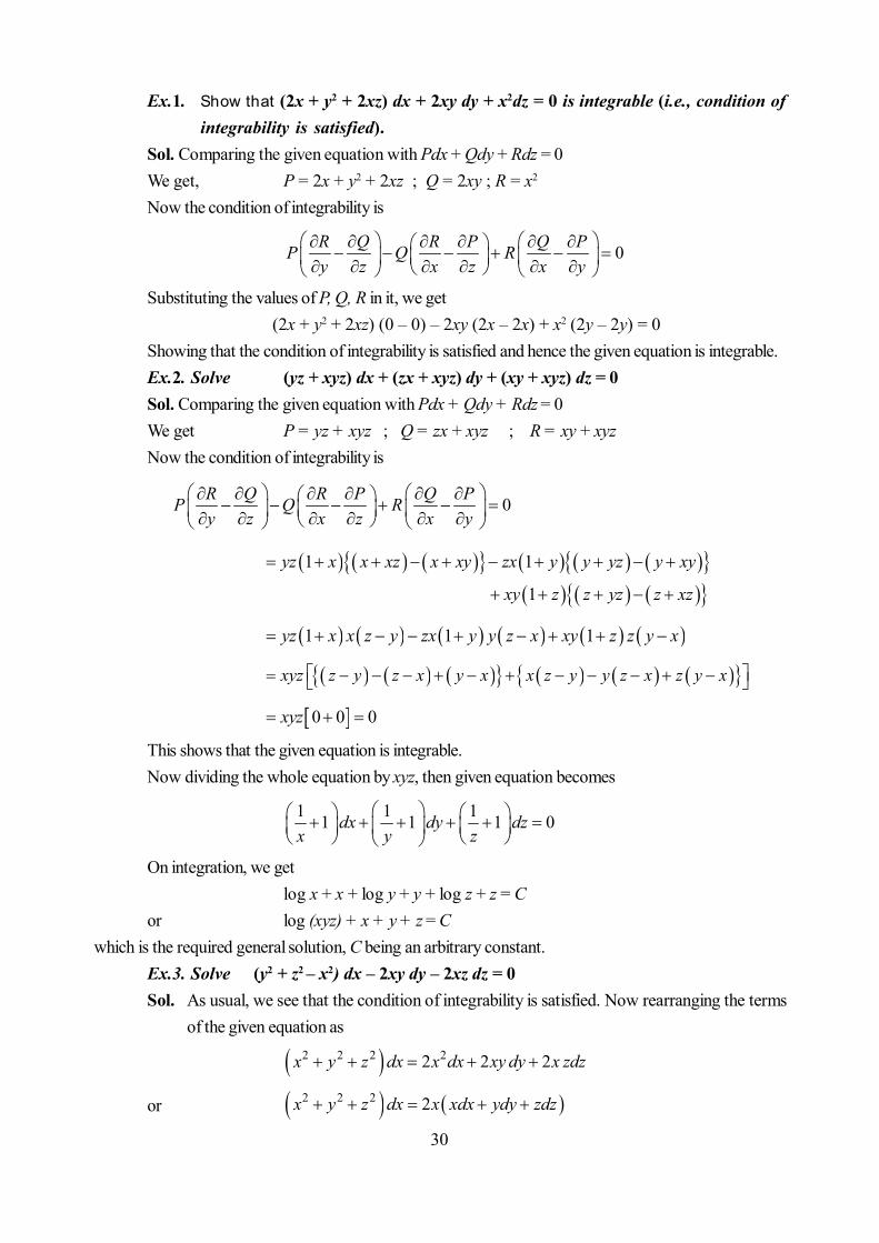
Ex.1. Show that (2x + y2 + 2xz) dx + 2xy dy + x2dz = 0 is integrable (i.e., condition ofintegrability is satisfied).
Sol. Comparing the given equation with Pdx + Qdy + Rdz = 0We get, P = 2x + y2 + 2xz ; Q = 2xy ; R = x2
Now the condition of integrability is
0R Q R P Q PP Q Ry z x z x y
Substituting the values of P, Q, R in it, we get(2x + y2 + 2xz) (0 – 0) – 2xy (2x – 2x) + x2 (2y – 2y) = 0
Showing that the condition of integrability is satisfied and hence the given equation is integrable.Ex.2. Solve (yz + xyz) dx + (zx + xyz) dy + (xy + xyz) dz = 0Sol. Comparing the given equation with Pdx + Qdy + Rdz = 0We get P = yz + xyz ; Q = zx + xyz ; R = xy + xyzNow the condition of integrability is
0R Q R P Q PP Q Ry z x z x y
1 1
1
yz x x xz x xy zx y y yz y xy
xy z z yz z xz
1 1 1yz x x z y zx y y z x xy z z y x
xyz z y z x y x x z y y z x z y x
0 0 0xyz
This shows that the given equation is integrable.Now dividing the whole equation by xyz, then given equation becomes
1 1 11 1 1 0dx dy dzx y z
On integration, we getlog x + x + log y + y + log z + z = C
or log (xyz) + x + y + z = Cwhich is the required general solution, C being an arbitrary constant.
Ex.3. Solve (y2 + z2 – x2) dx – 2xy dy – 2xz dz = 0Sol. As usual, we see that the condition of integrability is satisfied. Now rearranging the terms
of the given equation as
2 2 2 22 2 2x y z dx x dx xy dy x zdz
or 2 2 2 2x y z dx x xdx ydy zdz
31
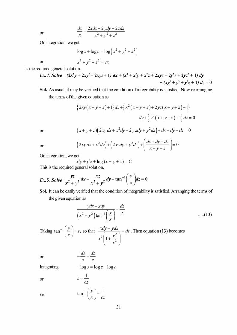
or 2 2 22 2 2dx xdx ydy zdz
x x y z
On integration, we get
2 2 2log log logx c x y z
or 2 2 2x y z cx is the required general solution.
Ex.4. Solve (2x2y + 2xy2 + 2xyz + 1) dx + (x3 + x2y + x2z + 2xyz + 2y2z + 2yz2 + 1) dy + (xy2 + y3 + y2z + 1) dz = 0
Sol. As usual, it may be verified that the condition of integrability is satisfied. Now rearrangingthe terms of the given equation as
2
2
2 1 2 1
1 0
xy x y z dx x x y z yz x y z
dy y x y z dz
or 2 22 2 0x y z xy dx x dy y zdy y dz dx dy dz
or 2 22 2 0dx dy dzxy dx x dy yzdy y dzx y z
On integration, we getx2y + y2z + log (x + y + z) = C
This is the required general solution.
Ex.5. Solveyz xz ydx dy dz
xx y x y1
2 2 2 2 tan 0
Sol. It can be easily verified that the condition of integrability is satisfied. Arranging the terms ofthe given equation as
2 2 1tan
ydx xdy dzy zx yx
.....(13)
Taking 1tan ,y sx
so that 2
221
xdy ydx dsyxx
. Then equation (13) becomes
ords dzs z
Integrating log log logs z c
or1scz
i.e. 1 1tan yx cz

32
which gives1tany
x cz
This is the required general solution.2.3.2 Method for Homogeneous EquationsThe equation Pdx + Qdy + Rdz = 0 is called a homogeneous equation if P, Q, R are homoge-
neous functions of x, y, z of the same degree. In such a case one variable is separated from the othertwo by the substitution
x = uz, y = vz .....(14)then dx = udz + zdu, dy = vdz + zdv .....(15)Further, let
1 2, , ,n nP z f u v Q z f u v and 3 ,nR z f u v .....(16)Hence the given equation Pdx + Qdy + Rdz = 0 becomes
11 2 1 2 3, , , , , 0n nz f u v du f u v dv z uf u v vf u v f u v dz
On multiplying by z, we get
2 11 2 1 2 3, , , , , 0n nz f u v du f u v dv z uf u v vf u v f u v dz .....(17)
Now following two cases arise :Case I : Px + Qy + Rz = 0If Px + Qy + Rz = 0 that is by substituting the values of x, y from (14) and P, Q, R from (16) in
it, we find
11 2 3, , , 0nz uf u v vf u v f u v
then the coefficient of dz in equation (17) will become zero and hence it reduces to
1 2, , 0f u v du f u v dv .....(18)
which can be integrated easily.Case II : Px + Qy + Rz 0In this case the coefficient of dz will not be zero and therefore equation (17) may be written as.
1 2
1 2 3
, ,0
, , ,f u v du f u v dv dz
zuf u v vf u v f u v
...(19)
Now since the given equation Pdx + Qdy + Rdz = 0 is integrable so equation (19) will be anexact differential and hence this equation may be integrated easily.
2.3.3 Working Rule for Solving Homogeneous Equations(i) First of all verify the condition of integrability.(ii) If Px + Qy + Rz = 0, then substitute x = uz, y = vz and solve
(iii) If Px + Qy + Rz 0 then 1
Px Qy Rz will be an integrating factor of the homogeneous
equation Pdx + Qdy + Rdz = 0. After multiplying this equation by this integrating factor and rearrangingthe terms we can integrate the equation by inspection.

33
Ex.6. Solve z dx z yz dy y yz xz dz2 2 22 2 0
Sol. Comparing the given equation with the standard equation Pdx + Qdy + Rdz = 0, we getP = z2, Q = z2 – 2yz, R = 2y2 – yz – xz
The given equation is homogeneous of degree 2. Now first of all we test the condition of inte-grability
R Q R P Q PP Q Ry z x z x y
2 2 24 2 2 2 2 2 0 0z y z z y z yz z z y yz xz
2 3 3 26 3 3 6 0yz z z yz
Hence the condition of integrability is satisfied
Further, 2 2 2 2 2 22 2 0Px Qy Rz xz yz y z y z yz xz
Therefore, we substitutex = uz, y = vz
Hence dx = udz + zdu, dy = vdz + zdvand the given equation reduces to
2 2 2 21 2 2 0z udz zdu z v vdz zdv z v v u dz
or du + (1 – 2v) dv = 0Integrating, we get
u + v – v2 = Cor xz + yz – y2 = cz2
This is the required general solution.
Ex.7. Solve yz z dx xzdy xydz2 0
Sol. On comparing the given equation with Pdx + Qdy + Rdz = 0,we have P = yz + z2, Q = – xz, R = xyHere the given equation is homogeneous of degree 2 and the condition of integrability is satisfied
(do your self)Now Let D = Px + Qy + Rz
= x (yz + z2) – xyz + xyz = xz (y + z) 0
Multiplying the given equation by integrating factor 1/D, we get
2
0yz z dx xz dy xy dz
D
.....(17)
Now d D d xz y z z dx xdz y z xz dy dz
or 2d D z y z dx x y z dz xz dy
34
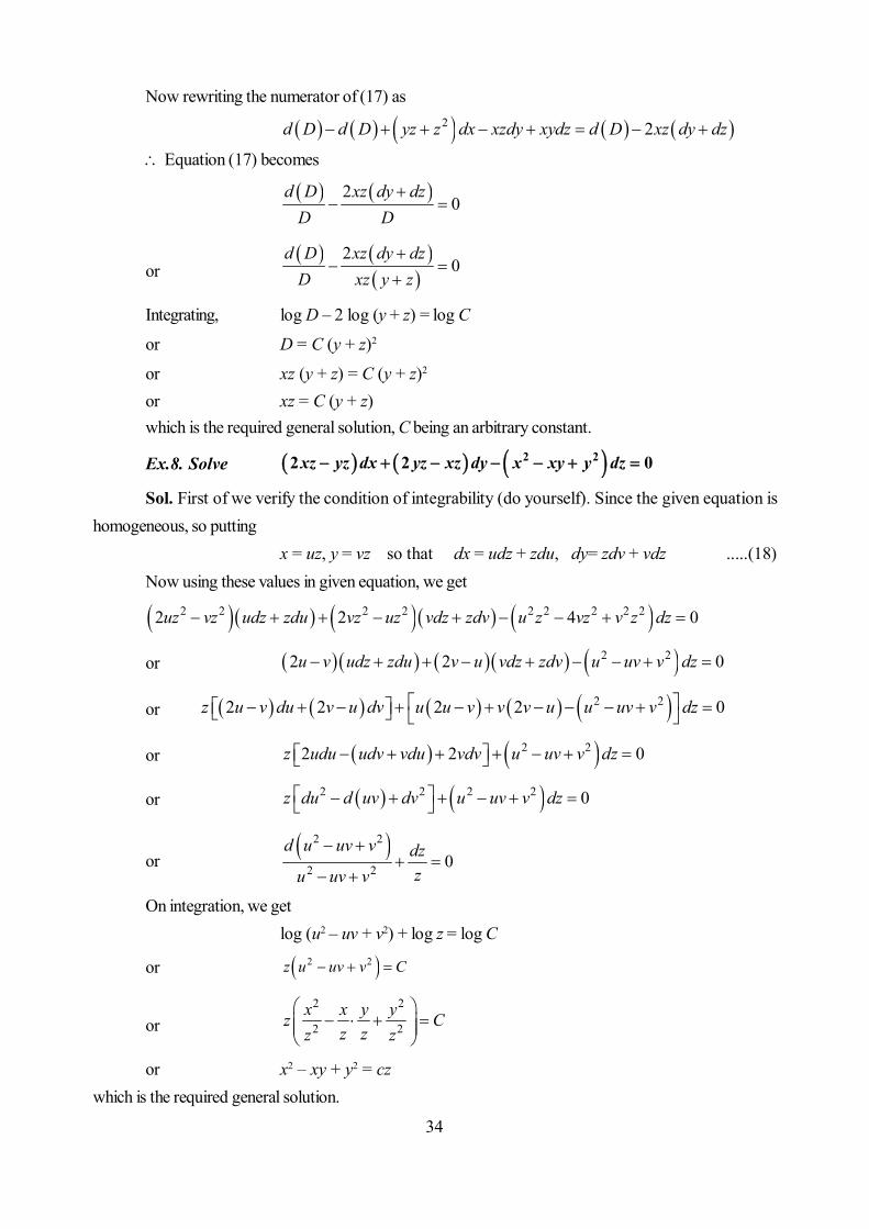
Now rewriting the numerator of (17) as
2 2d D d D yz z dx xzdy xydz d D xz dy dz
Equation (17) becomes
20
d D xz dy dzD D
or
2
0d D xz dy dz
D xz y z
Integrating, log D – 2 log (y + z) = log C
or D = C (y + z)2
or xz (y + z) = C (y + z)2
or xz = C (y + z)which is the required general solution, C being an arbitrary constant.
Ex.8. Solve xz yz dx yz xz dy x xy y dz2 22 2 0
Sol. First of we verify the condition of integrability (do yourself). Since the given equation ishomogeneous, so putting
x = uz, y = vz so that dx = udz + zdu, dy= zdv + vdz .....(18)Now using these values in given equation, we get
2 2 2 2 2 2 2 2 22 2 4 0uz vz udz zdu vz uz vdz zdv u z vz v z dz
or 2 22 2 0u v udz zdu v u vdz zdv u uv v dz
or 2 22 2 2 2 0z u v du v u dv u u v v v u u uv v dz
or 2 22 2 0z udu udv vdu vdv u uv v dz
or 2 2 2 2 0z du d uv dv u uv v dz
or 2 2
2 2 0d u uv v dz
zu uv v
On integration, we getlog (u2 – uv + v2) + log z = log C
or 2 2z u uv v C
or2 2
2 2x x y yz C
z zz z
or x2 – xy + y2 = czwhich is the required general solution.

35
Ex.9. Solve yz y z dx zx x z dy xy x y dz 0
Sol. First of all verify the condition of integrability (do your self). Since the given equation ishomogeneous, we put
x = uz, y = vz so that dx = zdu + udz, dy = zdv + vdz .....(19)Substituting these in the given equation, we get
v (v + 1) z3 (zdu + udz) + u (u + 1) z3 (zdv + vdz) + uv (u + v) z3dz = 0or [v (v + 1) du + u (u + 1) dv] z4 + [uv(v + 1) + uv (u + 1) + uv (u + v)] z3dz = 0or [v (v + 1) du + u (u + 1) dv] z4 + 2uv (u + v + 1) z3dz = 0Dividing above equation by uv (u + v + 1) z4, we get
1 12 0
1 1v du u dv dz
u u v v u v z
or1 1 1 1 2 0
1 1dzdu dv
u u v v u v z
or 2 01
du dv du dv dzu v u v z
On integration, we get
log log log 1 2log logu v u v z C
or uvz2 = C (u + v + 1)
or 2 1x y x yz Cz z z z
by using (9)
or xyz = C (x + y + z)this is the required general solution.
2.3.4 Method of Auxiliary EquationsLet Pdx + Qdy + Rdz = 0 .....(20)
by the given equation. Its condition of integrability is
0R Q R P Q PP Q Ry z x z x y
. .....(21)
On comparing (20) and (21), we obtain simultaneous equations, known as auxiliary equations.
dx dy dzR Q R P Q Py z x z x y
.....(22)
For solving (22) let u = c1 and v = c2 be their two integrals. After finding the value of Adu + Bdv= 0 and comparing it with the given equation, the values of A and B will be obtained. Integration of Adn+ Bdv = 0, will give the required solution.
This method will fail if ,R Q R Py z x z
and Q Px y
36
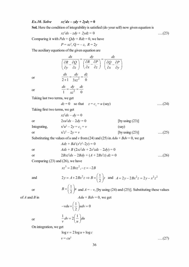
Ex.10. Solve xz3dx – zdy + 2ydz = 0Sol. Here the condition of integrability is satisfied (do your self) now given equation is
xz3dx – zdy + 2ydz = 0 .....(23)Comparing it with Pdx + Qdy + Rdz = 0, we have
P = xz3, Q = – z, R = 2yThe auxiliary equations of the given equation are
dx dy dzR PR Q Q Px zy z x y
or 22 1 03dx dy dz
xz
or 21 0dx dy dz
xz
Taking last two terms, we getdz = 0 so that z = c1 = u (say) ......(24)
Taking first two terms, we getxz2dx – dy = 0
or 2xu2dx – 2dy = 0 [by using (23)]Integrating, x2u2 – 2y = c2 = v (say)or x2z2 – 2y = v [by using (23)] .....(25)Substituting the values of u and v from (24) and (25) in Adu + Bdv = 0, we get
Adz + Bd (x2z2–2y) = 0or Adz + B (2xz2dx + 2x2zdz – 2dy) = 0or 2Bxz2dx – 2Bdy + (A + 2Bx2z) dz = 0 .....(26)Comparing (23) and (26), we have
3 22 , 2xz Bxz z B
and 2 12 22
y A Bx z B z
and 2 2 22 2 2A y Bx z y x z
or12
B u
and A = – v, [by using (24) and (25)]. Substituting these values
of A and B in Adu + Bdv = 0, we get
1 02
vdu udv
or1 12dv duv u
On integration, we getlog 2log logv u c
v = cu2 .....(27)
37
Putting the values of u and v from (24) and (25) in (27), we get2 2 22x z y cz
which is the required general solution.2.3.5 General MethodStep I : Let the condition of integrability is satisfied for the given equation
0Pdx Qdy Rdz .....(28)Step II : Treating one of the variables of (28), say z, as a constant then dz = 0 and the given
equation is reduced toPdx + Qdy = 0
Integrating it, keeping z as constant. If necessary the help of an integrating factor may be taken.Let the result so obtained be
u (x, y, z) = f (z) .....(29)where f (z) is a function of z alone. This is possible because the arbitrary function f (z) is con-
stant with respect to x and y.Step III : Now we differentiate (29) totally with respect to x, y, z and then compare the result
with the given equation (28). We will get a relation between df and dz. If the of df and dz involve func-tions of x and y, it would be possible to eliminate them with the help of (22). Thus we shall get an equa-tion in df and dz which will be independent of x and y.
Step IV : The values of f (z) will be obtained by integrating the above equation. After sustitutingit in (32), we get the complete solution.
Remark : General method, for solving the total differential equation of the typePdx + Qdy + Rdz = 0
should be adopted only when the equations are non-homogeneous and the method of inspectionfails.
Ex.11. Solve 3x2dx + 3y2dy – (x3 + y3 + e2z) dz = 0Sol. Here, the condition of integrability is satisfied. Let us treat z as constant, so that dz = 0.
Then the given equation become3x2dx + 3y2dy = 0
On integration, we getx3 + y3 = f (z) (say) .....(30)
where the constant of integration has been taken as a function f (z) as we have treated z asconstant.
Now differentiating (30), we have
2 23 3 0x dx y dy f z dz .....(31)Comparing (31) with the given equation, we get
3 3 2zf z x y e
or 2zf z f z e [by using (30)]
38
or 2zdf f edz
, which is a linear equation having integrating factor as
1 dz zIF e e . Hence the solution is
2z z z zf z e e e dz c e c or 2z zf z e ce
or 3 3 2z zx y e ce [by using (30)]Which is the required general, C being an arbitrary constant.
Ex.12. x z y x y x ye y e dx e z e dy e e y e z dz 0
Sol. Here, the condition of integrability is satisfied. Let us treat z as constant so that dz = 0.Then the given equation becomes
0x z y ze y dx e dy e zdy e dx
On integration. we get
x y ze y e z e x f z .....(32)
Now differentiating equation (32), we obtain
x z y x y ze y e dx e z e dy e e x dz f z dz .....(33)
Comparing (33) with the given equation, we get
y z y x ye e x f z e e y e z
which gives
x y zf z e y e z e x f z (by 32)
ordf fdz
Integrating, we getf (z) = cez
Putting the value of f (z) from equation (32), we get the required general solution asexy + eyz + ezx = cez
Ex.13. Solve 2 2cos sin cos siny z x x x dx x z y y y dy
sin sin cos 0xy y x x y xy z dz
Sol. Here, the condition of integrability, is satisfied. Let us treat z as constant so that dz = 0.Then the given equation becomes
2 2cos sin cos sin 0y z x x x dx x z y y y dy
or 2 2cos sin cos sin 0x x x y y ydx dy
x y

39
orsin sin 0x yd d
x y
On integration, we get
sin sinx y f zx y
.....(34)
where the constant of integration has been taken as a function f (z) as we have treated z asconstant.
Now differentiating (34), we get
2 2cos sin cos sinx x x y y ydx dy f z dz
x y
or 2 2 2 2cos sin cos sin 0zy x x x dx zx y y y dy x y z f z dz .....(35)Comparing (35) with the given equation, we have
2 2 sin sin cosx y z f z xy y x x y xy z
or sin sin cos cosx yz f z z f z zx y
[by using (34)]
or1 cosdf zf
dz z z , which is a linear equation having integrating factor (IF)
as
1 logz dz zIF e e z and the solution is
cos sinzz f z z dz c z cz
orsin sin sinx yz c z
x y
[by using (34)]
which is the required general solution, c being an arbitrary constant.
Self Learning Exercise-I
1. Write down pfaffian differential equation in n variables.2. Write the condition when an equation of the type Mdx + Ndy = 0 become exact.3. What is the condition of integrability for the equation Pdx + Qdy + Rdz = 0 ?4. Which equations are called homogeneous ?
2.4 Geometrical Meaning of Pdx + Qdy + Rdz = 0
We know that direction cosines of the tangent at a point (x, y, z) on a curve are proportional todx, dy, dz. Therefore, the differential equation Pdx + Qdy + Rdz = 0 .....(1)signifies that the tangent to a curve at the point (x, y, z) is perpendicular to a line, whose direction co-sines are proportional to P, Q, R.

40
Whereas the simultaneous equations
dx dy dzP Q R .....(2)
express that the tangent to a curve at a point (x, y, z) is parallel to a line with direction cosines propor-tional to P, Q, R.
We thus have two sets of curve, and if they intersect, they intersect at right angle. Now we dis-cuss two cases.
Case I : If the equation Pdx + Qdy + Rdz = 0 is integrable, it means that family of surfaces canbe obtained such that all curves on it are perpendicular to the curves represented by the equation (2) atall points where curves cut the surface. Since the solution of equation (1) will be of the form (x, y, z) =C and that of (2) will be of the form f1 (x, y, z) = C1 and f2 (x, y, z) = C2 , it means that in this case aninfinite number of surfaces can be drawn to cut orthogonally a doubly infinite set of curves.
Case II : If equation (1) is not integrable than the curves represented by dx dy dzP Q R may
not admit of such a family of orthogonal surfaces.Ex.1. Solve Find the system of curves satisfying the differential equating.
x yxdx ydy c dza b
2 2
2 21 0 ....(3)
which lie on the surface
x y za b c
2 2 2
2 2 21 ....(4)
Sol. Equation of the given surface can be written as2 2 2
2 2 2 1x y za b c
....(5)
with the help of (3), the given equation can be written asxdx+ydy +zdz=0
on Integration, we getx2 + y2 + z2 = k ....(6)
Hence the required system of curves will be given by the intersection of (5) and (6).
Ex.2. Find the differential equation of the family of twisted cubic curves y = ax2,y2 = bzx. Show that all these curves cut orthogonally the family of ellipsoidsx2 + 2y2 + 3z2 = c2.
Sol. Family of twisted cubic curves as given in question isy = ax2 .....(7)y2 = bzx ....(8)
On differentiating (7), we getdy = 2ax dx

41
or dy 2 y dxx
[by using (7)]
or 2ydx - xdy = 0 ....(9)Now similarly, differentiating (8), we obtain
2ydy = b(zdx + xdz)
or2
2 yydy ( zdx xdz )zx
[by using (8)]
or yz dx - 2zx dy + xy dz = 0 ....(10)From (9) and (10), we get
2 2 2 22dx dy dz
( zx ) y ( x )yzx y xy
or 2 2 32dx dy dz
xyzx y xy
or 2 3dx dy dzx y z
which are the required differential equations of the family of curves.The differential equations of the surfaces which are cut orthogonally by the given curves is
x dx + 2y dy + 3z dz = 0Integrating, we get
x2 + 2y2 + 3z2 = k = c2 (say)
2.5 Equations Containing More than Three Variables
Let us consider an equation of the formPdx + Qdy + Rdz + Tdt = 0 ....(1)
Treating t as constant, so that dt = 0, then equation (1) becomesPdx + Qdy + Rdz = 0 ....(2)
Condition of integrability for equation (2) will be
0R Q R P Q PP Q Ry z x z x y
....(3)
Similarly If we take z, x and y as constant, then we get dz = 0, dx = 0, dy = 0. The condition ofintegrability in these cases will be
0T Q T P Q PP Q Ty t x t x y
....(4)
0T R T Q R QQ R Tz t y t y z
....(5)
and 0T P T R P RR P Tx t z t z x
....(6)
42
Hence we see that in the case of more than three variables, the condition of integrability must besatisfied for the coefficients of all the terms taken three at a time.
Here we note that only three of the relations (3), (4), (5) and (6) are independent and the fourthone can be derived from the remaining three.
2.6 Method for Obtaing Solution Involving Four Variables
If the condition of integrability is satisfied, then the solution the total differential equation can beobtained by two methods.
Method 1. By Inspection : In this method we can arrange the coefficients in such way that thegiven equation is directly integrable.
Method 2. In this method, we take any two of the four variables constant. The equation is inte-grated and the constant of integration is taken as the function of those variables which were kept con-stant. The result is compared with the given equation after obtaining its differential and in such a way the
values of constants of integration are obtained. This will give the complete solution.
Ex.1. Solve (2x + y2 + 2xz) dx + 2xy dy + x2dz = dt.
Sol. We can write the given equation as(2x + y2 + 2xz) dx + 2xy dy + x2dz – dt = 0
we can easily verify the condition of integrability as given by equations (3), (4), (5) and (6) of§2.5.
Now the given equation can be written as 2xdx + (y2dx + 2xy dy) + (2xzdx + x2dz) - dt = 0.Which on integration gives the complete solution as x2 + xy2 + x2z - t = c.
Ex.2. Solve z (y + z) dx + z (t - x) dy + y (x - t) dz + y (y + z) dt = 0
Sol. On comparing the given question by the standard equation Pdx + Qdy + Rdz + Tdt = 0,we get
P = z(y + z), Q = z(t – x), R = y(x – t), T = y(y + z)
Here we can easily show that the conditions of integrability (equations (3), (4), (5) and (6) of§2.5) are satisfied.
Now we solve the given question by treating two variables as constant. Treating y and z as con-stants so that dy = 0 and dz = 0. Then the given equation reduces to
z(y + z) dx + y(y + z) dt = 0
or zdx + ydt = 0
On integration, we get
zx + yt = f (x, z) ( say) .....(7)
Now on differentiation (7), we get
zdx + tdy + xdz + ydt = df
or (y + z) (zdx + tdy + xdz + ydt) = (y + z) df
43
or z(y + z) dx + t(y + z) dy + x(y + z) dz + y(y + z) dt = (y + z) df .....(8)
Comparing (8) with the given equation, we have
t(y + z) dy + x(y + z) dz – (y + z) df = z(t – x) dy + y(x – t) dz
or (ty + xz) dy + (ty + xz) dz = (y + z) df
or (ty + xz) (dy + dz) = (y + z) df
or f (dy + dz) = (y + z) df [by using (7)]
ordt dy dzf y z
.....(9)
Integration of (9) yieldslog f = log (y + z) + log c
or f = c(y + z)or zx + yt = c(y + z) [by using (7)]
2.7 Total Differential Equation of Second Degree
It the given equation be of the formAdx2 + Bdy2 + Cdz2 + 2Ddydz + 2Edzdx + 2Fdxdy = 0
where A, B, C, D, E and F are functions of x, y, and z then it can be easily resolved into factors, ifABC + 2DEF – AD2 – BE2 – CF2 = 0
Let the two factors bePdx + Qdy + Rdz = 0
and Pdx + Qdy + Rdz = 0The solutions of either of these may be obtained by the methods discussed earlier. The two gen-
eral solutions taken together constitute the complete solution.
Ex.1. Solve (xdx + ydy + zdz)2z = {(z2x2y2) (xdx + ydy + zdz) dz}
Sol. We can factorize the given equation as
(xdx + ydy + zdz) {z(xdx + ydy + zdz) – (z2 – x2 – y2) dz} = 0
i.e., xdx + ydy + zdz = 0 .....(1)and z(xdx + ydy + zdz) – z2dz + (x2 + y2) dz = 0 .....(2)On integration of (1), we get
x2 + y2 + z2 = c1 .....(3)
To obtain the integral of (2), the equation may be written as
z(xdx + ydy) + (x2 + y2) dz = 0
or z2(2xdx + 2ydy) + (x2 + y2) 2zdz = 0
On integration, we get
z2(x2 + y2) = c2 .....(4)

44
Hence the required solution is
(x2 + y2 + z2 – c1) (z2x2 + z2y2 – c2) = 0
Self Learning Exercise-II
1. The direction cosines of the tangent at a point (x, y, z) on a curve are proportional to _, _, _.2. What is the equation of family of twisted cubic curves ?
2.8 Summary
In this unit, you studied about the condition of integrability of total differential equation and vari-ous methods for solving it. Now you must be knowing about the geometrical meaning of Pdx + Qdy +Rdz = 0 and methods of finding solution of total differential equation containing three or more than threevariables
2.9 Answers of Self Learning Exercises
Exercise I
1.1
0n
i ii
u dx
, where ui (i = 1, 2 .......... n) are n functions of some or all of n independent vari-
ables x1, x2 ,....., xn.
2.M Ny x
3. 0R Q R P Q PP Q Ry z x z x y
4. Equation Pdx + Qdy + Rdz = 0 is called homogeneous if P, Q, R are homogenous functions ofx, y, z of the same degree.
Exercise II
1. dx, dy, dz2. y = ax2, y2 = bzx
2.10 Exercise
Solve the following differential equations
1. (2x2 + 2xy + 2xz2 + 1) dx + dy + 2zdz = 0 [Ans. 2 2xe x y z c ]
2. xdy – ydx + 2x2z dz = 0 [Ans. 2y z cx ]
3. (y + a)2 dx + zdy – (y + a)dz = 0 [Ans. z = (x + c) (y + a)]
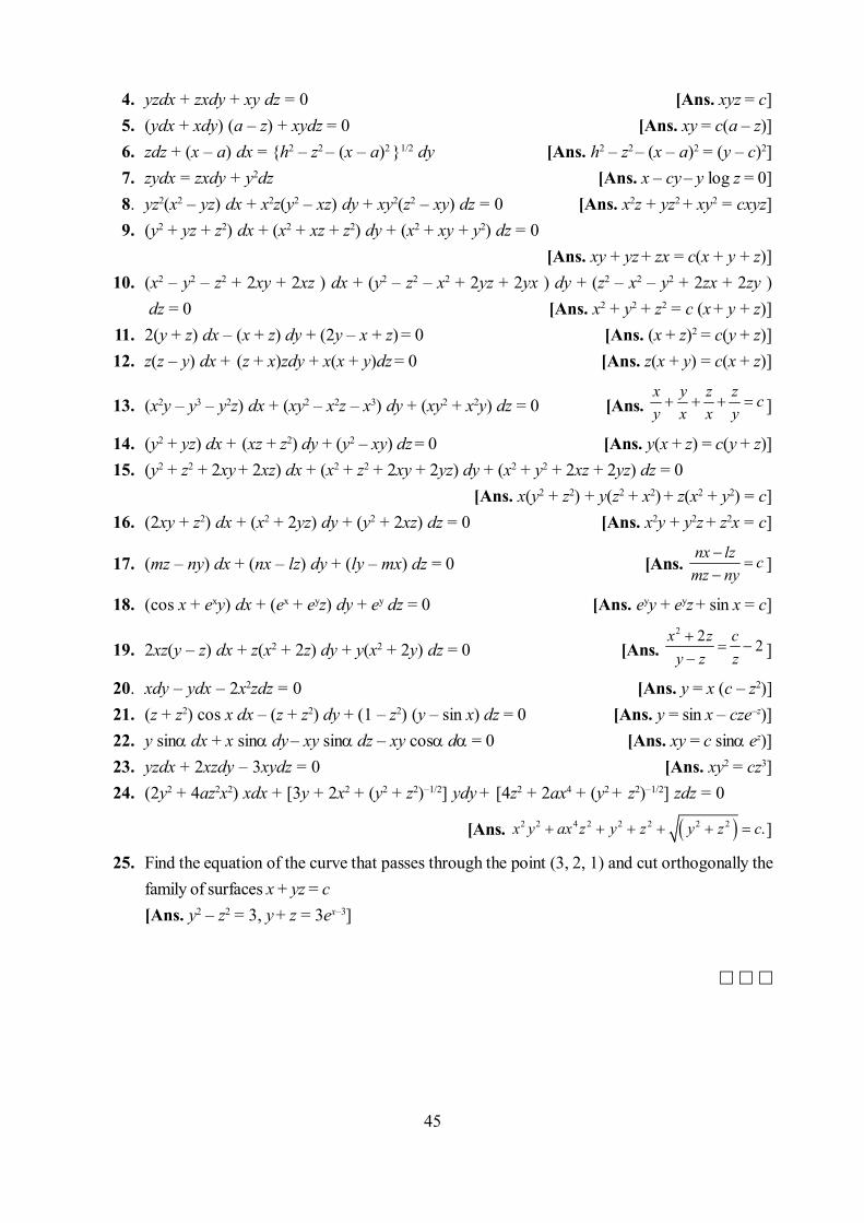
45
4. yzdx + zxdy + xy dz = 0 [Ans. xyz = c]5. (ydx + xdy) (a – z) + xydz = 0 [Ans. xy = c(a – z)]6. zdz + (x – a) dx = {h2 – z2 – (x – a)2 }1/2 dy [Ans. h2 – z2 – (x – a)2 = (y – c)2]7. zydx = zxdy + y2dz [Ans. x – cy – y log z = 0]8. yz2(x2 – yz) dx + x2z(y2 – xz) dy + xy2(z2 – xy) dz = 0 [Ans. x2z + yz2 + xy2 = cxyz]9. (y2 + yz + z2) dx + (x2 + xz + z2) dy + (x2 + xy + y2) dz = 0
[Ans. xy + yz + zx = c(x + y + z)]10. (x2 – y2 – z2 + 2xy + 2xz ) dx + (y2 – z2 – x2 + 2yz + 2yx ) dy + (z2 – x2 – y2 + 2zx + 2zy )
dz = 0 [Ans. x2 + y2 + z2 = c (x + y + z)]11. 2(y + z) dx – (x + z) dy + (2y – x + z) = 0 [Ans. (x + z)2 = c(y + z)]12. z(z – y) dx + (z + x)zdy + x(x + y)dz = 0 [Ans. z(x + y) = c(x + z)]
13. (x2y – y3 – y2z) dx + (xy2 – x2z – x3) dy + (xy2 + x2y) dz = 0 [Ans. x y z z cy x x y ]
14. (y2 + yz) dx + (xz + z2) dy + (y2 – xy) dz = 0 [Ans. y(x + z) = c(y + z)]15. (y2 + z2 + 2xy + 2xz) dx + (x2 + z2 + 2xy + 2yz) dy + (x2 + y2 + 2xz + 2yz) dz = 0
[Ans. x(y2 + z2) + y(z2 + x2) + z(x2 + y2) = c]16. (2xy + z2) dx + (x2 + 2yz) dy + (y2 + 2xz) dz = 0 [Ans. x2y + y2z + z2x = c]
17. (mz – ny) dx + (nx – lz) dy + (ly – mx) dz = 0 [Ans. nx lz cmz ny
]
18. (cos x + exy) dx + (ex + eyz) dy + ey dz = 0 [Ans. eyy + eyz + sin x = c]
19. 2xz(y – z) dx + z(x2 + 2z) dy + y(x2 + 2y) dz = 0 [Ans. 2 2 2x z cy z z
]
20. xdy – ydx – 2x2zdz = 0 [Ans. y = x (c – z2)]21. (z + z2) cos x dx – (z + z2) dy + (1 – z2) (y – sin x) dz = 0 [Ans. y = sin x – cze–z)]22. y sin dx + x sin dy – xy sin dz – xy cos d = 0 [Ans. xy = c sin ez)]23. yzdx + 2xzdy – 3xydz = 0 [Ans. xy2 = cz3]24. (2y2 + 4az2x2) xdx + [3y + 2x2 + (y2 + z2)–1/2] ydy + [4z2 + 2ax4 + (y2 + z2)–1/2] zdz = 0
[Ans. 2 2 4 2 2 2 2 2 .x y ax z y z y z c ]
25. Find the equation of the curve that passes through the point (3, 2, 1) and cut orthogonally thefamily of surfaces x + yz = c[Ans. y2 – z2 = 3, y + z = 3ex–3]
46
Unit 3 : Partial Differential Equations of Second order,Monge’s Method
Structure of the Unit
3.0 Objective
3.1 Introduction
3.2 Solution of P.D.E. of Second order by Inspection.
3.3 Exercise – I
3.4 Monge’s Method for Solving Equation of the Type Rr + Ss + Tt = V
3.5 Monge’s Method for Solving Equation of the Type Rr + Ss + Tt + U(rt – s2) = V
3.6 Summary
3.7 Answers of self-Learning Exercises
3.8 Exercise – II
3.0 Objective
The purpose of this unit is to discuss partial differential equations of order two with variable co-
efficients. Here you will learn how a large class of second order partial differential equations may be
solved by using the methods applicable for solving ordinary differential equations ? You will also study
Monge’s method for solution of some special type of second order partial differential equations.
3.1 Introduction
A partial differential equation (P.D.E) is said to be of order two, if it involves at least one of the
differential coefficients r, s, t and none of order higher than two. The general form of a second order
partial differential equation in two independent variables x, y is given as
as F(x, y, z, p, q, r, s, t) = 0 ;
where2 2 2
2 2, , , ,z z z z zp q r s tx y x yx y
The most general linear partial differential equation of second order in two independent variablex and y with variable coefficient is given as
Rr + Ss + Tt + Pp + Qq + Zz = Fwhere R, S, T, P, Q, Z, F are functions of x and y only and not all R, S, T are zero.

47
3.2 Solution of P.D.E. of Second Order by Inspection
Before taking up the general equation of second degree P.D.E., we discuss the solution of simpleproblems which can be integrated merely by inspection. On two successive integral of given P.D.E., weget the general solution which is a relation in x, y, z. To understand this, we discuss the following prob-lems.
Ex.1. Solve t + s + q = 0Sol. We can write the given problem as
2 2
2 0z z zx y yy
Integrating with respect to y, treating x as constant, we get
z z z f xy x
or p + q = f (x) – z
which is the form of standard Lagrange’s linear equation Pp + Qq = R, so the auxiliary equation will be
1 1dx dy dz
f x z
from first two terms, we obtainx – y = c1 (constant) .....(1)
and from first and last terms, we have
dz z f xdx
.....(2)
which is linear differential equation of first order having integrative factor ex.Hence the solution of (2) will be
z ex = f (x) exdx + c2 (constant)Therefore the required solution of given equation will be (by using (1)]
zex – (x) = (x – y)where c2 is a function of c1 or of (x – y).
Ex.2. Solve t – qx = x2
Sol. We can write the given problem as
2q qx xy
.....(3)
which is linear in q and y having integrating factor e–xdy = e–xy. Therefore the solution of (3) isq e–xy = x2 e–xy dy + f (x) (as x is constant)
or q e–xy = –xe–xy + f (x)
or
xyz x f x e
yAgain integrating with respect to y (treating x as constant), we get.
1 .xyz xy f x e xx

48
Ex.3. Solve xx ty2=
Sol. We can write the given problem as2 2
2 2z z x
x y y y
Integrating with respect to y (treating x as constant), we get
z z x f xx y y
or xp q f xy
which is the form of standard Lagrange’s linear equation Pp + Qq = R, so the auxiliary equation will be
1 1dx dy dz
x y f x
From first two terms, we obtainx + y = c1 (constant) .....(4)
and from first and last terms, we have
xdz dx f x dxy
or 1
xdz dx f x dxc x
[by using (4)]
or 1
1 cdz dx f x dxc x
On integrating, we get
1 1 2logz x c c x f x dx c or 1 logz x c y x F x y
where c2 is a function of c1 or of (x + y).Ex.4. Solve rx = (n – 1) pSol. We can write the given problem as
2
12z z
x nxx
or
2
2 1z
nxz xx
Now integrating both sides with respect to x treating y as constant, we get
1log 1 log logz n x f yx

49
or 11
nz x f yx
Again integrating w.r.t. x treating y as constant, we obtain
1 2
nxz f y f yn
Ex.5. Solve 2yq + y2t = 1Sol. We can write the given problem as
22 1qyq yy
or 2 1y qy
Now integrating both side with respect to y treating x as constant, we gety2q = f1(x)
or 121zq f x
y y
Again integrating with respect to y, we obtain
1 21 .z f x f xy
Ex.6. Show that a surface passing through the circle z = 0, x2 + y2 = 1 and satisfyingthe differential equation s = 8xy is z = (x2 + y2)2 – 1
Sol. We can write the given differential equation as2
8z z xyx y x y
Integrating with respect to x, we get
24z x y f yy
Again integrating with respect to y, we obtain
2 212z x y f y dy x
or 2 22 12 z x y y x .....(5)
where 2 y f y dy where 1 and 2 are two arbitrary functions.
Now given circle isx2 + y2 = 1, z = 0
Putting z = 0 in (5), we get2x2y2 + 2 (y) + 1 (x) = 0 .....(6)
Now, x2 +y2 = 1 (x2 + y2)2 = 12
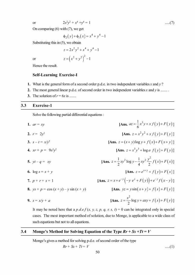
50
or 2x2y2 + x4 +y4 = 1 .....(7)On comparing (6) with (7), we get
4 42 1 1y x x y
Substituting this in (5), we obtain2 2 4 42 1z x y x y
or 22 2 1z x y
Hence the result.
Self-Learning Exercise-I
1. What is the general form of a second order p.d.e. in two independent variables x and y ?2. The most general linear p.d.e. of second order in two independent variables x and y is ....... .3. The solution of r = 6x is .......
3.3 Exercise-1
Solve the following partial differential equations :
1. ar = xy [Ans. 316
az x y x f y F y ]
2. r = 2y2 [Ans. 2 2z x y x f y F y ]
3. s – t = x/y2 [Ans. ( ) logz x y y f x F x y ]
4. xr + p = 9x2y2 [Ans. 3 3 logz x y a f y F y ]
5. yt – q = xy [Ans. 2
2 21 1log2 4 2
yz xy y xy f x F x ]
6. log s = x + y [Ans. x yz e f y F x ]
7. p + r + s = 1 [Ans. y y yz x e y e F y e f x y ]
8. ys + p = cos (x + y) – y sin (x + y) [Ans. sinyz y x y f x F y ]
9. s = x/y + a [Ans. 2
log2xz y axy f x F y ]
It may he noted here that a p.d.e.f (x, y, z, p, q, r, s, t) = 0 can he integrated only in specialcases. The most important method of solution, due to Monge, is applicable to a wide class ofsuch equations but not to all equations.
3.4 Monge’s Method for Solving Equation of the Type Rr + Ss +Tt = V
Monge’s gives a method for solving p.d.e. of second order of the typeRr + Ss + Tt = V .....(1)
51
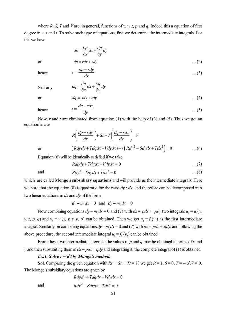
where R, S, T and V are, in general, functions of x, y, z, p and q. Indeed this a equation of firstdegree in r, s and t. To solve such type of equations, first we determine the intermediate integrals. Forthis we have
p pdp dx dyx y
or dp rdx sdy ....(2)
hencedp sdyr
dx
....(3)
Similarlyq qdq dx dyx y
or dq sdx tdy ....(4)
hencedq sdxt
dy
....(5)
Now, r and t are eliminated from equation (1) with the help of (3) and (5). Thus we get anequation in s as
dp sdy dq sdxR Ss T Vdx dy
or 2 2 0Rdpdy Tdqdx Vdydx s Rdy Sdydx Tdx ....(6)
Equation (6) will be identically satisfied if we take0Rdpdy Tdqdx Vdydx ....(7)
and 2 2 0Rdy Sdydx Tdx ....(8)
which are called Monge’s subsidiary equations and will provide us the intermediate integrals. Here
we note that the equation (8) is quadratic for the ratio dy : dx and therefore can be decomposed into
two linear equations in dx and dy of the form
1 0dy m dx and 2 0dy m dx
Now combining equations dy – m1dx = 0 and (7) with dz = pdx + qdy, two integrals u1 = u1(x,
y, z, p, q) and v1 = v1(x, y, z, p, q) can be obtained. Then we get u1 = f1(v1) as the first intermediate
integral. Similarly on combining equations dy – m2dx = 0 and (7) with dz = pdx + qdy, and following the
above procedure, the second intermediate integral u2 = f2 (v2) can be obtained.
From these two intermediate integrals, the values of p and q may be obtained in terms of x and
y and then substituting them in dz = pdx + qdy and integrating it, the complete integral of (1) is obtained.Ex.1. Solve r = a2t by Monge’s method.Sol. Comparing the given equation with Rr + Ss + Tt = V, we get R = 1, S = 0, T = – a2,V = 0.
The Monge’s subsidiary equations are given by0Rdpdy Tdqdx Vdydx
and 2 2 0Rdy Sdydx Tdx

52
Substituting the values of R, S, T and V, the subsidiary equations will be2 0dpdy a dqdx ....(9)
2 2 2 0dy a dx ....(10)Equation (10) may be factorised as
0dy adx ....(11)
and 0dy adx ....(12)Combining equation (11) with subsidiary equation (9), we get
2 0dp adx a dqdx
or 0dp adq (dx = 0, gives trivial solution) ....(13)Now from (11) and (13) we obtain
1y ax c , 2p aq c therefore the first intermediate integral is
1p aq f y ax ....(14)Similarly combining (dy + adx) = 0 with subsidiary equation (9), we get the second intermediate
integral as
2p aq f y ax ....(15)Now from above two intermediate integrals (14) and (15) we deduce the value of p and q as.
1 212
p f y ax f y ax
2 11
2q f y ax f y ax
a
Substituting these values of p and q in dz = pdx + qdy, we get
2 12 2dy adx dy adxdz f y ax f y ax
a a
On integration, we have
2 11 1
2 2 z y ax y ax
a aHence the required solution is
1 2z F y ax F y ax
Ex.2. Solve r + (a + b) s + abt = xy by Monge’s method.Sol. Comparing the given equation with Rr + Ss + Tt = V, we have R = 1, S = a + b,T = ab, V
= xy. Here Monge’s subsidiary equationsRdpdy + Tdqdx – Vdydx = 0Rdy2 – Sdxdy + Tdx2 = 0
become dpdy + abdqdx – xydxdy = 0 .....(16)and dy2 – (a + b) dxdy + ab dx2 = 0 .....(17)
53
Equation (17) may be factorised as(dy – bdx) = 0 .....(18)
and (dy – adx) = 0 .....(19)On integration y – bx = c1 .....(20)
y – ax = c2 .....(21)Combining equation (18) with subsidiary equation (16), we get
dp (bdx) + abdqdx – xydx (bdx) = 0or dp + adq – xy dx = 0or dp + adq – x (c1 + bx) dx = 0 [by using (20)]On integration, we get
2 3132 3
c bp aq x x c
or 2
332 3
x bp aq y bx x c
[by using (20)]
or 2 33
1 12 6
p aq yx bx c
Therefore the first intermediate integral is
2 31
1 12 6
p aq yx bx f y bx .....(22)
Similarly, the second intermediate integral corresponding to equation (19) is
2 32
1 12 6
p bq yx ax f y ax .....(23)
Now from above two intermediate integrals (22) and (23), we deduce the values of p and q as
2 32 1
1 1 12 6
p x y a b x a f y ax b f y bxa b
and 31 2
1 16
q x f y bx f y axa b
Substituting these values of p and q in dz = pdx + qdy, we get
2 32 1
31 2
1 1 12 6
1 16
dz x ydx a b x dx af y ax dx bf y bx dxa b
x dy f y bx dy f y ax dya b
or
2 3 32 1
1 2
1 1 136 6
1
dz x ydx x dy a b x dx af y ax dx bf y bx dxb a
f y bx dy f y ax dyb a
54
or
3 32
1
1 1 16 6
1
dz d x y a b x dx f y ax dy adxb a
f y bx dy bdxb a
Integrating, we get the required solution as
3 41
1 16 24
z x y a b x y ax y bx
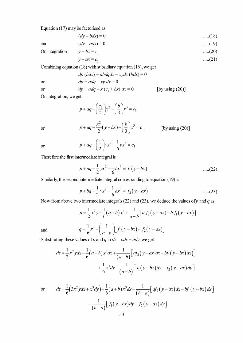
Ex.3. Solve x2r + 2xy s + y2t = 0 by Monge’s method.Sol. Comparing the given equation with Rr + Ss + Tt = V, we have R = x2, S = 2xy, T = y2,
and V = 0. Hence Monge’s subsidiary equations0Rdpdy Tdqdx Vdydx
2 2 0Rdy Sdx dy Tdx become
2 2 0x dpdy y dqdx .....(24)
and 2 2 2 22 0x dy xy dy y dx .....(25)Equation (25) may be factorised as
2 0xdy ydx
or 0xdy ydx .....(26)
Combining it with the equation (24), we getxdp (ydx) + y2dq dx = 0
or xdp + ydq = 0or xdp + pdx + qdy + ydq = pdx + qdyor d (xp) + d (yq) = dzOn integration, we get
px + qy = z + c1
Now equation (26) gives
2y cx
Thus the intermediate integral will bepx + qy = z + f (c2)
which is of Lagrange’s form having the subsidiary equations
2
dx dy dzx y z f c
First two terms gives
2y cx
and the last two terms gives 2z f c cy

55
Hence required solution is
1 2y yz yf fz x
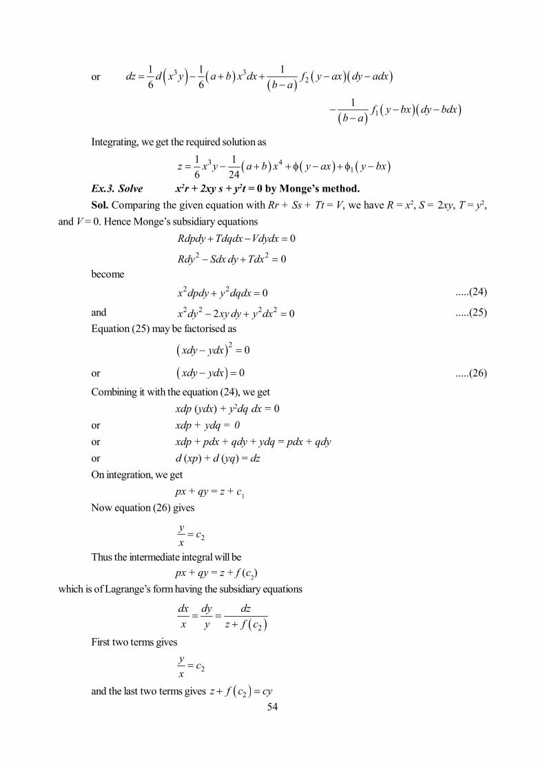
Ex.4. Solve (x – y) (xr – xs – ys – yt) = (x + y) (p – q) by Monge’s method.Sol. Monge’s subsidiary equations in this case will be
0x x y dpdy y x y dqdx x y p q dxdy .....(27)
and 2 2 0x dy x y dxdy y dx .....(28)
Factors of equation (28) arexdy + ydx = 0,
which on integration gives xy = c1
and dx + dy = 0,which on integration gives x + y = c2 . Combining equation (27) with (xdy + ydx) = 0, we get
x y dp dq p q dx dy
On integration, we obtain
constant.p qx y
Therefore the intermediate integral is(p – q) = (x – y) f (xy)
for which the Lagrange’s subsidiary equation will be
1 1 0f xy ydx xdy dzdx dy dz
x y f xy
From first two terms, we getFrom the last two relations, we get x + y = c2
dz + f (xy) d (xy) = 0On integration
z = F1 (xy) + constantHence required solution is
z = F1 (xy) + F2 (x + y)Ex.5. Solve q2r – 2pqs + p2t = 0 by Monge’s method.Sol. Monge’s subsidiary equations in this case will be
q2 dpdy + p2dqdx=0 .....(29)and 2 2 2 22 0q dy pq dx dy p dx .....(30)Factors of equation (30) are
2 0qdy pdx
or 0qdy pdx
which on integration gives (after putting in dz = pdx + qdy)
dz = 0 1 constantz c

56
Now substituting qdy = – pdx in (29), we get
2 0qdp pdx p dqdx
or qdp – pdq = 0 [dx = 0 will give the trivial solution]On integration, we get
constantp bq
Therefore the intermediate integral is
p f zq
or 0p q f z
For which the Lagrange’s subsidiary equation will be
1 0dx dy dz
f z
from first two terms, we get
y x f z c
and from last two terms, we getz = c1
Hence the required solution is y x f z F z as c = F (z)
Ex.6. Solve t – r sec4y = 2q tan y by Monge’s method.Sol. Monge’s subsidiary equations in this case will be
4sec 2 tan 0ydpdy dqdx q y dxdy .....(31)
and 4 2 2sec 0y dy dx .....(32)
Factors of equation (32) aredx – sec2y dy = 0, .....(33)
which on integration gives x – tan y = constantand dx + sec2y dy = 0 .....(34)
which on integration givesx + tan y = constant
Now combining (34) with equation (31), we get2sec 2 tan 0y dp dq q y dy
On integration, we get
21cos constant tanp q y f x y .....(35)
Similarly, when (33) is combined with (31) , and integrated gives
22cos tanp q y f x y .....(36)

57
On solving (35) and (36), we get the values of p and q as
1 21 tan tan2
p f x y f x y
21 2
1 sec tan tan2
q y f x y f x y
Substituting these values in dz = pdx + qdy, we obtain
21 2 1 2
1 1tan tan tan tan sec2 2
dz f x y f x y dx f x y f x y y dy
or 2 21 22 tan sec tan secdz f x y dx y dy f x y dx y dy
which on integration gives the required solution as
1 22 tan tanz F x y F x y
3.5 Monge’s Method for Solving Equation of the Type Rr + Ss + Tt + U (rt – s2) = V
Prof G. Monge gave a method for solving equationRr + Ss + Tt + U (rt – s2) = V .....(1)
where R, S, T, U and V are, in general, functions of x, y, z, p and q.We know that
p pdp dx dyx y
or dp rdx sdy
ordp sdyr
dx
.....(2)
Similarlyq qdq dx dyx y
thereforedq Sdxt
dy
......(3)
Putting the values of r and t from (2) and (3) in (1), we get
2
dp sdy dq sdx dp sdy dq sdxR Ss T U s Vdx dy dx dy
or (Rdpdy + Tdqdx + Udpdq – Vdxdy) – s (Rdy2 – Sdxdy + Tdx2
+ Udpdx + Udqdy) = 0 .....(4)Equation (4) will be identically satisfied if we take
Rdpdy + Tdqdx + Udpdq – Vdxdy = 0 .....(5)
and 2 2 0Rdy S dxdy Tdx Udpdx Udqdy .....(6)
These simultaneous equations (5) and (6) are known as Monge’s subsidiary equations.Here the equation (6) can not be factorized. So we will try to factorize

58
2 2
0
Rdy S dxdy Tdx Udpdx Udqdy
Rdpdy Tdq dx Udpdq Vdxdy
.....(7)
where is some multiple and is determined later.Let us suppose that the factors of (7) are
1 21 2
1 0Rdy m Tdx m Udp dy dx dqm m
.....(8)
On comparing (7) with (8), we obtain
11
,R m T S Vm
2 1m m , 2
R Um .....(9)
The last two relations gives 1RmU
. Putting this in the first relation of (9), we obtain
2 2 0 UV RT SU U .....(10)
This equation is called –equation, where , in general, is a function of x, y, z, p and q.Now since equation (10) is quadratic in so suppose that it is satisfied by two values of say
1 and 2 then the factors corresponding to these values will be
11
10R U URdy Tdx R dp dy dx dq
U R R
as 11 2
Rm mU
or 1 1 1 1 0Udy Tdx Udp Udx Rdy Udq .....(11)
Similarly corresponding to 2, we can obtain
2 2 2 2 0Udy Tdx Udp Udx Rdy Udq .....(12)
Now one factor from (11) and one from (12) will be combined in pairs to get intermediate inte-grals in the form u = f (v). We can combine factors as
1 1 0Udy Tdx Udp
2 2 0Udx Rdy Udp
and 1 1 0Udx Rdy Udp
2 2 0Udy Tdx Udp
These two pairs will give intermediate integrals provided these total differential equations areintegrable, from which the values of p and q can be determined. Substituting these values of p and q indz = pdx + qdy, we get the general solution on integration.
Ex.1. Solve 3r + 4s + t + (rt – s2) = 1Sol. Comparing the given equation with Rr + Ss + Tt + U (rt – S2) = V, we have R = 3, S = 4,
T = 1, U = 1, V = 1. Then – quadratic equation

59
2 2 0UV RT SU U
becomes 24 4 1 0
or 21 2
12 1 02
Hence there is only one intermediate integral given by the equations
1 1 0Udy Tdx Udp
and 2 2 0Udx Rdy Udq
On putting above values, we get
1 1 02 2
dy dx dp
and1 13 02 2
dx dy dq
or 2 0dy dx dp
and 3 2 0dy dx dq On integration, we obtain
12y x p c .....(13)
and 23 2y x q c .....(14)Hence the only intermediate integral is
2 3 2y x p f y x q
where f is any arbitrary functionNow solving (13) and (14) for p and q, we get
12p y x c
23 2q y x c
Putting these values of p and q in dz = pdx + qdy, we get
1 22 3 2dz y x c dx y x c dy
or 1 22 3dz ydx xdy xdx ydy c dx c dy
On integrating, we obtain the general solution as
2 21 2 3
1 322 2
z xy x y c x c y c
where c1, c2, c3 are arbitrary constants.Ex.2. Solve 2s + (rt – s2) = 1Sol. Comparing the given equation with Rr + Ss + Tt + U (rt – S2) = V, we have R = 0, S = 2,
T = 0, U = 1, V = 1.Then the quadratic equation
2 2 0UV RT SU U
becomes 2 2 1 0
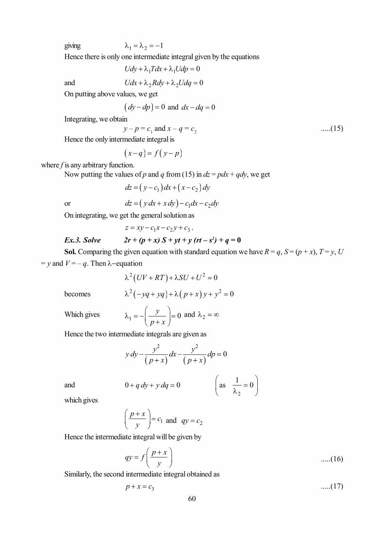
60
giving 1 2 1 Hence there is only one intermediate integral given by the equations
1 1 0Udy Tdx Udp
and 2 2 0Udx Rdy Udq On putting above values, we get
0dy dp and 0dx dq
Integrating, we obtainy – p = c1 and x – q = c2 .....(15)
Hence the only intermediate integral is
x q f y p where f is any arbitrary function.
Now putting the values of p and q from (15) in dz = pdx + qdy, we get
1 2dz y c dx x c dy
or 1 2dz y dx x dy c dx c dy
On integrating, we get the general solution as
1 2 3z xy c x c y c .Ex.3. Solve 2r + (p + x) S + yt + y (rt – s2) + q = 0Sol. Comparing the given equation with standard equation we have R = q, S = (p + x), T = y, U
= y and V = – q. Then equation
2 2 0UV RT SU U
becomes 2 2 0yq yq p x y y
Which gives 1 0yp x
and 2
Hence the two intermediate integrals are given as
2 2
0y yy dy dx dpp x p x
and 0 0q dy y dq 2
1as 0
which gives
1p x c
y
and 2qy c
Hence the intermediate integral will be given by
p xqy fy
.....(16)
Similarly, the second intermediate integral obtained as
3p x c .....(17)
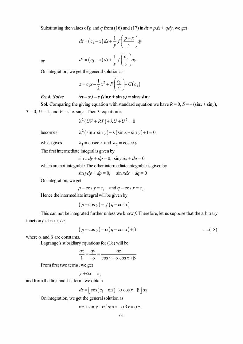
61
Substituting the values of p and q from (16) and (17) in dz = pdx + qdy, we get
31 p xdz c x dx f dyy y
or 33
1
cdz c x dx f dyy y
On integration, we get the general solution as
2 33 3
12
cz c x x F G cy
Ex.4. Solve (rt – s2) – s (sinx + sin y) = sinx sinySol. Comparing the giving equation with standard equation we have R = 0, S = – (sinx + siny),
T = 0, U = 1, and V = sinx siny. Then -equation is
2 2 0UV RT U U
becomes 2 sin sin sin sin 1 0x y x y
which gives 1 cosce x and 2 cosce y
The first intermediate integral is given bysin x dy + dp = 0, siny dx + dq = 0
which are not integrable.The other intermediate integrable is given bysin ydy + dp = 0, sin xdx + dq = 0
On integration, we getp – cos y = c1 and q – cos x = c2
Hence the intermediate integral will be given by
cos cosp y f q x
This can not be integrated further unless we know f. Therefore, let us suppose that the arbitraryfunction f is linear, i.e.,
cos cosp y q x .....(18)where and are constants.
Lagrange’s subsidiary equations for (18) will be
1 cos cosdx dy dz
y x
From first two terms, we get
3y x c and from the first and last term, we obtain
3cos cosdz c x x dx On integration, we get the general solution as
24sin sinz y x x c

62
Ex.5. Solve z (1 + q2) r – 2pqzs (1 + p2) t + z2 (rt – s2) + 1 + p2 + q2 = 0Sol. Comparing the given equation with the standard equation, we have R = z (1 + q2),
S = – 2pqz, 2 21 ,T p U z and 2 21V p q . Then the -equation is
2 2 2 22 0p q pqz z
or 2 0pq z
which gives zpq
Putting the value of in0Udy T dx U dp
and 0U dx R dy U dq we getand pqdy + (1 + p2) dx + zdp = 0 .....(19)
pqdx + (1 + q2) dy + zdp = 0 .....(20)dz p dx q dy .....(21)
Combining (19) and (21), and on integration, we obtainx + zp = c1 .....(22)
Similarly by combining (20) and (21), and on integration, we obtainy + zq = c2 .....(23)
Putting the values of p and q obtained from (22) and (23) in dz = p dx + qdy, we get
1 2c x c ydz dx dyz z
Integrating 2 221 2 3cz c x y c
which is the required solution.Ex.6. Solve 5r + 6s + 3t + 2 (rt – s2) + 3 = 0Sol. Comparing the given equation with the standard equation, we have R = 5, S = 6, U = 2,
and V = – 3. Then the equation will be29 12 4 0
or 23 2 0
which gives 1 223
There is only one intermediate integral given by the equations
2 22 3 2 03 3
dy dx dp
and2 22 5 2 03 3
dx dy dq
or 3 3 2 0dy dx dp

63
and 3 5 2 0dx dy dq
Integrating,we get 3y – 3x – 2p = c1 .....(24)and 3x – 5y – 2q = c2 .....(25)Hence the only intermediate integral is
3y – 3x – 2p = f (3x – 5y – 2q) .....(26)where f is an arbitrary function.
Solving (24) and (25) for p and q, we get
11 3 32
p y x c and 21 3 52
q x y c
Putting p and q in dz = p dx + q dy, we get
1 21 13 3 3 52 2
dz y x c dx x y c dy
or 2dz = 3 (ydx + xdy) – 3xdx – 5ydy – c1dx – c2dyIntegrating, we get
2 21 2 3
3 52 32 2
z xy x y c x c y c
which is the required solution. c1, c2 and c3 are arbitrary constants.
Self-Learning Exercise-II
1. For p.d.e. R r + Ss + Tt = V1 the Monge’s subsidiary equations are ................ and ..... .... ...
2. The Monge’s subsidiary equations for p.d.e. r = kt are .... ..... and ..... ..... .3. The -equation in Monge’s method for solving p.d.e. r + 3s + t + (rt – s2) = 1 is .... .... ....
3.6 Summary
In this unit, you learn about partial differential equations of second order and their solution. Youalso studied the solution of two types of P.D.E. by Monge’s method.
3.7 Answers of Self–Learning Exercise
Exercise-I
1. , , , , , , , 0F x y z p q r s t
2. Rr Ss Tt Pp Qq Zz F
3. 3z x x f y y
Exercise-II
1. 0R dpdy T dq dx V dy dx 2 2 0R dy S dy dx Tdx

64
2. 0dp dy R dq dx and 2 2 0dy r dx
3. 22 3 1 0
3.8 Exercise-II
Solve the following P.D.E by Monge’s method :1. pt – qs = q3 [Ans. y = xz + f (z) + F (x)]2. y2r – 2ys + t = p + 6y [Ans. z = y3 – y f (y2 + 2x) + F (y2 +2x)]
3. 2 22 5 2 2 0x r xys y t px qy [Ans. z = f (x2 y) + F (xy2)]
4. 2 21 2 1 1 0q r p q pq s p t [Ans. y = f (x + y + z) + x F (x + y + z)]
5. (q + 1) s = (p + 1) t [Ans. z = f(x) +(x + y + z) or y – (x + y + z = (x)]6. r – t cos2 x + p tan x = 0 [Ans. 2z = f (y + sin x) – F (y – sin x)]7. s2 – rt = a2 [Ans. z = x f1 (q – ax) + qy + (q – ax)]8. ar + bs + ct + e (rt – s2) = b, where a, b, c, e, and h are constants
2 2
1 2 constant2 2x ayez xf ay eq m x y ay eq
Ans.
9. 2 pr + 2qt – 4pq (rt – s2) = 1 3 2 3 21 2 33 2 2z c x c y c Ans.
Solve the following partial differential equations :10. 2r + tex – (rt – s2) = 2ex [Ans. z = ex + bx + y2 – ay + c]
11. 3r + s + t + (rt – s2) + 9 = 0 2 232 5
2 2x yz cy xy f c x F c
Ans.
12. r + 3s + t + (rt – s2) = 1 21 2 2 1
12
z x y F F f f Ans.
13. (rt – s2) + 3s = 2 1 ; ;2
x y f g z xy y Ans.
14. qxr+(x + y)s + pyt + xy(rt – s2)=1 – pq 1 log mz y mx n x f x ym
Ans.

65
Unit 4 : Classification of Linear PDE of Second Order,Cauchy Problem and Method of Separationof Variables
Structure of the Unit
4.0 Objective
4.1 Introduction
4.2 Classification of PDE of Second Order
4.3 Classification of Second Order PDE in More Than Two Independent Variables
4.4 Cauchy Problem
4.5 Method of Separation of Variables
4.6 Summary
4.7 Answers to Self-Learning Exercises
4.8 Exercise
4.0 Objective
Partial differential equations generally occur in the problems of physics and engineering. Afterstudying this unit, you should be able to identify and classify partial differential equations (PDE). You willhave an idea of Cauchy problem. At last you will get knowledge of how to solve the partial differentialequations by method of separation of variables.
4.1 Introduction
The importance of partial differential equations among the topis of applied mathematics has beenrecognized for many years. However, the increasing complexity of today’s technology is demanding of themathematician, the engineer and the scientists, an understanding of the subject previously attained only byspecialists. This unit of partial differential equations (PDE) comprises identification and classification ofPDE. It also presents the principal technique method of separation of variables for constructing solution topartial differential equation problems. The solved and supplementary problems have the vital role of apply-ing reinforcing and sometimes expanding the theoretical concepts.
4.2 Classification of PDE of Second Order
Consider the second order partial differential equationRr + Ss + Tt + f (x, y, z, p, q) = 0 ....(1)

66
where R, S and T are continuous functions of x and y only possessing continuous partial derivatives. ThePDE can be classified into three categories depending on nature of values of the discriminant S2 – 4RT.Thus (1) is known as
(i) Hyperbolic if S2 – 4RT > 0(ii) Parabolic if S2 – 4RT = 0(iii) Elliptic if S2 – 4RT < 0
Ex. 1 : Consider the one dimensional Laplace’s equation 2
2
2
2z z
x y
= 0 i.e. r + t = 0. Compar--
ing it with equation (1), we have R = 1, S = T = 0. Hence S2 – 4RT = 0 and so given equation is parabolic.
Ex. 2 : Consider the one dimensional diffusion equation 2
2z z
yx
i.e. r – q = 0. Comparing it
with equation (1), we have R = 1, S = 0 and T = – 1. Hence S2 – 4RT = 4 > 0 and so given equation ishyperbolic.
4.3 Classification of a Second Order PDE in More Than Two Independent Variables
A linear second order partial differential equation having more than two independent variables cansuitably be reduced, in general, to a canonical form only when the coefficients are constants. Let x, x2,...,xn be n independent variables and u be the dependent variable, then such a second order PDE may bewritten as
2
1 1 10
n n n
ij ii j ii j j
u ua b cux x x ....(1)
where aij, bi and c are constants and aij = aji. Now we consider a one-one transformationi = i (x1, x2, ....., xn), i = 1, 2, ....., n ....(2)
Then the equation (1) transforms to
1 21 21 1
, ,...., ; , , ,..., 0k l n
n nkl n
k lA u F u u u u
.....(3)
where i j
kl ij k ix xA a ...(4)
The characteristic quadratic Q() associated with equation (1) in this case is
Q() = 1 1
n nij i j
i ja
...(5)
The associated real symmetric matrix in this case will be
11 12 1
21 22 2
1 2
.....
.....
.....
n
n
n n nn
a a aa a aM
a a a
....(6)

67
and the characteristic roots “eigenvalues” will be given by | M – | = 0 ...(7)
and their nature and signs will determine the type of the given PDE.Case I : Elliptic PDE : If all the eigenvalues are nonzero and of the same sign, the given PDE is
of elliptic type.Case II : Hyperbolic PDE : If all the eigenvalues are nonzero and have the same sign except
precisely one of them, the given PDE is of hyperbolic type.Case III : Ultra Hyperbolic PDE (n 4) : If all the eigenvalues are nonzero and atleast two of
them are positive and two negative then the given PDE is of ultra hyperbolic type.Case IV : Parabolic PDE : If any of the eigenvalues is zero, the given PDE is of parabolic type.Note : As an alternative of finding the eigenvalues of matrix M, which sometimes may be cumber
-some, the classification can be made with the help of by expressing the quadratic form (5) as a sum ofsquares. The number of positive and negative squares will be the same as the number of positive andnegative eigenvalues of the associated matrix. Either of the methods, as per convenience, may be chosenfor the classification of partial differential equation.
Ex. 1. Determine the nature of following PDE
22 2
2 2z z= x
x y
Sol.2 0
y
2 2
2 2z zx
x
Comparing with standard second order PDE, we haveR = 1, S = 0, T = – x2
S2 – 4RT = 0 – 4 (–x2) = 4x2
Since x2 > 0, therefore given PDE is hyperbolic.Ex. 2. Classify the following PDE as hyperbolic, parabolic or elliptic :
022 2 2
2 2z z z
x yx y
Sol. On comparing it with equation (1), we haveR = 1, S = 2, T = 1
Hence the value of discriminant S2 – 4RT = 0Therefore given PDE is parabolic in nature.
Ex. 3. Find the nature of following PDE
3 2 5 = 02 2 2
2 2z z z z
xx y yx y
Sol. On comparing given equation with standard PDE, we haveR = 3, S = 2, T = 5
So S2 – 4RT = 1 – 15 = – 14 < 0then given PDE is elliptic in nature.

68
Ex. 4. Show that the equation 2 2 2
22 2 22 1 0z z zx y
x x y y
is elliptic for values of x and in the region x2 + y2 < 1, parabolic on the boundaryand hyperbolic outside this region.
Sol. Given equation is
2 2 2
22 2+ 2 + 1 = 0
z z zx yx yx y
Obviously R = 1, S = 2x, T = 1 – y2
Now discriminant isS2 – 4RT = 4x2 – 4(1 – y2) = 4(x2 + y2 – 1)
Given equation is elliptic in nature ifS2 – 4RT < 0
or 4(x2 + y2 – 1) < 0 x2 + y2 < 1 (inside boundary)Given equation is parabolic in nature if
S2 – 4RT = 0or 4(x2 + y2 – 1) = 0 x2 + y2 = 1 (on boundary)
Given equation is hyperbolic in nature ifS2 – 4RT >0
or 4(x2 + y2 – 1) > 0 x2 + y2 > 1 (outside the boundary)Ex. 5. Classify the following differential equation as to type in the second quadrant
of xy-plane
2 02 2 2
2 2 2 22 2u u u
y x x y y xx yx y
Sol. : Here 2 2R y x , 2S x y , 2 2T y x
Now S2– 4RT = 4(x – y)2 – 4(x2 – y2) = 4(x2 + y2 – 2xy – y2 – x2) = – 8xy
In second quadrant, y is positive while x is – negative,thereforeS2 – 4RT = +ve > 0
Hence given PDE is hyperbolic in nature.Ex. 6. Classify the equations :
(a)2 2 2 2 2
2 2 22 2 2 u u u u u
x y y zx y z
(b)2 2 2 2
2 2 2 2 21u u u u
+ + = x y z c t
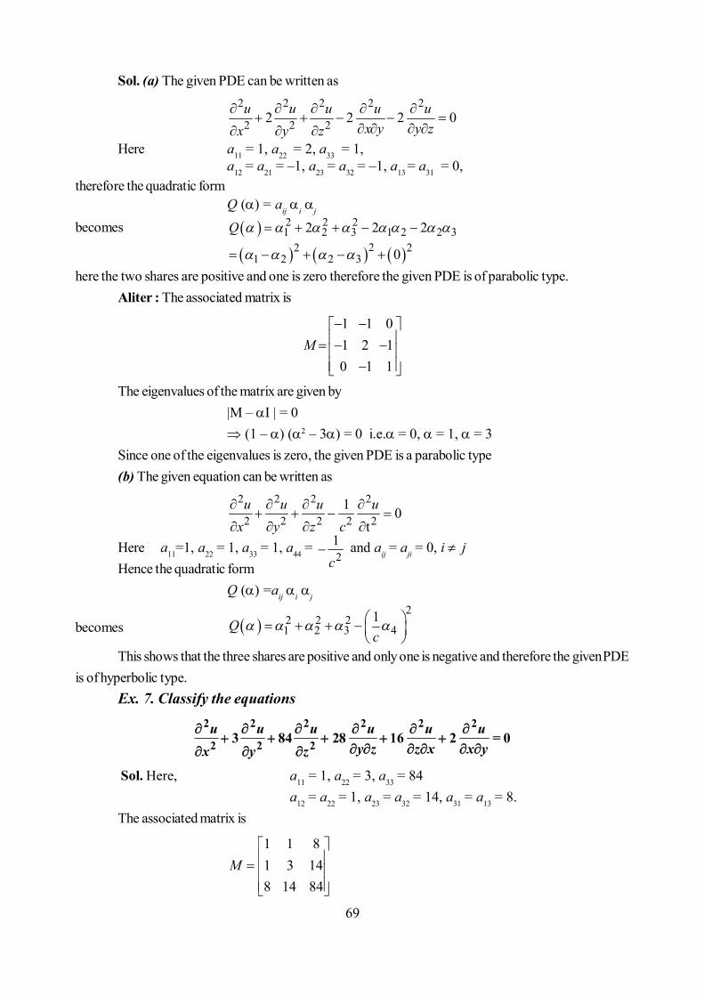
69
Sol. (a) The given PDE can be written as2 2 2 2 2
2 2 22 2 2 0u u u u ux y y zx y z
Here a11 = 1, a22 = 2, a33 = 1,a12 = a21 = –1, a23 = a32 = –1, a13 = a31 = 0,
therefore the quadratic formQ () = aij i j
becomes 2 2 21 2 3 1 2 2 32 2 2Q
22 21 2 2 3 0
here the two shares are positive and one is zero therefore the given PDE is of parabolic type.Aliter : The associated matrix is
1 1 01 2 10 1 1
M
The eigenvalues of the matrix are given by|M – I | = 0(1 – ) ( – 3) = 0 i.e.= 0, = 1, = 3
Since one of the eigenvalues is zero, the given PDE is a parabolic type(b) The given equation can be written as
2 2 2 2
2 2 2 2 21 0
tu u u u
x y z c
Here a11=1, a22 = 1, a33 = 1, a44 = 21
c and aij = aji = 0, i j
Hence the quadratic formQ () =aij i j
becomes 2
2 2 21 2 3 4
1Qc
This shows that the three shares are positive and only one is negative and therefore the given PDEis of hyperbolic type.
Ex. 7. Classify the equations2 2 2 2 2 2
2 2 23 84 28 16 2 = 0u u u u u u
y z z x x yx y z
Sol. Here, a11 = 1, a22 = 3, a33 = 84a12 = a22 = 1, a23 = a32 = 14, a31 = a13 = 8.
The associated matrix is
1 1 81 3 148 14 84
M

70
The eigenvalues of the matrix are given by
| M – I | = 0
– 98+ 78 – 4 = 0By Descarte’s rule of signs, The given equation has all the three positive roots and therefore the
given PDE is of elliptic type.Aliter : The quadratic form
Q () = aij i j
becomes Q() = 2 2 21 2 3 1 2 1 3 2 33 84 2 16 28
22 21 2 3 2 3 38 2 3 2
Here all the three squares are positive the given PDE is of elliptic type.
Self -Learning Exercise–11. Mark the correct alternative :
(i) The second order PDE Rr +Ss +Tt +f (x, y, z, p, q) = 0 is parabolic if(a) S2 – 4RT > 0 (b) S2 – 4RT = 0 (c) S2 – 4RT < 0 (d) none of these
(ii)The PDE 2 2 2
2 2+ + = 0u u u
x yx y
is
(a) hyperbolic (b) parabolic (c) elliptic (d) none of these
(iii) In the region x2 > 4y the PDE 2 2 2
2 2+ + = 0u u u
x yx yx y
is
(a) hyperbolic (b) parabolic (c) elliptic (d) none of these
(iv) The differential equation 2 2 2
2 24 16 + 9 = 0u u u
x yx y
is
(a) hyperbolic (b) parabolic (c) elliptic (d) none of these2. Write the condition under which a second order PDE in more than two independent variables is
elliptic.3. The region in which the equation (x log y) r + 4yt = 0 is hyperbolic is...
4. Classify the following PDE 2 2 2
2 24 + 4 + = 0u u u
x yx y
5. Classify the PDE 2 2 2
2 25 9 + 4 = 0u u u
x yx y
6. Classify the PDE 2 2 2
2 2+ + + 2 + + 6 = 0u u u u ut x ux t t xt x

71
4.4 Cauchy Problem
The Cauchy problem is a boundary value problem dealing with the unique solution of a secondorder quasi–linear PDE when its initial value and slope are specified.
Statement : Determine the solution z = z(x, y) of the PDERr + Ss + Tt + f(x, y, z, p, q) = 0 ...(1)
where R, S and T are in general functions of x, y, z, p and q such that the solution takes on a givenspace curve C, having the parametric equation
x = x(t), y = y(t), z = z(t) ...(2)
prescribed value of z and zn
, where n is the distance measured along the normal to the curve.
The latter set of boundary conditions is equivalent to assuming that the values of x,y, z, p, q aredetermined on the curve, but it be noted that the values of p and q can not be assigned arbitrarily along thecurve.
Method of solution : The solution of eq. (1) will be some surface, called integral surface,passing through C. Hence at each point of C, by relations (2) we have
0 0z px qy .....(3)which shows that p0 and q0 are not independent.
Thus, the Cauchy problem finds the solution of (1) passing through the integral strip of the firstorder formed by the planar elements (x0,y0, z0, p0, q0) of the curve C. At every point of the integral stripp0 = p0(t), q0 = q0(t), so that of we differentiate these equation w.r.t. ‘t’ we find that
0 0 0 0 0 0,p rx sy q sx ty ....(4)
Knowing R, S, T, f, 0 0 0 0 0 0, , , , ,x y p q p q at each point of C, we may regard equations (1) and(4) as linear simultaneous equations for the unknowns r, s, t at each point of C. Solving by Cramer’s’s rule,we get
1 2 3
1r s t
.....(5)
where 1 0 0
0 0 0
0S T fy px y q
, 2 0 0
0 0
00
R T fx p
y q
3 0 0 0
0 00
R S fx y p
x q
.....(6)
0 0
0 0
00
R S Tx y
x y
.....(7)

72
If 0, we can easily calculate the expressions for second order derivatives r0, s0 and t0 along C.The third order partial differential coefficient of z can similarly be calculated at every point of C by
differentiating (1) w.r.t. x and y respectively, making use of
0 0 0xxx xxyr z x z y .....(8)etc. and solving as above.
Proceeding in this manner, we can calculate partial derivatives of every order of the points of C.The values of the function z at neighbouring points, can be obtained by using Taylor’s Theorem for func-tions of two independent variables. Thus the Cauchy problem possesses a solution as long as 0. In the elliptic case 4RT – S2 > 0, so that 0 always holds and the derivatives, of all orders, of zare uniquely determined.
If = 0, then the Cauchy’s method of solution breaks down. This critical case leads to thecondition
2 2 0Ry Sxy Tx
or 2 2 0Rdy Sdydx Tdx ....(9)At each point (x,y, 0) of (which is orthogonal projection of the curve C on the plane z = 0) the
eq. (9) would give a pair of directions along which = 0. These directions are called as characteristics.Thus curves known as characteristic base curves, may be drawn through every point (x,y, 0) of
the base curve simply by approximating them by straight line segments whose directions are taken tocoincide with those of the tangents given by the roots of (9), viz.
2 42
dy S S RTdx R
.....(10)
Thus a curve in the xy plane satisfying (10) is called a characteristic base curve of the PDE (1),and the curve C of which it is the projection is called a characteristics curve of the same equation.
Note that characteristics are :(i) Real and distinct if S 2 – 4RT > 0(ii) Coincident if S2 – 4RT = 0 and(iii) Imaginary if S2 – 4RT < 0Hence these are two families of characteristics if the given PDE is hyperbolic, one family if it is
parabolic and none if it is elliptic. Thus the Cauchy problem will fail to have unique solution if an arc elementof the base curve coincides with the characteristics. Consequently, the condition 0 is both necessaryand sufficient to solve the Cauchy problem.7
Characteristic equations :Corresponding to (1), consider –quadratic
R2 + S + T = 0 ....(11)when S2 – 4RT 0, eq. (11) has real roots. Then, the ordinary differential equation
, 0dy x ydx
are called the characteristic equations.Again the solution of (11) will be characteristic curves or simply the characteristic of the second
order PDE (1).

73
4.5 Method of Separation of Variables
For given linear second order partial differential equationRr +Ss +Tt +Pp +Qq +Zz = F (x,y) ....(1)
where R, S, T, P, Q, Z and F are functions of independent variables x and y only. Let Z(x,y) be solution of(1).
The method of separation of variables for this problem is a powerful tool and begins with assump-tion that Z(x,y) is of the form X(x) . Y(y) i.e.
Z(x,y) = X(x) .Y(y) ....(2)where X is function of independent variables x only and Y is function of independent variables y only.
On substituting (2) in (1) we have
1 1f D X = g D YX Y
....(3)
where f (D) and g(D) are quadratic functions of D =x
and D =y
respectively. This has the effect of
replacing the single PDE with two second order linear ordinary differential equations since LHS of (3) isfunction of x alone and the RHS is function of y alone. Since x and y are independent variables, the twosides of (3) will be equal only if each side is a constant (say ) be
1 1 f D X g D YX Y
or and f D X X g D Y Y .....(4)
which can be solved by the methods of ordinary differential equation.The theory of eigenfunction expansions enters into the treatment of any in homogenous aspect of
the problem. The general solution of equation (4) will depend on the choice of positive or negative orzero. In practical problems, the nature of the boundary conditions determine the nature of and itbecomes an eigenvalue problem.
The method of separation of variables can be employed in a similar manner for more than twoindependent variables also.
In the application of ordinary linear differential equation, we first find the general solution and thendetermine the arbitrary constant from the initial values, But the same method is not applicable to probleminvolving PDE In method of separation of variables right from the beginning we try to find the particularsolution of PDE which satisfy all or some of the boundary conditions and then the remaining conditions arealso satisfied. The combination of these particular solutions gives the solution of the problem.
Ex. 1. Find the characteristics ofy2r – x2t = 0.
Sol. Given y2r – x2t = 0 ....(5)Comparing (5) with
Rr + Ss + Tt + f (x, y, z, p, q) = 0, we have .....(6)
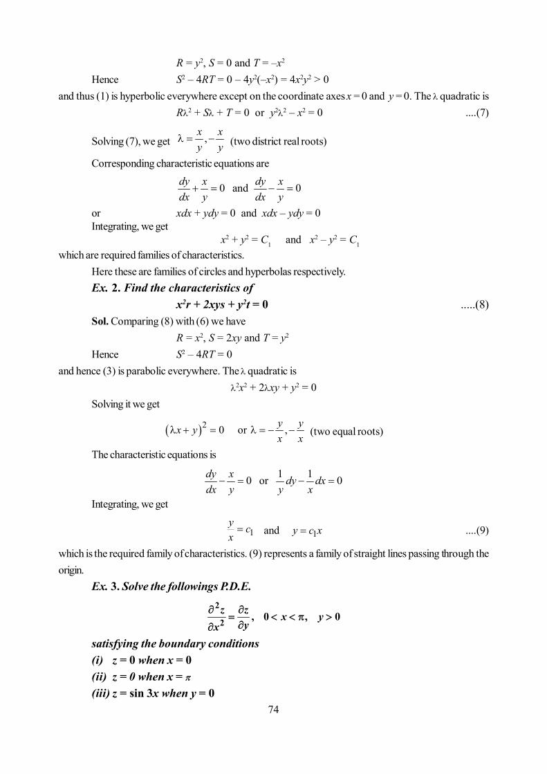
74
R = y2, S = 0 and T = –x2
Hence S2 – 4RT = 0 – 4y2(–x2) = 4x2y2 > 0and thus (1) is hyperbolic everywhere except on the coordinate axes x = 0 and y = 0. The quadratic is
R2 + S + T = 0 or y22 – x2 = 0 ....(7)
Solving (7), we get ,x xy y
(two district real roots)
Corresponding characteristic equations are
0 and 0dy x dy xdx y dx y
or xdx + ydy = 0 and xdx – ydy = 0Integrating, we get
x2 + y2 = C1 and x2 – y2 = C1
which are required families of characteristics.Here these are families of circles and hyperbolas respectively.Ex. 2. Find the characteristics of
x2r + 2xys + y2t = 0 .....(8)Sol. Comparing (8) with (6) we have
R = x2, S = 2xy and T = y2
Hence S2 – 4RT = 0and hence (3) is parabolic everywhere. The quadratic is
2x2 + 2xy + y2 = 0Solving it we get
2 0 or ,y yx yx x
(two equal roots)
The characteristic equations is
1 10 or 0dy x dy dxdx y y x
Integrating, we get
1y cx and 1y c x ....(9)
which is the required family of characteristics. (9) represents a family of straight lines passing through theorigin.
Ex. 3. Solve the followings P.D.E.2
2 , 0 , 0z z x yyx
satisfying the boundary conditions(i) z = 0 when x = 0(ii) z = 0 when x = (iii) z = sin 3x when y = 0

75
Sol. Let z(x, y) be solution of given PDE Assume thatz(x, y) = X(x)Y(y)
where X and Y be function of only x and y respectively.On substituting the value of z(x, y) = X(x)Y(y) in given PDE, we have
2
22
1 1 sayd X dY nX Y dydx
then2
2 22 0, 0d X dYn X n Y
dydx
Hence sin ,X a nx and2n yy be
where a, b, are arbitrary constants
Thus z = X(x)Y(y) = 2
sin n yA nx e , A = ab .....(10)
According to conditions (i) and (ii) given with the problem, from (10), we get2
0 sin n yA e and 2
0 1 sin .n n yA e Thus = 0 as A 0
Hence 2sin n yz A nx e .....(11)
Also by condition (iii), from (11), we get sin 3x = A sin nx A= 1, n = 3
Hence 9sin 3 yz xebe required solution of given PDE under specified boundary conditions.
Ex. 4. Use the method of separation of variables to solve the equation
32 ,0 6 xu u u given that u x ex t
Sol. Let u(x, t) = X(x)T(t) be solution of given PDE where X is a function of x only and T is a
function of t only.
Nowu dX u dTT and Xx dx t dt
On substituting these values in given PDE, we get
2dX dTT X XTdx dt
Dividing by XT, we have
22 1X T nX T (say)
Now we have two ordinary differential equations.
2 22and 1X Tn nX T
or2
2 10,2
T ndX n X andTdx

76
Sloving these equations, we find that2
21
21 2and
n tn xX c e T c e
Hence
22 1
21 2,
nn x tu x t X x T t c c e
Under given condition we get 23
1 26 x n xe c c e
c1c2 = 6 and n2 = 3Thus the required solution of the problem is u(x, t) = 6 e–3x–2t
Ex. 5. Use the method of separation of variables to solve the PDE2
2 2 0u u ux yx
Sol. : Let u(x, y) be solution of given PDE. For method of separation of variables, we assumeu(x, y) =X(x) Y(y) .....(12)
where X is function of x only and Y is function of y only.
Now we have2 2
2 2, ,u dX du dY u d XY X Yx dx dt dy x dx
On substituting these values in given problem, we get
2
2 2 0d X dX dYY Y Xdx dydx
On dividing by XY, we have2 0X X Y
X X Y
or2 0X X Y
X Y
or 22X X Y pX Y
(say)
From above equalities, we have two ordinary differential equation.22 0 X X p X and 2 0Y p Y
Now consider first differential equation from the above pair of equations i.e.X– 2X + p2X = 0 .....(13)
Now auxiliary equation for (13) ism2 – 2m + p2 = 0
222 4 4
1 12
pm p
Therefore 2 21 1 1 11 2
p x p xCF c e c e

77
i.e. 2 21 1 1 11 2
p x p xX c e c e
.....(14)
Again2 2dY dYp Y p dy
dy Y
23log logY p y c
2
3p yY c e .....(15)
Substituting the values of X and Y from equation (14) and (15) respectively in (12), we get
2 221 1 1 1
1 2 3,P x p x p yu x y X x Y y c e c e c e
Thus u (x,y) 2 2
21 1 1 1p x p x p yAe Be e
where A = c1c3 and B = c2c3.Ex. 6. Solve by the method of separation of variables the PDE
4 3u u ut x
, given that u = 3e–x – e–5x when t = 0
Sol. Let u(x, t) =X(x)T(t) be solution of given PDE where X is a function of x only and T is afunction of only t.
On substituting the value of u(x, t) in the given PDE and dividing by XT, we get
4 3T XT X
24 3T X pT X (say)
So we have 24 3T pT and 2X p
X
Now2
24 334
T dT pp dtT T
2
13log log
4pT t c
or 2 3 41
p tT c e
Again 2 2X dXp p dxX X
or 22log logX p x c
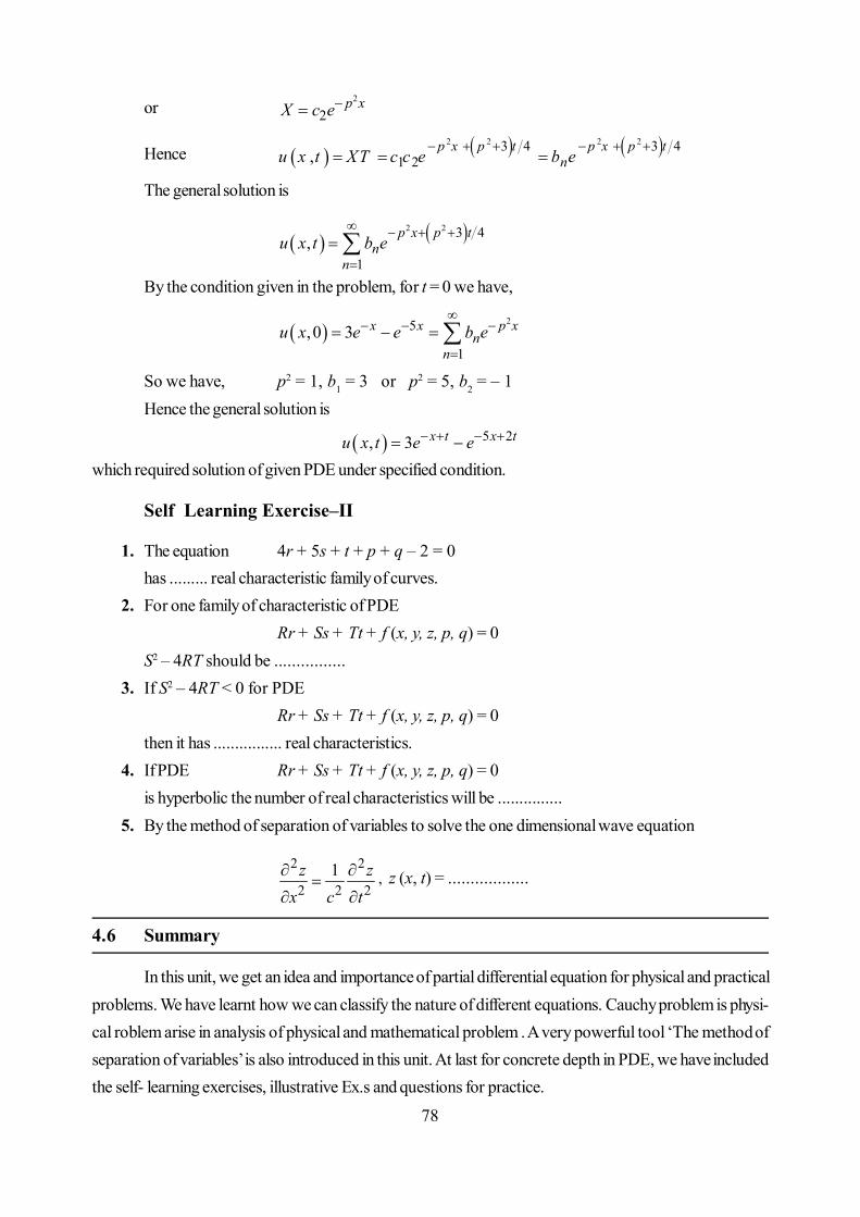
78
or2
2p xX c e
Hence 2 2 2 23 4 3 41 2,
p x p t p x p tnu x t XT c c e b e
The general solution is
2 2 3 4
1,
p x p t
nn
u x t b e
By the condition given in the problem, for t = 0 we have,
25
1,0 3 x x p x
nn
u x e e b e
So we have, p2 = 1, b1 = 3 or p2 = 5, b2 = – 1Hence the general solution is
5 2, 3 x t x tu x t e e
which required solution of given PDE under specified condition.
Self Learning Exercise–II
1. The equation 4r + 5s + t + p + q – 2 = 0has ......... real characteristic family of curves.
2. For one family of characteristic of PDERr + Ss + Tt + f (x, y, z, p, q) = 0
S2 – 4RT should be ................3. If S2 – 4RT < 0 for PDE
Rr + Ss + Tt + f (x, y, z, p, q) = 0then it has ................ real characteristics.
4. If PDE Rr + Ss + Tt + f (x, y, z, p, q) = 0is hyperbolic the number of real characteristics will be ...............
5. By the method of separation of variables to solve the one dimensional wave equation
2 2
2 2 21z z
x c t
, z (x, t) = ..................
4.6 Summary
In this unit, we get an idea and importance of partial differential equation for physical and practicalproblems. We have learnt how we can classify the nature of different equations. Cauchy problem is physi-cal roblem arise in analysis of physical and mathematical problem . A very powerful tool ‘The method ofseparation of variables’ is also introduced in this unit. At last for concrete depth in PDE, we have includedthe self- learning exercises, illustrative Ex.s and questions for practice.

79
4.7 Answers to Self-Learning Exercises
Exercise – I1. (i) b (ii) c (iii) a (iv) a2. See § 4 3. xy log y < 04. Parabolic 5. Hyperbolic6. Elliptic if t2 – 4x < 0,Hyperbolic if t2 – 4x > 0 and Parabolic if t2 – 4x = 0
Exercise – II1. 2 2. S2 – 4RT = 0 3. Zero
4. 2 5. X (x) T (t)
4.8 Exercise
1. Find the characteristics of
(i) 4r + 5s + t + p + q – 2 = 0 [Ans. 1 2, and xy x c y cy
]
(ii) (sin2 x)r + (2cos x)s – t = 0 [Ans. y + cosec x – cot x = c1 ; y + cosec x + cot x = c2]2. Show that the equation uxx + xuyy + uy = 0 is elliptic for x > 0 and hyperbolic for x < 0.3. Find whther the following PDE are parabolic or elliptic
(i) 2 2
22 2 0u ux u
t x
[Ans. Hyperbolic if x > 0, parabolic if x = 0 and elliptic if x < 0 ]
(ii)2 2 2
2 22 0u u u utx t xt x
[Ans. tx < 1 for hyperbolic, tx > 1 for elliptic and tx = 1 for parabolic]4. Solve by the method of separation of variables :
34 ; 0, 8 yu u u y ex y
[Ans. u (x, y) = 8e–3y-12x]
5. Solve by the method of separation of variables :
42 ; ,0 10 6x xu u u u x e et x
[Ans. u (x, t) = 10e–(x+3t) – 6e–2(2x+3t)]
6. Solve 2uxx – uy = 0 by separation of variables. [Ans. 2,kx kx kyu x y Ae Be e
]
7. Solve the following PDE by the method of separation of variables,(i) 4ux + uy = 3u and u (0, y) = e–5y [Ans. u (x, y) = e2x – 5y]
(ii)2
2 2u utx
; u (x, 0) = x (a – x) [Ans. u (x, y) = x (a – x) 2 2 p te ]
(iii) y3ux + x2uy = 0 [Ans. 3 43 4,
k x yu x y ce
]

80
8. Use the method of separation of variables to solve the equation,
2
2 2u u uyx
[Ans. 2 2, cos sin p yu x y A px B px e ]
9. Solve the method of separation of variables,
3 2 0 ; ,0 4 xu u u x ex y
[Ans. 3 2, 4 x yu x y e ]
10. Solve by method of separation of variables,
54 3 ; 0, 4 y yu u u u y e ex y
[Ans. 2 5, 4 x y x yu x y e e ]
11. Solve by method of separation of variables,
2u u ux t
= 0 when u (x, 0) = 6e–3x [Ans. 3 2, 6 x tu x y e ]

81
Unit 5 : Laplace, Wave and Diffusion Equations AndCanonical Forms
Structure of the Unit
5.0 Objective
5.1 Introduction
5.2 Laplace, Wave and Diffusion Equations
5.2.1 Laplace Equations
5.2.2 Wave Equations
5.2.3 Diffusion Equations
5.3 Canonical Forms
5.4 Summary
5.5 Answers to Self-Learning Exercises
5.6 Exercise
5.0 Objective
After studying this unit, you should be able to know application of partial differential equations. You
will get an idea of wave, diffusion and Laplace equations in different coordinate system and their solutions.
You will also study the reduction of the second order P.D.E’s to canonical forms.
5.1 Introduction
In physical and engineering application, PDE’s of second order are of utmost significance. These
equations arise in the modelling of vibration of string and membranes, theory of hydraulics, gravitational
and potential problems and so on. Since a comprehensive treatment of the subject is not possible in this
unit, we restrict our study to a consideration of some special types of equations.
5.2 Laplace, Wave and Diffusion Equations
In applied mathematics and theoretical physics three types of equations occur frequently. These
are
(i) Laplace Equation
(ii) Wave Equation and
(iii)Diffusion Equation.
In many practical problems the solution of these equations may be obtained with the help of sepa-
ration of variables.

82
5.2.1 Laplace Equation
One of the most important PDE appearing in theoretical physics is Laplace’s equation. It isusually written as
2u = 0 .....(1)where the operator 2, known as Laplacian depends on the coordinate system chosen. It is an ellipticPDE.
(i) in three dimensions, this equation in Cartesian system of coordinates (x, y, z) is written as
2 2 2
2 2 2 0u u ux y z
.....(2)
(ii) in cylindrical polar coordinates (r, , z), eq. (2) becomes
2 2 2
2 2 2 21 1 0
u u u ur rr r z
.....(3)
(iii) in antisymmetric case i.e. u is independent of , therefore equation (3) reduces to
2 2
2 21 0
u u ur rr z
.....(4)
(iv) in spherical polar coordinates (r, , ), eq. (2) reduces to
2 2 2
2 2 2 2 2 2 22 1 cot 1 0
sin
u u u u ur rr r r r .....(5)
(v) when u is independent of the azimuthal angle , (5) reduces to
2 2
2 2 2 22 1 cot 0
u u u ur rr r r
or 2 1 sin 0sin
u ur
r r .....(6)
(vi) in two dimensions, Laplace equation is
2 2
2 2 0u ux y
.....(7)
in Cartesian coordinates (x, y) and
2 2
2 2 21 1 0
u u ur rr r
.....(8)
in polar coordinates (r, ).
Equation (7) is also known as Harmonic equation.
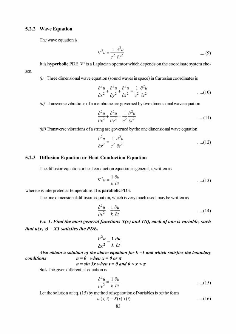
83
5.2.2 Wave Equation
The wave equation is2
22 2
1
uu
c t.....(9)
It is hyperbolic PDE. is a Laplacian operator which depends on the coordinate system cho-sen.
(i) Three dimensional wave equation (sound waves in space) in Cartesian coordinates is2 2 2 2
2 2 2 2 21u u u u
x y z c t
.....(10)
(ii) Transverse vibrations of a membrane are governed by two dimensional wave equation2 2 2
2 2 2 21
u u ux y c t .....(11)
(iii)Transverse vibrations of a string are governed by the one dimensional wave equation2 2
2 2 21u u
x c t
.....(12)
5.2.3 Diffusion Equation or Heat Conduction Equation
The diffusion equation or heat conduction equation in general, is written as
2 1 uuk t
.....(13)
where u is interpreted as temperature. It is parabolic PDE.The one dimensional diffusion equation, which is very much used, may be written as
2
21
u uk tx
.....(14)
Ex. 1. Find the most general functions X(x) and T(t), each of one is variable, suchthat u(x, y) = XT satisfies the PDE.
u uk tx
2
21=
Also obtain a solution of the above equation for k =1 and which satisfies the boundaryconditions u = 0 when x = 0 or
u = sin 3x when t = 0 and 0 < x < Sol. The given differential equation is
2
21u u=k tx
.....(15)
Let the solution of eq. (15) by method of separation of variables is of the formu (x, t) = X(x) T(t) .....(16)
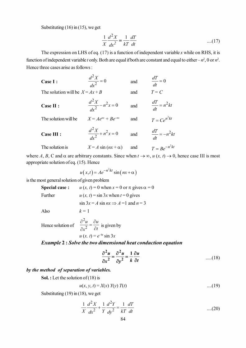
84
Substituting (16) in (15), we get21 1
2d X dT
X kT dtdx....(17)
The expression on LHS of eq. (17) is a function of independent variable x while on RHS, it isfunction of independent variable t only. Both are equal if both are constant and equal to either – n2, 0 or n2.Hence three cases arise as follows :
Case I :2
2 0d Xdx
and 0dTdt
The solution will be X = Ax + B and T = C
Case II :2
22 0
d X n xdx
and 2dT n ktdt
The solution will be X = Aenx + Be–nx and 2 n ktT Ce
Case III :2
22 0
d X n xdx
and 2dT n ktdt
The solution is X = A sin (nx + ) and 2 n ktT Bewhere A, B, C and are arbitrary constants. Since when t , u (x, t) 0, hence case III is mostappropriate solution of eq. (15). Hence
2
, sinn ktu x t Ae nx
is the most general solution of given problemSpecial case : u (x, t) = 0 when x = 0 or gives = 0Further u (x, t) = sin 3x when t = 0 gives
sin 3x = A sin nx A =1 and n = 3Also k = 1
Hence solution of2
2
u utx
is given by
u (x. t) = e–9t sin 3xExample 2 : Solve the two dimensional heat conduction equation
u u uk tx y
2 2
2 21
.....(18)
by the method of separation of variables.Sol. : Let the solution of (18) is
u(x, y, t) = X(x) Y(y) T(t) ....(19)Substituting (19) in (18), we get
2 2
2 21 1 1
d X d Y dT
X Y kT dtdx dy....(20)
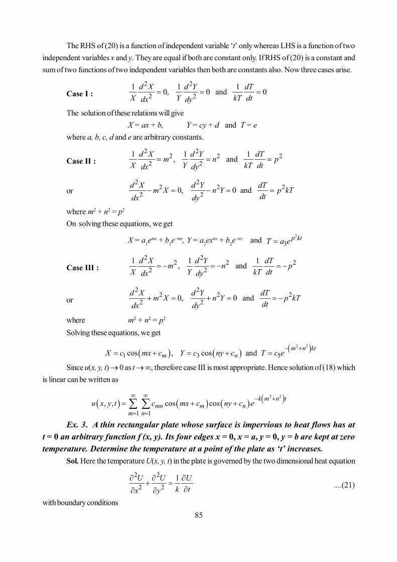
85
The RHS of (20) is a function of independent variable ‘t’ only whereas LHS is a function of twoindependent variables x and y. They are equal if both are constant only. If RHS of (20) is a constant andsum of two functions of two independent variables then both are constants also. Now three cases arise.
Case I :2 2
2 21 1 10, 0 and 0
d X d Y dTX Y kT dtdx dy
The solution of these relations will giveX = ax + b, Y = cy + d and T = e
where a, b, c, d and e are arbitrary constants.
Case II :2 2
2 2 22 2
1 1 1, and d X d Y dTm n p
X Y kT dtdx dy
or2 2
2 2 22 20, 0 and
d X d Y dTm X n Y p kTdtdx dy
where m2 + n2 = p2
On solving these equations, we get
X = a1emx + b1e
–mx, Y = a2exnx + b2e–nx and
2
3p ktT a e
Case III :2 2
2 2 22 2
1 1 1, and d X d Y dTm n p
X Y kT dtdx dy
or2 2
2 2 22 20, 0 and
d X d Y dTm X n Y p kTdtdx dy
where m2 + n2 = p2
Solving these equations, we get
2 2
1 3 5cos , cos and
m n kt
m nX c mx c Y c ny c T c e
Since u(x, y, t) 0 as t , therefore case III is most appropriate. Hence solution of (18) whichis linear can be written as
2 2
1 1, , cos cos
k m n t
mn m nm n
u x y t c mx c ny c e
Ex. 3. A thin rectangular plate whose surface is impervious to heat flows has att = 0 an arbitrary function f (x, y). Its four edges x = 0, x = a, y = 0, y = b are kept at zerotemperature. Determine the temperature at a point of the plate as ‘t’ increases.
Sol. Here the temperature U(x, y, t) in the plate is governed by the two dimensional heat equation
2 2
2 21
U U Uk tx y
....(21)
with boundary conditions

86
0, , 0, , , 0, ,0, 0, , , 0 U y t U a y t U x t U x b t .....(22)
and initial condition isU (x, y, t) = f (x, y) .....(23)
Proceeding similarily to Ex.2, we find that if solution of (21) may be assumed asU (x, y, 0) = X(x) Y(y)T(t)
then X = c1 cos (mx + cm) = A1cos mx+ B1sin mx,Y = A2 cos nx + B2 sin nx
and 2 2
3
k m n tT A e
Using boundary conditions (22), we find thatA1 = 0, B1 sin ma = 0, A2 = 0, B2 sin nb = 0
A1 = 0 = A2, sin ma = sin u and sin nb = sin v (u, = 1, 2, 3 ....) asB1 0 and B2 0
Thus A1 = 0 = A2, uma
and
vnb
Hence the general solution of (21) will be
2 22
2 2
1 1, , sin sin
uk ta b
uvu
u x yU x y t F ea b
Now under initial condition (23), we have
1 1
, , , sin sin
uu
u x yU x y o f x y Fa b .....(24)
which is a double Fourier series of f (x, y).
Hence 0 0
4 , sin sin
a b
uvx y
u x v yF f x y dxdyab a b .....(25)
Thus (24) is a general solution of (21) under boundary and initial condition (22) and (23) whereconstant Fuv as given by (25).
Ex. 4. By separating the variables, show that the one dimensional wave equation
u ux c t
2 2
2 2 21
.....(26)
has solution of the form A in x inctexp where A and n are constants.
Sol. Let the solution of (26) isu(x, t) = X(x) T(t) ....(27)
Substituting (27) in (26), we get
2 2
22 2 2
1 1 say d X d T n
X dx c T dt

87
2 2
2 2 22 20 and 0
d X d Tn X n c Tdx dt
Solving these we get
1 2andin x in ctX c e T c e .....(28)
Hence from (27) and (28), we get the solution of (26) asu(x, t) = A exp ( in x in ct)
Ex. 5. A tightly stretched sting which has fixed end points x = 0 and x = l is initiallyin a position given by y = k sin3 (x/l). It is released from rest from this position. Find thedisplacement y (x, t).
Sol. Since the string is tightly stretched initially between two fixed points and released from rest, itwill make transverse vibrations in (x, y) plane. The displacement y(x, t) of any point on it will be a gov-erned by the following wave equation
2 2
2 2 21y y
x c t
.....(29)
with the boundary conditionst > 0 : y(0,t) = 0 = y(l, t) .....(30)
and the initial conditiont = 0 : y(x,0) = k sin3(x/l) .....(31)
which also implies0
0t
yt
Applying the method of separation of variables if solution of (29) is of the form X(x)T(t) wefind that
X = A cos x + B sin xand T = C cos ct + D sin ct ....(32)Using boundary condition (30), we get
A = 0 and sin 0 0 1, 2,3....nB B n
Hence Xn(x) = An sin (n/l) ....(33)
Under initial condition 0
0t
yt
, we get D = 0 from (32). Therefore
Tn(t) = Bn cos (nct/l) ....(34)Hence (33) and (34), we get the general solution of (29) as
, sin cos ,
n nn x n cty x t C n N
where Cn = An Bn is an arbitrary constant
Hence 1 1
, , sin cos
n n
n n
n x n cty x t y x t C .....(35)
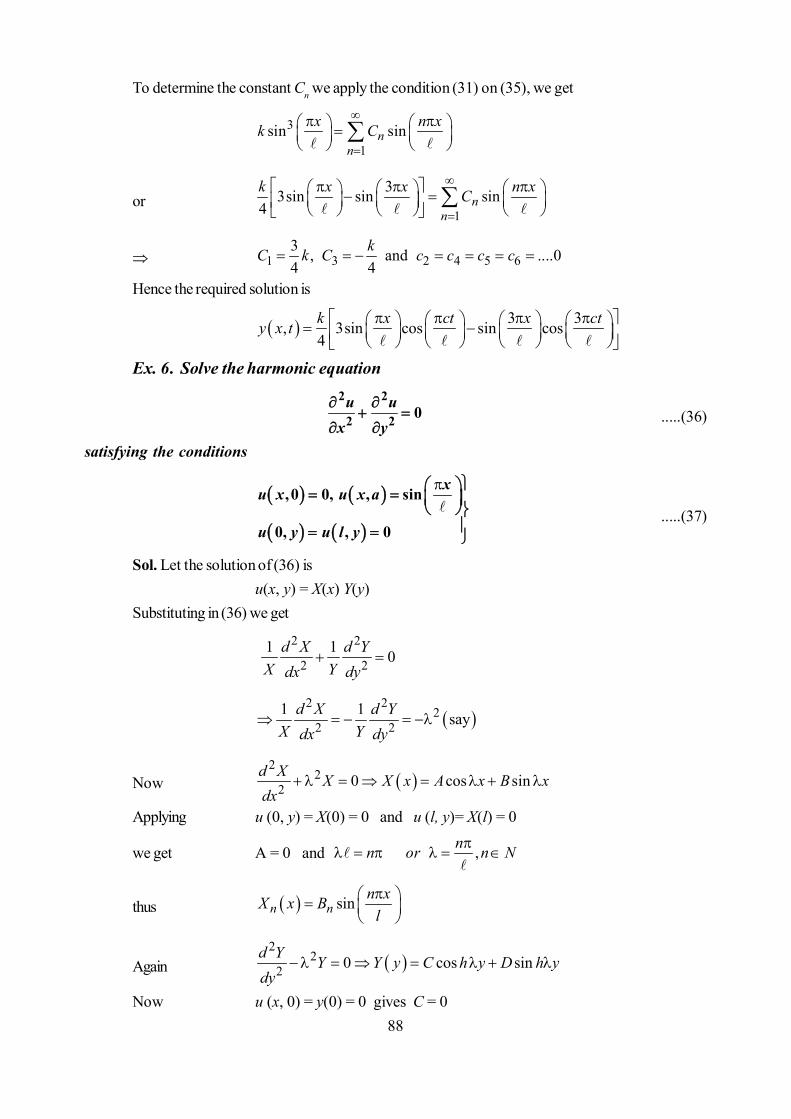
88
To determine the constant Cn we apply the condition (31) on (35), we get
3
1sin sin
nn
x n xk C
or1
33sin sin sin4
n
n
k x x n xC
1 3 2 4 5 63 , and ....04 4
kC k C c c c c
Hence the required solution is
3 3, 3sin cos sin cos4
k x ct x cty x t
Ex. 6. Solve the harmonic equation
u ux y
2 2
2 2 0
.....(36)
satisfying the conditions
xu x u x a
u y u l y
,0 0, , sin
0, , 0
.....(37)
Sol. Let the solution of (36) isu(x, y) = X(x) Y(y)
Substituting in (36) we get
2 2
2 21 1 0
d X d YX Ydx dy
2 2
22 2
1 1 say d X d Y
X Ydx dy
Now 2
22 0 cos sin
d X X X x A x B xdx
Applying u (0, y) = X(0) = 0 and u (l, y)= X(l) = 0
we get A = 0 and ,
nn or n N
thus sin
n nn xX x B
l
Again 2
22 0 cos sin
d Y Y Y y C h y D h ydy
Now u (x, 0) = y(0) = 0 gives C = 0

89
thus sin
n nn yY y D
l
Hence we have , sin sin
n n n nn x n yu x y X x Y y F h
l lwhere Fn is arbitrary constant. Therefore
1
, sin sin
nn
n x n yu x y F hl l
Now applying the boundary conditionu (x, a) = sin (x/l)
We find that1
sin sin sin
nn
x n x n aF h xl l l
Equating coefficients of like terms, we getF1 sinh (a/l) = 1 and F2 = F3 = .... = 0
Hence, the required solution is
, cosec sin sin
a x yu x y h hl l l
5.3 Canonical Forms
Let us consider the equations of the typeRr + Ss + Tt + f (x, y, z, p, q) = 0 ....(1)
where R, S, T are continuous functions of x and y possessing continuous partial derivatives of as high asorder as necessary. It is a typical class of semi-linear equations of the type of
Rr + Ss + Tt = VChanging the independent variables x, y to , such that
= (x, y), = (x, y) .....(2)z = z () ....(3)
Here it is assumed that are doubly differentiable and the transformation from (x, y)–planeto ( )–plane is locally one to one. This requires that the Jacobian of the transformation isnonzero, i.e.
,0
,
Jx y x y y x
Now from (2) and (3), we get
z z zp zx x x x x
z z zq zy y y y y

90
2
2
z z zrx x x xx
2 22 2 2 2 2
2 2 2 22 2 2
z z z z zx x x x x x
2 2
2
z z z zsx y x x y y x y
2 2 2 2
2z z z z
x y x y x y x y x y
and22 2
2 2
z z z zty y y y yy
22 2 2 2
2 2 22
z z z zy y y y y .....(4)
Now substituting these values in (1), it takes the form
2 2 2
2 22 , , , , 0
z z z z zA B C F z .....(5)
where22
A R S Tx x y y .....(6)
12
B R S Tx x x y x y y y
.....(7)
22 C R S T
x x y y .....(8)
and , , , ,
z zF z
is obtained from the transformed form of f (x, y, z, p, q) and the remaining terms containing first orderpartial derivatives of transformed Rr, Ss, and Tt.
One of the relations satisfied by A, B, C and R, S, T which can be easily seen, is
2 2 21 44
AC B RT S J .....(9)
We shall now determine the functional relationship [equations (2)] of with x and y so that thetransformed equation (5) takes the simplest possible form.
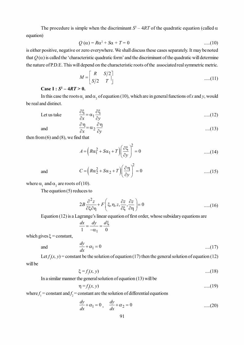
91
The procedure is simple when the discriminant S2 – 4RT of the quadratic equation (called equation)
Q () = R2 + S + T = 0 .....(10)is either positive, negative or zero everywhere. We shall discuss these cases separately. It may be notedthat Q () is called the ‘characteristic quadratic form’ and the discriminant of the quadratic will determinethe nature of P.D.E. This will depend on the characteristic roots of the associated real symmetric metric.
22
R SM
S T .....(11)
Case I : S2 – 4RT > 0.In this case the roots and of equation (10), which are in general functions of x and y, would
be real and distinct.
Let us take 1x y
.....(12)
and 2x y ....(13)
then from (6) and (8), we find that
2
21 1 0A R S T
y
.....(14)
and 2
22 2 0C R S T
y
.....(15)
where and are roots of (10).The equation (5) reduces to
22 , , , , 0
z z zB F z .....(16)
Equation (12) is a Lagrange’s linear equation of first order, whose subsidary equations are
11 0dx dy d
which gives = constant,
and 1 0dydx
....(17)
Let f1(x, y) = constant be the solution of equation (17) then the general solution of equation (12)will be
= f1(x, y) ....(18)In a similar manner the general solution of equation (13) will be
= f2(x, y) .....(19)where f1 = constant and f2 = constant are the solution of differential equations
1 0dydx
, 2 0dydx
.....(20)

92
respectively. Relations (18) and (19) are the desired transformations for independent variables whichreduce the given equations (1) to the form (16).
Now from (9), we have
2
2 21 44
AC B RT Sx y y x
.....(21)
This shows that the sign of (AC – B2) is the same as of (4RT – S2) i.e. it is invariant undertransformation.
Therefore, when A = C = 0, from (21), we have
2
2 24 4B S RTx y y x
.....(22)
Since we have assumed that S2 > 4RT, it implies from (22) that B2 > 0 i.e. B 0 and therefore wemay devide both sides of equation (16) by it and write it finally as
21 , , , ,
z z zz .....(23)
which is the canonical form of equation (1) when S2 – 4RT > 0.
Case II : S2 – 4RT = 0.
In this case the two roots of the quadratic equation (10) are equal i.e. = Therefore one of the
functions, say will be defined by equation (18) of case I. We may now take to be any suitable function
of x and y which should be independent of . Therefore, as before, A = 0 but C 0. Further, from (21),
since S2 – 4RT = 0 we have
B = 0
Hence equation (5) reduces to
2
2 , , , , 0
z z zC F z
or2
22 , , , ,
z z zz .....(24)
which is the canonical form of the equation (1) when S2 – 4RT = 0.Case III : S2 – 4RT < 0.This is particularly the same as case I except that the roots of the quadratic equation (10) in this
case are complex. If we proceed in the same manner as we did in case I, we shall arrive at equation (21)but in this case the variables are not real and in fact complex conjugates. To get a real cononical form wetransform the independent varialdes and again be the following relations.
1 1,2 2
i ....(25)
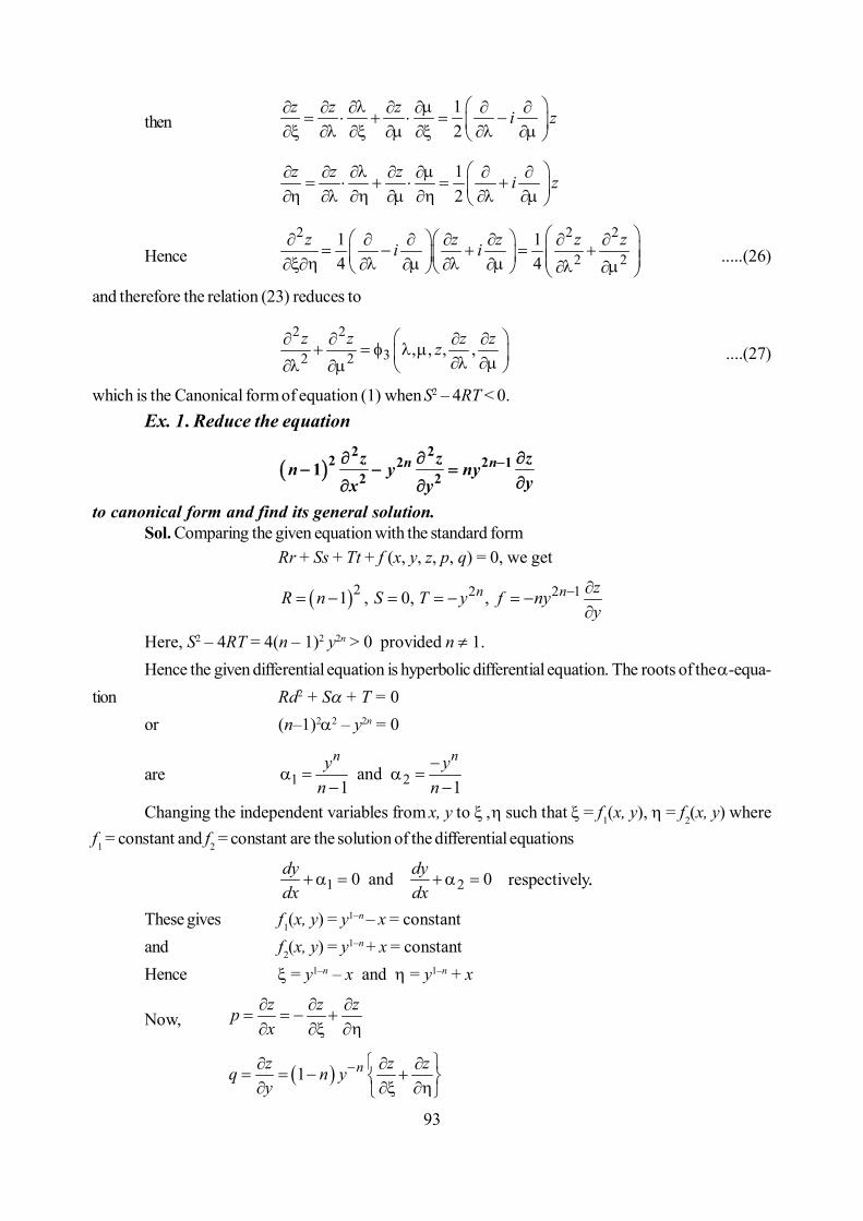
93
then12
z z z i z
12
z z z i z
Hence2 2 2
2 21 14 4
z z z z zi i .....(26)
and therefore the relation (23) reduces to
2 232 2 , , , ,z z z zz
....(27)
which is the Canonical form of equation (1) when S2 – 4RT < 0.Ex. 1. Reduce the equation
2 2
2 2 2 12 21 n nz z z
n y nyyx y
to canonical form and find its general solution.
Sol. Comparing the given equation with the standard formRr + Ss + Tt + f (x, y, z, p, q) = 0, we get
2 2 2 11 , 0, ,n n zR n S T y f nyy
Here, S2 – 4RT = 4(n – 1)2 y2n > 0 provided n 1.Hence the given differential equation is hyperbolic differential equation. The roots of the -equa-
tion Rd2 + S + T = 0or (n–1)22 – y2n = 0
are 1 2and1 1
n ny yn n
Changing the independent variables from x, y to such that = f1(x, y), = f2(x, y) where
f1 = constant and f2 = constant are the solution of the differential equations
1 20 and 0 dy dydx dx
respectively..
These gives f1(x, y) = y1–n – x = constantand f2(x, y) = y1–n + x = constantHence = y1–n – x and = y1–n + x
Now,z z zpx
1 nz z zq n yy

94
2 2 2 2
2 2 22
z z z zrx
2 2 2 22 2
2 2 21 2
nz z z zt n yy 11
n z zn n y
Therefore, the given equation reduces to
2 2 2 2 2 22 2
2 2 2 21 2 1 2z z z z z zn n
1 11 1n nz z z zn n y n n y
or 224 1 0zn
or2
0z
which is the required canonical form if n 1.The general solution of the above equation may be easily obtained as
1 1z where and arbitrary functions of and respectively. Changing to original variables we get finally
1 11 2
n nz y x y x
Note : If n = 1, the character of the given differential equation changes. It becomes a parabolicequation, viz.
2
2 0z zyyy
whose general solution is
1 2logz x y x .
Ex.2. Reduce the equation
z z zx yx y
2 2 2
2 22 0
to canonical form and hence solve it.Sol. Comparing the given equation with the standard form Rr + Ss + Tt + f (x, y, z, p, q) = 0,we get, R = 1, S = 2, T = 1, f = 0Here S2 – 4RT = 4 – 4 = 0Hence the given equation is a parabolic differential equation.The roots of the -equation
R2 + S + T = 0
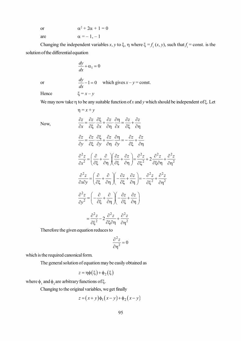
95
or 2 + 2 + 1 = 0
are = – 1, – 1
Changing the independent variables x, y to , where = f1 (x, y), such that fi = const. is the
solution of the differential equation
1 0dydx
or 1 0dydx
which gives x – y = const.
Hence = x – y
We may now take to be any suitable function of x and y which should be independent of . Let
= x + y
Now,z z z z zx x x
z z z z zy y y
2 2 2 2
2 2 22z z z z z zx
2 2 2
2 2z z z z z
x y
2
2z z z
y
2 2 2
2 22z z z
Therefore the given equation reduces to2
2 0z
which is the required canonical form.The general solution of equation may be easily obtained as
2z
where 1 and 2 are arbitrary functions of .Changing to the original variables, we get finally
1 2z x y x y x y
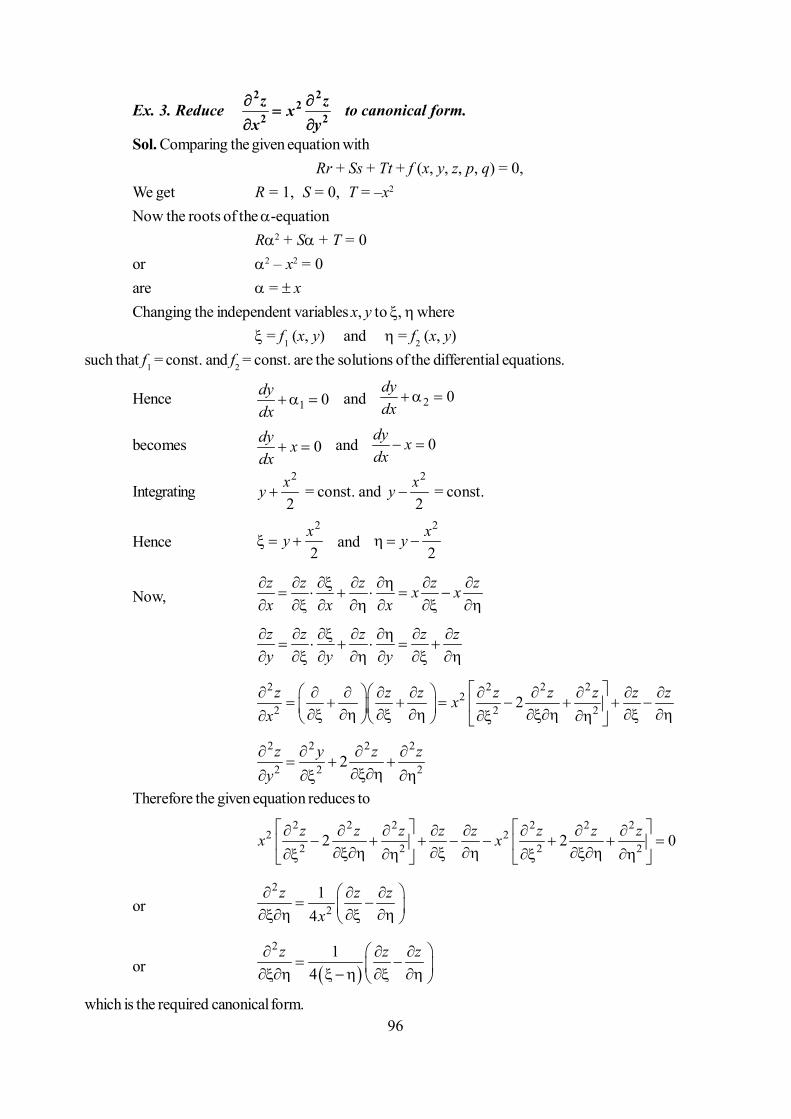
96
Ex. 3. Reduce 2 2
22 2z zx
x y
to canonical form.
Sol. Comparing the given equation withRr + Ss + Tt + f (x, y, z, p, q) = 0,
We get R = 1, S = 0, T = –x2
Now the roots of the -equationR2 + S + T = 0
or 2 – x2 = 0are = xChanging the independent variables x, y to , where
= f1 (x, y) and = f2 (x, y)such that f1 = const. and f2 = const. are the solutions of the differential equations.
Hence 1 0 dydx
and 2 0 dydx
becomes 0dy xdx
and 0dy xdx
Integrating2
2xy = const. and
2
2xy = const.
Hence2
2xy and
2
2xy
Now,z z z z zx xx x x
z z z z zy y y
2 2 2 22
2 2 22
z z z z z z z zxx
2 2 2 2
2 2 22z y z zy
Therefore the given equation reduces to2 2 2 2 2 2
2 22 2 2 22 2 0
z z z z z z z zx x
or2
21
4z z z
x
or 2 1
4z z z
which is the required canonical form.
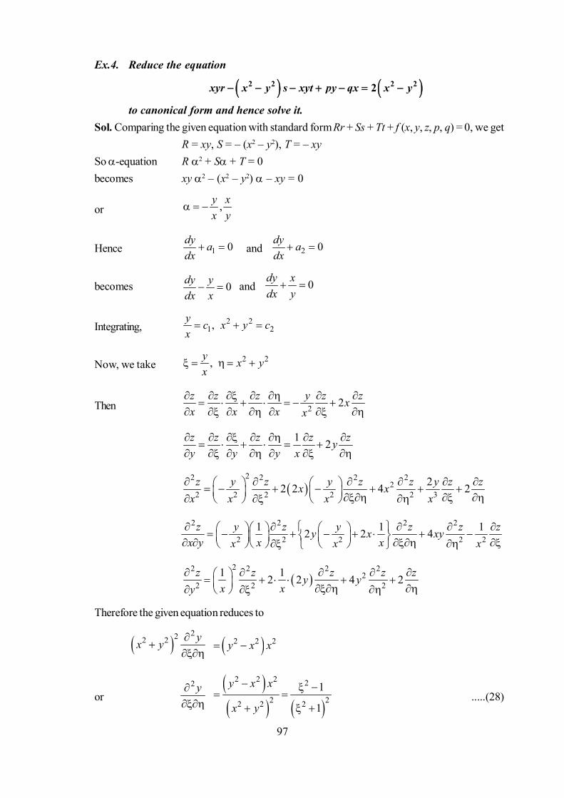
97
Ex.4. Reduce the equation
2 2 2 22xyr x y s xyt py qx x y
to canonical form and hence solve it.Sol. Comparing the given equation with standard form Rr + Ss + Tt + f (x, y, z, p, q) = 0, we get
R = xy, S = – (x2 – y2), T = – xySo -equation R 2 + S + T = 0becomes xy 2 – (x2 – y2) – xy = 0
or , y xx y
Hence 1 0 dy adx and 2 0
dy adx
becomes 0dy ydx x
and 0 dy xdx y
Integrating, 2 21 2,
y c x y cx
Now, we take 2 2,y x yx
Then 2 2
z z z y z zxx x x x
1 2z z z z zyy y y x
22 2 2 2
22 2 2 2 2 3
22 2 4 2 z y z y z z y z zx x
x x x x
2 2 2 2
2 2 2 2 21 1 12 2 4z y z y z z zy x xy
x y x xx x x
22 2 2 2
22 2 2
1 12 2 4 2 z z z z zy y
x xy
Therefore the given equation reduces to
222 2
yx y 2 2 2y x x
or2 y
2 2 2 2
2 22 2 2
1
1
y x x
x y
.....(28)

98
Integrating (28) w.r.t. , we get
z
2
22
1
1d
2 22
21 1
d d
2 2212
2 1 11 12 1 1 1d d
z 2 1
Integrating it, we get
z = 1 22 1
or z = 2 21 2
yxy x yx
Self Learning Exercise1. The Harmonic equation is ....
2.2 2
2 21u u uk tx y
is two-dimensional ........... equation.
3. Write general Laplace’s equation.
4. Write wave equation.
5. Give a common method for solving Laplace, wave and diffusion equations.
5.4 Summary
In this unit, we have covered nature and types of Laplace, wave and diffusion equations and their
solutions under different boundary and initial conditions, with illustrative examples. We have also presented
the canonical form of PDE and its general solution also for hyperbolic, parabolic and elliptic equations.
5.5 Answers of Self-Learning Exercises
1.2 2
2 2 0u ux y
2. Diffusion
3. 2 0u 4.2 2
2 2 21u u
x c t
5. Separation of variables

99
5.6 Exercise
1. A string is stretched between the fixed point O (x = 0) and A (x = 1) and released at rest from theposition U(x, 0) = A sin x. Find the formula for its subsequent displacement U(x ,t)
[Ans : U (x, t) = A cos ct cos x]2. A string is stretched between the fixed points (0, 0) and (l, 0). If it is released at rest from the initial
deflection
2 ; 02
2 ;2
k lx xlf xk ll x x ll
where ‘k’ is arbitrary constant. Find the expression of deflection of the string at any instant ‘t’.
[Ans : 28 sin cos 1 3 3, sin cos ....
9
k x ct x ctU x tl l l l
3. A tightly string stretched string with fixed end points x = 0 and x = is initially at rest in itsequilibrium position. If it is set vibrating by giving to each of its points an initial velocity
00.03sin 0.04sin 3
t
U x xt
then find the displacement U (x, t) at any point x and at any instant t.
[Ans. 1, 0.03sin sin 0.01333sin 3 sin 3U x t x ct x ctc
]
4. Solve ytt = 4yxx, y (5, t) = 0 = y (5, t), y (x, 0) = 0 and 0
5sint
y f x xt
[Ans. 5, sin sin 22
y x t x t
]
5. Solve diffusion equation 2
2
u ut x
, 0 < x < l, t > 0
u(x, 0) = 3 sin n x, u (0, t) = 0, u(l, t) = 0.
[Ans. 2 2
1, 3 sin
n t
nu x t e n x ]
6. The temperature distribution in a bar of length which is perfectly insulated at ends x = 0 and x =is governed by PDE
2
2
u ut x
Assuming the initial temperature distribution as u(x, 0) = cos 2x. Find the temperature distribution
at any instant of time. [Ans. u(x, t) = e–4t cos2x]
7. A homogeneous rod of conducting material of length 100 cm has its ends kept at zero temperature
and the temperature initially is
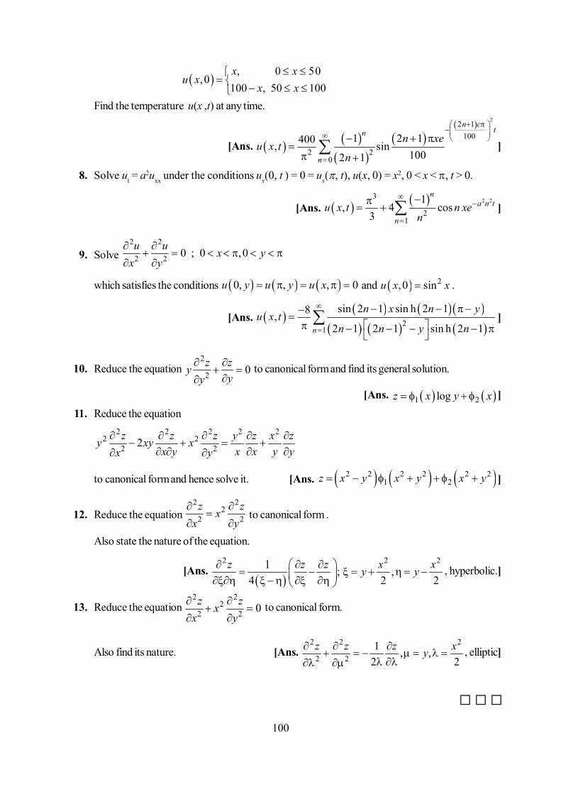
100
, 0 50,0
100 , 50 100
x xu x
x xFind the temperature u(x ,t) at any time.
[Ans.
22 1
100
2 20
1 2 1400, sin1002 1
n ctn
n
n xeu x t
n]
8. Solve ut = a2uxx under the conditions ux(0, t ) = 0 = ux(, t), u(x, 0) = x2, 0 < x < , t > 0.
[Ans. 2 23
21
1, 4 cos
3
na n t
nu x t n xe
n]
9. Solve 2 2
2 2 0 ; 0 ,0
u u x y
x y
which satisfies the conditions 0, , , 0 u y u y u x and 2,0 sinu x x .
[Ans. 2
1
sin 2 1 sin h 2 18,2 1 2 1 sin h 2 1
n
n x n yu x t
n n y n]
10. Reduce the equation 2
2 0z zyyy
to canonical form and find its general solution.
[Ans. 1 2logz x y x ]
11. Reduce the equation2 2 2 2 2
2 22 22z z z y z x zy xy x
x y x x y yx y
to canonical form and hence solve it. [Ans. 2 2 2 2 2 21 2z x y x y x y ]
12. Reduce the equation 2 2
22 2z zx
x y
to canonical form .
Also state the nature of the equation.
[Ans.
2 2 21 ; ,4 2 2
z z z x xy y , hyperbolic.]
13. Reduce the equation 2 2
22 2 0
z zx
x y to canonical form.
Also find its nature. [Ans. 2 2 2
2 21 , ,
2 2
z z z xy , elliptic]

101
Unit 6 : Eigenvalues, Eigenfunctions and Sturm-LiouvilleBoundary Value Probleon
Structure of the Unit
6.0 Objective
6.1 Introduction
6.2 Linear Homogeneous Boundary Value Problem
6.3 Eigenvalues and Eigenfunctions
6.3.1 Eigenvalue
6.3.2 Eigenfunction
6.4 Sturm-Liouville Problem
6.5 Orbnogonality of Eigenfunctions
6.6 Important Theorems for Sturm-Liouville System
6.6.1 Theorem 1
6.6.2 Theorem 2
6.6.3 Theorem 3
6.6.4 Theorem 4
6.7 Summary
6.8 Answer to Self-Learning Exercise
6.9 Exercise
6.0 Objective
After completing the present unit, you will get a basic knowledge about eigenvalue andeigenfunction of boundary value problems. You will study special boundary value problem known as Sturm-Liouvelle problem and properties of eigenfunctions in later part of unit. The knowledge which you gainhere, can be used to study various special functions that arise in physical and engineering problems.
6.1 Introduction
In the eighteenth century much attention was given to the problem of determing the mathematicallaws governing the notion of a vibrating string with fixed end points. We wish to motivate the physics ofvibrating string. In the last unit, we dealt the wave equation in detail with some other physical problemswhere we had derived boundary value problems for seeking non-trivial solution of partial differental equa-

102
tions involved in formulating physical problems. In this unit we study the condition of parameter involvedin boundary value problem and corresponding non-trivial solution. We will also see special boundaryvalue problem, known as Sturm-Liouville problem in detail which helps in studying regular boundaryvalue problem and special functions in future.
6.2 Linear Homogeneous Boundary Value Problems
In previous unit, we have noticed that most important application of the idea is in boundary valueproblems of any type. For second order linear differential equation, boundary value problem is definedas
Ly = h .....(1)where L is a second order linear differential operator defined on a finite interval [a, b] and h is a functionin [a, b] and pair of homogeneous boundary conditions of the form
1 y (a) + 2 y (b) + 3 y(a) + 4 y(b) = 1 .....(2)1 y (a) + 2 y (b) + 3 y (a) + 4 y (b) = 2 .....(3)
where i, i and i for i = 1, 2 are constants. The problem (1) with boundary conditions (2) and (3) isknown as linear homogeneous boundary value problem. In this problem, we seek all non-trivial func-tions of y(x) in [a, b] which simultaneously satisfy differential equation (1) and boundary conditions (2)to (3).
For example, y + y = 0 .....(4)with boundary conditions
y(0) = 0 and y() = 0 .....(5)is a boundary value problem of above type on the interval [a, b]. The parameter ‘’ in (4) is free toassume any real value.
The situation with boundary conditions is quite different from that for initial condition. The initialvalue problem is a sophisticated variation of the fundamental theorem of calcalus. The boundary valueproblem is rather more subtle.
6.3 Eigenvalues and Eigenfunctions
In previous study, we have considered initial value problem, in which the solution of second or-der differential equation is sought that satisfies two conditions at a single value of the independent vari-able. Here we have absolutely different situation for we wish to satsfy one condition at each of twodistinct values of independent variable x. The part of our task is to discover the values of s for whichproblem can be solved for getting non-trivial solution. The solution of given problem in (4) with bound-ary conditions (5) is not difficult to find. We simply apply the boundary conditions to the general solu-tion. But we have to analyse the solution for all possible values of s. So, three cases arise as follows.
Case I : is negative or < 0Let = –m2
The given problem (4) with (5) becomesy – m2y = 0 .....(1)

103
and y(0) = 0 and y() = 0so, the general solution is
y(x) = c1emx + c2e
–mx
Now y(0) = 0 c1 + c2 = 0 .....(2)and y() = 0 c1e
m + c2e–m = 0 .....(3)
Equations (2) and (3) givec1sinh m = 0 c1 = 0 as sinh m 0 for m 0Hence c1 = c2 = 0. Thus we get only one trivial solution exists.Case II : = 0The given problem (4) with (5) becomes
y = 0and y(0) = 0 and y() = 0Hence the general solution is
y(x) = c1x + c2
When y(0) = 0, we have c2 = 0So y(x) = c1 xWhen y() = 0, we have c1 = 0Under given boundary conditions, c1 = c2 = 0i.e. we have trivial solution for given problem for this value of or y 0Thus, we are restricted to the case in which is postive for seeking non-trivial solution.Case III : > 0Let = m2
The given problem (4) with (5) reduces toy + m2y = 0 .....(9)
and y(0)= 0 and y() = 0so, the general solution is
y(x)= c1 sin mx + c2 cos mxfor y(0) = 0, we have c2 = 0Hence y(x) = c1sin mxand for y() = 0, 0 = c1 = sin mSince c1 0 for seeking non-trivial solution, we must have
sin m = 0 sin m = n; for some positive integeror m = n; n = 1, 2, 3, ....or m = nHence n = n2;n = 1, 2, 3, ........ which is known as eigenvalues and corresponding solution is
yn(x) = c1 sin nx; n = 1, 2, 3, ....which is called as eigenfunction.
6.3.1 Eigenvalue or Characteristic ValueThe values s, for which given boundary value problem has non-trivial solutions, are called eigen-
values of given problem.For example = 1, 4, 9, ......n2 are eigenvalues of problem (4)
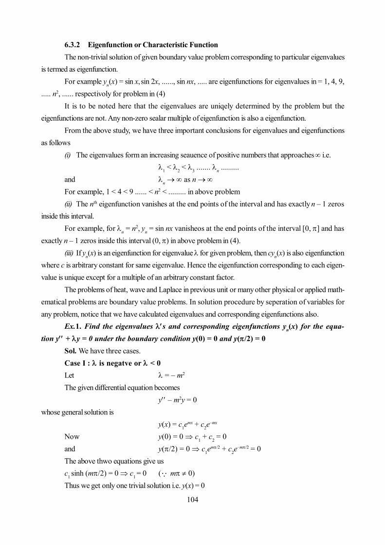
104
6.3.2 Eigenfunction or Characteristic FunctionThe non-trivial solution of given boundary value problem corresponding to particular eigenvalues
is termed as eigenfunction.For example yn(x) = sin x, sin 2x, ......, sin nx, ..... are eigenfunctions for eigenvalues in = 1, 4, 9,
..... n2, ...... respectivoly for problem in (4)It is to be noted here that the eigenvalues are uniqely determined by the problem but the
eigenfunctions are not. Any non-zero sealar multiple of eigenfunction is also a eigenfunction.From the above study, we have three important conclusions for eigenvalues and eigenfunctions
as follows(i) The eigenvalues form an increasing seauence of positive numbers that approaches i.e.
1 < 2 < 3 ....... n .........and n as n
For example, 1 < 4 < 9 ...... < n2 < ......... in above problem(ii) The nth eigenfunction vanishes at the end points of the interval and has exactly n – 1 zeros
inside this interval.For example, for n = n2, yn = sin nx vanisheos at the end points of the interval [0, ] and has
exactly n – 1 zeros inside this interval (0, ) in above problem in (4).(iii) If yn(x) is an eigenfunction for eigenvalue for given problem, then cyn(x) is also eigenfunction
where c is arbitrary constant for same eigenvalue. Hence the eigenfunction corresponding to each eigen-value is unique except for a multiple of an arbitrary constant factor.
The problems of heat, wave and Laplace in previous unit or many other physical or applied math-ematical problems are boundary value problems. In solution procedure by seperation of variables forany problem, notice that we have calculated eigenvalues and corresponding eigenfunctions also.
Ex.1. Find the eigenvalues s and corresponding eigenfunctions yn(x) for the equa-tion y + y = 0 under the boundary condition y(0) = 0 and y(/2) = 0
Sol. We have three cases.Case I : is negatve or < 0Let = – m2
The given differential equation becomesy – m2y = 0
whose general solution isy(x) = c1e
mx + c2e–mx
Now y(0) = 0 c1 + c2 = 0and y(/2) = 0 c1e
m/2 + c2e–m/2 = 0
The above thwo equations give usc1 sinh (m2) = 0 c1 = 0 ( m 0)Thus we get only one trivial solution i.e. y(x) = 0

105
Case II : when = 0The given problem reduces to
y = 0Hence the general solution is
y(x) = c1x + c2
So, under given boundary conditions, c1 = c2 = 0which gives trivial solution only i.e. y 0 for = 0Thus 0 are not eigenvalues for given problem.Case III : when is positive or > 0Let = m2
Then problem becomesy + m2y = 0 .....(6)
and y(0) = 0 and y(/2) = 0The general solution is y(x) = c1 sin mx + c2 cos mxWhen y(0) = 0, c2 = 0 and hence y(x) = c1 sin mxWhen y(/2) = 0, 0 = c1 sinn /2For seeking non-trivial solution, we should have c1 0 then sinn /2 = 0or sin m/2 = n; for some positive integer n
m/2 = n; n = 1, 2, 3, .... m = 2n; n = 1, 2, 3, .....
Therefore n = m2 = 4n2 ; n = 1, 2, 3, .....Hence n = 4, 16, 36, ........, 4n2 ...... are the increasing sequence of eigenvalues. The corre-
sponding eigenfunctions areyn(x) = sin 2nx; n = 1, 2, 3, ....
Ex.2. Find the eigenvalues and eigenfunctions for the boundary value problem y +y = 0 under the boundary condition y(a) = 0 and y(b) = 0, 0 < a < b; a, b are arbitrary realconstants.
Case I : < 0 or= – 2
Given problem reduces toy – 2y = 0
with y(a) = 0 and y(b) = 0The general solution is
y(x) = c1ex + c2e
–x
When y(a) = 0, c1ea + c2e
–a = 0 –c1e2a = c2
y(b) = 0, c1eb + c2e
–b = 0 –c1e2b = c2
Hence, –c1e2a = –c1e
2b
c1(e2a – e2b) = 0
Since a b, c1 = 0and hence c2 = 0
which implies y 0 i.e. only trivial solution exists.
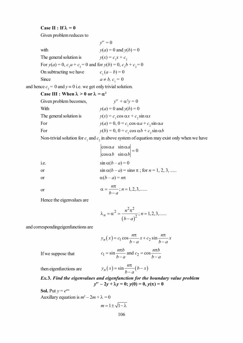
106
Case II : If = 0Given problem reduces to
y = 0with y(a) = 0 and y(b) = 0The general solution is y(x) = c1x + c2
For y(a) = 0, c1a + c2 = 0 and for y(b) = 0, c1b + c2 = 0On subtracting we have c1 (a – b) = 0Since a b, c1 = 0
and hence c2 = 0 and y 0 i.e. we get only trivial solution.Case III : When > 0 or = 2
Given problem becomes, y + 2y = 0With y(a) = 0 and y(b) = 0The general solution is y(x) = c1 cos x + c2 sin xFor y(a) = 0, 0 = c1 cos a + c2 sin aFor y(b) = 0, 0 = c1 cos b + c2 sin bNon-trivial solution for c1 and c2 in above system of equation may exist only when we have
cos sin0
cos sina ab b
i.e. sin (b – a) = 0or sin (b – a) = sinn ; for n = 1, 2, 3, .....or (b – a) = n
or ; 1, 2,3,......n nb a
Hence the eigenvalues are
2 22
2 ; 1, 2,3,......nn nb a
and correspondingeigenfunctions are
1 2cos sinnn ny x c x c x
b a b a
If we suppose that 1 2sin and cosn b n bc cb a b a
then eigenfurctions are sinnny x b x
b a
Ex.3. Find the eigenvalues and eigenfunction for the boundary value problemy – 2y + y = 0; y(0) = 0, y() = 0
Sol. Put y = emx
Auxillary equation is m2 – 2m + = 0
1 1m

107
Case I : If 1 – > 0 or< 1The general solution is
1 1 1 11 2
x xy x c e c e
Under given boundary conditions, y(0) = y () = 0, we havec1 = c2 = 0 or y 0
So, only trival solution exist i.e. < 1 does not give any eigenvalue.Case II : If 1 – = 0 or = 1The general solution of given problem is
y(x) = (c1x + c2) ex
On applying boundary conditions,y(0) = 0 and y() = 0 we have c1 + c2 = 0Hence, only trivial solution exists and therefore = 1 is not an eigenvalue.Case III : If 1– < 0 or > 1The general solution is
cos 1 sin 1 xy A x B x e
When y(0) = 0, we have A = 0 or y(x) sin 1 xB xe
For y() = 0, sin 1 0 since e 0 and B 0 for seeking non-zero solutions.Hence sin 1 = 0 = sin n, n = 1, 2, 3, .... – 1 = n2
or n = n2 + 1; n = 1, 2, 3, .....are required eigenvalues and corresponding eigenfunctions are
yn(x) = exsin nx n = 1, 2, 3, .....Ex.4. Find the eigenvalues and eigenfunctions for the following boundary value prob-
lemy – 4y + (4 – 9)y = 0, y(0) = 0, y(a) = 0,
where ‘a’ is a positive real constant.Sol. The auxillary equation of a given problem is
m2 + 4m + (4 – 9) = 0
4 16 4 4 9 2 3m
Case I : when = 0The general solution of given problem is
y(x) = e–2x (c1 + c2x)When y(0) = 0, c1 = 0or y(x) = c2xe–2x
Also when y(a) = 0, c2ae–2a = 0Since a > 0, therefore c2 = 0Hence, y 0 i.e. only trivial solution exists.

108
Case II : When > 0The general solution is
2 3 31 2
x x xy x e c e c e
On applying boundary conditiony(0) = 0, c1 + c2 = 0 or c2 = – c1
2 3 31
x x xy x c e e e
Again 2 3 310, gives 0a a ay a c e e e
c1 = 0 c2 = 0, y 0, only trival solution exists.For 0, the given problem has no non-zero eigenfunction.Case III : When < 0The general solution of given differential equation is
1 22 sin 3 cos 3 xy x e c x c x
Now y(0) = 0 gives c2 = 0
2 sin 3xy x e x
Also 210 gives sin 3 0ay a c e a
For non-trivial solution, we have c1 0, then
sin 3 0a
or sin 3 sin ; 1, 2,3, ....a n n
3na
or2 2
29n
a
Hence2 2
2 ; 1, 2,3.....9
nn na
are the required eigenvalues for given problem. Hence the corresponding eigenfunctions are
2 sin ; 1,2,3.....xn
n xy x e na
Ex.5. Find the eigenvalues and eigenfunctions for the following boundary value prob-lem
y – 3y + 2(1 + ) y = 0, y(0) = 0, y(1) = 0Sol. Auxillary equation for given differential equation is
m2 – 3m + 2(1 + ) = 0
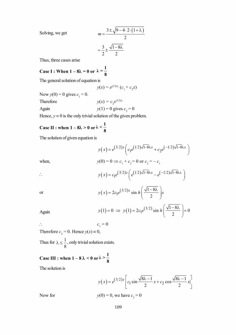
109
Solving, we get 3 9 4 2 12
m
3 1 82 2
Thus, three cases arise
Case I : When 1 – 8 = 0 or 1λ =8
The general solution of equation isy(x) = e(3/2)x (c1 + c2x)
Now y(0) = 0 gives c1 = 0.Therefore y(x) = c2x
(3/2)x
Again y(1) = 0 gives c2 = 0Hence, y 0 is the only trivial solution of the given problem.
Case II : when 1 – 8> 0 or1λ <8
The solution of given equation is
3 2 1 2 1 8 1 2 1 81 2
x x xy x e c e c e
when, y(0) = 0 c1 + c2 = 0 or c2 = – c1
3 2 1 2 1 8 1 2 1 81
x x xy x c e e e
or 3 21
1 82 sin2
xy x c e h x
Again 3 21
1 81 0 1 2 sin 02
y y c e h
c1 = 0Therefore c2 = 0. Hence y(x) 0,
Thus for 18
, only trivial solution exists.
Case III : when 1 – 8 < 0 or1λ >8
The solution is
3 21 2
8 1 8 1sin cos2 2
xy x e c x c x
Now for y(0) = 0, we have c2 = 0
110
3 21
8 1sin2
xy x c e x
Also 3 21
8 11 0 sin 02
xy c e
For seeking non-trivial solution, we have c1 0
therefore8 1sin 0
2
or8 1sin sin ;
2n
for positive integral n
2 28 1 4 18 1 2 ; 1,2,3,....
2 8nnn n n
are required eigenvalues and corresponding eigenfunctions are yn(x) = e(3/2)x sin nx (n N)
6.4 Sturm-Liouville Problem
A boundary value problem consisting of second order homogeneous linear differential equationof the form
0d dyp x q x r x ydx dx
.....(1)
where p, q and r are continuous real valued functions defined on a x b such that p has a continuousderivative, p(x) > 0 and q(x) > 0 and is a parameher independent of x and two homogenous bound-ary conditions
A1 y(a) + A2 y(a) = 0 .....(2)B1 y(b) + A2 y(b) = 0 .....(3)
where A1, A2, B1 and B2 are real constants such that A1 and A2 are not both zero and B1 and B2 are notboth zero simultaneously, is called Sturm-Liouville problem. All the problems we have discussed in pre-vious section are Sturm-Liouville problems.
Ex.1. Check whether the boundary value problemy – y = 0 with y(0) = 0 = y()
is Sturm-Liouville problem or notSol. On comparing with stanard form of Sturm-Liouville problem, we have
p(x) = 1, q(x) = 1, r(x) = 0, a = 0 and b = ;A1 = B1 = 1 and A2 = B2 = 0
Hence given problem is Sturm-Liouville problem.Ex.2. Check whether the following boundary value problem
xy + y + (x2 + 1 + ) y = 0y(0) = 0 and y(L) = 0, L is constant such that L > 1
is Sturm-Liouville problem or not.

111
Sol. xy + y + (x2 + 1 + ) y = 0(xy) + (x2 + 1 + ) y = 0
p(x) = x, q(x) = 1, r(x) = 1 + x2,a = 0 and B = L;A1 = 1, B1 = 0, A2 = 0 and B2 = 1
Since p(x) > 0 for 0 x LGiven boundary value problem is Sturm-Liouville problemEx.3. Find the eigenvalues and eigenfunctions of the following Sturm-Liouville prob-
lem
2x 2xd dye + λ +1 e y = 0;dx dxy(0) = 0 = y()
Sol. Transform dependent variable from y to u by using transformationy = e–xu
x xdy due e udx dx
Therefore given differential equation reduces to
2 21 0x x x x xd due e e u e e udx dx
22 x x xdue e e udx
22
2x x x x xdu d u due e e e u e
dx dxdx
+ e2x e–xu + e2x e–xu = 0
or2
2 0
x d ue udx
i.e. u + u = 0and boundary conditions reduce to
u(0) = 0 = u() since e–x 0 x Rwe know that n = n2; n = 1, 2, 3, ....
are the eigenvalues for reduced problem and corresponding eigenfunctions are un(x) = sin nx (see §6.3)Hence n = n2; n = 1, 2, 3, .... are the eigenvalues for given problem and corresponding
eigenfunctions areyn(x) e–x sin nx ; n N
Ex.4. Solve the following Sturm-Liouville problemy + y = 0; y(–) = 0, y() = 0
Sol. Let < 0 i.e. = –2
Then given problem becomesy – 2y = 0; y(–) = 0, y() = 0
112
The general solution is y(x) = c1 ex + c2e
–x
y(x) = c1ex – c2e–x
Now y(–) = 0 c1e–– c2e= 0and y() = 0 c1e– c2e–= 0For non-trivial solution for c1 and c2 for above system of equations, the coffecient determinant
must vanish. Hence
0e e
e e
– e– + e–= 0which is not possible. Hence c1= c2 = 0
Therefore only trivial solution exists that is y = 0When = 0.The general solution is y = c1 x + c2
So, y = c1
For boundary condition y(–) = 0 and y() = 0, c1= 0
Hence y (x) = c2 is solutionWhen > 0. Let = 2
Then given problem becomesy + y = 0
The general solution of the differential equation isy(x) = c1cos x + c2sin xy(x) = – c1sin x + c2cos x
An appling boundary condition y(–) = 0, we have c2 = 0 y(x) = – c1sin xAgain for y() = 0; –c1sin = 0Since c1 0; therefore sin = 0, i.e. sin = sin n; n =1,2,3, .....or = n ; n = 1,2,3, ..... n= n2 ; n = 1,2,3, .....are the required eigenvalues and corresponding eigenfunctions are yn(x) = cos nxHence from Case II and Case III, the eigenvalues for given problem are n = 0,1,4,9, .....n2 .....
and corresponding eigenfunctions are yn(x) = 1, cos x, cos2x, cos3x, .....cos nx, .....
6.5 Orthogonality of Eigenfunctions
From previous section, it is very much clear that the Sturm-Liouville problem is advanced boundaryvalue problem and have non-trivial solution if function p(x) and q(x) are restricted for p (x) > 0 andq (x) > 0 on [a, b] and iff the parameter takes a certain specific value. These are termed as eigenval-ues of boundary value problem. They are real numbers that can be arranged in an increasing sequence :

113
1 < 2 < ....... <n < n+1< ...... ....(1)and furthurmore n as n
This ordering is desirable to arrange corresponding eigenfunctionsy1 (x), y2 (x), ....., yn (x), yn+1 (x), ... .....(2)
in their own natural order. The eigenfunctions are not unique, but with the boundary conditions, they aredetermined up to a non-zero constant factor.
Now, we introduce a new concept in broader context that will assist to understand the propertyof various special functions that generally arise in various physical and engineering modelling.
A sequence of eigenfunctions yn (x) in (2) having the property
0
0b
m na n
if m ny x y x dx
if m n
is said to be orthogonal on the interval [a, b].If n = 1, n, the function yn (x) are said to be normalized and sequence of eigenfunctions is
known as orthonormal sequence.If sequence of eigenfunctions yn (x) have the following general property
0,
0,
bm na n
m nq x y x y x dx
m n
then, this sequence is said to be orthogonal with respect to a weight function q (x).
6.6 Important Theorems of Sturm-Liouville Systems
6.6.1 Theorem 1. The eigenvalues of Sturm-Liouville system are realProof. We have
0d dyp x q x r xdx dx
.....(1)
where a1 y (a) + a2 y(a) = 0, and b1y (b) + b2 y (b) = 0 ......(2)Suppose the p(x), q(x), r(x), a1, a2, b1 and b2 are real, while and y may be complex. Let
and y denote complex conjugates of and y respectively. Now we have from (1) and (2)
0d d yp x q x r xdx dx
.....(3)
where 1 2 0a y a a y a , and 1 2 0 b y b b y b . .....(4)Multiplying (1) by y and (3) by y and then subtracting we find that
d p x yy yy r x yydx
.....(5)
Integrating it from a to b and using boundary conditions (2) and (4), we find that
0 b
ar x yy dx .....(6)
Since r(x) is a non-negative and r(x) 0 for a x b, therefore (6) gives0 is real.
114
6.6.2 Theorem 2 : Let m and n be two distinct eigenvalues of the Sturm-Liouvilleproblem
0d dyp x q x r x ydx dx
.....(6)
and ym(x) and yn(x) be their corresponding eigenfunctions. Then ym(x) and yn(x) areorthogonal with respect to the weight function q(x) on the interval a x b.
Proof : If m and n are eigenvalues of given Sturm-Liouville problem
0 p x y x q x r x y x .....(7)
then we have
0 m m mp x y x q x r x y x .....(8)
and
0 n n np x y x q x r x y x .....(9)
On multiplying by (8) by yn and (9) ym respectively and on subtracting we get.
0 n m m n m n m ny x p x y x y x p x y x q x y x y x
m n m n m n n nq x y x y x y x p x y x y x p x y x
On integrating writh respect to x between a and b, we have
b b bm n m n m n n ma a a
q x y x y x dx y x p x y x dx y x p x y x dx
b bbm n m n m n m naa a
q x y x y x dx y x p x y x y x p x y x dx
bb
n m n ma ay x p x y x y x p x y x dx
bm n m n m n m na
q x y x y x dx y b p b y b y a p a y a
n m n my b p b y b y a p a y a
bm n m n m n n ma
q x y x y x dx p b y b y b y b y b m n n mp a y a y a y a y a
Now define w(x), a Wronskian determinant of the solution or eigenfunctions ym (x) and yn (x) as
m mm n n m
n n
y x y xw x y x y x y x y x
y x y x
So, expression (10) can be written as
b
m n m naq x y x y x dx p b w b p a w a .....(11)

115
For obtaining the orthogonality property
0b
m naq x y x y x dx for m # n
We seek right hand side of (10) or (11) to vanish, that isp(b) w(b) – p(a) w(a) = 0
This will certainly happen if the boundary conditions required for a non-trival solution of (7) are
0 and 0or
0 and 0
y a y b
y a y b
.....(12)
Above boundary conditions are special cases of more general boundary conditions.c1y(a) + c2y(a) = 0 and d1y(b) + d2y(b) = 0 .....(13)
where c1 and c2 donot vanish simultaneously and simillary d1 and d2 do not vanish simultaneously. Toverify that the general boundary condition in (13) really vanishes the right hand side of (11), Leteigenfunction ym(x) and yn(x) also satify boundary condition (13) i.e.
1 2 0m mc y a c y a
1 2 0n nc y a c y a
For non-trivial solution of c1 and c2 in above system of equations, the determinant
m m
n n
y a y aw a
y a y a
must vanish. Hence w (a) = 0. Simillarly w(b) = 0.So right hand side of (11) definitely vanishes and orthogonality of eigenfunctions is validated un-
der suitable boundary condition (13) which are homogeneous in nature. The problem (7) with boundarycondition (13) is known as Sturm-Liouville problem.
The significance of orthogonality property of eigenfunctions of Sturm-Liouville problem is to rep-resent series expansions of function f (x) in terms of eigenfunctions yn (x) as
f (x) = a1 y1 (x) + a2y2 (x) + ...... + an yn (x) + ...... .where the cofficient a1, a2 .... an, ..... can be derived using orthogonality property of eigenfunctions.6.6.3 Theorem 3 :To every eigenvalue of a Sturm-Liouville system there corresponds
only one linearly independent eigenfunction.Proof. Let if possible, y1 (x) and y2 (x) be two distinct eigenfunctions of the systems, corresponding
to same eigenvalue . In order to prove the linear independence of y1(x) and y2 (x), it is sufficient toprove that the wronskian
w (x) =
1 2
1 2
y x y x
y x y x is identically zero.
By definition,w (x) = 1 2 2 1y y y y

116
We have 1 2 2 1w x y y y y
and from the given boundary conditionsw (a) = w (b) = 0 .....(14)
Since y1(x) and y2(x) are solutions of Sturm-Liouville’s problem, therefore
1 1 0p y q r y
and 2 2 0p y q r y
Eliminating (q + r), we get
2 1 1 2 2 1 1 2 0y y y y p x y y y y p x
or 0p x w x p x w x
or 0 Cd p x w x w x
p x
Since p(x) 0, the boundary condition (14) gives C = 0 for all x. Hence w(x) 0 in [a, b],which means that, the eigenfunction y1(x) and y2(x) corresponding to same eigenvalue are linearly in-dependent.
6.6.4 Theorem 4 : (Expansion of a function in terms of eigenfunctions of Sturm-Liouvillesystem). If {n(x)} be a set of eigenfunctions of Sturm-Liouville system, then
1
n nn
A x
converges uniformly to a function f(x) in [a, b] such that
1
,n nn
f x A x a x b
.....(15)
where
2,
bma
m bma
r x f x x dxA m N
r x x dx
.....(16)
Proof. Without taking the proof of convergence, let f(x) is given by (15). Multiplying both sidesof (15) by r(x) m(x), integrating from a to b and changing the order of integration and summation (whichis justified due to uniform convengence of the series) we find that
1
b bm n n ma a
nr x f x x dx A r x x x dx
.....(17)
Since the set of eigenfunctions of Sturm-Liouville system are orthogenal in [a, b] w.r.t weightfunction r(x), therefore relation (17) reduces to
2 b b
m m ma ar x f x x dx A r x x dx
which gives Am given by (16).

117
Ex.1. Compute the eigenvalues and eigenfunctions for boundary value problem
y y y y2 1 0; 0 0 and y(1) = 0
Also prove that the set of eigenfunctions for the given problem is an orthogonal set.Sol. The auxillary equation is m2 + 2m + (1 – ) = 0
or 2 4 4 1
12
m
Now, three cases ariseCase I : When > 0 or = 2
The general solution of the given differential equation in this case will be
Now y (x) = 1 11 2
xxc e c e
For y (0) = 0 c1 + c2 = 0 or c2 = – c1
1 11
x xy x c e e
Now y (1) = 0 gives 1 11 0c e e
c1 = 0Hence c2 = 0 = c1 y(x) 0 i.e. only trivial solution exists.Case II : When = 0 :The general solution is y(x) = e–x (c1 + c2 x)For y (0) = 0, we get c1 = 0. Hence y (x) = c2xe–x
When y (1) = 0, we get c2 e–1 = 0 c2 = 0.
Thus c1 = c2 = 0, which gives y 0 i.e. only trivial solution exists.Case III : When < 0 or = – 2
Then general solution is
y (x) = 1 2cos sinxe c x c x For y (0) = 0, we have c1 = 0
So 2 sinxy x c e x
Now, for y(1) = 0, we have 12 sin 0c e
For seeking non-trivial solution of given problem, we have c2 0, so sin 0
or sin sin ;n n is positive integer
n
– = n22
l n= – n22 ; n = 1, 2, 3, ...... .Hence, corresponding eigenfunctions are
yn (x) = e–x sin nx

118
Let ym (x) = e–x sin mx and yn (x) = e–x sin nx are two eigenfunctions corresponding to eigen-values m = – m22 and n = – n2 2 resectively. Then the integral
1 20
xm ne y x y x
1 20
sin sin x x xe e m x e n x dx
1
0sin sinm x n x dx
1
0
1 cos cos2
m n x m n x dx
1
0
sin sin12
m n x m n xm n m n
= 0prompts that ym (x) and yn (x) are orthogonal in [0, 1] with respect to weight function e2x.
Self-Learning Exercise
1. Classify the following problem as boundary value problem or initial value problem(a) y – y = 0, y(0) = 0 and y(1) = 0(b) y + 2y + 2y = 0, y(0) = 1(c) (xy) + (9 + 4) y = 0, y(a) = 0, and y(b) = 0, a, b are constonts(d) 3y + 4y + 2y = 0, y(2) = 5, y(2) = 6
2. Find the eigenvalues n and eigenfunctions yn(x) for y + y = 0 in each of the following bound-ary conditions(a) y(0) = 0, y(1) = 0(b) y(–2) = 0, y(2) = 0(c) y(–3) = 0, y(0) = 0(d) y(1) = 0, y(4) = 0
3. Check whether following boundary value problems are Sturm-Liouville problem or not(a) exy + exy + y = 0; y(0) = 0, y(1) = 0
(b) y + (1 +x)y = 0; y(0) = 0, y(2) + y(2) = 0
(c) 1
y
x + (x + ) y = 0; y(0) + 3y(0) = 0, y(1) = 0
(d) (xy) + (x2+ 1 – x2)y = 0; y(0) = 0; y(0) + 3y(0) = 0, y(1) + y(1) = 0
(e) (xy) + (x2+ 1 + ex)y = 0; y(1) = 0; y(1) + 2y(1) = 0; y(2) – 3y(2) = 0
4. Find eigeavalues and corresponding eigenfunction of the following Sturm-Liouville problems.
(a) y+ y = 0; y (0) = 0 and y() = 0
(b) y+ y = 0; y (0) = 0 and y(L) = 0
(c) y+ y = 0; y (–) = 0 and y() = 0

119
6.7 Summary
In this unit, we introduced a special type of boundary value problem known as Sturm-Liouvilleproblem which gives fundamental basics for important concepts like eigenvalue, eigenfunction, orthogo-nality and Fourier series. These concepts directly involved in solving practical problems arise in physicaland engineering challenges.
6.8 Answer to Self-Learning Exercise
1. (a) Boundary value problem(b) Initial value problem(c) Boundary value problem(d) Initial value problem
2. (a) 2 2 ; 1, 2,3...... sinn nn n y x n x
(b) 2 2
; 1,2,3...... sin16 4n n
n nn y x x L
(c) 2 2
; 1, 2,3...... sin9 3n n
n n xn y x
(d) 2 2
; 1, 2,3...... sin 49 3n n
n nn y x x
3. (a) Yes (b) Yes(c) No, since p(x) is not continuous in [0, 1](d) No, since q(x) < 0 in [0, 1](d) Yes
4. (a) 22 1 2 1; ,1,2,3....., sin
4 2
n nn nn y x x
(b) 2 2
2cos; 0,1, 2,3.....,n n
n n xn y xLL
(c) 2; 1, 2,3....., cosn nn n y x nx
6.9 Exercise
1. Find the eigenvalues n and eigenfunction yn (x) for the following boundary value problem0y y in each of the following boundary conditions :
(a) y (0) = 0, y (2) = 0 [Ans. 2
; 1,2,3,......, sin4 2n nn nxn y x ]
(b) y (0) = 0, y (L) = 0 ; L > 0, L is positive constant
[Ans. 2 2
2 ; 1, 2,3,......, sinn nn n xn y x
LL
]

120
(c) y (–L) = 0, y (L) = 0 ; L > 0, L is positive constant
[Ans. 2 2
2 ; 1,2,3,......, sin24n n
n x Ln n y xLL
]
2. Solve the following Sturm-Liouville problem
(a) 0; 1 0, 0d dyx y y y edx dx x
[Ans. 2 ; 1,2,3,......, sin ln | |n nn n y x n x ]
(b) 221 0;
1
d dyx ydx dx x
y(0) = 0 and y(1) = 0 (Hint put x = tan t)
[Ans. 2 116 ; 1,2,3,......, sin 4 tann nn n y x n x ]
3. Compute the eigenvalues and eigenfunctions for boundary value problem and determine Euclid-ean space in which a complete set of eigenfunctions for the given problem is an orthogonal set
(a) 1 0; 0 0, 0y y y y
[Ans. 2 1n n ; n = 1, 2, 3, ....., yn (x) = sin nx orthogonal in [0,]
(b) 4 4 1 0, 1 0, 1 0y y y y y
[Ans. 2 2n n , yn (x) =
2
2
sin ; 2, 4,6......2
cos ; 1,3,5......2
x
x
n xe n
n xe n
Orthogonal in (–1, 1) with resepect to function e–x ]
(c) 2 1 0; 0 0y y y y and 0y
[Ans. n = – n2 ; n = 1, 2, 3, ..... ., yn = e–x (n cos nx + sin nx), n = 1, yn = 1. Orthogonal in[0, ] with respect to weight function e2x ]
4. Find the real eigenvalues and eigenfunctions for the boundary value problem 0y y ;
y (0) = 0, 1 0y [Ans. 2 20 00; 1; , cos ,n ny x n y x n x n N ]
5. Find the solution of Sturm-Liouville problem 21 0, 1 2y y y xx x
with boundary conditions 1 0 2y y [Ans. 1
logsinlog 2n
n
xy B n
]
7. Determine the normalized eigenfunctions of the problem 0y y , y(0) = 0, 1 1 0y y .
Hence expand the function f (x) = x, 0 1x , in terms of these normalized eigenfunctions.
[Ans. 1 2
2 21
4sin2 sin , , sin1 cos 1 cos
nn n n
nn n n
y x x n N x x
]

121
Unit 7 : Variational Problems with Fixed Boundaries andEuler-Lagrange Equation
Structure of the Unit
7.0 Objective
7.1 Introduction
7.2 Definitions and Fundamental Problems
7.2.1 Functionals
7.2.2 Linear Functionals
7.2.3 Brachistochrone Problem
7.2.4 Problem of Geodesics
7.2 Isoperimetric Problem
7.3 Euler-Lagrange Equation
7.3.1 Basic Lemma
7.3.2 Euler-Lagrange Equation
7.4 Some Elementary Cases of Integrability of Euler-Lagrange Equation
7.4.1 F is independent of y
7.4.2 F is independent of x and y.
7.4.3 F is independent of only y.
7.4.4 F is a linear function of y.
7.4.5 F is independent of only x
7.5 Variational Problems for Functionals Involving Several Dependent Variables and Their First
Order Derivatives.
7.6 Summary
7.7 Answers to Self-Learning Exercise
7.8 Exercise
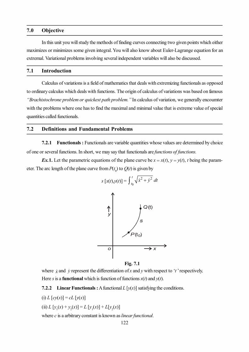
122
7.0 Objective
In this unit you will study the methods of finding curves connecting two given points which eithermaximizes or minimizes some given integral. You will also know about Euler-Lagrange equation for anextremal. Variational problems involving several independent variables will also be discussed.
7.1 Introduction
Calculus of variations is a field of mathematics that deals with extremizing functionals as opposed
to ordinary calculus which deals with functions. The origin of calculus of variations was based on famous
“Brachistochrone problem or quickest path problem.” In calculus of variation, we generally encoumter
with the problems where one has to find the maximal and minimal value that is extreme value of special
quantities called functionals.
7.2 Definitions and Fundamental Problems
7.2.1 Functionals : Functionals are variable quantities whose values are determined by choice
of one or several functions. In short, we may say that functionals are functions of functions.
Ex.1. Let the parametric equations of the plane curve be x = x(t), y = y(t), t being the param-
eter. The arc length of the plane curve from P(t0) to Q(t) is given by
s [x(t),y(t)] = 0
2 2t
tx y dt
P (t )
Q (t)
0
s
xo
y
Fig. 7.1where x and y represent the differentiation of x and y with respect to ‘t ’ respectively..Here s is a functional which is function of functions x(t) and y(t).
7.2.2 Linear Functionals : A functional L [y(x)] satisfying the conditions.
(i) L [cy(x)] = cL [y(x)]
(ii) L [y1(x) + y2(x)] = L [y1(x)] + L[y2(x)]
where c is a arbitrary constant is known as linear functional.
123
Ex.2. 0
,x
x
dyL y x a x b x y dxdx
is a linear functional.
The calculus of variations provides a method for determining maximal and minimal values offunctionals. Such problems are known as variational problems.
Now we deal with three problems of historical importance which influenced the development ofthis subject.
7.2.3 Brachistochrone ProblemSuppose P and Q are two points in the plane but not in the same vertical line. Imagine, there is a
thin flexible wire connecting those two points. Suppose P is above Q, and we let a frictionless beadtravel under gravity from P to Q. The Bachistochrone problem (or quickest discent problem) is con-cerned with determining the path of the bead when it reaches the point Q in the least possible time. Thisproblem was first introduced by J. Bernaulli in the mid of 17th century and was first solved by Sir IsaacNewton.
7.2.4 Problem of GeodesicsIn general relativity, a geodesic generalizes the concept of straight line to curve spacetime. For
example : Find the curve of shortest length connecting two points in space. If there is no constraints thesolution obviously is a straight line joining the points. However, if the curve is constrained and is to lie ona surface, then in space, the solution is less obvious and possibly many solutions may exist.
The solutions are called geodesics. In other words a geodesics on a surface is a curve alongwhich the distance between two points on the surface is a minimum. To find the geodesics on a surfaceis a variational involving conditional extremum.
7.2.5 Isoperimetric ProblemIn this problem, we required to find a closed plane curve of a given length l bounding a maximal
area S. Let the parametric equation of the plane curve be x = x(t) , y = y(t), and the curve is traversedonce in anti-clockwise as t increases from t0 to t1, then length l of given curve is
1
0
2 2t
t
l x t y t dt ......(1)
which is a constant, and enclosed area is given by
0
12
t
t
S xy yx dt .....(2)
The problem is to maximize the functional S, given by (2) subject to the condition that the lengthl of the curve given by (1) must have a constant value.
7.3 Euler-Lagrange Equation
7.3.1 Basic Lemma : Let M(x) be a continuous function on the internal [a, b]. Suppose
that for any continuous function h(x), we have 0b
a
M x h x dx then M(x) 0 on the inter-
val [a,b].

124
Proof : Let M(x) 0 (say positive) at a point x where a x b. Since M(x) is continuouson [a, b], it follows that if M(x) 0. Then M(x) maintains its sign in a certain neighbourhood x0 x x1
of the point x .Since h(x) is arbitrary continuous function, we may choose h(x) s.t. h(x) remains positive in
x0 x x1 while it vanishes outside the interval. Hence, we obtain.
1
0
0xb
a x
h x M x dx h x M x dx .....(1)
Since the product h(x)M(x) remains positive in [x0, x1] and vanishes outside this interval.
By the hypothesis 0b
a
h x M x dx .....(2)
which contradicts (1). This contradiction shows that our assumption M(x) 0 at some point xmust be wrong and so M(x) 0 on [a, b].
7.3.2 Euler-Lagrange Equation : If y(x) is a curve in interval [a, b] which is a twice
differentiable and satisfying the conditions y(a) = y1 and y(b) = y2 and minimizes the functional.
, ,b
a
F y x f x y y dx .....(3)
where dyydx
.
Then the following differential equation must be satisfied
0f d fy dx y
.....(4)
Proof. Suppose y y(x) is a curve which minimizes the functional F. That is, for any permissiblecurve y = g(x), F[y(x)] F[g(x)]. We have to construct a function of one real variable satisfying follow-ing properties.
1. H() is a differentiable near = 02. H(0) is a local minimum for H.We begin by constructing a variation of y(x). Let be a small real number (positive or
negative). s.t.
y x y x h x
where h(x) is a continuous function in [a, b] and h(a) = h(b) = 0.
y
xx = a x = bo
Fig. 7.2
125
We can define a function H to be
H F y x Since y(x) minimizes F(y(x)), it follows that it minimizes H(). Since H(0) is minimum value of
H, we know that from ordinary calculus that H(0) = 0.The function H can be differentiated by using Leibnitz rule, that is
, ,b
a
d dH f x y y dxd d
, ,b
a
f x y y dx .....(5)
Now applying chain rule within the integral, we abtain
y yf f x f fx y y
y yf fy y
f fh x h xy y
Substituting the value of f
in the equation (5), we have
b
a
dH f fh x h x dxd y y
Using H(0) = 0, we find that
0 0b
a
f fH h x h x dxy y
Integrating by parts, we get
0 0bb b
a a a
f f d fH h x dx h x h x dxy y dx y
0bb
aa
f d f fh x dx h xy dx y y
0b
a
f d f h x dxy dx y
[Using h(a) = h(b) = 0]
By using lemma, we conclude that
0f d fy dx y
.....(6)
126
This equation is called Euler-Lagrange equation.
7.3.5 Remark : The statement of the lemma and its proof donot change if restriction h(a) =
h(b) = 0 is imposed on the function h(x).
7.4 Some Elementary Cases of the Integrability of the Euler-Lagrange Equation
7.4.1. f is independent of y : If f is independent of y, then f is function of (x, y) only. There-
fore 0fy
. Thus the Euler-Lagrange equation reduces to following form :
0fy
.....(1)
Now integrating (1), with respect to y, we obtain a arbitrary curve f = g(x), without any con-stant and in general, does not satisfy boundary conditions y(a) = y1 and y(b) = y2. Thus this type ofequation does not posses a solution.
7.4.2. f is indpendent of x and y : In this case,
2 20f f f f
x y x y y y
.....(2)
From Euler-Lagrange equation
0f d fy dx y
, we get
2 2 2
2 0f f f fy yy x y y y y
, ,f f x y y
From equation (2), we have2
2 0fyy
.....(3)
This implies that either y = 0 or 2
2 0fy
Now y = 0 y = Ax + B .....(4)
where A and B are arbitrary constants, which is a two parameter family of straight lines. But if 2
2 0fy
has one or several real roots y = Kn, then y = Knx + c
which is one parameter family of straight line contained in two parameter family of straight lines. Thus
extremals are all possible straight lines.
7.4.3. f is indpendent of only y : Here f f(x, y), therefore Euler-Lagrange equation can be
written as

127
0d fdx y
as 0fy
f cy
.....(5)
where c is a constant. Since this relation is independent of y it can be solved for y as a function of x.
Another integration leads to a solution involving two arblitraray constants which can be obtained by
using given boundary conditions.
7.4.4. f is a linear function of y or f is binearly dependent on y such that f(x, y, y) =
p(x, y) + q(x,y)y
Forming the Euler-Lagrange equation for this particular f, we have
0p q dq p q q q p qy y yy y dx y y x y y x
.....(7)
for all x and y.Solution of this problem, in general, not possible because solution does not satisfy given bound-
ary conditions. But if we consider 0p qy x
, then the expression pdx + qdy becomes exact differen-
tial equation whose solution does not depend on path of extremal and therefore variational becomes
meaningless.
Ex.1. Test for an extremum of the functional
1
2 2 2
0
, 0 0, 1 1F y x x y x y dx y y .....(8)
Sol. Clearly we see that
2 2 2, ,f x y y x y x y
is a linear function of y. Now from case 7.4.4, we have p(x,y) = x2y2, q(x,y) = x2
Hence from equation (7), we find that
0p qy x
2x2y – 2x = 0
2x (xy-1) = 0
xy =1 or x = 0
Obviously first boundary condition is satisfied by only x = 0, by and second boundary condition
is satisfied by only xy = 1. Both boundary conditions are not satisfied by the curves x = 0 and xy =
1.Thus no solution exist for this problem.

128
Ex.2. Test for extremum of the functional
cos sinb
a
F y x y xy y dx .....(9)
with boundary conditions y(a) = y0, y(b) = y1
Sol. For this problem, Euler-Lagrange equation is given by
sin cos sin 0dy xy y x ydx
or sin cos sin cos 0y xy y y xy y
Thus, integrand being an exact differential equation. Therefore variational problem becomes mean-ingless
7.4.5. f is independent of x : In this case, 0fx
, therefore Euler-Lagrange equation re-
duces to
0d ff ydx y
Hence Euler-Lagrange equation has its integral as ff y cy
where c is arbitrary constant
Ex.1. Test for extremum of the functional
1
2
0
1 F y x y dy= , y(0) = 0, y(1) = 2
Sol. Using Euler-Lagrange equation, we get
2
2 01
d ydx y
Integrating with respect to ‘x’, we get
21
y cy
, where c is arbitray constant
2
2 say1
cy Ac
Again integrating with respect to ‘x’
y = Ax + B
y(0) = 0 and y(1) = 2, implies that B = 0, A = 2
Thus y = 2x which is a straight line.

129
Ex.2. Test for extremum of the functional
1
2 2
0
, 0 1, 1 2F y x y x dx y y
Sol. Using Euler-Lagrange equation, we get
0f d fy dx y
2 0d ydx
yIntegrating two times we get y = Ax + BUsing y(0) = 1, y(1) = 2, we get A = B = 1.Thus solution is y = x + 1.Ex.5. (Brachistochrone problem or quickest descent problem)Find the shape of the curve on which a bead is sliding from rest and accelerated by
gravity will ship (without friction) in least time from one point to another.Sol. Let us consider a particle P descending from A(0,0) to B(a,b) under gravity along some
curve. We have to determine shape of the curve which gives minimum possible time to descent. LetP(x,y) be the position of the particle at any time t and having actual arc length s from a point A.
A (0, 0 )
P x, y ( )
B a, b ( )
s
x
y
Fig. 7.3Under the gravity, the motion of particle is given by
2ds gydt
2dsdty g
Hence time T of descent is (from A to B).
0 2
a dsTy g
.....(10)
But we know that
2
1ds dydx dx

130
21ds y dx where dyydx
Putting the value of ds in equation (10), we obtain
2
0
12
a yT dxgy
Here f(x, y, y) = 21
2y
gy f(x)
Now from case (7.4.5), we have
1fy f cy
2
12
1 122 1
y yy cgygy y
22
1
1c
y y
(where 2 12c g c )
or 231y y c 2
3 2where 1c c
Now putting 2 33cot sin 1 cos 2
2cy y c
Since dy ydx
dydxy
32 cos sincot
c ddx
23 32 sin 1 cos 2dx c d c
Integrating we get
33 4 4
sin 2 2 sin 22 2
cx c c c
and 3 1 cos22cy
If we substitute 2 = , and using intial condition (that is at A(0,0)), we have
c4 = 0 ; and 3 sin2cx , and 3 1 cos
2cy
which is equation of the cycloid with radius 3
2c of rolling circle and c3 can be obtained by using
appropriate boundary condition.

131
Ex.4. (The minimal surface of revolution problem)Find the curve with fixed boundary revolves such that its rotation about x-axis gener-
ate mininal surface area.Sol. We know that, surface area of the relvolution is given by
2b
a
S y x y ds
22 1b
a
y y dx
Here f(x,y, y ) = 2y 21 y f(x)
From case (7.4.5), the first integral of Euler’s equation is
1ff y cy
22
12
22 11
yyy y cy
221
y cy
(where 1
2 2cc
)
2 22
dydxy c
Integrating with respect to ‘y’ we get
12 3
2cosh yx c c
c
32
2cosh x cy c
c
where c2 and c3 are arbitrary contestants, which is a equation of the “catenary” and the corre-sponding surface of revolution is called “centroid” of revolution.
7.5 Functionals Involving Several Dependent Variables and Their First Order De-
rivatives.
We now proceed to derive the differential equations that must be satisfied by the twice differen-tiable functions x1(t), x2(t), ...., xn(t) that extremize the integral
2
1
1 2 1 2, ,..... , , ,..... ,t
n nt
I f x x x x x x t dt

132
with respect to those functions of x1, x2, ...., xn which achieve prescribed values at the fixed limits ofintegration t1 and t2, where t1 < t2. The superior dot represents ordinary differentiation with respect tothe independent variable t.
We denote the set of actual extremizing functions by x1(t), x2(t), ...., xn(t) and proceed to formthe one-parameter family of comparison functions
X1(t) = x1(t) +1(t), X2(t) = x2(t) +2(t) ,....., Xn(t) = xn(t) +n(t) .....(2)where 12nare arbitrary differentiable functions for which1(t1) = 1(t2) = 2(t1) = 2(t2) = ....= n(t1) = n(t2) = 0 .....(3)
and is the parameter of the family. The condition (3) assures us that every member of each compari-son family satisfies the required prescribed end point conditions. We see, moreover, that no matter whatthe choice of 12n, the set of extremizing functions x1(t), x2(t), ...., xn(t) is a member of eachcomparison family for the penameter value = 0. Thus if we form the integral.
2
1
1 2 1 2, ,....., , , ,....., ,t
n nt
I f X X X X X X t dt .....(4)
by replacing x1, x2, ...., xn etc, in (4) by X1, X2, ...., Xn etc., respectively, we have that I(0) is the extre-mum value sought. We therefore conclude that
0 0I .....(5)
It follows from (2) that
1 1 1 2 2, , ....,n n n nX x X X X x .....(6)Now differentiate (4) with respect to ‘’, we have
2
1
1 1 2 21 1 2 2
..... ,t
n nn nt
dI f f f f f f dtd X X X X X X
.....(7)
where we use (2) and (6) to derive the sequence of substitution 11,....., n
nXX
.
It is clear from (2) and (6) that setting = 0 is equivalent to replaeing X1,X2, ....., Xn, 1 2, ,....., nX X X
by x2, x2, ...., xn, 1 2, ,..... nx x x respectively. Thus because of (5), we abtain from (7) on setting = 0
2
1
1 1 2 21 1 2 2
0 ..... 0t
n nn nt
f f f f f fI dtx x x x x x
.....(8)
This last relation holds for all choices of the functions 1(t),2(t), ...., n(t). In particular, it holdsfor the special choice in which 2, ...., nare identically zero, but for which 1(t) is still arbitrary, consis-tent with (3). With this selection of 1,2, ...., nwe integrate by parts the second term of the secondmember of (8) to obtain, since 1(t1) = 1(t2) = 0,
2
1
11 1
0t
t
f d f dtx dt x
.....(9)
133
Since (9) holds for all, 1 we conclude by applying the basic Lemma that
1 10f d f
x dt x
.....(10)
Through similar treatment of the successive pairs of terms of the second member of (8) we de-rive like equations, with x1 replaced by x2, ...., xn, Joining these equations with (10), we have
1 1 2 20, 0,....., 0
n n
f d f f d f f d fx dt x x dt x x dt x
.....(11)
for the system of simultaneaes Euler-Lagrange equations which must be satisfied by the functions x1(t),x2(t), ....., xn(t) which render the integral (1) an extremum.
Ex.1. Find the extremals of the functional
2
2 2
0
2
π
I y, z = y + z + yz dt
with the boundary conditions y(0) = 0, y() = –1 ; z(0) = 0, z() = 1Sol. Here 2 2 2f y,z, y,z ,t y z yz
Then from equation (11), we can see that
0f d fy dt y
0f d fz dt z
or 0y z and 0z y .....(12)Eliminating ‘z’ from this system, we get
0ivy y or 4
4 0d y ydt
Its solution is given byy = c1 e
t + c2 e–t + c3 cost + c4 sint .....(13)
where c1, c2, c3 and c4 are arbitrary constants. Now from equation (12) we have
1 2 3 4cos sint tz y c e c e c t c t .....(14)
Applying the given boundary conditionsy(0) = 0, y() = –1, z(0) = 0, z() = 1, we find thatc1 = c2 = c3 = 0, c4 = –1.
Hence the extremal curve is the intersection of the surfacesy = – sin t, z = sin t.
Ex.2. (a) Find the extremum of the function
2
1
12 21x
x
yF y x dx
x
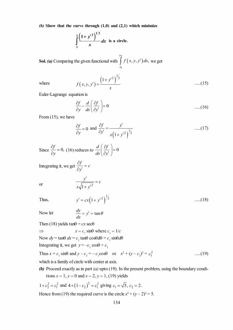
134
(b) Show that the curve through (1,0) and (2,1) which minimize
1 222
1
1 ydx
x
is a circle.
Sol. (a) Comparing the given functional with 2
1
, , ,x
x
f x y y dx we get
where
12 21
, ,y
f x y yx
.....(15)
Euler-Lagrange equation is
0f d fy dx y
.....(16)
From (15), we have
0fy
and
12 21
f yy x y
.....(17)
Since 0,fy
(16) reduces to 0d fdx y
Integrating it, we get f cy
or 21
y cx y
Thus, 1
2 21y cx y .....(18)
Now let tandy ydx
Then (18) yields tan = cx sec x = c1 sin where c1 = 1/cNow dy = tan dx = c1 tancosd = c1 sindIntegrating it, we get y = –c1 cos + c2
Thus x = c1 sin and y – c2 = – c1cos or x2 + (y – c2)2 = 2
1c .....(19)
which is a family of circle with center at axis.(b) Proceed exactly as in part (a) upto (19). In the present problem, using the boundary condi-
tions x = 1, y = 0 and x = 2, y = 1, (19) yields2 22 11 c c and 2 2
2 14 1 c c giving 1 25, 2c c .
Hence from (19) the required curve is the circle x2 + (y – 2)2 = 5.
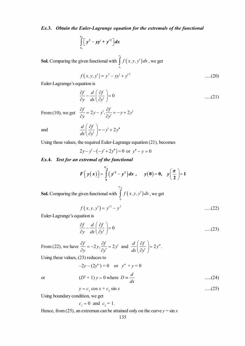
135
Ex.3. Obtain the Euler-Lagrange equation for the extremals of the functional
2
1
2 2x
x
y yy + y dx
Sol. Comparing the given functional with 2
1
x
x
f x, y, y dx , we get
2 2f x, y, y y yy y .....(20)Euler-Lagramge’s equation is
0f d fy dx y
.....(21)
From (10), we get 2 2f fy y , y yy y
and 2d f y ydx y
Using these values, the required Euler-Lagrange equation (21), becomes
2 2 0y y y y or 0y y
Ex.4. Test for an extremal of the functional
2
2 2
0
0 0 12
F y x y y dx , y , y
Sol. Comparing the given functional with 2
0
f x, y, y dx
, we get
2 2f x, y, y y y .....(22)Euler-Lagrange’s equation is
0f d fy dx y
.....(23)
From (22), we have 2 , 2 and 2 .f f d fy y yy y dx y
Using these values, (23) reduces to
–2y – (2y) = 0 or y+ y = 0
or (D2 + 1) y = 0 where dDdx
.....(24)
y = c1 cos x + c2 sin x .....(25)Using boundary condition, we get
c1 = 0 and c2 = 1.Hence, from (25), an extremun can be attained only on the curve y = sin x

136
Self-Learning Exercise
1. Is 0
2 is linear ? Yes / No.x
x
L y x y dx
2. Is 0
2
2 is linear ? Yes / No.x
x
d yL y x c x y dxdx
3. As extremal of the functional
, , ,b
a
F y x f x y y dx y(a) = y1 , y(b) = y2 satisfies Euler-Lagrange equation,
which in general is a(a) linear second order ODE(b) admits a unique solution(c) non-linear ODE of order greater than two.(d) may not admit a solution.
4. The curve of shortest distance between two fixed points is(a) straight line(b) circle(c) parabola(d) none of these
5. The Euler-Lagrange equation for a functional of the form ,b
a
f x y dx is
(a) fy = c1
(b) fy – yfy= c1
(c) fy = c1(d) none of these
6. The extremizing curve of the brachistochrone problem is a(a) circle(b) catenary(c) cycloid(d) straight line.
7.6 Summary
The caluclus of variation, which plays an important role in both pure and applied mathematics,
dates from the time of Newton. Development of the subject started mainly with the work of Euler andLagrange. In this unit we have solved a number of problem of engineering and physics with the help ofEuler-Lagrange equations.

137
7.7 Answers to Self-Learning Exercises
(1) No (2) Yes
(3) (d) (4) (a)
(5) (d) (6) (a)
7.8 Exercise
1. Find the extemal of the function 1 2
0
1 ,yI y x dxy
throught the origin and the point (1, 1).
[Ans. y = tan(x/4)]2. (a) Show that if y satisfies the Euler-Lagrange’s equation associated with the integral
2
1
2 2 2 2x
x
I p y q y dx
where p(x) and q(x) are known functions, then I has the value 2
1
2 x
xp yy
(b) Show that, it y satisfies the Euler-Lagrange’s equation associated with part (a) and if z(x) is anarbitrary differentiable function for which z(x1) = z(x2) = 0
then 2
1
2 2 0x
x
I p y z q yz dx
3. Prove that the extremal of 1 221b
a
y y is the catenary y = a cos h(ax + b)
4. Prove that the extremal of 2 2
0
y dxx
with y(0) = 0 and y(2) = 1 is a parabola.
5. Prove that the extremals of
2
1
2 2x
x
I u x y x y dx
subject to the condition that
2
1
2x
x
J x y dx k (a constant)
are the solution of Sturm-Liouville equation
0d dyu x x x y ,dx dx
with y(x1) = y(x2) = 0

138
6. Show that the extremum of the functional
2
1
2 2 2 sinx
x
I y y y x dx,
is given by 1 21 sin2
x xy c e c e x
7. Show that the Euler’s equation for the functional
21b
a
I f x, y y dx has the form 2 01
yy x ,y
ff f
y
8. Find an extremal to
2 2
1
11 0 2 1
yI dx, y , y
x
[Ans. x2 + (y – 2)2 = 5]
9. Find the curve y = (x) which corresponds to the extreme value of
2b
n
a
dyF y x x dxdx
[Ans. 1
12 1
1
nc xy c , nn
1 2log 1c x c , n ]
10. Show that the curve of shortest distance (geodesic) on a right circular cylinder is a Helix or agenerator.
11. Find the extremals of the functional 2 2 22 2b
a
F y x ,z x yz y y z dx
Deduce the extremals if a = 0, b = ; 0 0 1 0 0 1y , y , z , z .
[Ans. 1 2 3 4cos siny c x c x c c x 1 2 3 3 4 12 cos 2 sinz c x c c x c c c x ]

139
Unit 8 : Functionals Dependent on Higher Order Derivativesand Variational Problems in Parametric Form
Structure of the Unit
8.0 Objective
8.1 Introduction
8.2 Variational Problems Involving Several Higher Order Derivatives
8.3 Variational Problems Involving Functionals Dependent on the Functions of Several Independent
Variables and Dependent Variable
8.4 Variational Problems in Parameteric Form
8.5 Isoperimetric Problem
8.6 Summary
8.7 Answers to self-learning Exercise
8.8 Exercise
8.0 Objective
This unit deals with the functionals dependent on higher order derivatives and functions of morethan one independent variable. The variational problems in parametric form are also included in the presentunit.
8.1 Introduction
In the previous unit, we have discussed the Euler-Lagrange’s equation and various variationalproblems having their first order derivatives. In this unit, we will disuss the variational problem with func-tional dependent on higher order derivatives, several independent variables and variational problem inparametric form.
8.2 Varitional Problems Involving Several Higher Order Derivatives
Theorem : If the function f contains higher order derivatives, say upto any order n, then
, , , ...., nf f x y y y .....(1)
and we need to extremize the integral
2
1
, , , ...x
n
x
I f x y y y dx .....(2)
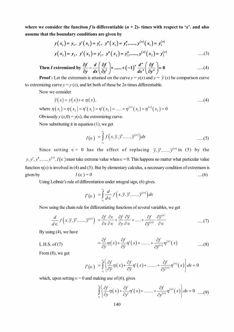
140
where we consider the funciton f is differentiable (n + 2)- times with respect to ‘x’. and alsoassume that the boundary conditions are given by
1 1 1 1 1 1 1 1
n ny x y , y x y , y x y , ....., y x y
2 2 2 2 2 2 2 2
n ny x y , y x y , y x y , ....., y x y .....(3)
Then I extremized by 1 0n
nn n
f d f d f......y dx y dx y
.....(4)
Proof : Let the extremum is attained on the curve y = y(x) and y = y (x) be comparison curveto extremizing curve y = y (x), and let both of these be 2n times differentiable.
Now we consider
y x y x x , .....(4)
where 1 2 1 2 1 2 0n nx x x x ..... x x
Obviously y (x,0) = y(x), the extremizing curve.Now substituting it in equation (1), we get
I
2
1
xn
x
f x, y , y ,....., y dx .....(5)
Since setting = 0 has the effect of replacing ny , y ,....., y in (5) by the ny, y , y ,....., y ,I must take extreme value when = 0. This happens no matter what particular value
function (x) is involved in (4) and (5). But by elementary calculus, a necessary condition of extremum isgiven by I () = 0 ....(6)
Using Leibniz’s rule of differentiation under integral sign, (6) gives.
I
2
1
xn
x
d f x, y , y ,....., y dxd
Now using the chain rule for differentiating functions of several variables, we get
nd f x, y , y ,....., yd
n
n
f x f y f y.....x y y
.....(7)
By using (4), we have
L.H.S. of (7) n
n
f f fx x ........ xy y y
.....(8)
From (8), we get
I
2
1
0x
nn
x
f f fx x ........ x dxy y y
which, upon setting = 0 and making use of (6), gives
2
1
0x
nn
x
f f fx x ........ x dxy y y
.....(9)

141
where we have used the fact that when = 0, n ny y, y y ,....., y y .
Now integrating by parts, we have
2
1
x
x
f xy
2 2
11
x x
xx
f d fx x dxy dx y
2
1
x
x
d f x dxdx y
and 2
1
x
x
f x dxy =
2 2
11
x x
xx
f d fx xy dx y
2
1
x
x
d f xdx y
.....(10)
Again integrating with respect to ‘x’ we get
2
1
x
x
y x dxy
2 2
11
2
2
x x
xx
d f d fx x dxdx y dx y
Thus, 2
1
x
x
f x dxy
2
1
2
2
x
x
d f x dxdx y
Similarly
2
1
xn
nx
f dxy
2
1
1x n
nn n
x
d f x dxdx y
...(11)
Using it in equation (9), we obtain
2
1
2 1 0x n
nn n
x
f d f d f d f.......... xy dx y dx y dx y
which gives
2 1 0n
nn n
f d f d f d f...y dx y dx y dx y
.....(12)
8.3 Variational Problem Involving Functionals Dependent on the Functions of
Several Independent Variables and Dependent Variables
In this section, we will discuss the variational problems which is dependent on several depen-dent and independant variables.
Theorem : If z is a curve which is dependent on x, y and is twice differentiable in itsdomain D, and extremize the functional
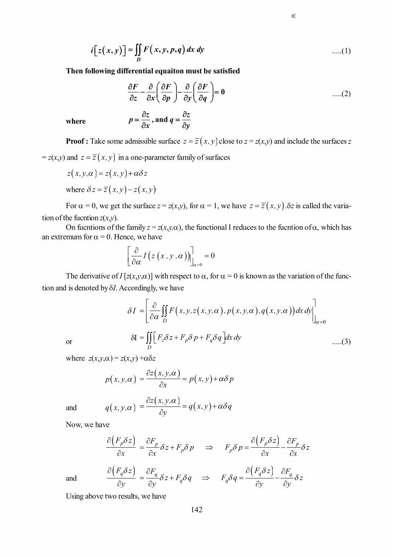
142
,i z x y , , ,D
F x y p q dx dy .....(1)
Then following differential equaiton must be satisfied
0F F Fz x p y q
.....(2)
where andz zp , qx y
Proof : Take some admissible surface z z x, y close to z = z(x,y) and include the surfaces z
= z(x,y) and z z x, y in a one-parameter family of surfaces
z x, y, z x, y z
where z z x, y z x, y
For = 0, we get the surface z = z(x,y), for = 1, we have z z x, y z is called the varia-tion of the fucntion z(x,y).
On fucntions of the family z = z(x,y,), the functional I reduces to the fucntion of which hasan extremum for = 0. Hence, we have
0
0I z x , y ,
The derivative of I [z(x,y,)] with respect to , for = 0 is known as the variation of the func-tion and is denoted by I. Accordingly, we have
I 0D
F x, y,z x, y, , p x, y, ,q x, y, dx dy
or z p qD
F z F p F q dx dy .....(3)
where z(x,y,) = z(x,y) +z
p x, y, z x, y,
p x, y px
and q x, y, z x, y,
q x, y qy
Now, we have
pF zx
pp p
p pF zF F
z F p F p zx x x
and qF z
y
qq q
q qF zF F
z F q F q zy y y
Using above two results, we have
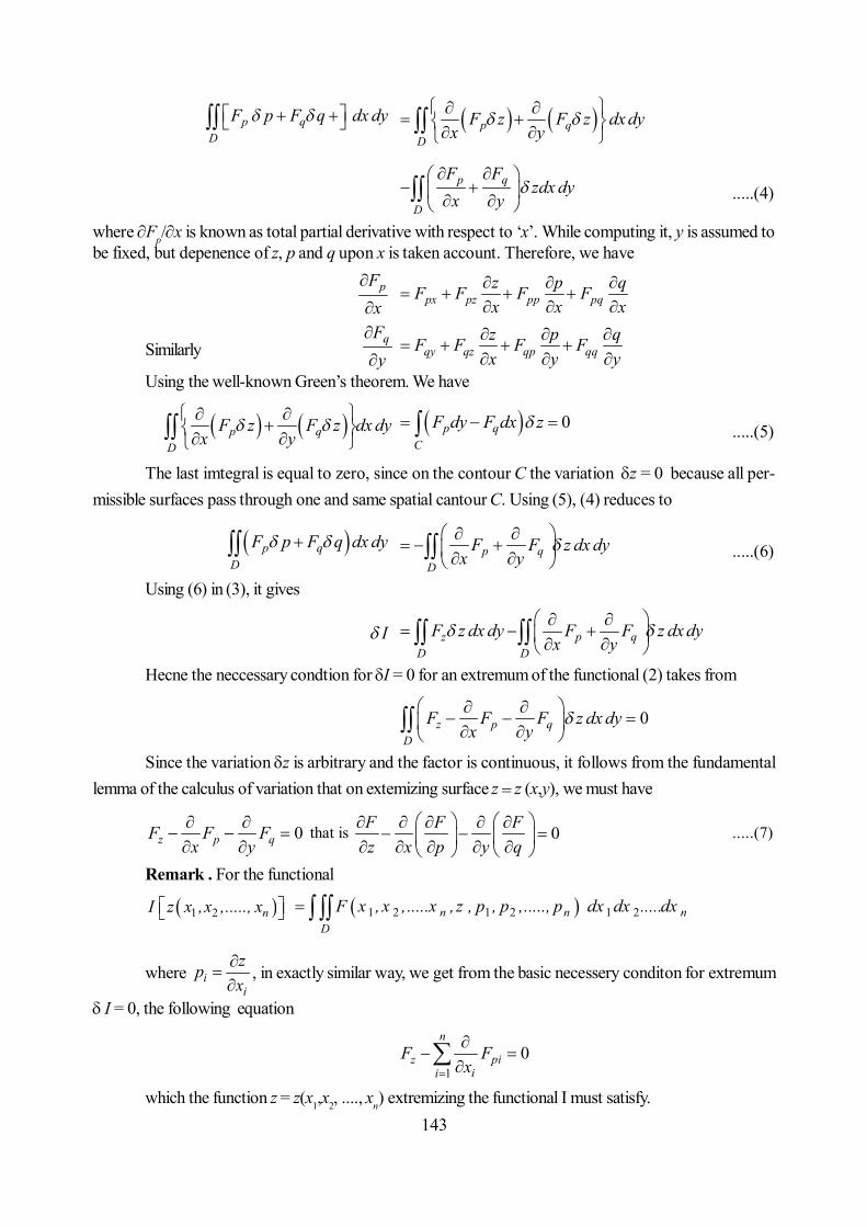
143
p qD
F p F q dx dy p qD
F z F z dx dyx y
p q
D
F Fzdx dy
x y
.....(4)
where Fp/x is known as total partial derivative with respect to ‘x’. While computing it, y is assumed tobe fixed, but depenence of z, p and q upon x is taken account. Therefore, we have
pFx
px pz pp pqz p qF F F Fx x x
SimilarlyqF
y
qy qz qp qqz p qF F F Fx y y
Using the well-known Green’s theorem. We have
p qD
F z F z dx dyx y
0p q
C
F dy F dx z .....(5)
The last imtegral is equal to zero, since on the contour C the variation z = 0 because all per-missible surfaces pass through one and same spatial cantour C. Using (5), (4) reduces to
p qD
F p F q dx dy p qD
F F z dx dyx y
.....(6)
Using (6) in (3), it gives
I z p qD D
F z dx dy F F z dx dyx y
Hecne the neccessary condtion for I = 0 for an extremum of the functional (2) takes from
0z p qD
F F F z dx dyx y
Since the variation z is arbitrary and the factor is continuous, it follows from the fundamentallemma of the calculus of variation that on extemizing surface z = z (x,y), we must have
0z p qF F Fx y
that is 0F F Fz x p y q
.....(7)
Remark . For the functional
1 2 nI z x ,x ,....., x 1 2 1 2 1 2n n nD
F x , x ,.....x , z , p , p ,....., p dx dx .....dx
where ii
zpx
, in exactly similar way, we get from the basic necessery conditon for extremum
I = 0, the following equation
10
n
z piii
F Fx
which the function z = z(x1,x2, ...., xn) extremizing the functional I must satisfy.

144
8.4 Variational Problems in Parameteric Ferm
In some problems, the requirement of single valuedness is excessively restrictive; for it turns outthat Euler-Lagrange’s equation-derived under assumption that the extremizing function is single valued-may have for the solution which satisfies the given end point conditions, a relationship in which depen-dent variable is not a single valued function of the independent variable. One cannot, without furtherjustificaiton, accept such a solution as valid.
We proceed to show, that the extremizing relationship between a pair of variables x and y is thesame, whether the solution is derived under the assumption that y is a single valued function of x or thata more general parametric representation is required to express the relation between x and y. We do thisby showing that the solution of Euler-Lagrange equation derived on the basis of the assumption of thesingle valuedness of y as a funciton x satisfies also the system of Euler-Lagrange’s equations derived onthe basis of the parametric relationship between x and y.
Under the assumption that y is a single valued funciton of x, the integral to be extremized is givenas
I 2
1
x
x
f x, y, y dx .....(1)
where y is required to have values y1 and y2 at x = x1 and x = x2. If instead, we use the parametricrepresentation x = x(t), y = y(t) where x(tj) = xj and y(tj) = yj for j = 1,2, the integral (1) transformedto through the relationships
ydy ydx x
and dx = x dt .....(2)
where the supirior dot represents differntiation with respect ot ‘t’ .
Therefore I2
1
t
t
yf x, y, x dtx
.....(3)
The Euler-Lagrange’s equation for (1) is
0f d fy dx y
.....(4)
According to § 7.5, the system of Euler-Lagrange’s equation assiociated with (3) can be writtenas
g d gx dt x
0 0g d g,y dt y
where g x, y,x, y f x, y, y x .....(5)
From (5), we obtain
g f gx,x x x
2
f y ff x f yy yx
.....(6)

145
With the aid of second relation of (2), we obtain
d g d fx f ydt x dx y
f d f fx yy dx y x
.....(7)
Further, we obtain from (5)g f gx,y y y
1f fx
y x y
.....(8)
According to the second relation of (5), we have
d gdt y
d fxdx y
.....(9)
Combining this last result with the first of (8), we obtain the pair of equations
g d gx dt x
g d gy ,y dx y
g d gy dt y
g d gxy dx y
.....(10)
From this result, we conclude that any relationship, single-valued or not, that satisfies the Euler-Lagrange’s equaiton (4), derived on the basis of an assumed single valued solution y = y(x), satisfiesalso the system (5), whose derivation requires no assumption of single-valuedness of y as function of x.
8.5 Isoperimetric Problem
In this section, we seek to derive the differentiable equation which must be satisfied by the funcitonwhich renders the integral
I b
a
f x, y, y dx .....(1)
an extremum with respect to continuously differentiable functions y = y(x) for which the second integral.
J b
a
g x, y, y dx .....(2)
possesses a given prescribed value, and with y(a) = y1, y(b) = y2 both prescribed boundary conditionsThe given functions f and g are twice differentiable with respect to x.
To solve this type of problem, we will use the method of Lagrange’s multiplier. But first of all,we need to choose suitable extremizing function for this problem. If we choose Y(x) = y(x) + (x)which is a function of one perameter family. Then it yields the problem, because any change of the valueof the single perameter would in general alter the value of J, whose constancy must be maintained asprescribed. For this reason we introduce the two perameter family
Y(x) = y(x) + (x) + (x) .....(3)in which , and are arbitrary differentiable function for which (a) = (a) = 0 and (b) = (b) =0. These conditions ensures that Y(a) = y(a) = y1 and Y(b) = y(b) = y2 as prescribed, for all values ofparameters and
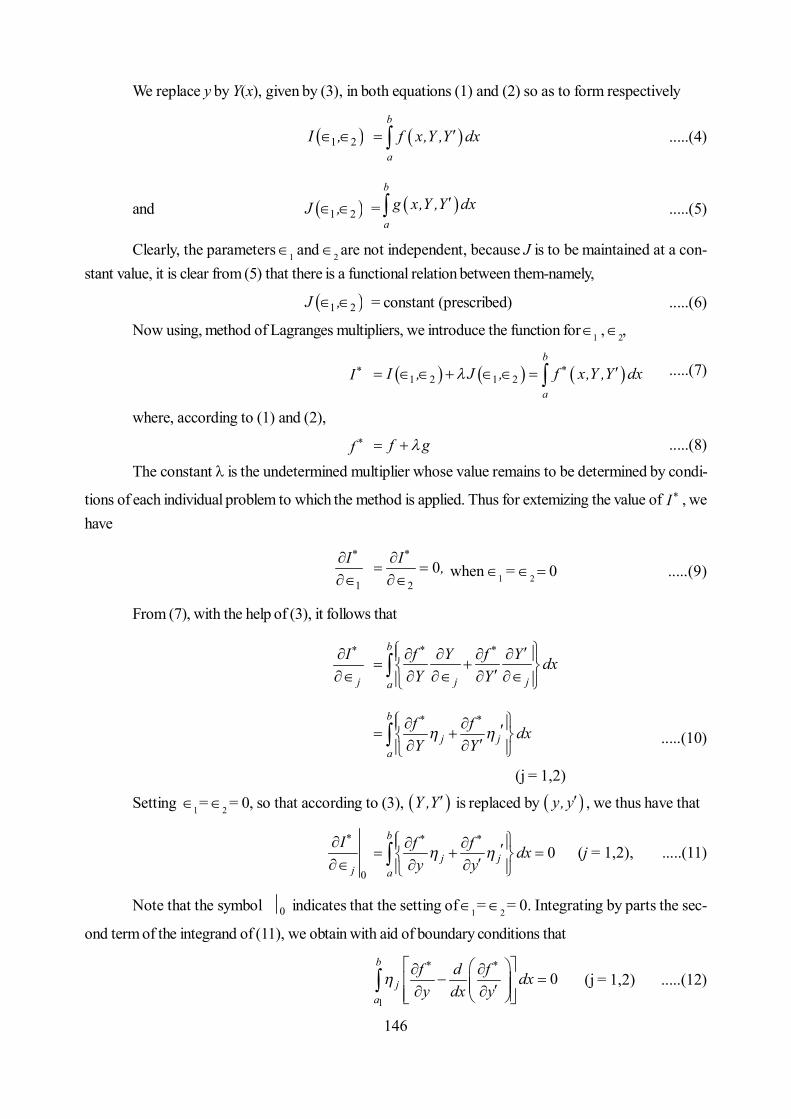
146
We replace y by Y(x), given by (3), in both equations (1) and (2) so as to form respectively
1 2I , b
a
f x,Y ,Y dx .....(4)
and 1 2J , = b
a
g x,Y ,Y dx .....(5)
Clearly, the parameters and are not independent, because J is to be maintained at a con-stant value, it is clear from (5) that there is a functional relation between them-namely,
1 2J , = constant (prescribed) .....(6)
Now using, method of Lagranges multipliers, we introduce the function for ,
I 1 2 1 2
b
a
I , J , f x,Y ,Y dx .....(7)
where, according to (1) and (2),
f f g .....(8)
The constant is the undetermined multiplier whose value remains to be determined by condi-
tions of each individual problem to which the method is applied. Thus for extemizing the value of I , wehave
1
I 2
0I ,
when =
From (7), with the help of (3), it follows that
j
I
b
j ja
f Y f Y dxY Y
b
j ja
f f dxY Y
.....(10)
(j = 1,2)
Setting = = 0, so that according to (3), Y ,Y is replaced by y, y , we thus have that
0j
I
0b
j ja
f f dxy y
(j = 1,2), .....(11)
Note that the symbol 0 indicates that the setting of = = 0. Integrating by parts the sec-
ond term of the integrand of (11), we obtain with aid of boundary conditions that
1
0b
ja
f d f dxy dx y
(j = 1,2) .....(12)

147
Now using basic lemma, we obtain the differential equation
0f d fy dx y
.....(13)
as the Euler-Lagrange’s equation which must be satisfied by the function y(x) which extrimizes (1) underthe restriction that (2) be maintained at a prescribed value.
Ex.1. Find the extremal of the functional
I 1
2
0
1= y dx ,
under the conditions 0 0 0y = , y 1 1 1 1 1= , y = , y =
Sol. In this problem,
, , ,f x y y y 21 y Therefore, the extremal function is given by solution of the following differential equation
2
2 0f d f d fy dx y dx y
2
20 0 2 0d ydx
4
4 0d ydx
.....(14)
The solution of differential equation (14) isy = c1 + c2x + c3x
2 + c4x3
Using the given conditions we easily obtain y = xThus extremal curve is a straight line.Ex.2 . Find the extremal of the functional.
I y x π
22 2 2
0
= dx,y - y + x
0 1 0 0y = , y = , π2y π0 12= , y = .
Sol. Comparing the given functional with
I y x π
2f x, y, y , y dx
0
=
we get f x, y, y , y 2 2 2y y x .....(15)Using equation
2
2 0f d f d fy dx y dx y
.....(16)

148
From (15) we getfy
2 , 0, 2f fy yy y
So (16) reduces to
2
22 2 0dy ydx
or 2
4 0d y ydx
or (D4–1)y = 0 where dDdx
.....(17)
The auxilliay equation of (17) is
m4 – 1 = 0 m = 1, i
Thus solution of (17) is y = c1ex + c2e
–x + c3cosx + c4 sin x .....(18)
Using boundary conditions y(0) = 1, y(2) = 0, we get
c1+ c2+ c3 = 1 .....(19)
and 2 21 2 4c e c e c
0 .....(20)
Since 0 0y and 12y therefore we find that
c1– c2+ c4 = 0 .....(21)
2 21 2 3c e c e c
1 .....(22)
Adding (19) and (22), we get
2 21 21 1c e c e
0
and subtracting (20) from (21), we get
2 21 21 1c e c e
0
Above two relations give c1 = c2 = 0 and using it in (19) and (21), we getc4 = 0, c3 = 1
Hence extremum can be attained only on the curve y = cosxEx.3 . Find the extremal equation for the following functional
1 2, I z x x 11 2
2 2
2D
=z z dx dxx x
Sol. Here the integrand f is a function of two independent variables x1 and x2 , i.e.
1 21 2
z zF z, , , x ,xx x
2 2
1 2
z zx x
.....(23)
Therefore, using the result
1 1 2 20F F F
x p x p z
.....(24)
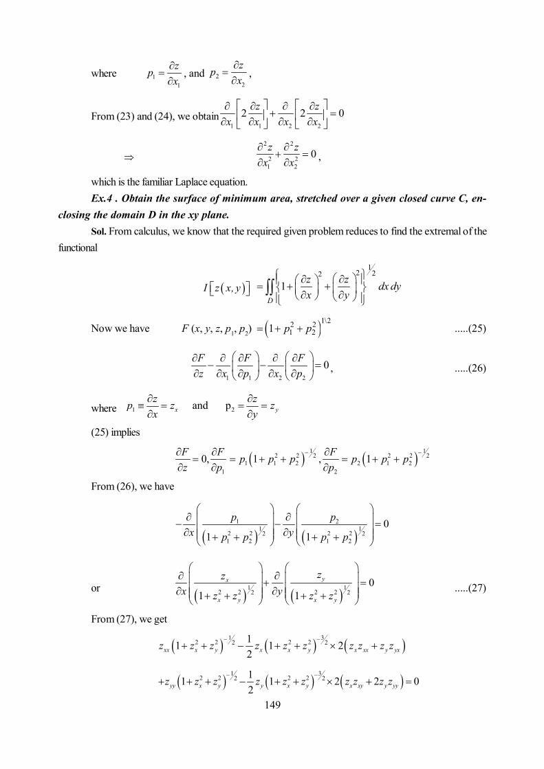
149
where 11
zpx
, and 22
zpx
,
From (23) and (24), we obtain1 1 2 2
2 2 0z zx x x x
2 2
2 21 2
0z zx x
,
which is the familiar Laplace equation.Ex.4 . Obtain the surface of minimum area, stretched over a given closed curve C, en-
closing the domain D in the xy plane.Sol. From calculus, we know that the required given problem reduces to find the extremal of the
functional
I z x, y
12 22
1D
z z dx dyx y
Now we have F (x, y, z, p1, p2) 1\22 21 21 p p .....(25)
1 1 2 2
0F F Fz x p x p
, .....(26)
where 1 2and px yz zp z zx y
(25) implies
1
0,F Fz p
1 12 2 2 22 2
1 1 2 2 1 22
1 , 1Fp p p p p pp
From (26), we have
1 2
1 12 2 2 22 21 2 1 2
01 1
p px yp p p p
or 1 1
2 2 2 22 20
1 1
yx
x y x y
zzx yz z z z
.....(27)
From (27), we get
31
2 2 2 22 211 1 22xx x y x x y x xx y yxz z z z z z z z z z
31
2 2 2 22 211 1 2 2 02yy x y y x y x xy y yyz z z z z z z z z z

150
or 22
1 2 3 2 1 2 3 22 2 2 2 2 2 2 2
1 1
1 1 1 1yx
xx yy
x y x y x y x y
zzz zz z z z z z z z
3 22 2
20
1x y xy
x y
z z z
z z
or 2 21 1 2 0xx y yy x x y xyz z z z z z z
That is
2 22 2 2
2 21 1 2 0z z z z z z zx y y x x y x y
whose solution will yield the desired minimal surface.Ex.5 . Find the closed convex curve of length L that encloses greatest possible area.Sol. We know that the area of the closed plane curve is given by the integral
I 12
b
a
xy yx dt .....(27)
where x ,dx dyydt dt
.
The total length of the curve is, given by
L1
2 2 2b
a
x y dt .....(28)
has the same value L where L is the length of the plane curve. Now the question is to maximize (extremize)(27) under the restriction (28), We will use the equation (13) of (§ 8.5), which is given below :
f d fx dt x
0 , 0f d fy dt y
.....(29)
where f 2 212
xy yx x y .....(30)
From (29) and (30), we have
2 2
1 1 02 2
d xy ydt x y
2 2
1 1 02 2
d yx xdt x y
From which we obtain, by direct integration with respect to ‘t’,
2 2
xyx y
1 22 2, yc x c
x y
......(30)

151
From these, we have
2 21 2y c x c
2 22 2
2 2
x yx y
Thus we have the well-known result “that the closed curve of given perimeter for which theenclosed area is a maximum is a circle.”
Ex.6 . (Shape of hanging rope). Find the shape assumed by a uniform rope when sus-pended by its end from two points. at equal heights.
Q a( , 0)
1
y
x
Fig. 8.1Sol. Let the rope of lenght 2L be suspended between two points P(–a,0) and Q(a,0) in the
same straight line, as points are at equal heights.Thus if denotes the constant mass per unit length of rope, the potential energy of an element of
length ds at (x, – y) is given by (–gy ds) where g is the constant acceleration due to gravrity. Accord-ingly, the total potential energy of the rope in the arbitrary configuration y = y(x) is given by
I 21a a
a a
g y ds g y y dx
.....(31)
where prime represents the differentiation with respect to ‘x’. and taking absolute value.According to minimum energy principle the equillibrium configuration is supplied by particular
relation y = y(x) for which (31) is a minimum with respect to functions y(x) for which y(a) = 0, y(–a) =0, and for which the total length of arc
J 21 2a
a
y dx L
.....(32)
We may therefore apply the Euler-Lagrange equation to the integrand function
f 2 21 1gy y y .....(33)
formed from (31) and (32). Since f is explicitly independent of the variable x, however, we may useEuler-Lagrange equation and so substitute (30) into (13) (§ 8.5), we easily abtain.
2
212
11
ygy y cy

152
2
11 y
1cgy
21 y 2
21
gyc
2y 2
21
1gy
c
y 2 2
121
gy cc
1
2 21
c dy dxgy c
Putting g y += c1cos ht and integrating, we find that 11
21
cosc gyh c xg c
Solving we get
y 21
1
coshg x cc
g g c
.....(34)
where c2 is an arbitrary constant of integration.Thus, according to (34), the shape of a hanging rope is that of a catanary with vertical axis. By
specifying that catenry passing through (–a,0) and (a,0) and that arc included between these points havelength 2L, we may assign value to constants c1, c2, . appearing in (34).
Ex.7 . Determine the curve of prescribed lengh 2l which joins the points (–a,b) and (a,b)and has its centre of gravity as low as possible.
Sol. Let P1 P2 be an are joining the given paints (–a,b) and (a,b). The y-coordinate of the centreof gravity of the required curve is given by
I 1
2 21 12
a
aaa
a
a
y dsy y dx
lds
where we have used the given constraint; namely
1
2 21a a
a a
ds y dx
2l , that is 1
2 21 1 12
a
a
y dxl
.....(35)
The boundary conditions are y(–a) = b, and y(a) = b
Let F x, y, y 1 1
2 22 21 12 2y y yl l

153
1
2 212
yy
l
where is the Lagrange’s multiplier. Since F does not contain x, thus from Euler-Lagrange’s equation
FF y cy
(a constant)
or
1 22 2
1 22
1
2 2 1
y y y y cl l y
.....(36)
or
11 221
yc
y
where c1 = 2cl. Re-writing the above equation we have
21 y 2
21
yc
or
22 21
21
y cdydx c
Separating variables and then integrating, we get
x
1 21 22 21
dyc c
y c or 1
1 21
cosh yx c cc
So that y 21
1cosh x cc
c
.....(37)
which is a complete solution of equation (36) on [–a,a] and boundary condition will be satisfied by thissolution if and only if
1
bc 2
1cosh a c
c
and 2
1 1cosh a cb
c c
that is to say if and only if (a + c2)/c1 = (a – c2)/c1
Hence c2 = 0. Thus equation (37) reduces to 11
cosh xy cc
.....(38)
This shows curve must be symmetric with respect to y-axis. Thus, we get.
1 1cosh ac c b / .....(39)Using (38) in (35), we get
1 221
1 1 sinh 12
a
a
x c dxl
or 1cos 2a
a
h x c dx l
or 1 1 1 12 sin ( ) 2 sin ( )c h a c l l c a c
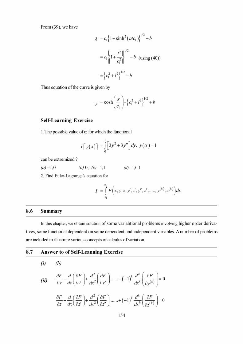
154
From (39), we have
1 221 11 sinhc a c b /
1 22
1 21
1 lc bc
(using (40))
1 22 21c l b
Thus equation of the curve is given by
y 1 22 21
1cosh x c l b
c
Self-Learning Exercise
1.The possible value of for which the functional
I y x 1
2
0
3 3 1y y dy, y
can be extremized ?
(a) –1,0 (b) 0,1(c) –1,1 (d) –1,0,1
2. Find Euler-Lagrange’s equation for
I 2
1
xk k
x
F x, y,z , y ,z , y ,z ,....., y ,z dx
8.6 Summary
In this chapter, we obtain solution of some variabtional problems involving higher order deriva-
tives, some functional dependent on some dependent and independent variables. A number of problems
are included to illustrate various concepts of calculus of variation.
8.7 Answer to of Self-Leanning Exercise
(i) (b)
(ii)
2
2 ....... 1 0k
kk k
F d F d F d Fy dx y ydx dx y
2
2 ....... 1 0k
kk k
F d F d F d Fz dx z zdx dx z

155
8.8 Exercise
1. Show that the Euler’s equation for the surface area functional
I u 2 21 x yu u dx dy
is 2 21 2 1 0y xx x y xy x yyu u u u u u u
2. Find the Euler’s equation for the functional.
I 2 2 2x yu u f x, y u x, y dx xy
where is a closed region in the xy-plane and u has continuous partial derivatives.
[Ans : 2 2
2 2 ]z z f x, yx y
3. Find the general solution of the extremals
(i)2 2 2
2 2D
p xy qx y dx dy
(ii) 2
D
xyz ypq xp dx dy
where p z x , q z y [Ans : (i) z = c1(y) log x + c2 (y) + (x3/9)
(ii) z = c1(y) – {–c2(y)/2x2} + (yx2/15)]
4. Find the extremal for the functional
I x t , y t 2
1
1 22 2 2 t
t
x y a xy yx dt
where a being a constant. [Ans : circles]
5. Find the extremal of the functional
I x t , y t 4
2 2
0
2 2xy x y dt ,
subject to the initial conditions at t = 0, x = y = 0; at 4
t x = y = 1.
[Ans.sin 2
sin 2h tx y
h ]
6. Find the curve of length L that join the paints (0, 0) and (1, 0) lie above the x-axis, and encloses
the maxinmm area between itself and x-axis.
156
[Ans. 2 2 21 1x c y c where
1 22
1 21 12 4
c ,c
and is the solution of 1 sin
2 2L
]
7. Find the extremals of the isoperimetric problem
1
2 2
0
I y x y x dx, given that 1
2
0
2 0 0 1 0y dx ; y , y .
[Ans. y = sin mx , m = 1,2,3]8. Find the curve joining two points (x1,y1) and (x2,y2) that yields a surface of revolution of station-
ary area when revolved about the x-axis. [Ans. a circle]
157
Unit 9 : Series Solution of Second Order Linear DifferentialEquation
Structure of the Unit
9.0 Objective
9.1 Introduction
9.2 Power Series Method
9.2.1 Validity of the Power Series Method
9.2.2 Definitions
9.2.3 Radius of Convergence
9.3 Series Solution Near an Ordinary Point
9.4 Series Solution Near a Regular Singular Point
9.4.1 Working Rule
9.5 Series Solution in Descending Powers of the Independent Variable
9.6 Self-Learning Exercise
9.7 Summary
9.8 Answers to Self-Learning Exercise
9.9 Exercise
9.0 Objective
The main object of this unit is to find the solution of a linear differential equation of second orderwith variable coefficients in terms of a series near ordinary and singular points with special reference toGauss hypergeometric equation and Legendre equation.
9.1 Introduction
We know about the methods of solving linear differential equations of second order with con-stant coefficients and in certain cases with variable coefficients. But sometimes, in case of variable coef-ficients the problem becomes intricate and we are not able to find the solution in a closed form. Undersuch situation, we can find a power series in terms of the independent variable x satisfying certain condi-tions. This method is called the method of solution in series or integration in series. Legendre’s equa-tion, Hypergeometric equation and Bessel’s equation are the examples whose solutions have been ex-pressed in the form of a infinite power series eg. the general solution of y + y = 0 is y = a cos x + bsin x and this may be rewritten as

158
2 4 3 51 ... ...
2 4 3 5x x x xy a b x
This shows that the general solution of the linear differential equation may be expressed by thesuperposition of a pair of infinite series.
9.2 Power Series Method
The basic concept of power series method is simple and we will apply this technique to the so-lution of some second order differential equations.
Let us consider the differential equation
2
2 0d y dyP x Q x R x ydxdx
.....(1)
where P(x), Q(x) and R(x) are polynomial in x and P(x) 0.The above equation may be written as
2
1 22 0d y dyp x p x ydxdx
.....(2)
where p1(x)
2, andQ x R x
p xP x P x
To find the solution of the equation (1), we assume a series for y of the form
y = a0 + a1x + a2x2 + ...
0
rr
ra x
.....(3)
Now substituting the values of y, dydx
and 2
2d ydx
in equation (2) and rearranging the terms of
different powers of x, we get an algebraic equation of the type
0 + 1x + 2x2 + ... = 0 .....(4)
Since equation (4) holds good for all values of x, identically, we obtain
0 = 0 , 1 = 0, 2 = 0 ,..., n = 0 ...
From these equations, we can determine the coefficients a0, a1, a2 ... etc. Putting the values of
a0, a1, a2, ... in the equation (3), we get the required solution which will be clear from the followingexample.
Ex.1. Solve in series
2
221 2 2 0d y dyx x y
dxdx
Sol. Let the solution of the equation bey = a0 + a1x + a2x
2 + ... .....(5)
dydx
= a1 + 2a2x + 3a3x2 + ...

159
and2
2d ydx
= 2a2 + 6a3x + 12a4x2 + ...
Substituting the values of y, dydx
and 2
2d ydx
in the given differential equation and simplifying, we
get2a0 + 2a2 + 6a3x + (12a4 – 4a2)x
2 + (20a5 – 10a3)x3 + ... = 0
Equating to zero, the coefficients of various powers of x, we obtain
a2 = – a0, a3 = 0, 024 5, 0
3 3aaa a
Substituting for as in equation (5), we get4
21 0 1 ....
3xy a x a x
which is the required solution.
9.2.1 Validity of The Power Series Method
In general an infinite series of the form
20 0 1 0 2 00
....rr
ra x x a a x x a x x
is called a power aseriesLet us consider a differential equation
2
2 22 2 0d y dyx x x y
dxdx
If we assume a solution of the formy = a0 + a1x + a2x
2 + ...and solve the equation by the above method, we find that
a0 = 0, a1 = 0, a2 = 0, ...This shows that the above equation has no series solution and if it is not so then what should be
the conditions under which the above equation admits of the series solution.
9.2.2 Definitions
The following definitions will help us in establishing the validity of the series methods.(a) Ordinary and singular pointsIf P(x0) 0, then x = x0 is called an ordinary point of (1), otherwise a singular point. If
P(x0) = 0, then P1(x) and/or P2(x) become unbounbed as x0 0, such a point is called singular point of eq.(1). For example, in the Legendre equation
2
221 2 1 0,d y dyx x n n y
dxdx
the point x0 = 0 is an ordinary point because
160
20 01 0P x x at x0 = 0,
while x0 = 1 are the singular points of the Legendre equation.
In Bessel’s equation 2
2 2 22 0d y dyx x x n y
dxdx clearly, x0 = 0 is a singular point and all
other points are ordinary points.It is found that every solution of the eq. (1) at the ordinary point is analytic.(b) Regular singular pointA singular point x = x0 of (1) is called regular if the following conditions are satisfied
0
0limx x
Q xx x
P x
00 1lim
x xx x p x
= finite
and 0
20lim
x x
R xx x
P x
0
20 2lim
x xx x p x
= finite
For more general functions than polynomials, x0 is a regular singular point of equation (1) if the
expressions 0
Q xx x
P x and
2
0R x
x xP x
are analytic at x = x0, i.e., they have convergent Taylor’s’s
series expansion about x0.where P(x), Q(x) and R(x) are polynomials in x and p1(x), p2(x) are defined by eq. (2).
(c) Irregular singular pointAny singular point of the equation (1) which is not a regular singular point is called an irregular
singular point. For example(i) the differential equation
2
221 2 1 0d y dyx x x x y
dxdx has the singular points x0 = 0, x0 = 1 . It can be easily
seen that x0 = 0 is a regular singular point as
10lim 0x
x p x
20
2lim 0 01x
xxx x
and 220
lim 0x
x p x
220
1lim 0 0
1x
xx
x x
whereas x0 = 1 is an irregular singular point, since
11lim 1x
x p x
21 1
2 2lim 1 lim11x x
xxxx x
does not exist.
(ii) the point x0 = 1 is a regular singular point of the Legendre equation
2
221 2 1 0,
d y dyx x n n ydxdx
since
11lim 1x
x p x
21
2lim 1 1
1x
xx
x
161
and 221
lim 1x
x p x
221
1lim 1 0
1x
n nx
x
In a similar manner, it can be shown that x0 = –1 is also a regular singular point of the Legendreequation.
(c) Radius of convergenceWhether x0 is ordinary or singular point, the power series method for solving the differential equa-
tion (1) is based on the idea of expressing y as intinite series in powers of (x – x0). Here note that onlyconvergent series will yield desired solutions, if it exist.
A power series 00
rr
ra x x
is said to converge at a point x, if
00
limm
rrm r
a x x
exists
Obviously if the series converges for x = x0 it may converge for all x or only for some values of xfor which the convergence tests studied in Real analysis may be used.
If there exists a number R 0, such that 00
rr
ra x x
converges absolutely for | x – x0 | < R
and diverges for | x – x0 | > R, the number R is caled the Radius of convergence of the series.For a series that converges no where except at x0, the radius of convergence is said to be zero. If
it converges for all x, we say that radius of convergence is infinite. Also note that 1
lim ,rr r
aRa
pro-
vided the limit exists.
9.3 Series Solution Near an Ordinary Point
If x = x0 is an ordinary point of the equation (1), then each solution can be expressed in the form
y 0 0 1 1 20
,nn
na x x a y x a y x
where a0 and a1 are arbitrary constants and y1 and y2 are linearly independent series solutions which areanalytic at x0.
Following examples will make the method more clear.
Ex.1. Solve in series 2
222 2 2 0.d y dyx x y
dxdx
Sol. Since x0 = 0 is an ordinary point 20 0 02 0 at 0 ,i e P x x x we assume the solu-
tion in the form
y 0 0
0 r rr r
r ra x x a x
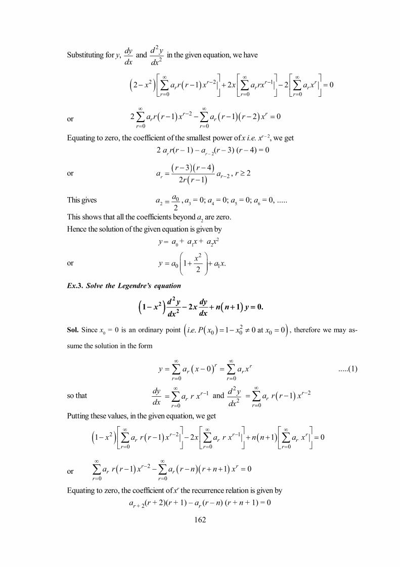
162
Substituting for y, dydx
and 2
2d ydx
in the given equation, we have
2 2 1
0 0 02 1 2 2 0r r r
r r rr r r
x a r r x x a rx a x
or 2
0 02 1 1 2 0r r
r rr r
a r r x a r r x
Equating to zero, the coefficient of the smallest power of x i.e. xr – 2, we get 2 ar r(r – 1) – ar – 2(r – 3) (r – 4) = 0
or ar
23 4
2 1 rr r
ar r
, r 2
This gives a20
2a
, a3 = 0; a4 = 0; a5 = 0; a6 = 0, .....
This shows that all the coefficients beyond a2 are zero.Hence the solution of the given equation is given by
y = a0 + a1x + a2x2
or y2
0 11 .2xa a x
Ex.3. Solve the Legendre’s equation
d y dyx x n n ydxdx
22
21 2 1 0.
Sol. Since x0 = 0 is an ordinary point 20 0 0. . 1 0 at 0i e P x x x , therefore we may as-
sume the solution in the form
y 0 0
0 r rr r
r ra x a x
.....(1)
so that dydx
1
0
rr
ra r x
and
2
2d ydx
2
01 r
rr
a r r x
Putting these values, in the given equation, we get
2 2 1
0 0 01 1 2 1 0r r r
r r rr r r
x a r r x x a r x n n a x
or 2
0 01 1 0r r
r rr r
a r r x a r n r n x
Equating to zero, the coefficient of xr the recurrence relation is given byar + 2(r + 2)(r + 1) – ar (r – n) (r + n + 1) = 0
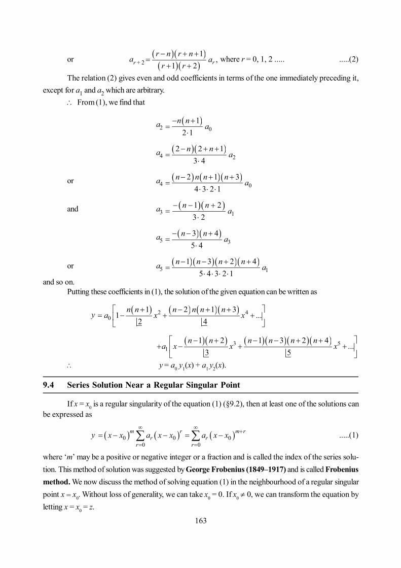
163
or ar + 2
1,
1 2 rr n r n
ar r
where r = 0, 1, 2 ..... .....(2)
The relation (2) gives even and odd coefficients in terms of the one immediately preceding it,except for a1 and a2 which are arbitrary.
From (1), we find that
a2
01
2 1n n
a
a4
22 2 1
3 4n n
a
or a4
02 1 3
4 3 2 1n n n n
a
and a3
11 23 2
n na
a5
33 45 4
n na
or a5
11 3 2 4
5 4 3 2 1n n n n
a
and so on.Putting these coefficients in (1), the solution of the given equation can be written as
y 2 4
01 2 1 3
1 ...2 4
n n n n n na x x
3 51
1 2 1 3 2 4...
3 5n n n n n n
a x x x
y = a0 y1(x) + a1 y2(x).
9.4 Series Solution Near a Regular Singular Point
If x = x0 is a regular singularity of the equation (1) (§9.2), then at least one of the solutions canbe expressed as
y 0 0 00 0
m r m rr r
r rx x a x x a x x
.....(1)
where ‘m’ may be a positive or negative integer or a fraction and is called the index of the series solu-tion. This method of solution was suggested by George Frobenius (1849–1917) and is called Frobeniusmethod. We now discuss the method of solving equation (1) in the neighbourhood of a regular singularpoint x = x0. Without loss of generality, we can take x0 = 0. If x0 0, we can transform the equation byletting x = x0 = z.
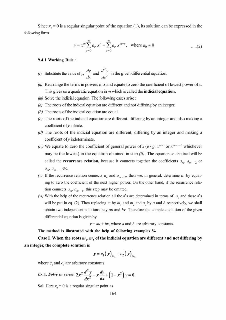
164
Since x0 = 0 is a regular singular point of the equation (1), its solution can be expressed in thefollowing form
00 0
, where 0m r m rr r
r ry x a x a x a
.....(2)
9.4.1 Working Rule :
(i) Substitute the value of y, dydx
and 2
2d ydx
in the given differential equation.
(ii) Rearrange the terms in powers of x and equate to zero the coefficient of lowest power of x.This gives us a quadratic equation in m which is called the indicial equation.
(iii) Solve the indicial equation. The following cases arise :(a) The roots of the indicial equation are different and not differing by an integer.(b) The roots of the indicial equation are equal.(c) The roots of the indicial equation are different, differing by an integer and also making a
coefficient of y infinite.(d) The roots of the indicial equation are different, differing by an integer and making a
coefficient of y indeterminate.(iv) We equate to zero the coefficient of general power of x (e g. xm + r or xm + r – 1 whichever
may be the lowest) in the equation obtained in step (ii). The equation so obtained will be
called the recurrence relation, because it connects together the coefficients am, am – 2 or
am, am – 1 etc.
(v) If the recurrence relation connects am and am – 2, then we, in general, determine a1 by equat-ing to zero the coefficient of the next higher power. On the other hand, if the recurrence rela-tion connects am, am – 1, this step may be omitted.
(vi) With the help of the recurrence relation all the as are determined in terms of a0 and these aswill be put in eq. (2). Then replacing m by m1 and m2 and a0 by a and b respectively, we shallobtain two independent solutions, say au and bv. Therefore the complete solution of the given
differential equation is given byy = au + bv, where a and b are arbitrary constants.
The method is illustrated with the help of following examples %
Case I. When the roots m1, m2 of the indicial equation are different and not differing byan integer, the complete solution is
1 2
1 2m my c y c y
where c1 and c2 are arbitrary constants
Ex.1. Solve in series d y dyx x x ydxdx
22 2
22 1 0.
Sol. Here x0 = 0 is a regular singular point as

165
0
lim 0x
Q xx
P x 1 20 0
1lim 0 lim 022x x
xx p x xx
finite
and
2
0lim 0x
R xx
P x
22 2
2 20 0
1 1lim 0 lim 022x x
xx p x xx
finite
therefore we assume the series solution in the form
y 00
, 0m rr
ra x a
.....(3)
Substituting for y, dydx
and 2
2d ydx
in the given equation, we find that
2 2 1 2
0 0 02 1 1 0m r m r m r
r r rr r r
x a m r m r x x a m r x x a x
or 2
0 01 2 2 1 0m r m r
r rr r
a m r m r x a x
.....(4)
which is an identity. Now equating to zero, the coefficient of smallest power x i.e. xm (put r = 0 in thefirst summation) then the equation (4) gives the indicial equation or quadratic equation in m as
a0(m – 1) (2m – 1) = 0which implies that m = 1, 1/2 as a0 0so the roots of the indicial equal are different and not differing by an integer.
To obtain the recurrence relation, we equate to zero the coefficient of xm + r and obtain
21
1 2 2 1r ra am r m r .....(5)
This formula connects ar with ar – 2. Now we proceed to find a1 as explained in step (v) of§ 9.4.1. For this purpose, we equate to zero, the coefficient of next higher power of x i.e. xm + 1
(put r = 1 in the first summation), we geta1[m(2m + 1)] = 0
Since the quantity within the bracket is not zero for any above values of m 11or ,2
this gives
a1 = 0Since a1 = 0, then from (5), we have a3 = a5 = ... = 0.Also taking r = 2, in (5), we get
a2 01
1 2 3a
m m
.....(6)
Next taking r = 4, in (5) and using (6), we obtain
a4 01
1 3 2 3 2 7a
m m m m
and so on.

166
Putting these values in (3), i.e. y = xm[a0 + a1x + a2x2 + a3x
3 + ...] gives
2 4
0 1 ...1 2 3 1 3 2 3 2 7
m x xy a xm m m m m m
.....(7)
Putting m = 1, and replacing a0 by a in (7), we get
y 2 41 11 ...2 5 2 4 5 9
ax x x au (say)
Next putting m = 1/2, and replacing a0 by b, we obtain
y2 4
1 2 1 ...2 3 2 3 4 7
x xbx bv (say)
Therefore the complete solution is given byy = au + bv,
where a and b are arbitrary constants.Ex.2. Solve the Gauss hypergeometric equation
2
21 1 0d y dyx x x ydxdx
in series in the neighbourhood of the regular singular point (i) x = 0 (ii) x = 1 and (iii) x = .Sol. Given
2
21 1 0d y dyx x x ydxdx
.....(8)
Dividing by x(1 – x), we get
2
21
01 1
xd y dy yx x dx x xdx
Comparing it with y + p1(x) y + p2(x) y = 0, we have
p1(x)
11
xx x
and p2(x) 1x x
Since x p1(x) and x2 p2(x) both tends to a finite value at x = 0, so x = 0 is regular singular pointof (8).
Case I. Solution in the neighbourhood of x = 0.We assume that the given equation (8) has the solution of the form
y 00
, 0m rr
ra x a
.....(9)
Substituting the values of y, yand yin the given equation (8), we get
2 2
01 m r
rr
x x a m r m r x

167
1
01 0m r m r
r rr
x a m r x a x
or 1
0 01 0m r m r
r rr r
a m r m r x a m r m r x
....(10)
which is an identity. Equating to zero, the coefficient of the smallest power of x i.e. xm – 1 (putr = 0 in the first summation), we get the indicial equation as
a0m(m – 1 + ) = 0, a0 0This gives m = 0, 1 – To obtain the recurrence relation, we equate to zero the coefficient of x m + r – 1. Then we have
ar(m + r) (m + r –1 + ) – ar –1(m + r –1 + ) (m + r –1 + ) = 0
or ar
11 1
1 rm r m r
am r m r
.....(11)
For the solution corresponding to m = 0, the recurrence relation (11) reduces to
ar
11 1
1 rr r
ar r
from which it follows that
a1 01a
,
a2
1 0
1 1 1 12 1 1 2 1
a a
and so on.Putting these values and m = 0 and replacing a0 by a in (2) gives
y
21 11 ....
1 1 2 1a x x
.....(12)
If we take a = 1 in (12), the series on the right hand side of (12) is called the hypergeometricseries and is represented by 2F1 (, , ; x). Thus we see that 2F1 (, , ; x) is a solution of (8).
For the solution corresponding to m = 1 – , when 1 – is neither zero nor an integer, therecurrence relation (11) reduces to.
ar
11 1 1 1
1 1 1 rr r
ar r
or ar
1
1 11 r
r ra
r r
.....(13)
where = 1 – +, = 1 – + , = 2 – .....(14)Replacing r = 1, 2, 3, .... successively in (13), we have
a1 01a
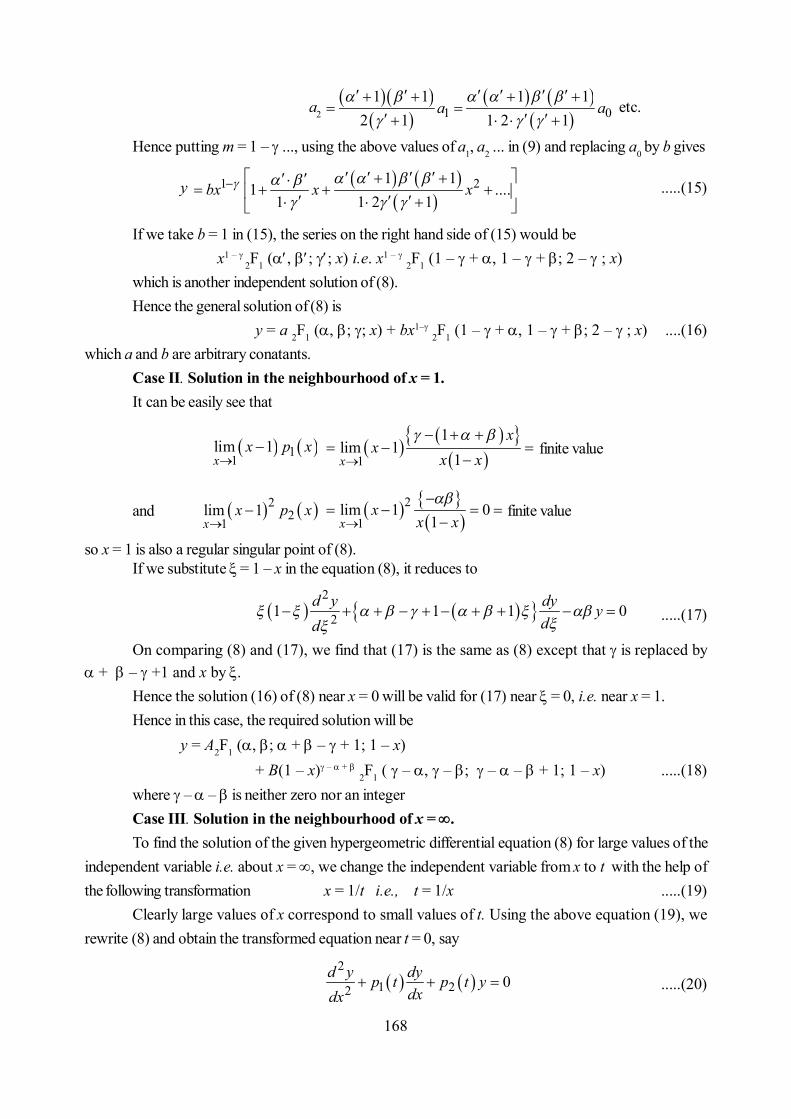
168
a2
1 01 1 1 1
2 1 1 2 1a a
etc.
Hence putting m = 1 – ..., using the above values of a1, a2 ... in (9) and replacing a0 by b gives
y
1 21 11 ....
1 1 2 1bx x x
.....(15)
If we take b = 1 in (15), the series on the right hand side of (15) would bex1 –
2F1 (, ; ; x) i.e. x1 – 2F1 (1 – + ,1 – +; 2 – ; x)which is another independent solution of (8).Hence the general solution of (8) is
y = a 2F1 (, ; ; x) + bx1– 2F1 (1 – + ,1 – +; 2 – ; x) ....(16)which a and b are arbitrary conatants.
Case II. Solution in the neighbourhood of x = 1.It can be easily see that
11
lim 1x
x p x
1
1lim 1
1x
xx
x x
finite value
and 22
1lim 1x
x p x
21
lim 1 01x
xx x
finite value
so x = 1 is also a regular singular point of (8).If we substitute = 1 – x in the equation (8), it reduces to
2
21 1 1 0d y dy ydd
.....(17)
On comparing (8) and (17), we find that (17) is the same as (8) except that is replaced by+ – +1 and x by .
Hence the solution (16) of (8) near x = 0 will be valid for (17) near = 0, i.e. near x = 1.Hence in this case, the required solution will be
y = A2F1 (, ; + – + 1; 1 – x)+ B(1 – x)– + 2F1 ( – , –; – – + 1; 1 – x) .....(18)
where –– is neither zero nor an integerCase III. Solution in the neighbourhood of x = .To find the solution of the given hypergeometric differential equation (8) for large values of the
independent variable i.e. about x = , we change the independent variable from x to t with the help ofthe following transformation x = 1/t i.e., t = 1/x .....(19)
Clearly large values of x correspond to small values of t. Using the above equation (19), werewrite (8) and obtain the transformed equation near t = 0, say
2
1 22 0d y dyp t p t ydxdx
.....(20)

169
Then the given equation (8) is said to have a regular singular point at x = if the transformedequation (20) has regular singular point at t = 0.
For x 21 1 1or , dttt x dx x
.....(21)
and y 221
dy dy dt dy dytdx dt dx dt dtx
.....(22)
Also y2 2
4 32 2 2
d y d dy d dy dt d y dyt tdx dx dt dx dx dtdx dt
.....(23)
Using (21), (22) and (23), the given equation (8) transforms to
2
221 2 1 1 0d y dyt t t t t y
dtdt .....(24)
To solve (24), let its series solution be
y 00
, 0m rr
ra t a
.....(25)
so that 1
0
m rr
r
dy a m r tdt
and
22
20
1
m r
rr
d y a m r m r tdt
Putting these values of y, dydt
and 2
2d ydt
in (24), we get
3 2 2
0
1
0 0
1
2 1 1 0
m rr
r
m r m rr r
r r
t t a m r m r t
t t t a m r t a t
or 1
0 01 0
m r m r
r rr r
a m r m r t a m r m r t .....(26)
which is an identity. Equating to zero, the coefficient of the smallest power of t (put r = 0, in the firstsummation), we get
a0(m –) (m – ) = 0 m = , as a0 0Next equating to zero, the coefficient of tm + r + 1 in (26), we find that
ar + 1
1
1 1 rm r m r
am r m r
.....(27)
For the solution, corresponding to m = , the recurrence relation (27) reduces to
ar + 1
11 1 rr r
ar r
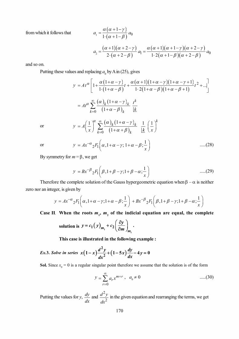
170
from which it follows that a1
0
11 1
a
a2
1 0
1 2 1 1 22 2 1 2 1 2
a a
and so on.Putting these values and replacing a0 by A in (25), gives
y
21 1 1 1 11 ...
1 1 1 2 1 1 1At t t
0
11
kk k
k k
tAtk
or y 0
11 1 11
kk k
k kA
x k x
or y 2 11,1 ; 1 ;
Ax F
x .....(28)
By symmetry for m = , we get
y 2 11,1 ;1 ;Bx Fx
.....(29)
Therefore the complete solution of the Gauss hypergeometric equation when – is neitherzero nor an integer, is given by
y 2 11,1 ;1 ;Ax Fx
2 11,1 ;1 ;Bx Fx
Case II. When the roots m1, m2 of the indicial equation are equal, the complete
solution is mm
yy c y cm1
1
1 2 .
This case is illustrated in the following example :
Ex.3. Solve in series 2
21 1 5 4 0d y dyx x x ydxdx
Sol. Since x0 = 0 is a regular singular point therefore we assume that the solution is of the form
y0
m rr
ra x
, a0 0 .....(30)
Putting the values for y, dydx
and 2
2d ydx
in the given equation and rearranging the terms, we get

171
2 21
0 02 0m r m r
r rr r
a m r x a m r x
.....(31)
Equating to zero, the coefficients of lowest power of x, the indicial equation givesa0m
2= 0m = 0, 0 as a0 0.Since both the values of m are equal so it gives us only one independent solution. Equating to
zero, the coefficient of xm + r, we find that
ar + 1
221
r
m r am r
.....(32)
Which gives a1 0
221
m am
a2 1
2 2
03 32 1
m ma am m
and so on.Hence the solution is given by
y 2 2 2
2 30
2 3 41 ...1 1 1
m m m ma x x x xm m m
.....(33)
Putting m = 0 and replacing a0 by a in (33) givesy = a [1 + 22x + 32x2 + 42x3 + ...] = au (say) .....(34)
To get the second solution, we procecd as follows :Rewriting (33)
2 21 2
02 3 ....1 1
m m mm my a x x xm m
which on differentiation with respect to x gives
2 2
1 10
2 31 2 ....1 1
m m mdy m ma mx m x m xdx m m
and
2 22
2 102
2 31 1 2 1 ....1 1
m m md y m ma m m x m mx m m xm mdx
Putting the values of y, dydx
and 2
2d ydx
in the left hand side of the given equation, we get
2 2
2 2 10
2 31 1 1 2 ...1 1
m m mm mx x a m m x m m x m m xm m

172
2 2
1 10
2 31 5 1 2 ...1 1
m m mm mx a mx m x m xm m
2 21 2 2 1
0 02 34 ...1 1
m m m mm ma x x x a m xm m
The coefficient of remaining powers of x being zero, it can be easily verified by considering thecoefficients one by one.
Thus we may write
2
2 2 102 1 5 4 md y dyx x x y a m x
dxdx
which on partial differentiation with respect to m, gives
2
2 1 2 10 02 1 5 4 2 logm md dx x x y a mx a m x x
m dxdx
Since the operators are commutative, therefore the above relation may be rewritten as
2
2 1 2 10 02 1 5 4 2 logm md d yx x x a mx a m x x
dx mdx
Putting m = 0, we get
2
22
01 5 4
m
d d yx x xdx mdx
which shows that 0m
ym
is a second solution of the given differential equation.
Hence differentiating (33) partially with respect to m, we get
2 22
02 3log 1 ...1 1
my m ma x x x xm m m
0 222 12 ...
1 1 1m mma x x
m m m
22
33 12 ...1 1 1
mm xm m m
Putting m = 0 and replacing a0 by b gives
0m
ym
2 2 2log 1 2 3 ...b x x x 22 2 1 2 3 1 3 .... b x x
0m
ym
2log 2 1 2 2 3 ... ,b u x x x bv (say)

173
Thus the required solution isy = au + bv,
where a and b are arbitrary constants.Case III. When the roots m1, m2 (m1 > m2) of the indicial equation are different and
differing by an integer and also making a coefficient of y infinite.Working Rule. If the indicial equation has unequal roots, say m1 and m2 (m1 > m2) differing by
an integer and if some of the coefficients of y become infinite when m = m2, we modify the form of y byreplacing a0 by d0(m – m2) where d0 0. Then two independent solutions can be obtained by putting
m = m2 in the modified form of y and ym
. In this case the solution by putting m = m1 in y is rejected
because it only gives a numerical multiple of the solution obtained by putting m = m2 in modified y. Thusthe complete solution is
y 2
2
1 2mm
yc y cm
Ex.4. Solve 2
2 22 1 0d y dyx x x y
dxdx in series.
Sol. Given 2
2 22 1 0d y dyx x x y
dxdx .....(35)
Since x = 0 is a regular singular point as x p1(x) and x2 p2(x) tends to a finite limit as x 0,therefore we assume the solution of the given equation (35) in the form
y 00
, 0m rr
ra x a
then 1 2
0 0, 1m r m r
r rr r
y a m r x y a m r m r x
Substituting for y, y and y in (35), then it gives
2 2 1 2
0 0 01 1 0m r m r m r
r r rr r r
x a m r m r x x a m r x x a x
or 2
0 01 1 0m r m r
r rr r
a m r m r m r x a x
or 2
0 01 1 0m r m r
r rr r
a m r m r x a x
.....(36)
which is an identity. Equating to zero, the coefficients of the smallest power of x, namely xm (put r = 0 inthe first summation), gives the indicial equation
a0(m + 1) (m – 1) = 0so that m= 1, – 1 as a0 0 .....(37)
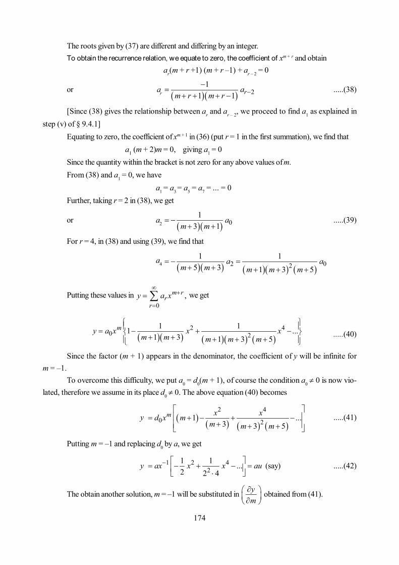
174
The roots given by (37) are different and differing by an integer.To obtain the recurrence relation, we equate to zero, the coefficient of xm + r and obtain
ar(m + r +1) (m + r –1) + ar – 2 = 0
or ar 21
1 1 ram r m r
.....(38)
[Since (38) gives the relationship between ar and ar – 2, we proceed to find a1 as explained instep (v) of § 9.4.1]
Equating to zero, the coefficient of xm + 1 in (36) (put r = 1 in the first summation), we find thata1(m + 2)m = 0, giving a1 = 0
Since the quantity within the bracket is not zero for any above values of m.From (38) and a1 = 0, we have
a1 = a3 = a5 = a7 = ... = 0Further, taking r = 2 in (38), we get
or a2 01
3 1a
m m
.....(39)
For r = 4, in (38) and using (39), we find that
a4 2 02
1 15 3 1 3 5
a am m m m m
Putting these values in 0
,m rr
ry a x
we get
2 4
0 21 11 ...
1 3 1 3 5my a x x x
m m m m m
.....(40)
Since the factor (m + 1) appears in the denominator, the coefficient of y will be infinite form = –1.
To overcome this difficulty, we put a0 = d0(m + 1), of course the condition a0 0 is now vio-lated, therefore we assume in its place d0 0. The above equation (40) becomes
y
2 40 21 ...
3 3 5m x xd x m
m m m
.....(41)
Putting m = –1 and replacing d0 by a, we get
y 1 2 42
1 1 ...2 2 4
ax x x au
(say) .....(42)
The obtain another solution, m = –1 will be substituted in ym
obtained from (41).

175
Nowym
2 40 2log 1 ...
3 3 5m x xd x x m
m m m
24
0 2 3 2 22 11 ...
3 3 5 3 5m xd x x
m m m m m
Putting m = –1, replacing d0 by b, the second solution will be obtained as
1m
ym
1 2 42
1 1log ...2 2 4
bx x x x
1 2 4
2 21 1 2 11 ...
2 42 2 4bx x x
21 4
2 2 25log 1 ...
2 2 4
xbu x bx x
21 4
2 2 25log 1 ...
2 2 4xb u x x x
.....(43)
= b v (say)
Hence the complete solution of the given differential equation is
y = au + bv.
Note : If we substitute m = 1 and 012
d in (41), we get
y4
22
11 ...2 4 2 4 6
xx x
y3 5
2 . 22 4 2 4 6x xx u
which gives no new independent solution.
Case IV. When the roots m1, m2 of the indicial equation are different and differing by
an integer and also making a coefficient of y indeterminate.
Working Rule. If the indicial equation has two different roots say m1, m2 (m1 > m2) differing by
an integer and if one of the coefficients of y become indeterminate when m = m2, the complete solution
is given by putting m = m2 in y, which contains two arbitrary constants. In this case, the solution obtained
by putting m = m1 in y is rejected because it only gives a numerical multiple of one of the series con-
tained in the first solution.

176
Ex.5. Solve d y dyx x x x ydxdx
22 2
2 9 0 in series.
Sol. Since x0 = 0 is a regular singular point, we assume the solution in the form
y0
m rr
ra x
, a0 0
then 2 2 2 1
0 01 m r m r
r rr r
x a m r m r x x x a m r x
0
9 0m rr
rx a x
or 1
0 01 9 1 0m r m r
r rr r
a m r m r m r x a m r x
or 1
0 03 3 1 0m r m r
r rr r
a m r m r x a m r x
which is an identity. Equating to zero, the coefficient of the smallest power of x, namely xm
(putting r = 0 in the first summation), we geta0(m – 3) (m + 3) = 0, m = 3, –3 ( a0 0)
The roots of the equation are different and differing by an integer. To obtain the recurrence rela-tion, we equate to zero, the coefficient of the general term i.e. xm + r, we get
ar(m + r + 3) (m + r – 3) + ar – 1(m + r) = 0
or ar
13 3 r
m ra
m r m r
.....(44)
Taking m = –3, we get ar
1
36 r
ra
r r
Thus for r = 1, we have a1 02
5a
and for r = 2, 3, 4, 5, and 6 we have
a2 1 01 2 18 5 8
a a
a3 = 0, a4 = 0, a5 = 0 and
a6
56 3 0
6 6 6 0a
(inderminate)
and may be taken as a free constant
Also a7 6 8 7 64 5 4 5and
7 16 7 16a a a a
and so on.

177
y 2 30 1 2 3
0...m r m
rr
a x x a a x a x a x
y 3 2 6 7 80 1 2 6 7 8 ...x a a x a x a x a x a x
3 20 0 0
2 1 25 8 5
x a a x a x 3 6 7 8
6 6 64 4 5 ...7 7 16
x a x a x a x
y 3 2 3 20 6
2 2 1 4 4 51 1 ...5 5 8 7 7 16
a x x x a x x x
This contains two arbitrary constants a0 and a6 and therefore may be taken as the complete so-lution
Note. If we put m = 3 in (44), we get a series solution
y 3 20
4 4 51 ...7 7 16
a x x x which gives no new independent solution.
9.5 Series Solution in Descending Powers of the Independent Variable
Till now we have obtained series solutions in ascending powers of the independent variable. How-ever, the following cases may arise.
(i) There exists no solution of the form 0
m rr
ra x
.
(ii) The usual Frobenius method breaks down.(iii) The series solution obtained by earlier methods does not converge.In such cases we obtain the series solution in descending powers of the independent variable.
Sometimes, the series solution in descending powers are desirable and are more useful in practice.Working Rule
(i) We assume a solution of the form 00
, 0m rr
ry a x a
(ii) For indicial equation, we equate to zero the coefficient of the highest power of x in the iden-tity.
(iii) For recurrence relation, the coefficient of the higher power, in general, in the identity is equatedto zero.
To illustrate the method we consider following examples :Ex.1. Integrate in descending series the Legendre’s equation or determine the solution of
Legendre’s equation.Sol. The differential equation of the form
(1 – x2) y– 2x y + n(n + 1) y = 0 .....(1)

178
is called the Legendre’s equation, where n N. Let the series solution of (1) be of the form
y 00
, 0m rr
ra x a
.....(2)
Substituting the values of y, y and y in the given equation, we get
2 2 1
0 0 01 1 2 1 0m r m r m r
r r rr r r
x a m r m r x x a m r x n n a x
or 2
0 01 1 0m r m r
r rr r
a m r m r x a m r n m r n x
.....(3)
which is an identity. Equating to zero, the coefficient of the highest power of x, namely xm, (putr = 0 in the second summation), we get the indicial equation
a0(m – n) (m + n + 1) = 0Since a0 0 m = n, – (n + 1)
which shows that the roots are different.To obtain the recurrence relation, we equate to zero the coefficient of xm – r and obtain
ar –2(m – r + 2) (m – r + 1) – ar(m – r – n) (m – r + n + 1) = 0
or ar
22 1
1 rm r m r
am r n m r n
.....(4)
Here we need to evaluate a1. It can be done by equating to zero, the coefficient of the nextlower power of x i.e. xm – 1, which gives
a1(m – 1 – n) (m + n) = 0 a1 = 0, since the quantity within the bracket is not zero for any above values of mSince a1 = 0, then from (4), we have a3 = a5 = .... = 0
Also a2
01
2 1m m
am n m n
a4
22 14 3
m ma
m n m n
a4
01 2 3
2 4 1 3m m m m
am n m n m n m n
Putting these values in (2), the solution is.
2 4
01 1 2 3
1 ...2 1 2 4 1 3
m m m x m m m m xy a x
m n m n m n m n m n m n
.....(5)
When m = n, replacing a0 by a, in (5) one of the solution is
2 41 1 2 31 ...
2 2 1 2 4 2 1 2 3n n n n n n n
y ax x x aun n n
(say) .....(6)
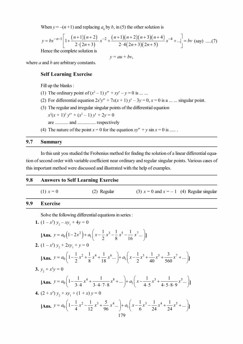
179
When y = –(n +1) and replacing a0 by b, in (5) the other solution is
1 2 41 2 1 2 3 41 ...
2 2 3 2 4 2 3 2 5n n n n n n n
y bx x x bvn n n
(say) .....(7)
Hence the complete solution isy = au + bv,
where a and b are arbitrary constants.
Self Learning Exercise
Fill up the blanks :(1) The ordinary point of (x2 – 1) y + xy – y = 0 is ... ...(2) For differential equation 2x2y + 7x(x + 1) y – 3y = 0, x = 0 is a ... ... singular point.(3) The regular and irregular singular points of the differential equation
x2(x + 1)2 y + (x2 – 1) y + 2y = 0are ........... and ............... respectively
(4) The nature of the point x = 0 for the equation xy + y sin x = 0 is ..... .
9.7 Summary
In this unit you studied the Frobenius method for finding the solution of a linear differential equa-tion of second order with variable coefficient near ordinary and regular singular points. Various cases ofthis important method were discussed and illustrated with the help of examples.
9.8 Answers to Self Learning Exercise
(1) x = 0 (2) Regular (3) x = 0 and x = – 1 (4) Regular singular
9.9 Exercise
Solve the following differential equations in series :1. (1 – x2) y2 – xy1 + 4y = 0
[Ans. 2 3 5 70 1
1 1 11 2 ...2 8 16
y a x a x x x x ]
2. (1 – x2) y2 + 2xy1 + y = 0
[Ans. 2 4 6 3 5 70 1
1 1 1 1 1 31 ... ...2 8 18 2 40 560
y a x x x a x x x x
]
3. y2 + x2y = 0
[Ans. 4 8 3 50 1
1 1 1 11 ... ...3 4 3 4 7 8 4 5 4 5 8 9
y a x x a x x x ]
4. (2 + x2) y2 + xy1 + (1 + x) y = 0
[Ans. 2 3 4 3 4 50 1
1 1 5 1 1 11 ... ...4 12 96 6 24 24
y a x x x a x x x x
]
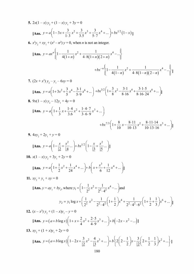
180
5. 2x(1 – x) y2 + (1 – x) y1 + 3y = 0
[Ans. 2 3 4 1 23 3 31 3 ... 11 3 3.5 5 7
y a x x x x bx x ]
6. x2y2 + xy1 + (x2 – n2) y = 0, when n is not an integer.
[Ans. 2 41 11 ...
4 1 4 8 1 2ny ax x x
n n n
2 41 11 ...
4 1 4 8 1 2nbx x x
n n n
]
7. (2x + x3) y2 – y1 – 6xy = 0
[Ans. 2 4 63 3 11 3 ...5 5 9
y a x x x 3 2 2 4 63 3 1 3 1 51 ...
8 8 16 8 16 24bx x x x
]
8. 9x(1 – x) y2 – 12y1 + 4y = 0
[Ans. 2 31 1 4 1 4 71 ...3 3.6 3 6 9
y a x x x
7 3 2 38 8 11 8 11 141 ...10 10 13 10 13 16
bx x x x ]
9. 4xy2 + 2y1 + y = 0
[Ans. 2 2
1 21 ... 1 ...2 4 3 5x x x xy a bx
]
10. x(1 – x) y2 + 3y1 + 2y = 0
[Ans. 3
2 4 41 1 11 ... ...2 24 6 12
xy a x x b x x
]
11. xy2 + y1 + xy = 0
[Ans. y = ay1 + by2, where 2 41 2 2 2
1 11 ...2 2 4
y x x and
2 4 62 1 2 2 2 2 2 2
1 1 1 1 1 1log 1 1 ...2 2 32 2 4 2 4 6
y y x x x x ]
12. (x – x2) y2 + (1 – x)y1 – y = 0
[Ans. 2 3 22 2 5log 1 ... 2 ...4 4 9
y a b x x x x b x x ]
13. xy2 + (1 + x)y1 + 2y = 0
[Ans. 2 3 23 4 1 3 1 1log 1 2 ... 2 2 2 ...2 3 2 2 2 3
y a b x x x x b x x
]

181
14. x(1 – x2) y2 + (1 – 3x2)y1 – xy = 0
[Ans. 2 2 2
2 4 42 2 2
1 1 3 1 21log 1 ... ...4 1282 2 4
y a b x x x b x x
]
15. x(1 – x) y2 – (1 + 3x)y1 – y = 0
[Ans. 2 3 2log 1 2 2 3 ... 1 5 ...y a b x x x b x x ]
16. xy2 + xy1 + (x2 – 4)y = 0
[Ans. 2 4 6 82 3 3 21 1 1log ...
2 4 2 4 6 2 4 6 8y a b x x x x x
2 2 4 62 2 2 2 2 2
1 1 11 ...2 2 4 2 4 6
bx x x x ]
17. x(1 – x) y2 – 3xy1 – y = 0
[Ans. 2 3 2log 2 3 ... 1 ...y a b x x x x b x x ]
18. x2y2 + x(1 + 2x)y1 – 4y = 0
[Ans. 2 2 2 20 4
4 2 4 41 1 ...3 3 5 10
y a x x x a x x x
]
19. (1 – x2)y2 + 2xy1 + y = 0
[Ans. 3
2 4 50 1
1 1 11 ... ...2 8 2 40
xy a x x a x x
]

182
Unit 10 : Gauss Hypergeometric Function: its Properties AndIntegral Representation
Structure of the Unit
10.0 Objective
10.1 Introduction
10.2 Convergence of the Series
10.3 Special Cases of the Gauss Function
10.4 Integral Representation
10.4.1 Deductions
10.5 Gauss Hypergeometric Differential Equation and Its Solution
10.6 Two Summation Theorems
10.6.1 Theorem 1
10.6.2 Theorem 2
10.7 Summary
10.8 Answers of Self -Learning Exercise
10.9 Exercise
10.0 Objective
The aim of this unit is to study a special function known as Gauss hypergeometric function. Alsoits special cases, properties, convergence conditions and summation theorems such as Gauss’s theorem,Kummer’s theorem and Vandermonde’s theorem are obtained.
10.1 Introduction
The series
2 31 1 1 2 1 21 ...
1 2 1 2 3a a b b a a a b b bab z zz
c c c c c c
.....(1)
is called the Gauss series or the Ordinary hypergeometric series. It is usually represented by the symbol
2F1 (a, b ; c ; z), The three quantities a, b and c are called the parameters and z is the variable of theseries. All these four quantities may be any number, real or complex. In the notation 2F1 (.), the left suffix
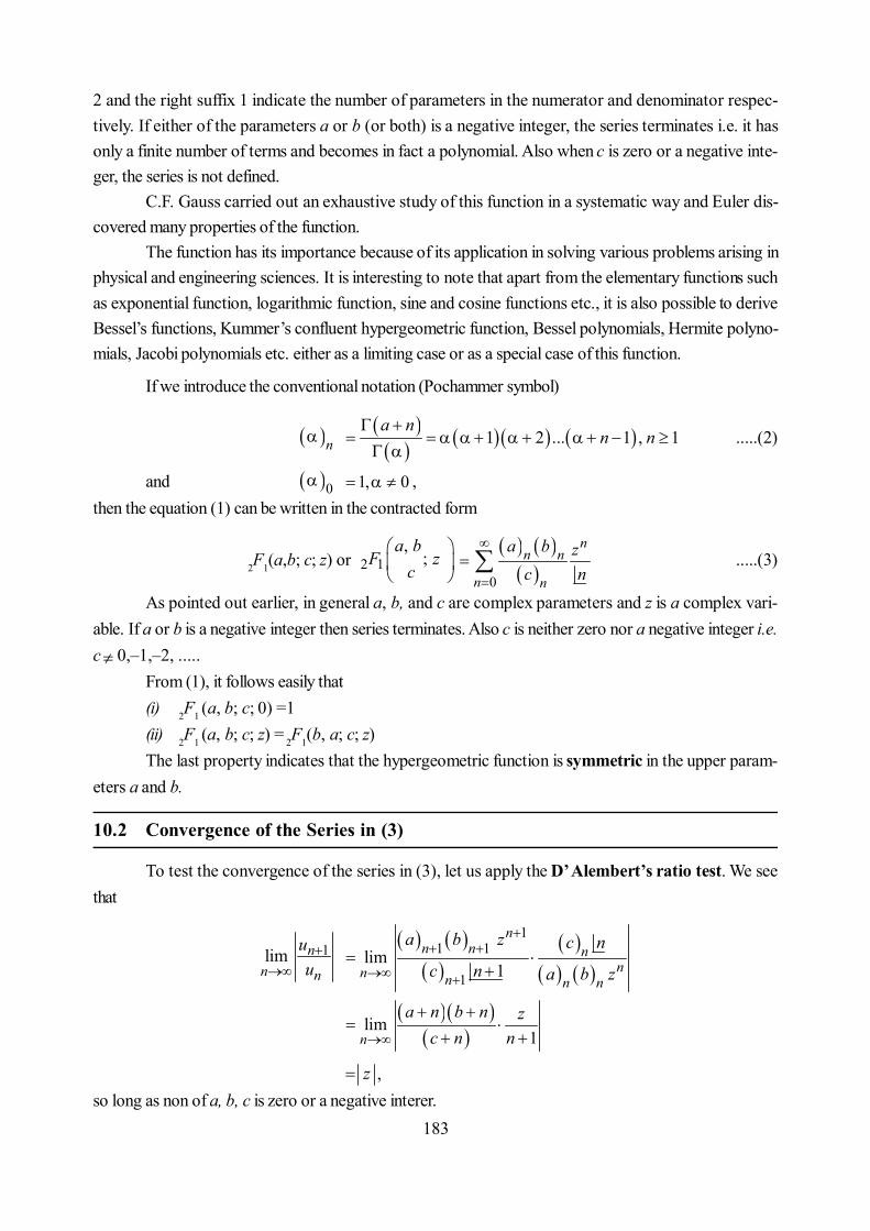
183
2 and the right suffix 1 indicate the number of parameters in the numerator and denominator respec-tively. If either of the parameters a or b (or both) is a negative integer, the series terminates i.e. it hasonly a finite number of terms and becomes in fact a polynomial. Also when c is zero or a negative inte-ger, the series is not defined.
C.F. Gauss carried out an exhaustive study of this function in a systematic way and Euler dis-covered many properties of the function.
The function has its importance because of its application in solving various problems arising inphysical and engineering sciences. It is interesting to note that apart from the elementary functions suchas exponential function, logarithmic function, sine and cosine functions etc., it is also possible to deriveBessel’s functions, Kummer’s confluent hypergeometric function, Bessel polynomials, Hermite polyno-mials, Jacobi polynomials etc. either as a limiting case or as a special case of this function.
If we introduce the conventional notation (Pochammer symbol)
n 1 2 ... 1 , 1a n
n n
.....(2)
and 0 1, 0 ,then the equation (1) can be written in the contracted form
2F1(a,b; c; z) or 2 1,
;a b
F zc
0
nn n
n n
a b zc n
.....(3)
As pointed out earlier, in general a, b, and c are complex parameters and z is a complex vari-able. If a or b is a negative integer then series terminates. Also c is neither zero nor a negative integer i.e.c 0,–1,–2, .....
From (1), it follows easily that(i) 2F1 (a, b; c; 0) =1(ii) 2F1 (a, b; c; z) = 2F1(b, a; c; z)The last property indicates that the hypergeometric function is symmetric in the upper param-
eters a and b.
10.2 Convergence of the Series in (3)
To test the convergence of the series in (3), let us apply the D’ Alembert’s ratio test. We seethat
1lim nn n
uu
11 1
1lim
1
nn n n
nn n n n
a b z c nc n a b z
lim1n
a n b n zc n n
z ,so long as non of a, b, c is zero or a negative interer.
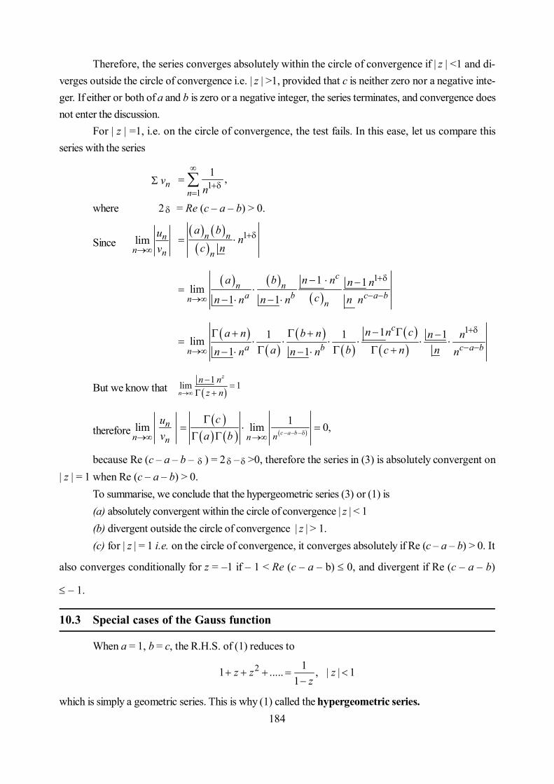
184
Therefore, the series converges absolutely within the circle of convergence if | z | <1 and di-verges outside the circle of convergence i.e. | z | >1, provided that c is neither zero nor a negative inte-ger. If either or both of a and b is zero or a negative integer, the series terminates, and convergence doesnot enter the discussion.
For | z | =1, i.e. on the circle of convergence, the test fails. In this ease, let us compare thisseries with the series
nv 11
1 ,n n
where 2 = Re (c – a – b) > 0.
Since lim nn n
uv
1n n
n
a bn
c n
11 1lim1 1
cn n
a b c a bn n
a b n n n ncn n n n n n
111 1 1lim1 1
c
a b c a bn
n n ca n b n n na b c n nn n n n n
But we know that 1lim 1
z
n
n nz n
therefore lim nn n
uv
1lim 0,c a bnn
ca b
because Re (c – a – b – ) = 2 – >0, therefore the series in (3) is absolutely convergent on| z | = 1 when Re (c – a – b) > 0.
To summarise, we conclude that the hypergeometric series (3) or (1) is(a) absolutely convergent within the circle of convergence | z | < 1(b) divergent outside the circle of convergence | z | > 1.(c) for | z | = 1 i.e. on the circle of convergence, it converges absolutely if Re (c – a – b) > 0. It
also converges conditionally for z = –1 if – 1 < Re (c – a – b) 0, and divergent if Re (c – a – b)
– 1.
10.3 Special cases of the Gauss function
When a = 1, b = c, the R.H.S. of (1) reduces to
2 11 ..... , | | 11
z z zz
which is simply a geometric series. This is why (1) called the hypergeometric series.
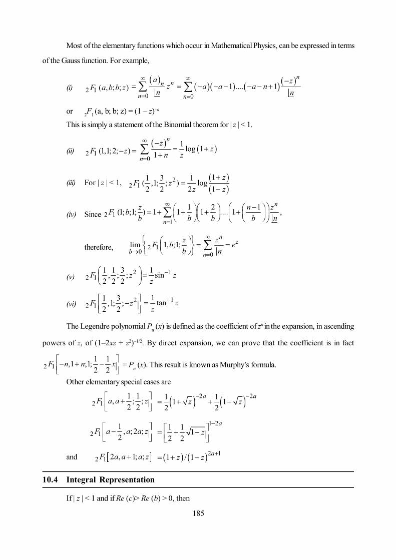
185
Most of the elementary functions which occur in Mathematical Physics, can be expressed in terms
of the Gauss function. For example,
(i) 2 1 ( , ; ; )F a b b z
0
nn
n
az
n
01 .... 1
n
n
za a a n
n
or 2F1 (a, b; b; z) = (1 – z)–a
This is simply a statement of the Binomial theorem for | z | < 1.
(ii) 2 1 (1,1;2; )F z
0
1 log 11
n
n
zz
n z
(iii) For | z | < 1,
22 1
11 3 1( ,1; ; ) log2 2 2 1
zF z
z z
(iv) Since 2 11
1 2 1(1; ;1; ) 1 1 1 .... 1 ,n
n
z n zF bb b b b n
therefore, 2 10 0
lim 1, ;1;n
zb n
z zF b eb n
(v) 2 12 1
1 1 3 1, ; ; sin2 2 2
F z zz
(vi) 22 1
1 3,1; ;2 2
F z 11 tan z
z
The Legendre polynomial Pn (x) is defined as the coefficient of zn in the expansion, in ascending
powers of z, of (1–2xz + z2)–1/2. By direct expansion, we can prove that the coefficient is in fact
2 11 1,1 ;1;2 2
F n n x = Pn (x). This result is known as Murphy’s formula.
Other elementary special cases are
2 11 1, ; ;2 2
F a a z 2 21 11 1
2 2a a
z z
2 11 , ;2 ;2
F a a a z
1 21 1 12 2
az
and 2 1 2 , 1; ;F a a a z 2 11 / 1 az z
10.4 Integral Representation
If | z | < 1 and if Re (c)> Re (b) > 0, then

186
B (b, c – b) 2F1 (a, b ; c ; z) 1
11
0
1 1c b abt t zt dt
or 2F1 (a,b;c;z)
1
11
0
1 1c b abct t zt dt
b c b
.....(1)
Proof. Let I 1
11
0
1 1c b abt t zt dt
111
00
1r
c bb r
r
a ztt t dt
r
Now interchanging the order of integration and summation, we see that
I
111
0 0
1r
c bb rr
r
a zt t dt
r
0
rr
r
a zb r c bc r r
0
rr r
r r
a bb zc bc c r
= B (b, c – b) 2F1 (a, b ; c ; z)
10.4.1 Deductions from integral representation
As a consequence of equation (1), we derive the Gauss’s theorem which gives rise to
Vandermonde’s theorem of the hypergeometric function. Kummer’s theorem is also derived. These
theorems are of great importance in the study of various special functions of mathematical physics.
(a) Gauss’s theorem. If Re (c – a – b) > 0, Re (c) > 0, then
F a,b;c;2 1 1 c c a bc a c b
Prof. Putting z = 1 in the equation (1), we get
2 1 , ; ;1F a b c
1
11
0
1 c a bbct t dt
b c b
=
c b c a b
b c b c a
2 1 , ; ;1F a b c = c c a bc a c b
.....(2)

187
(b) Vandermonde’s theorem
F n b c2 1 , ; ;1
n
n
c b=
c
Prof. If we make a = – n in eq. (2), where n is a positive integer, then we get
2 1 , ; ;1F n b c
n n
n
c c b n c bc n c b c
(c) Kummer’s Theorem
F a b a b 2 1 , ;1 ; 1
ba b
bb a
1 12
1 12
.....(3)
Prof. To prove (3), we put z – 1 and c = 1 – a + b in equation (1), we abtain
2 1 , ;1 ; 1F a b a b
11 2
0
11
1aba b
t t dtb a
fdgdg .....(4)
Putting t2 = u in the above equation (4), we get
2 1 , ;1 ; 1F a b a b
1
1 12 1
0
11
2 1aba b
u u dub a
11 22 1 1
2
b aa bbb a a
2 1 , ;1 ; 1F a b a b
1 / 2 11 1 / 2
b a bb a b
10.5 Gauss’s Hypergeometric Differential Equation and its Solution
Let = .dzdz Then zn = nzn
Therefore, (+ c – 1) zn = n (n + c – 1) zn.
Now y = 2 1 , ; ;F a b c z 0
nn n
n n
a bz
c n
We have 1c y
0
1 nn n
n n
n n c a bz
c n
1 1
1nn n
n n
a bz
c n

188
11 1
0
nn n
n n
a bz
c n
0
nn n
n n
a n b n a bz
c n
= z (+ a) (+ b) y
0
since nn n
n n
a n a ba y z
c n
Hence y =2F1 (a ,b; c; z) is a solution of differential equation
1 0, dc z a b y zdz
The above equation can be easily written in the following form
d y dyz z c a b z ab ydz dz
2
21 1 0 .....(1)
(by employing the relations y = zy and ( – 1) y = z2y) is known as Gauss’s hypergeometricdifferential equation.
From the theory of differential equation, it follows that the regular singular points of the aboveequation (1) are:
(i) z = 0 with exponents 0, 1 – c(ii) z =1 with exponents 0, c – a – b(iii) z =with exponents a,b.For details of the solution of the differential equation (1), students are advised to reter Ex. 2 in
§9.4 of the last unit.
10.6 Two summation Theorems
In this section, we discuss two theorems concerning elementary series manipulations which areimportant techniques in establishing several transformation formulae, summation formulae and in investi-gating several other properties of hypergeometric functions, Bessel’s functions and Orthogonal polyno-mials etc.
10.6.1 Theorem 1.
m n
n m
0 0,
m
m nn m n
0 0
, .....(1)
and. m
m nn m
0 0,
m nn m n
0 0
, .....(2)
Proof. Consider the L.H.S. of the equation (1) in which the term um + n has been inserted forconvenience i.e.
0 0
, m n
m nn m u
.....(3)
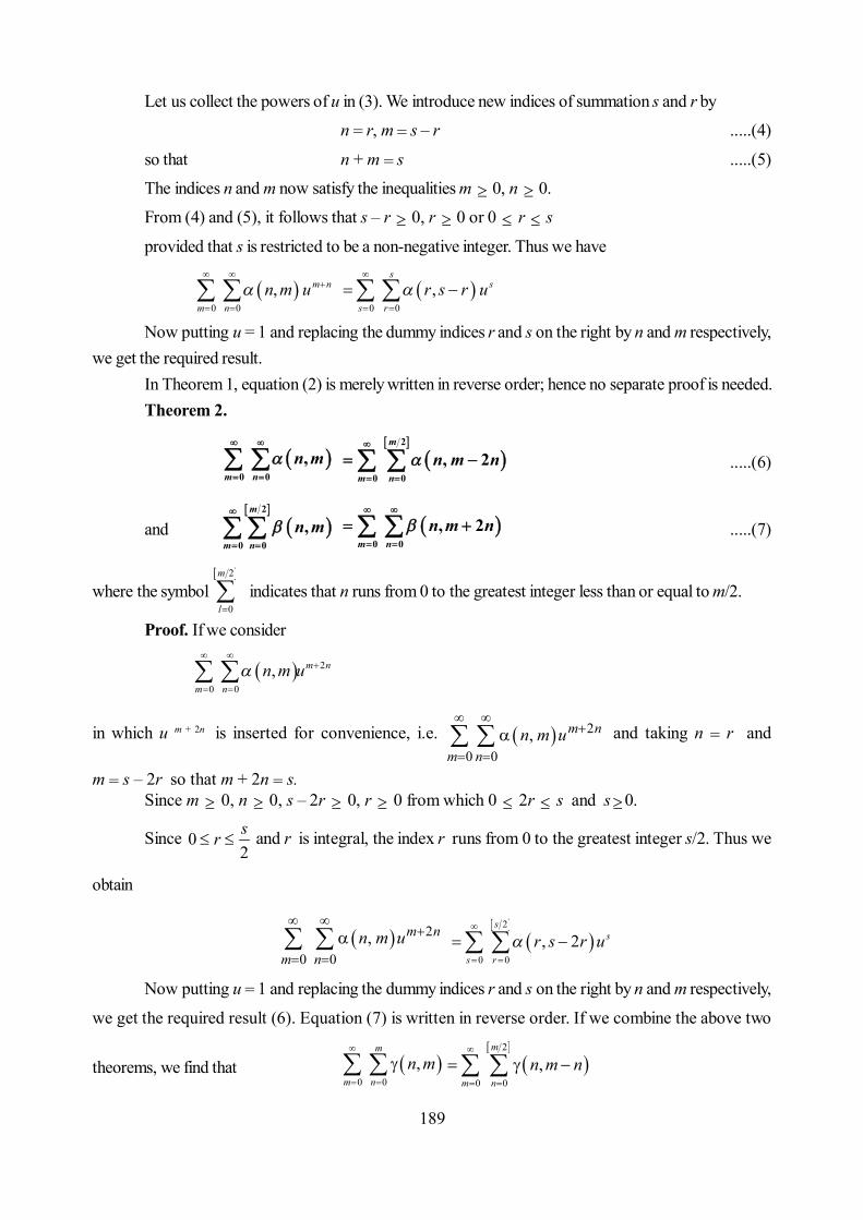
189
Let us collect the powers of u in (3). We introduce new indices of summation s and r by
n = r, m = s – r .....(4)
so that n + m = s .....(5)
The indices n and m now satisfy the inequalities m 0, n 0.
From (4) and (5), it follows that s – r 0, r 0 or 0 r s
provided that s is restricted to be a non-negative integer. Thus we have
0 0
, m n
m nn m u
0 0,
ss
s rr s r u
Now putting u = 1 and replacing the dummy indices r and s on the right by n and m respectively,
we get the required result.In Theorem 1, equation (2) is merely written in reverse order; hence no separate proof is needed.Theorem 2.
m n
n m
0 0,
m
m nn m n
2
0 0, 2 .....(6)
and m
m nn m
2
0 0,
m nn m n
0 0
, 2 .....(7)
where the symbol 2
0
m
l indicates that n runs from 0 to the greatest integer less than or equal to m/2.
Proof. If we consider
2
0 0, m n
m nn m u
in which u m + 2n is inserted for convenience, i.e. 2
0 0, m n
m nn m u
and taking n = r and
m = s – 2r so that m + 2n = s.Since m 0, n 0, s – 2r 0, r 0 from which 0 2r s and s0.
Since 02sr and r is integral, the index r runs from 0 to the greatest integer s/2. Thus we
obtain
2
0 0, m n
m nn m u
2
0 0, 2
ss
s rr s r u
Now putting u = 1 and replacing the dummy indices r and s on the right by n and m respectively,
we get the required result (6). Equation (7) is written in reverse order. If we combine the above two
theorems, we find that 0 0
,m
m nn m
2
0 0,
m
m nn m n
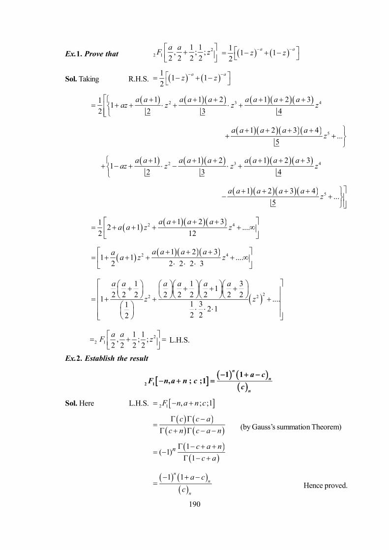
190
Ex.1. Prove that 22 1
1 1, ; ;2 2 2 2a aF z
1 1 12
a az z
Sol. Taking R.H.S. 1 1 12
a az z
2 3 41 1 2 1 2 31 12 2 3 4
a a a a a a a a aaz z z z
51 2 3 4...
5a a a a a
z
2 3 41 1 2 1 2 3
12 3 4
a a a a a a a a aaz z z z
51 2 3 4...
5a a a a a
z
2 41 2 31 2 1 ....2 12
a a a aa a z z
2 41 2 31 1 ....
2 2 2 2 3a a a aa a z z
22 2
1 1 312 2 2 2 2 2 2 2 21 ....1 31 2 1
2 22
a a a a a a
z z
22 1
1 1, ; ;2 2 2 2a aF z
L.H.S.
Ex.2. Establish the result
2 1
1 1, ; ;1
n
n
n
a cF n a n c
c
Sol. Here L.H.S. 2 1 , ; ;1F n a n c
c c ac n c a n
(by Gauss’s summation Theorem)
1( 1)
1n c a n
c a
1 1n
n
n
a cc
Hence proved.

191
Ex.3. Prove that
B(c–) 2F1 (a, b; c; z) 1
112 1
01 , ; ;ct t F a b zt dt
where | z | < 1, > 0, c – > 0.
Sol. Let I = 1
112 1
01 , ; ;ct t F a b zt dt
111
001
rc r r
r r
a b ztt t dt
r
111
0 01
rcrr r
r r
a bz t t dtr
0
rr r
r r
a b r czr c r
0
rr r
r r
a bc zc c r
= B (c–) 2F1 (a, b; c; z)
Ex.4. Show that if b > 0,
2F1(a, b ; 2b ; z)
22 1
2 10
2 1 / 2sin 1 cos 1 cos
2 ,
ab a a
bz
dB b b
where 2z
z
Deduce that
22 1 2 1
1 1 1 1 1, ; 2 ; 2 1 , ; ;2 2 2 2 2
aF a b b z z F a a b
Sol. We know that if | z | < 1 and if Re (c) > Re (b) > 0, then
B (b, c – b) 2F1 (a, b ; c ; z) = 1
11
01 1c b abt t tz dt .....(9)
For c = 2b, it reduces to
2F1 (a, b; 2b; z) 1
11
0
1 1 1,
b abt t tz dtB b b
.....(10)
Putting t = sin2 , we have
2F1 (a, b ; 2b ; z) 2
2 1 2 1 2
0
2 sin cos 1 sin,
ab b z dB b b

192
2
2 1 2 1
0
2 1 cos 2sin cos 1, 2
ab b z d
B b b
2
2 1 2 1
0
2 2 cos 2sin cos, 2
ab b z z d
B b b
22 1 2 1
0
2 1 2sin cos 1 cos 2
, 2
a ab bz z d
B b b z
2
2 12 1
0
2 1 2sin 2 1 cos 2
2 ,
ab a
bz
dB b b
.....(11)
where 2
zz
. If we put 2= , then (11) becomes
2F1 (a, b; 2b; z)
2 1
2 10
1 2sin 1 cos
2 ,
ab a
bz
dB b b
.....(12)
In the same way, if we substitute t = cos2in (10), we get
2F1 (a, b; 2b; z)
2 1
2 10
1 2sin 1 cos
2 ,
ab a
bz
dB b b
.....(13)
Adding (12) and (13) and applying the property of the definite integral, viz.
2
00
2 , if 2 ,
0, if 2
aa f x dx f a x f x
f x dx
f a x f x
we obtain the desired result
2F1 (a, b; 2b; z)
22 1
2 10
1 2sin 1 cos 1 cos
2 ,
ab a a
bz
dB b b
To deduce the second part, we find from example 1 that
2 22 1
1 11 cos 1 cos 2 , ; ; cos2 2 2 2
a a a aF
Hence 2F1 (a, b; 2b; z)
22 1 2 2
2 12 10
4 1 2 1 1sin , ; ; cos2 2 2 22 ,
ab
bz a aF dB b b
Expanding 2F1 (2 cos2) in terms of its series and integrating with the help of beta function
formula, we have

193
2F1 (a, b; 2b; z)
22 2 1 2
2 10 0
2 1 24 1 2sin cos
1 22 ,
ar r b rr
br r
a azd
rB b b
22 1
0
2 1 24 1 2 1 21 2 2 1 22 ,
ar rr
br r
a az b rr b rB b b
Applying Legendre’s duplication formula, we get
2
0
122
2 1122
a rrr
rr
aaz
rb
2F1 (a, b; 2b; z) 22 1
1 12 1 , ; ;2 2 2 2 2
az a aF b
Ex.5. Show that if x2 2
,
sin nx = n sin x 2F1 n n x21 1 1 1 3, ; ; sin
2 2 2 2 2
and n nnx F x22 1
1cos , ; ; sin2 2 2
.
Sol. We know that sin nx and cos nx satisfy the following differential equation
22
2 0d y n ydx
.....(14)
Let us transform (14) by the substitution u = sin2 x. Then
dudx
2
2sin 2 and 2cos 2d ux xdx
Now,dydx
sin 2dy du dyxdu dx du
2
2d ydx
sin 2d dy d dyxdx dx dx du
2
22cos 2 sin 2dy d y dux xdu dxdu
22
22cos 2 sin 2dy d yx xdu du
2
2 2 222 1 2sin 4sin cosdy d yx x x
du du

194
2
2d ydx
2
22 1 2 4 1dy d yu u udu du
Substituting the value of 2
2d ydx
in (14), it becomes
2 2
211 02 4
d y dy nu u u ydudu
The above equation may be written as
2
211 1 02 2 2 2 2
d y n n dy n nu u u ydudu
which is a Gauss’s hypergeometric equation with 1, ,
2 2 2n na b c
. Hence the general solution of
(14) is given by
2 22 1 2 1
1 1 1 1 1 3, ; ; sin sin , ; ; sin2 2 2 2 2 2 2 2n ny A F x B x F n n x
Since sin nx is the solution
2 2
2 1 2 11 1 1 1 1 3sin , ; ; sin sin , ; ; sin
2 2 2 2 2 2 2 2n nnx A F x B x F n n x
.....(15)
For x = 0, equation (15) gives A = 0Further
sinsin
nxx
22 1
1 1 1 1 3, ; ; sin2 2 2 2 2
B F n n x
Now taking limit of both sides as 0x , and noting that 0
sinlim 1
,
we get B = n
sin nx = 22 1
1 1 1 1 3sin , ; ; sin2 2 2 2 2
n x F n n x
Again, if y = cos nx, then putting x = 0, we see that A = 1, and on differentiating and putting x = 0,we get B = 0, which establishes the second part.
Ex.6. Show that
1 12 1
0 0
1, ; ; cosh 2
2u a ba b F a b z e u z u v du dv
provided Re (a) > 0 and Re (b) > 0.
Sol. R.H.S 1 1
0 0cosh 2u a be u z u v du dv
.....(16)

195
But we know that 2
0
2cosh 22
r r r r
r
u v zu zr
Putting this value in the above integral (16), then it breaks up into product of two integrals, and wehave
21 1
0 0 0
22
r ru a r v b r
r
z e u du e v dvr
2
0
22 1
rr
ra r b r z
r
2
0
212 22
rrr r
r
a a b bz
r r
2 1
2 10
122
122
r rr r
rr
a a b b z
r r r
(applying Legendre’s duplication formula)
0 12
rr r
rr
a b za b
r
2 11, ; ; . .2
a b F a b z L H S
Ex.7. Prove that
11 12 1 2 1
1lim , ; ; 1, 1 ; 2 ;
1nn n
c n
a bF a b c z z F a n b n n z
c n
Sol. L.H.S = 2 11lim , ; ;
c nF a b c z
c
0
1limr
r rc n r r
a b zc c r
0
limr
r rc n r
a b zc r r
1
rr r
r n
a b zn r r

196
11 1
0 1 1
s ns n s n
s
a b zs s n
(Putting r – n – 1 = s)
11 1
0
1 12 1
s ns n s n
s s
a n a b n b zs n n
11 1
0
1 11 2
n sn n s s
s s
a b z a n b n zn n s
11 1
2 1 1, 1 ; 2 ;1
nn na bz F a n b n n z
n
= R.H.SEx.8. It the complete elliptic integral of first kind being
2
0 2 21 sin
dKk
Show that 22 1
1 1, ; 1 ;2 2 2
K F k
Sol. We have2
2 20 1 sin
dKk
Putting sin t
then cosd = 1 12
dtt
or d = 1 1 12 1
dtt t
K 1 1 21 21 2 2
0
1 1 12
t t k t dt
By integral representation of 2F1 (a, b ; c ; z), we have
K
22 1
1 111 1 12 2 , ; 1 ;2 1 2 2
F k
22 1
1 1, ; 1 ; . .2 2 2
F k R H S
Ex.9. Prove that
1
112 1
0
1, ; ; 1 1 ,, ,
c b abF a b c z u u zu duB b c b
where c > b > 0. Hence prove that
21
2 1 1,2 ; 3 ; log 1zzF z e z
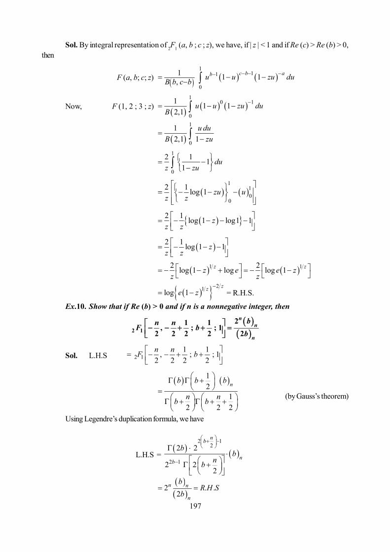
197
Sol. By integral representation of 2F1 (a, b ; c ; z), we have, if | z | < 1 and if Re (c) > Re (b) > 0,then
F (a, b; c; z) 1
11
0
1 1 1,c b abu u zu duB b c b
Now, F (1, 2 ; 3 ; z) 1
0 1
0
1 1 12,1
u u zu duB
1
0
12,1 1
u duB zu
1
0
2 1 11
duz zu
1
10
0
2 1 log 1 zu uz z
2 1 log 1 log1 1zz z
2 1 log 1 1zz z
1 12 2log 1 log log 1z zz e e zz z
21log 1zze z
= R.H.S.
Ex.10. Show that if Re (b) > 0 and if n is a nonnegative integer, then
2 1
21 1, ; ; 12 2 2 2 2
nn
n
bn nF bb
Sol. L.H.S 2 11 1, ; ; 1
2 2 2 2n nF b
12
12 2 2
nb b b
n nb b
(by Gauss’s theorem)
Using Legendre’s duplication formula, we have
L.H.S =
2 12
2 1
2 2
2 22
nb
nb
bb
nb
2 . .2
n n
n
bR H S
b
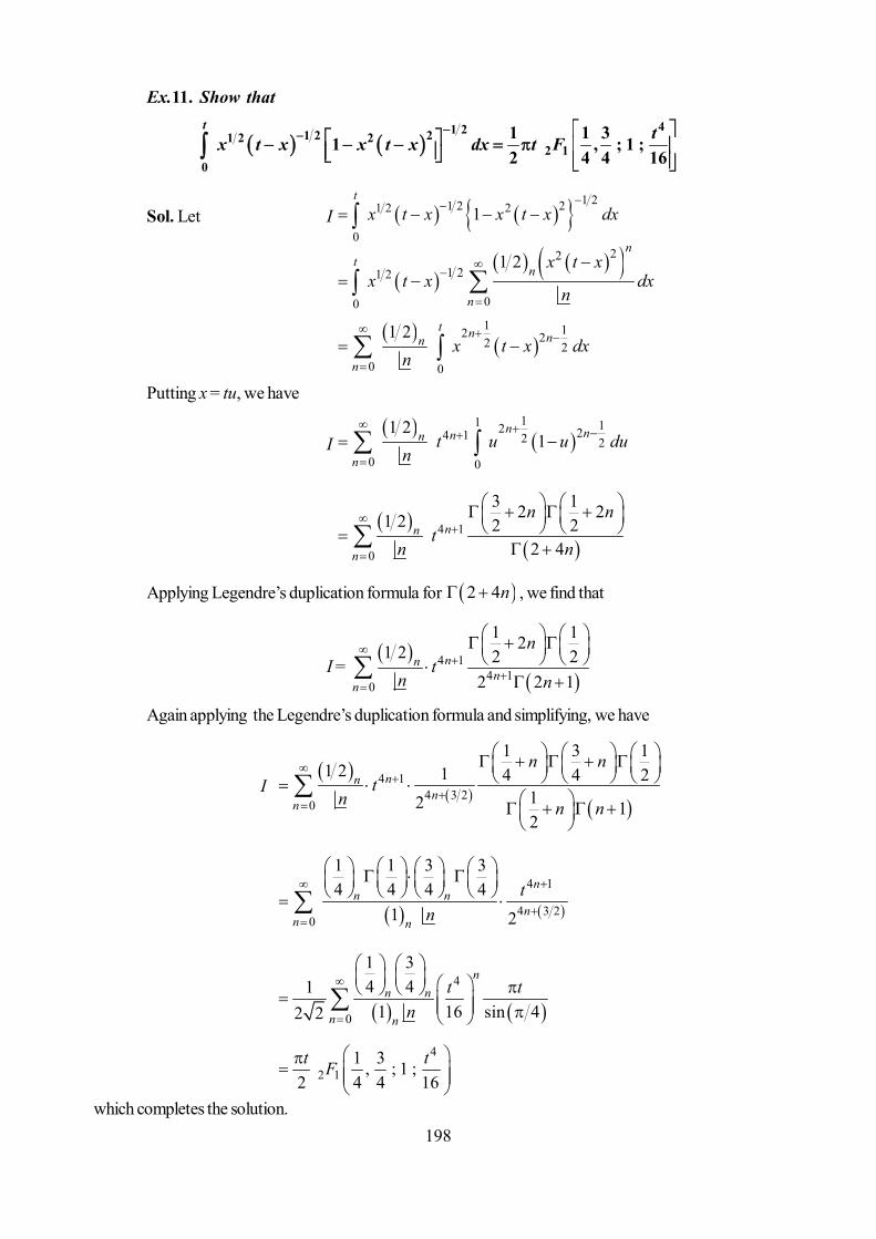
198
Ex.11. Show that
41 21 2 21 2 2
2 10
1 1 31 , ; 1 ;2 4 4 16
t tx t x x t x dx t F
Sol. Let I 1 21 2 21 2 2
0
1t
x t x x t x dx
22
1 21 2
00
1 2n
tn
n
x t xx t x dx
n
1 12 22 20 0
1 2 t n nn
nx t x dx
n
Putting x = tu, we have
I
11 12 24 1 2 2
0 0
1 21
n nnn
nt u u du
n
4 1
0
3 12 21 2 2 22 4
nn
n
n nt
n n
Applying Legendre’s duplication formula for 2 4n , we find that
I =
4 1
4 10
1 121 2 2 22 2 1
nnn
n
nt
n n
Again applying the Legendre’s duplication formula and simplifying, we have
I
4 14 3 2
0
1 3 11 2 1 4 4 2
12 12
nnn
n
n nt
n n n
4 1
4 3 20
1 1 3 34 4 4 4
1 2
nn n
nn n
tn
4
0
1 34 41
1 16 sin 42 2
nn n
n n
t tn
4
2 11 3, ; 1 ;
2 4 4 16t tF
which completes the solution.
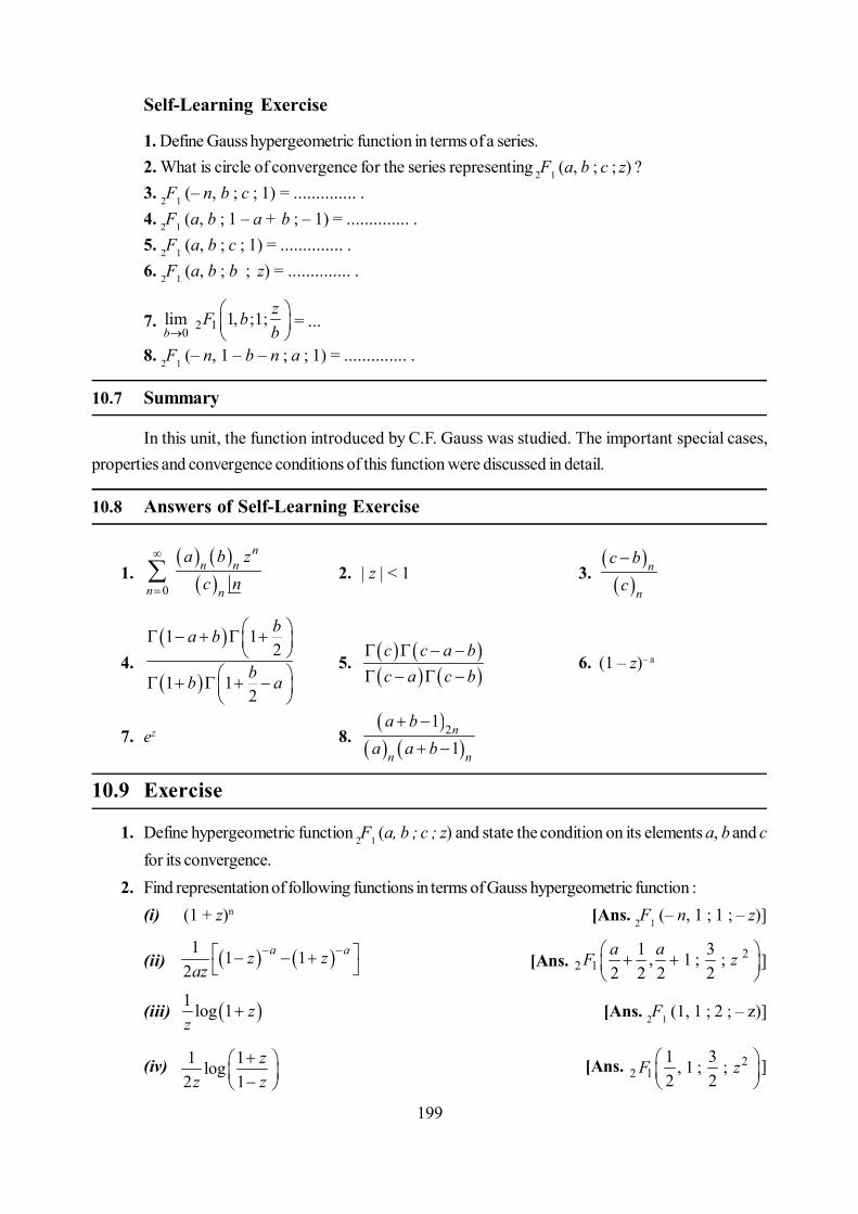
199
Self-Learning Exercise
1. Define Gauss hypergeometric function in terms of a series.2. What is circle of convergence for the series representing 2F1 (a, b ; c ; z) ?3. 2F1 (– n, b ; c ; 1) = .............. .4. 2F1 (a, b ; 1 – a + b ; – 1) = .............. .5. 2F1 (a, b ; c ; 1) = .............. .6. 2F1 (a, b ; b ; z) = .............. .
7. 2 10lim 1, ;1;b
zF bb
= ...
8. 2F1 (– n, 1 – b – n ; a ; 1) = .............. .
10.7 Summary
In this unit, the function introduced by C.F. Gauss was studied. The important special cases,properties and convergence conditions of this function were discussed in detail.
10.8 Answers of Self-Learning Exercise
1.
0
nn n
n n
a b zc n
2. | z | < 1 3.
n
n
c bc
4.
1 12
1 12
ba b
bb a
5. c c a bc a c b
6. (1 – z)– a
7. ez 8.
211n
n n
a ba a b
10.9 Exercise
1. Define hypergeometric function 2F1 (a, b ; c ; z) and state the condition on its elements a, b and cfor its convergence.
2. Find representation of following functions in terms of Gauss hypergeometric function :(i) (1 + z)n [Ans. 2F1 (– n, 1 ; 1 ; – z)]
(ii) 1 1 12
a az zaz
[Ans. 2
2 11 3, 1 ; ;
2 2 2 2a aF z
]
(iii) 1 log 1 zz
[Ans. 2F1 (1, 1 ; 2 ; – z)]
(iv) 1 1log2 1
zz z
[Ans. 22 1
1 3, 1 ; ;2 2
F z
]
200
(v)1sin z
z
[Ans. 2
2 11 1 3, ; ;2 2 2
F z
]
(vi) 11 tan zz
[Ans. 22 1
1 3,1 ; ;2 2
F z
]
(vii) sin z [Ans. 20 1
3 1; ;2 4
z F z
]
(viii)cos z [Ans. 20 1
1 1; ;2 4
F z
]
3. Express complete elliptic integral of the second kind in terms of Gauss’s hypergeometric function
[Ans. 22 1
1 1 1, ; 1 ;2 2 2
F k
]
4. By transforming the equation 2
22 0d y n y
dx to hypergeometric form by the substitution 2sin z ,
prove that if 0 z then,
22 1
1cos cos , ; ; cos sin cos2 2 2 2 2
n n n nnz F z n z
22 1
1 1 3, ; ;cos2 2 2 2 2
n nF z
and 22 1
1sin sin , ; ;cos cos cos2 2 2 2 2
n n n nnz F z n z
22 1
1 1 3, ; ; cos2 2 2 2 2
n nF z
5. Establish the transformation formula
2F1 (2a, 2b; a + b + 12 ; z) = 2F1 {a, b; a + b +
12 ; 4z (1 – z)}
provided that a + b + 12 is not zero or a negative integer and if | z | < 1 and | 4z (1 – z) | < 1
6. Show that
2 11
, ; ;lim
log 1z
F a b a b z a bz a b
7. If the complete elliptic integral of the first kind is 2 1 22 2
0
1 sin ,K k d
then show that 22 1
1 1, ;1; , | | 12 2 2
K F k k
201
Unit 11 : Gauss and Confluent Hypergeometric FunctionsStructure of the Unit
11.0 Objective
11.1 Introduction
11.2 Linear Transformation Formulas for Hypergeometric Function
11.2.1 Applications
11.3 Differentiation Formulas for Hypergeometric Function
11.4 Linear Relation between solutions of Hypergeometric Equations
11.5 Relations of Contiguity for Hypergeometric Function
11.6 Kummer’s Confluent Hypergeometric Function
11.6.1 Convergency
11.6.2 Differentiation Formulas
11.6.3 Integral Representation
11.6.4 Kummer’s First Transformation
11.7 Summary
11.8 Answers of Self-Learning Exercise
11.9 Exercise
11.0 Objective
In the last unit the Gauss hypergeometric function was introduced and some properties, summa-tion theorems and convergence conditions for this function were discussed. The aim of this unit is tostudy further the hypergeometric function. Precisely you will study the linear transformation formulas, con-tiguous function relations, differentiation formulas and a linear relation between the solutions of hyper-geometric differential equation. You will also study the kummer’s confluent hypergeometric function andimportant formulas concerned with this function.
11.1 Introduction
Here some more results for the Gauss hypergeometric function (introduced in the last unit) willbe established. In fact linear transformation formulas, contiguous function relations, differentiation formu-las etc. will be discussed in this unit.Next, the Kummer’s confluent hypergeometric function will be intro-duced and important formulas for this function will also be established.
202
11.2 Linear Transformation Formulas
Result :
If z 1 and z
z
1
1, then
(i) a zF a b c z z F a c b cz
2 1 12, , ; 1 , , ;
1.....(1)
(ii) b zF a b c z z F c a b cz
2 1 12, , ; 1 , ; ;
1.....(2)
(iii) c a bF a b c z z F c a c b c z 2 1 12, , ; 1 , ; ; .....(3)
Proof. (i) We know that by integral representation of 2 1 , , ;F a b c z , if | z | < 1 and if
Re Re 0c b
Then 2 1, , ; ;B b c b F a b c z 1 110
1 1c b abt t tz dt
1 110
1 1 1 1 1c bb at t z t dt
1 110
1 1b ac bt t z tz dt
1 110
1 1 11
aa bc b tzz t t dt
z
2 11 , , ; ;1
a zz B c b b F a c b cz
Thus 2 1 , ; ;F a b c z 2 11 , ; ;1
a zz F a c b cz
(ii) Taking L.H.S 2 1 , ; ;F a b c z 2 1 , ; ;F b a c z
2 11 ; ; ;1
b zz F b c a cz
(by first transformation formula)
2 11 ; ;1
b zz F c a b cz
(by symmetric properly)
Hence 2 1 , ; ;F a b c z 2 11 , ; ;1
b zz F c a b cz
(iii) From (1), we have 2 1 , ; ;F a b c z 2 11 , ; ;1
a zz F c b a cz
.....(4)
203
Putting1
z yz
or 1 - y = (1 – z)-1, we have
Now 2 1 , ; ;1
zF c b a cz
= 2 1 , ; ; ;F c b a c y
2 11 , ; ;
1c b yy F c b c a c
y
.....(5)
or 2 1 , ; ;1
zF c b a cz
2 11 , ; ;c bz F c b c a c z ......(6)
Using (6) in (4), we have
2 1 , ; ;F a b c z 2 11 , ; ;c a bz F c a c b c z
11.2.1 Applications
If we set 12
z in the first transformation formula, then
2 11, ; ;2
F a b c 2 12 , ; ; 1a F a c b c .....(7)
The series on the R.H.S. of (7) can be summed in terms of product of gamma functions with thehelp of Kummer’s theorem in the following cases :
(i) 1c c a b that is 1b a
(ii) 1c a a b or 1
2a bc
From the first case, we get
2 11,1 ; ;2
F a a c
2 12 , 1 ; ; 1a F a c a c
2 11,1 ; ;2
F a a c
122
12
a c ac
c ac a
Further, applying the Legendre’s duplication formula for c and c a , then we obtain
2 11,1 ; ;2
F a a c
12 2
12 2
c c
c a c a
In the same way, in the second case, we can prove the following result.
2 11 1, ; ;
2 2a bF a b
1 12 21 1
2 2
a b
a b

204
11.3 Differentiation of Hypergeometric Functions
Result : Show that
(i) d F a b c xdx
2 1 , ; ; ab F a b c xc
2 1 1, 1; 1 ; .....(1)
(ii) n
nd F a b c xdx
2 1 , ; ; n n
n
a bF a n b n c n x
c 2 1 , ; ; .....(2)
Proof of (i), we have
2 1 , ; ;d F a b c xdx
0
rr r
r r
a bd xdx c r
1
0
rr r
r r
a b r xc r
1
1 1rr r
r r
a bx
c r
1 1
0 1
nn n
n n
a b xc n
Since 1na 1 na a ,
Therefore 2 1 , ; ;d F a b c xdx
0
1 11
nn n
n n
a a b b xc c n
2 1 , ; ;d F a b c xdx
2 1 1, 1 ; 1 ;ab F a b c xc
(ii) We prove the result by the principle of mathematical inductionSince by (1), we have
2 1 , ; ;d F a b c xdx
2 1 1, 1 ; 1 ;a b F a b c xc
Therefore the result (2) is true for n = 1Suppose that (2) is true for n = m (a fixed positive integer) i.e.
2 1 , ; ;m
md F a b c xdx
2 1 , ; ;m m
m
a bF a m b m c m x
c
Now, 1
2 11 , ; ;m
md F a b c xdx
2 1 , ; ;
m
md d F a m b m c m xdx dx
2 1 , ; ;m m
m
a b d F a m b m c m xc dx
[by equation (4)]
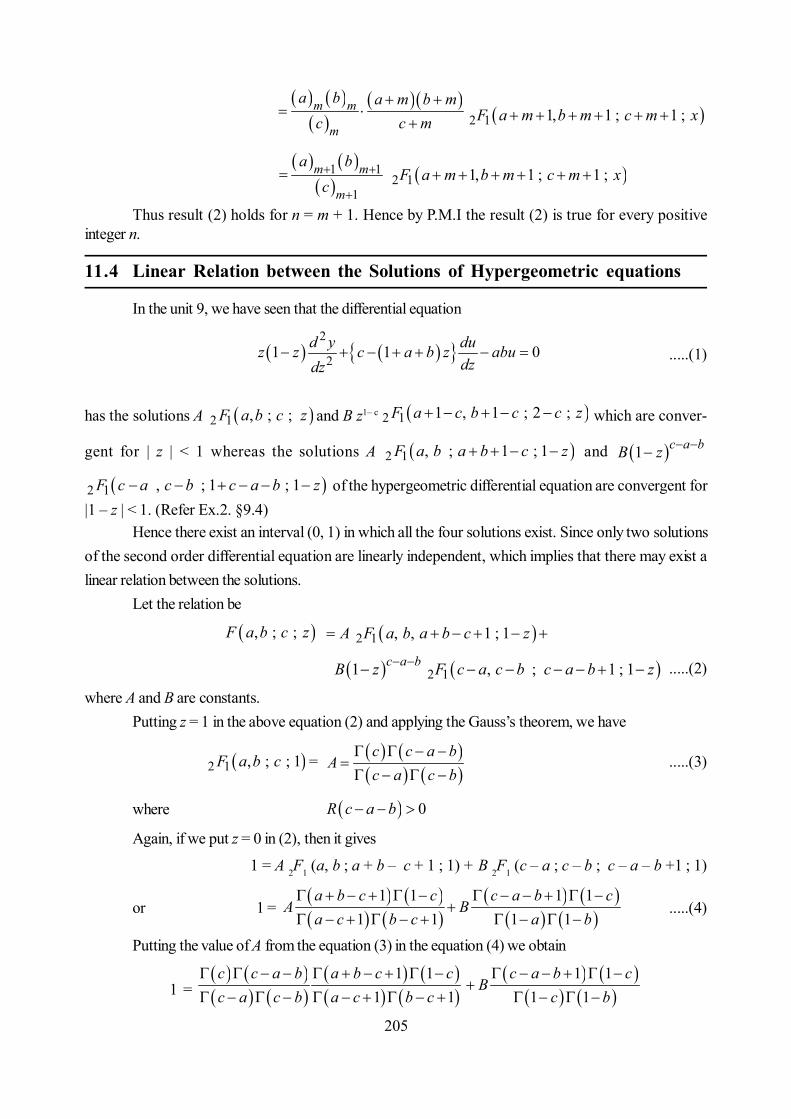
205
m m
m
a b a m b mc c m
2 1 1, 1 ; 1 ;F a m b m c m x
1 1
1
m m
m
a bc
2 1 1, 1 ; 1 ;F a m b m c m x
Thus result (2) holds for n = m + 1. Hence by P.M.I the result (2) is true for every positiveinteger n.
11.4 Linear Relation between the Solutions of Hypergeometric equations
In the unit 9, we have seen that the differential equation
2
21 1 0d y duz z c a b z abudzdz
.....(1)
has the solutions A 2 1 , ; ;F a b c z and B z1– c 2 1 1 , 1 ; 2 ;F a c b c c z which are conver-
gent for | z | < 1 whereas the solutions A 2 1 , ; 1 ; 1F a b a b c z and 1 c a bB z
2 1 , ; 1 ; 1F c a c b c a b z of the hypergeometric differential equation are convergent for|1 – z | < 1. (Refer Ex.2. §9.4)
Hence there exist an interval (0, 1) in which all the four solutions exist. Since only two solutionsof the second order differential equation are linearly independent, which implies that there may exist alinear relation between the solutions.
Let the relation be
, ; ;F a b c z 2 1 , , 1 ; 1A F a b a b c z
2 11 , ; 1 ; 1c a bB z F c a c b c a b z .....(2)
where A and B are constants.Putting z = 1 in the above equation (2) and applying the Gauss’s theorem, we have
2 1 , ; ; 1F a b c = c c a b
Ac a c b
.....(3)
where 0R c a b
Again, if we put z = 0 in (2), then it gives
1 = A 2F1 (a, b; a+b – c+ 1 ; 1) + B 2F1 (c – a; c–b ; c– a – b +1 ; 1)
or 1 =
1 1 1 11 1 1 1
a b c c c a b cA B
a c b c a b
.....(4)
Putting the value of A from the equation (3) in the equation (4) we obtain
1 =
1 11 1
c c a b a b c cc a c b a c b c
1 11 1
c a b cB
c b

206
or 1 =
1 11 1
c c c a b c a bc a c a c b c b
1 11 1
c a b cB
a b
Since 1sin
z zz
, therefore
1 =
sin sinsin sin
c a c bc c a b
1 11 1
c a b cB
a b
1 1
1 1c a b c
Ba b
=
sin sin1
sin sinc a c bc c a b
sin sin sin sinsin sin
c c a b c a c bc c a b
cos cos 2 cos cos 22sin sin
a b c a b b a c a bc c a b
cos cos2sin sin
a b b ac c a b
sin sin
sin sina b
c c a b
B =
1 1 sin sin
1 1 sin sina b a b
c c a b c a b c
Applying sin z = 1z z
, we have
B =
1 1
1 1 1 1a b
c c a b a a b b
21 1c c a b c a b c
B =
c a b c
a b
Substituting these values of A and B in (2), we get the following linear relation :
F (a; b; c; z ) = c c a b
F a b a b c zc a c b
2 1 , ; 1 ; 1
c a bc a b cz F c a c b c a b z
a b
2 11 , ; 1 ; 1
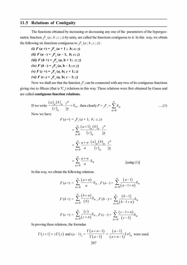
207
11.5 Relations of Contiguity
The functions obtained by increasing or decreasing any one of the parameters of the hypergeo-metric function 2F1 (a; b; c; z) by unity, are called the functions contiguous to it. In this way, we obtainthe following six functions contiguous to 2F1 (a; b; c; z) :
(i) F (a+) = 2F1 (a+ 1 ; b; c; z)(ii) F (a–) = 2F1 (a– 1, b; c; z)(iii) F (b+) = 2F1 (a, b + 1; c; z)(iv) F (b–) = 2F1 (a, b – 1; c; z)(v) F (c+) = 2F1 (a b; c + 1; z)(vi) F (c–) = 2F1 (a b; c – 1; z)Now we shall see that the function 2F1 can be connected with any two of its contiguous functions
giving rise to fifteen (that is 6C2) relations in this way. These relations were first obtained by Gauss andare called contiguous function relations.
If we write
nn n
nn
a b zc n
, then clearly F = 2F1 0
nn
.....(1)
Now we haveF (a +) = 2F1 (a + 1; b; c; z)
0
1 nn n
n n
a b zc n
0
nn n
n n
a ba n za c n
0n
n
a na
[using (1)]
In this way, we obtain the following relations
F (a +) =
0n
n
a na
, F (a –) =
0
11 n
n
aa n
F (b +) = 0
nn
b nb
, F (b –) =
0
11 n
n
bb n
F (c +) =
0n
n
cc n
, F (c –) = 0
11 n
n
c nc
In proving these relations, the formulae
1z z z and (a – 1)n =
11
a na
=
11 n
aa
a n
were used.
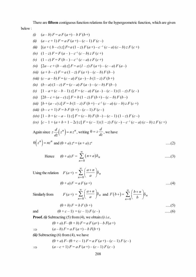
208
There are fifteen contiguous function relations for the hypergeometric function, which are givenbelow :
(i) (a – b) F = a F (a +) – b F (b +)(ii) (a – c + 1) F = a F (a +) – (c – 1) F (c –)(iii) [(a + ( b – c) z] F=a (1 – z) F (a +) – c –1 (c – a) (c – b) z F (c +)(iv) (1 – z) F = F (a – ) – c–1 (c – b) z F (c +)(v) (1 – z) F = F (b – ) – c–1 (c – a) z F (c +)(vi) [2a – c + (b – a) z] F = a (1 – z) F (a +) – (c – a) F (a –)(vii) (a + b – c) F = a (1 – z) F (a +) – (c – b) F (b –)(viii) (c – a – b) F = (c – a) F (a –) – b (1 – z) F (b +)(ix) (b – a) (1 – z) F = (c – a) F (a –) – (c – b) F (b –)(x) [1 – a + (c – b – 1) z] F = (c – a) F (a –) – (c – 1) (1 – z) F (c –)(xi) [2b – c + (a – c) z] F = b (1 – z) F (b +) – (c – b) F (b –)(xii) [b + (a – c) z] F = b (1 – z) F (b +) – c–1 (c – a) (c – b) z F (c +)(xiii) (b – c + 1) F = b F (b +) – (c – 1) F (c –)(xiv) [1 – b + (c – a – 1) z] F = (c – b) F (b –) – (c – 1) (1 – z) F (c –)(xv) [c – 1 + (a + b + 1 – 2c) z] F = (c – 1) (1 – z) F (c –) – c– 1 (c – a) (c – b) z F (c +)
Again since n ndz z n zdz
, writing dzdz
, we have
n nz nz and ( + a) zn = (n + a) zn .....(2)
Hence ( + a) F = 0
nn
n a
......(3)
Using the relation F (a +) =0
nn
a na
( + a) F = a F (a +) .....(4)
Similarly from F (a +) =0
nn
a na
and 0
nn
b nF bb
( + b) F = b F (b +) .....(5)and ( + c – 1) = (c – 1) F (c –) ......(6)Proof. (i) Subtracting (5) from (4), we obtain (i) i.e.,
(+ a) F– (+b) F = aF (a+) – b F(a+) (a–b) F = aF (a+) – bF(b+)(ii) Subtracting (6) from (4), we have
(+a) F– (+ c – 1) F = aF (a+) – (c – 1) F (c –) (a– c + 1) F = aF (a+) – (c – 1) F (c –)
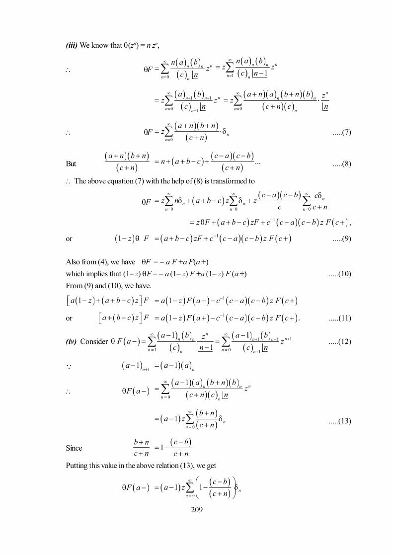
209
(iii) We know that (zn) = n zn,
F 0
nn n
n n
n a bz
c n
1 1
nn n
n n
n a bz z
c n
1 1
0 1
nn n
n n
a bz z
c n
0
nn n
n n
a n a b n b zzc n c n
F
0n
n
a n b nz
c n
.....(7)
But
a n b n
c n
...
c a c bn a b c
c n
.....(8)
he above equation (7) with the help of (8) is transformed to
F 0 0 0
nn n
n n n
c a c b cz n a b c z zc c n
1z F a b c zF c c a c b z F c ,
or 1 z F 1a b c zF c c a c b z F c .....(9)
Also from (4), we have F = –a F +a F(a +)which implies that (1– z) F = –a (1– z) F +a (1– z) F (a +) .....(10)From (9) and (10), we have.
1a z a b c z F 11a z F a c c a c b z F c
or a b c z F 11 .a z F a c c a c b z F c .....(11)
(iv) Consider
11 1
1 0 1
1 11
nnn n n n
n nn n
a b a bzF a zc n c n
.....(12)
11 na
1 na a
F a
0
1 nn n
n n
a a b n bz
c n c n
0
1 nn
b na z
c n
.....(13)
Sinceb nc n
1c bc n
Putting this value in the above relation (13), we get
F a 0
1 1 nn
c ba z
c n

210
0 0
11 n n
n n
a c b z ca zc c n
F a 11 1a z F c a a b z F c .....(14)But in equation (4), if we write (a – 1) in place of a, we get
F a 1a F a F a .....(15)
Combining the equations (14) and (15), we get the required result (iv).(v) If we interchange aand b in (iv), we obtain (v).The remaining ten relations can be deduced by making use of the above five relations.
11.6 Kummer’s Confluent Hypergeometric Function
The hypergeometric differential equation is
2
21 1 0d u duz z c a b z abudz dz
.....(1)
Replacing z by z /bin (1), we get2
2
11 1 0z d u a duz c z aub dz b dz
.....(2)
Now take the limit as b , the equation (2) reduces to
2
2 0d u duz c z audz dz
.....(3)
whose solution is given by 2 1lim , ; ;b
zF a b cb
.....(4)
The equation (3) is known as the confluent hypergeometric differential equation or Kummer’sequation.
Now,
lim rrb
bb
1 2 .... 1lim
. . .... timesb
b b b b rb b b r
1 2 1lim 1 1 ... 1 1b
rb b b
Hence the solution (4) may be written as
2 1lim , ; ;b
zF a b cb
0
limr
r rb r r
a b zc r b
0
limr
r rrb r r
a bzc r b
1 1
0; ;
rr
r r
a z F a c zc r
The function 1F1(a; c; z) is called the confluent hypergeometric function.
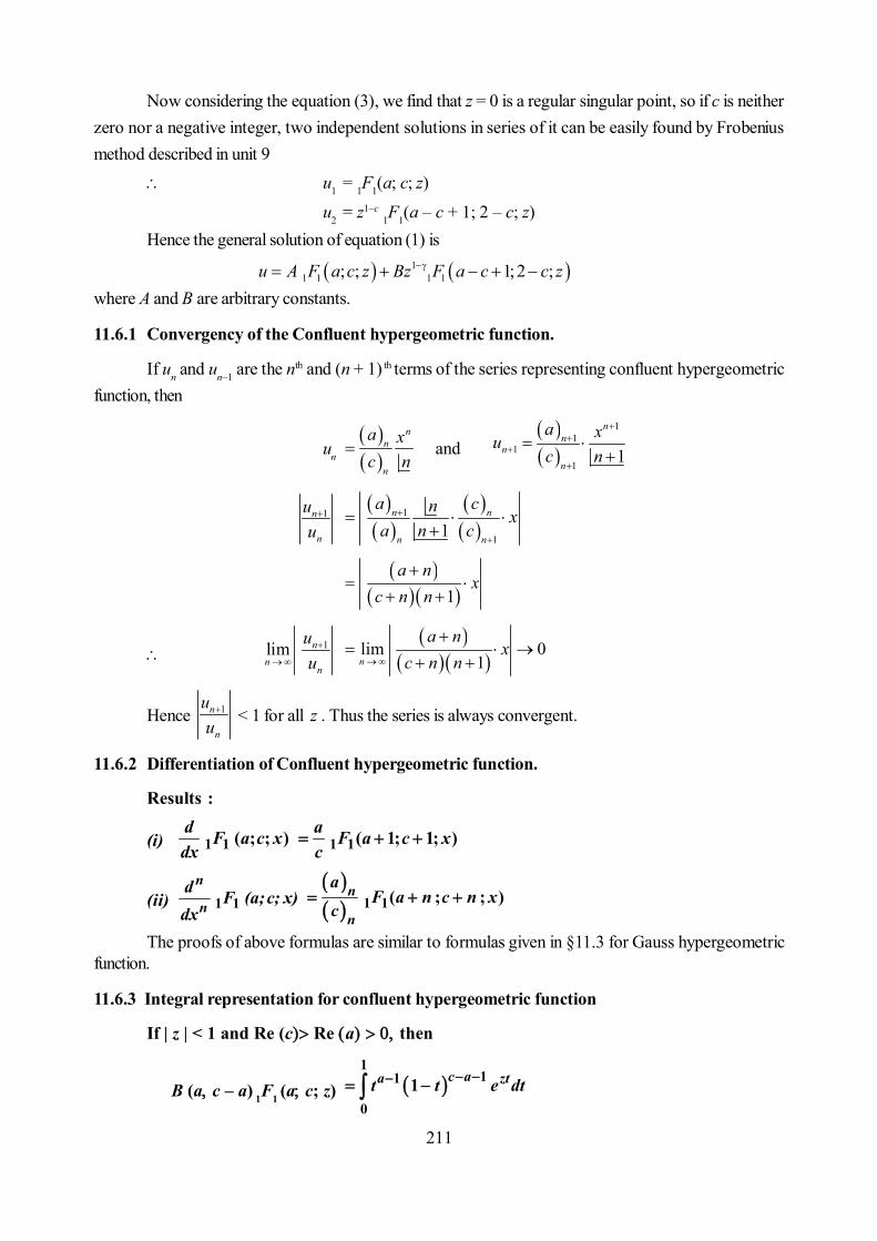
211
Now considering the equation (3), we find that z = 0 is a regular singular point, so if c is neitherzero nor a negative integer, two independent solutions in series of it can be easily found by Frobeniusmethod described in unit 9
u1 = 1F1(a; c; z)
u2 = z1–c 1F1(a – c + 1; 2 – c; z)Hence the general solution of equation (1) is
11 1 1 1; ; 1;2 ;u A F a c z Bz F a c c z
where A and B are arbitrary constants.
11.6.1 Convergency of the Confluent hypergeometric function.
If un and un–1 are the nth and (n + 1) th terms of the series representing confluent hypergeometricfunction, then
un
nn
n
a xc n
and
11
11
1
nn
nn
a xuc n
1n
n
uu
1
11n n
n n
a cn xa n c
1
a nx
c n n
1lim n
nn
uu
lim 01n
a nx
c n n
Hence 1n
n
uu < 1 for all z . Thus the series is always convergent.
11.6.2 Differentiation of Confluent hypergeometric function.
Results :
(i)d F a c xdx 1 1 ( ; ; )
a F a c xc
1 1( 1; 1; )
(ii) 1 1n
nd F (a;c; x)dx
1 1( ; ; )n
n
aF a n c n x
c
The proofs of above formulas are similar to formulas given in §11.3 for Gauss hypergeometricfunction.
11.6.3 Integral representation for confluent hypergeometric function
If | z | < 1 and Re (c Re a then
B (ac – a) 1F1 (ac; z) c aa ztt t e dt 1
11
01

212
or 1F1 (ac z)
c aa ztct t e dt
a c a
111
01
Proof we have R.H.S.
111
001
nc aa
n
c ztt t dt
a c a n
0
n
n
c a n c aza c a n c n
= 1F1 (a; c; z)
11.6.4 Kummer’s first transformation
Result :If c is neither zero nor a negative integer, then 1F1 (a c z) = ez
1F1 (cac z).
Proof : By integral representation of confluent hypergeometric function, we have.
B (acc1F1 (ac z) 1
11
01 c aa ztt t e dt
Using the property of definite integral, we get
1
11
01 cz c a zte t t e dt
= ezB ( c–aa) 1
F1 (c–a; c; – z)
1F1 (a; c; – z) = ez
1F1 (a–c; a; – z)
Ex.1. If m is a positive integer, show that
c ac m a c mc mm
x x dF m a m c x c x xm c dx
11
2 11
, ; ; 1
and deduce that
1 12 2 4 1
2 2 22 1
111 1 1 2 2, ; ; 1
12 2 2 2 22 2
aam m
mm
aa d
F m a ma dm
Sol. R.H.S.
11
0
1 rc ac mc m r
mr
c a m xx x dc xm c rdx
11
0
1 c ac mc m r r
mrm
c a mx x d xc rdx

213
11
0
1 c rc acm r
rm
c r c a m xx xc r
1 1
01 c ac c rr r
r r
c m c a mx x x
c r
121 , ; ;c ax F c m c a m c x
But we know by transformation formula
2F1 (a,bcz) 121 , ; ;c a bz F c a c b c z
R.H.S. = 2F1 (– m, a+ m;c x) = L.H.S.
Deduction. Putting 12
x and 1 ,
2ac
we obtain the second part of the question.
Ex.2. If m is a positive integer, and | x | > 1, show that
2 1 21 2 1, ;1;
2 2m mF
x
1
2
1 1 .1
m m m
mx d
m dx x
Sol. We know that
( )1/ 22
1
1 x+1/ 2
2
111xx
=æ ö÷ç + ÷ç ÷çè ø
1/ 2
21 11x x
-æ ö÷ç= + ÷ç ÷÷çè ø
1/ 22
1
1 x
2 1
0
112
r r
r
r
x
r
Hence 1/ 221m
md xdx
2 1
0
1 12
rmr
mrr
d xrdx
2 1
0
1 1 2 1 2 2 ...... 22
rr m
rrr r r m x
r
2 1
0
1 2 121
r mmm r r
r
r x
r
But (2r + 1)m =
2 12 1
r mr
12 12 2
12
m m mr r
r r
Putting the value of (2r + 1)m in the above relation
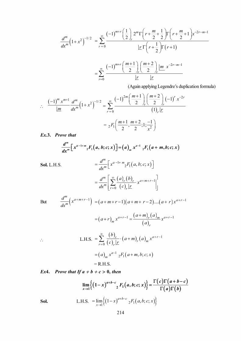
214
1/ 221m
md xdx
2 1
0
1 11 2 12 2 2 2
1 12
m r m r m
r
r
m mr r x
r r r
2 1
0
1 212 2
m r r m
r r
r
m m m x
r r
(Again applying Legendre’s duplication formula)
1 1/ 2211
m m m
mx d x
m dx
2 2
0
1 21 12 2
1
m r r
r r
r r
m m x
r
= 2 1 21 2 1, ;1;
2 2m mF
x
Ex.3. Prove that
1 12 1 2 1, ; ; , ; ;
mm a
m m
d x F a b c x a x F a m b c xdx
Sol. L.H.S. 12 1 , ; ;
ma m
md x F a b c xdx
1
0
ma m rr r
mr r
a bd xc rdx
But 1m
a m rm
d xdx
11 2 .... a ra m r a m r a r x
1 1a r a rr m
mr
a m aa r x x
a
L.H.S. 1
0
a rrr m
r r
ba m a x
c r
12 1 , ; ;a
ma x F a m b c x
= R.H.S.Ex4. Prove that If abc0, then
121
lim 1 , ; ;a b c
x
c a b cx F a b c x
a b
Sol. L.H.S. 2 11lim 1 , ; ;a b c
xx F a b c x
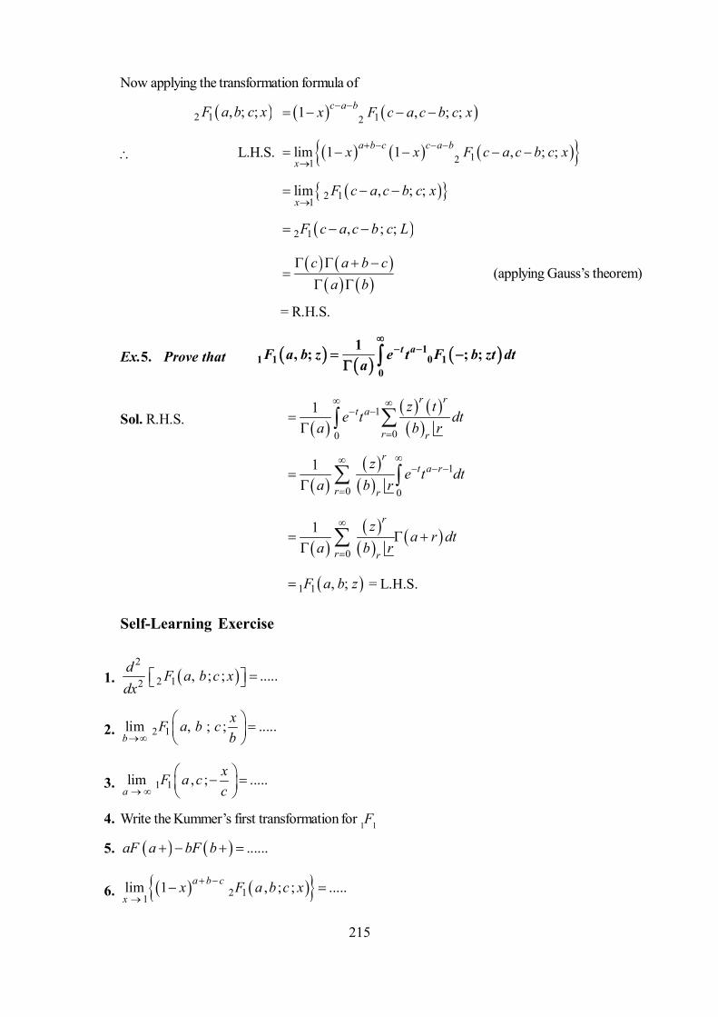
215
Now applying the transformation formula of
2 1 , ; ;F a b c x 121 , ; ;c a bx F c a c b c x
L.H.S. 121lim 1 1 , ; ;a b c c a b
xx x F c a c b c x
2 11lim , ; ;x
F c a c b c x
2 1 , ; ;F c a c b c L
c a b ca b
(applying Gauss’s theorem)
= R.H.S.
Ex.5. Prove that 11 1 0 1
0
1, ; ; ;t aF a b z e t F b zt dta
Sol. R.H.S.
1
00
1 r rt a
r r
z te t dt
a b r
1
0 0
1 rt a r
r r
ze t dt
a b r
0
1 r
r r
za r dt
a b r
1 1 , ;F a b z = L.H.S.
Self-Learning Exercise
1. 2
2 12 , ; ; .....d F a b c xdx
2. 2 1lim , ; ; .....b
xF a b cb
3. 1 1lim , ; .....a
xF a cc
4. Write the Kummer’s first transformation for 1F1
5. ......aF a bF b
6. 2 11lim 1 , ; ; .....a b c
xx F a b c x

216
11.7 Summary
In this unit we established some important formulae such as differentiation formulas, contiguous
function relations, linear relations etc. for Gauss hypergeometric function introduced in the last unit. We
also introduced and studied Kummer’s confluent hypergeometric function.
11.8 Answers to self-Learning Exercise
1. 2 11 1
2, 2; 2;1
a a b bF a b c x
c c
2. 1 1 ; ;F a c x
3. 1 / 21 2c
cx c J z
4. 1 1 1 1; ; ; ;zF a c z e F c a c z
5. a b F
6.
c a b c
a b
11.9 Exercise
1. Prove that 1 1 1 1; ; 1 ; ;n
nx xn nn
db e F a b x b a e F a b n xdx
2. Show that 1 1 2 1; ; lim ; ; ;b
xF a c x F a b cb
3. Show that 1 1 1 1; ; 1 ; ;m
mx xm mm
dc e F a c x c a e F a c m xdx
(Hint. Use Kummer’s first transformation)
4. If incomplete gamma function is defined by 1
0
, , Re 0.x
t aa x e t dt a
Show that 11 1, ; 1; .aa x a x F a a x
5. State Confluent hypergeometric differential equation and explain its solution,6. Prove that
1
1 10
11 2; ; , Re 0,Re 0.
1 12 22 2
zt
aza ztt e F a dt z
a

217
[Hint First replace 1F1 by its integral representation, then change the order of integration, Evalu-ate the inner integral in terms of the gamma function. Write down the remaining integral in termsof
2 1
1 11 2 2, ; ;1
1 122 2
F
aaa
7. Prove that , 1; 1; , ; ; 1, 1; 2;
1a c b x
F a b c x F a b c x F a b c xc c
8. Prove the following relations :
(i) 11, 1; ; , 1, ; , ; 1;
b xF a b c x F a b c x F a b c x
b
(ii) 1, ; ; 1 , ; 1; 1 , ; ;aF a b c x c F a b c x a c F a b c x
9. Show that
(i) 1 1,2;xe x F x
(ii) 1 1; ;xx e F a a xa
10. Prove the following relations
(i) ; ; 1; ; ; 1;bF a b x bF a b x x F a b x
(ii) 1; ; 1 ; 1; 1 ; ;aF a b x b F a b x a b F a b x

218
Unit 12 : Legendre’s Polynomials and Functions Pn(x) and Qn (x)
Structure of the Unit
12.0 Objective
12.1 Introduction
12.2 Legendre’s equation and its Solution
12.3 Definition
12.3.1 Legendre’s Polynomial of Degree n or Legendre’s Function of First Kind
12.3.2 Legendre’s Function of Second Kind
12.3.3 Values of Pn(x) for n = 0, 1, 2, 3, 4, and 5
12.4 Generating Function for Pn(x)
12.5 Rodrigue’s Formulae for Pn(x)
12.5.1 Alternative form of Rodrigue’s Formula
12.5.2 Application
12.6 Orthogonal Property for Pn(x)
12.7 Recurrence Formulas for Pn(x)
12.8 Cristoffel Expansion
12.8.1 Cristoffel Summation Formula
12.9 Expression for Pn(cos ) in Terms of Cosine Series
12.10 Recurrence Formulae for Qn(x)
12.11 Cristoffel’s Second Summation Formula
12.12 Relations Between Pn(x) and Qn(x)
12.13 Summary
12.14 Answer to Self-Learning Exercise
12.15 Exercise
12.0 Objective
Our aim of this unit is to develop the Legendre Polynomials and to discuss its important
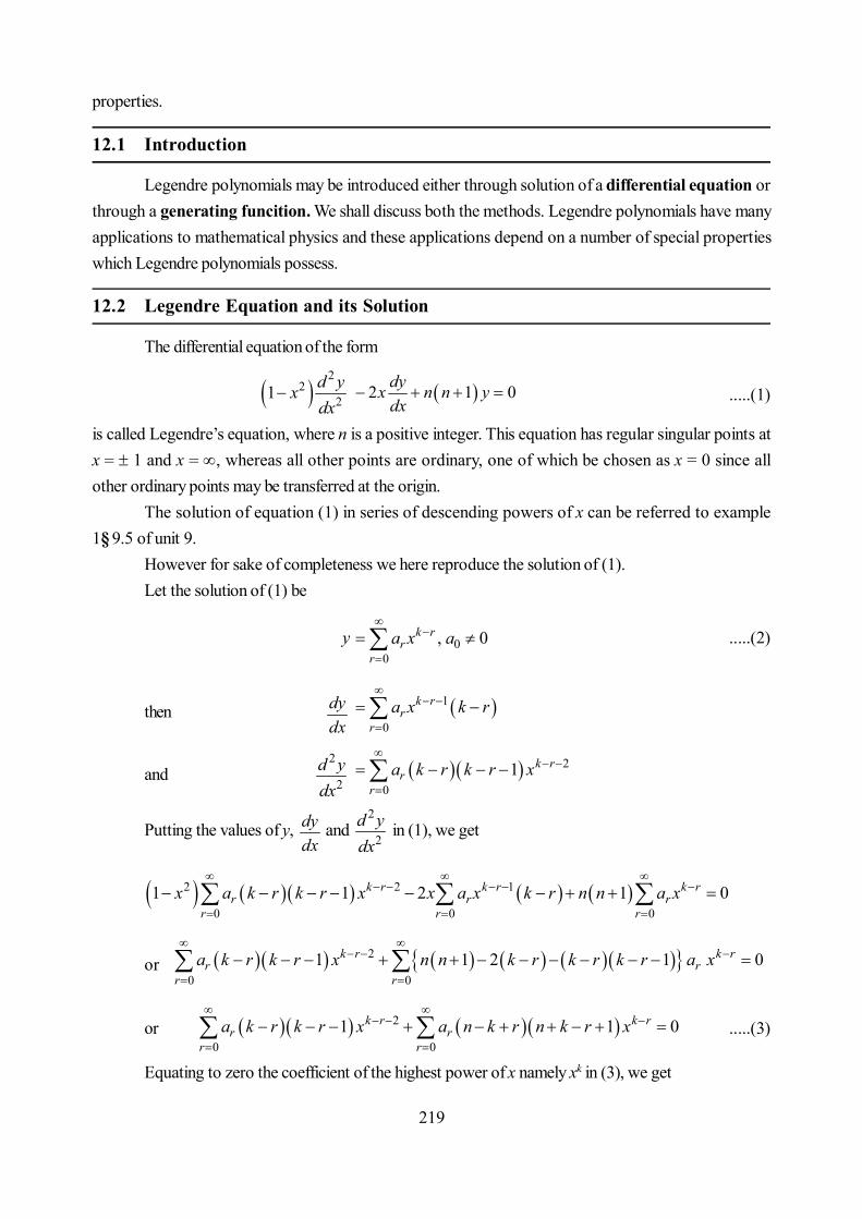
219
properties.
12.1 Introduction
Legendre polynomials may be introduced either through solution of a differential equation orthrough a generating funcition. We shall discuss both the methods. Legendre polynomials have manyapplications to mathematical physics and these applications depend on a number of special propertieswhich Legendre polynomials possess.
12.2 Legendre Equation and its Solution
The differential equation of the form
2
221 d yx
dx 2 1 0dyx n n y
dx .....(1)
is called Legendre’s equation, where n is a positive integer. This equation has regular singular points atx = 1 and x = , whereas all other points are ordinary, one of which be chosen as x = 0 since allother ordinary points may be transferred at the origin.
The solution of equation (1) in series of descending powers of x can be referred to example1§ 9.5 of unit 9.
However for sake of completeness we here reproduce the solution of (1).Let the solution of (1) be
y 00
, 0k rr
ra x a
.....(2)
then dydx
1
0
k rr
ra x k r
and2
2d ydx
2
01 k r
rr
a k r k r x
Putting the values of y, dydx
and 2
2d ydx
in (1), we get
2 2 1
0 0 01 1 2 1 0k r k r k r
r r rr r r
x a k r k r x x a x k r n n a x
or 2
0 01 1 2 1 0k r k r
r rr r
a k r k r x n n k r k r k r a x
or 2
0 01 1 0k r k r
r rr r
a k r k r x a n k r n k r x
.....(3)
Equating to zero the coefficient of the highest power of x namely xk in (3), we get

220
a0 (n – k)(n + k + 1) = 0 k = n, –(n + 1) ( a 0 .....(4)
The next lower power of x is k – 1, so we equate to zero the coefficient of xk – 1 in (3) andobtain
(n – k + 1) (n + k) a1 = 0 .....(5)For k = n and –(n + 1), neither (n – k + 1) nor (n + k) in zero. thesefore a1 = 0Next equating to zero the coefficient of xk – r in (3), we have
(k – r + 2) (k – r + 1) ar –2 + (n – k + r) (n + k – r + 1) ar = 0
ar
22 1
1 rk r k r
an k r n k r
.....(6)
Putting n = 3, 5, 7... in (6) and noting that a1 = 0, we havea1 = a3 = a5 = a7 = ..... = 0 .....(7)
To obtain a2, a4, a6 .... etc, we consider following two casesCase I. When k = n then (6) becomes
ar
22 1
2 1 rn r n r
ar n r
.....(8)
Putting r = 2, 4, 6, .... in (8), we have
a2 0
12 2 1n n
an
a4
2 02 3 1 2 3
4 2 3 2 4 2 1 2 3n n n n n n
a an n n
and so on
Re-writing (2), we have for k = ny = a0x
n + a1xn – 1 + a2x
n – 2 + a3xn – 3 + a4x
n – 4 + ... ....(9)Using (7) and the above values of a2, a4, a4, etc in (9) we get
y
2 40
1 1 2 3....
2 2 1 2 4 2 1 2 3n n nn n n n n n
a x x xn n n
.....(10)
Case II. When k = –( n + 1) then (6) becomes
ar
21
2 1 rn r n r
ar n r
.....(11)
Putting r = 2, 4, 6, .... etc., we get
a2
01 2
2 2 3n n
an
a4
2 0
3 4 1 2 3 44 2 5 2 4 2 3 2 5
n n n n n na a
n n n
and so on.
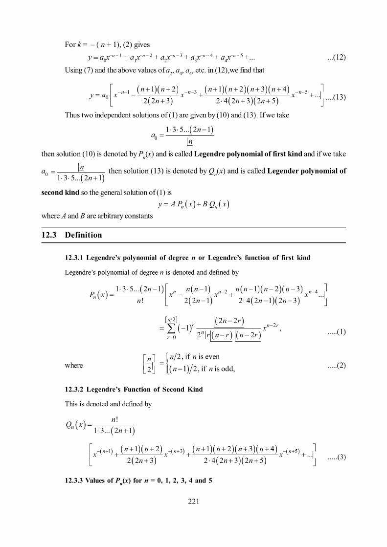
221
For k = – ( n + 1), (2) givesy = a0x
–n – 1 + a1x–n – 2 + a2x
–n – 3 + a3x–n – 4 + a4x
–n – 5 +... ...(12)
Using (7) and the above values of a2, a4, a4, etc. in (12),we find that
1 3 50
1 2 1 2 3 4...
2 2 3 2 4 2 3 2 5n n nn n n n n n
y a x x xn n n
....(13)
Thus two independent solutions of (1) are given by (10) and (13). If we take
a0 1 3 5... 2 1nn
then solution (10) is denoted by Pn(x) and is called Legendre polynomial of first kind and if we take
a0 1 3 5... 2 1n
n
then solution (13) is denoted by Qn(x) and is called Legender polynomial of
second kind so the general solution of (1) is n ny A P x B Q x
where A and B are arbitrary constants
12.3 Definition
12.3.1 Legendre’s polynomial of degree n or Legendre’s function of first kind
Legendre’s polynomial of degree n is denoted and defined by
2 41 3 5... 2 1 1 1 2 3...
! 2 2 1 2 4 2 1 2 3n n n
nn n n n n n n
P x x x xn n n n
22
0
2 21 ,
2 2
nr n r
nr
n rx
r n r n r
.....(1)
where 2n
2, if is even1 2, if is odd,
n nn n
.....(2)
12.3.2 Legendre’s Function of Second Kind
This is denoted and defined by
!
1 3... 2 1nnQ x
n
1 3 51 2 1 2 3 4...
2 2 3 2 4 2 3 2 5n n nn n n n n n
x x xn n n
.....(3)
12.3.3 Values of Pn(x) for n = 0, 1, 2, 3, 4 and 5
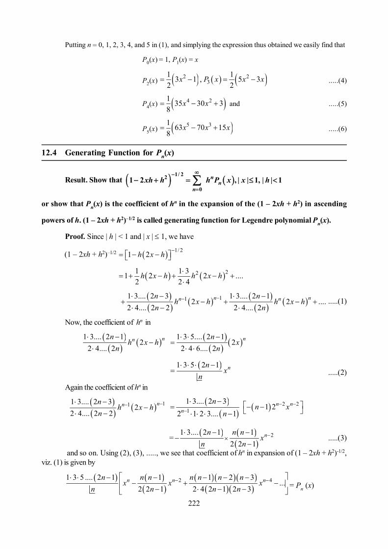
222
Putting n = 0, 1, 2, 3, 4, and 5 in (1), and simplying the expression thus obtained we easily find that
P0(x) = 1, P1(x) = x
P2(x) 2 23
1 13 1 , 5 32 2
x P x x x .....(4)
P4(x) 4 21 35 30 38
x x and .....(5)
P5(x) 5 31 63 70 158
x x x .....(6)
12.4 Generating Function for Pn(x)
Result. Show that 1/ 22
01 2 , | | 1, | | 1n
nn
xh h h P x x h
or show that Pn(x) is the coefficient of hn in the expansion of the (1 – 2xh + h2) in ascending
powers of h. (1 – 2xh + h2)–1/2 is called generating function for Legendre polynomial Pn(x).
Proof. Since | h | < 1 and | x | 1, we have
(1 – 2xh + h2)–1/2 1/ 21 2h x h
221 1 31 2 2 ....2 2 4
h x h h x h
111 3.... 2 3 1 3.... 2 12 2 ....
2 4.... 2 2 2 4.... 2n nn nn n
h x h h x hn n
.....(1)
Now, the coefficient of hn in
1 3.... 2 1
22 4.... 2
nnnh x h
n
1 3 5.... 2 1
22 4 6.... 2
nnx
n
1 3 5 2 1 nnx
n
.....(2)
Again the coefficient of hn in
111 3.... 2 3
22 4.... 2 2
nnnh x h
n
2 211 3.... 2 3
1 22 1 2 3.... 1
n nn
nn x
n
=
21 3.... 2 1 12 2 1
nn n nx
n n
.....(3)
and so on. Using (2), (3), ....., we see that coefficient of hn in expansion of (1 – 2xh + h2)-1/2,viz. (1) is given by
2 41 3 5 .... 2 1 1 1 2 3...
2 2 1 2 4 2 1 2 3n n nn n n n n n n
x x xn n n n
= Pn (x)

223
Thus we can say that P1(x), P2(x), .... . Will be coefficientts of h, h2, .... in the expansion of(1 – 2xh + h2)-1/2. Hence we have
(1 – 2x + h2)-1/2 = 1 + h P1(x) + h2P2(x) + h3P3(x)+ ... + hnPn(x) +...
or (1 – 2xh + h2)-1/2 0
nn
nh P x
12.5 Rodrigues Formula for Pn (x)
Result. Show that 21( ) 12
n nn n n
dP x xn dx
Proof. Let y = (x2 – 1)n
dydx = n(x2 – 1)n – 1 2x
Multiplying both sidees by (x2 – 1), we get
(x2 – 1)dydx = n(x2 – 1)n 2x = 2nxy
Differentiating (n + 1) times both sides of the above equation and using Leibnitz theorem, weget
2 1
2 1 11 22 11 2 2
n n nn n
n n nd y d y d yx c x cdx dx dx
11
112 1n n
nn n
d y d yn x cdx dx
Simplifying the above equation, we find that
or 2 1
22 11 2 1 0
n n n
n n nd y d y d yx x n ndx dx dx
.....(1)
Letn
nd ydx
= z in (4). Then
2
221 2 1 0d z dzx x n n z
dxdx .....(2)
Now (2) is Legendre’s equation and shows that z is a solution to this equation. Hence one of itssolution be
z = n
nd ydx
= c Pn(x) .....(3)
where c is constantTo find c, put x = 1 in both sides of (3), therefore
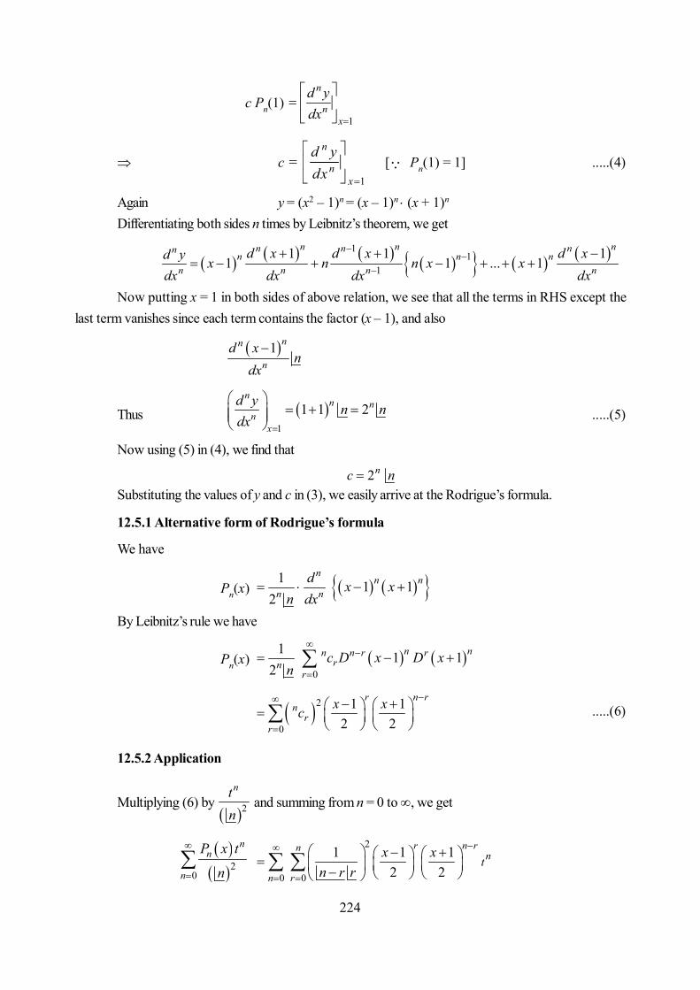
224
c Pn(1)1
n
nx
d ydx
c1
n
nx
d ydx
[ Pn(1) = 1] .....(4)
Again y = (x2 – 1)n = (x – 1)n (x + 1)n
Differentiating both sides n times by Leibnitz’s theorem, we get
11
11 1 1
1 1 ... 1n n nn n nn
n n nn n n n
d x d x d xd y x n n x xdx dx dx dx
Now putting x = 1 in both sides of above relation, we see that all the terms in RHS except thelast term vanishes since each term contains the factor (x – 1), and also
1 nn
nd x
ndx
Thus 1
1 1 2n
n nn
x
d y n ndx
.....(5)
Now using (5) in (4), we find that
2nc nSubstituting the values of y and c in (3), we easily arrive at the Rodrigue’s formula.
12.5.1 Alternative form of Rodrigue’s formula
We have
Pn(x) 1 1 12
nn n
n nd x x
n dx
By Leibnitz’s rule we have
Pn(x) 0
1 1 12
n nn n r rrn
rc D x D x
n
2
0
1 12 2
r n rn
rr
x xc
.....(6)
12.5.2 Application
Multiplying (6) by 2
ntn
and summing from n = 0 to , we get
20
nn
n
P x t
n
2
0 0
1 1 12 2
r n rn
n r
ntx x
n r r
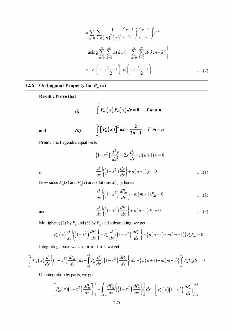
225
2 20 0
1 1 12 2
r nn r
n r
x x tn r
0 0 0 0
using , ,n
n k n kA k n A k n k
0 1 0 11 1;1; ;1;
2 2x xF t F t
.....(7)
12.6 Orthogonal Property for Pn (x)
Result : Prove that
(i) if1
1
0m nP x P x dx m n
and (ii) if1
2
1
22 1nP x dx m n
n
Proof. The Legendre equation is
2
221 2 1 0d y dyx x n n y
dxdx
or 21 1 0d dyx n n ydx dx
.....(1)
Now since Pm(x) and Pn(x) are solutions of (1), hence
21 1 0mm
dPd x m m Pdx dx
.....(2)
and 21 1 0nn
dPd x n n Pdx dx
.....(3)
Multiplying (2) by Pn and (3) by Pm and substracting, we get
2 21 1 1 1 0n mm n n m
dP dPd dP x x P x n n m m P Pdx dx dx dx
Integrating above w.r.t. x form –1to 1, we get
1 1
2 2
1 1
1 1n mm n
dP dPd dP x x dx P x dxdx dx dx dx
1
1
1 1 0n mn n m m P P dx
On integration by parts, we get
1 1
2 2
1 1
1 1n m nm
dP dP dPP x x x dxdx dx dx
12
11 m
ndPP x xdx
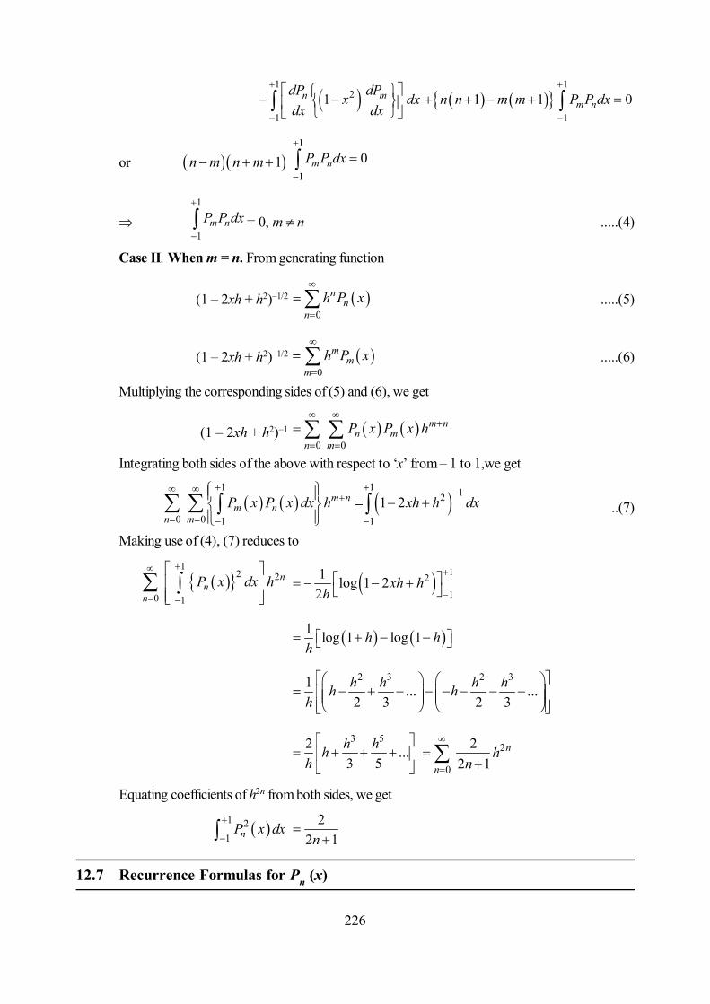
226
1
2
1
1n mdP dPx dxdx dx
1
1
1 1 0m nn n m m P P dx
or 1n m n m 1
1
0m nP P dx
1
1m nP P dx
= 0, m n .....(4)
Case II. When m = n. From generating function
(1 – 2xh + h2)–1/2 0
nn
nh P x
.....(5)
(1 – 2xh + h2)–1/2 0
mm
mh P x
.....(6)
Multiplying the corresponding sides of (5) and (6), we get
(1 – 2xh + h2)–1 0 0
m nn m
n mP x P x h
Integrating both sides of the above with respect to ‘x’ from – 1 to 1,we get
1 1 12
0 0 1 1
1 2m nm n
n mP x P x dx h xh h dx
..(7)
Making use of (4), (7) reduces to
1
2 2
0 1
nn
nP x dx h
12
1
1 log 1 22
xh hh
1 log 1 log 1h hh
2 3 2 31 ... ...2 3 2 3
h h h hh hh
3 52 ...3 5h hh
h
2
0
22 1
n
nh
n
Equating coefficients of h2n from both sides, we get
1 21 nP x dx
2
2 1n
12.7 Recurrence Formulas for Pn (x)

227
12.7.1 (n + 1) Pn + 1 (x) = (2n + 1) xPn(x) – nPn – 1(x), n 1,
or (2n + 1) xPn(x) = (n + 1) Pn + 1(x) + n Pn – 1(x)
Proof. We know that
(1 – 2xh + h2)–1/2 0
nn
nh P x
.....(1)
Differentiating (1) both sides w.r.t. h, we get
3 221 1 22
xh h
(– 2x + 2h) 1
0
nn
nnh P x
or (x – h) (1 – 2xh + h2)–1/2 = (1 – 2xh + h2) 1
0
nn
nnh P x
or (x – h) 0
nn
nh P x
= (1 – 2xh + h2) 1
0
nn
nnh P x
Equating coefficients of hn from both sides, we get
or xPn(x) – Pn – 1(x) = (n + 1) Pn + 1(x) – 2xn Pn(x) + (n – 1) Pn–1(x)
or (2n + 1) xPn(x) = (n + 1) Pn + 1(x) + nPn – 1(x)
12.7.2 1( ) ( ) ( )n n nnP x xP x P x
Proof.
Differentiating (1) w.r.t.’h’, we get
3 221 1 22
xh h
(– 2x + 2h) 1
0
nn
nnh P x
or (x – h) (1 – 2xh + h2)–3/2 1
0
nn
nnh P x
.....(2)
Again differentiating (1) w.r.t.’x’, we find that
3 221 1 22
xh h
× (–2h) 0
nn
nh P x
or h(1 – 2xh + h2)–3/2 '
0
nn
nh P x
Multiplying by (x – h) on both sides, we get
h(x – h) 3 221 2xh h
'
0
nn
nx h h P x

228
Using (2), we get 0
nn
nnh P x
'
0
nn
nx h h P x
Equating coefficients of hn from both sides of the above equation, we get' '
1( ) ( ) ( )n n nnP x xP x P x
12.7.3 (2n + 1) Pn(x) ' '1 1( ) ( )n nP x P x n
Proof. From recurrence formulas 12.7.1, we have(2n + 1) xPn(x) = (n + 1) Pn + 1(x) + nPn – 1(x)
Differentiating it w.r.t.’x’, we get(2n + 1) Pn(x) + (2n + 1) xPn(x) = (n + 1) Pn + 1(x) + nPn – 1(x) .....(3)
From recurrence 12.7.2, we havenPn(x) = xPn(x) – Pn – 1(x)
or ' ( )nxP x '1( ) ( )n nnP x P x .....(4)
Using (4) in (3), we get(2n + 1) Pn(x) + (2n + 1) [nPn(x) + Pn – 1(x)] = (n + 1)Pn + 1(x) + nPn – 1(x)
or (2n + 1) (n + 1) Pn(x) = (n + 1) Pn + 1(x) – (n + 1) Pn – 1(x)or (2n + 1) Pn(x) = P n + 1(x) – P n – 1(x)
12.7.4 (n + 1) Pn(x) = [P n + 1(x) – xP n(x)]
Proof. From recurrence formulae 12.7.2 and 12.7.3, we havenPn(x) = xP n(x) – P n – 1(x) .....(5)
(2n + 1) Pn(x) = P n + 1(x) – P n – 1(x) .....(6)Substracting, we get
(n + 1) Pn(x) = P n + 1(x) – xP n(x)
12.7.5 (1 – x2) P n(x) = x [Pn – 1(x) – xPn(x)]
Proof. From recurrence formulae 12.7.2, we havenPn(x) = xP n(x) – P n – 1(x)
Multiplying by x, we get nxPn(x) = x2P n(x) – xP n – 1(x) .....(7)Replacing n by (n – 1) in formula 12.7.4, we have
nPn–1(x) = P n(x) – xP n – 1(x) .....(8)Substracting (7) from (8), we have
x [Pn – 1(x) – xPn(x)] = (1 – x2)P n(x)
12.7.6 (1 – x2) P n(x) = (n + 1) [xPn(x) – Pn + 1(x)]
Proof. From recurrence formula 12.7.1, we have(2n + 1) xPn(x) = (n + 1) Pn + 1(x) + nPn – 1(x)
or (n + 1) xPn(x) + xnPn(x) = (n + 1) Pn + 1(x) + nPn – 1(x)
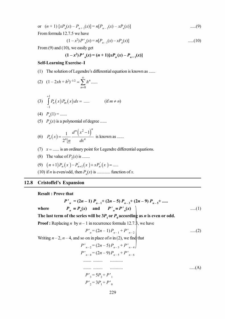
229
or (n + 1) [xPn(x) – Pn + 1(x)] = n[Pn – 1(x) – xPn(x)] .....(9)From formula 12.7.5 we have
(1 – x2) P n(x) = n[Pn – 1(x) – xPn(x)] .....(10)From (9) and (10), we easily get
(1 – x2) P n(x) = (n + 1)[xPn (x) – Pn + 1(x)]
Self-Learning Exercise–I
(1) The solution of Legendre’s differential equation is known as ......
(2) (1 – 2xh + h2)–1/2
0......n
nh
(3) 1
1n mP x P x dx
..... (if m n)
(4) Pn(1) = ......(5) Pn(x) is a polynomial of degree ......
(6) 2 11
2
nn
n n n
d xP x
n dx
is known as ......
(7) x = ...... is an ordinary point for Legendre differential equations.(8) The value of P2(x) is .......
(9) ' '11 .....n n nn P x P x xP x
(10) if n is even/odd, then Pn(x) is ............ function of x.
12.8 Cristoffel’s Expansion
Result : Prove thatP n = (2n – 1) Pn – 1+ (2n – 5) Pn – 3+ (2n – 9) Pn – 5+ .....
where Pn Pn(x) and P n P n(x) .....(1)The last term of the series will be 3P1 or P0 according as n is even or odd.Proof : Replacing n by n – 1 in recurrence formula 12.7.3, we have
P n = (2n – 1) Pn – 1 + P n – 2 .....(2)Writing n – 2, n – 4, and so on in place of n in (2), we find that
P n – 2 = (2n – 5) Pn – 3 + P n – 4
P n – 4 = (2n – 9) Pn – 5 + P n – 6
....... ........ ...........
....... ........ ........... .....(A)P 3 = 5P2 + P 1P 2 = 3P1 + P 0

230
When n is even, then adding the relations in (A) and (2), we get
P n = (2n – 1) Pn – 1+ (2n – 5) Pn – 3+ (2n – 9) Pn – 5+ .....+ 3P1 ( P 0(x) = 0)
and when n is odd, then
P n = (2n – 1) Pn – 1+ (2n – 5) Pn – 3+ (2n – 9) Pn – 5+ .....+ 5P2 + P0
( P 1= 1 = P0)
12.8.1 Cristoffel’s Summation Formula
Result : Prove that
0
2 1n
r rr
r P x P y
1 11 n n n nP x P y P y P xn
x y
.....(3)
Proof. Prom recurrence formula 12.7.1, we have(2r + 1) xPr (x) = (r + 1) Pr + 1 (x) + rPr – 1 (x) .....(4)
(2r + 1) yPr (y) = (r + 1) Pr + 1 (y) + rPr – 1 (y) .....(5)
Now multiplying (4) by Pr(y) and (5) by Pr(x) and subtracting, we find that
(2r + 1)(x – y) Pr (x) Pr (y) = (r + 1) [Pr + 1 (x) Pr (y) – Pr + 1 (y) Pr (x)]
+ r[Pr – 1 (x) Pr (y) – Pr (x) Pr – 1 (y)] .....(6)Taking r = 0, 1, 2 , .... n in (6) and adding the relations column-wise, we get the required result
(3).
12.9 Expression For Pn (cos ) in Terms of Cosine Series
we know that
(1 – 2xt + t2)–1/2 0
nn
nP x t
.....(1)
Taking x cos2
i ie e
in (1) we easily get
0
cos nn
nP t
= (1 – tei)–1/2(1 – te– i)–1/2 .....(2)
2 2 1 3..... 2 11 1 31 ... ...2 2 4 2 4 6.....2
i i n innte t e t e
n
2 2 1 3..... 2 11 1 31 ... ...2 2 4 2 4 6.....2
i i n innte t e t e
n
Now equating coefficients of t n both sides, we get
Pn(cos )
2 21 3 5.... 2 1 1 3 5.... 2 3 1
2 4 6.... 2 2 4 6... 2 2 2i n i nin inn n
e e e en n

231
4 41 3 5..... 2 5 1 3 .....2 4 6.... 2 4 2 4
i n i nne e
n
or Pn(cos ) = 1 3 5.... 2 1
1 4 6....2n
n
× 1 1 32cos 2cos 2 2cos 4 ...
2 1 2 1 2 3 1 2n nnn n n
n n n
the above formula is useful in obtaining the integrals involving the products of Pn(cos ) and sine andcosine multiple of .
Ex.1. Prove that 12 0
1 1
1n
n nn
z P P zzz xz z
Sol. We have RHS 10
nn n
nP P z
11
0 0
1n nn n
n nz P z P
z
.....(3)
Also1
10
nn
nz P
= zP1 + z2P2 + z3P3 + .. .....(4)
and0
nn
nz P
= P0 + zP1 + z2P2 + z3P3 + .. .....(5)
Substracting (5) from (4), we get
11
0
nn
nz P
0
0
nn
nz P P
.....(6)
Using (6) in (3), we get
RHS 00 0
1n nn n
n nz P z P P
z
0
0
11 nn
n
Pz P xz z
1 221 11 1 2xz zz z
0 1P
= L.H.S.Ex.2. Prove that Pn(1) = 1 and Pn(–1) = (–1)n
Sol. We have 0
nn
nh P x
= (1 – 2xh + h2)–1/2 .....(7)
For x = 1, we have
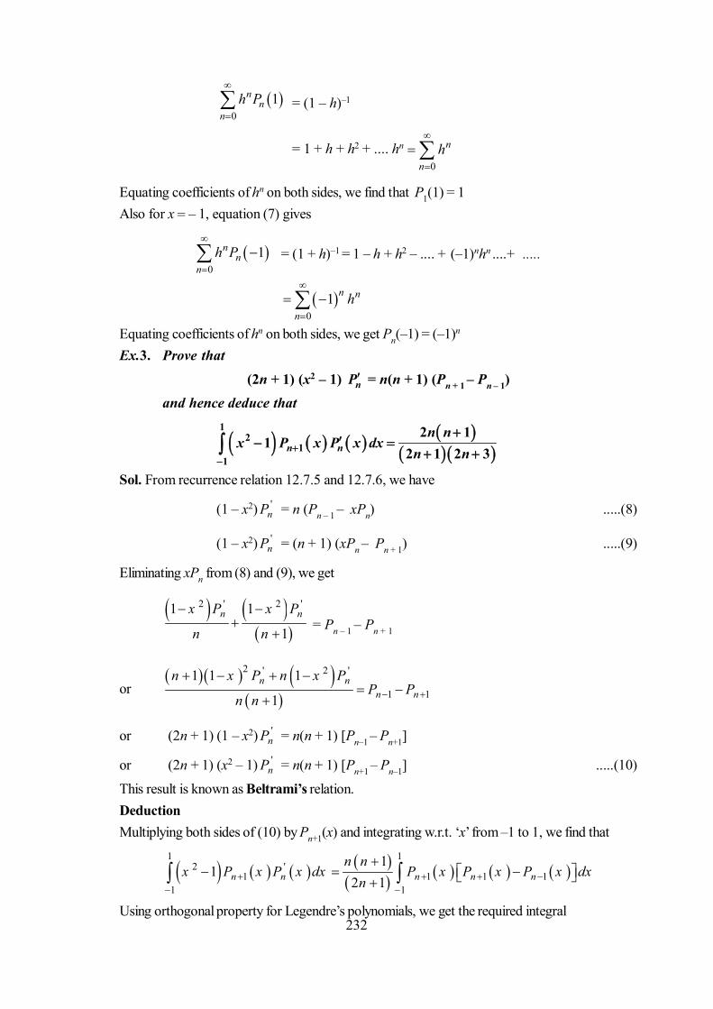
232
0
1nn
nh P
= (1 – h)–1
= 1 + h + h2 + .... hn
0
n
nh
Equating coefficients of hn on both sides, we find that P1(1) = 1Also for x = – 1, equation (7) gives
0
1nn
nh P
= (1 + h)–1 = 1 – h + h2 – .... + (–1)nhn ....+ .....
0
1 n n
nh
Equating coefficients of hn on both sides, we get Pn(–1) = (–1)n
Ex.3. Prove that
(2n + 1) (x2 – 1) nP = n(n + 1) (Pn + 1 – Pn – 1)and hence deduce that
12
11
2 11
2 1 2 3n nn n
x P x P x dxn n
Sol. From recurrence relation 12.7.5 and 12.7.6, we have
(1 – x2) 'nP = n (Pn – 1 – xPn) .....(8)
(1 – x2) 'nP = (n + 1) (xPn – Pn + 1) .....(9)
Eliminating xPn from (8) and (9), we get
2 ' 2 '1 1
1n nx P x P
n n
= Pn – 1 – Pn + 1
or
2 ' 2 '
1 1
1 1 1
1n n
n n
n x P n x PP P
n n
or (2n + 1) (1 – x2) 'nP = n(n + 1) [Pn–1 – Pn+1]
or (2n + 1) (x2 – 1) 'nP = n(n + 1) [Pn+1 – Pn–1] .....(10)
This result is known as Beltrami’s relation.DeductionMultiplying both sides of (10) by Pn+1(x) and integrating w.r.t. ‘x’ from –1 to 1, we find that
1 12 '
1 1 1 11 1
11
2 1n n n n nn n
x P x P x dx P x P x P x dxn
Using orthogonal property for Legendre’s polynomials, we get the required integral

233
Ex.4. Show that 2
0
1 1 cosn
nP x x x d
where n is a positive integer.This result is also known that Laplace’s first integral for Pn(x) .Proof. We know that
0 cosd
a b
2 2
,a b
we have a2 > b2 .....(11)
Taking a = 1 – hx and b = h 2 1x , thena2 – b2 = (1 – hx)2 – h2(x2 – 1) = 1 – 2xh + h2
Thus (11) becomes 22
0 1 21 1 cos
d
xh hhx h x
or (1 – 2xh + h2)–1/2
20
θ
1 1 cosθ
d
hx h x
or 0
π nn
nh P x
12
0
1 1 cosθ θh x x d
1
0
1 ht d
, where 2 1cost x x
2 2
0
1 ... ...n nht h t h t d
0 0
n n
nh t d
Equating coefficients of hn from both sides, we get
Pn(x)0
nt d
or Pn(x) 2
0
1 1cosn
x x d
Ex.5. Prove that
21 1
0
2 12 1 2 1 2 3n n
n nx P P dx
n n n
Proof. From Recurrence formulae 12.7.1 we have
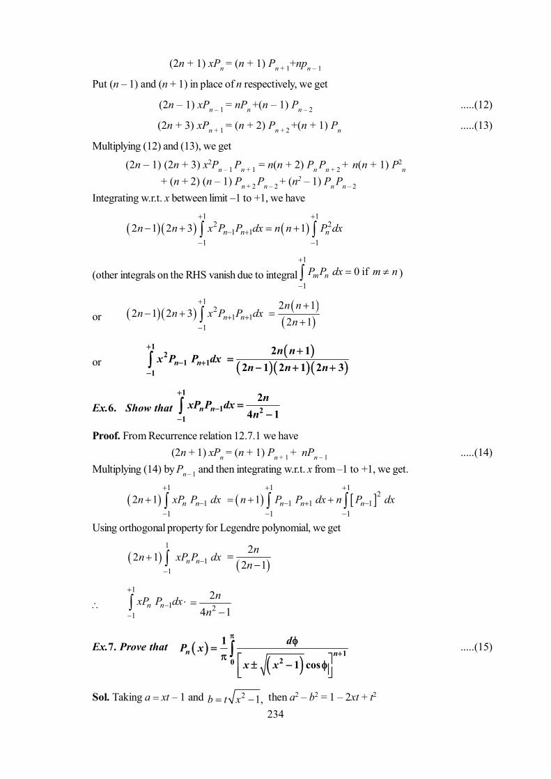
234
(2n + 1) xPn = (n + 1) Pn + 1+npn – 1
Put (n – 1) and (n + 1) in place of n respectively, we get
(2n – 1) xPn – 1 = nPn +(n – 1) Pn – 2 .....(12)
(2n + 3) xPn + 1 = (n + 2) Pn + 2 +(n + 1) Pn .....(13)
Multiplying (12) and (13), we get
(2n – 1) (2n + 3) x2Pn – 1 Pn + 1 = n(n + 2) Pn Pn + 2 + n(n + 1) P2n
+ (n + 2) (n – 1) Pn + 2 Pn – 2 + (n2 – 1) Pn Pn – 2
Integrating w.r.t. x between limit –1 to +1, we have
1 1
2 21 1
1 1
2 1 2 3 1n n nn n x P P dx n n P dx
(other integrals on the RHS vanish due to integral1
1
0 ifm nP P dx m n
)
or
12
1 11
2 12 1 2 3
2 1n nn n
n n x P P dxn
or1
21 1
1n nx P P dx
2 12 1 2 1 2 3
n nn n n
Ex.6. Show that 1
1 21
24 1n n
nxP P dxn
Proof. From Recurrence relation 12.7.1 we have(2n + 1) xPn = (n + 1) Pn + 1 + nPn – 1 .....(14)
Multiplying (14) by Pn – 1 and then integrating w.r.t. x from –1 to +1, we get.
1
11
2 1 n nn xP P dx
1 1
21 1 1
1 1
1 n n nn P P dx n P dx
Using orthogonal property for Legendre polynomial, we get
1
11
2 1 n nn xP P dx
2
2 1n
n
1
11
n nxP P dx
22
4 1n
n
Ex.7. Prove that
120
1
1 cosn n
dP x
x x
.....(15)
Sol. Taking a = xt – 1 and 2 1,b t x then a2 – b2 = 1 – 2xt + t2
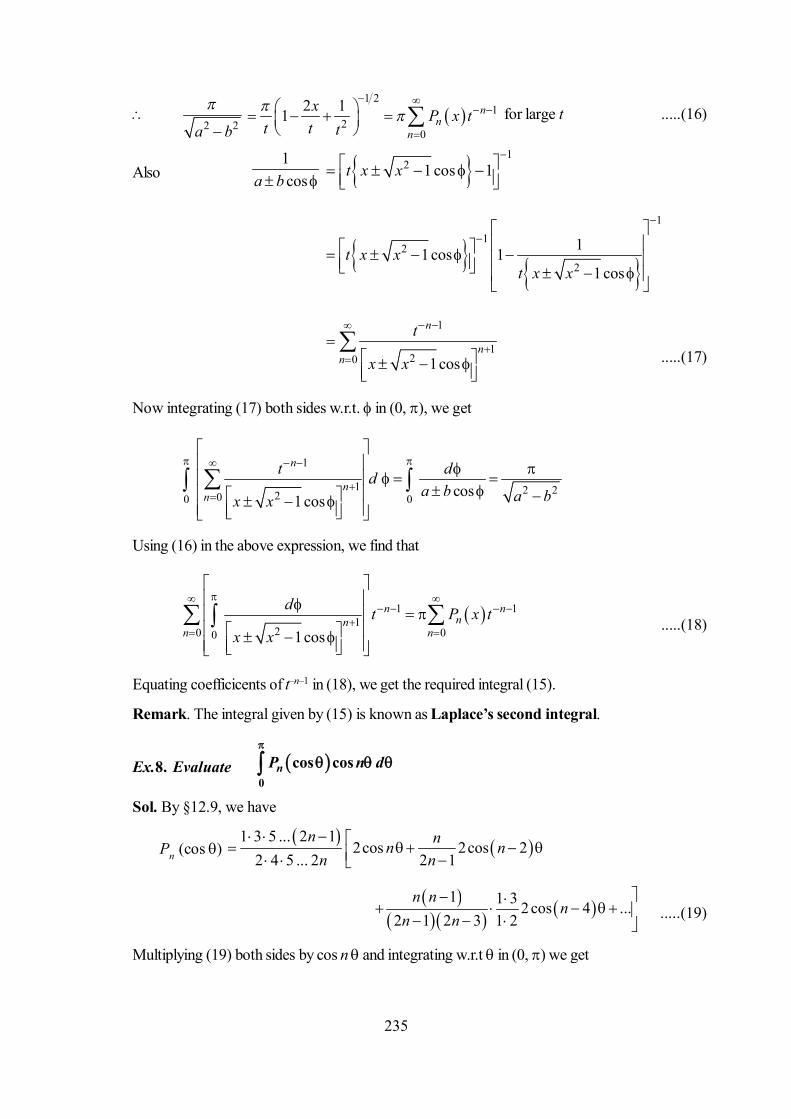
235
2 2a b
1 21
20
2 11 nn
n
x P x tt t t
for large t .....(16)
Also1cosa b 1
2 1 cos 1t x x
11
22
11cos 11cos
t x xt x x
1
120 1cos
n
nn
t
x x
.....(17)
Now integrating (17) both sides w.r.t. in (0, ), we get
1
1 2 2200 0 cos1cos
n
nn
t dda b a bx x
Using (16) in the above expression, we find that
1 11
20 00 1cos
n nnn
n n
d t P x tx x
.....(18)
Equating coefficicents of t–n–1 in (18), we get the required integral (15).
Remark. The integral given by (15) is known as Laplace’s second integral.
Ex.8. Evaluate 0
cos cosnP n d
Sol. By §12.9, we have
Pn (cos ) 1 3 5 ... 2 1
2cos 2cos 22 4 5 ... 2 2 1
n nn nn n
1 1 3 2 cos 4 ...2 1 2 3 1 2
n nn
n n
.....(19)
Multiplying (19) both sides by cos n and integrating w.r.t in (0, ) we get
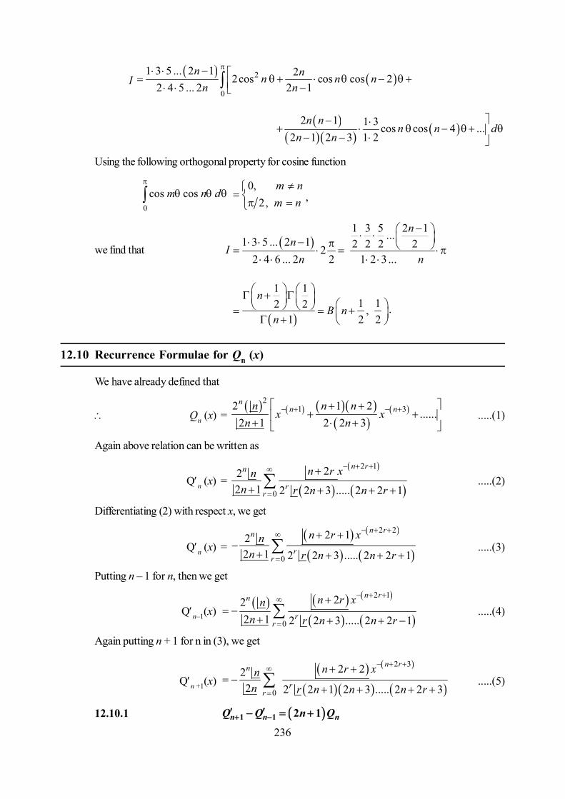
236
I 2
0
1 3 5 ... 2 1 22cos cos cos 22 4 5 ... 2 2 1
n nn n nn n
2 1 1 3 cos cos 4 ...2 1 2 3 1 2
n nn n d
n n
Using the following orthogonal property for cosine function
0
cos cosm n d
0,
2,m nm n
,
we find that I 1 3 5 2 1...1 3 5 ... 2 1 2 2 2 22
2 4 6 ... 2 2 1 2 3 ...
nn
n n
1 11 12 2 ,
1 2 2
nB n
n
.
12.10 Recurrence Formulae for Qn (x)
We have already defined that
Qn (x) =
21 32 1 2
......2 1 2 2 3
nn nn n n
x xn n
.....(1)
Again above relation can be written as
Qn (x) =
2 1
0
222 1 2 2 3 ..... 2 2 1
n rn
rr
n r xnn r n n r
.....(2)
Differentiating (2) with respect x, we get
Qn (x) =
2 2
0
2 122 1 2 2 3 ..... 2 2 1
n rn
rr
n r xnn r n n r
.....(3)
Putting n – 1 for n, then we get
Qn–1(x)
2 1
0
222 1 2 2 3 ..... 2 2 1
n rn
rr
n r xnn r n n r
.....(4)
Again putting n + 1 for n in (3), we get
Qn +1(x)
2 3
0
2 222 2 2 1 2 3 ..... 2 2 3
n rn
rr
n r xnn r n n n r
.....(5)
12.10.1 1 1 2 1n n nQ Q n Q

237
Proof. Using (1) and (4) above, we get
Qn –1+(2n + 1) Qn = –
2 1
0
2 22 1 2 2 3 ...... 2 2 1
n rn
rr
n n r xn r n n r
2 1
0
2 22 12 1 2 2 3 ..... 2 2 1
n rn
rr
n n r xnn r n n r
2 1
0
2 2 2 2 1 2 12 1 2 2 3 .... 2 2 1
n rn
rr
n n r x n r nn r n n r
2 1
0
2 2 22 1 2 2 3 ....... 2 2 1
n rn
rr
n n r x rn r n n r
2 1
11
2 22 1 2 1 2 3 ...... 2 2 1
n rn
rr
n n r xn r n n r
Putting r – 1 = s r = s + 1, therefore
Qn –1+(2n + 1) Qn
2 3
0
2 2 22 1 2 2 3 ...... 2 2 3
n sn
sr
n n s xn s n n s
'1nQ x LHS
12.10.2 1 11 2 1n n nnQ n Q n x Q
Proof. Using (1) and (4) above, we get
(2n + 1)x Qn– (n + 1) Qn-1
2 2
0
2 2 12 12 1 2 2 3 ...... 2 2 1
n rn
rr
n n r xn xn r n n r
2 1
0
2 212 1 2 2 3 ...... 2 2 1
n rn
rr
n n r xnn r n n r
2 1
0
1 2 22 1 2 2 3 ...... 2 2 1
n n r
rr
n n r xn r n n r
12 1 2 1 1 2 2 1n x n r x n n r
2 1
0
1 2 2 1 22 1 2 2 3 ....... 2 2 1
n n r
rr
n n r x nrn r n n r
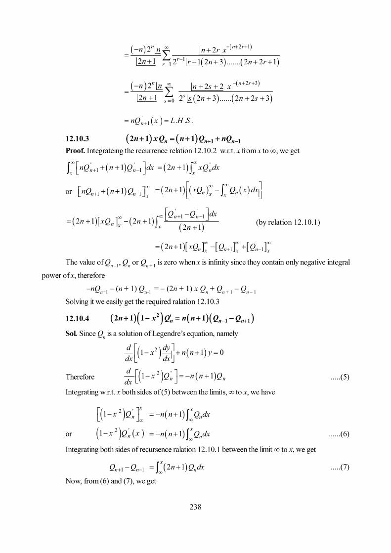
238
2 1
11
2 22 1 2 1 2 3 ....... 2 2 1
n n r
rr
n n n r xn r n n r
2 3
0
2 2 22 1 2 2 3 ...... 2 2 3
n n s
ss
n n n s xn s n n s
'1 . . .nnQ x L H S
12.10.3 n n nn x Q n Q nQ1 12 1 1 Proof. Integrateing the recurrence relation 12.10.2 w.r.t. x from x to , we get
' '1 11n nx
nQ n Q dx
'2 1 nxn xQ dx
or 1 11n n xnQ n Q
2 1 n nx xn xQ Q x dx
' '1 1
2 1 2 12 1
n nn x x
Q Q dxn xQ n
n
(by relation 12.10.1)
1 12 1 n n nx x xn xQ Q Q
The value of Qn –1, Qn or Qn + 1 is zero when x is infinity since they contain only negative integral
power of x, therefore
–nQn+1 – (n + 1) Qn–1 = – (2n + 1) x Qn + Qn + 1 – Qn – 1
Solving it we easily get the required ralation 12.10.3
12.10.4 n n nn x Q n n Q Q21 12 1 1 1
Sol. Since Qn is a solution of Legendre’s equation, namely
21 1 0d dyx n n ydx dx
Therefore 2 '1 1n nd x Q n n Qdx
.....(5)
Integrating w.r.t. x both sides of (5) between the limits, to x, we have
2 '1x
nx Q
1x
nn n Q dx
or 2 '1 nx Q x 1
xnn n Q dx
......(6)
Integrating both sides of recursence ralation 12.10.1 between the limit to x, we get
1 1n nQ Q 2 1x
nn Q dx
.....(7)
Now, from (6) and (7), we get

239
2 '1 nx Q x
1 112 1
n nQ x Q xn n
n
2 '2 1 1 nn x Q x 1 11 n nn n Q x Q x
12.11 Cristoffel’s Second Summation Formula
Result. n
r rr
y x r P x Q y1
2 1
n n n nn P x Q y P x Q y1 11 1 ......(1)
Proof : From recurrence formulas for Pn(x) and Qn(x), we have
(2n + 1) x Pn (x) 1 11 n nn P x nP x .....(2)
(2n + 1) y Qn (y) 1 11 n nn Q y nQ y .....(3)Multiplying (2) by Qn (y) and (3) by Pn(x) and subtracting, we have(2n + 1 ) (x – y) Pn (x) Qn (y) + n {Pn–1 (x) Qn–1 (y) – Qn-1 (y)Pn (x)}
1 11 n n n nn P x Q y P x Q y .....(4)Taking n = 1, 2, 3 ...... , n in (4) and adding, we get
1 0 0 11
2 1n
r rr
y x r P x Q y Q x P y Q y P x
1 11 n n n nn P x Q y P x Q y .....(5)
Now since Q1 (y) = y, Q0 (y) = 1, P1 (x) = x, P0 (x) = 1, therefore (5) gives the requiredresult (1).
12.12 Relations Between Pn (x) and Qn (x)
Result. Prove that y x1
m mm
m P x Q y0
2 1
and hence deduce that
Qm (y)= mP x
dx yy x
1
1, 1
Proof : Let f (x) = 1
1 1 1 xy x y y
21 1 ..... ......
m
mx x xyy y y
1 2 2 3 1...... .......m my x y x y x y
20 1 2 .......A A x A x (Suppose that) ......(1)
where A’s are constants.

240
Further suppose that f (x) = 0
,m mm
B P x
then we know that Bm=
21 21.2.3....... ......
1.3.5...... 2 1 2 2 3m mm mm A A
m m
......(2)
Comparing (1) and (3) we get
A0 = 11 21, , ...., ,.....m
my A y A y
B m =
1 31 2! ......
1 3 5 2 1 2 2 3m mm mm y y
m m
= (2m + 1) Qm (y)
Hence1
y x
02 1 m m
mm Q y P x
.....(3)
Now multiplying (3) by Pm (x) and integrating w.r.t x in the interval (–1, 1), we find that
1
1
1mP x dx
y x
1
10
2 1m m mm
P x m P x Q y dx
1 2
12 1m mQ y P x m dx
1
1( ) 0,nPm n P x dx m n
22 12 1nQ y m
m
1 21
22 1m nP x d
m
1
1
1 12 m nP x dx Q y
y x
This integral is called the Neumann’s integral for Qn (y).
Ex.1. Prove that n n n nx Q P P Q c2 1 and deduce that
(i)
nxn n
Q dxP x P2 21
(ii) xQ xx0
1 1log2 1
(iii) x xQ xx0
1log 12 1
Sol. The Legendre’s equation is
2
221 2 1 0d y dyx x n n y
dxdx
Since Pn (x) and Qn (x) are both the solution of this equation, therefore
2
221 2 1 0n n
nd P x dP x
x x n n P xdxdx
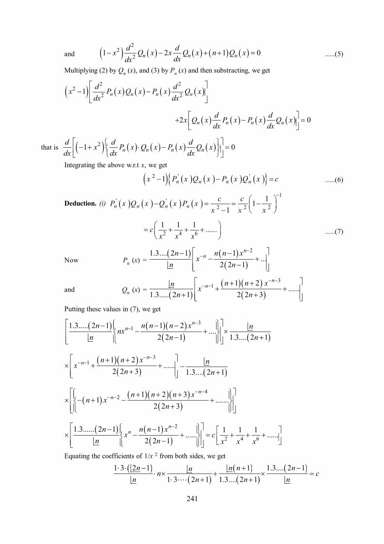
241
and 2
221 2 1 0n n n
d dx Q x x Q x n Q xdxdx
.....(5)
Multiplying (2) by Qn (x), and (3) by Pn (x) and then substracting, we get
2 2
22 21 n n n n
d dx P x Q x P x Q xdx dx
2 0n n n nd dx Q x P x P x Q xdx dx
that is 21 0n n n nd d dx P x Q x P x Q xdx dx dx
Integrating the above w.r.t x, we get
2 ' '1 n n n nx P x Q x P x Q x c .....(6)
Deduction. (i) 1
' '2 2 2
111n n n n
c cP x Q x Q x P xx x x
2 4 61 1 1 ......cx x x
.....(7)
Now Pn (x) =
21.3.... 2 1 1...
2 2 1
nnn n n x
xn n
and Qn (x) =
31 1 2
......1.3..... 2 1 2 2 3
nn n n xn x
n n
Putting these values in (7), we get
311.3..... 2 1 1 2
....2 2 1 1.3.... 2 1
nnn n n n x nnx
n n n
31 1 2
......2 2 3
nn n n x
xn
1.3.... 2 1
nn
42 1 2 3
1 .......2 2 3
nn n n n x
n xn
2
2 4 61.3...... 2 1 1 1 1 1...... ......
2 2 1
nnn n n x
x cn n x x x
Equating the coefficients of 1/x 2 from both sides, we get
1 3 2 1 1 1.3.... 2 11 3 2 1 1.3.... 2 1
n n n nnn cn n n n
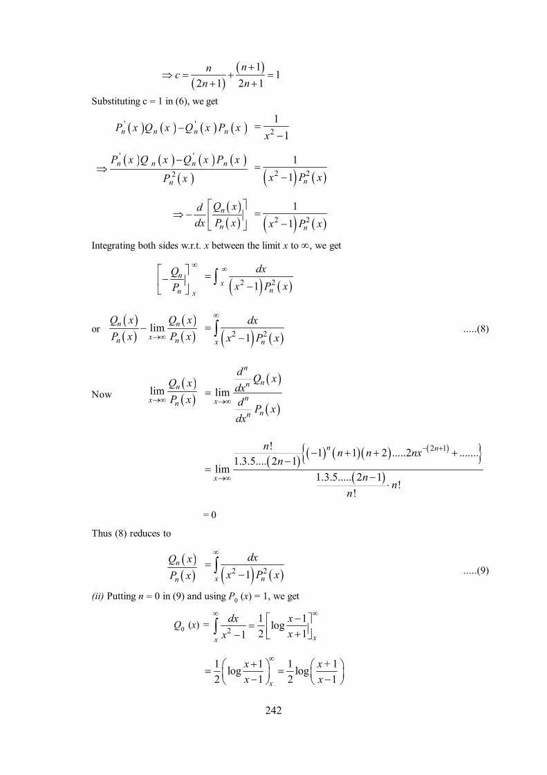
242
1
12 1 2 1
nncn n
Substituting c = 1 in (6), we get
' 'n n n nP x Q x Q x P x 2
11x
' '
2n n n n
n
P x Q x Q x P x
P x
2 2
11 nx P x
n
n
Q xddx P x
2 21
1 nx P x
Integrating both sides w.r.t. x between the limit x to , we get
n
n x
QP
2 21x
n
dxx P x
or
limn nxn n
Q x Q xP x P x
2 21 nx
dxx P x
.....(8)
Now
lim nx n
Q xP x
lim
n
nn
nxnn
d Q xdxd P xdx
2 1! 1 1 2 .....2 .......1.3.5.... 2 1
lim1.3.5..... 2 1
!!
n n
x
n n n nxn
nn
n
= 0
Thus (8) reduces to
n
n
Q xP x 2 21 nx
dxx P x
.....(9)
(ii) Putting n = 0 in (9) and using P0 (x) = 1, we get
Q0 (x) = 2
1 1log2 11 xx
dx xxx
1 1 1 1log log2 1 2 1x
x x +x x
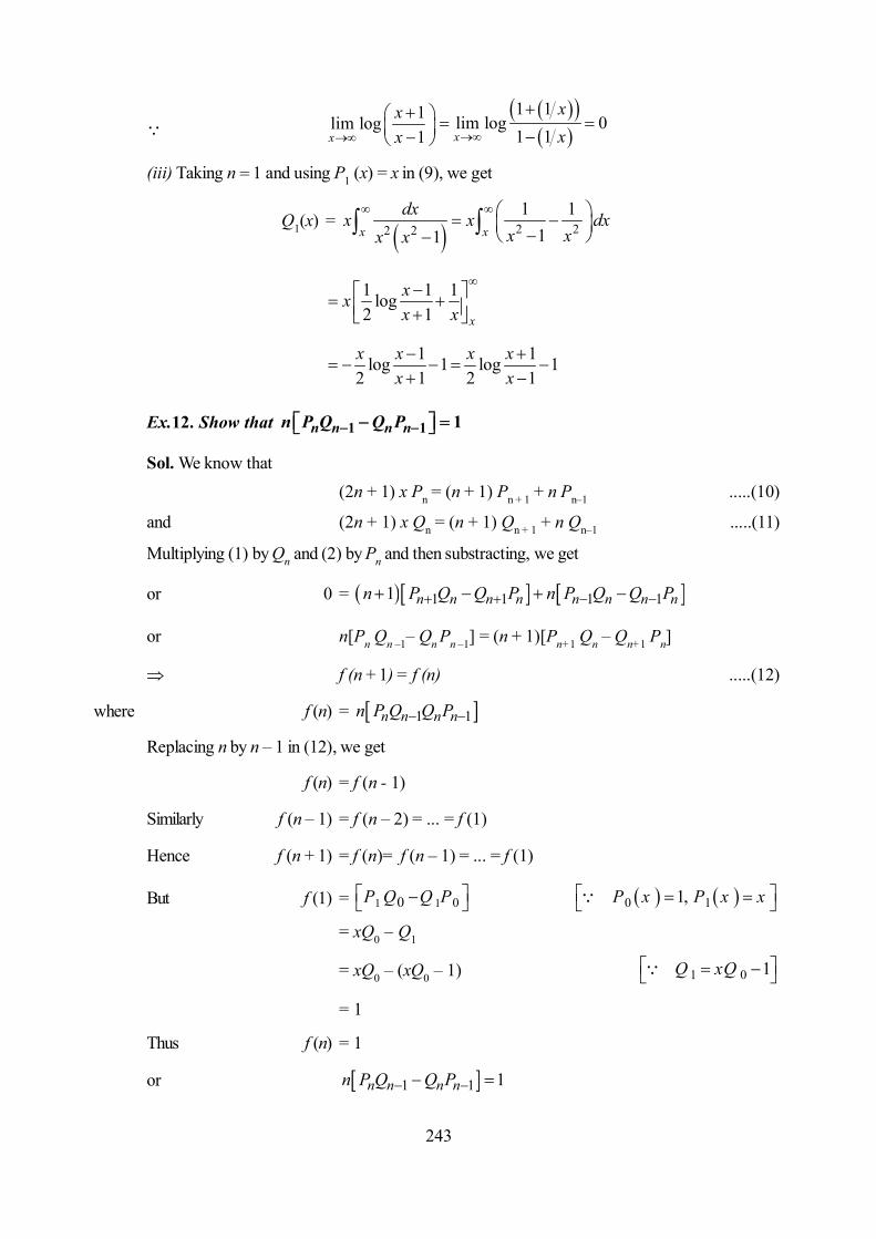
243
1lim log1x
xx
1 1lim log 0
1 1x
xx
(iii) Taking n = 1 and using P1 (x) = x in (9), we get
Q1(x) = 2 22 2
1 111x x
dxx x dxx xx x
1 1 1log2 1 x
xxx x
1 1log 1 log 12 1 2 1x x x x
x x
Ex.12. Show that n n n nn P Q Q P1 1 1
Sol. We know that(2n + 1) x Pn = (n + 1) Pn + 1 + n Pn–1 .....(10)
and (2n + 1) x Qn = (n + 1) Qn + 1 + n Qn–1 .....(11)
Multiplying (1) by Qn and (2) by Pn and then substracting, we get
or 0 = 1 1 1 11 n n n n n n n nn P Q Q P n P Q Q P
or n[Pn Qn –1– Qn Pn –1] = (n + 1)[Pn+1 Qn – Qn+1 Pn]
f (n + 1) = f (n) .....(12)
where f (n) = 1 1n n n nn P Q Q P
Replacing n by n – 1 in (12), we get
f (n) = f (n - 1)
Similarly f (n – 1) = f (n – 2) = ... = f (1)
Hence f (n + 1) = f (n)= f (n – 1) = ... = f (1)
But f (1) = 1 1 00P Q Q P 0 11,P x P x x
= xQ0 – Q1
= xQ0 – (xQ0 – 1) 1 0 1Q xQ
= 1
Thus f (n) = 1
or 1 1 1n n n nn P Q Q P

244
Self – Learning Exercise–II
1. 21 ........ndQd xdx dx
2. ' '1 1 ...........n nQ Q
3. Legendre’s function of second kind is ...........
12.13 Summary
In this unit we studied the Legendre’s differential equation and its solution as Legendre function
of first and second kinds. We also studied the recurrence relation, generating function, orthogo-
nal property, Rodrigues formulae and other important formulas for these functions.
12.14 Answers to Self Learning Exercises
Exercise - I
1. Legendre function of first kind 2. Pn (x)
3. 0 4. 1
5. n 6. Rodrigues formulae
7. 0 8. 21 5 32
x x
9. 0 10. Even / odd
Exercise - II
1. – n (n + 1) Qn (x) 2. (2n + 1) Qn (x)
3. Qn (x)
12.15 Exercise
1. Prove that Pn (– x) = (– 1)n Pn (x) and Pn (– 1) = (– 1)n.
2. Express P (x) = x4 + 2x3 + 2x2 – x – 3 in terms of Legendre’s polynomial
[Ans : 4 3 2 18 4 40 1 22435 5 21 5 105 oP x P x P x P x p x P x ]
3. Show that 1
10nP x dx
except when n = 0 in which case the value of integral is 2.
4. Prove that
1 22 '
1
2 11
2 1nn n
x P x dxn

245
5. Show that Pn (x) Qn–2 (x) – Qn (x)Pn–2 (x) = 2 1
1n
xn n
6. Prove that ' '1n n nxQ Q nQ
7. Prove that
2 21
1 0 20
111 ; ;2 1
nn
n
t xP x t xt F
xt
8. Prove that
2 1 21 1, ; 1 ; 1
2 2 2n
nn nP x x F
x
9. Show that
2 2
0 10
1; 1 ;
! 4
nn xt
n
t xP x te F
n
10. Find the values of P2n+1(0), P2n (0), P2n (0) and P2n+1 (0)
[Ans. 1 1/ 2 1 3 / 2
0, , 0 ,! !
n nn n
n n
]
11. Establish the Murphy’s formula
2 11, 1 ; 1 ;
2nxP x F n n
and deduce that
(a) 2 111 , 1 ; 1 ;
2n
nxP x F n n
(b) 2 11 1, ; 1 ;
2 1
n
nx xP x F n n
x
(c) 2 11 1, ;1;
2 1
n
nx xP x F n n
x
(d) 22 1cos , 1 ; 1 ; sin / 2nP F n n
12. Prove that
2 1 22 1/ 2 1 1 1, ; ;
! 2 2 2 2
n nn
nx n nP x F n
n x
13. Prove that

246
20
01
!
nn xt
n
P x te J t x
n
14. Prove that
'2 42 3 2 7 .......n n n nxP nP n P n P
and hence or other wise show that
(a)1 '1
22 1n n
nxP P dxn
(b) 1 '1
0n mxP P dx
or 2
2 1n
n
15. Show that 1 21 1n
nP x dxn
16. Show that
1 211
1 1
2 1 2 1 2
n
n n
nP x dx
n n
17. Prove that
11
0nP x dx
, n 0 and 101
2P x dx
18. Prove that
2 2 22 2 2 2 20 13 ...... 2 1 1 1n n nP P n P n P x P

247
Unit 13 : Bessel’s FunctionsStructure of the Unit
13.0 Objective
13.1 Introduction
13.2 Definition
13.3 Bessel’s Equation and its solution
13.4 Relation between Jn (x) and J– n(x)
13.5 Generating function
13.6 Recurrence Formulae
13.7 Addition Theorem
13.8 Orthogonal Property
13.9 Integral Representation of Bessel Functions
13.10 An Important Integral
13.11 Summary
13.12 Answers to Self-Learning Exercise
13.13 Exercise
13.0 Objective
In this unit you will learn about Bessel function which besides the solution of the well-known
Bessel’s equation may also be introduced through a generating function. You will also study important
properties for this function.
13.1 Introduction
No other special function have received such detailed treatment in readily available treatises as
have the Bessel functions. These functions were first introduced by F.W. Bessel, who is regarded as the
founder of the modern practical Astronomy. In fact several problems of mathematical physics lead to
Laplace’s equation and in turn converts into Bessel’s equation when there is a cylindrical symmetry. There-
fore Bessel’s function and Bessel’s equation have received great attention.
In this unit, we introduce the Bessel function through the Bessel’s differential equation and gener-

248
ating function. We then discuss the important properties (such as Recurrence formulae, orthogonal property,
Addition theorem, integral representations etc.) for this function.
13.2 Definition
13.2.1 Bessel Differential Equation
The differential equation
2
2 2 22 0dyd yx x x n y
dxdx .....(1)
is called Bessel’s differential equation of order n where n is non-negative real number.
13.2.2 Bessel’s function of the first kind of order n
It denoted by Jn(x) and is defined as
2
0
1! 1 2
r n r
nr
xJ xr n r
.....(2)
(where n is any non-negative constant)
2
0 12
; 1;1 4
nx xF nn
.....(3)
It n is a negative integer, then we put
1 nn nJ x J x .....(4)
1 nn nJ x J x .....(5)
Equations (3) and (4) together define Jn (x) for all finite x and n.Replacing n by 0 and 1 in (2), we find that
2 4 6
0 2 2 4 4 4 2...1
2 2 4 2 4 6x x xJ x .....(6)
and 3 5
1 2 2 2...
2 2 3 2 4 6x x xJ x
......(7)
13.3 Bessel’s Equation and its Solution
Bessel differential equation is
2
2 2 22 0d y dyx x x n
dxdx .....(1)
The equation (1) has a regular singular point at x = 0, and an irregular singular point at x = ,while all other points are ordinary points. The solution of equation (1) called Bessel’s function will de-pend upon n. This index n may be non-integer, a positive integer or zero. We discuss three possibilities :
Case I. Solution of (1) for non-integral values of n
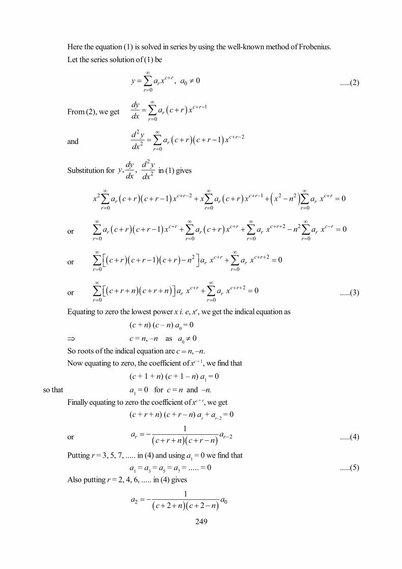
249
Here the equation (1) is solved in series by using the well-known method of Frobenius.Let the series solution of (1) be
00
, 0c rr
ry a x a
.....(2)
From (2), we get 1
0
c rr
r
dy a c r xdx
and 2
22
01 c r
rr
d y a c r c r xdx
Substitution for 2
2, ,dy d yydx dx
in (1) gives
2 2 1 2 2
0 0 01 0c r c r c r
r r rr r r
x a c r c r x x a c r x x n a x
or 2 2
0 0 0 01 0c r c r c r c r
r r r rr r r r
a c r c r x a c r x a x n a x
or 2 2
0 01 0c r c r
r rr r
c r c r c r n a x a x
or 2
0 00c r c r
r rr r
c r n c r n a x a x
.....(3)
Equating to zero the lowest power x i. e, xr, we get the indical equation as(c + n) (c – n) a0 = 0
c = n, –n as a0 0So roots of the indical equation are c = n, –n.Now equating to zero, the coefficient of xc + 1, we find that
(c + 1 + n) (c + 1 – n) a1 = 0
so that a1 = 0 for c = n and –n.Finally equating to zero the coefficient of xc + r, we get
(c + r + n) (c + r – n) ar + ar–2 = 0
or 21
r ra ac r n c r n .....(4)
Putting r = 3, 5, 7, ..... in (4) and using a1 = 0 we find thata1 = a3 = a5 = a7 = ..... = 0 .....(5)
Also putting r = 2, 4, 6, ..... in (4) gives
2 01
2 2a a
c n c n

250
4 01 and so on
2 2 4 4a a
c n c n c n c n
.
Putting these values in (2), we get
2 40 2 4 1 3 5
0..... as 0c r c c c
rr
y a x a x a x a x a a a
or 2 4
0 ....12 2 2 2 4 4
c x xy a xc n c n c n c n c n c n
Replacing c by n and – n, we get
2 4
0 1 .....2 2 2 2 4 2 2 2 4
n x xy a xn n n
.....(5)
and 2 4
0 1 .....2 2 2 2 2 2 4 2 4
n x xy a xn n n
.....(6)
The particular solution of the equation (1) obtained from (5) above by taking the arbitrary con-
stant 01
2 1nan
is called the Bessel function of the first kind of order n. It will be denoted by
Jn (x). Thus we have
2 41 .....
4 1 4 8 1 22 1
n
n nx x xJ x
n n nn
.....(7)
or
2
0
11 2
rn r
nr
xJ x xr n r
.....(8)
Similarly taking 01
2 1nan
in (6), we get
2
0
11 2
r r n
nr
xJ xr n r
.....(9)
Let n be non-integral. Since n is not an integer and r is always integral, the factor (–n + r + 1)in (9) is always finite and non-zero (m) is always finite for m 0 or a negative integer.) Again for2r < n, (9) shows that J–n(x) contains negative powers of x. On the other hand, (8) shows that Jn(x)does not contain negative power of x at all. Therefore for x = 0, Jn(x) is finite. While J–n(x) is infinite, andso one can not be expressed as constant multiple of the other. Thus we conclude that Jn(x) and J–n(x)are independent solutions of (1) when n is not an integer. Thus general solution of Bessel’s equation (1)when n is not an integer is
y = AJn(x) + BJ–n(x)where A and B one arbitrary constants.
Case-II. Solution for positive integral values of n and for n = 0.It n is a positive integer, then for c = –n, the recurrence relation (4) gives

251
21
2r ra ar n r
which breaks when r = 2n.Also if n = 0, the two roots of the indical equation becomes equal and in that case the afore-
mentioned method is not applicable.In both the cases, the second solution of (1) can be found by using methods mentioned in unit 9.
13.4 Relation between Jn(x) and J–n(x), n being an integer
Result. 1 nn nJ x J x .....(1)
Proof. We consider two cases :Case I. Let n be a positive integer
We have
2
0
11 2
r r n
nr
xJ xr n r
.....(2)
Since n > 0, so (–n + r + 1) is infinite. for r = 0, 1, ..., n – 1, therefore (2) becomes
211 2
r r n
nr n
xJ xr n r
2
0
11 2
m n m n
m
xm n m
(taking r = m + n)
2
0
11
1 2
r n rn
r
xr r n
1 nnJ x (by definition)
Case II. Let n < 0.Putting n = –p, where p is a tive integerSince P > 0, therefore form Case I, we have
1 pp pJ x J x
or 1 pp pJ x J x
Putting p = –n, we get the required result.Hence the relation (1) is true for any integer.
13.5 Generating Function
Theorem. Prove that when n is a positive integer Jn (x) is the coefficient of zn in the
expansion of 1exp x z
z z
in ascending and decending power of z.

252
Proof. We have1exp exp exp
2 2x xz xzz z z
2 12 11 .... ....
2 2 2 2 2 1
n nn nx x z x z x zzn n
12 12
11 1 11 .... ....
2 2 2 2 2 1
n nn nnnzx x z x xz z
n n
....(1)
Multiplying the R.H.S. of (1) term by term, we find that coefficient of zn is2 41 1 1 ....
2 1 2 2 2 2
x n nx x xn n n
2
0
11 2
r n r
nr
x J xr n r
.....(2)
Similarly the coefficient of z–n in the expansion (1) is
1 22 41 1 1
.... 12 1 2 2 2 2
n n nn n nn
nx x x J x
n n n
.....(3)
Further, the term independent of z is
2 4
02 2 21 ....2 2 4x x J x
.....(4)
Hence relation (1) with help of (2), (3) and (4) may be written as
20 1 22
1 1 1exp ....2x z J x z J x z J x
z z z
Since J–n(x) = (–1)n Jn(x), therefore
1exp2
nn
n
x z J x zz
.....(5)
13.6 Recurrence Formulae for Jn (x)
13.6.1 xJn (x) = nJn (x) – xJn + 1 (x)
Proof. We have
nJ x
2
0
11 2
r n r
r
xr n r
Differentiating above w.r.t. x, we get
nJ x
2 1
0
1 2 11 2 2
r n r
r
n r xr n r
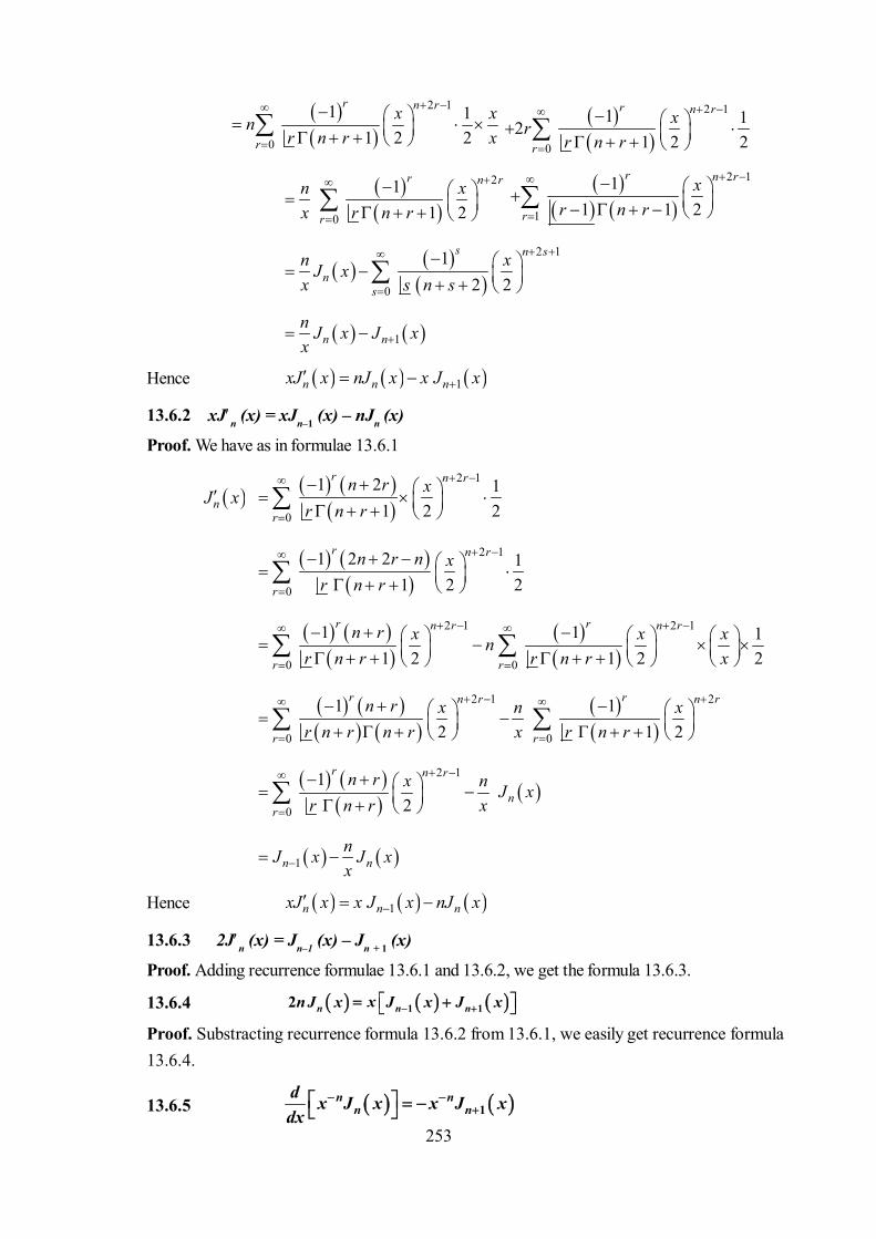
253
2 1
0
1 11 2 2
r n r
r
x xnr n r x
2 1
0
1 121 2 2
r n r
r
xrr n r
2
0
11 2
r n r
r
n xx r n r
2 1
1
11 1 2
r n r
r
xr n r
2 1
0
12 2
s n s
ns
n xJ xx s n s
1n nn J x J xx
Hence 1n n nxJ x nJ x x J x
13.6.2 xJn (x) = xJn–1 (x) – nJn (x)
Proof. We have as in formulae 13.6.1
nJ x
2 1
0
1 2 11 2 2
r n r
r
n r xr n r
2 1
0
1 2 2 11 2 2
r n r
r
n r n xr n r
2 1 2 1
0 0
1 1 11 2 1 2 2
r rn r n r
r r
n r x x xnr n r r n r x
2 1 2
0 0
1 12 1 2
r rn r n r
r r
n r x n xr n r n r x r n r
2 1
0
12
r n r
nr
n r x n J xr n r x
1n nnJ x J xx
Hence 1n n nxJ x x J x nJ x
13.6.3 2Jn (x) = Jn–1 (x) – Jn + 1 (x)
Proof. Adding recurrence formulae 13.6.1 and 13.6.2, we get the formula 13.6.3.
13.6.4 1 12 n n nxn J x J x J x
Proof. Substracting recurrence formula 13.6.2 from 13.6.1, we easily get recurrence formula13.6.4.
13.6.5 1n n
n nd x J x x J xdx

254
Proof. By formulas 13.6.1, we have
1n n nx J x n J x x J x
Multiplying both sides of above by x – n–1, we have
11
n n nn n nx J x nx J x x J x
or 11
n n nn n nx J x nx J x x J x
or 1n n
n nd x J x x J xdx
13.6.6 1n n
n nd x J x x J xdx
Proof. By formula 13.6.2, we have
1n n nx J x x J x n J x
Multiplying both sides of above by x n–1, we have
11
n n nn n nx J x x J x nx J x
or 11
n n nn n nx J x nx J x x J x
or 1n n
n nd x J x x J xdx
Ex.1. Prove that 1 22 sinJ x xx
Sol. We know that
2 41 ...........
2 2 2 2 4 2 2 2 42 1
n
n nx x xJ x
n n nn
Puting 12
n and using 32 2
, we get
2 4
1 22 1 ...
2 3 3 5 2 4x x xJ x
3 52 ...
31 51x xx
x
2 sin xx
Ex.2. Show that Jn (x) is even and odd function for even n and for odd n respectively.Sol. Replacing x by – x in the definition for Bessel function, we get
2
0
11 2
r n r
nr
xJ xr n r
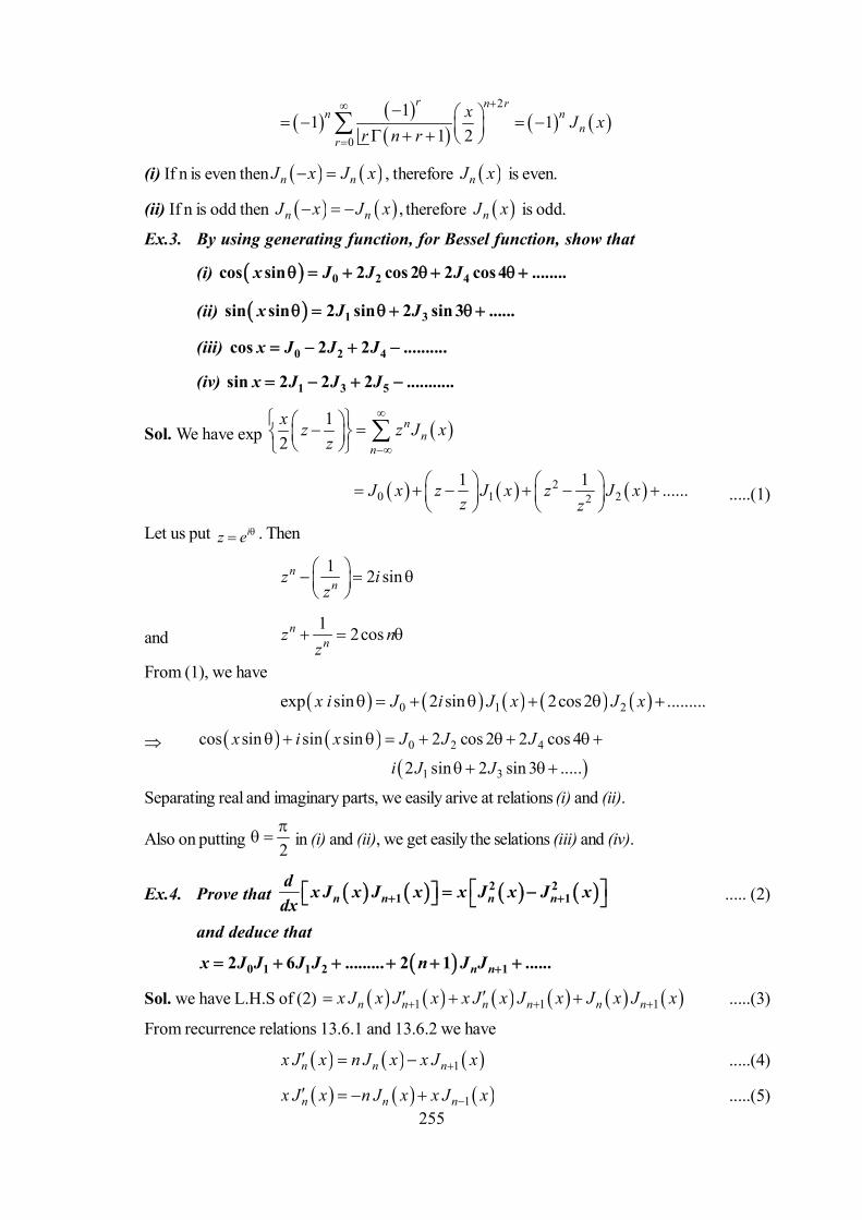
255
2
0
11 1
1 2
r n rn n
nr
x J xr n r
(i) If n is even then n nJ x J x , therefore nJ x is even.
(ii) If n is odd then ,n nJ x J x therefore nJ x is odd.
Ex.3. By using generating function, for Bessel function, show that
(i) 0 2 4cos sin 2 cos 2 2 cos 4 ........x J J J
(ii) 1 3sin sin 2 sin 2 sin 3 ......x J J
(iii) 0 2 4cos 2 2 ..........x J J J
(iv) 1 3 5sin 2 2 2 ...........x J J J
Sol. We have exp 12
nn
n
x z z J xz
20 1 22
1 1 ......J x z J x z J xz z
.....(1)
Let us put iz e . Then
1 2 sinnnz i
z
and1 2cosnnz n
z
From (1), we have
0 1 2exp sin 2 sin 2cos 2 .........x i J i J x J x
0 2 4
1 3
cos sin sin sin 2 cos 2 2 cos 4
2 sin 2 sin 3 .....
x i x J J J
i J J
Separating real and imaginary parts, we easily arive at relations (i) and (ii).
Also on putting 2
in (i) and (ii), we get easily the selations (iii) and (iv).
Ex.4. Prove that 2 21 1n n n n
d x J x J x x J x J xdx ..... (2)
and deduce that
0 1 1 2 12 6 ......... 2 1 ......n nx J J J J n J J
Sol. we have L.H.S of (2) 1 1 1n n n n n nx J x J x x J x J x J x J x .....(3)
From recurrence relations 13.6.1 and 13.6.2 we have
1n n nx J x n J x x J x .....(4)
1n n nx J x n J x x J x .....(5)
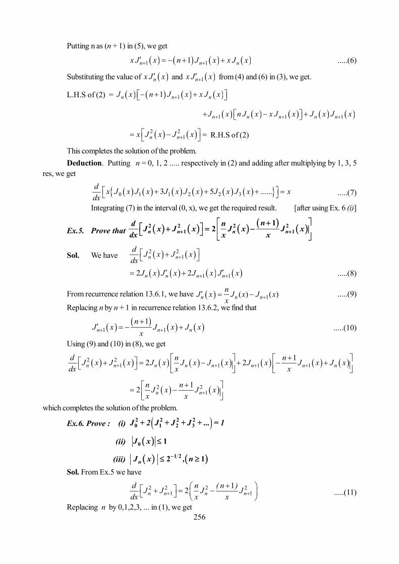
256
Putting n as (n + 1) in (5), we get
1 11n n nx J x n J x x J x .....(6)
Substituting the value of nx J x and 1nx J x from (4) and (6) in (3), we get.
L.H.S of (2) = 11n n nJ x n J x x J x
1 1 1n n n n nJ x n J x x J x J x J x
2 21n nx J x J x R.H.S of (2)
This completes the solution of the problem.Deduction. Putting n = 0, 1, 2 ..... respectively in (2) and adding after multiplying by 1, 3, 5
res, we get
0 1 1 2 2 33 5 ......d x J x J x J x J x J x J x xdx
.....(7)
Integrating (7) in the interval (0, x), we get the required result. [after using Ex. 6 (i)]
Ex.5. Prove that 2 2 2 21 1
12n n n n
nd nJ x J x J x J x
dx x x
Sol. We have 2 21n n
d J x J xdx
1 12 2n n n nJ x J x J x J x .....(8)
From recurrence relation 13.6.1, we have 1( ) ( )n n nnJ x J x J xx .....(9)
Replacing n by n + 1 in recurrence relation 13.6.2, we find that
1 11
n n nn
J x J x J xx
.....(10)
Using (9) and (10) in (8), we get
2 21 1 1 1
12 2n n n n n n n nd n nJ x J x J x J x J x J x J x J xdx x x
2 21
12 n nn nJ x J xx x
which completes the solution of the problem.
Ex.6. Prove : (i) 2 2 2 20 1 2 3J + 2 J + J + J + ... = 1
(ii) 0 1J x
(iii) 1 22 1nJ x , n
Sol. From Ex.5 we have
2 2 2 21 1
12n n n nd n ( n )J J J Jdx x x
.....(11)
Replacing n by 0,1,2,3, ... in (1), we get
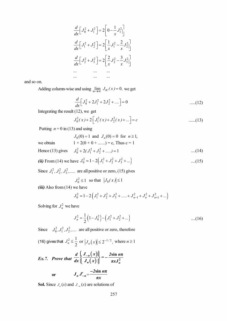
257
2 2 20 1 1
12 0d J J Jdx x
2 2 2 21 2 1 2
1 22d J J J Jdx x x
2 2 2 22 3 2 3
2 32d J J J Jdx x x
... ... ...... ... ...
and so on.Adding column-wise and using lim 0n nJ ( x ) , we get
2 2 20 1 22 2 0d J J J ....
dx .....(12)
Integrating the result (12), we get2 2 20 1 22J ( x ) J ( x ) J ( x ) ... c ......(13)
Putting n = 0 in (13) and using
0 (0) 1 and (0) 0 for 1,nJ J n we obtain 1 + 2(0 + 0 + ......) = c, Thus c = 1
Hence (13) gives 2 2 20 1 22 1J ( J J .....) ....(14)
(ii) From (14) we have 2 2 2 20 1 2 31 2 ...J J J J ....(15)
Since 2 2 21 2 3J , J , J ,..... are all positive or zero, (15) gives
20 1J so that 0 1J ( x )
(iii) Also from (14) we have
2 2 2 2 2 2 20 1 2 3 1 11 2 n n nJ J J J ..... J J J ...
Solving for 2nJ we have
2 2 2 20 1 2
1 12nJ J J J ... ....(16)
Since 2 2 20 1 2J ,J ,J ,.... are all positive or zero, therefore
(16) gives that 2 12nJ or 1 22 /
nJ x , where n 1
Ex.7. Prove that 2
sin πn
n n
J xd 2 n=dx J x πxJ
or n nJ J =sin π2 nπx
Sol. Since nJ (x) and nJ (x) are solutions of

258
2 2
2 21 1 0d y dy n y ,x dxdx x
therefore2
21 1 0n n n
nJ J J ,x x
...(17)
and2
21 1 0n n n
nJ J Jx x
...(18)
Multiplying (17) by nJ and (18) by Jn and substracting, we get
1 0n n n n n n n nJ J J J J J J Jx ...(19)
Let n n n nu J J J J .
Then (19) reduces to1 10 uu ux u x
Integrating we get log u = log ax or
aux
where a is arbitrary constant or
n n n naJ J J Jx
2 41
2 2 2 2 4 2 2 2 42 1
n nn
nx xx ....
n . n nn
1 31 2 41
2 2 2 2 4 2 2 2 42 1
n nn
nn x n x
nx ....n . n nn
2 41
2 2 2 2 4 2 2 2 42 1
n nn
nx xx ....
n . n nn
211 41 2
2 2 2 2 4 2 2 4 22 1
nnn
nn x( n )x anx ...
n . n n xn
.....(20)
Comparing the coefficients of 1x on both sides of (20), we get
1 2 2
1 1 1n sin na n n
n n n n n
(using 1sin z
z z
)
Thus 22sinn n n n
n n
J J J J nJ x J

259
22 sinn
n n
Jd ndx J x J
Self-Learning Exercise-I
1. J0 (x) is a Bessel’s function of order ....... .
2. ......n nn
d x J x xdx
.
3. Write generating function for Bessel function Jn (x) .4. J–n (x) = (– 1)n ........ .5. Write differential equation for the Bessel function Jn (x).
6. 1 1 ...........n nx J x J x .
7. Jn (x) is even function if n is .......
8. 0
lim ...........nnx
x J x
13.7 Addition Theorem
Statement : It n is a positive integer, then
0 1
1n
rn n n r r n r r n r
r rJ x y J x J y J x J y J y J x
...(1)
Proof : we have 1exp2
nn
n
xJ x z zz
1 1exp2 2
nn
n
x yJ x y z z exp zz z
r sr s
r sz J x z J y
Now equating the coefficient of zn on both sides, keeping in mind that the terms containing zn onR.H.S. are obtained by taking s = n – r and by making r vary from – to thus
n r n rr
J x y J x J y
...(2)
where n is any integer.
or 1
0 1r r
n
n r n r n r n rr r r n
J x y J x J y J x J y J x J y
...(3)
Now 1
r n rr
J x J y
1
p n pp
J x J y
(writing – r = p)
1
1 pp n p
pJ x J y
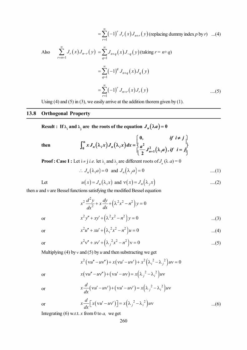
260
1
1 rr n r
rJ x J y
(replacing dummy index p by r) ...(4)
Also 1
r n rr n
J x J y
1n q q
qJ x J y
(taking r = n+q)
1
1 qn q q
qJ x J y
1
1 rn r r
rJ x J y
....(5)
Using (4) and (5) in (3), we easily arrive at the addition thorem given by (1).
13.8 Orthogonal Property
Result : If i and j are the roots of the equation 0nJ a
then n i n i
n i
, if i jx J x J x dx a J a , if i j
2
201
0
2Proof : Case I : Let i j i.e. let i and j are different roots of Jn (a) = 0
0n iJ a and 0n jJ a ....(1)
Let n iu x J x and n jx J x ....(2)then u and v are Bessel functions satisfying the modified Bessel equation
2
2 2 2 22 0d y dyx x x n y
dxdx
or 2 2 2 2 0x y xy x n y ...(3)
or 2 2 2 2 0ix u xu x n u ...(4)
or 2 2 2 2 0jx x x n ...(5)
Multiplying (4) by and (5) by u and then substracting we get
2 2 2 2 0i jx u u x u u x u
or 2 2j ix u u u u x u
or 2 2j i
dx u u u u x udx
or 2 2j i
dx x u u x udx
...(6)
Integrating (6) w.r.t. x from 0 to a, we get

261
2 200
a aj i xu dx x u u ...(7)
Using (2), (7) gives 2 20
aj i n i n jxJ x J x dx
0
a
n j n i n i n jx J x J x J x J x
n j n i n i n ja J a J a J a J a = 0 [using (1)]
Since i j the above equation gives
00
an i n jxJ x J x dx if i j ....(8)
Case II : Let i = j (equal roots). Multiplying (4) by 2u, we have
22 2 2 22 2 2 0ix u u x u x n uu
or 22 2 2 2 2 2 2 22 0i id x u n u x u xudx
or 22 2 2 2 2 2 2 22 i idxu x u n u x udx
....(9)
Integrating (9) w.r.t. x from 0 to a, we get
22 2 2 2 2 2 2 20 0
2aa
i ixu dx x u n u x u ....(10)
Using the relation Jn (0) = 0 and (1) and (2), we have
2 20
2a
i n ixJ x dx 2 2 22 2 2 2
0
a
n i n i i n ix
x J x n J x x J x
or 22 2 20 at
2a
i n i n ix a
xJ x dx a J x
....(11)
From recurrence relation 13.6.1, we have
1n n nd nJ x J x J xdx x ...(12)
Replace x by ix in (12), we have
or
1n i
n i n ii i
d J x n J x J xd x x
or
11 n i
n i n ii i
d J x n J x J xdx x
1n i n i i n inJ x J x J xx
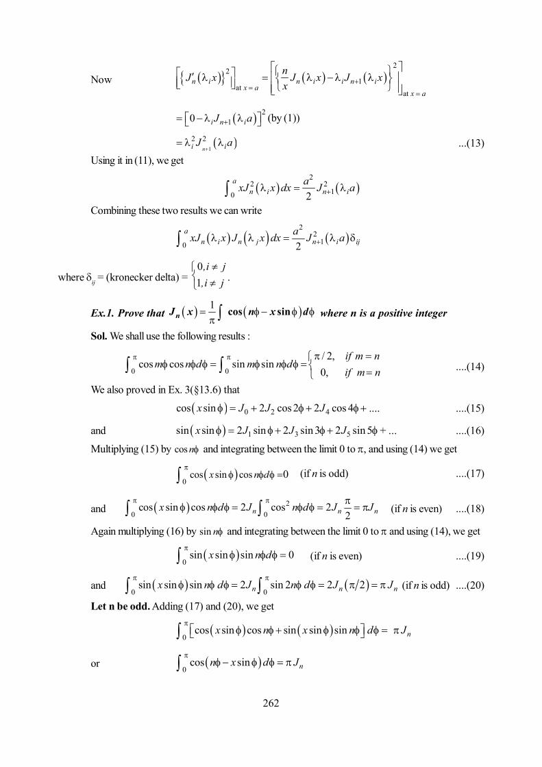
262
Now 2
21
atat
n i n i i n ix a
x a
nJ x J x J xx
210 i n iJ a (by (1))
1
2 2ni iJ a
...(13)Using it in (11), we get
2
2 210 2
an i n i
axJ x dx J a Combining these two results we can write
2
210 2
an i n j n i ij
axJ x J x dx J a
where ij = (kronecker delta) = 01
,i j,i j
.
Ex.1. Prove that 1 cos sinnJ x n x d where n is a positive integer
Sol. We shall use the following results :
0 0
/ 2,cos cos sin sin
0,if m n
m n d m n dif m n
....(14)
We also proved in Ex. 3(§13.6) that
0 2 4cos sin 2 cos 2 2 cos 4x J J J .... ....(15)
and 1 3 5sin sin 2 sin 2 sin 3 2 sin 5x J J J + ... ....(16)
Multiplying (15) by cos n and integrating between the limit 0 to , and using (14) we get
0
cos sin cos 0x n d
(if n is odd) ....(17)
and 20 0
cos sin cos 2 cos 22n n nx n d J n d J J
(if n is even) ....(18)
Again multiplying (16) by sin n and integrating between the limit 0 to and using (14), we get
0
sin sin sin 0x n d
(if n is even) ....(19)
and 0 0
sin sin sin 2 sin 2 2 2n n nx n d J n d J J
(if n is odd) ....(20)
Let n be odd. Adding (17) and (20), we get
0
cos sin cos sin sin sin nx n x n d J
or 0
cos sin nn x d J
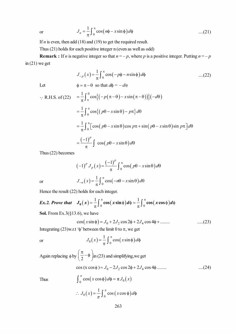
263
or 0
1 cos sinnJ n x d
....(21)
If n is even, then add (18) and (19) to get the required result.Thus (21) holds for each positive integer n (even as well as odd)Remark : If n is negative integer so that n = – p, where p is a positive integer. Putting n = – p
in (21) we get
0
1 cos sinpJ x p n d
....(22)
Let so that d= – d
R.H.S. of (22) 01 cos sinp x d
0
1 cos sinp x p d
0
1 cos sin cos sin sin sinp x p p x p d
1cos sin
p
p x d
Thus (22) becomes
0
11 cos sin
pp
pJ x p x d
or 0
1 cos sinnJ x n x d
Hence the result (22) holds for each integer.
Ex.2. Prove that 0 0
1 1J x x d x d0 cos sin cos cos
Sol. From Ex.3(§13.6), we have
0 2 4cos sin 2 cos 2 2 cos 4 ........x J J J .....(23)Integrating (23)w.r.t ‘’ between the limit 0 to , we get
or 0 0
1 cos sinJ x x d
Again replacing by 2
in (23) and simplifying,we get
cos (x cos ) 0 2 42 cos 2 2 cos 4J J J ........ ....(24)
Thus 00cos cos πx d J x
0 0
1 cos cosJ x x d

264
Ex.3. Prove that
02
2n
n nn n
dJ x x J xd x
Sol. Substituting the value of J0 (x) in series in R.H.S, we have
R.H.S
2
2 0
12
1 2
r rnn
nr
d xxr rd x
2
0
12
1 2
rn rn
n rr
d txr rdt
2
0
12
2
r r nn
rr
tx
r r n
2
0
11
1 2
r n rn
r
xr n r
1 nn nJ x J x
Ex.3. If, Prove that 0 2 20
1axe J bx dxa b
Sol. Using series representation for the Bessel function and changing the order of integration andsummation, we find that
22
0 20 00
1 2r rax r ax
r
bI e J bx dx x e dx
r
2
2 2 10
1 2 2 1r r
rr
b r
r a
(using the def. of gamma function)
Applying gamma duplication formula for 2 1r and simplifying, we find that
2
20
1 21r
r
r
bIa r a
1 22
2 2 2
1 11 ba a a b
13.9 Integral Representation of Bessel Functions
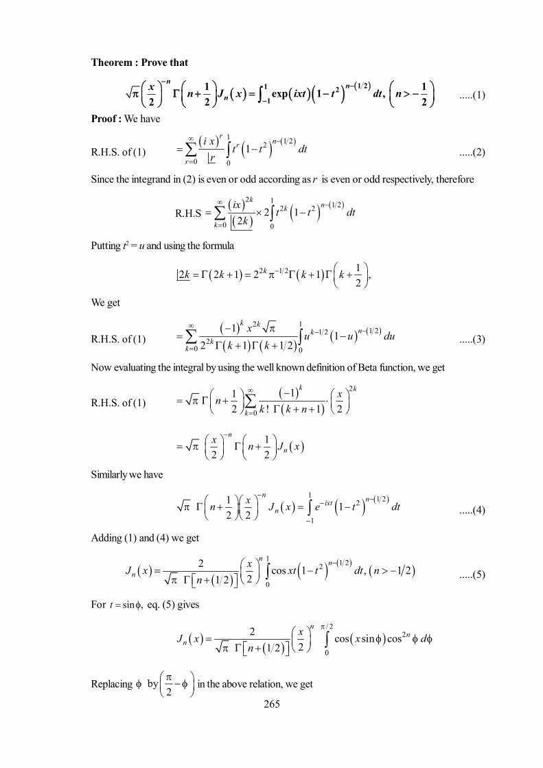
265
Theorem : Prove that
1 21 21
1 1exp 1 ,2 2 2
n nn
x n J x ixt t dt n
.....(1)
Proof : We have
R.H.S. of (1) 1 1 22
0 0
1r
nr
r
i xt t dt
r
.....(2)
Since the integrand in (2) is even or odd according as r is even or odd respectively, therefore
R.H.S 2 1 1 22 2
0 0
2 12
knk
k
ixt t dt
k
Putting t2 = u and using the formula
2 1 2 12 2 1 2 1 ,2
kk k k k
We get
R.H.S. of (1)
12
1 21 22
0 0
11
2 1 1 2
k knk
kk
xu u du
k k
.....(3)
Now evaluating the integral by using the well known definition of Beta function, we get
R.H.S. of (1)
2
0
112 ! 1 2
k k
k
xnk k n
12 2
n
nx n J x
Similarly we have
1 1 22
1
1 12 2
n nixtn
xn J x e t dt
.....(4)
Adding (1) and (4) we get
1 1 22
0
2 cos 1 , 1 221 2
n nn
xJ x xt t dt nn
.....(5)
For sin ,t eq. (5) gives
/ 2
2
0
2 cos sin cos21 2
nn
nxJ x x d
n
Replacing by2
in the above relation, we get

266
2
2
0
2 cos cos sin21 2
nn
nxJ x x d
n
13.10 An Important Integral
Theorem : Prove that
2
2 20 1 03 20
4 2a a ax a x J kx dx J ak J akk k
.....(1)
Proof : We know that 1n n
n nd x J x x J xdx
Replacing x by kx, we get
1n n
n nd x J kx kx J kxdx .....(2)
Integrating (2) w.r.t. x in the interval (0, a), we get
10
an n
n nx J kx dx a J ka .....(3)
Now, 2 2 2 30 0 0
0 0 0
a a a
x a x J ax dx a x J kx dx x J kx dx
3 2
1 10
aa x dJ ak x J kx dxk k dx
[Using (3) with n = 1 for first integral and (2) with n = 1 for second inte-
gral]
3
2 21 1 100
1 2a aa J ak x xJ kx x J kx dx
k k
3 3
21 1 22 0
2 aa a dJ ak J ak x J kx dxk k dxk
2
222a J axk
....(4)
Also we have the recurrence relation
1 12 n n nnJ x x J x J x ....(5)
Taking n = 1 and replacing x by kx in (5), we find that
2 1 02J kx J kx J kxkx
Substituting the value of J2(kx) in (4), we easily get the integral (1).
Self-Learning Exercise-II

267
1. 2 21 2 1 2J x J x = .............
2. The relation 10 1J x J x is true /false
3. 1 2 .......J x
4. 0
cos sin ..........n x d
5. 0 ...., 1J x n
6. ...., 1nJ x n
13.11 Summary
In this unit we studied the Bessel’s differential equation and its solution. Also we proved the im-portant properties such as recurrence relations, generating function, orthogonal property, integrals repre-sentation for the Bessel function.
13.12 Answers to Self- Learning Exercises
Exercise-1
1. 0 2. Jn-1(x)
3. 12
nn
n
xexp z J x zz
4. Jn (x)
5. 2
2 2 22 0d y dyx x x n y
dxdx 6. 2nJn(x)
7. even 8.1
2 !n nExercise-II
1.2x 2. true
3.2 sin xx
4. nJ x
5. 1 6. 1 22
13.13 Exercise
1. Prove that 1 22 cosJ x xx
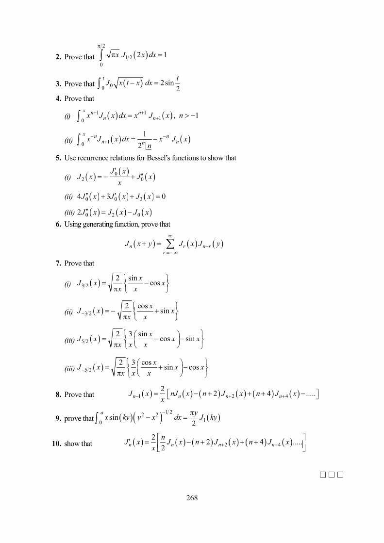
268
2. Prove that 2
1 20
2 1x J x dx
3. Prove that 002sin
2t tJ x t x dx
4. Prove that
(i) 1 110
, 1x n n
n nx J x dx x J x n
(ii) 10
12
x n nn nnx J x dx x J x
n
5. Use recurrence relations for Bessel’s functions to show that
(i) 02 0
J xJ x J x
x
(ii) 0 0 34 3 0J x J x J x
(iii) 0 2 02J x J x J x 6. Using generating function, prove that
n r n rr
J x y J x J y
7. Prove that
(i) 3 22 sin cosxJ x xx x
(ii) 3 22 cos sinxJ x xx x
(iii) 5 22 3 sin cos sinxJ x x xx x x
(iii) 5 22 3 cos sin cosxJ x x xx x x
8. Prove that 1 2 42 2 4 .....n n n nJ x nJ x n J x n J xx
9. prove that 1 22 2
10sin
2a yx ky y x dx J ky
10. show that 2 42 2 4 .....
2n n n nnJ x J x n J x n J x
x
269
Unit 14 : Hermite PolynomialsStructure of the Unit
14.0 Objective
14.1 Introduction
14.2 Hermite Differential Equation and Its Solution
14.3 Generating Function
14.4 Hypergeometric Form
14.5 Recurrence Formulas
14.6 Rodrigue’s Formula
14.7 Orthogonal Property
14.8 Summary
14.9 Answers to Self-Learning Exercises
14.10 Exercise
14.0 Objective
Here you will study Hermite polynomials its definition and important properties such as recur-
rence relations, generating function, orthogonal property, Rodrigue’s formula etc.
14.1 Introduction
Hermite polynomials occur in the study of wave mechanics and other physical problems. We
start with the Hermite differential equation and its solution. Then we develop and study properties of
Hermite polynomials. We also illustrate the properties with the help of solved problems.
14.2 Hermite Differenential Equation and Its Solution
Hermite’s equation is2
2 2 2 0d y dyx nydxdx
.....(1)
where n is any integer For solving equation (1), we use Frobenius method.
Let 00
, 0k rr
ry a x a
.....(2)
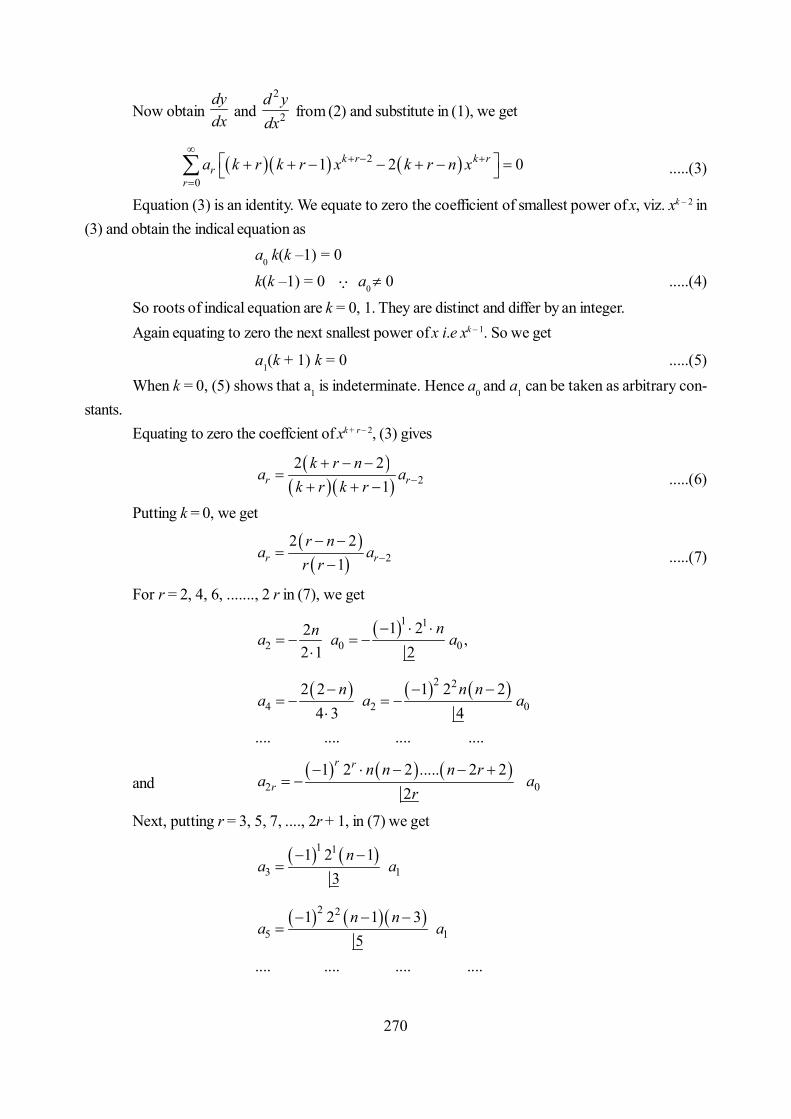
270
Now obtain dydx and
2
2d ydx
from (2) and substitute in (1), we get
2
01 2 0k r k r
rr
a k r k r x k r n x
.....(3)
Equation (3) is an identity. We equate to zero the coefficient of smallest power of x, viz. xk – 2 in(3) and obtain the indical equation as
a0 k(k –1) = 0
k(k –1) = 0 a0 0 .....(4)
So roots of indical equation are k = 0, 1. They are distinct and differ by an integer.Again equating to zero the next snallest power of x i.e xk – 1. So we get
a1(k + 1) k = 0 .....(5)When k = 0, (5) shows that a1 is indeterminate. Hence a0 and a1 can be taken as arbitrary con-
stants.Equating to zero the coeffcient of xk + r – 2, (3) gives
22 2
1r rk r n
a ak r k r
.....(6)
Putting k = 0, we get
2
2 21r r
r na a
r r
.....(7)
For r = 2, 4, 6, ......., 2 r in (7), we get
1 1
2 0 01 22 ,
2 1 2nna a a
2 2
4 2 02 2 1 2 2
4 3 4n n n
a a a
.... .... .... ....
and
2 01 2 2 ..... 2 2
2
r r
rn n n r
a ar
Next, putting r = 3, 5, 7, ...., 2r + 1, in (7) we get
1 1
3 11 2 1
3n
a a
2 2
5 11 2 1 3
5n n
a a
.... .... .... ....
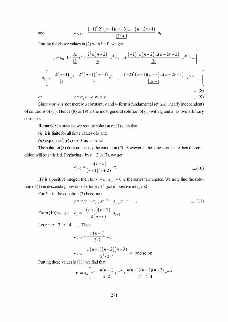
271
and
2 1 11 2 1 3 ...... 2 1
2 1
r r
rn n n r
a ar
Putting the above values in (2) with k = 0, we get
22 4 2
02 2 2 2 ... 2 221 ..... ....
2 4 2
rrn n n n n rny a x x x
r
23 5 2 1
12 1 2 1 3 2 1 3 ... 2 1
... ...3 5 2 1
rrn n n n n n r
a x x x xr
....(8)
or y = a0 v + a1w, say .....(9)Since v or w is not merely a constant, v and w form a fundamental set (i.e. linearly independent)
of solutions of (1). Hence (8) or (9) is the most general solution of (1) with a0 and a1 as two arbitraryconstants.
Remark : In practice we require solution of (1) such that(i) it is finite for all finite values of x and(ii) exp (1/2x2) y(x) 0 as x The solution (8) does not satisfy the condition (ii). However, if the series terminate then this con-
dition will be satistied. Replacing r by r + 2 in (7), we get
2
21 2r rr n
a ar r
.....(10)
If r is a positive integer, then for r = n, ar + 2 = 0 ie the series terminates. We now find the solu-tion of (1) in descending powers of x for n + (set of positive integers)
For k = 0, the equation (2) becomesy = anx
n + an –2 xn – 2 + an –4
xn – 4 + .... .....(11)
From (10) we get 21 2
2r rr r
a an r
Let r = n – 2, n – 4, ...... Then
2
12 2n n
n na a
.
4 2
1 2 32 2 4n n
n n n na a
and so on
Putting these values in (11) we find that
y 2 42
( 1) ( 1)( 2)( 3) ...2 2 2 2 4
n n nn
n n n n n na x x x
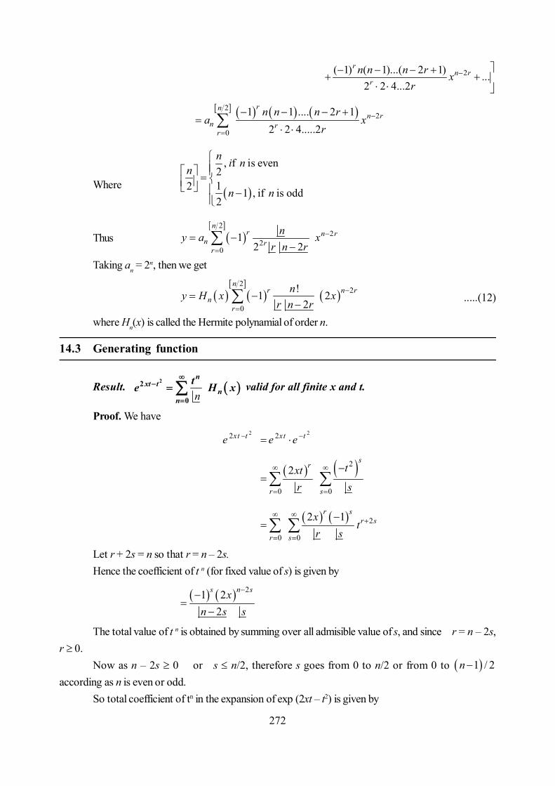
272
2( 1) ( 1)...( 2 1) ...2 2 4...2
rn r
rn n n r x
r
22
0
1 1 .... 2 12 2 4.....2
rnn r
n rr
n n n ra x
r
Where
, f is even212 1 , if is odd2
n i nn
n n
Thus 2
22
01
2 2
nr n r
n rr
ny a xr n r
Taking an = 2n, then we get
2
2
0
!1 22
nr n r
nr
ny H x xr n r
.....(12)
where Hn(x) is called the Hermite polynamial of order n.
14.3 Generating function
Result. n
xt tn
n
te H x22
0
n
valid for all finite x and t.
Proof. We have22xt te 22xt te e
2
0 0
2sr
r s
txtr s
2
0 0
2 1r sr s
r s
xt
r s
Let r + 2s = n so that r = n – 2s.Hence the coefficient of t n (for fixed value of s) is given by
21 22
s n sxn s s
The total value of t n is obtained by summing over all admisible value of s, and since r = n – 2s,r 0.
Now as n – 2s 0 or s n/2, therefore s goes from 0 to n/2 or from 0 to 1 / 2naccording as n is even or odd.
So total coefficient of tn in the expansion of exp (2xt – t2) is given by
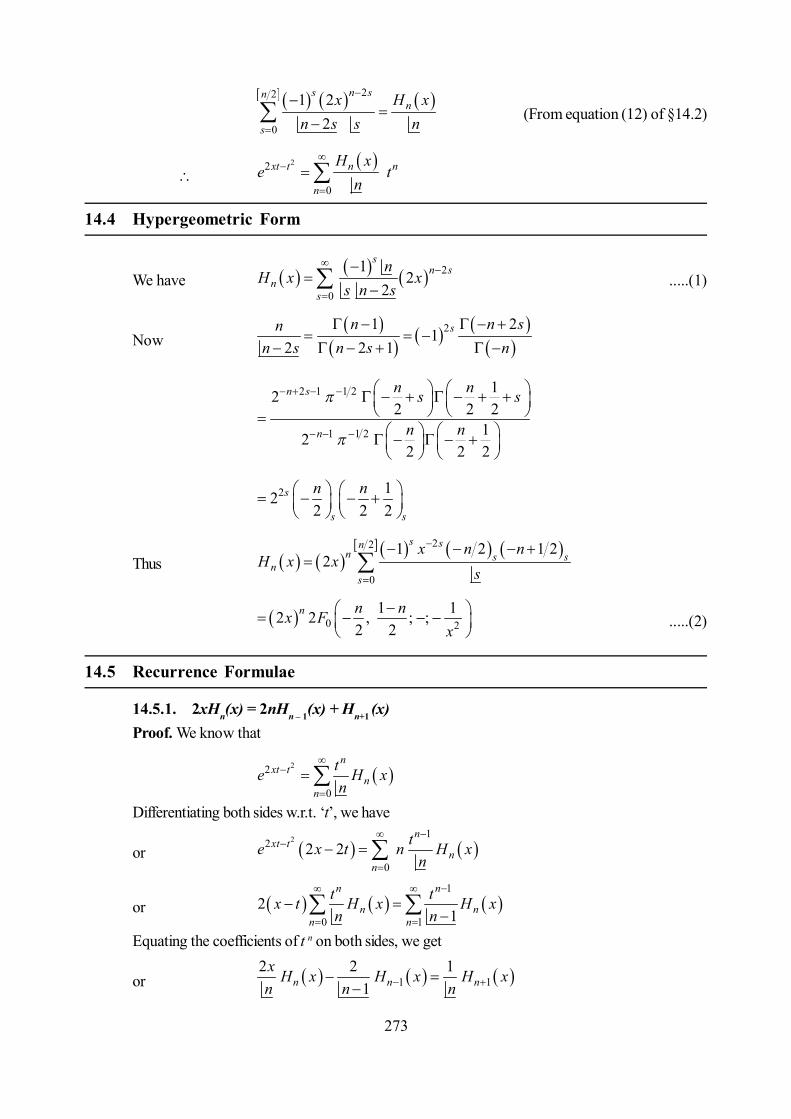
273
22
0
1 22
s n snn
s
x H xn s s n
(From equation (12) of §14.2)
22
0
nxt t n
n
H xe t
n
14.4 Hypergeometric Form
We have 2
0
12
2
sn s
ns
nH x x
s n s
.....(1)
Now
21 21
2 2 1sn n sn
n s n s n
2 1 1 2
1 1 2
122 2 2
122 2 2
n s
n
n ns s
n n
2 122 2 2
s
s s
n n
Thus 22
0
1 2 1 22
s snn s s
ns
x n nH x x
s
0 21 12 2 , ; ;
2 2n n nx F
x
.....(2)
14.5 Recurrence Formulae
14.5.1. 2xHn(x) = 2nHn – 1(x) + Hn+1 (x)Proof. We know that
22
0
nxt t
nn
te H xn
Differentiating both sides w.r.t. ‘t’, we have
or 2 1
2
02 2
nxt t
nn
te x t n H xn
or 1
0 12
1
n n
n nn n
t tx t H x H xn n
Equating the coefficients of t n on both sides, we get
or 1 12 2 1
1n n nx H x H x H xn n n
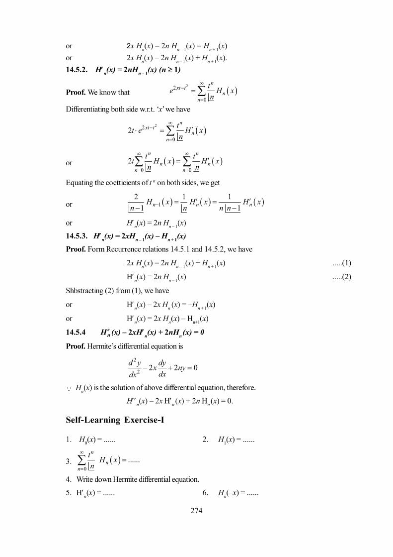
274
or 2x Hn(x) – 2n Hn – 1(x) = Hn + 1(x)or 2x Hn(x) = 2n Hn – 1(x) + Hn + 1(x).14.5.2. Hn(x) = 2nHn – 1(x) (n 1)
Proof. We know that 22
0
nxt t
nn
te H xn
Differentiating both side w.r.t. ‘x’ we have
22
02
nxt t
nn
tt e H xn
or 0 0
2n n
n nn n
t tt H x H xn n
Equating the coetticients of t n on both sides, we get
or 12 1 1
1 1n n nH x H x H xn n n n
or Hn(x) = 2n Hn – 1(x)
14.5.3. Hn(x) = 2xHn – 1(x) – Hn + 1(x)
Proof. Form Recurrence relations 14.5.1 and 14.5.2, we have
2x Hn(x) = 2n Hn – 1(x) + Hn + 1(x) .....(1)
Hn(x) = 2n Hn – 1(x) .....(2)
Shbstracting (2) from (1), we have
or Hn(x) – 2x Hn (x) = –Hn + 1(x)
or Hn(x) = 2x Hn(x) – Hn+1(x)
14.5.4 nH (x) – 2xHn(x) + 2nHn (x) = 0
Proof. Hermite’s differential equation is2
2 2 2 0d y dyx nydxdx
Hn(x) is the solution of above differential equation, therefore.
Hn(x) – 2x Hn (x) + 2n Hn (x) = 0.
Self-Learning Exercise-I
1. H0(x) = ...... 2. H1(x) = ......
3. 0
......n
nn
t H xn
4. Write down Hermite differential equation.
5. Hn(x) = ...... 6. Hn(–x) = ......

275
Ex.1. Prove that nH (x) = 4n(n – 1) Hn – 2(x)
Sol. From rcurrence relation 14.5.2, we have
Hn(x) = 2n Hn – 1(x)
Differentiating with respect to x, we get''nH (x) = 2n 1
'nH (x)
Again using recurrence relation 14.5.2, we find that
nH (x) = 2n × 2(n – 1) Hn – 2 (x)
= 4n (n – 1) Hn – 2 (x)
Ex.2. Prove that if m < n
m m
nn mm
d H x n H xn mdx2
Sol. We know that
22
0
nx t t
nn
te H xn
or 22
0
m n m mxt t
nm m mn
d t d de H xndx dx dx
or 22
02
mn mm nx t t
m mn
d H xt dt en dx dx
or 0 0
2mr n m
m nr m m
r n
d H xt t dt H xr n dx dx
or 0 0
2mr m n
nmr m
r n
d H xt tH xr n dx
If r + m = n
[Note that r 0 n – m 0 or m n]
or 0
2mn n
nmn m m
n m n
d H xt tH xn m n dx
Equating the coefficient of t n on both sides, we get
2 1 mmn
n m m
d H xH x
n m n dx
or 2 mmn
n m m
d H xn H xn m dx
Ex.3. Prove that
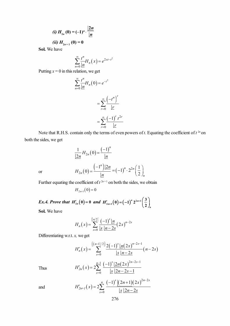
276
(i) H2n (0) = (–1)n n
n2
(ii) H2n + 1 (0) = 0Sol. We have
22
0
nxt t
nn
t H x en
Putting x = 0 in this relation, we get
2
00
nt
nn
t H en
0
rn
r
t
r
2
0
1 r r
r
tr
Note that R.H.S. contain only the terms of even powers of t. Equating the coefficient of t 2n onboth the sides, we get
2
11 02
n
nHn n
or
2
1 20
n
n
nH
n
2 11 2
2n n
n
Further equating the coefficient of t 2n +1 on both the sides, we obtain 2 1 0 0nH
Ex.4. Prove that 2 0 0nH and 2 12 1
30 1 22
n nn
n
H
Sol. We have
2
2
0
12
2
snn s
ns
nH x x
s n s
Differentiating w.r.t. x, we get
2 11 2
0
2 1 22
2
s n sn
ns
n xH x n s
s n s
Thus 2 2 11
0
1 2 22
2 2 1
s n sn
2ns
n xH x
s n s
and 2 2
0
1 2 1 22
2 2
s n sn
2n+1s
n xH x
s n s

277
Hence 0 02nH
and 1 2 1
0n
2n+1
nH
n
2 1 31 22
n n
n
(by using gamma duplication formula)
14.6 Rodrigues Formula for Hn(x)
To Prove that n x
n xn n
d eH x e
dx
2
21
Proof. We have
0 1, ..... .....0 1
n nH x H x t H xf x t t
n
where 22 22, x txt t xf x t e e e
0
,nn
nnt
f x t H xn H x
nt
2 2
0
x tn x
n n
t
e eH x
t
22
0
x tnx
nt
e et
.....(1)
Let x – t = u that is t = x – u x = u at t = 0
Also x – t = u t u
22
1n ux tn
nn n
eet u
22
0
1n xx tn
nn n
t
eet x

278
2
1n x
nn
d e
dx
From (1), we get 2
21
n xn x
n n
d eH x e
dx
14.7 Orthogonal Property of Hermite Polynomials
Theorem. Prove that x nn m mne H x H x dx n
2
2 where mn is Kronicar delta
or 2 0
2x
n m n
if m ne H x H x dx
n if m n
Proof. We know that
22
0
nxt t
nn
te H xn
22
0
mxs s
mm
se H xs
2 22 2
0 0
n mxt t xs s
n mn m
t se e H x H xn s
1 1n mH x H x
n m = Coefficent of tnsm in the expansion of
2 22 2xt t xs se e
So 2x
n me H x H x dx n m
times the coefficent of tnsm in the expansion of
2 2 22 2x xt t xs se e e dx
.....(1)
Now2 2 22 2x xt t xs se e e dx
2 2 2 2 2t s x xt rse e
2 222 2 2x x t s t s t st se e dx
22 22 2 2x x t s t s t st se e e dx

279
22 x t sste e dx
22st ue e du
[where x – (t + s) = u and hence dx = du]
2
0
2 nst
n
ste
n
0
2nn n
ns t
n
Here the series on right-hend side contains the terms having the equal powers of t and s. There-fore the coefficent of tn sm, (m n) will be zero. Equating the coefficent of tn sm on both sides of aboveresult,we get
2
0xn me H x H x dx
where m n
and from (1), we have
2x
n me H x H x dx n m
2n
n
2nn , where m = n
Hence 2
2x nn m mne H x H x dx n
Ex.1. Prove that 2
212 exp .4
n nn
dH x xdx
Sol. We have
222
txt x
d ete
dx
2
212
t xt x
d ete
dx
Differentiating w.r.t. x
2 2 21 22
t x txd d e t edx dx

280
2 2 21 12 2
t x t xd d e t edx dx
2
2 2 212
t x t xd e t edx
Hence by symmetry for n terms, we get
2 212
nt x n t xd e t e
dx
.....(2)
Now,
22
21exp.4
t xd edx
22
0
1 14
nt x
n
d en dx
22
0
1 12
n nt x
n
d en dx
2 2
0
1 nn t x
nt e
n
[from (2)]
2 2
0
1 nt x n
ne t
n
2 2
0
1 nt x
ne t
n
2 22 2t x t x t te e e
or 2
20
1 1exp. 24
n
n
d t xndx
0
n
nn
t H xn
Equating the coefficent of tn on both sides we get
21 1 1exp. 2
4n n
nd x H xdx n n
212 exp.
4n n
ndH x xdx
which completes the solution of the problem.
Ex.2. Expand xn in a series of Hermite polynomials
Sol. We have
22
0
nxt t
nn
te H xn
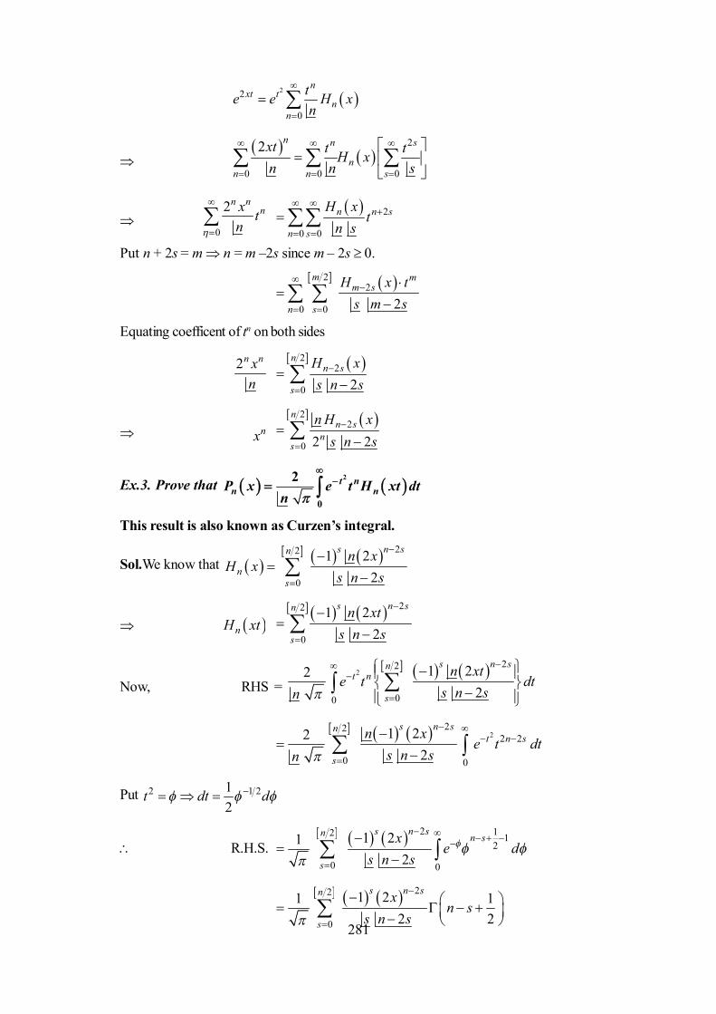
281
22
0
nxt t
nn
te e H xn
2
0 0 0
2 n n s
nn n s
xt t tH xn n s
0
2n nnx t
n
2
0 0
n n s
n s
H xt
n s
Put n + 2s = m n = m –2s since m – 2s 0.
22
0 0 2
m mm s
n s
H x ts m s
Equating coefficent of tn on both sides
2n nxn
22
0 2
nn s
s
H xs n s
nx 2
2
0 2 2
nn s
ns
n H xs n s
Ex.3. Prove that t nn nP x e t H xt dt
n
2
0
2
This result is also known as Curzen’s integral.
Sol.We know that 22
0
1 22
s n sn
ns
n xH x
s n s
nH xt 22
0
1 22
s n sn
s
n xts n s
Now, RHS =
222
00
1 222
s n snt n
s
n xte t dt
s n sn
2
222 2
0 0
1 222
s n snt n s
s
n xe t dt
s n sn
Put 2 1 212
t dt d
R.H.S. 2 12 12
0 0
1 212
s n sn n s
s
xe d
s n s
22
0
1 21 12 2
s n sn
s
xn s
s n s

282
22
0
11 2 2
2 1 2
s n sn
s
n sxs n s
1 2
222
0
1 2 1 22
s n snn s
s
xs n s
= Pn(x) (by definition of Legendre polynomials)
Ex.4. Show that 2
0exp 2
nn s
sn
H x txt t H x t
n
Sol. Consider
0 0
n sn s
n s
H x tn s
0 0
n s snn
n s
H x tn s s
0 0
1 s n s snns
n s
n H x t un s t
0 0
sn nn s
n s
nH x tn s t
0
1nn
n
n
H x tn t
0
nn
n
H x tn
22x t te
22 22 x txt te e
22
0
ssxt t
s
H x te
s
Comparing the coeffiecient of !
s
s
, we get the required result.
Ex.5. Establish
ncnn
n
c H x t c c txt Fn xt
2
2 0 20
1 41 2 , ; ;2 2 2 1 2
.....(3)
Sol. We have
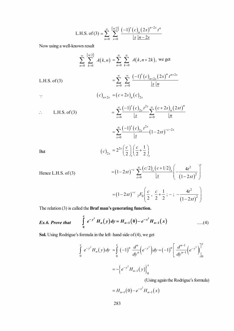
283
L.H.S. of (3) 22
0 0
1 22
s n s nnn
n s
c x ts n s
Now using a well-known result
2
0 0,
n
n kA k n
0 0, 2 ,
n kA k n k
we get
L.H.S. of (3) 2
2
0 0
1 2s n n sn s
n s
c x ts n
2n sc 22 n sc s c
L.H.S. of (3) 2
2
0 0
1 2 2s nss n
s n
c t c s xts n
222
0
11 2
s sc ss
s
c txt
s
But 2sc2 12
2 2 2s
s s
c c
Hence L.H.S. of (3)
2
20
2 1 2 41 21 2
sc s s
s
c c txts xt
2
2 0 21 41 2 , ; ;
2 2 2 1 2c c c txt F
xt
The relation (3) is called the Braf man’s generating function.
Ex.6. Prove that 2 2
1 10
0x
y xn n ne H y dy H e H x
.....(4)
Sol. Using Rodrigue’s formula in the left–hand side of (4), we get
2
0
xy
ne H y dy 2 21
10 0
1 1xx n n
n ny yn n
d de dy edy dy
2
10
xy
ne H y
(Using again the Rodrigue’s formula)
2
1 10 xn nH e H x
284
Self-Learning Exercise-II
1. 2
............xn me H x H x dx if m n
2. Write down Rodriques formulas for Hn(x).3. H2n + 1(0) = ...........
14.8 Summary
In this unit, we studied the Hermite differential equation and Hermile polynomials. We also stud-ied recurrence relation, generating function, Rodrigue, formula and orthogonal property for Hermite poly-nomials.
14.9 Answers to Self-Learning Exercises
Exercise I
1. 22xt te
2.2
2 2 2 0d y dyx ydxdx
3. 12 nnH x
Exercise II1. 0
2. 2
21
n xn x
n x n
d eH e
dx
3. 0
14.10 Exercise
1. Evaluate 2x
m nxe H x H x dx
(m n) [Ans : 0]
2. Prove that 5 35 32 160 120H x x x x
3. Prove that 22 4 2H x x
4. Express 4 3 22 2 3H x x x x x in terms of Hermite polynomials.
5. Prove that 1n n nx H n n H x n H x
285
6. Prove that 2 22 122
x nnx e H x dx n n
7. Show that
1 11
0 2 ! 2
nk k n n n n
k nk
H x H y H x H y H x H yk y x n
8. Evaluate 2 21 12n x t n
nxe e t P x t dt
[Ans : Hn(x)]
9. Evaluate 2
,xm nxe H x H x dt m n
[Ans : 0]
10. If 2 2n ,xx e Hn x then prove that
(i) ,ψ ψ 2 if 1nm n m nx x dx n m n
(ii) 1
0, if 1
ψ ψ 2 , if 1
2 1 , if 1
nm n
n
m n
x x dx n m n
n m n
11. Using the expansion of x n in a series of Hermite polynomials, show that
2 2
2e 2x n kn k
nx H x dxk
286
Unit 15 : Laguerre Polynomials15.0 Objective
15.1 Introduction
15.2 Definition
15.3 Generating Function for Ln (x)
15.4 Recurrence Formulae for Ln (x)
51.5 Rodrigue’s Formula for Ln (x)
15.6 Orthogonal Property for Ln (x)
15.7 Associated Laguerre Polynomial : Definition
15.8 Generating Function for Associated Laguerre Polynomial
15.9 Recurrence Formulae for Associated Laguerre Polynomial
15.10 Rodrigue’s Formula for Associated Laguerre Polynomial
15.11 Orthogonal Property for Associated Laguerre Polynomial
15.12 Summary
15.13 Answer to Self-Learning Exercises
15.14 Exercise
15.0 Objective
In this unit you will study Laguerre and associated Laguerre polynomials and their important prop-erties such as generating function, orthogonal property, Rodrigue’s formula, recurrence relations etc.
15.1 Introduction
The purpose of this unit is to introduce and study the Laguerre and associated Laguerre polyno-mials. We shall state and prove certain important properties associated with these classes of polynomi-als.
15.2 Laguerre’s Differential Equation and Its Solution
THe Laguerre differential equation of order n is
2
2 1 0,d y dyx x nydxdx
.....(1)
where n is a positive integer

287
Now we apply the method of Frobenius for its solution which is finite for all values of x andwhich tends to no faster than ex/2 as x .
Proceeding on lines similar to explained in the case of Legendre, and Hermite polynomials, wefind that if we assume the solution of (1) in the form
0
rr
ry a x
.....(2)
then
0 20
1n
r r
r
ny a xn r r
.....(3)
will be solution of equation (1). Taking a0 = 1, the corresponding solution of equation (1) is known asLaguerre polynomial of order n, and which is denoted by Ln (x). Thus
20
1n
r rn
r
nL x xn r r
1 1 ; 1;F n x .....(4)
Some times we take a0 as n , then alternative definition of Laguerre polynomials is
2
20
1n
r rn
r
nL x x
n r r
.....(5)
15.3 Generating Function for Ln (x)
Theorem : Show that
1
01
x tt
nn
n
e L x tt
Proof : Using the exponential series we have
1
1
x ttet
0
1 11 1
r
r
x tt r t
1
0
11
rrr r
rx t t
r
0 0
11 r sr rs
r s
r tx tr s
2
0 0
1 r r r s
r s
r s x t
r s
....(1)
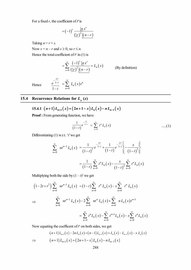
288
For a fixed r, the coefficient of tn is
21
rr n x
r n r
Taking n = r + s.Now s = n – r and s 0, so r n.Hence the total coefficient of tn in (1) is
20
1 r r
ns
n xL x
r n r
(By definition)
Hence1
1
x ttet
0
nn
nL x t
15.4 Recurrence Relations for Ln (x)
15.4.1 1 11 2 1n n nn L x n x L x n L x
Proof : From generating function, we have
11
1
xtte
t
0
nn
nt L x
.....(1)
Differentiating (1) w.r.t. ‘t’ we get
1
0
nn
nnt L x
1 12 2
1 111 1
xt x tt t xe e
tt t
20 0
11 1
n nn n
n n
xt L x t L xt t
Multiplying both the side by (1 – t)2 we get
2 1
01 2 n
nn
t t nt L x
0 01 n n
n nn n
t t L x x t L x
1 1
0 0 02n n n
n n nn n n
nt L x nt L x n L x t
1
0 0 0
n n nn n n
n n nt L x t L x x t L x
Now equating the coefficent of tn on both sides, we get
1 1 11 2 1n n n n n nn L x n L x n L x L x L x x L x
1 11 2 1n n nn L x n x L x n L x

289
15.4.2 1n n nx L x n L x n L x
Proof : From generating function
0
nn
nt L x
111
xtte
t
.....(2)
Differentiating w.r.t. ‘x’ we get
0
nn
nt L x
11
1 1
xtt te
t t
or 0
nn
nt L x
01
nn
n
t t L xt
or 0
1 nn
nt t L x
0
nn
nt t L x
or 1
0 0
n nn n
n nt L x t L x
1
0
nn
nt L x
Equating the coefficients of tn on both sides, we get
1 1n n nL x L x L x
or 1 1 1n n nL x L x L x .....(3)
Differentiating Recurrence relation 15.4.1, we find that
1 11 2 1n n n nn L x n x L x L x n L x .....(4)Replacing n by (n + 1) in (3), we obtain
1n n nL x L x L x .....(5)
Putting the value of 1nL x and 1nL x from (3) and (5) in (4) we get
1 n nn L x L x 12 1 n n n nn x L x L x n L x L x
n n n nn L x n L x L x L x
112 n n n n n nnL x L x x L x L x n L x n L x
On simplification, we get 1n n nx L x n L x n L x
15.4.3 1
0
n
n rr
L x L x
Proof : From generating function
0
nn
nt L x
111
xtte
t
.....(6)
Differentiating (6) w.r.t. ‘x’, we get
or 0
nn
nt L x
11
1 1
xtt te
t t
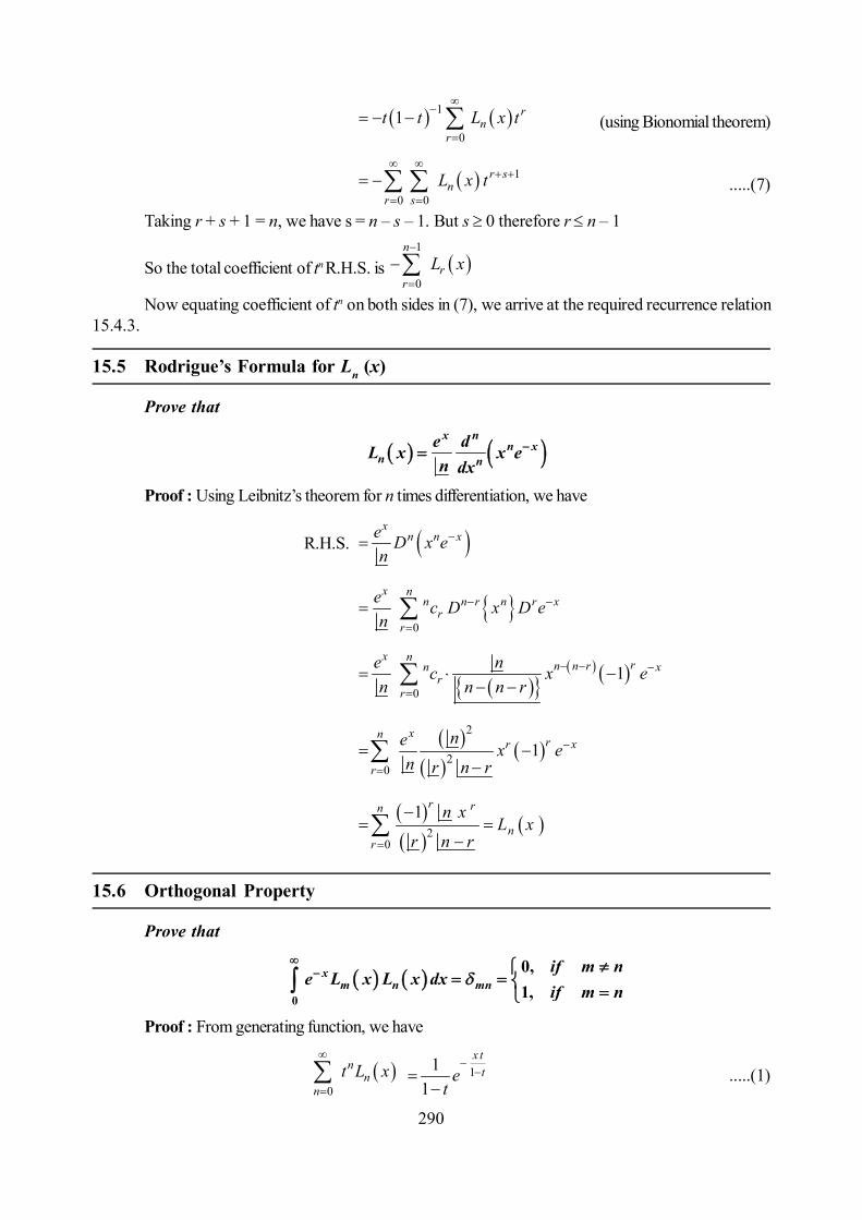
290
1
01 r
nr
t t L x t
(using Bionomial theorem)
1
0 0
r sn
r sL x t
.....(7)
Taking r + s + 1 = n, we have s = n – s – 1. But s 0 therefore r n – 1
So the total coefficient of tn R.H.S. is 1
0
n
rr
L x
Now equating coefficient of tn on both sides in (7), we arrive at the required recurrence relation15.4.3.
15.5 Rodrigue’s Formula for Ln (x)
Prove that
x n
n xn n
e dL x x en dx
Proof : Using Leibnitz’s theorem for n times differentiation, we have
R.H.S. x
n n xe D x en
0
x nn n r n r x
rr
e c D x D en
01
x nrn n rn x
rr
e nc x en n n r
2
20
1xn
rr x
r
ne x en r n r
20
1 r rn
nr
n xL x
r n r
15.6 Orthogonal Property
Prove that
0
0,1,
xm n mn
if m ne L x L x dx
if m n
Proof : From generating function, we have
0
nn
nt L x
11
1
x tte
t
.....(1)

291
0
mm
ms L x
11
1
x sse
s
.....(2)
Multiplying (1) and (2), we get
0 0
n mn m
n mL x t L x s
1 11 11 1
t sxt se
t s
0 0 0
x n mm n
n me L x L x dx t s
1 1
0
11 1
t sxx t se e dx
t s
1
1 1
0
11 1
t sxt se dx
t s
11 1
0
11 1 1
1 1
t sxt se
t st st s
1
1 1
0
1 111 1 1 1
t sxt st s
et s t s t ts s st
1 0 11 s t ts t ts s st
11 11
stst
21 ..... .....nst st st
Equating the coefficients of tn sn on both sides, we get
0
xm ne L x L dx
0 if m n .....(3)
and equating the coefficient of tn sm, we get
20
xne L x dx
= 1
That is 0
1xn me L x L x dx
(when m = n) .....(4)
Combining (3) and (4), we get 0
xm n mne L x L x dx

292
Ex.1. Prove that
1 11
nst
n0
e L t dt =s s
Sol. L.H.S. 200
1 r rnst
r
n te dt
r n r
1 12
0 0
1 rnst r
r
ne t dt
n r r
2 1
0
1 1rn
rr
n rsn r r
0
11 1rn
rr
ns n r r s
0
1 1 1 11r nn
nr
rc
s s s s
= R.H.S.
Ex.2. Prove that (i) Ln (0) = 1, (ii) 0nL n and (iii) 10
2nn n
L
Sol. We know that
111
x tte
t
0
nn
nt L x
....(5)
Taking x = 0 in (5), we get
or 11 t 0
0nn
nt L
or0
n
nt
00n
nn
t L
Equating coefficients of tn on both sides, we get
1 0nL
(ii) From Laguerre differential equation, we havexy + (1 – x) y + ny = 0
If Ln(x) is the solution of this equation then
1n n nx L x x L x n L x = 0Putting x = 0, we get
0nL 0nn L
1n [from (i)]
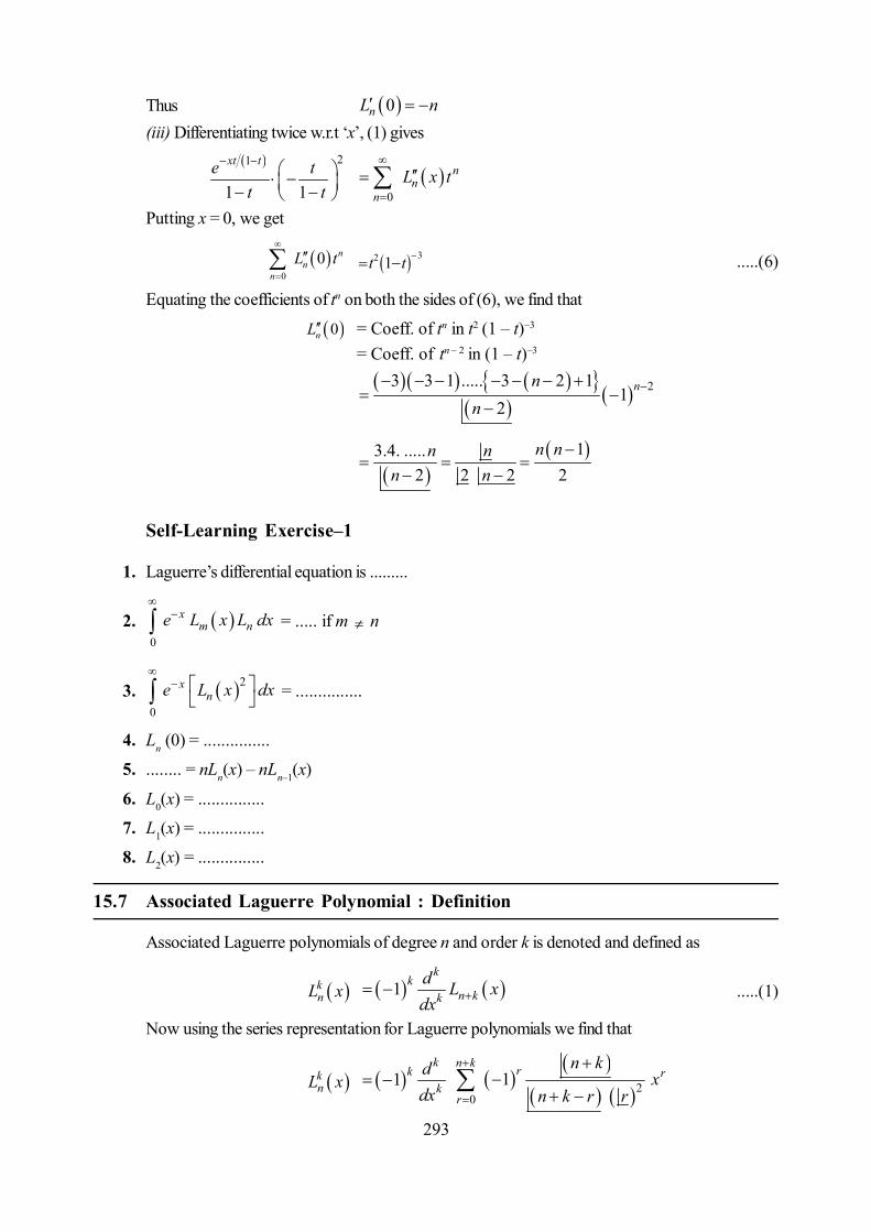
293
Thus 0nL n
(iii) Differentiating twice w.r.t ‘x’, (1) gives 21
1 1
xt te tt t
0
nn
nL x t
Putting x = 0, we get
0
0 nn
nL t
32 1t t .....(6)
Equating the coefficients of tn on both the sides of (6), we find that
0nL = Coeff. of tn in t2 (1 – t)–3
= Coeff. of tn – 2 in (1 – t)–3
23 3 1 ..... 3 2 1
12
nnn
13.4. .....
2 2 2 2n nn n
n n
Self-Learning Exercise–1
1. Laguerre’s differential equation is .........
2. 0
xm ne L x L dx
= ..... if m n
3. 20
xne L x dx
= ...............
4. Ln (0) = ...............
5. ........ = nLn(x) – nLn–1(x)
6. L0(x) = ...............
7. L1(x) = ...............
8. L2(x) = ...............
15.7 Associated Laguerre Polynomial : Definition
Associated Laguerre polynomials of degree n and order k is denoted and defined as
knL x 1
kk
n kkd L xdx .....(1)
Now using the series representation for Laguerre polynomials we find that
knL x 1
kk
kddx
20
1n k r r
r
n kx
n k r r
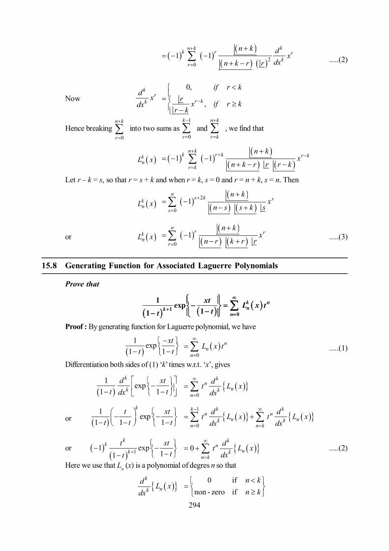
294
20
1 1kn kk r rk
r
n k d xdxn k r r
.....(2)
Nowk
rk
d xdx
0,
,r k
if r kr x if r k
r k
Hence breaking 0
n k
r
into two sums as
1
0
k
r
and
n k
r k
, we find that
knL x
1 1n k
k r k r k
r k
n kx
n k r r r k
Let r – k = s, so that r = s + k and when r = k, s = 0 and r = n + k, s = n. Then
knL x
2
01
ns k s
s
n kx
n s s k s
or knL x
0
1n
r r
r
n kx
n r k r r
.....(3)
15.8 Generating Function for Associated Laguerre Polynomials
Prove that
10
1 exp11
k nnk
n
xt L x ttt
Proof : By generating function for Laguerre polynomial, we have
1 exp
1 1xt
t t
0
nn
nL x t
.....(1)
Differentiation both sides of (1) ‘k’ times w.r.t. ‘x’, gives
1 exp
1 1
k
kd xt
t tdx
0
kn
nkn
dt L xdx
or 1 exp
1 1 1
kt xtt t t
1
0
k kkn n
n nk kn n k
d dt L x t L xdx dx
or 11 exp
11
kk
kt xt
tt
0k
nnk
n k
dt L xdx
.....(2)
Here we use that Ln (x) is a polynomial of degres n so that
k
nkd L xdx
0 ifnon - zero if
n kn k

295
Multiplying by (2) by (–1)k then we get
1 exp11
k
kt xt
tt
1k
k nnk
n k
dt L xdx
1 exp11
k
kt xt
tt
0
1k
k s ks kk
s
dt L xdx
(Taking s as new variable such that n = s + k i.e. s = n – k so when n = k, s = 0 and when n
tends to, s also tends to )
1 exp11
k
kt xt
tt
0
1k
kk ss kk
s
dt L x tdx
or 11 exp
11 kxt
tt
0
1k
k nn kk
n
d L x tdx
( The limit remain same so we can change the variable from s to n)
1
0
1 exp11
k nnk
n
xt L x ttt
15.9 Recurrence Relations for knL x
15.9.1 11
k k kn n nL x L x L x
Proof : We know that knL x
0
1n r
r
n k
n r k r r
.....(1)
Replacing n by (n – 1) in (1), we find that
1knL x
1
0
1 11
1
rnr r
r
n kx
n r r k r
.....(2)
Replacing k by (k – 1) in (1), we get
1knL x
0
1 1
1
rnr
r
n kx
n r k r r
.....(3)
Using (2) and (3), we have
11
k kn nL x L x
1
0
1 1
1
rnr
r
n kx
n r k r r
0
1 1
1
rn
r
r
n kx
n r k r r
1
0
1 1
1
rnr
r
n kx
n r k r r
1
0
1 1
1
rnr
r
n kx
n r k r r
1 1
1
n nn k x
n n k n n

296
1
0
1 1
1 1
rnr
r
n k n kxn r k r r k r n r
1 n nx
n
1
0
1 1r nr nn
r
n k x xn r k r r n
0
1 r rn
r
n k xn r k r r
knL x [by (1)]
15.9.2 1 11 2 1k k kn+ n n-n + L x = n + k + - x L x - n + k L x
Proof : From recurrence relation 15.4.1 for Laguerre polynomial we have
1 11 2 1n n nn L x n x L x nL x ...(4)
Replacing n by (n + k) in (4), we get
1 11 2 2 1n k n x n kn k L x n k x L x n k L x
Differentiating k times, the above equation becomes
11 2 2 1k k
n k n kk kd dn k L x n k L xdx dx
1
k k
n k n kk kd dxL x n k L xdx dx ...(5)
Using Leibnitz’s theorem, we get
k
n kkd xL xdx
1
1 1
k kk
n k n kk kd dL x x c L xdx dx
1
1
k k
n k n kk kd dx L x k L xdx dx
...(6)
Using (6) in (5) and then multiplying both sides by (–1)k, we get
11 1k
kn kk
dn k L xdx
1 2 2 1k
kn kk
dn k L xdx 1
kk
n kkdx L xdx
1
11 111
kk
n kkdk L xdx
11k
kn kk
dn k L xdx ....(7)
But from definition 1k
kkn n kk
dL x L xdx ....(8)
Using (8) in (7), we get

297
11 2 2 1k kn nn k L x n k L x
11 1
k k kn n nxL x kL x n k L x
.....(9)
Replaceing n by n + 1 in 15.9.1, we get
11 1
k k kn n nL x L x L x
or 11 1
k k kn n nL x L x L x .....(10)
Eliminating 11
knL from (10) and (9), we get
1 1 11 2 2 1k k k k k kn n n n n nn k L x n k L x x L x k L x L x n k L x
That is 1 11 2 1k k kn n nn L x n k x L x n k L x
15.9.3 k kn n
d L x L xdx
11
Proof : We know that knL x
0
1 r rn
r
n k xn r k r r
.....(11)
Differentiating both side of (11) w.r.t. ‘x’ we get
L.H.S.= kn
d L xdx
1
0
1 r rn
r
n k rx
n r k r r
1
1
11
r rn
r
n k xn r k r r
11
0
11 1
s sn
s
n k xn s k s s
(Taking r – 1 = s)
1
0
1 1 11
1 1
s sn
s
n k x
n s k s s
kn
d L xdx 1
1 R.H.SknL x
15.10 Rodrigue’s Formula for knL x
Theorem : Prove that
x k n
k n k xn n
e x dL x x xn dx
Sol :
R.H.S. x k
n x n ke x D e xn
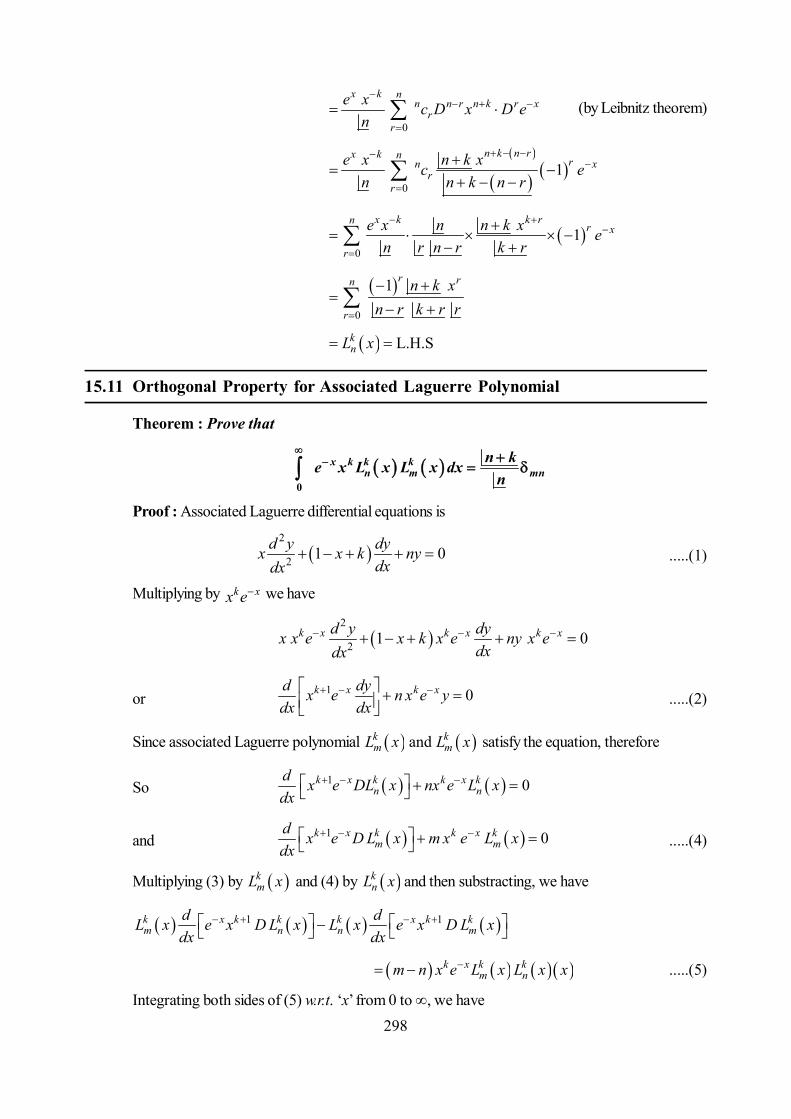
298
0
x k nn n r n k r x
rr
e x c D x D en
(by Leibnitz theorem)
0
1n k n rx k n rn x
rr
e x n k xc en n k n r
0
1x k k rn
r x
r
e x n n k x en r n r k r
0
1 r rn
r
n k xn r k r r
L.H.SknL x
15.11 Orthogonal Property for Associated Laguerre Polynomial
Theorem : Prove that
x k k kn m mn
n ke x L x L x dxn
0
Proof : Associated Laguerre differential equations is
2
2 1 0d y dyx x k nydxdx
.....(1)
Multiplying by k xx e we have
2
2 1 0k x k x k xd y dyx x e x k x e ny x edxdx
or 1 0k x k xd dyx e n x e ydx dx
.....(2)
Since associated Laguerre polynomial andk km mL x L x satisfy the equation, therefore
So 1 0k x k k x kn n
d x e DL x nx e L xdx
and 1 0k x k k x km m
d x e D L x m x e L xdx
.....(4)
Multiplying (3) by kmL x and (4) by k
nL x and then substracting, we have
1 1k x k k k x k km n n m
d dL x e x D L x L x e x D L xdx dx
k x k km nm n x e L x L x x .....(5)
Integrating both sides of (5) w.r.t. ‘x’ from 0 to , we have
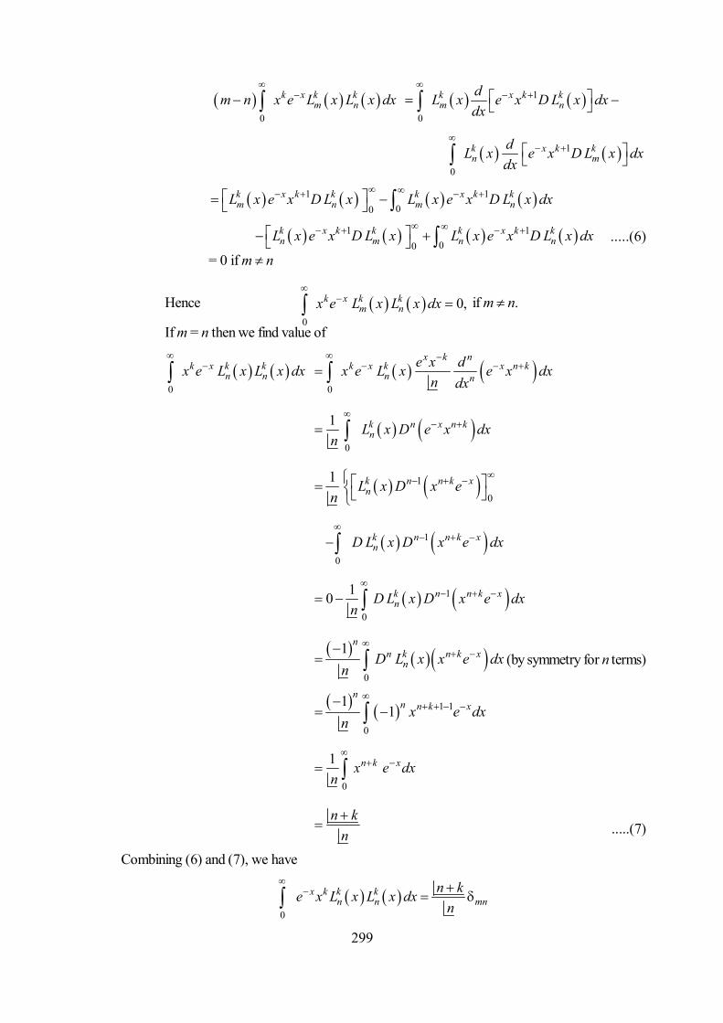
299
0
k x k km nm n x e L x L x dx
1
0
k x k km n
dL x e x D L x dxdx
1
0
k x k kn m
dL x e x D L x dxdx
1 100
k x k k k x k km n m nL x e x D L x L x e x D L x dx
1 1
00k x k k k x k kn m n nL x e x D L x L x e x D L x dx
.....(6)= 0 if m n
Hence 0
0,k x k km nx e L x L x dx
if m n.
If m = n then we find value of
0
k x k kn nx e L x L x dx
0
x k nk x k x n k
n ne x dx e L x e x dx
n dx
0
1 k n x n knL x D e x dx
n
1
0
1 k n n k xnL x D x e
n
1
0
k n n k xnD L x D x e dx
1
0
10 k n n k xnD L x D x e dx
n
0
1 nn k n k x
nD L x x e dxn
(by symmetry for n terms)
1 1
0
11
nn n k xx e dx
n
0
1 n k xx e dxn
n kn
.....(7)
Combining (6) and (7), we have
0
x k k kn n mn
n ke x L x L x dxn

300
Ex.1. Prove that 1t k x k k
n n nx
e L t dt e L x L x
Sol. Integrating by parts taking e–t as second function, we get
t kn
x
e L t dt
t k t kn nx
x
e L t e DL t dt
x k t kn n
x
e L x e DL t dt
1
0
nx k t k
n rrx
e L x e L t dt
1
0
nk kn r
rDL t L t
1
0
nt k t k
n rrx x
e L t dt e L t dt
x kne L x .....(8)
or 0
nt k
nr x
e L t dt
x k
ne L x .....(9)
Subtracting (9) from (8), we get
or 1
0 00
n nt k t k t k
r n rr rx x x
e L t dt e L t dt e L t dt
or t kn
x
e L t dt
1
0 0
n nt k t k
r rr rx x
e L t dt e L t dt
or t kn
x
e L t dt
1x k x k
n ne L x e L [using (9)]
or t kn
x
e L t dt
1x k k
n ne L x L x
Ex.4. Establish the generating functions :
(i) 2
0
11 21
t nn n
n n
x t e J x t L x t
(ii)
1 10
1 ; 1 ;1 11
nnnc
n n
cx tF c L x ttt
Sol. (i) We have
0
11
nn
n n
L x t
0 0
11
k k nn
kn k
x tk n k

301
Using 0 0
,n k
A k n
0 0,
n kA k n k
, we get
0
11
nn
n n
L x t
0 0
11
k n k n
kn k
t xk n
0 0 1
kn
n k k
x ttn k
0 1 ;1 ;te F x t .....(10)We know that
2
0 1
2; 1 ;
1 4
n
n
z zJ z F nn
.....(11)
Using (11) in (9) we get the required generating function (i)(ii) We have
0 1
nnn
n n
cL x t
0 0
11
k k nnn
kn k
c x tk n k
0 0
11
k k n kn k
n k k
c x tk n
0 01
k nk n
kk n
c k tc x tk n
01
1
kc kk
k k
c x tt
k
1 11 ; 1 ;
11 cx tF c
tt
Ex.5. Prove that 1
0
n
n r n rr
L x y L x L y
Sol. We have
1 11 exp 1 exp1 1x t y tt t
t t
1 11 exp
1x y t
tt
Therefore
1
0
nn
nL x y t
0 0
n nn r
n rL x t L y t
0 0
nn
n r rn r
L x L y t
Comparing the coefficients of tn, we get the required result.
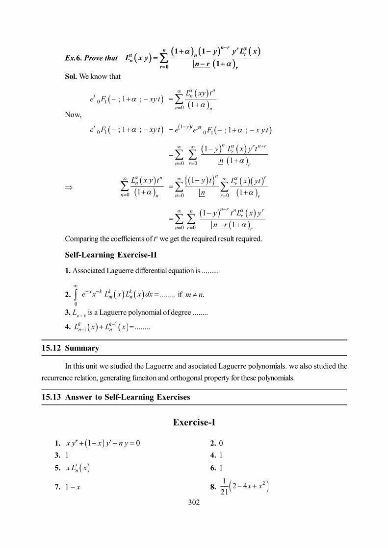
302
Ex.6. Prove that
n r rnrn
nr r
y y L xL x y
n r
0
1 11
Sol. We know that
0 1 ; 1 ;te F xy t
0 1
nn
n n
L xy t
Now,
0 1 ; 1 ;te F xy t 10 1 ; 1 ;y t yte e F x y t
0 0
11
n r n rr
n r r
y L x y tn
0 1
nn
n n
L x y t
0 0
11
n rr
n r r
y t L x ytn
0 0
11
n r n rnr
n r r
y t L x yn r
Comparing the coefficients of tn we get the required result required.
Self-Learning Exercise-II
1. Associated Laguerre differential equation is .........
2. 0
........x k k km ne x L x L x dx
if m n.
3. Ln + k is a Laguerre polynomial of degree ........
4. 11 ........k k
n nL x L x
15.12 Summary
In this unit we studied the Laguerre and asociated Laguerre polynomials. we also studied therecurrence relation, generating funciton and orthogonal property for these polynomials.
15.13 Answer to Self-Learning Exercises
Exercise-I
1. 1 0x y x y n y 2. 03. 1 4. 15. nx L x 6. 1
7. 1 – x 8. 21 2 421
x x

303
Exercise-II
1. 1 0x y x k y n y 2. 0
3. n + k 4. knL x
15.14 Exercise
1. Find the value of
(i) 3 50
xe L x L x dx
[Ans. 0]
(ii) 24
0
xe L x dx
[Ans. 1]
2. Express 10 – 23x + 10x2 – x3 in terms of Laguerre polynomials.[Ans. L0(x) + L1 (x) + 2L2 (x) + 6L3 (x) ]
3. Prove that 1y x
n n nx
e L y dy e L x L x
4. Show that
2 12
0
1 22 3 2
ntn
n nn
H tL n t x dx
5. Show that
0
1 11,2,3,......
1
n r n rnkn
r
k n xL x n
r n r k n r
6. Prove that
(i) 1 22 22 1 2n n
n nH x n L x
(ii) 2 1 1 2 22 1 1 2n n
n nH x n L x
7. Show that 1
221 222
0
11 22 4
tn n
n nn
tx t x H x t x dx L
8. Show that
0 !
nn ss
ns
L xL x
s
9. Show that
21
0
2 1x k kn
n ke x L x dx n k
n
10. Prove that 1 1
0 1
xm m m
n nm nx t L t dt x L x
m n

304
Reference Books
1. Differential Equations Vol. II
J.L. Bansal and H.S. Dhami,
Jaipur Publishing House, Jaipur.
2. Advanced Differential Equations
M.D. Raisinghania, S. Chand & Comp.,
New Delhi.
3. Calculus of Variations
Robert Weinstock,
Dover Publications.
4. Special Functions
R.K. Saxena and D.C. Gokhroo,
Jaipur Publishing House, Jaipur.
5. Special Functions
E.D. Rainville, Chelsea Publishing Comp.,Bronx , New York.


