
Understanding Visual Art with CNNs
Michael BaumerStanford University
Department of [email protected]
Derek ChenIndependent Researcher
https://[email protected]
Abstract
Previous work in computational visual art classificationhas relied on fixed, pre-computed features extracted fromraw images. In this work, we use convolutional neural net-works (CNNs) to classify images from a collection of 40,000digitized works of art according to artist, genre, and loca-tion. After some simple pre-processing and downsampling,we employ a modified VGGNet architecture to achieve bet-ter than state-of-the-art results on artist and genre classifi-cation (we could not find a literature benchmark for loca-tion identification). We obtain a test set accuracy of 62.2%on artist classification, 68.5% on genre classification, out-performing the best algorithms in the literature by 3% and10%, respectively.
Our results represent a step forward in the computa-tional understanding of visual art. We present a confusionmatrix for our artist classifier that reveals interesting quan-titative similarities between different artists. In addition, weproduce class optimization images for art of various genreswhich elucidate the quantitative features that distinguishvarious genres of art. We end by discussing possible ex-tensions that have potential to improve these results evenfurther.
1. IntroductionMany art museums have amassed and digitized very
large collections of human artwork. This presents animmense curatorial challenge to both understand famouspieces and attribute pieces of unknown origin based on char-acteristic features of individual artists and time periods. Analgorithm to identify the likely artist behind a work wouldbe useful to both museum curators and auction houses asone way of validating an acquisition of unknown prove-nance.
In addition, while expert art historians can recognize aparticular artist’s style or estimate the date of an unknownpiece, it is difficult for amateurs like ourselves to under-stand the image features that distinguish works of art. The
Figure 1. Example artwork found in our input catalog. Artist,genre and location truth labels for this image are ‘Michelangelo’,‘Religious’, and ‘Italian’, respectively.
main motivation for this project is to apply quantitativetechniques to increase our understanding of visual art.
To do this, we take images found in a catalog of ∼40, 000 works from the Web Gallery of Art (WGA) and useCNNs based on a modified VGG-Net architecture to predictthe artist, genre, and location (see Table 1 for examples ofeach) of a given work of art. An example input image, alongwith relevant truth data, from the WGA catalog is shown inFigure 1.
Our first goal is to achieve as high of accuracies as possi-ble in classifying works of art by artist, genre, and location,and compare to results from literature. Our second goal isto use methods learned in this course to better understandthe features of input images that lead to the classificationswe make.
To tackle these goals, we review previous work in sec-tion 2, 3 outline a modified VGGNet architecture in section4, describe our cross-validation strategy in section 5, de-scribe our classification results from our artist-, genre-, andlocation-classifying networks in section 6, discuss the im-plications of this work on artistic understanding in section7, and propose future extensions and improvements to thiswork in section 8.
1
Artist Technique Medium Genre LocationMichelangelo Painting Oil on canvas Religious Italian
Giotto Sculpture Fresco Portrait FrenchRembrandt Graphics Marble Landscape Dutch
Albrecht Durer Illumination Photograph Mythological Flemishvan Gogh Architecture Oil on wood Still life German
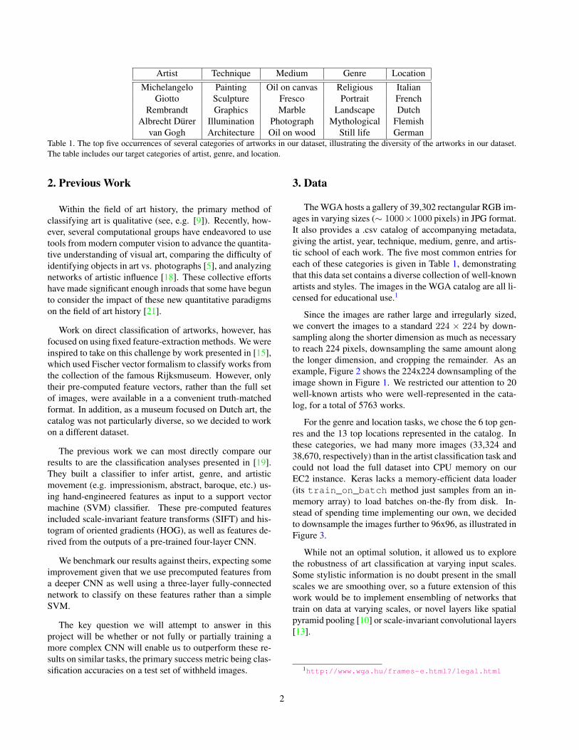
Table 1. The top five occurrences of several categories of artworks in our dataset, illustrating the diversity of the artworks in our dataset.The table includes our target categories of artist, genre, and location.
2. Previous Work
Within the field of art history, the primary method ofclassifying art is qualitative (see, e.g. [9]). Recently, how-ever, several computational groups have endeavored to usetools from modern computer vision to advance the quantita-tive understanding of visual art, comparing the difficulty ofidentifying objects in art vs. photographs [5], and analyzingnetworks of artistic influence [18]. These collective effortshave made significant enough inroads that some have begunto consider the impact of these new quantitative paradigmson the field of art history [21].
Work on direct classification of artworks, however, hasfocused on using fixed feature-extraction methods. We wereinspired to take on this challenge by work presented in [15],which used Fischer vector formalism to classify works fromthe collection of the famous Rijksmuseum. However, onlytheir pre-computed feature vectors, rather than the full setof images, were available in a a convenient truth-matchedformat. In addition, as a museum focused on Dutch art, thecatalog was not particularly diverse, so we decided to workon a different dataset.
The previous work we can most directly compare ourresults to are the classification analyses presented in [19].They built a classifier to infer artist, genre, and artisticmovement (e.g. impressionism, abstract, baroque, etc.) us-ing hand-engineered features as input to a support vectormachine (SVM) classifier. These pre-computed featuresincluded scale-invariant feature transforms (SIFT) and his-togram of oriented gradients (HOG), as well as features de-rived from the outputs of a pre-trained four-layer CNN.
We benchmark our results against theirs, expecting someimprovement given that we use precomputed features froma deeper CNN as well using a three-layer fully-connectednetwork to classify on these features rather than a simpleSVM.
The key question we will attempt to answer in thisproject will be whether or not fully or partially training amore complex CNN will enable us to outperform these re-sults on similar tasks, the primary success metric being clas-sification accuracies on a test set of withheld images.
3. Data
The WGA hosts a gallery of 39,302 rectangular RGB im-ages in varying sizes (∼ 1000×1000 pixels) in JPG format.It also provides a .csv catalog of accompanying metadata,giving the artist, year, technique, medium, genre, and artis-tic school of each work. The five most common entries foreach of these categories is given in Table 1, demonstratingthat this data set contains a diverse collection of well-knownartists and styles. The images in the WGA catalog are all li-censed for educational use.1
Since the images are rather large and irregularly sized,we convert the images to a standard 224 × 224 by down-sampling along the shorter dimension as much as necessaryto reach 224 pixels, downsampling the same amount alongthe longer dimension, and cropping the remainder. As anexample, Figure 2 shows the 224x224 downsampling of theimage shown in Figure 1. We restricted our attention to 20well-known artists who were well-represented in the cata-log, for a total of 5763 works.
For the genre and location tasks, we chose the 6 top gen-res and the 13 top locations represented in the catalog. Inthese categories, we had many more images (33,324 and38,670, respectively) than in the artist classification task andcould not load the full dataset into CPU memory on ourEC2 instance. Keras lacks a memory-efficient data loader(its train_on_batch method just samples from an in-memory array) to load batches on-the-fly from disk. In-stead of spending time implementing our own, we decidedto downsample the images further to 96x96, as illustrated inFigure 3.
While not an optimal solution, it allowed us to explorethe robustness of art classification at varying input scales.Some stylistic information is no doubt present in the smallscales we are smoothing over, so a future extension of thiswork would be to implement ensembling of networks thattrain on data at varying scales, or novel layers like spatialpyramid pooling [10] or scale-invariant convolutional layers[13].
1http://www.wga.hu/frames-e.html?/legal.html
2

Figure 2. The 224x224 downsampling of Michelangelo’s Creationof Adam used in the artists classifier.
Figure 3. The 96x96 downsampling of the same work, used ingenre and location classfication.
4. Methods
We implement our classifier using Keras, a recently-developed framework for building and training deep learn-ing models [7]. We chose Keras because of its simple APIto a Theano backend [2] [4], as well as the availability ofpre-trained weights for a VGGNet architecture [1]. Anotheradvantage of using Keras was that the code runs on bothCPUs and GPUs without any manual adaptation, which al-lowed us to iterate quickly on our local machines beforerunning larger jobs on Amazon EC2 g2.2xlarge instances.These instances use NVIDIA GRID K520 GPUs, with dataaccess provided by an external Elastic Block Store (EBS)volume.
As a baseline model, we use a modified VGGNet ar-chitecture (based on configuration “D” as recommended inclass) [20] initialized with fixed pre-trained weights from[1] in all the convolutional layers. We modify the vanillaVGG architecture by adding dropout and batch normaliza-tion layers between the fully-connected (FC) layers. A dia-
Figure 4. A schematic diagram of our modified VGGNet architec-ture. ReLU layers are omitted for brevity.
gram of our network architecture is shown in Figure 4.The convolutional blocks of our model (shown in red in
Figure 4) are formed from sequential blocks zero-paddinglayers, convolution layers, and activation layers. The bene-fit of using convolution blocks over fully-connected hiddenlayers is these blocks take into account the spatial layout ofthe input data, as well as reducing the number of parametersin the model.
Since VGGNet uses 3x3 filters with stride 1, we add onerow and column of zero-padding to the image before eachconvolutional layer to maintain the size of each image as itis passed through the network.
Finally, after each convolution layer, we use rectified lin-ear units (ReLU) activation layers, which have been shownto be superior to sigmoidal activations when training deepnetworks [16]. ReLU units introduce non-linearity into thenetwork by clipping negative activations to zero and neversaturating positive activations:
ReLU(x) = max(0, x) (1)
In addition to providing non-linearity, ReLU units, in con-trast to sigmoidal and tanh units which squash large valuesto ≈ 1, where the resulting gradients are nearly zero, helpavoid this vanishing gradient problem during backpropaga-
3

tion by continually increasing the gradient in conjunctionwith its final output.
The pooling blocks in our architecture (orange in Figure4) implement 2x2 max-pooling to progressively reduce thespatial size of the images by retaining only the maximumvalue in a 2x2 activation block that slides across the inputvolume with stride 2. Pooling reduces the number of pa-rameters needed for all downstream layers, which has thebenefit of lowering memory costs in addition to reducingthe potential for overfitting.
The second component of our network is blocks of denselayers that consist of fully-connected (FC) units, a batchnormalization layer, a ReLU activation, and a dropout layer.The FC layers compute a linear combination of input fea-tures xout = WTxin, as in a traditional neural network.The weight matrixW contains the learned parameters of thelayer, initialized according to the prescription given in [11].What makes the FC layers so effective in this context is thatthe inputs from the upstream convolutional filters containspatial structure from the input image that FC layers alonewould not be able to extract.
The batch normalization layer [12] serves to renormalizethe activations of a given layer to a unit Gaussian distribu-tion. This helps the later non-linearity perform better by en-suring that any weights that might have grown too large ortoo small are brought back to a reasonable size. The batchnormalization formula for a single batch is given by:
x =xin − E [xin]√V ar (xin)
(2)
xout = γx+ β (3)
where γ and β are learnable parameters of each batch thatallow the network to undo the normalization forced by thefirst equation if training shows it preferable. This can be ac-complished by setting γ =
√V ar (xin) and β = E [xin].
It is important to note that since both of these formulas aredifferentiable, we can backpropagate through them like anyother layer.
Lastly, these dense blocks also include two forms of reg-ularization. The fully-connected layers contain L2 regular-ization which penalizes weight vectors by adding a term tothe loss function (see Equation 5) of the form
λ∑
FC layers k
√∑i,j
(W(k)ij )2 (4)
where λ is a hyperparameter that sets the regularizationstrength.
The second form of regularization is dropout, whichmakes the network more robust by randomly (with someprobability pdrop) setting the activations of each node of the
upstream layer to zero. pdrop is a hyperparameter that weinclude in our cross-validation. By removing nodes fromthe model at each step, each remaining weight must now bemore robust in its contribution to the final prediction. There-fore, as with L2 regularization, we prefer weights with moreevenly distributed values.
The final component of our network is the loss function.We have chosen a softmax classifier which uses the cross-entropy loss function:
L =1
N
N∑i=1
(efyi∑efj
)(5)
This loss function will allow learning to continue even fromexamples it has already classified correctly. This is in con-trast to the SVM loss function, which returns zero loss oncethe target class score is greater than all others by a fixedmargin.
To optimize this loss function, we initially started withvanilla SGD with Nesterov momentum [17]. At the time,we were performing classification on three artists, andachieved a top validation accuracy of 77.6%. We decided toswitch over to using the Adam optimizer [14], which keepsa decaying average of past gradients, as well as squares ofgradients. These values are used to calculate the first-orderand second-order moments of the past gradients. UsingAdam on the initial 3-class task, we ended up with a topvalidation accuracy of 81.3% after 10 epochs, so we contin-ued using Adam for all future optimizations to save cross-validation time.
5. Training and Cross-ValidationOur cross-validation experiments consisted of sam-
pling three hyperparameters—learning rate, regularizationstrength, and dropout probability—over a broad range ofscales. Learning rate and L2 regularization strength weresampled uniformly in log-space, while dropout probabilitywas sampled directly from a uniform distribution to ensureunbiased exploration of parameter space.
We started by using random search rather than gridsearch to sample the parameter space more efficiently [3].During this time, a coarse search was made by training atleast 20 models per classification task with parameters cho-sen from a wide range of values, as described in Table 2.Because the goal was to simply determine what options dis-played favorable properties, such as a continuously decreas-ing validation loss, these networks were only run for justfour epochs.
Once we identified subsets of these ranges where we ob-tained reasonable results, we sampled more densely withina smaller range of possible values, as shown in Table 2.At this stage, we were more interested in seeing consistent
4

Hyperparameter Coarse Range Fine Range Artists Opt. Genres Opt. Locations Opt.
Learning Rate 10(−7,−2) 10(−6,−4) 1× 10⁻⁴ 1.2× 10⁻⁵ 8× 10⁻⁵
L2 Regularization Strength 10(−7,−2) 10(−5,−4) 8× 10⁻⁴ 1× 10⁻³ 5× 10⁻⁵
Dropout Probability (0.1,0.9) (0.3,0.5) 0.40 0.35 0.45Table 2. Ranges of tested hyperparameters for both coarse-grain and fine-grain cross-validation, along with the optimal values found foreach classification task.
progress in the right direction, so we ran each model up toten epochs.
The final stage of optimization involved tuning by hand.If the loss function appeared to be dropping to slowly, wepushed up the learning rate. If the training and validationresults started diverging, we tried increasing the regular-ization strength. We also performed several targeted gridsearches to assess changes in performance with respect tochanges in a single parameter, with the other two held fixed.
After these three optimization steps, we obtained the lossfunctions illustrated in Figure 5.
For the artist-classifying network, the loss descends ina nice exponential, but the training and validation accura-cies diverge after a few epochs. Despite our best efforts, wecould not find a combination of hyperparameters that couldmake this go away, making it possible that we should havedone more coarse sampling. The genres net has a nicelydescending loss, and the training and validation accuraciesincrease together (albeit slowly). It is possible this networkcould have benefitted from additional capacity, although asdescribed below, we were unable to find suitable hyperpa-rameters to make this work.
The locations network might have benefitted from aslightly higher learning rate, as its loss descends more lin-early than exponentially, but we were unable to find a bettertradeoff with regularization strength that gave good gener-alization results.
Overall, though imperfect, our loss functions show thatour three classifiers converged sufficiently to be useful. Wedescribe two unsuccessful efforts to improve these results(which turned out to beat the best results in the literatureanyway, as described in Section 6) below.
5.1. Attempted extensions
In an effort to boost our results, we also implementeda data augmentation pipeline that consisted of performinghorizontal flipping and random crops on the image inputs.With 10 random crops per image, we effectively increasedthe amount of input data by a factor of 20. Using a cus-tomized implementation of a Keras ImageGenerator, theimages were augmented during a pre-processed step, andthen incrementally fed into the final training function. How-ever, as before, we ran into CPU memory limitations whenwe discovered that the Keras data augmentation frameworkattempts to store the entire augmented array in memory, andthen produce random indices to sample from it during train-
ing. In the interest of focusing on our primary project goals,we decided to proceed without data augmentation, but itwould be one of the first things we would implement givenadditional time.
Secondly, motivated by the idea that CNNs should per-form better if allowed to change the convolutional features,we decided to test the effect of opening up more layers fortraining. Our results up to this point yielded high train-ing accuracy, but overfitting prevented us from seeing thesequality results on the validation or testing data. We hadonly been training the fully connected layers as highlightedby Train Level 2 in Figure 4, leaving the weights of all con-volutional layers fixed to their pre-trained value.
By opening up an additional six convolutional layers fortraining, we hoped we would be able to add more flexibil-ity to the network without necessarily increasing overfittingbecause no new parameters would be introduced (they werealready present in the model as pre-trained weights).
As Keras does not allow variable learning rates for eachlayer (the optimizer, with fixed learning rate, is instantiatedseparately from the model), we split up the training into twoparts.
First, we trained a network that had all the lay-ers in Train Level 1 open for optimization using lowerlearning rates (to not train too far away from the pre-trained weights). We performed grid search of learningrates in [2× 10⁻⁶, 5× 10⁻⁶], regularization strengths in[8× 10⁻⁴, 2× 10⁻³] and dropout probabilities in [0.4, 0.5].The best result we achieved was a validation accuarcy of30.3% after 10 epochs. This represented a higher startingpoint for training the second network, which would ofteninitialize around 20% after the first epoch.
The second half of this process kept all the convolutionlayers fixed, and varied only the weights in fully-connectedlayers with higher learning rates. We performed grid searchof learning rates in [5× 10⁻⁵, 8× 10⁻⁶, 2× 10⁻⁶], reg-ularization strengths in [8× 10⁻⁴, 2× 10⁻³] and dropoutprobabilities in [0.4, 0.5]. However, after this limited cross-validation, the final results only went up to 35.2%, muchlower than the 60% threshold we reached training just thebottom level layers. Lacking the resources to perform a fullcross-validation on these expanded networks, we returnedto our original results.
5

Figure 5. Loss functions from the training of our three classifiers.
6. ResultsWe express our classification results using confusion ma-
trices computed from a withheld test set of images. Theconfusion matrices on a withheld test set for artist, genre,and location classification are shown in Figures 6, 7, and 8,respectively.
Figure 6. Confusion matrix for artists classification on a test set.X-axis labels follow the Y-axis labels, and were omitted due tospace limitations.
Figure 6 shows that our artist classifier overall performswell, as it is strongly diagonal. We obtain best performanceon the most popular artists in our dataset: Michelangelo,Rembrandt, van Gogh, and Giotto. The lines in confusionmatrix for these artists show that, to some extent, the net-work is misclassifying other artists as these four, probablydue to their frequent occurrence in the training set.
It is artistically interesting to note that Fra Angelico andGiotto are frequently confused, as Fra Angelico was in-spired by Giotto and followed in his tradition of placingimages of Jesus and Mary into scenes from everyday life[8]. Additionally, Michelangelo and Leonardo da Vinci arealso frequently confused, which makes sense as they areboth Italian Renaissance artists.
For our genres classifier, the results are more mixed. Theoverall test accuracy is high (see Table 3). However, mytho-logical and genre paintings—that is, paintings of scenesfrom everyday life—are both mainly classified as religiousart. These two categories had the fewest training exam-ples, and so were frequently classified as religious art, most
Figure 7. Confusion matrix for genres classification on a test set.
likely because of the predominance of religious works inour dataset.
Figure 8. Confusion matrix for genres and location classificationon a test set.
6
For our locations classifier, we perform well for the cat-egories for which we have many training examples (lowerright corner), but performance drops off as we consider cat-egories with fewer training examples, which are frequentlymisclassified as more popular categories.
Task Best previous Our performanceArtist 59.3% 62.2%Genre 58.3% 68.5 %Location — 43.1%
Table 3. Test accuracies from literature compared to our perfor-mance. We show a substantial improvement on state of the artperformance!
We summarize our performance relative to the resultsfrom the literature in Table 3. Overall, we exceed the perfor-mance of previous work on artists and genre classification.We could not find a performance benchmark for locationclassification to compare to in the literature, but based onour confusion matrix in Figure 8, we believe our method ispromising for this task as well.
Relative to location classification, it is not too surprisingthat we performed so well on artist classification becausethis task was completed using 224x224 images whereas thelocation task was completed using 96x96 images. However,it is interesting that we did well classifying genres whichwas also forced to employ down-sampled 96x96 images dueto memory constraints. Our hypothesis is that the character-istic features that define genre classes are attributes such asrivers, faces, etc. that lie at large spatial scales. In otherwords, genre is more about the large-scale composition ofthe painting rather than fine details.
On the other hand, our lesser performance on locationclassification may signify that the identifying features ofone country’s art from another is in the details of the brush-work rather than a work’s large-scale composition. Thismakes sense, as portraits, still-lifes, and landscapes are allpainted in many countries, yet with distinctive style. Re-garding artists, we’re clearly picking up distinctive fea-tures at small-to-medium spatial scales, although more testswould be needed to see where the majority of the constrain-ing power lies.
7. DiscussionA goal of this project was to increase our understand-
ing of visual art—in essence, to understand the quantitativefeatures that are characteristic of various artists, genres, andartistic schools. In addition to considering the impact ofvarying spatial scales, as above, another way of investigat-ing this is through class optimization.
To construct an image that optimizes for output as agiven class, we begin by forward-propagating an image ofrandom noise through our trained network [6]. We then
backpropagate through the network, starting with gradientsset to zero for every class score except the target class,whose starting gradient we set to 1. We update the input im-age via gradient ascent, which ensures that the class scoreof the input image will increase at every iteration. Resultsfrom applying this method to the genre-classifying networkare shown in Figure 10.
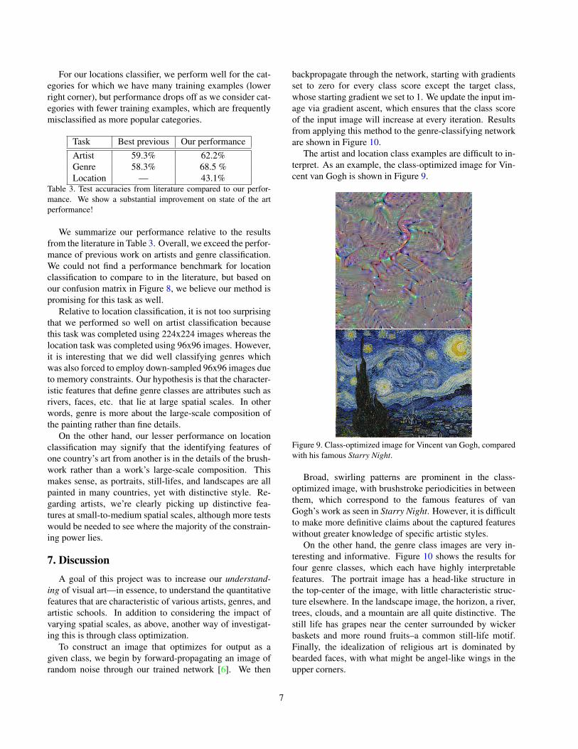
The artist and location class examples are difficult to in-terpret. As an example, the class-optimized image for Vin-cent van Gogh is shown in Figure 9.
Figure 9. Class-optimized image for Vincent van Gogh, comparedwith his famous Starry Night.
Broad, swirling patterns are prominent in the class-optimized image, with brushstroke periodicities in betweenthem, which correspond to the famous features of vanGogh’s work as seen in Starry Night. However, it is difficultto make more definitive claims about the captured featureswithout greater knowledge of specific artistic styles.
On the other hand, the genre class images are very in-teresting and informative. Figure 10 shows the results forfour genre classes, which each have highly interpretablefeatures. The portrait image has a head-like structure inthe top-center of the image, with little characteristic struc-ture elsewhere. In the landscape image, the horizon, a river,trees, clouds, and a mountain are all quite distinctive. Thestill life has grapes near the center surrounded by wickerbaskets and more round fruits–a common still-life motif.Finally, the idealization of religious art is dominated bybearded faces, with what might be angel-like wings in theupper corners.
7

Figure 10. Clockwise from top-left, images from the portrait, land-scape, religious, and still life class optimizations.
8. Conclusions and Future Work
After exploring our dataset and implementing three clas-sifiers, we obtain results that improve significantly on thestate of the art for artist and genre classification. Our resultsfrom analyzing images at varying spatial scales showed thatwhile artistic genre can be inferred from highly downsam-pled images, the location of origin is likely best constrainedby small-scale (brushstroke) information. In addition, weused class optimization to extract the quantitative featuresthat define various genres of art.
In this work, we were frequently limited by memory con-straints; it is clear that our next step in improving these re-sults is to circumvent this resource limitation. Loading thetraining images on-the-fly will allow our server to handleall the data we have available at maximum image resolu-tion. Although this I/O would introduce more overhead,the cost of the extra time needed for training should be off-set by the ability to use the larger image sizes, extractinginformation at all spatial scales, rather than the downsam-pled 224x224 or 96x96 pixel images. Furthermore, withthis on-the-fly loading, we would also be able to performdata augmentation to increase the number of effective train-ing examples. We believe these changes have the highestpotential for yielding significant gains.
References[1] L. Baraldi. https://gist.github.com/
baraldilorenzo/07d7802847aaad0a35d3.[2] F. Bastien, P. Lamblin, R. Pascanu, J. Bergstra, I. J. Good-
fellow, A. Bergeron, N. Bouchard, and Y. Bengio. Theano:new features and speed improvements. Deep Learning andUnsupervised Feature Learning NIPS 2012 Workshop, 2012.
[3] J. Bergstra and Y. Bengio. Random search for hyper-parameter optimization. Journal of Machine Learning Re-search, 13:281–305, Feb. 2012.
[4] J. Bergstra, O. Breuleux, F. Bastien, P. Lamblin, R. Pascanu,G. Desjardins, J. Turian, D. Warde-Farley, and Y. Bengio.Theano: a CPU and GPU math expression compiler. In Pro-ceedings of the Python for Scientific Computing Conference(SciPy), June 2010. Oral Presentation.
[5] H. Cai, Q. Wu, T. Corradi, and P. Hall. The Cross-DepictionProblem: Computer Vision Algorithms for Recognising Ob-jects in Artwork and in Photographs. ArXiv e-prints, May2015.
[6] F. Chollet. http://blog.keras.io/how-convolutional-neural-networks-see-the-world.html.
[7] F. Chollet. Keras. https://github.com/fchollet/keras, 2015.
[8] G. Didi-Huberman and A. F. Angelico. Fra Angelico: Dis-semblance Figuration. University of Chicago Press, 1995.
[9] P. DiMaggio. Classification in art. American SociologicalReview, 52(4):440–455, 1987.
[10] K. He, X. Zhang, S. Ren, and J. Sun. Spatial Pyramid Pool-ing in Deep Convolutional Networks for Visual Recognition.ArXiv e-prints, June 2014.
[11] K. He, X. Zhang, S. Ren, and J. Sun. Delving Deep into Rec-tifiers: Surpassing Human-Level Performance on ImageNetClassification. ArXiv e-prints, Feb. 2015.
[12] S. Ioffe and C. Szegedy. Batch Normalization: Accelerat-ing Deep Network Training by Reducing Internal CovariateShift. ArXiv e-prints, Feb. 2015.
[13] A. Kanazawa, A. Sharma, and D. Jacobs. Locally Scale-Invariant Convolutional Neural Networks. ArXiv e-prints,Dec. 2014.
[14] D. Kingma and J. Ba. Adam: A Method for Stochastic Opti-mization. ArXiv e-prints, Dec. 2014.
[15] T. Mensink and J. van Gemert. The rijksmuseum challenge:Museum-centered visual recognition. 2014.
[16] V. Nair and G. E. Hinton. Rectified linear units improve re-stricted boltzmann machines. In ICML, 2010.
[17] B. T. Polyak. Some methods of speeding up the convergenceof iteration methods. USSR Computational Mathematics andMathematical Physics, 4(5):1–17, 1964.
[18] B. Saleh, K. Abe, R. Singh Arora, and A. Elgammal. TowardAutomated Discovery of Artistic Influence. ArXiv e-prints,Aug. 2014.
[19] B. Saleh and A. Elgammal. Large-scale Classification ofFine-Art Paintings: Learning The Right Metric on The RightFeature. ArXiv e-prints, May 2015.
[20] K. Simonyan and A. Zisserman. Very deep convolu-tional networks for large-scale image recognition. CoRR,abs/1409.1556, 2014.
[21] E. L. Spratt and A. Elgammal. Computational Beauty: Aes-thetic Judgment at the Intersection of Art and Science. ArXive-prints, Sept. 2014.
8


