Download - The Winner’s Curse in Group Risk - Actuaries
The Winner’s Curse in Group Risk
Prepared by Colin Yellowlees
Presented to the Actuaries Institute
Actuaries Summit
20-21 May 2013
Sydney
This paper has been prepared for Actuaries Institute 2013 Actuaries Summit.
The Institute Council wishes it to be understood that opinions put forward herein are not necessarily those of the Institute and
the Council is not responsible for those opinions.
copyright Colin Yellowlees
The Institute will ensure that all reproductions of the paper acknowledge the Author/s as
the author/s, and include the above copyright statement.
Institute of Actuaries of Australia
ABN 69 000 423 656
Level 7, 4 Martin Place, Sydney NSW Australia 2000
t +61 (0) 2 9233 3466 f +61 (0) 2 9233 3446
e [email protected] w www.actuaries.asn.au
The Winner’s Curse in Group Risk
2
Abstract
The Winner’s Curse is a theory that in an auction there is a tendency for the winner to have
overpaid for the item purchased. This is especially the case where it is difficult to
determine the intrinsic value of an item and the item has a similar value to each bidder.
The Group Risk market in Australia appears to meet many of the requirements for the
Winner’s Curse to exist. Through the use of a simple model, this paper explores the
possible implications of the Winner’s Curse and discusses some associated issues.
Keywords: Winner’s Curse, Group Risk,
1 Introduction
“There are a lot of ways to lose money in insurance, and the industry
never ceases searching for new ones.” Warren Buffett
The aim of this paper is to use a particular subject, the Winner’s Curse, to bring together a
number of topics that have a strong bearing on both how Group Risk pricing is performed
and the way that it is gone about. The many ideas in this paper are far from original and
have been covered in much greater depth elsewhere; however, I believe that there is
significant value in bringing all of these ideas together: particularly, for those involved in
Group Risk pricing who may not have come across some of them before.
Partway through writing this paper, I realised that I had taken on a very challenging topic
and could not do it justice. I made the decision at the time that there would be more
value in bringing together as many ideas as possible rather than concentrating on one
area in particular; hence, much of this paper is still a work in progress.
The concepts discussed in this paper are focused more heavily toward large group risk
schemes that are generally priced with a heavy reliance on self-experience rating rather
than smaller group risk schemes that are mostly priced using book rates.
Finally, I would like to acknowledge the contributions of Darren Wickham and Saul Field
who have provided invaluable assistance along the way. Their advice has been greatly
appreciated and improved this paper immeasurably.
2 Summary
The insurance industry as a whole is extremely complex and it is generally actuaries with
our specialist skills who are heavily relied upon to ensure that insurance companies are
soundly run. In Group Risk, it is often the actuary who determines or recommends the
premium rates or price to be offered whenever a group risk scheme is up for renewal.
Often, the price will be determined through a tender process that involves a number of
competing insurers. Vital to this, is that the actuary needs to be aware of how the Group
Risk insurance market operates and the implications of this in determining the price.
The Winner’s Curse in Group Risk
3
The selection of an insurer for a Group Risk scheme is usually determined through a tender
process, which for larger schemes is conducted through a formal tender process often via
an advisor along with the issue of a Request For Proposal (RFP). In any tender, a large
weighting is usually given to the price offered by the competing insurers with the winning
insurer often having the lowest or close to the lowest price.
In a tender, each insurer will determine a price that has been determined from their best
estimate of the future claims cost based upon the historical claims information provided
by the tendering scheme or their advisor. The determination of a best estimate for future
claims can use a variety of methods and each insurer will use their own internal models,
taking into account a wide range of information and involving application of their own
judgement.
As pricing is carried out independently, no two best estimates determined by the
participating insurers will be the same; hence, the best estimates determined will comprise
a range of reasonable estimates. Assuming that each insurer’s best estimate of the future
claim costs is an unbiased estimate of the expected claim costs, then some of those
estimates would be below the expected claims cost and some would be above. If the
winning insurer has the lowest price, then we would expect that the winning insurer’s best
estimate would be below the expected claim costs all other things being equal.
Section 4 of this paper shows that with a few basic assumptions, a simple model can
demonstrate that the outcome of the situation where each insurer bases its price on its
own best estimate will result in the lowest best estimate being materially below the
expected mean claim costs; hence, the winning insurer pricing at too low a price.
The implication of this is that unless competing insurers take the Winner’s Curse into
consideration then, all other things being equal, the winning insurer is likely to have under -
priced.
The potential magnitude of the Winner’s Curse is partly determined by the likely range of
the best estimates from insurers. The range of best estimates depends on how accurately
insurers can estimate the expected claim costs. Section 5 discusses some of the causes
for possibly having a wide range of estimates. Section 6 raises some other issues that are
strongly related to the Winner’s Curse and will have a bearing on the extent of it.
Finally this paper examines why the Winner’s Curse may not have been evident in the past
and discusses how we should potentially respond to the implications of the Winner’s Curse
to ensure that we do not become “cursed” in the future.
3 Background and Reading
The Winner’s Curse as a concept was first described in a 1971 paper by Capen, Clapp
and Campbell (1971) in their paper “Competitive Bidding in High-Risk Situations” in the
context of the sale or auction of oil drilling rights. The background to the original idea is
The Winner’s Curse in Group Risk
4
simple: suppose that a number of parties are bidding for the drilling rights to a particular
parcel of land. If the rights are worth the same to each party, then the auction is a
common value auction and each party is trying to estimate the common value of the
land. Given the difficulty of valuing a parcel of land, some estimates are likely to be too
high and some estimates too low. The winner of the auction will be the party whose
estimate was too high and can be described as “cursed”.
Since that original paper, the Winner’s Curse has been studied in relation to auctions for
radio spectrums, book rights, market for free agents in baseball, takeovers and many
other areas. More recently, there have been papers specific to insurance.
A good starting point for anyone interested in this topic is Richard Thaler’s paper “The
Winner's Curse: Paradoxes and Anomalies of Economic Life”.
Other important papers which are specific to insurance and recommended further
reading are GIRO Working Party (2009), GRIT (2006) and Lewis et.al. (2005).
It should be noted that Lewis et.al. (2006) was the only paper that I found that related to
group risk business.
4 A simple model
One of the simplest ways to demonstrate the Winner’s Curse and explore its implications is
through the use of a simple model. We can assume that best estimates are unbiased
estimates of the true statistical mean, then model the outcomes from simulations of a
hypothetical tender to see the impact.
We first start with a model where all insurers can price the risks equally well, have the same
margins and where the lowest price wins.
4.1 Identical insurers
Consider a situation where we have a number of insurers all competing in a series of
tenders for identical Group Risk schemes. Assume that:
The current price of the scheme prior to each tender is 100
the true mean loss ratio for each scheme is 85% i.e. expected claim costs are 85
all insurers produce unbiased estimates of the true mean that are normally
distributed with a standard error of 10%
all insurers require a margin of 15% of the premium to meet profit margins and
expenses
the winner of each tender is the insurer with the lowest price
Running 1,000,000 simulations of the above scenario we get the following results:
The Winner’s Curse in Group Risk
5
Table 4.1 – Simple model of Winner’s Curse
Number of
Companies
Average Winning
Price
Expected Loss
Ratio on winning
price
Average Margin
1 100.03 84.97% 15.03%
2 94.38 90.07% 9.93%
3 91.56 92.84% 7.16%
4 89.72 94.73% 5.27%
5 88.38 96.17% 3.83%
6 87.32 97.34% 2.66%
7 86.49 98.28% 1.72%
8 85.77 99.10% 0.90%
The expected loss ratio above is based upon the new price so that if the price is below 100
then the loss ratio will be higher than 85% i.e. the winning price divided by 85.
The above table clearly demonstrates the main premise of the Winner’s Curse. That is, in
a market where participants price using best estimate loss ratios, then the expected long
term outcome will be worse than the best estimate.
It can also be clearly seen that as the number of participants increase, the expected loss
ratio increases and the average margin falls well below the 15% used by each company
for pricing.
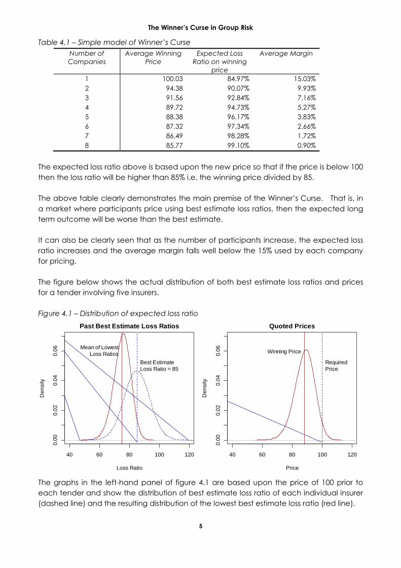
The figure below shows the actual distribution of both best estimate loss ratios and prices
for a tender involving five insurers.
Figure 4.1 – Distribution of expected loss ratio
The graphs in the left-hand panel of figure 4.1 are based upon the price of 100 prior to
each tender and show the distribution of best estimate loss ratio of each individual insurer
(dashed line) and the resulting distribution of the lowest best estimate loss ratio (red line).
40 60 80 100 120
0.0
00
.02
0.0
40
.06
Past Best Estimate Loss Ratios
Loss Ratio
De
nsity
Mean of Lowest
Loss Ratios
Best Estimate
Loss Ratio = 85
40 60 80 100 120
0.0
00
.02
0.0
40
.06
Quoted Prices
Price
De
nsity
Winning Price
Required
Price
The Winner’s Curse in Group Risk
6
The right-hand panel of figure 4.1 shows a graph of the expected winning price, which is
likely to be significantly below the required price of 100 to achieve a target margin of 15%.
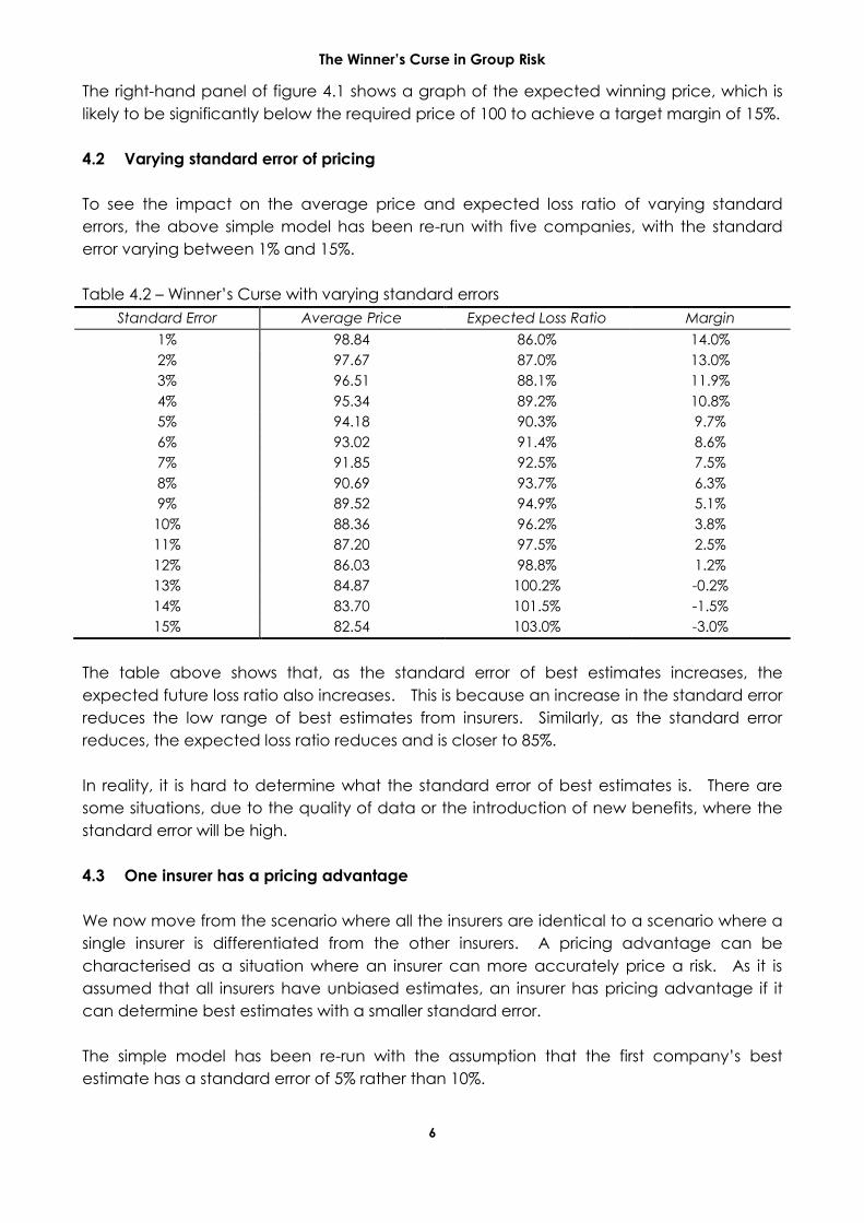
4.2 Varying standard error of pricing
To see the impact on the average price and expected loss ratio of varying standard
errors, the above simple model has been re-run with five companies, with the standard
error varying between 1% and 15%.
Table 4.2 – Winner’s Curse with varying standard errors
Standard Error Average Price Expected Loss Ratio Margin
1% 98.84 86.0% 14.0%
2% 97.67 87.0% 13.0%
3% 96.51 88.1% 11.9%
4% 95.34 89.2% 10.8%
5% 94.18 90.3% 9.7%
6% 93.02 91.4% 8.6%
7% 91.85 92.5% 7.5%
8% 90.69 93.7% 6.3%
9% 89.52 94.9% 5.1%
10% 88.36 96.2% 3.8%
11% 87.20 97.5% 2.5%
12% 86.03 98.8% 1.2%
13% 84.87 100.2% -0.2%
14% 83.70 101.5% -1.5%
15% 82.54 103.0% -3.0%
The table above shows that, as the standard error of best estimates increases, the
expected future loss ratio also increases. This is because an increase in the standard error
reduces the low range of best estimates from insurers. Similarly, as the standard error
reduces, the expected loss ratio reduces and is closer to 85%.
In reality, it is hard to determine what the standard error of best estimates is. There are
some situations, due to the quality of data or the introduction of new benefits, where the
standard error will be high.
4.3 One insurer has a pricing advantage
We now move from the scenario where all the insurers are identical to a scenario where a
single insurer is differentiated from the other insurers. A pricing advantage can be
characterised as a situation where an insurer can more accurately price a risk. As it is
assumed that all insurers have unbiased estimates, an insurer has pricing advantage if it
can determine best estimates with a smaller standard error.
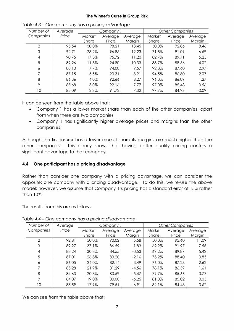
The simple model has been re-run with the assumption that the first company’s best
estimate has a standard error of 5% rather than 10%.
The Winner’s Curse in Group Risk
7
Table 4.3 – One company has a pricing advantage
Number of
Companies
Average
Price
Company 1 Other Companies
Market
Share
Average
Price
Average
Margin
Market
Share
Average
Price
Average
Margin
2 95.54 50.0% 98.21 13.45 50.0% 92.86 8.46
3 92.71 28.2% 96.85 12.23 71.8% 91.09 6.69
4 90.75 17.3% 95.72 11.20 82.7% 89.71 5.25
5 89.26 11.3% 94.80 10.33 88.7% 88.56 4.02
6 88.10 7.7% 94.00 9.57 92.3% 87.60 2.97
7 87.15 5.5% 93.31 8.91 94.5% 86.80 2.07
8 86.36 4.0% 92.66 8.27 96.0% 86.09 1.27
9 85.68 3.0% 92.16 7.77 97.0% 85.48 0.56
10 85.09 2.3% 91.72 7.32 97.7% 84.93 -0.09
It can be seen from the table above that:
Company 1 has a lower market share than each of the other companies, apart
from when there are two companies
Company 1 has significantly higher average prices and margins than the other
companies
Although the first insurer has a lower market share its margins are much higher than the
other companies. This clearly shows that having better quality pricing confers a
significant advantage to that company.
4.4 One participant has a pricing disadvantage
Rather than consider one company with a pricing advantage, we can consider the
opposite: one company with a pricing disadvantage. To do this, we re-use the above
model; however, we assume that Company 1’s pricing has a standard error of 15% rather
than 10%.
The results from this are as follows:
Table 4.4 – One company has a pricing disadvantage
Number of
Companies
Average
Price
Company 1 Other Companies
Market
Share
Average
Price
Average
Margin
Market
Share
Average
Price
Average
Margin
2 92.81 50.0% 90.02 5.58 50.0% 95.60 11.09
3 89.97 37.1% 86.59 1.83 62.9% 91.97 7.58
4 88.24 30.8% 84.55 -0.53 69.2% 89.87 5.42
5 87.01 26.8% 83.20 -2.16 73.2% 88.40 3.85
6 86.05 24.0% 82.14 -3.49 76.0% 87.28 2.62
7 85.28 21.9% 81.29 -4.56 78.1% 86.39 1.61
8 84.63 20.3% 80.59 -5.47 79.7% 85.66 0.77
9 84.07 19.0% 80.00 -6.25 81.0% 85.02 0.03
10 83.59 17.9% 79.51 -6.91 82.1% 84.48 -0.62
We can see from the table above that:
The Winner’s Curse in Group Risk
8
Company 1 has an average loss ratio of above 100% with as few as 3 companies
Company 1 maintains a higher market share than its competitors
This clearly demonstrates the disadvantages to a company of having pricing that is poorer
than its competitors.
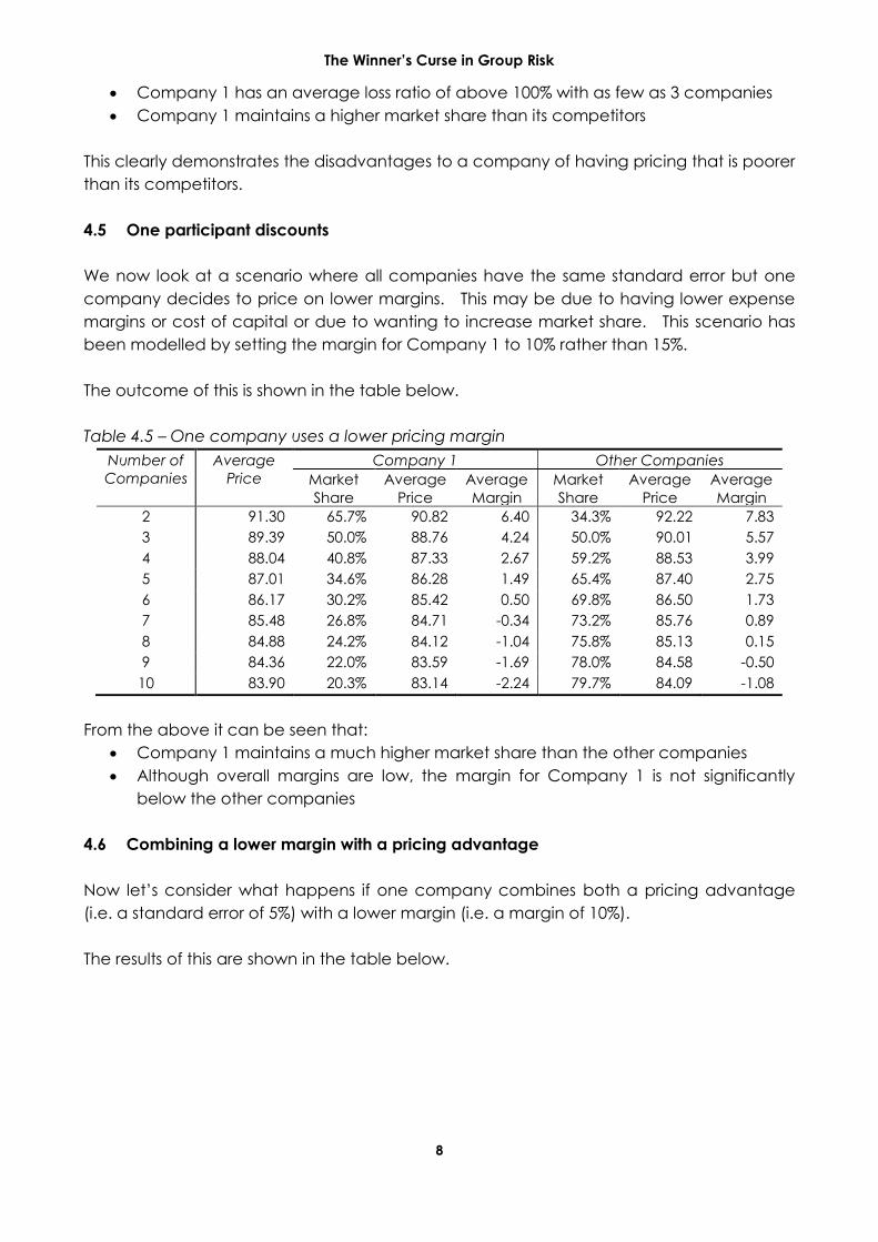
4.5 One participant discounts
We now look at a scenario where all companies have the same standard error but one
company decides to price on lower margins. This may be due to having lower expense
margins or cost of capital or due to wanting to increase market share. This scenario has
been modelled by setting the margin for Company 1 to 10% rather than 15%.
The outcome of this is shown in the table below.
Table 4.5 – One company uses a lower pricing margin
Number of
Companies
Average
Price
Company 1 Other Companies
Market
Share
Average
Price
Average
Margin
Market
Share
Average
Price
Average
Margin
2 91.30 65.7% 90.82 6.40 34.3% 92.22 7.83
3 89.39 50.0% 88.76 4.24 50.0% 90.01 5.57
4 88.04 40.8% 87.33 2.67 59.2% 88.53 3.99
5 87.01 34.6% 86.28 1.49 65.4% 87.40 2.75
6 86.17 30.2% 85.42 0.50 69.8% 86.50 1.73
7 85.48 26.8% 84.71 -0.34 73.2% 85.76 0.89
8 84.88 24.2% 84.12 -1.04 75.8% 85.13 0.15
9 84.36 22.0% 83.59 -1.69 78.0% 84.58 -0.50
10 83.90 20.3% 83.14 -2.24 79.7% 84.09 -1.08
From the above it can be seen that:
Company 1 maintains a much higher market share than the other companies
Although overall margins are low, the margin for Company 1 is not significantly
below the other companies
4.6 Combining a lower margin with a pricing advantage
Now let’s consider what happens if one company combines both a pricing advantage
(i.e. a standard error of 5%) with a lower margin (i.e. a margin of 10%).
The results of this are shown in the table below.
The Winner’s Curse in Group Risk
9
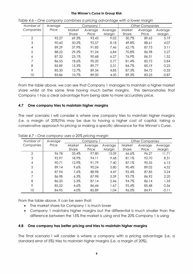
Table 4.6 – One company combines a pricing advantage with a lower margin
Number of
Companies
Average
Price
Company 1 Other Companies
Market
Share
Average
Price
Average
Margin
Market
Share
Average
Price
Average
Margin
2 92.27 69.3% 93.43 9.02 30.7% 89.65 5.19
3 90.60 50.2% 92.57 8.18 49.8% 88.61 4.07
4 89.29 37.9% 91.85 7.46 62.1% 87.73 3.11
5 88.22 29.2% 91.24 6.84 70.8% 86.98 2.27
6 87.32 23.1% 90.68 6.27 76.9% 86.31 1.52
7 86.55 18.6% 90.20 5.77 81.4% 85.72 0.84
8 85.89 15.3% 89.77 5.31 84.7% 85.19 0.23
9 85.30 12.7% 89.34 4.85 87.3% 84.72 -0.33
10 83.86 10.7% 89.00 4.50 89.3% 83.25 -0.87
From the table above, we can see that Company 1 manages to maintain a higher market
share whilst at the same time having much better margins. This demonstrates that
Company 1 has a clear advantage from being able to more accurately price.
4.7 One company tries to maintain higher margins
The next scenario I will consider is where one company tries to maintain higher margins
(i.e. a margin of 20%)This may be due to having a higher cost of capital, taking a
conservative approach to pricing or making a specific allowance for the Winner’s Curse.
Table 4.7 – One company uses a 20% pricing margin
Number of
Companies
Average
Price
Company 1 Other Companies
Market
Share
Average
Price
Average
Margin
Market
Share
Average
Price
Average
Margin
2 96.78 33.4% 97.80 13.09 66.6% 96.27 11.71
3 92.97 18.9% 94.11 9.68 81.1% 92.70 8.31
4 90.71 12.9% 91.79 7.40 87.1% 90.55 6.13
5 89.14 9.6% 90.24 5.80 90.4% 89.02 4.52
6 87.94 7.6% 88.98 4.47 92.4% 87.85 3.24
7 86.98 6.3% 87.98 3.39 93.7% 86.92 2.20
8 86.20 5.3% 87.14 2.46 94.7% 86.14 1.33
9 85.52 4.6% 86.44 1.67 95.4% 85.48 0.56
10 84.95 4.0% 85.89 1.04 96.0% 84.91 -0.11
From the table above, it can be seen that:
The market share for Company 1 is much lower
Company 1 maintains higher margins but the differential is much smaller than the
difference between the 15% the market is using and the 20% Company 1 is using
4.8 One company has better pricing and tries to maintain higher margins
The final scenario I will consider is where a company with a pricing advantage (i.e. a
standard error of 5%) tries to maintain higher margins (i.e. a margin of 20%).
The Winner’s Curse in Group Risk
10
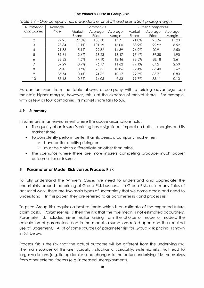
Table 4.8 – One company has a standard error of 5% and uses a 20% pricing margin
Number of
Companies
Average
Price
Company 1 Other Companies
Market
Share
Average
Price
Average
Margin
Market
Share
Average
Price
Average
Margin
2 97.95 29.0% 103.30 17.71 71.0% 95.76 11.23
3 93.84 11.1% 101.19 16.00 88.9% 92.92 8.52
4 91.35 5.1% 99.52 14.59 94.9% 90.91 6.50
5 89.61 2.6% 98.23 13.47 97.4% 89.38 4.90
6 88.32 1.5% 97.10 12.46 98.5% 88.18 3.61
7 87.29 0.9% 96.17 11.62 99.1% 87.21 2.53
8 86.45 0.6% 95.35 10.86 99.4% 86.40 1.62
9 85.74 0.4% 94.62 10.17 99.6% 85.71 0.83
10 85.13 0.3% 94.05 9.63 99.7% 85.11 0.13
As can be seen from the table above, a company with a pricing advantage can
maintain higher margins; however, this is at the expense of market share. For example,
with as few as four companies, its market share falls to 5%.
4.9 Summary
In summary, in an environment where the above assumptions hold:
The quality of an insurer’s pricing has a significant impact on both its margins and its
market share
To consistently perform better than its peers, a company must either:
o have better quality pricing; or
o must be able to differentiate on other than price.
The scenarios where there are more insurers competing produce much poorer
outcomes for all insurers
5 Parameter or Model Risk versus Process Risk
To fully understand the Winner’s Curse, we need to understand and appreciate the
uncertainty around the pricing of Group Risk business. In Group Risk, as in many fields of
actuarial work, there are two main types of uncertainty that we come across and need to
understand. In this paper, they are referred to as parameter risk and process risk.
To price Group Risk requires a best estimate which is an estimate of the expected future
claim costs. Parameter risk is then the risk that the true mean is not estimated accurately.
Parameter risk includes mis-estimation arising from the choice of model or models, the
calculation of parameters used in the model, assumptions relied upon and the required
use of judgement. A list of some sources of parameter risk for Group Risk pricing is shown
in 5.1 below.
Process risk is the risk that the actual outcome will be different from the underlying risk.
The main sources of this are typically : stochastic variability, systemic risks that lead to
larger variations (e.g. flu epidemics) and changes to the actual underlying risks themselves
from other external factors (e.g. increased unemployment).
The Winner’s Curse in Group Risk
11
GRIT [2006] provides an excellent description of the parameter risk and process risk in the
context of actuarial work.
A situation where many of us will have recently encountered both parameter risk and
process risk is with regards to LAGIC. In LPS115, the future stress margin in a large part
covers the parameter risk of the estimated liabilities whereas the random stress margin is
required to cover the process risk.
As parameter risk is the risk that the best estimate does not accurately estimate the true
mean, it is parameter risk that is relevant when considering the extent of the Winner’s
Curse.
5.1 Pricing Methodology
To fully understand the parameter risk associated with Group Risk pricing requires an
understanding of how group insurance business is priced. Although there will be
variations between insurers, the methodology will largely follow the same main steps.
These steps are:
1. Estimate what the past claims experience has been
2. Adjust the past claims experience to how we believe it will perform in the future
3. Determine how much weight or credibility to give this estimate and blend it with
the insurers own internal basis
4. Add loadings for expenses, reinsurance, cost of profit shares, profit and/or cost
of capital
Some insurers may perform steps 2 and 3 in reverse order.
All of the above steps are subject to parameter risk with some of the specific sources
being:
interpretation of data
choice of the experience period
segmentation of data
credibility formula to blend with an insurers book or risk rates
the book or risk rates themselves
IBNR methodology e.g. to use amounts v claim counts, choice of time interval
tail factors
use of subjective information
allowance for product changes
costing of profit shares
The list of all items that contribute to parameter risk is long; hence, the above list is not
exhaustive.

The Winner’s Curse in Group Risk
12
5.2 Can we quantify parameter risk?
Within the actuarial profession, we use the term “best estimate” to refer to the estimate of
the mean of possible outcomes. Although the best estimate is a point estimate the best
estimate is often only one estimate from a range of reasonable estimates.
To measure the parameter uncertainty in the best estimate is difficult and a number of
possible methods could be adopted to provide some guide as to what a reasonable
range of this variable could be. Some possible methods are:
Carry out a study of how pricing estimates have varied from eventual outcomes.
This could be achieved by either comparing the estimates of past claim costs or
the estimates of future claim costs
Perform a comparison of price estimates across multiple insurers
Build a bottom-up view of parameter risk by quantifying the potential error from
various elements of the price
To give some insight into the possible ranges, 5.3 below summarises the surprising results of
Blumsohn (2009) which describes a survey on IBNR estimates that tabulated a very wide
range of estimates. Section 5.4 considers a bottom-up approach by looking at few of the
model choices that would need to be made in pricing.
In addition, many insurers will have recently determined their margins for LAGIC and
pricing actuaries could look to build on this to arrive at a view of their own parameter risk.
5.3 Empirical evidence
Most pricing actuaries work within individual companies and so will only have a limited
view of the range of prices produced for individual tenders; hence, they are unable to
build a full view of prices in the market. Each individuals experience is generally limited to
the feedback that is provided during tenders and the range of prices provided by
reinsurers.
One paper available that provides some evidence as to how independent views can vary
is Blumsohn and Laufer (2009). In this paper, the authors surveyed 52 General Insurance
actuaries, requesting them each to provide an estimate of the IBNR from a sample set of
data covering 10 years of observed experience. The results of this paper showed that the
IBNR estimates provided by the surveyed actuaries for the 10-year period had a standard
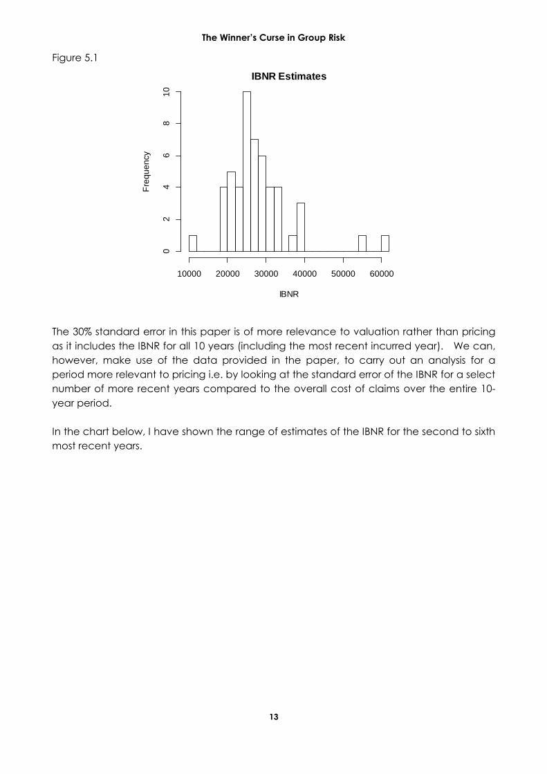
error of 30%. The figure below shows a histogram of the IBNR estimates in their paper.
The Winner’s Curse in Group Risk
13
Figure 5.1
The 30% standard error in this paper is of more relevance to valuation rather than pricing
as it includes the IBNR for all 10 years (including the most recent incurred year). We can,
however, make use of the data provided in the paper, to carry out an analysis for a
period more relevant to pricing i.e. by looking at the standard error of the IBNR for a select
number of more recent years compared to the overall cost of claims over the entire 10-
year period.
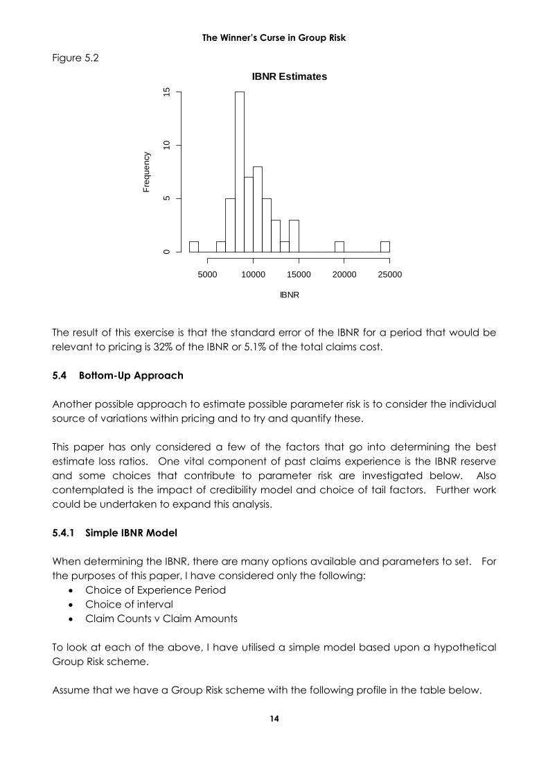
In the chart below, I have shown the range of estimates of the IBNR for the second to sixth
most recent years.
IBNR Estimates
IBNR
Fre
qu
en
cy
10000 20000 30000 40000 50000 60000
02
46
81
0
The Winner’s Curse in Group Risk
14
Figure 5.2
The result of this exercise is that the standard error of the IBNR for a period that would be
relevant to pricing is 32% of the IBNR or 5.1% of the total claims cost.
5.4 Bottom-Up Approach
Another possible approach to estimate possible parameter risk is to consider the individual
source of variations within pricing and to try and quantify these.
This paper has only considered a few of the factors that go into determining the best
estimate loss ratios. One vital component of past claims experience is the IBNR reserve
and some choices that contribute to parameter risk are investigated below. Also
contemplated is the impact of credibility model and choice of tail factors. Further work
could be undertaken to expand this analysis.
5.4.1 Simple IBNR Model
When determining the IBNR, there are many options available and parameters to set. For
the purposes of this paper, I have considered only the following:
Choice of Experience Period
Choice of interval
Claim Counts v Claim Amounts
To look at each of the above, I have utilised a simple model based upon a hypothetical
Group Risk scheme.
Assume that we have a Group Risk scheme with the following profile in the table below.
IBNR Estimates
IBNR
Fre
qu
en
cy
5000 10000 15000 20000 25000
05
10
15

The Winner’s Curse in Group Risk
15
Table 5.1
Age Band Number of Lives Sum Insured Annual Claim Rate
20-29 20,000 100,000 0.0005
30-39 25,000 70,000 0.0007
40-49 30,000 40,000 0.0014
50-59 20,000 20,000 0.0040
60-69 5,000 10,000 0.0060
For this scheme we assume that:
Claims are incurred evenly throughout each annual period
Claim delays are distributed according to a gamma distribution
Using the above scheme profile, we can run a number of simulations to produce incurred
claims and notified claims. Using the notified claims, we can then calculate the IBNR
using the basic chain-ladder method. By slightly varying the application of the basic
chain-ladder method to the notified claims, we can then compare the results to each
other and to the total incurred claims. This then provides a simple demonstration of how
the result changes to variations in the model or the parameters.
5.4.2 Choice of period
In Group Risk pricing, one of the most important and difficult decisions is choosing the past
exposure period upon which to base the rest of the pricing on. This is often an exercise in
trying to find a balance between:
including more recent periods where the final cost of claims is still very uncertain;
and
including older periods from which the underlying experience may have changed
and is less relevant to the future; and
including a sufficiently long period of time to maximise the amount of credibility
from the schemes own experience.
Using the above example scheme, 10,000 simulations were run to generate the number of
notified claims for a 10-year exposure period. From the notified claims, the total number
of reported claims and IBNR claims were calculated for each of the 10 exposure years.
This IBNR was calculated using the basic chain-ladder method without any adjustments.
The results of this model are shown in the table below with year 10 being the most recent
year of exposure.
The Winner’s Curse in Group Risk
16
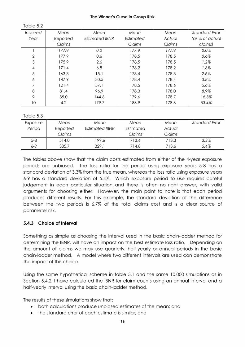
Table 5.2
Incurred
Year
Mean
Reported
Claims
Mean
Estimated IBNR
Mean
Estimated
Claims
Mean
Actual
Claims
Standard Error
(as % of actual
claims)
1 177.9 0.0 177.9 177.9 0.0%
2 177.9 0.6 178.5 178.5 0.6%
3 175.9 2.6 178.5 178.5 1.2%
4 171.4 6.8 178.2 178.2 1.8%
5 163.3 15.1 178.4 178.3 2.6%
6 147.9 30.5 178.4 178.4 3.8%
7 121.4 57.1 178.5 178.6 5.6%
8 81.4 96.9 178.3 178.0 8.9%
9 35.0 144.6 179.6 178.7 16.3%
10 4.2 179.7 183.9 178.3 53.4%
Table 5.3
Exposure
Period
Mean
Reported
Claims
Mean
Estimated IBNR
Mean
Estimated
Claims
Mean
Actual
Claims
Standard Error
5-8 514.0 199.6 713.6 713.3 3.3%
6-9 385.7 329.1 714.8 713.6 5.4%
The tables above show that the claim costs estimated from either of the 4-year exposure
periods are unbiased. The loss ratio for the period using exposure years 5-8 has a
standard deviation of 3.3% from the true mean, whereas the loss ratio using exposure years
6-9 has a standard deviation of 5.4%. Which exposure period to use requires careful
judgement in each particular situation and there is often no right answer, with valid
arguments for choosing either. However, the main point to note is that each period
produces different results. For this example, the standard deviation of the difference
between the two periods is 6.7% of the total claims cost and is a clear source of
parameter risk.
5.4.3 Choice of Interval
Something as simple as choosing the interval used in the basic chain-ladder method for
determining the IBNR, will have an impact on the best estimate loss ratio. Depending on
the amount of claims we may use quarterly, half-yearly or annual periods in the basic
chain-ladder method. A model where two different intervals are used can demonstrate
the impact of this choice.
Using the same hypothetical scheme in table 5.1 and the same 10,000 simulations as in
Section 5.4.2, I have calculated the IBNR for claim counts using an annual interval and a
half-yearly interval using the basic chain-ladder method.
The results of these simulations show that:
both calculations produce unbiased estimates of the mean; and
the standard error of each estimate is similar; and
The Winner’s Curse in Group Risk
17
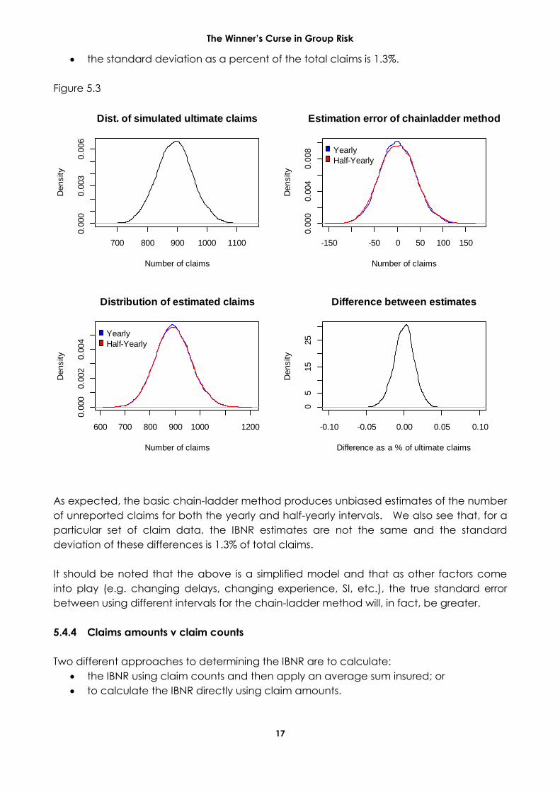
the standard deviation as a percent of the total claims is 1.3%.
Figure 5.3
As expected, the basic chain-ladder method produces unbiased estimates of the number
of unreported claims for both the yearly and half-yearly intervals. We also see that, for a
particular set of claim data, the IBNR estimates are not the same and the standard
deviation of these differences is 1.3% of total claims.
It should be noted that the above is a simplified model and that as other factors come
into play (e.g. changing delays, changing experience, SI, etc.), the true standard error
between using different intervals for the chain-ladder method will, in fact, be greater.
5.4.4 Claims amounts v claim counts
Two different approaches to determining the IBNR are to calculate:
the IBNR using claim counts and then apply an average sum insured; or
to calculate the IBNR directly using claim amounts.
700 800 900 1000 1100
0.0
00
0.0
03
0.0
06
Dist. of simulated ultimate claims
Number of claims
Density
600 700 800 900 1000 1200
0.0
00
0.0
02
0.0
04
Distribution of estimated claims
Number of claims
Density
Yearly
Half-Yearly
-150 -50 0 50 100 150
0.0
00
0.0
04
0.0
08
Estimation error of chainladder method
Number of claims
Density
Yearly
Half-Yearly
-0.10 -0.05 0.00 0.05 0.10
05
15
25
Difference between estimates
Difference as a % of ultimate claims
Density
The Winner’s Curse in Group Risk
18
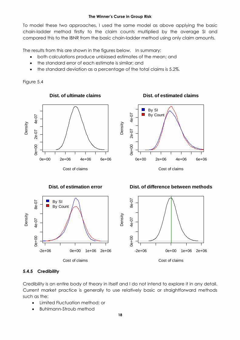
To model these two approaches, I used the same model as above applying the basic
chain-ladder method firstly to the claim counts multiplied by the average SI and
compared this to the IBNR from the basic chain-ladder method using only claim amounts.
The results from this are shown in the figures below. In summary:
both calculations produce unbiased estimates of the mean; and
the standard error of each estimate is similar; and
the standard deviation as a percentage of the total claims is 5.2%.
Figure 5.4
5.4.5 Credibility
Credibility is an entire body of theory in itself and I do not intend to explore it in any detail.
Current market practice is generally to use relatively basic or straightforward methods
such as the:
Limited Fluctuation method; or
Buhlmann-Stroub method
0e+00 2e+06 4e+06 6e+06
0e+
00
2e-0
74e-0
7
Dist. of ultimate claims
Cost of claims
Density
0e+00 2e+06 4e+06 6e+06
0e+
00
2e-0
74e-0
7
Dist. of estimated claims
Cost of claims
Density
By SI
By Count
-2e+06 0e+00 1e+06 2e+06
0e+
00
4e-0
78e-0
7
Dist. of estimation error
Cost of claims
Density
By SI
By Count
-2e+06 0e+00 1e+06 2e+06
0e+
00
4e-0
78e-0
7
Dist. of difference between methods
Cost of claims
Density
The Winner’s Curse in Group Risk
19
Each method will give a different weighting to experience and a company’s own book
rates. The choice of the method used will have a significant bearing on the final best
estimate determined.
5.4.6 Tail Factors
Determining tail factors is an area that requires a considerable amount of judgement by
the pricing actuary and there are many ways of dealing with this. Common methods
(which may be combined) are:
use the development pattern from other funds where more experience is available;
or
fit a distribution to the delay pattern that has been observed; or
assume a standard run-off pattern; or
assume that the data is fully developed (i.e. ignore it)
For TPD benefits, this is particularly important as claims can be reported with delays as long
as 10 years or more after the date of disability, furthermore, it is not often that 10 years of
claims data is available. Other complicating factors are:
the increasing prevalence of lawyers; and/or
experience is often not credible in the tail; and/or
changes in claim reporting patterns over time: claim delays vary over time and the
delays from claims incurred a number of years ago will be different from the claims
incurred today for example due to streamlining of company or fund reporting
processes.
The calculated tail factors can have a material contribution to the final best estimate and
a significant impact on overall parameter risk.
5.4.7 Summary
The above sections cover only a few of different aspects of determining the best estimate
and as discussed there are many options and choices to make in getting there. These
choices range from a simple choice of methodology to the more subjective application
of judgement and each choice has an impact on the final best estimate.
A useful way to consider these choices is as a number of random movements away from
the true mean. If, for example, we have 10 independent pricing factors that each have
a possible ±2% impact on the loss ratio then our parameter uncertainty would have a
standard error of approximately 6.2% (i.e. ~ 4 x (10 x 0.5 x 0.5)). As each of the identified
issues above are greater than 1%, it is very easy to see how the standard error could be as
great as 10% as was used throughout Section 4.
As a price is built up from a large number of choices that are made in pricing, a
reasonable assumption to make is that an individual best estimate is distributed normally
about the true mean.
The Winner’s Curse in Group Risk
20
For further reading that also looks into the issues surrounding parameter risk, I would
suggest the excellent paper by Lewis et.al. (2005); this paper provides a very good
discussion of many of the issues relating to Group Risk pricing.
6 Other factors to consider
So far we have assumed that both best estimates and prices are unbiased i.e. they are
neither systematically too high or too low. This is not necessarily the case and we should
consider what factors may lead to loss ratios and prices being biased.
In this paper, I have considered the following four factors that may lead to biased prices.
These are:
cognitive biases
third party pressures
market dynamics
operational risk
6.1 Cognitive biases
A cognitive bias is any of a wide range of errors in decision-making arising from the way
that people handle and process information. Cognitive biases are mostly sub-conscious;
hence, everybody is subject to cognitive biases to some degree. This paper will only
mention a few of the many cognitive biases that are particularly relevant to this topic.
6.1.1 Overconfidence
Much research has been carried out on tasks that involve judgement and decision-
making and there is much evidence to show that people tend to overestimate their own
abilities and skills. This conclusion holds whether or not it involves an area where people
have no particular skill in or professionals operating in their own field. Taylor (2000) states:
“The conclusion from all the research is that overconfidence is greatest for difficult tasks,
for forecasts with low predictability and for undertakings lacking fast, clear feedback.
Unfortunately, much actuarial work satisfies all three conditions!”
Unfortunately, this means that pricing actuaries are likely to trust in their abilities much
more than they should. If pricing actuaries were to be surveyed on how close they think
their best estimates were to the true mean, then as a group, they would likely
overestimate how close they were.
Much research has been carried out on the performance of experts in various fields and
the conclusions are that there have been many cases found where experts perform worse
than simple deterministic models.
6.1.2 Anchoring
The Winner’s Curse in Group Risk
21
Anchoring is where the availability of initial information subsequently influences future
decisions, even if little or no credibility is later placed on that information. Experiments
have shown that the effects of anchoring are extremely hard to ignore and that even the
introduction of absurd anchors have an influencing effect (Kahneman (2011)).
Within Group Risk pricing we can be influenced by many anchors of which the most
important is the current price. The pricing actuary needs to be conscious of the effect
that an anchor can have.
6.1.3 Confirmation Bias
Confirmation bias is the tendency for people to favour information that supports their own
position or desired outcome. This comes into play in a few different ways in pricing:
A tendency to only search for evidence that supports the position we prefer to
take. For example, if we are trying to justify a reduction in price, then we are more
likely to look for information to support a price reduction and less likely to search for
information that would lead to an upward revision;
A tendency to place more weight on information and evidence that supports the
position that we prefer to take. For example, if the recent experience of a scheme
has been good we may try and justify placing more weight on that experience.
The danger of the above should be clear to all. If we are looking for evidence that
supports a particular position, then we are more likely to find it and may not find
information that supports the opposite position irrespective of how valid it may be.
6.2 Third Party Pressure
Whilst third party influences can be wide ranging, most of them are quite subtle. We are all
familiar with the usual pressures that may be applied by parts of our business to provide
the best price possible and hence maximise the likelihood of winning e.g. to be more
aggressive and cut margins. Most of us are prepared for this and are more than capable
of dealing with these pressures.
However, some of the dangers that are less obvious that need to be considered are:
Are we only looking for evidence that will reduce the price? Are we increasing the
likelihood that we will find evidence that reduces the price over evidence that
increases the price?
How do we react to information that will increase the price - do we give it equal or
less weight?
Is any evidence that will increase the price being withheld by third parties?
Do we ultimately end up being more optimistic and end up being unconsciously
influenced anyway?
Where judgement is required, who do we discuss this with? Are these people
sufficiently independent and unbiased?

The Winner’s Curse in Group Risk
22
In pricing, there are a lot of choices to be made around assumptions. How can
we be sure that we are not subconsciously introducing some bias – either through
resisting the urging of being conservative or being influenced and being too
aggressive?
6.3 Market Dynamics
There are features of the Group Risk market that are different from a straightforward
common value auction that should be considered. Some of these are:
the information asymmetry between the various parties i.e. the incumbent insurer,
advisors, the fund itself and other participants in the market; and
the tiered nature of the market with the existence of reinsurers; and
the in-built options of many contracts have with the ability of the fund to retender
when it wants; and
the fact that some tenders have more than one round which can be either formal
or informal.
Most of the above factors will likely have a downward influence on price. The main
exception to this is: that it is generally in the interests of the incumbent insurer to release
information that will result in a higher price.
6.4 Operational Risk
If an insurer makes an error in their pricing that results in too low a price, then this may
result in them winning the scheme and incurring losses. Many tenders are complex and
not all the same.
Most companies will rely upon the use of spreadsheets to perform much of their pricing.
Spreadsheets are notoriously difficult to audit and check, so how confident are you that
your spreadsheets are error free? Research performed by specialists in this field (Panko
(2013)) has found that the majority of complex spreadsheets contain some sort of error.
This is another area where there is a danger of being overconfident and we need to
ensure that we have sufficiently robust processes in place.
7 Is there any evidence and if not why not?
Without any true evidence of the Winner’s Curse, the above discussions could be viewed
as being little more than theoretical. If the Winner’s Curse does exist then we may expect
to have seen losses by writers of Group Risk business. This section takes a brief look at the
results for Group Risk business as reported by APRA and then goes on to discuss reasons
that may counter the Winner’s Curse and why we may not be seeing losses.
7.1 APRA stats
The profitability of Group Risk business has been available from APRA since 2008. A
summary of the quarterly results since then are shown below.
The Winner’s Curse in Group Risk
23
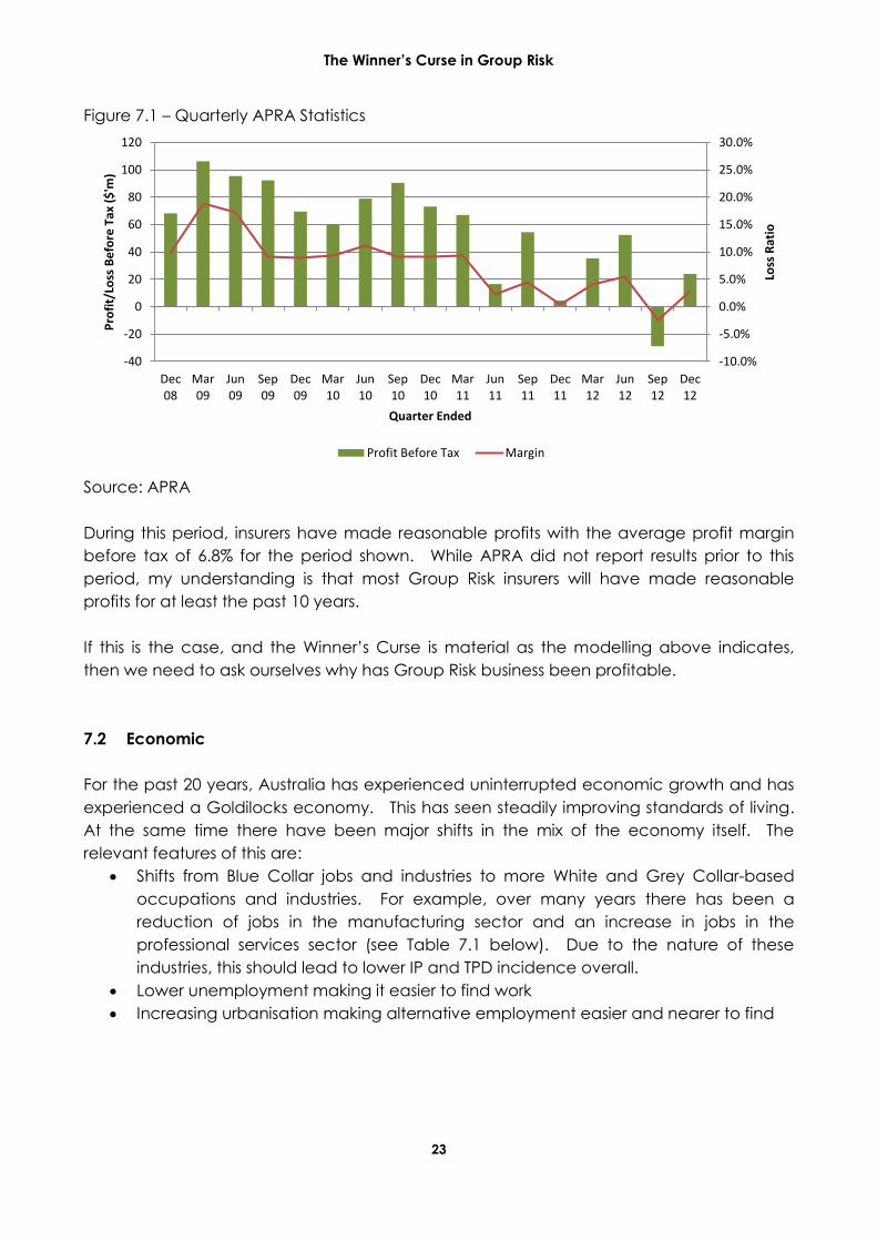
Figure 7.1 – Quarterly APRA Statistics
Source: APRA
During this period, insurers have made reasonable profits with the average profit margin
before tax of 6.8% for the period shown. While APRA did not report results prior to this
period, my understanding is that most Group Risk insurers will have made reasonable
profits for at least the past 10 years.
If this is the case, and the Winner’s Curse is material as the modelling above indicates,
then we need to ask ourselves why has Group Risk business been profitable.
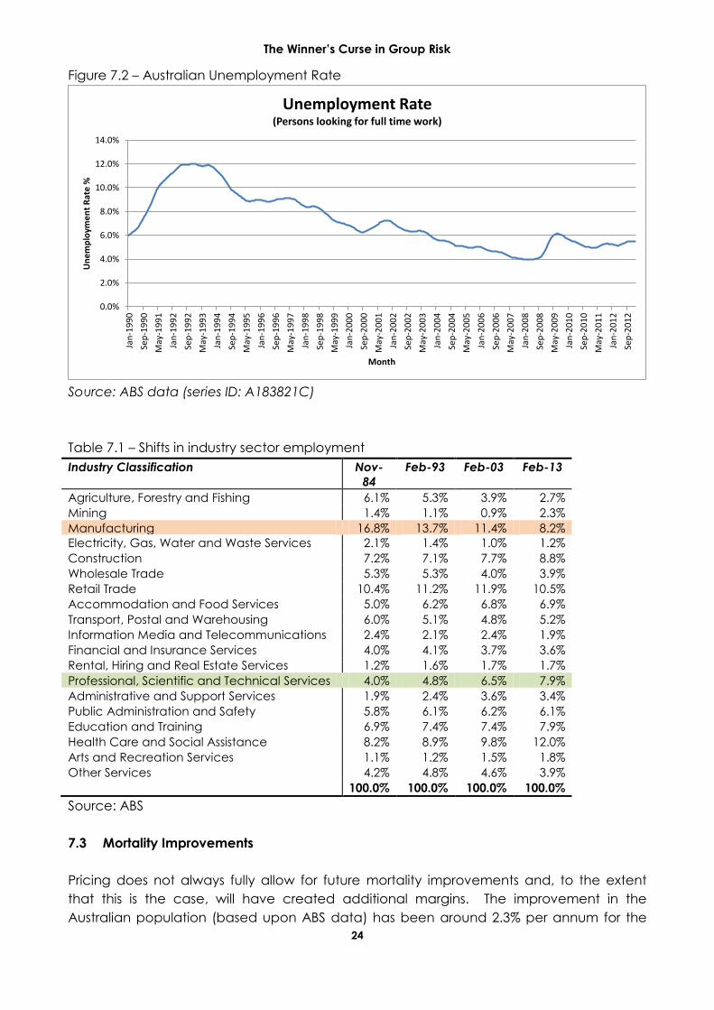
7.2 Economic
For the past 20 years, Australia has experienced uninterrupted economic growth and has
experienced a Goldilocks economy. This has seen steadily improving standards of living.
At the same time there have been major shifts in the mix of the economy itself. The
relevant features of this are:
Shifts from Blue Collar jobs and industries to more White and Grey Collar-based
occupations and industries. For example, over many years there has been a
reduction of jobs in the manufacturing sector and an increase in jobs in the
professional services sector (see Table 7.1 below). Due to the nature of these
industries, this should lead to lower IP and TPD incidence overall.
Lower unemployment making it easier to find work
Increasing urbanisation making alternative employment easier and nearer to find
-10.0%
-5.0%
0.0%
5.0%
10.0%
15.0%
20.0%
25.0%
30.0%
-40
-20
0
20
40
60
80
100
120
Dec08
Mar09
Jun09
Sep09
Dec09
Mar10
Jun10
Sep10
Dec10
Mar11
Jun11
Sep11
Dec11
Mar12
Jun12
Sep12
Dec12
Loss
Rat
io
Pro
fit/
Loss
Be
fore
Tax
($
'm)
Quarter Ended
Profit Before Tax Margin
The Winner’s Curse in Group Risk
24
Figure 7.2 – Australian Unemployment Rate
Source: ABS data (series ID: A183821C)
Table 7.1 – Shifts in industry sector employment
Industry Classification Nov-
84
Feb-93 Feb-03 Feb-13
Agriculture, Forestry and Fishing 6.1% 5.3% 3.9% 2.7%
Mining 1.4% 1.1% 0.9% 2.3%
Manufacturing 16.8% 13.7% 11.4% 8.2%
Electricity, Gas, Water and Waste Services 2.1% 1.4% 1.0% 1.2%
Construction 7.2% 7.1% 7.7% 8.8%
Wholesale Trade 5.3% 5.3% 4.0% 3.9%
Retail Trade 10.4% 11.2% 11.9% 10.5%
Accommodation and Food Services 5.0% 6.2% 6.8% 6.9%
Transport, Postal and Warehousing 6.0% 5.1% 4.8% 5.2%
Information Media and Telecommunications 2.4% 2.1% 2.4% 1.9%
Financial and Insurance Services 4.0% 4.1% 3.7% 3.6%
Rental, Hiring and Real Estate Services 1.2% 1.6% 1.7% 1.7%
Professional, Scientific and Technical Services 4.0% 4.8% 6.5% 7.9%
Administrative and Support Services 1.9% 2.4% 3.6% 3.4%
Public Administration and Safety 5.8% 6.1% 6.2% 6.1%
Education and Training 6.9% 7.4% 7.4% 7.9%
Health Care and Social Assistance 8.2% 8.9% 9.8% 12.0%
Arts and Recreation Services 1.1% 1.2% 1.5% 1.8%
Other Services 4.2% 4.8% 4.6% 3.9%
100.0% 100.0% 100.0% 100.0%
Source: ABS
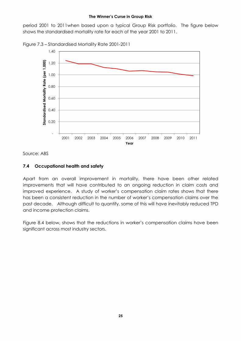
7.3 Mortality Improvements
Pricing does not always fully allow for future mortality improvements and, to the extent
that this is the case, will have created additional margins. The improvement in the
Australian population (based upon ABS data) has been around 2.3% per annum for the
0.0%
2.0%
4.0%
6.0%
8.0%
10.0%
12.0%
14.0%
Jan
-19
90
Sep
-19
90
May
-19
91
Jan
-19
92
Sep
-19
92
May
-19
93
Jan
-19
94
Sep
-19
94
May
-19
95
Jan
-19
96
Sep
-19
96
May
-19
97
Jan
-19
98
Sep
-19
98
May
-19
99
Jan
-20
00
Sep
-20
00
May
-20
01
Jan
-20
02
Sep
-20
02
May
-20
03
Jan
-20
04
Sep
-20
04
May
-20
05
Jan
-20
06
Sep
-20
06
May
-20
07
Jan
-20
08
Sep
-20
08
May
-20
09
Jan
-20
10
Sep
-20
10
May
-20
11
Jan
-20
12
Sep
-20
12
Un
em
plo
yme
nt
Rat
e %
Month
Unemployment Rate(Persons looking for full time work)
The Winner’s Curse in Group Risk
25
period 2001 to 2011when based upon a typical Group Risk portfolio. The figure below
shows the standardised mortality rate for each of the year 2001 to 2011.
Figure 7.3 – Standardised Mortality Rate 2001-2011
Source: ABS
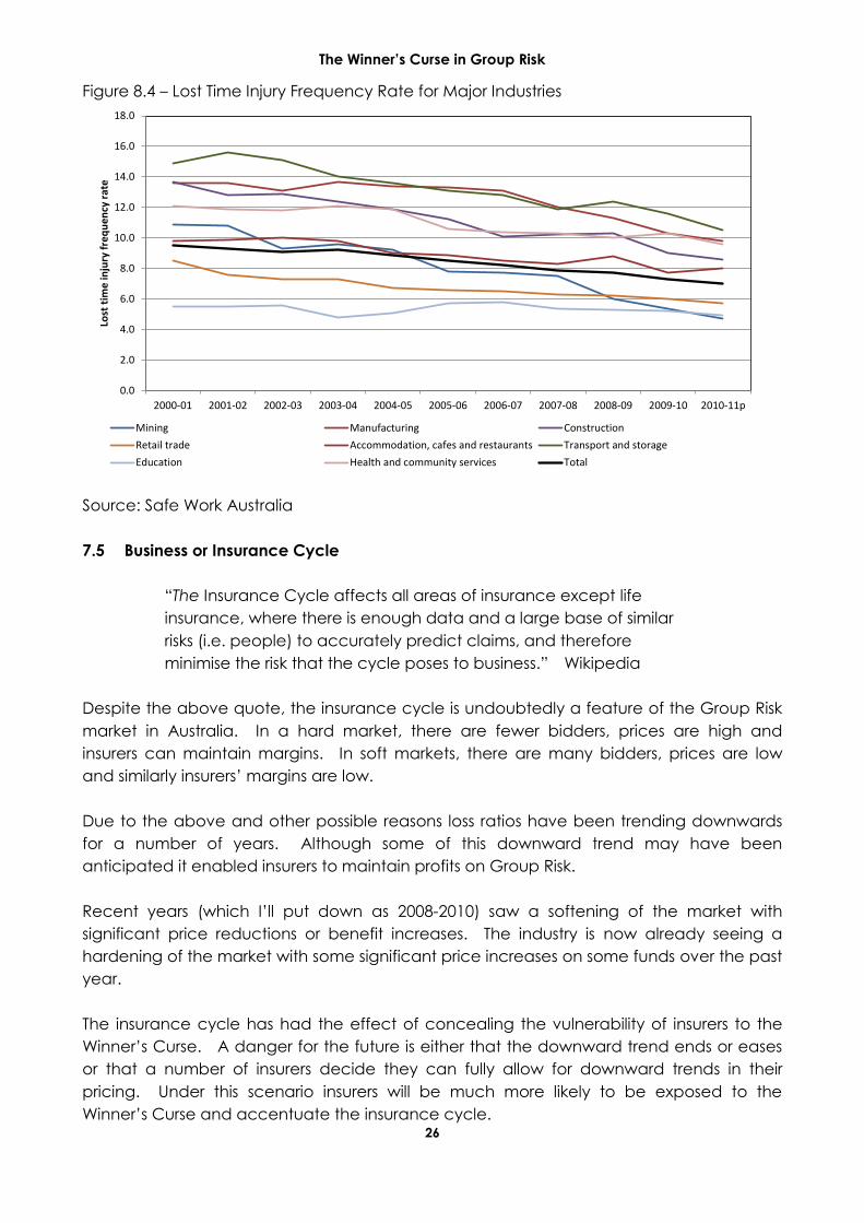
7.4 Occupational health and safety
Apart from an overall improvement in mortality, there have been other related
improvements that will have contributed to an ongoing reduction in claim costs and
improved experience. A study of worker’s compensation claim rates shows that there
has been a consistent reduction in the number of worker’s compensation claims over the
past decade. Although difficult to quantify, some of this will have inevitably reduced TPD
and income protection claims.
Figure 8.4 below, shows that the reductions in worker’s compensation claims have been
significant across most industry sectors.
-
0.20
0.40
0.60
0.80
1.00
1.20
1.40
2001 2002 2003 2004 2005 2006 2007 2008 2009 2010 2011
Sta
nd
ard
ise
d M
ort
ality
Ra
te (
pe
r 1,0
00)
Year
The Winner’s Curse in Group Risk
26
Figure 8.4 – Lost Time Injury Frequency Rate for Major Industries
Source: Safe Work Australia
7.5 Business or Insurance Cycle
“The Insurance Cycle affects all areas of insurance except life
insurance, where there is enough data and a large base of similar
risks (i.e. people) to accurately predict claims, and therefore
minimise the risk that the cycle poses to business.” Wikipedia
Despite the above quote, the insurance cycle is undoubtedly a feature of the Group Risk
market in Australia. In a hard market, there are fewer bidders, prices are high and
insurers can maintain margins. In soft markets, there are many bidders, prices are low
and similarly insurers’ margins are low.
Due to the above and other possible reasons loss ratios have been trending downwards
for a number of years. Although some of this downward trend may have been
anticipated it enabled insurers to maintain profits on Group Risk.
Recent years (which I’ll put down as 2008-2010) saw a softening of the market with
significant price reductions or benefit increases. The industry is now already seeing a
hardening of the market with some significant price increases on some funds over the past
year.
The insurance cycle has had the effect of concealing the vulnerability of insurers to the
Winner’s Curse. A danger for the future is either that the downward trend ends or eases
or that a number of insurers decide they can fully allow for downward trends in their
pricing. Under this scenario insurers will be much more likely to be exposed to the
Winner’s Curse and accentuate the insurance cycle.
0.0
2.0
4.0
6.0
8.0
10.0
12.0
14.0
16.0
18.0
2000-01 2001-02 2002-03 2003-04 2004-05 2005-06 2006-07 2007-08 2008-09 2009-10 2010-11p
Lost
tim
e in
jury
fre
qu
en
cy r
ate
Mining Manufacturing Construction
Retail trade Accommodation, cafes and restaurants Transport and storage
Education Health and community services Total
The Winner’s Curse in Group Risk
27
7.6 Conservatism
As a profession, we are generally very careful when providing opinions and may err on the
conservative side. I’m sure that there are numerous cases where additional margins
have been included in our pricing, especially when faced with significant uncertainty.
This could be seen in part as a response to the Winner’s Curse without explicitly being the
case.
8 So What?
As can be seen in Section 4, the implications of the Winner’s Curse can be very material.
A company that is unable to accurately price a risk runs the danger of having reduced
margins and possibly making significant losses. Some lessons or possible responses that
should then be considered are described in the sections below.
8.1 Bid Shading
Considered in isolation, the rational response to the Winner’s Curse is to employ bid
shading i.e. include an extra margin in pricing to allow for the risk that you have under-
priced. Although there are many other considerations, the use of bid shading should be
seriously considered; particularly, for keenly contested tenders. One extreme form of bid
shading, is to not tender when there are a large number of participants.
8.2 Pricing Expertise
As can be seen from the modelling in this paper, a significant benefit is conferred upon a
company that has a pricing advantage over other competing companies. The opposite
can also be seen; in that it is a significant disadvantage not to be able to price as well as
your competitors. To ensure that a company is best placed, it needs to ensure that it has
a skilled and fully resourced pricing team.
8.3 Communication and Transparency
Education of decision makers is essential for them to make fully informed decisions. This
needs to be followed up with clear communication and full disclosure of key pricing
assumptions and a quantification of the uncertainty in pricing estimates.
8.4 Reinsurance
Use of reinsurance provides a useful reference point for your own pricing and can give a
sense of whether you are at the high or low end of the range of best estimates.
8.5 Third Party Influence
The Winner’s Curse in Group Risk
28
Pricing actuaries should be aware of the influence that third parties can have. This
should be taken into consideration when forming prices.
8.6 Control Cycle
As stated above, pricing is a difficult task because feedback is slow; however, this does
not mean that we shouldn’t try. An excellent discipline is to go back and have a look at
how the actual experience compares with the assumptions made. A review of this
nature provides important feedback into the pricing process and is thus an important
aspect of managing overconfidence.
8.7 Don’t Ignore It !
One of the reasons that I have written this paper is that the market responds best to the
challenges of the Winner’s Curse if as many of the participants in the market are aware of
it.
9 References
Blumsohn and Laufer (2006). Unstable Loss Development Factors
Capen, Clapp and Campbell (1971). Competitive Bidding in High-Risk Situations
GRIT (2006). A Change Agenda for Reserving: Report of the General Insurance Issues
Taskforce
GIRO (2000). The Winner’s Curse: The Unmodelled Impact of Competition, Report of the
Winner’s Curse GIRO Working Party, August 2009
Kahneman (2011). Thinking Fast and Slow, Allen Lane 2011
Lewis, Cooper-Williams and Rossouw (2005). Current Issues in South African Group Life
Insurance, South African Actuarial Convention 2005
Panko (2013). The Cognitive Science of Spreadsheet Errors: Why Thinking is Bad
Taylor N (2000). Making Actuaries Less Human
Thaler (1988). Anomalies: The Winner's Curse, Journal of Economic Perspectives


