Download - The Di culty of Easy Projects - Miami
The Difficulty of Easy Projects∗
Wioletta Dziuda† A. Arda Gitmez‡ Mehdi Shadmehr§
August 2020
∗We are grateful for comments of Daron Acemoglu, Nageeb Ali, Scott Ashworth, Dan Bernhardt,Chris Berry, Raphael Boleslavsky, Peter Buisseret, Georgy Egorov, Alireza Tahbaz-Salehi, and JamesRobinson.†Harris School of Public Policy, University of Chicago. E-mail: [email protected]‡Harris School of Public Policy, University of Chicago, and Department of Economics, Bilkent Uni-
versity. E-mail: [email protected]§Harris School of Public Policy, University of Chicago, and Department of Economics, University of
Calgary. E-mail: [email protected]

Abstract
We consider binary private contributions to public good projects that succeed
when the number of contributors exceeds a threshold. We show that for standard
distributions of contribution costs, valuable threshold public good projects are more
likely to succeed when they require more contributors. Raising the success threshold
reduces free-riding incentives, and this strategic effect dominates the direct effect.
Common intuition that easier projects are more likely to succeed only holds for
cost distributions with right tails fatter than Cauchy. Our results suggest govern-
ment grants can reduce the likelihood that valuable, threshold public good projects
succeed.
Keywords: public goods, pivotality, free-riding, thick tails
JEL Classification: D71, D82, H4
1 Introduction
Common sense suggests that a regime that collapses if at least 10% of its citizens revolt
is more fragile than a regime that collapses if at least 20% of its citizens revolt. It is also
natural to think that, all else equal, public good projects that require the contribution
of a larger fraction of the population (e.g., referendums with higher passage thresholds)
are always less likely to succeed. We show this intuition is wrong for high value thresh-
old public goods with binary contributions: among public good projects with high and
identical values, those that require more participation for success are also more likely to
succeed. For example, weakening the regime, lowering the passage threshold, or providing
government grants can paradoxically reduce the likelihood of success in such projects.
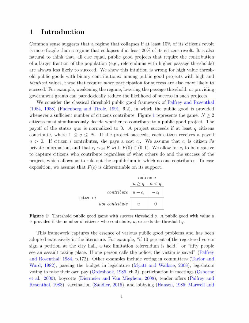
We consider the classical threshold public good framework of Palfrey and Rosenthal
(1984, 1988) (Fudenberg and Tirole, 1991, 6.2), in which the public good is provided
whenever a sufficient number of citizens contribute. Figure 1 represents the game. N ≥ 2
citizens must simultaneously decide whether to contribute to a public good project. The
payoff of the status quo is normalized to 0. A project succeeds if at least q citizens
contribute, where 1 ≤ q ≤ N . If the project succeeds, each citizen receives a payoff
u > 0. If citizen i contributes, she pays a cost ci. We assume that ci is citizen i’s
private information, and that ci ∼iid F with F (0) ∈ (0, 1). We allow for ci to be negative
to capture citizens who contribute regardless of what others do and the success of the
project, which allows us to rule out the equilibrium in which no one contributes. To ease
exposition, we assume that F (c) is differentiable on its support.
citizen i
outcomen ≥ q n < q
contribute u− ci −ci
not contribute u 0
Figure 1: Threshold public good game with success threshold q. A public good with value uis provided if the number of citizens who contribute, n, exceeds the threshold q.
This framework captures the essence of various public good problems and has been
adopted extensively in the literature. For example, “if 10 percent of the registered voters
sign a petition at the city hall, a tax limitation referendum is held,” or “fifty people
see an assault taking place. If one person calls the police, the victim is saved” (Palfrey
and Rosenthal, 1984, p.172). Other examples include voting in committees (Taylor and
Ward, 1982), passing the budget in legislature (Myatt and Wallace, 2008), legislators
voting to raise their own pay (Ordeshook, 1986, ch.3), participation in meetings (Osborne
et al., 2000), boycotts (Diermeier and Van Mieghem, 2008), tender offers (Palfrey and
Rosenthal, 1988), vaccination (Sandler, 2015), and lobbying (Hansen, 1985; Marwell and
1
Oliver, 1991), as well as the ratification of international treaties (Saijo and Yamato, 1999),
and joining an alliance in a world war (Goeree and Holt, 2005). The large experimental
literature that uses this framework includes Dawes et al. (1986), Offerman et al. (1996),
Cadsby and Maynes (1999), Spiller and Bolle (2017), and Palfrey et al. (2017).
Our main result compares analytically the likelihood of public good provision for dif-
ferent success thresholds when the value of public good u is sufficiently small or sufficiently
large (Theorem 1). We prove that when the value of public good u is small, the likelihood
that the project succeeds is decreasing in the threshold q. This is consistent with the
common sense that easier projects are more likely to succeed. In sharp contrast, we prove
that when the value of public good u is sufficiently large, the likelihood that the project
succeeds is increasing in the threshold q for cost distributions with bounded support,
or with asymptotically increasing hazard rate.1 We provide simulations to glean insight
about how the likelihood of success varies with the success threshold for intermediate
public good values.
The direct effect of raising the success threshold q reduces the likelihood of success:
for the same citizens’ behavior, it is less likely that at least q+ 1 of them contribute than
that at least q of them contribute. But there is also an indirect effect. A higher success
threshold changes the probability that a citizen is pivotal, and hence her incentives to
contribute. When the public good value u is large, a higher success threshold raises the
probability of pivotality and hence contribution incentives. We characterize when this
indirect effect dominates.
To see that the indirect effect can dominate, consider the special case with unanimity
and bounded support for contribution costs: N = 2, ci ∼iid U [−1, 1], and u = 1. For
q = 2, there is a unique symmetric equilibrium in which both citizens contribute and
the likelihood of success is 1. When the success threshold falls from q = 2 to q = 1 and
citizens do not adjust their behavior, the probability of success remains 1. So the direct
effect is null. But the probability of being pivotal decreases, so each citizen contributes
less, thereby reducing the likelihood of success.
One may conjecture that the logic of unanimity is the key driver of the result. If it
were so, moving from q = N −1 to unanimity would always raise the likelihood of success
for sufficiently high public good values. This conjecture is wrong. The simplicity of the
example stems from the bounded support of contribution costs, not unanimity. Focusing
on distributions with power-law right tails (Pr(ci > x) = x−α, with α > 0, e.g., Pareto
distribution), we prove that, when public good value is sufficiently large, the likelihood of
success is increasing in q if and only if α > 1 (Proposition 1). When α ≤ 1, the likelihood
of success is decreasing in q, no matter how high the public good value is even when we
raise q to unanimity. As we will show, the key, instead, is the rate at which 1− F falls.
Our results generate counter-intuitive predictions in many settings. When legislators
1That is, when 1− F (c) is log-concave for sufficiently large c. If f(c) is log-concave, so is 1− F (c).
2

are voting to grant themselves a pay raise (u), higher supermajority requirements (higher
q) may lead to higher probability of a raise, especially when the raise is large relative to the
public backlash from voting yes on this unpopular issue (c).2 Strengthening a moderately
unpopular regime (raising q when u is moderate) makes it more likely to survive, while
strengthening a more unpopular regime (raising q when u is large) leads to its collapse.
Our results also speak to the effect of government grants on the likelihood of threshold
public good provision. Government grants in our setting correspond to reducing the suc-
cess threshold q. Our results suggest that government grants may decrease the likelihood
that a public good project succeeds. This result contrasts with the effect of government
grants in the literature on public goods and charitable donations, in which the crowding
out effect of government grant never more than eliminates the value of the grant (Roberts,
1984; Bergstrom et al., 1986; Andreoni and Payne, 2003). In these models, for a fixed level
of public good, a citizen’s incentive to contribute weakly increases with the fraction of
the good financed by the government. In contrast, in our model, the effect of government
contributions on the relationship between the probability of success and citizen incentives
(captured by the probability of pivotality) is more complex.3
Our focus is on how variations in the success threshold q affect the likelihood a public
good project succeeds for a given group size N . In Section 3, we generalize our main
result, e.g., showing how the likelihood of success depends on N − q and the distribution
of contribution costs when the public good value u is sufficiently large (Theorem 2). This
result contributes to the long-standing question of the relationship between public good
provision and group size, dating back to Olson (1965).
Our paper is also related to the literature on the underdog effect in elections, in which
the turnout rate of the majority is lower than the minority due to higher free riding
incentives (Levine and Palfrey, 2007; Krasa and Polborn, 2009; Taylor and Yildirim,
2010; Myatt, 2015). In these models, the threshold q is endogenously determined by voter
turnout. They show that raising a candidate’s popularity can be completely offset by free
riding, but free riding does not dominate the direct effect of higher popularity, and the
2Spenkuch et al. (2018) and Shakiba (2019) provide evidence that U.S. Senators routinely behave asif it is costly for them to vote for their preferred outcome, and that Senators vote strategically, based onpivotality considerations.
3These differences stem from different modeling choices. The cited models consider continuous con-tribution and public good levels, but abstract from strategic uncertainties that arise from asymmetricinformation. We follow the literature with binary contribution and public good levels, but allow forasymmetric information. Investigating the combination of these features is left for future work. However,two points are noteworthy. (1) The intuition for our results suggests that they qualitatively extend whenthe feasible contribution set is sufficiently coarse. In many applications, there are effectively few possiblecontribution levels as social norms or other costs restrict contributions to a few salient levels, or the natureof contribution is discrete (e.g., volunteering time and skills for Habitat for Humanity). At the same time,asymmetric information seems to play an important role in those applications. (2) Similar results arisein the cited models if the warm glow payoff that citizens receive from their contributions is increasing inthe contributions of other citizens, but not the government’s—so that government contribution can lowerthe marginal benefit of contributions for each level of public good.
3
more popular candidate is always weakly more likely to win.4
2 Analysis
The strategy of citizen i is a mapping from her private information ci to a decision whether
to contribute. Fix a strategy profile of citizens other than i, σ−i, and let Pr (piv|σ−i) be
the probability that i is pivotal given σ−i. Then citizen i with cost ci contributes to the
project if ci < Pr (piv|σ−i)u and does not contribute if ci > Pr (piv|σ−i)u. Thus, the best
response of player i is a threshold strategy. We focus on symmetric equilibria.5 Since
F (0) ∈ (0, 1), equilibrium threshold c∗q(u) is characterized by the indifference condition6
c∗q(u)
u=
(N − 1
q − 1
)(F(c∗q(u)
))q−1 (1− F (c∗q(u))
)N−q ≡ Pr(piv|q, c∗q(u)
). (1)
Let Sq(c∗q(u)) be the probability of success corresponding to the equilibrium threshold
c∗q(u). Then,
Sq(c∗q(u)) =
N∑k=q
(N
k
)(F(c∗q(u)
))k (1− F
(c∗q(u)
))N−k(2)
= 1−q−1∑k=0
(N
k
)(F(c∗q(u)
))k (1− F
(c∗q(u)
))N−k. (3)
Our goal is to characterize how changes in q affect the equilibrium probability of success
Sq(c∗q(u)). For a general public good value, this analysis is intractable. We prove results
for the polar opposite cases where the public good value is sufficiently small or sufficiently
large.
Theorem 1. If the support of costs is bounded from above, or if 1− F (x) is log-concave
for sufficiently large x, then the likelihood of success is increasing in the success threshold
when the public good value is sufficiently large: Sq+1(c∗q+1(u)) > Sq(c∗q(u)) for sufficiently
large u. In contrast, the likelihood of success is always decreasing in the success threshold
when the public good value is sufficiently small: Sq+1(c∗q+1(u)) < Sq(c∗q(u)) for sufficiently
small u.
The result is driven by the interplay of two effects. When the threshold q required
for success increases to q + 1, the direct effect decreases the probability of success: fixing
4In Myatt (2015), a candidate who is more popular but less popular than expected will lose, butraising candidate’s realized popularity improves her chances.
5For a defense of symmetric equilibria see Palfrey and Rosenthal (1984) and Dixit and Olson (2000).6When the distribution of costs has bounded support, the threshold that satisfies the indifference
condition may be above the upper bound of the support, in which case F(c∗q(u)
)= 1.
4
citizen behavior, it is less likely that at least q + 1 of them contribute than that at least
q of them contribute. However, there is an indirect effect. As q increases, the probability
that citizen i is pivotal also changes, which affects her behavior.
When the value of public good u is large, each citizen contributes with large probability,
so it is more likely that exactly q citizens other than i contribute than that exactly q− 1
citizens other than i contribute. Thus, as q increases to q + 1, citizen i becomes more
likely to be pivotal, and hence she increases her contribution threshold. So the indirect
effect counters the direct effect. For the indirect effect to dominate, it must be that as the
equilibrium threshold increases, the expected number of new participants (those whose
participation costs cis are just above the old equilibrium threshold c∗q) is sufficiently large.
When F (c) increases more quickly, it means there are more such citizens; and a bounded
support or log-concavity of 1− F (c) means that F (c) increases sufficiently fast.
In contrast, when the value of public good u is sufficiently small, even an increase in
the probability of pivotality has a negligible effect on citizens’ incentives to contribute.
Therefore, the direct effect always dominates the indirect effect, so the likelihood of success
decreases.7
Theorem 1 does not address whether our result for large public good values extends
to distributions with thicker right tails for which 1 − F (x) is not log-concave for large
x. Proposition 1 provides the analysis for the class of distributions with power-law right
tails (e.g., Pareto distribution).
Proposition 1. Suppose 1 − F (x) = β/xα, α, β > 0, for sufficiently large x. When the
public good value is sufficiently large, the likelihood of success is increasing in the success
threshold, Sq+1(c∗q+1(u)) > Sq(c∗q(u)), if and only if α > 1.
Three points are worth highlighting. First, combining Theorem 1 and Proposition 1
suggests that 1/x is close to the boundary tail distribution that separates cost distributions
for which the strategic effect dominates (thinner than Cauchy) from those for which
the direct effect dominates (thicker than Cauchy)—recall that for the standard Cauchy
distribution, Pr(ci > x) ≈ 1/πx for large x.
Second, based on our simple example in the Introduction, one may have thought that
unanimity is the key for a higher success threshold to increase the chances of success
when u is sufficiently large. However, unanimity is neither necessary nor sufficient for
this result. It is not sufficient because raising the success threshold from q = N − 1 to
q + 1 = N reduces the likelihood of success when 1 − F (x) = x−α for α ≤ 1, no matter
how large u is. It is not necessary because raising the success threshold at any level (e.g.,
7When u is small, each citizen contributes with probability close to F (0). When F (0) is small, theprobability of being pivotal decreases with q: if each citizen contributes with low probability, it is lesslikely that exactly q citizens other than i contribute than that exactly q−1 citizens other than i contribute.In this case, the indirect effect strengthens the direct effect.
5
from q = N − 3 to q + 1 = N − 2) increases the likelihood of success when 1− F (x) goes
to 0 faster and u is sufficiently large.8
Third, a higher success threshold increases the chances of success only if it raises the
contribution threshold: Sq+1(c∗q+1) > Sq(c∗q) requires c∗q+1 > c∗q. This may lead one to
conjecture that a very large c∗q+1/c∗q is sufficient for Sq+1(c∗q+1) > Sq(c
∗q). This conjecture
is incorrect. To see this, suppose 1 − F (x) = x−α with α > 0 for large x, and compare
c∗N(u) and c∗1(u) when u is very large. The indifference conditions imply
limu→∞
c∗N(u)
u= 1 and lim
u→∞
c∗1(u)
u1
1+α(N−1)
= 1.
Thus, c∗N(u)/c∗1(u) can be made arbitrary large by choosing a sufficiently large u. However,
Proposition 1 shows that, no matter how large u becomes, SN(c∗N(u)) < S1(c∗1(u)) for
α ∈ (0, 1]. In fact, when q ∈ {1, · · · , N − 2}, for Sq+1(c∗q+1(u)) > Sq(c∗q(u)) to hold for
sufficiently large u, c∗q+1/c∗q must not be too large.9 To see this, consider equations (1)
and (3) and suppose u is very large. A citizen almost always contributes, so that the
dominant term in these equations is 1− F (c∗q(u)) with the lowest power
Pr(piv|q, c∗q) ≈(N − 1
q − 1
)(1− F (c∗q)
)N−qand Sq(c
∗q) ≈ 1−
(N
q − 1
)(1− F
(c∗q))N−q+1
.
For Sq+1(c∗q+1) > Sq(c∗q), we want
(1− F
(c∗q+1
))N−qto be as small as possible. But
this does not mean that we want c∗q+1 to be as large as possible, because c∗q+1 is an
equilibrium object and is linked to(1− F
(c∗q+1
))N−qthrough the likelihood of pivotality:
in equilibrium, if c∗q+1 is higher, then so is 1 − F (c∗q+1). Rather, as Theorem 1 and
Proposition 1 show, the key is how fast 1 − F falls. When raising q to q + 1, if the
equilibrium contribution threshold did not change, we would have(N − 1
q
)(1− F (c∗q)
)N−(q+1)>
(N − 1
q − 1
)(1− F (c∗q)
)N−q ≈ c∗qu.
But now the equilibrium contribution threshold increases to c∗q+1 to restore indifference:(N − 1
q
)(1− F (c∗q+1)
)N−(q+1) ≈c∗q+1
u.
It follows that the faster 1 − F (·) drops around c∗q, the lower will be 1 − F (c∗q+1), and
hence the higher will be Sq+1(c∗q+1).
Our analytical results focus on the asymptotic cases when the public good value is very
8Moreover, note that for all q ∈ {1, · · · , N − 1}, unlike for unanimity, each player is unlikely to bepivotal even when u is very large, while each player contributes with probability close to 1.
9See part (iii) of Lemma 1 in the Appendix.
6
small or very large. How does the likelihood of success vary with the success threshold for
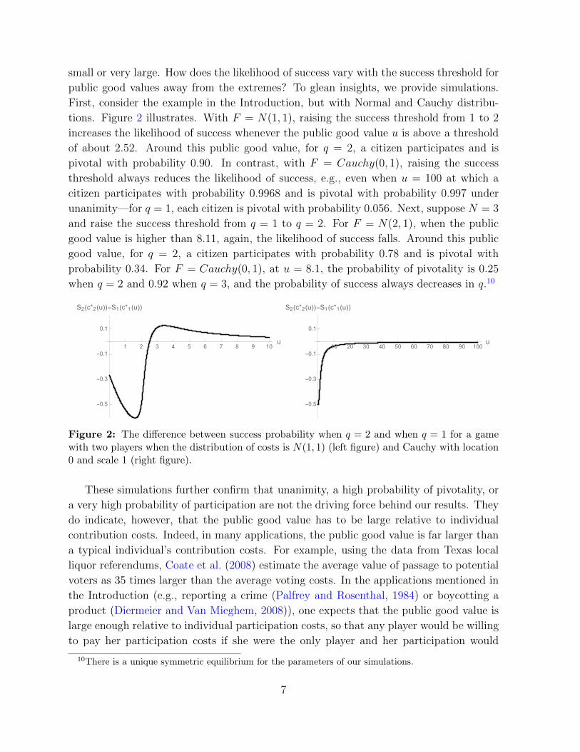
public good values away from the extremes? To glean insights, we provide simulations.
First, consider the example in the Introduction, but with Normal and Cauchy distribu-
tions. Figure 2 illustrates. With F = N(1, 1), raising the success threshold from 1 to 2
increases the likelihood of success whenever the public good value u is above a threshold
of about 2.52. Around this public good value, for q = 2, a citizen participates and is
pivotal with probability 0.90. In contrast, with F = Cauchy(0, 1), raising the success
threshold always reduces the likelihood of success, e.g., even when u = 100 at which a
citizen participates with probability 0.9968 and is pivotal with probability 0.997 under
unanimity—for q = 1, each citizen is pivotal with probability 0.056. Next, suppose N = 3
and raise the success threshold from q = 1 to q = 2. For F = N(2, 1), when the public
good value is higher than 8.11, again, the likelihood of success falls. Around this public
good value, for q = 2, a citizen participates with probability 0.78 and is pivotal with
probability 0.34. For F = Cauchy(0, 1), at u = 8.1, the probability of pivotality is 0.25
when q = 2 and 0.92 when q = 3, and the probability of success always decreases in q.10
1 2 3 4 5 6 7 8 9 10u
-0.5
-0.3
-0.1
0.1
S2(c*2(u))-S1(c
*1(u))
10 20 30 40 50 60 70 80 90 100u
-0.5
-0.3
-0.1
0.1
S2(c*2(u))-S1(c
*1(u))
Figure 2: The difference between success probability when q = 2 and when q = 1 for a gamewith two players when the distribution of costs is N(1, 1) (left figure) and Cauchy with location0 and scale 1 (right figure).
These simulations further confirm that unanimity, a high probability of pivotality, or
a very high probability of participation are not the driving force behind our results. They
do indicate, however, that the public good value has to be large relative to individual
contribution costs. Indeed, in many applications, the public good value is far larger than
a typical individual’s contribution costs. For example, using the data from Texas local
liquor referendums, Coate et al. (2008) estimate the average value of passage to potential
voters as 35 times larger than the average voting costs. In the applications mentioned in
the Introduction (e.g., reporting a crime (Palfrey and Rosenthal, 1984) or boycotting a
product (Diermeier and Van Mieghem, 2008)), one expects that the public good value is
large enough relative to individual participation costs, so that any player would be willing
to pay her participation costs if she were the only player and her participation would
10There is a unique symmetric equilibrium for the parameters of our simulations.
7
deliver the good.
3 Generalized Theorem
Our intuition suggests a close link between the effect of raising the success threshold q
and reducing the group size N . We now extend Theorem 1, showing how the likelihood of
success depends on N − q. We state the generalized theorem below, and provide its proof
and the analogous generalization of Proposition 1 in an Online Appendix. Let c∗q,N(u) be
the symmetric equilibrium threshold in the game with success threshold q and N players.
Theorem 2. Take q, N , q′ and N ′ such that q ≤ N and q′ ≤ N ′.
1. If q ≤ q′ and N − q ≥ N ′ − q′, with at least one inequality strict, then Sq,N(c∗q,N(u)) >
Sq′,N ′(c∗q′,N ′(u)) for sufficiently small u.
2. Suppose the support of costs is bounded from above, or 1 − F (x) is log-concave for
sufficiently large x. If N − q < N ′ − q′, then Sq,N(c∗q,N(u)) > Sq′,N ′(c∗q′,N ′(u)) for
sufficiently large u.
Theorem 2 sheds light on the long-standing question of the relationship between group
size and public good provision. Olson (1965) argued that larger groups are less likely to
provide public goods because they have a more severe free riding problem. However,
Chamberlin (1974) (and many since) showed that Olson’s conjecture does not hold in
standard public good models like Bergstrom et al. (1986).11 The direct effect of raising
group size dominates the strategic, free riding effect, so that larger groups provide more
public goods. In symmetric mixed strategy equilibria of the complete information thresh-
old public good game with q = 1 (analyzed in Palfrey and Rosenthal (1984)), Diekmann
(1985) showed that the probability of success is decreasing in group size N . We show
this result is not robust to the strategic uncertainty introduced by private participation
costs.12 When the public good value is small, the likelihood of public good provision is
increasing in N . In contrast, for sufficiently valuable public goods, the strategic effect
dominates and Olson’s conjecture holds for any success threshold q ≤ N if either the
distribution of contribution costs are bounded from above or have log-concave right tails.
Our generalization of Proposition 1 (in the Online Appendix) shows that when the right
11In Esteban and Ray (2001), multiple groups compete for a prize. When the prize is a purely publicgood, the probability of success is increasing in group size.
12In particular, consider ci = c+ σεi. For any σ, Diekmann’s result is overturned for sufficiently smallu if F (ci) satisfies our conditions, and for sufficiently large u if the distribution of εi has fat tails. Ina dynamic extension of Palfrey and Rosenthal (1984, 1988), Yildirim (2006) finds that in later periodswhen dynamic incentives are absent, participation is decreasing in group size when participation costshave bounded support.
8
tail distribution of participation costs is fatter than Cauchy, Olson’s conjecture is reversed
even for very high value public goods.13
4 Conclusion
Public good projects that require fewer contributors to succeed may seem to have a higher
chance of success. That fewer contributors are needed for success may increase free riding
incentives, but common sense suggests that this strategic effect should not offset the direct
effect. We show that in a standard threshold public good game with binary contributions,
this intuition fails under quite standard conditions.
Several directions for future research stand out. (1) We focused on threshold public
good with binary contributions. The analogous analysis with multiple contribution levels
is left to future research. (2) We analyzed the standard case in which costs are uncorre-
lated. Shadmehr (2019) provides a partial characterization of the same game in the limit
when the number of citizens is large and costs have common and idiosyncratic compo-
nents. With a numerical example, he shows that with Normal prior about the common
cost component, the likelihood of success can be increasing in the success threshold. Ana-
lyzing the problem for intermediate correlation levels remains to be done. (3) The simple
setting makes testing predictions in lab experiments feasible and especially valuable given
the counter-intuitive nature of the results.
13Deserranno et al. (2020) look at a random entry of NGOs into areas of Uganda that already havegovernment-provided healthcare workers. The entry by NGOs reduces the probability of receiving healthcare from any healthcare worker (as measured by whether a household received medical care in the pastyear) by twelve percentage points. This finding is consistent with part 2 of Theorem 2 in that increasingthe number of potential healthcare providers leads to a lower probability of healthcare provision.
9
Appendix: Proofs
To ease the exposition, we drop superscript ∗ in c∗q(u), and write cq(u) or cq for equilibrium
thresholds, recognizing that cq depends on model parameters, including u. We also use
Sq(u) for Sq(c∗q(u)).
We begin with a preliminary lemma that will be used in the proof of Theorem 1. Part
(iii) of this lemma bounds cq+1
cqas u → ∞. As discussed in the main text, ensuring that
cq+1
cqis not too large is crucial for the argument.
Lemma 1. (i) limu→∞cN (u)u
= 1. Moreover, if the support of costs is bounded from above,
or if 1−F (x) is log-concave for sufficiently large x, then (ii) for all α > 0, limu→∞cq(u)
uα= 0
if q < N , and (iii) limu→∞cq+1(u)
cq(u)<∞ if q < N − 1.
Proof of Lemma 1. Part (i) directly follows from (1).
To prove parts (ii) and (iii), suppose first the support of costs is bounded from above.
Then for q < N , cq(u) is strictly smaller than the upper bound of the cost distribution,
so it is bounded from above (which proves part (ii)), and bounded away from 0 (which
proves part (iii)).
Next, suppose the support of costs does not have an upper bound, but 1 − F (x) is
log-concave for sufficiently large x.
Part (ii). Differentiating (1) with respect to u yields
dcq(u)
du=
(N−1q−1
)(F (cq))
q−1 (1− F (cq))N−q
1− u(N−1q−1
)(F (cq))
q−2 (1− F (cq))N−q−1 ((q − 1) (1− F (cq))− (N − q)F (cq)) f (cq)
.
(4)
From (1), the numerator is equal to cqu
, and also(N − 1
q − 1
)(F (cq))
q−2 (1− F (cq))N−q−1 =
cq(u)
u
1
F (cq) (1− F (cq)). (5)
Substituting cqu
and (5) into (4) yields:
dcq(u)
du=
cqu
1− u cqu
1F (cq)(1−F (cq))
((q − 1) (1− F (cq))− (N − q)F (cq)) f (cq)
=1
u
1
1cq−(
(q − 1)1−F (cq)
F (cq)− (N − q)
)f(cq)
1−F (cq)
. (6)
From (1), limu→∞ cq(u) =∞, and hence limu→∞ F (cq(u)) = 1. Using L’Hopital’s rule, we
10

have
limu→∞
cq(u)
uα= lim
u→∞
dcq(u)
du
αuα−1
= limu→∞
1
u
1
1cq−(
(q − 1)1−F (cq)
F (cq)− (N − q)
)f(cq)
1−F (cq)
1
αuα−1(from (6))
= limu→∞
1
α
1
1−(
(q − 1)1−F (cq)
F (cq)− (N − q)
)f(cq)
1−F (cq)cq
cquα.
Since 1− F is log-concave, limu→∞f(cq(u))
1−F (cq(u))> 0, and the second line above implies that
limu→∞cq(u)
uα<∞, so we can move limu→∞
cq(u)
uαto one side, obtaining
limu→∞
cq(u)
uα
1− 1
α
1
1−(
(q − 1)1−F (cq)
F (cq)− (N − q)
)f(cq)
1−F (cq)cq
= 0.
Because limu→∞f(cq)
1−F (cq)> 0, the limit of the term in the parenthesis is not 0 for any α,
and hence limu→∞cq(u)
uα= 0.
Part (iii). By contradiction, suppose that limu→∞cq+1(u)
cq(u)=∞. Then, cq+1(u) > cq(u)
for sufficiently large u. Because 1− F is log-concave, f1−F is increasing, and hence
limu→∞
f(cq(u))
1−F (cq(u))
f(cq+1(u))
1−F (cq+1(u))
<∞. (7)
Moreover, using L’Hopital’s rule, we obtain
limu→∞
cq+1(u)
cq(u)= lim
u→∞
dcq+1(u)
dudcq(u)
du
= limu→∞
1cq−(
(q − 1)1−F (cq)
F (cq)− (N − q)
)f(cq)
1−F (cq)
1cq+1−(q 1−F (cq+1)
F (cq+1)− (N − q − 1)
)f(cq+1)
1−F (cq+1)
(from (6))
= limu→∞
N − qN − q − 1
f(cq(u))
1−F (cq(u))
f(cq+1(u))
1−F (cq+1(u))
<∞ (from (7)),
which is a contradiction.
We now provide the proof of Theorem 1.
Proof of Theorem 1. First, we prove the second part of the theorem pertaining to low
11

u. From (1), cq(0) = cq+1(0) = 0. Thus, from (2),
Sq+1(0)− Sq(0) =N∑
k=q+1
(N
k
)(F (0))k (1− F (0))N−k −
N∑k=q
(N
k
)(F (0))k (1− F (0))N−k
= −(N
q
)(F (0))q (1− F (0))N−q < 0.
The result follows from the continuity of cq(u) and Sq(u) in u.
Now, we prove the first part of the theorem. The difference between success probability
for q + 1 and q is as follows:
Sq+1(u)− Sq(u) = (1− Sq(u))
(1− 1− Sq+1(u)
1− Sq(u)
).
Thus, it suffices to show
limu→∞
1− Sq+1(u)
1− Sq(u)< 1.
From (3),
1− Sq+1(u)
1− Sq(u)=
∑qk=0
(Nk
)(F (cq+1))k (1− F (cq+1))N−k∑q−1
k=0
(Nk
)(F (cq))
k (1− F (cq))N−k
=
∑qk=0
(Nk
)(F (cq+1))k (1− F (cq+1))q−k∑q−1
k=0
(Nk
)(F (cq))
k (1− F (cq))q−1−k
(1− F (cq+1))N−q
(1− F (cq))N−q+1
(8)
Moreover, since limu→∞ F (cq) = limu→∞ F (cq+1) = 1,
limu→∞
q∑k=0
(N
k
)(F (cq+1))k (1− F (cq+1))q−k =
(N
q
), (9)
limu→∞
q−1∑k=0
(N
k
)(F (cq))
k (1− F (cq))q−1−k =
(N
q − 1
). (10)
Substituting (9) and (10) into (8) yields
limu→∞
1− Sq+1(u)
1− Sq(u)= lim
u→∞
(Nq
)(Nq−1
) (1− F (cq+1))N−q
(1− F (cq))N−q+1
. (11)
12
For the rest of the proof, we consider two cases separately: q < N − 1 and q = N − 1.
The latter case corresponds to moving to unanimity, and part (iii) of Lemma 1 does not
apply for this case. Therefore, it requires a different approach.
q < N− 1. From the indifference condition (1),
(1− F (cq))N−q+1 =
(cqu
1(N−1q−1
)(F (cq))
q−1
)N−q+1N−q
, for q ∈ {1, · · · , N − 1},
(1− F (cq+1))N−q =
(cq+1
u
1(N−1q
)(F (cq+1))q
) N−qN−q−1
, for q ∈ {1, · · · , N − 2}.
Substituting these into (11) yields that, for q ∈ {1, · · · , N − 2},
limu→∞
1− Sq+1(u)
1− Sq(u)= lim
u→∞
N − q + 1
q
(cq+1(u)
u1
(N−1q )(F (cq+1(u)))q
) N−qN−q−1
(cq(u)
u1
(N−1q−1 )(F (cq(u)))q−1
)N−q+1N−q
= limu→∞
N − q + 1
q
(1
(N−1q )(F (cq+1(u)))q
) N−qN−q−1
(1
(N−1q−1 )(F (cq(u)))q−1
)N−q+1N−q
(cq+1(u)
cq(u)
)N−q+1N−q
(cq+1(u)
u
) 1(N−q−1)(N−q)
=N − q + 1
q
(1
(N−1q )
) N−qN−q−1
(1
(N−1q−1 )
)N−q+1N−q
(limu→∞
cq+1(u)
cq(u)
)N−q+1N−q
(limu→∞
cq+1(u)
u
) 1(N−q−1)(N−q)
.
From part (ii) of Lemma 1, limu→∞cq+1(u)
u= 0. From part (iii) of Lemma 1,
limu→∞cq+1(u)
cq(u)<∞. Thus, limu→∞
1−Sq+1(u)
1−Sq(u)= 0, and the result follows.
q = N− 1. From (11), it suffices to show
limu→∞
1− SN(u)
1− SN−1(u)= lim
u→∞
2
N − 1
1− F (cN)
(1− F (cN−1))2< 1. (12)
We show limu→∞1−F (cN )
(1−F (cN−1))2= 0. If the support of costs is bounded from above,
then 1 − F (cN(u)) = 0 for sufficiently large u, while 1 − F (cN−1(u)) > 0 for all u
although it becomes arbitrarily close to 0. Next, consider the case where the support
13
of costs has no upper bound. From parts (i) and (ii) of Lemma 1, it suffices to show:
limu→∞
1− F (u)
(1− F (uα))2= 0, for some α ∈ (0, 1). (13)
Because 1 − F (x) ∈ (0, 1) is decreasing and log-concave, its right-tail is at most
exponential (An, 1998). In particular, for sufficiently large x, 1 − F (x) goes to 0
faster than x−b, for any b > 0.
Pick an α ∈ (0, 1/2). Fix ε > 0. Pick a sufficiently large x, such that for x > x,
1−F (x) goes to 0 faster than x−b, for any b > 0. Pick x1 > x, and find b1 such that
1− F (xα1 ) = (xα1 )−b1 = x−αb11 . Hence, 1− F (x1) < x−b11 , and hence
1− F (x1)
(1− F (xα1 ))2=
1− F (x1)
x−2αb11
<x−b11
x−2αb11
=1
xb1(1−2α)1
.
If 1
xb1(1−2α)1
< ε, then set x = ε− 1
(1−2α)b1 . Otherwise, choose x > x1 large enough, so
that 1xb1(1−2α) < ε. Because 1−F (x) goes to 0 faster that x−b1 , there exists a b2 > b1
such that 1− F (xα) = (xα)−b2 = x−αb2 . Thus,
1− F (x)
(1− F (xα))2=
1− F (x)
x−2αb2<
x−b2
x−2αb2=
1
xb2(1−2α)<
1
xb1(1−2α)< ε.
Now, consider x > x. Find b3, so that 1− F (xα) = x−αb3 . Again, because 1− F (x)
goes to 0 faster than x−b, for all b > 0, b3 > b2, and hence 1−F (x)(1−F (xα))2
< ε. The result
follows.
We have shown that for any given q ∈ {1, · · · , N − 1}, Sq+1(u) > Sq(u) for sufficiently
large u. Because there is a finite number of q’s, Sq(u) increases in q for sufficiently large
u.
Proof of Proposition 1. Substituting 1− F (x) = βxα
in (11) yields:
limu→∞
1− Sq+1(u)
1− Sq(u)= lim
u→∞
N − q + 1
βq
((cq(u))N−q+1
(cq+1(u))N−q
)α
. (14)
From indifference condition (1),
cq(u) =
(N − 1
q − 1
)(1− β
(cq(u))α
)q−1(β
(cq(u))α
)N−qu.
14
Thus,
(cq(u))N−q+1 =
((N − 1
q − 1
)βN−q
(1− β
(cq(u))α
)q−1
u
) N−q+1α(N−q)+1
.
Substituting this in (14) yields:
limu→∞
1− Sq+1(u)
1− Sq(u)= lim
u→∞
N − q + 1
βq
((
N−1q−1
)βN−q
(1− β
(cq(u))α
)q−1
u
) N−q+1α(N−q)+1
((N−1q
)βN−q−1
(1− β
(cq+1(u))α
)qu) N−qα(N−q−1)+1
α
= limu→∞
N − q + 1
βq
((
N−1q−1
)βN−qu
) N−q+1α(N−q)+1
((N−1q
)βN−q−1u
) N−qα(N−q−1)+1
α
= limu→∞
N − q + 1
βq
((
N−1q−1
)βN−q
) N−q+1α(N−q)+1
((N−1q
)βN−q−1
) N−qα(N−q−1)+1
α
u( N−q+1α(N−q)+1
− N−qα(N−q−1)+1)α.
Write the power of u as α(α(N−q)+1)(α(N−q−1)+1)
(1−α), and recognize that α(α(N−q)+1)(α(N−q−1)+1)
>
0. Thus,
limu→∞
1− Sq+1(u)
1− Sq(u)=
{0 ;α > 1
∞ ;α < 1, and hence lim
u→∞
(1− 1− Sq+1(u)
1− Sq(u)
)=
{> 0 ;α > 1
< 0 ;α < 1.
When α = 1,
limu→∞
1− Sq+1(u)
1− Sq(u)=N − q + 1
βq
(N−1q−1
)βN−q(
N−1q
)βN−q−1
=N − q + 1
N − q.
Thus, for α = 1, limu→∞
(1− 1−Sq+1(u)
1−Sq(u)
)= − 1
N−q < 0.
References
An, Mark Yuying. 1998. “Logconcavity versus Logconvexity: A Complete Characteri-
zation.” Journal of Economic Theory, 80(2): 350–369.
Andreoni, James, and A. Abigail Payne. 2003. “Do Government Grants to Private
15
Charities Crowd Out Giving or Fund-raising?” American Economic Review, 93(3):
792–812.
Bergstrom, Ted, Larry Blume, and Hal Varian. 1986. “On the Private Provision
of Public Goods.” Journal of Public Economics, 29 25–49.
Cadsby, Charles Bram, and Elizabeth Maynes. 1999. “Voluntary Provision of
Threshold Public Goods with Continuous Contributions: Experimental Evidence.”
Journal of Public Economics, 71(1): 53–73.
Chamberlin, John R. 1974. “Provision of Collective Goods as a Function of Group
Size.” American Political Science Review, 68 707–716.
Coate, Stephen, Michael Conlin, and Andrea Moro. 2008. “The performance of
pivotal-voter models in small-scale elections: Evidence from Texas liquor referenda.”
Journal of Public Economics, 92 582–596.
Dawes, Robyn M., John M. Orbell, Randy T. Simmons, and Alphons J.C.
Van De Kragt. 1986. “Organizing Groups for Collective Action.” American Political
Science Review 1171–1185.
Deserranno, Erica, Aisha Nansamba, and Nancy Qian. 2020. “Aid Crowd-Out:
The Effect of NGOs on Government-Provided Public Services.” URL: https://drive.
google.com/file/d/129-OnnpwhaTgDdaC1VNJC1EbNscNan4-/view.
Diekmann, Andreas. 1985. “Volunteer’s Dilemma.” Journal of Conflict Resolution, 29
605–610.
Diermeier, Daniel, and Jan A. Van Mieghem. 2008. “Voting with your
Pocketbook—A Stochastic Model of Consumer Boycotts.” Mathematical and Computer
Modelling, 48 1497–1509.
Dixit, Avinash, and Mancur Olson. 2000. “Does Voluntary Participation Undermine
the Coase Theorem?” Journal of Public Economics, 76(3): 309–335.
Esteban, Joan, and Debraj Ray. 2001. “Collective Action and the Group Size Para-
dox.” American Political Science Review 663–672.
Fudenberg, Drew, and Jean Tirole. 1991. Game Theory. Cambridge: MIT Press.
Goeree, Jacob K., and Charles A. Holt. 2005. “An Explanation of Anomalous Be-
havior in Models of Political Participation.” American Political Science Review, 99(2):
201–213.
16

Hansen, John Mark. 1985. “The Political Economy of Group Membership.” The Amer-
ican Political Science Review 79–96.
Krasa, Stefan, and Mattias K. Polborn. 2009. “Is Mandatory Voting Better than
Voluntary Voting?” Games and Economic Behavior, 66(1): 275–291.
Levine, David K., and Thomas R. Palfrey. 2007. “The Paradox of Voter Participa-
tion? A Laboratory Study.” American Political Science Review, 101(1): 143–158.
Marwell, Gerald, and Pamela E. Oliver. 1991. “A Theory of the Critical Mass.” In
Disziplin und Kreativitat.: Springer, 49–62.
Myatt, David P. 2015. “A Theory of Voter Turnout.” URL: http://dpmyatt.org/
uploads/turnout-2015.pdf.
Myatt, David P., and Chris Wallace. 2008. “When Does One Bad Apple Spoil the
Barrel? An Evolutionary Analysis of Collective Action.” The Review of Economic
Studies, 75(2): 499–527.
Offerman, Theo, Joep Sonnemans, and Arthur Schram. 1996. “Value Orientations,
Expectations and Voluntary Contributions in Public Goods.” The Economic Journal,
106(437): 817–845.
Olson, Mancur. 1965. The Logic of Collective Action: Public Goods and the Theory of
Groups.: Harvard University Press.
Ordeshook, Peter C. 1986. Game Theory and Political Theory: An Introduction.: Cam-
bridge University Press.
Osborne, Martin J., Jeffrey S. Rosenthal, and Matthew A. Turner. 2000. “Meet-
ings with Costly Participation.” American Economic Review, 90(4): 927–943.
Palfrey, Thomas, and Howard Rosenthal. 1984. “Participation and the Provision
of Discrete Public Goods: A Strategic Analysis.” Journal of Public Economics, 24(2):
171–193.
Palfrey, Thomas, and Howard Rosenthal. 1988. “Private Incentives in Social Dilem-
mas.” Journal of Public Economics, 35(2): 309–332.
Palfrey, Thomas, Howard Rosenthal, and Nilanjan Roy. 2017. “How Cheap Talk
Enhances Efficiency in Threshold Public Goods Games.” Games and Economic Behav-
ior, 101 234–259.
Roberts, Russell D. 1984. “A Positive Model of Private Charity and Public Transfers.”
Journal of Political Economy, 92(1): 136–148.
17

Saijo, Tatsuyoshi, and Takehiko Yamato. 1999. “A Voluntary Participation Game
with a Non-excludable Public Good.” Journal of Economic Theory, 84(2): 227–242.
Sandler, Todd. 2015. “Collective Action: Fifty Years Later.” Public Choice, 164(1):
195–216.
Shadmehr, Mehdi. 2019. “Protest Puzzles: Tullock’s Paradox, Hong Kong Experiment,
and the Strength of Weak States.” forthcoming in Quarterly Journal of Political Science.
Shakiba, Mehdi. 2019. “Do Senators Take Strategic Advantage of their Last Names?”,
URL: https://drive.google.com/file/d/1ByKd57urIxJmOuaaT-7YBbMxwZv3DGsU/
view.
Spenkuch, Jorg, Pablo Montagnes, and Daniel Magleby. 2018. “Backward Induc-
tion in the Wild? Evidence from Sequential Voting in the U.S. Senate.” The American
Economic Review, 108(7): 1971–2013.
Spiller, Jorg, and Friedel Bolle. 2017. “Experimental Investigations of Binary Thresh-
old Public Good Games.” URL: https://ideas.repec.org/p/zbw/euvwdp/393.html.
Taylor, Curtis R., and Huseyin Yildirim. 2010. “Public Information and Electoral
Bias.” Games and Economic Behavior, 68(1): 353–375.
Taylor, Michael, and Hugh Ward. 1982. “Chickens, Whales, and Lumpy Goods:
Alternative Models of Public-Goods Provision.” Political Studies, 30(3): 350–370.
Yildirim, Huseyin. 2006. “Getting the Ball Rolling: Voluntary Contributions to a
Large-Scale Public Project.” Journal of Public Economic Theory, 8(4): 503–528.
18


