
Soil Sensor
Stevens® Water Monitoring Systems, Inc. Monitoring Earth’s Water Resources Since 1911
®
Users Manual January 2018
Rev. VI
Firmware version 2.9
2
Safety and Equipment Protection
WARNING!
ELECTRICAL POWER CAN RESULT IN DEATH, PERSONAL INJURY OR CAN CAUSE DAMAGE TO EQUIPMENT. If the instrument is driven by an external
power source, disconnect the instrument from that power source before attempting any repairs. WARNING! BATTERIES ARE DANGEROUS. IF HANDLED IMPROPERLY, THEY CAN RESULT IN DEATH, PERSONAL INJURY OR CAN CAUSE DAMAGE TO EQUIPMENT. Batteries can be hazardous when misused, mishandled, or disposed of improperly. Batteries contain potential energy, even when partially discharged.
WARNING! ELECTRICAL SHOCK CAN RESULT IN DEATH OR PERSONAL INJURY. Use extreme caution when handling cables, connectors, or terminals; they may yield
hazardous currents if inadvertently brought into contact with conductive materials, including water and the human body.
CAUTION! Be aware of protective measures against environmentally caused electric current surges and follow the previous warnings and cautions, the following safety activities should be carefully observed.
Children and Adolescents. NEVER give batteries to young people who may not be aware of the hazards associated with batteries and their improper use or disposal.
Jewelry, Watches, Metal Tags To avoid severe burns, NEVER wear rings, necklaces, metal watch bands, bracelets, or metal identification tags near exposed battery terminals.
Heat, Fire NEVER dispose of batteries in fire or locate them in excessively heated spaces. Observe the temperature limit listed in the instrument specifications.
Charging NEVER charge "dry" cells or lithium batteries that are not designed to be charged.
NEVER charge rechargeable batteries at currents higher than recommended ratings.
NEVER recharge a frozen battery. Thaw it completely at room temperature before connecting charger.
Unvented Container
NEVER store or charge batteries in a gas-tight container. Doing so may lead to pressure buildup and explosive concentrations of hydrogen.
Short Circuits
NEVER short circuit batteries. High current flow may cause internal battery heating and/or explosion.
Damaged Batteries
Personal injury may result from contact with hazardous materials from a damaged or open battery. NEVER attempt to open a battery enclosure. Wear appropriate protective clothing, and handle damaged batteries carefully.
Disposal ALWAYS dispose of batteries in a responsible manner. Observe all applicable federal, state, and local regulations for disposal of the specific type of battery involved.
NOTICE Stevens makes no claims as to the immunity of its equipment against lightning strikes, either direct or nearby.
The following statement is required by the Federal Communications Commission:
WARNING
This equipment generates, uses, and can radiate radio frequency energy and, if not installed in accordance with the instructions manual, may cause interference to radio communications. It has been tested and found to comply with the limits for a Class A computing device pursuant to Subpart J of Part 15 of FCC Rules, which are designed
to provide reasonable protection against such interference when operated in a commercial environment. Operation of this equipment in a residential area is likely to cause
interference in which case the user at their own expense will be required to take whatever measures may be required to correct the interference.
USER INFORMATION
Stevens makes no warranty as to the information furnished in these instructions and the reader assumes all risk in the use thereof. No liability is assumed for damages resulting from the use of these instructions. We reserve the right to make changes to products and/or publications without prior notice.

3
Preface This manual is a comprehensive guide to the Stevens HydraProbe Soil Sensor. Contained within this manual is
a theoretical discussion of soil physics that explains the theory behind how electromagnetic soil sensors work as
well as a discussion about vadose zone hydrology. References to peer reviewed scientific publications are
provided to give the user further background on these topics. Because soil moisture monitoring is becoming
increasingly important to researchers across a broad number of fields including hydrology, agronomy, soil
physics, and geotechnical engineering, we feel it is necessary to include advanced theoretical discussions with
references to help the scientists and engineers understand the measurement technology in a manner that is
unbiased and referenced.
Easy to Use
Despite this sophistication, Stevens HydraProbe Soil Sensor is also very easy to use. The user may skip to
chapter 3 to learn about the installation and reference Appendix A for SDI-12 probes and Appendix B for
RS485 Probes for wiring and communication. Calibration is not necessary for most soils and the default settings
will accommodate most users and applications.

4
Comprehensive Stevens HydraProbe User's Manual
Table of Contents
1 Introduction 6 1.1 Applications ................................................................................................................................. 7 1.2 Calibrations .................................................................................................................................. 7 1.3 Dielectric Permittivity ................................................................................................................. 7 1.4 Structural Components ................................................................................................................ 7
1.5 Accuracy and Precision ............................................................................................................... 8 1.6 Electromagnetic Compatibility .................................................................................................... 8
1.7 Configurations and Physical Specification .................................................................................. 8 1.8 Soil Data Accessories and other Products ................................................................................... 9
2 Installation 12 2.1 Precautions ................................................................................................................................. 12
2.2 Topographical Station Placement Considerations ..................................................................... 12 2.3 Soil Sensor Depth Selection ...................................................................................................... 14 2.4 Installation of the HydraProbe into the Soil .............................................................................. 16
2.4.1 Checklist before you go into the field .............................................................................. 16 2.4.2 Test the Probes and logger in the Office before going into the Field .............................. 16
2.4.3 Labeling ............................................................................................................................ 16 2.4.4 Installing the HydraProbe in the Soil ............................................................................... 16 2.4.5 Soil Sensor Orientation .................................................................................................... 17
2.5 Wiring to a Logger Station ........................................................................................................ 17
2.5.1 Sensor Setup ..................................................................................................................... 18 2.6 Backfilling the Hole ................................................................................................................... 18
2.6.1 Test Before you Backfill .................................................................................................. 18
2.6.2 Backfilling Precautions .................................................................................................... 19 2.7 Lightning .................................................................................................................................... 20
3 Trouble Shooting and Soil Considerations 22 3.1 Trouble shooting at the Logger end and Out of the ground ...................................................... 22
3.1.1 Check Wiring and Power ................................................................................................. 22 3.1.2 Communicate with the Sensor at the Logger End ............................................................ 22
3.1.3 Check the Logger Configuration ...................................................................................... 23 3.1.4 Remove the Suspect Probe from the Soil ......................................................................... 23
3.2 Soil Hydrology ........................................................................................................................... 24 3.2.1 Evapotranspiration ........................................................................................................... 24
3.2.2 Hydrology and Soil Texture ............................................................................................. 25 3.2.3 Soil Bulk Density ............................................................................................................. 25 3.2.4 Shrink/Swell Clays ........................................................................................................... 25
3.2.5 Rock and Pebbles ............................................................................................................. 26 3.2.6 Bioturbation ...................................................................................................................... 26 3.2.7 Salt Affected Soil and the Loss Tangent .......................................................................... 26

5
3.2.8 Ped Wetting ...................................................................................................................... 27 3.2.9 Frozen Soil ....................................................................................................................... 27
4 Theory of Operation, Dielectric Permittivity and Soil Physics. 28
4.1 Introduction ................................................................................................................................ 28 4.2 Soil Matric Potential .................................................................................................................. 28 4.3 Electromagnetic Soil Water Methods and Soil Physics ............................................................ 30
4.3.1 Dielectric Theory .............................................................................................................. 30 4.3.2 Temperature ..................................................................................................................... 32
4.3.3 Temperature and the Real Permittivity ............................................................................ 32
4.3.4 Temperature and the imaginary permittivity .................................................................... 33
4.4 Types of Commercial Electromagnetic Soil Sensors ................................................................ 33
4.4.1 The HydraProbe, a Ratiometric Coaxial Impedance Dielectric Reflectometer ............... 34 4.4.2 Advantages of using the real dielectric permittivity over the apparent permittivity ........ 34 4.4.3 The HydraProbe is Easy to Use ........................................................................................ 34
5 Measurements, Parameters, and Data Interpretation 35 5.1 Soil Moisture ............................................................................................................................. 35
5.1.1 Soil Moisture Units .......................................................................................................... 35 5.2 Soil Moisture Measurement Considerations for Irrigation ........................................................ 35
5.2.1 Fill Point Irrigation Scheduling ........................................................................................ 35
5.2.2 Mass Balance Irrigation Scheduling ................................................................................ 36 5.2.3 Soil Moisture Calibrations ............................................................................................... 41
5.2.3.1 Other Factory Calibration ....................................................................................... 41
5.3 Soil Salinity and the HydraProbe EC Parameters ...................................................................... 41
5.3.1 Soil Salinity ...................................................................................................................... 42 5.3.2 Bulk EC versus Pore Water EC ........................................................................................ 42 5.3.3 Bulk EC and EC Pathways in Soil ................................................................................... 43
5.3.4 Application of Bulk EC Measurements ........................................................................... 44 5.3.5 Total Dissolved Solids (TDS) .......................................................................................... 44
A. Appendix – HydraProbe Basic SDI-12 Communication (2.9 Firmware)1 46 A.2 Advanced SDI-12 Communication 47 B. Appendix - RS-485 Communication 51
C. Appendix – Custom Calibration Programming 56 D. Appendix - Useful links 61 E. Appendix - References 62 F. Appendix – CE Compliance 63

6
HydraProbe installation at a typical USDA NRCS SNOTEL Site.
Picture compliments of USDA NRCS in Salt Lake City, Utah.
1 Introduction
The Stevens HydraProbe Soil Sensor measures soil temperature, soil moisture, soil electrical conductivity and the
complex dielectric permittivity. Designed for many years of service buried in soil, the HydraProbe uses quality
material in its construction. Marine grade stainless steel, ABS housing and a high grade epoxy potting protects
the internal electrical component from the corrosive and the reactive properties of soil. Most of the HydraProbes
installed more than a decade ago are still in service today.
The HydraProbe is not only a practical measurement device; it is also a scientific instrument. Trusted by farmers
to maximize crop yields, using HydraProbes in an irrigation system can prevent runoff that may be harmful to
aquatic habitats, conserve water where it is scarce, and save money on pumping costs. Researchers can rely on
7
the HydraProbe to provide accurate and precise data for many years of service. The inter-sensor variability is very
low, allowing direct comparison of data from multiple probes in a soil column or in a watershed.
The HydraProbe bases its measurements on the physics and behavior of a reflected electromagnetic radio wave
in soil to determine the dielectric permittivity. From the complex dielectric permittivity, the HydraProbe can
simultaneously measure soil moisture and electrical conductivity. The complex dielectric permittivity is related
to the electrical capacitance and electrical conductivity. The HydraProbe uses patented algorithms to convert the
signal response of the standing radio wave into the dielectric permittivity and thus the soil moisture and soil
electrical conductivity.
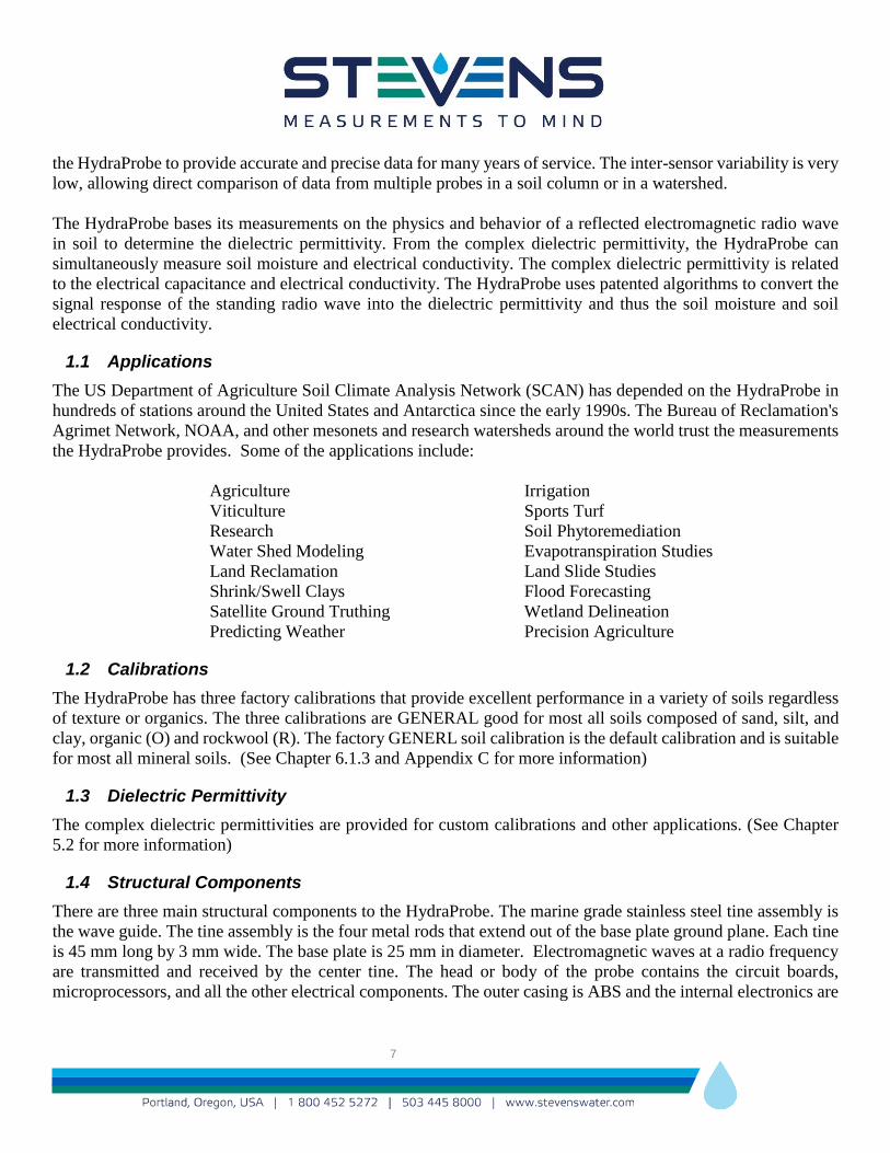
1.1 Applications
The US Department of Agriculture Soil Climate Analysis Network (SCAN) has depended on the HydraProbe in
hundreds of stations around the United States and Antarctica since the early 1990s. The Bureau of Reclamation's
Agrimet Network, NOAA, and other mesonets and research watersheds around the world trust the measurements
the HydraProbe provides. Some of the applications include:
Agriculture Irrigation
Viticulture Sports Turf
Research Soil Phytoremediation
Water Shed Modeling Evapotranspiration Studies
Land Reclamation Land Slide Studies
Shrink/Swell Clays Flood Forecasting
Satellite Ground Truthing Wetland Delineation
Predicting Weather Precision Agriculture
1.2 Calibrations
The HydraProbe has three factory calibrations that provide excellent performance in a variety of soils regardless
of texture or organics. The three calibrations are GENERAL good for most all soils composed of sand, silt, and
clay, organic (O) and rockwool (R). The factory GENERL soil calibration is the default calibration and is suitable
for most all mineral soils. (See Chapter 6.1.3 and Appendix C for more information)
1.3 Dielectric Permittivity
The complex dielectric permittivities are provided for custom calibrations and other applications. (See Chapter
5.2 for more information)
1.4 Structural Components
There are three main structural components to the HydraProbe. The marine grade stainless steel tine assembly is
the wave guide. The tine assembly is the four metal rods that extend out of the base plate ground plane. Each tine
is 45 mm long by 3 mm wide. The base plate is 25 mm in diameter. Electromagnetic waves at a radio frequency
are transmitted and received by the center tine. The head or body of the probe contains the circuit boards,
microprocessors, and all the other electrical components. The outer casing is ABS and the internal electronics are

8
permanently potted with a rock-hard epoxy resin giving the probes a rugged construction. The cable has a direct
burial casing and contains the power, ground, and data wires that are all soldered to the internal electronics.
1.5 Accuracy and Precision
The HydraProbe provides accurate and precise measurements. Table 1.1 below shows the accuracy.
Parameter Accuracy/Precision
Temperature (C) +/- 0.3 Degrees Celsius(From -30o to 60oC)
Soil Moisture wfv † (m3 m-3) +/- 0.01 to 0.03 wfv (m3 m-3) Accuracy
(Typical depends on soil)
Soil Moisture wfv † (m3 m-3) +/- 0.001 wfv (m3 m-3) Precision
Electrical Conductivity † (S/m) TUC* +/- 0.0014 S/m or +/- 1% (Typical)
Electrical Conductivity † (S/m) TC** +/- 0.0014 S/m or +/- 5% (Typical)
Real/Imaginary Dielectric Constant +/- 0.1 to 0.2 or +/- 1% FS Table 1.1 Accuracy and Precision of the HydraProbes’ Parameters.
*TUC Temperature uncorrected full scale
**TC Temperature corrected from 0 to 35o C
† The Accuracy and precision of the soil moisture, and EC measurements as well as the
temperature corrections, are highly soil dependent.
1.6 Electromagnetic Compatibility
The Stevens HydraProbe is a soil sensor that uses low power RF energy. The intended use of the HydraProbe is
to be buried in soil underground to depths ranging from 5 cm to 2 meters deep.
The HydraProbe meets and conforms to the conducted emissions criterion specified by EN 61326-1:2006 and
FCC 15.107:2010 in accordance with method CISPR 11:2009 and ANSI C63.4:2009
The HydraProbe meets the non-intentional radiator emissions, (group A) specified by EN 61326-1:2006, FCC
15.109(g) and (CISPR 22:1997):2010 in accordance with method CISPR 11:2009 and ANSI C63.4:2009 except
at 50 MHz when the probe is NOT buried as specified.
Test results are available upon request.
1.7 Configurations and Physical Specification
The HydraProbe is available in three versions, SDI-12, RS-485 and analog.
The two digital versions (SDI-12 and RS-485) incorporate a microprocessor to process the information from the
probe into useful data. This data is then transmitted digitally to a receiving instrument. SDI-12 and RS-485 are
two different methods of transmitting digital data. In both versions there are electrical and protocol specifications
that must be observed to ensure reliable data collection.

9
The Analog version requires an attached instrument to measure voltages. This information must then be processed
to generate useful information. This can be done either in the attached instrument, such as a data logger, or at a
central data processing facility.
All configurations provide the same measurement parameters with the same accuracy. The underlying physics
behind how the HydraProbe works and the outer construction are also the same for each configuration. Table
1.2 provides a physical description of the HydraProbe.
Feature Attribute
Probe Length 12.4 cm (4.9 inches)
Diameter 4.2 cm (1.6 inches)
Sensing Volume*
(Cylindrical measurement region)
Length 5.7 cm (2.2 inches)
Diameter 3.0 cm (1.2 inches)
Weight 200g (cable 80 g/m)
Power Requirements 7 to 20 VDC (12 VDC typical)
Temperature Range** -10 to 65o C
Storage Temperature Range -40 to 75o C Table 1.2 Physical description of the HydraProbe (All Versions)
*The cylindrical measurement region or sensing volume is the soil that resides between the stainless steel tine
assembly. The tine assembly is often referred to as the wave guide, and probe signal averages the soil in the
sensing volume.
** Standard temperature range is -10 to 60oC. Extended range models are available.
1.8 Soil Data Accessories and other Products
Figure 1.1. The Portable HydraGO-C and HydraGO -S allows for wireless on the go measurements of soil moisture. Connect
via Bluetooth with to smartphone with HydraGO App.

10
Figure 1.2, The eTracker Cellular Gateway can take sensor inputs directly to the cloud.
Figure 1.3. The SDI-12 Xplorer USB Adapter. For testing any SDI-12 device with a USB.
Figure 1.4. The Tempe Cell for custom calibrations, soil water retention curves

11
Part Numbers Description
63646-025 Digital HydraProbe , RS-485, W/25 FT.
63646-050 Digital HydraProbe, RS-485, W/50 FT.
63646-100 Digital HydraProbe, RS-485, W/100 FT.
93640-025 Digital HydraProbe, SDI-12, W/25 FT.
93640-050 Digital HydraProbe, SDI-12, W/50 FT.
93640-100 Digital HydraProbe, SDI-12, W/100 FT.
93640-150 Digital HydraProbe, SDI-12, W/150 FT.
93640-025-30
HydraProbe, SDI-12, 25' cable
Extended Temperature Range
93640-050-30
HydraProbe, SDI-12, 50' cable
Extended Temperature Range
93640-100-30
HydraProbe, SDI-12, 100' cable
Extended Temperature Range
93342-002 Handheld Data Reader, USB
93633-005
Field Portable with GPS, include one
HydraProbe and App
93633-006
Field Portable with W/O GPS, include
one HydraProbe and App
93669-02
HydraProbe for Field Portable 10 FT.
Cable
51139
SDI-12 XPLORER: USB TO SDI-12
Interface
92897
Cable, Analog, 7 conductor (1000'
spool)
93539
Cable, RS-485 Probe, 5 conductor
(1000' spool)
93924
Cable, SDI-12 probe, 3 conductor
(2500' spool)
93723
SDI-12 / RS-485 Multiplexer, 12
Position Table 1.3 Stevens Part numbers for HydraProbe and Accessories

12
2 Installation
2.1 Precautions
The HydraProbe is relatively easy to install depending on conditions in the field.
Avoid Damage to the HydraProbe:
● Do not subject the probe to extreme heat over 70 degrees Celsius (160 degrees Fahrenheit).
● Do not subject the probe to fluids with a pH less than 4.
● Do not subject the probe to strong oxidizers like bleach, or strong reducing agents.
● Do not subject the probe to polar solvents such as acetone.
● Do not subject the probe to chlorinated solvents such as dichloromethane.
● Do not subject the probe to strong magnetic fields.
● Do not use excessive force to drive the probe into the soil because the tines could bend. If the probe has
difficulty going into the soil due to rocks, simply relocate the probe to an area slightly adjacent.
● Do not remove the HydraProbe from the soil by pulling on the cable.
While the direct burial cable is very durable, it is susceptible to abrasion and cuts by shovels. The user should use
extra caution not to damage the cable or probe if the probe needs to be excavated for relocation.
Do not place the probes in a place where they could get run over by tractors or other farm equipment. The
HydraProbe may be sturdy enough to survive getting run over by a tractor if it is buried; however, the compaction
of the soil column from the weight of the vehicle will affect the hydrology and thus the soil moisture data.
DO NOT place more than one probe in a bucket of wet sand while logging data. More than one HydraProbe in
the same bucket while powered may create an electrolysis affect that may damage the probe.
2.2 Topographical Station Placement Considerations
The land topography often dictates the soil hydrology. Depending on the users’ interest, the placement of the
HydraProbe should represent what would be most useful. For example, a watershed researcher may want to use
the HydraProbe to study a microclimate or small hydrological anomaly. On the other hand, a farmer will want to
take measurements in an area the best represents the condition of the crops as a whole.
Other factors to consider would be tree canopy, slope, surface water bodies, and geology. Tree canopy may affect
the influx of precipitation/irrigation. Upper slopes may be better drained than depressions. There may be a shallow
water table near a creek or lake. Hill sides may have seeps or springs.
13
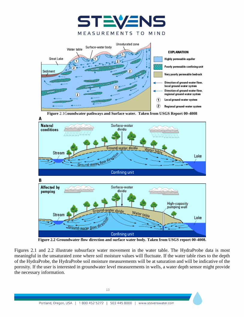
Figure 2.1Goundwater pathways and Surface water. Taken from USGS Report 00-4008
Figure 2.2 Groundwater flow direction and surface water body. Taken from USGS report 00-4008.
Figures 2.1 and 2.2 illustrate subsurface water movement in the water table. The HydraProbe data is most
meaningful in the unsaturated zone where soil moisture values will fluctuate. If the water table rises to the depth
of the HydraProbe, the HydraProbe soil moisture measurements will be at saturation and will be indicative of the
porosity. If the user is interested in groundwater level measurements in wells, a water depth sensor might provide
the necessary information.

14
2.3 Soil Sensor Depth Selection
Like selecting a topographical location, selecting the sensor depth depends on the interest of the user. Farmers
will be interested in the root zone depth while soil scientists may be interested in the soil horizons.
Depending on the crop and the root zone depth, in agriculture two or three HydraProbes may be installed in the
root zone and one HydraProbe may be installed beneath the root zone. The amount of water that should be
maintained in the root zone can be calculated by the method described in section 6. The probe beneath the root
zone is important for measuring excessive irrigation and downward water movement.
Figure 2.3 Six HydraProbes installed into 6 distinct soil horizons.
The soil horizons often dictate the depths of the HydraProbes’ placement. Soil scientist and groundwater
hydrologist are often interested in studying soil horizons. The Stevens HydraProbe is an excellent instrument for
this application because of the accuracy and precision of the volumetric water fraction calibrations. Soil horizons
are distinct layers of soil that form naturally in undisturbed soil over time. The formation of soil horizons is called
soil geomorphology and the types of horizons are indicative of the soil order (see table 2.1) Like other natural
processes, the age of the horizon increases with depth. The reason why it is so useful to have a HydraProbe in
each horizon is because different horizons have different hydrological properties. Some horizons will have high
hydraulic conductivities and thus have greater and more rapid fluctuations in soil moisture. Some horizons will
have greater bulk densities with lower effective porosities and thus have lower saturation values. Some horizons
will have clay films that will retain water at field capacity longer than other soil horizons. Knowledge of the soil
horizons in combination with the HydraProbes accuracy will allow the user to construct a more complete picture
of the movement of water in the soil. The horizons that exist near the surface can be 6 to 40 cm in thickness. In
general, with increasing depth, the clay content increases, the organic matter decreases and the base saturation
increases. Soil horizons can be identified by color, texture, structure, pH and the visible appearance of clay films.
15
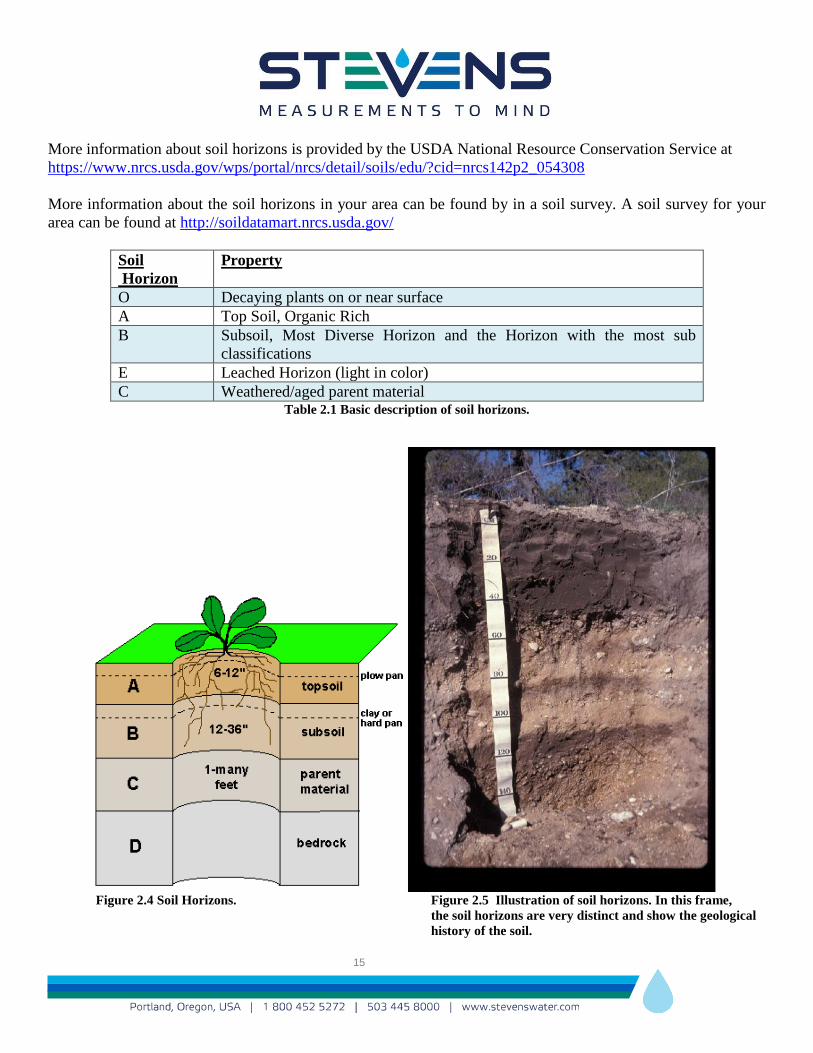
More information about soil horizons is provided by the USDA National Resource Conservation Service at
https://www.nrcs.usda.gov/wps/portal/nrcs/detail/soils/edu/?cid=nrcs142p2_054308
More information about the soil horizons in your area can be found by in a soil survey. A soil survey for your
area can be found at http://soildatamart.nrcs.usda.gov/
Soil
Horizon
Property
O Decaying plants on or near surface
A Top Soil, Organic Rich
B Subsoil, Most Diverse Horizon and the Horizon with the most sub
classifications
E Leached Horizon (light in color)
C Weathered/aged parent material Table 2.1 Basic description of soil horizons.
Figure 2.4 Soil Horizons. Figure 2.5 Illustration of soil horizons. In this frame,
the soil horizons are very distinct and show the geological
history of the soil.

16
2.4 Installation of the HydraProbe into the Soil
2.4.1 Checklist before you go into the field
Below are a list of helpful and recommended items to take into the field.
Note pad and pen
Shovel
Knife
Trowel
Tape measure
Zip ties
Screw drivers
Gloves
Water/food
Muncell Color book
Wrench
Toe tags
Wire cutter and wire strippers
Needle nose plyers
SDI-12 Xplorer
Water bottle
Rags and towels
Hand held volt meter
Marker flags
2.4.2 Test the Probes and logger in the Office before going into the Field
It is recommend to setup the logger with the sensors in the office and running the system before installing in the
field. This will allow the users to become familiar with the system and identify any problems. The HydraProbes
can be placed in water to test functionality. See section 3.1.4
2.4.3 Labeling
It is helpful to label the sensor at the head so they can be quickly identified before going in the hole. The cable at
the logger end should also be labeled. The serial number and address should be documented. The serial number
is printed on the label or use the SDI-12 “aI!” command to get the serial number.
2.4.4 Installing the HydraProbe in the Soil
The most critical considerations for the installation of the HydraProbe are that the soil should be undisturbed and
the base plate of the probe needs to be flush with the soil. To install the probe into the soil, first select the depth
(see section 2.3 for depth selection). A post-hole digger or spade works well to dig the hole. If a pit has been
prepared for a soil survey, the HydraProbes can be conveniently installed into the wall of the survey pit before it
is filled in. Use a paint scraper to smooth the surface of the soil where it is to be installed. It is important to have
the soil flush with the base plate because if there is a gap, the HydraProbe signal will average the gap into the soil
measurement and create errors.

17
Figure 2.6 HydraProbe Installed in undisturbed soil.
Push the tines of the HydraProbe into the soil until the base plate is flush with the soil. The tines should be parallel
with the surface of the ground, i.e. horizontal. Avoid rocking the probe back and forth because this will disturb
the soil and create a void space around the tines. Again, it is imperative that the bulk density of the soil in the
probe’s measurement volume remain unchanged from the surrounding soil. If the bulk density changes, the
volumetric soil moisture measurement and the soil electrical conductivity will change.
2.4.5 Soil Sensor Orientation
Figure 2.7 Horizontal placement sensor and dipping the cable is recommended
It is recommended to keep the tine assembly horizontal with the ground particularly near the surface. A drain loop
can be put in the cable to prevent water from running down the cable to the probe’s sensing area.
2.5 Wiring to a Logger Station
Connect the red wire to a +12 volt DC power supply, connect the black wire to a ground for all HydraProbe
models. The measurement duty cycle is 2 seconds.
18
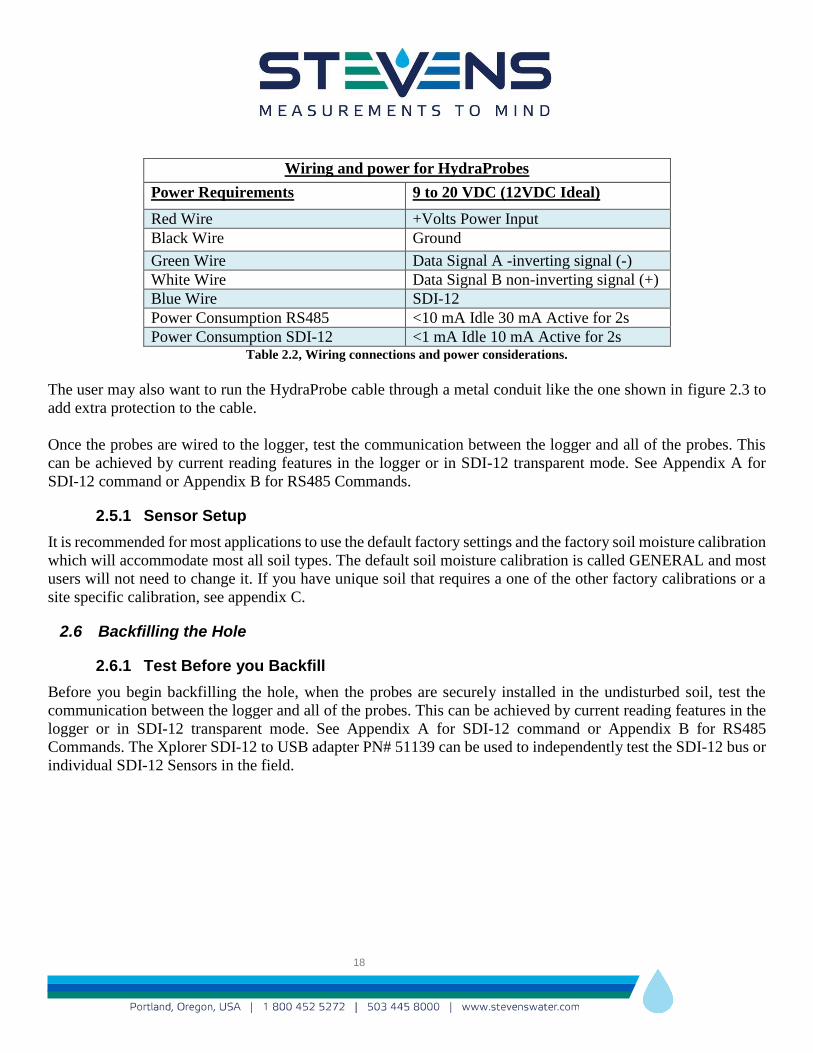
Wiring and power for HydraProbes
Power Requirements 9 to 20 VDC (12VDC Ideal)
Red Wire +Volts Power Input
Black Wire Ground
Green Wire Data Signal A -inverting signal (-)
White Wire Data Signal B non-inverting signal (+)
Blue Wire SDI-12
Power Consumption RS485 <10 mA Idle 30 mA Active for 2s
Power Consumption SDI-12 <1 mA Idle 10 mA Active for 2s Table 2.2, Wiring connections and power considerations.
The user may also want to run the HydraProbe cable through a metal conduit like the one shown in figure 2.3 to
add extra protection to the cable.
Once the probes are wired to the logger, test the communication between the logger and all of the probes. This
can be achieved by current reading features in the logger or in SDI-12 transparent mode. See Appendix A for
SDI-12 command or Appendix B for RS485 Commands.
2.5.1 Sensor Setup
It is recommended for most applications to use the default factory settings and the factory soil moisture calibration
which will accommodate most all soil types. The default soil moisture calibration is called GENERAL and most
users will not need to change it. If you have unique soil that requires a one of the other factory calibrations or a
site specific calibration, see appendix C.
2.6 Backfilling the Hole
2.6.1 Test Before you Backfill
Before you begin backfilling the hole, when the probes are securely installed in the undisturbed soil, test the
communication between the logger and all of the probes. This can be achieved by current reading features in the
logger or in SDI-12 transparent mode. See Appendix A for SDI-12 command or Appendix B for RS485
Commands. The Xplorer SDI-12 to USB adapter PN# 51139 can be used to independently test the SDI-12 bus or
individual SDI-12 Sensors in the field.

19
Figure 2.8. Xplorer SDI-12 to USB Adapter Stevens part number 51139 for testing SDI-12 bus or individual SDI-12 Sensors.
2.6.2 Backfilling Precautions
After soil is removed from the ground and piled up next to the hole, the horizons and soil become physically
homogenized. The bulk density decreases considerably because the soil structure has been disturbed. After the
probes are securely installed into the wall of the pit, the pit needs to be backfilled with the soil that came out it. It
is impossible to put the horizons back the way they have formed naturally, but the original bulk density can be
approximated by compacting the soil. For every 24 cm (1 foot) of soil put back into the pit, the soil should be
compacted. Compaction can be done by trampling the soil with feet and body weight. Mechanical compactors
can also be used, though typically they are not required. Extra care must be taken not to disturb the probes that
have exposed heads, cables and conduits when compacting the soil. If the probes were installed in a post hole, a
piece of wood, such as a post, can be used to pack the soil.
If the soil is not trampled down while it is being back filled, the compaction and bulk density of the backfill will
be considerably less than the native undisturbed soil around it. After a few months, the backfilled soil will begin
to compact on its own and return to a steady state bulk density. The HydraProbe will effectively be residing in
two soil columns. The tines will be in the undisturbed soil column, and the head, cable and conduit will be in the
backfill column that is undergoing movement. The compaction of the backfilled soil may dislodge the probe and
thus affect the measurement volume of the probe. After the probes are installed, avoid foot traffic and vehicular
traffic in the vicinity of the probes.

20
2.7 Lightning
Lightning strikes will cause damage or failure to the HydraProbe or any other electrical device, even though it is
buried. In areas prone to lightning, surge protection and /or base station grounding is recommended.
While lightning can hit the logger station, the voltage surge propagating underground can cause serious damage
to soil sensors. Underground voltage surges are called earth surge transients and the station needs to be protected
both above and below ground.
For maximum protection from lightning, attach a dual lightning dissipators to the top of the lightning rod 3 to 6
meters above the ground surface. Using at least a 1 cm thick copper cable, connect the dissipator to a series of
buried copper rod 2 cm in diameter. The buried copper rods should be at least 2 meters long buried horizontally
1.5 to 2 meters deep. Figures 2.9 and 2.10 show grounding of the soil monitoring location and the logger station.
More information can be found in the Soil Sensor Lightning Protection Guide located at
http://www.stevenswater.com/products/sensors/soil/hydraprobe/
Figure 2.9. Place grounding rods around the perimeter of the soil monitoring area

21
Place a series of grounding rods 2 to 4 meters away from the soil probes two meters deep and clamp and connect
them with a copper cable. Circle the soil sensors with the grounding rods in a way so that electrical surges
propagating through the ground will go around the soil sensors.
Figure 2.10. Ground the logger station with dual dissipators and ground rod.
22
3 Trouble Shooting and Soil Considerations
This section discuses trouble shooting and how the nature of soil can affect data. If a probe appears to be
malfunctioning, there are generally three main reasons that may explain why a probe may appear to be
malfunctioning. The three most common reasons why a probe may seem to be malfunctioning are:
1) Improper logger setup, or improper wiring,
2) Soil hydrology may produce some unexpected results, and
3) Power failure.
HydraProbes have a longevity in soil and a long warranty period, therefore; it is recommend to record the serial
numbers on the probes for support purposes.
3.1 Trouble shooting at the Logger end and Out of the ground
Section 3.1 summarizes the steps the user should take if the HydraProbe is unresponsive or outputs data that is
suspect. If the probes are in the ground, it is best to try to trouble shoot at the logger end before digging the probes
up. Keep in mind that digging the probes out of the ground can be labor intensive and may disturb the other probes
in the soil column. If the probe have to be dug out of the ground, they can be tested in water to determine if they
are functioning properly.
3.1.1 Check Wiring and Power
If the user is unable to get a response from the HydraProbe it is recommended to first physically check wire
connections from the probe to the logger. Check the cable for cuts and abrasions. A handheld voltmeter can be
used to check the voltage on the battery and the SDI-12 bus. The voltmeter can also be connected in series with
the ground wire to measure the current draw from the sensors. Idle, each HydraProbe draws 1 mA.
3.1.2 Communicate with the Sensor at the Logger End
If the logger has a current reading feature, run this feature from a laptop, app, or display that interfaces with the
logger. Try to reproduce what was observed in the logged data.
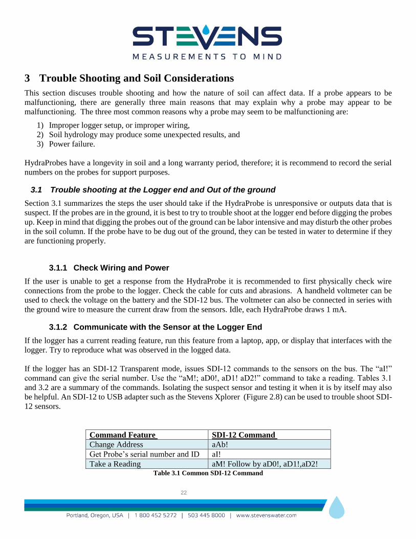
If the logger has an SDI-12 Transparent mode, issues SDI-12 commands to the sensors on the bus. The “aI!”
command can give the serial number. Use the “aM!; aD0!, aD1! aD2!” command to take a reading. Tables 3.1
and 3.2 are a summary of the commands. Isolating the suspect sensor and testing it when it is by itself may also
be helpful. An SDI-12 to USB adapter such as the Stevens Xplorer (Figure 2.8) can be used to trouble shoot SDI-
12 sensors.
Command Feature SDI-12 Command
Change Address aAb!
Get Probe’s serial number and ID aI!
Take a Reading aM! Follow by aD0!, aD1!,aD2! Table 3.1 Common SDI-12 Command

23
Table 3.2 Common M and C command for SDI-12. For RS485 commands, please see appendix B.
3.1.3 Check the Logger Configuration
If the connections are sound, the user will need to check the logger’s setup. Programming a data logger is not
always a trivial task. The data logger needs to extract the data from data ports on the logger with the desired
timing interval. The logger is often times the power source for the probes. The user may also want to cycle the
power to the probe and the logger by disconnecting and reconnecting power. Refer to the manufacturer of the
logger for tech support with the logger.
3.1.4 Remove the Suspect Probe from the Soil
If the problem cannot be resolved by checking the logger and the wiring, the probes should be dug out of the
ground, and cleaned off.
To verify that the HydraProbe is functioning properly perform the following commands: Place the HydraProbe
in distilled water in a plastic container. Make sure the entire probe is submerged. In transparent mode and with
the third parameter set (aM3!), type “1M3!” followed by “1D0!” (with a probe address of 1 for this example).
The typical response of a HydraProbe that is functioning properly should be 1+77.895+78.826+2.462. From this
example, the real dielectric permittivity is 77.895, and the imaginary dielectric permittivity is 2.462. According
to factory specifications, the dielectric constant should be from 75 to 85 and the imaginary dielectric permittivity
should be less than 5. If distilled water is not available, the user may use tap water for this procedure. It is
important to note, however, that tap water may contain trace levels of material that may affect the dielectric
permittivities readings. Isopropyl alcohol with a dielectric constant of 18.6 @20 degree C can also be used.
Common Measurement Command sets for aM! And aC!
Parameter
ordering
Parameter Unit Letter
designation
(See table)
Parameter 1 Soil Moisture Water fraction by
volume
H
Parameter 2 Bulk Electrical Conductivity with
Temperature Correction
S/m J
Parameter 3 Temperature C F
Parameter 4 Temperature F G
Parameter 5 Bulk Electrical Conductivity S/m O
Parameter 6 Real Dielectric Permittivity Unitless K
Parameter 7 Imaginary Dielectric Permittivity Unitless M

24
3.2 Soil Hydrology
Sometimes the soil moisture data may look incorrect when in fact the HydraProbes are accurately measuring the
actual soil moisture gradient. Soil Hydrology is complex and can be modeled by Darcy’s Law and Richard’s
Equation. These involved theories are beyond the scope of this manual; however, knowledge of basic soil
hydrology is worth discussing.
It’s important to note that the soil that resides between the tine assembly is where the measurements are taken. If
there is a void space in the soil between the tines, this will affect the hydrology where the HydraProbe is taking
measurements. If the void space is saturated with water, it will increase the soil moisture measurement. If the void
space is not fully saturated, the soil will appear dryer. Figure 3.1 shows the measurement volume where the
HydraProbe takes measurements and a void space between the tine assembly. These void spaces can occur from
a poor installation, such as rocking the probe side to side or not fully inserting the probe into the soil.
Figure 3.1 Measurement volume with a void space between the tine assembly.
Void spaces between the tine assembly can also occur from changing soil conditions. Factors such as shrink/swell
clays, tree roots or pebbles may introduce a void space. The following sections describe some of these and other
factors.
3.2.1 Evapotranspiration
Water in the soil will be pulled downward by gravity, however during dry periods or in arid regions, the net
movement of water is up toward the surface. Water will move upward in the soil column by a phenomenon called
Evapotranspiration (ET). ET is the direct evaporation out of the soil plus the amount of water being pulled out of
the soil by plants. Factors such as wind, temperature, humidity, solar radiation and soil type play a role in the rate
of ET. If ET exceeds precipitation, there will likely be a net upward movement of water in the soil. With the net
upward movement of soil water, ET forces dissolved salts out of solution and thus creating saline soil conditions.
25
3.2.2 Hydrology and Soil Texture
Sandy soils drain better than soils that are clay rich. In general, the smaller the soil particle size distribution, the
slower it will drain. Sometimes silt may have the same particle size distribution, as clay but clay will retain more
water for longer periods of time than silt. This can be explained by the shape of the soil particles. Clay particles
are planar whereas silt particles are spherical. Water basically gets stuck between the planar plate shaped clay
particles and thus slows the flow of water.
3.2.3 Soil Bulk Density
In general, the greater the soil density, the less water it will hold and the slower water will move through it. There
will often times be soil horizons that will be denser than others giving the soil different hydrological properties
with depth. Occasionally, water will stop or slow down and rest on a dense, less permeable layer of soil. This
phenomenon is called perched water. If two HydraProbes 20 cm apart have very different soil moisture readings,
chances are that one of the probes is residing in perched water.
There is also a relationship between soil bulk density and the complex dielectric permittivity. The soil dry bulk
density (ρb) can be described by equation [3.1]
ρb= m/V [3.1]
Where m is the mass of the dry soil in grams and V is the volume in cubic centimeters.
The bulk density is associated with the density of a soil ped or a soil core sample. The particle density (ρp ) is
the density of an individual soil particle such as a grain of sand. The two densities should not be confused with
one another. Because Er and Ei of dry soil is a function of both the bulk and particle densities (ρb, ρp ), the soil
density often creates the need for soil specific calibrations. The relationship between porosity, bulk and particle
density can be described by equation [3.2]
𝜑 = 1 −𝜌𝑏
𝜌𝑝 [3.2]
3.2.4 Shrink/Swell Clays
Shrink/swell clays belong to the soil taxonomic order vertisol and are composed of smectite clays. These clays
have a large ion exchange capacity and will shrink and swell seasonally with water content. The seasonal
expansion and contraction homogenizes the top soil and the subsoil. As the clay shrinks during a drying period,
the soil will crack open and form large crevasses or fissures. If a fissure forms in the measurement volume of the
HydraProbe, the probe will signal average the air gap caused by the fissure into the reading and potentially
generate biased results. If the fissure fills with water, the soil moisture measurement will be high, if the fissure is
dry, the soil moisture measurement will be lower than expected. If the HydraProbe measurements are being
affected by shrink/swell clays, it is recommend to relocate the probe to an adjacent location.

26
3.2.5 Rock and Pebbles
Often times, it will be obvious if a rock is encountered during an installation. Never use excessive force to insert
the probe into the soil. Some soils will have a distribution of pebbles. If a pebble finds its way between the probe’s
tines, it will create an area in the measurement volume that will not contain water. The probe will signal average
the pebble and thus lower the soil moisture measurement. If the pebble is an anomaly, relocating of the probe
would provide more representative soil measurements. However, if it is revealed from the soil survey that there
exists a random distribution of pebbles, a pebble between the tines may provide realistic measurements because
of the way pebbles influence soil hydrology.
3.2.6 Bioturbation
Organisms such as plants and burrowing animals can homogenize soil and dislodge soil probes. A tree root can
grow between the tines affecting the measurements and in some cases, tree roots can bring a buried soil probe to
the soil surface. Burrowing mammals and invertebrates may decide that the HydraProbes’ tine assembly makes
an excellent home. If the HydraProbe’s tine assembly becomes home to some organism, the soil moisture
measurements will be affected. After the animal vacates, the soil will equilibrate and the soil measurements will
return to representative values.
The cable leading to the probe may also become a tasty treat for some animals. If communication between the
logger and the probe fails, check the cable for damage. A metal conduit like the one shown in figure 2.3 is
recommended.
3.2.7 Salt Affected Soil and the Loss Tangent
The HydraProbe is less affected by salts and temperature than TDR or other FDR soil sensors because of the
delineation of the dielectric permittivity and operational frequency at 50 Mhz. While the HydraProbe performs
relatively well in salt affected soils, salts that are dissolved in the soil water will influence both dielectric
permittivities ts and thus the measurements. The salt content will increase the imaginary dielectric constant and
thus the soil electrical conductivity. See Chapter 4. The HydraProbe will not measure electrical conductivity or
soil moisture beyond 1.5 S/m
In general, if the electrical conductivity reaches 1 S/m, the soil moisture measurements will be significantly
affected. The imaginary dielectric constant will have an influence on the real dielectric constant because dissolve
cations will inhibit the orientation polarization of water. When addressing the HydraProbes’ performance in salt
affected soil, it is useful to use the loss tangent equation [3.3].
𝑇𝑎𝑛 𝛿 =𝜀𝑖
𝜀𝑟 [3.3]
The loss tangent (Tan δ) is simply the imaginary dielectric constant divided by the real dielectric constant. If Tan
δ becomes greater than 1.5 than the HydraProbes calibration becomes unreliable. It is interesting to note that the
HydraProbe will still provide accurate dielectric constant measurements up to 1.5 S/m. If the salt content reaches
27
a point where it is affecting the calibrations, the user can use a custom calibration that will still provide realistic
soil moisture measurements in the most salt affected soils. See Appendix C for custom calibrations.
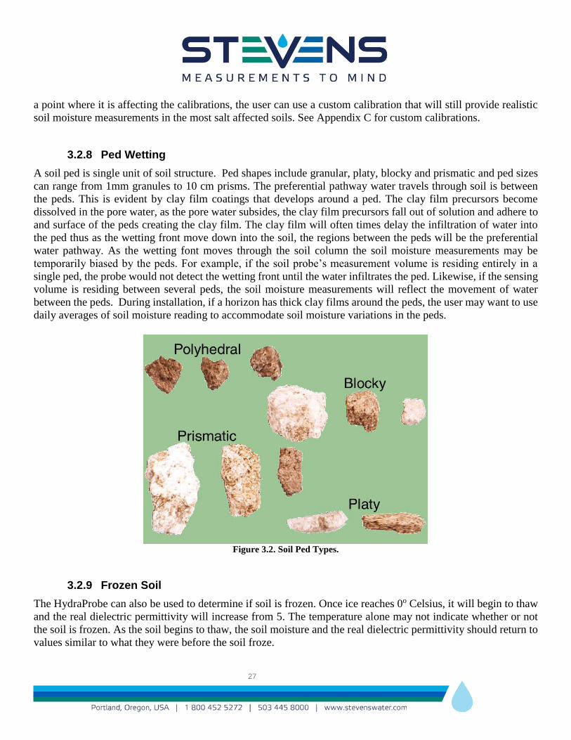
3.2.8 Ped Wetting
A soil ped is single unit of soil structure. Ped shapes include granular, platy, blocky and prismatic and ped sizes
can range from 1mm granules to 10 cm prisms. The preferential pathway water travels through soil is between
the peds. This is evident by clay film coatings that develops around a ped. The clay film precursors become
dissolved in the pore water, as the pore water subsides, the clay film precursors fall out of solution and adhere to
and surface of the peds creating the clay film. The clay film will often times delay the infiltration of water into
the ped thus as the wetting front move down into the soil, the regions between the peds will be the preferential
water pathway. As the wetting font moves through the soil column the soil moisture measurements may be
temporarily biased by the peds. For example, if the soil probe’s measurement volume is residing entirely in a
single ped, the probe would not detect the wetting front until the water infiltrates the ped. Likewise, if the sensing
volume is residing between several peds, the soil moisture measurements will reflect the movement of water
between the peds. During installation, if a horizon has thick clay films around the peds, the user may want to use
daily averages of soil moisture reading to accommodate soil moisture variations in the peds.
Figure 3.2. Soil Ped Types.
3.2.9 Frozen Soil
The HydraProbe can also be used to determine if soil is frozen. Once ice reaches 0o Celsius, it will begin to thaw
and the real dielectric permittivity will increase from 5. The temperature alone may not indicate whether or not
the soil is frozen. As the soil begins to thaw, the soil moisture and the real dielectric permittivity should return to
values similar to what they were before the soil froze.
28
4 Theory of Operation, Dielectric Permittivity and Soil Physics.
4.1 Introduction
Analytical measurement of soil moisture and matric potential are represented by a number of different
technologies on the market. Described here is the theory behind electromagnetic soil sensors and a brief
discussions of matric potential. Soil moisture can be expressed as a gravimetric water fraction, a volumetric water
fraction (θ, m3 m-3) or as a capillary matric potential (ψ, HPa). Soil sensors that employ electromagnetic waves
(dielectric permittivity based) to estimate soil moisture typically express the soil water content as volumetric
fraction, where sensors measuring soil water potential output units of pressure or the log of the pressure (pF).
4.2 Soil Matric Potential
Capillary matric potential sometimes referred to as tension or pressure head (ψ, hPa) is the cohesive attractive
force between a soil particle and water in the pore spaces in the soil particle/water/air matrix. Typical ranges are
0 to 10,000,000 hPa where 0 is near saturation and 10,000,000 hPa is dryness. The drier the soil the more energy
it takes to pull water out of it. Capillary forces are the main force moving water in soil and it typically will move
water into smaller pores and into drier region of soil. This process is also called wicking.
Because of the wide pressure ranges that can be observed from very wet to very dry conditions, matric potential
is often express as the common log of the pressure in hPa. The log of the pressure is called pF. For example
1,000,000 hPa is equal to a pF of 6..
Water potential is highly texture dependent. Clay particles have a larger surface area and thus will have a higher
affinity for water than that of silt or sandy soils. The most common methods for measuring or inferring the matric
potential including granular matrix sensors such as gypsum electrical resistance blocks, and tensiometers which
measure pressure directly.
Heat dissipation type matric potential sensors measure the matric potential indirectly by measuring the heat
capacitance of a ceramic that is in equilibrium with the soil. With heat up and cool down cycles of heating
elements in the ceramic, the heat capacitance can be calculated which in turn is calibrated to the matric potential.
Heat capacitance based matric potential sensors offer advantages in accuracy, range and maintenance over other
technologies. The Stevens TensioMark pF Sensor (part number 51133-200) is a highly accurate SDI-12 matric
potential sensor that uses heat capacitance technology
Matric potential is important for irrigation scheduling because it can represent the soil water that would be
available to a crop. Many unsaturated flow models require a soil water retention curve where water fraction by
volume is plotted with the matric potential in a range of moisture conditions (Figure 4.2).A soil water retention
curve can help understand the movement and distribution of water such as infiltration rates, evaporation rates and
water retentions (Warrick 2003). Table 4.1 shows the general values of matric potential under different
hydrological thresholds and soil textures.

29
Figure 4.1. TensioMark SDI-12 heat capacitance based Matric Potential Sensor. (PN 51133-200)
Figure 4.2. Soil Water Retention Curve. Soil matric potential verse soil moisture.
Soil Condition Matric Potential Soil Moisture %
Bar kPa hPa PSI ATM pF Sand Silt Clay
Saturation 0 0 0 0 0 42% 40% 55%
0.2 20 200 2.9007 0.197 2.30
Field Capacity 0.33 33 330 4.7862 0.326 2.52 10% 30% 40%
1 100 1000 14.503 0.987 3
Permanent Wilting Point 15 1500 15000 217.55 14.80 4.18 4 15% 21% Table 4.1. General trends of matric potentials under different soil hydrologic conditions and textures
30
4.3 Electromagnetic Soil Water Methods and Soil Physics
The behavior of electromagnetic waves from 1 to 1000 MHz in soil can be used to measure or characterize the
complex dielectric permittivity. Dielectric permittivity was first mathematically quantified by Maxwell’s
Equations in 1870s. In the early 1900s, research with radio frequencies led to modern communication and the
arrival of the television in the 1950s. In 1980, G. C. Topp (Topp 1980) proposed a method and a calibration to
predict soil moisture based on the electrical properties of the soil known as the Topp Equation. Today, there are
dozens of different kinds of soil moisture sensors commercially available that in one way or another base their
soil moisture estimation on the dielectric permittivity. Among all of the electronic soil sensors commercially
available, measurement involving the complex dielectric permittivity remains the most practical way to determine
soil water content from an in situ sensor or portable device. Electromagnetic soil sensors use an oscillating radio
frequency and the resultant signal is related to the dielectric permittivity of the soil where the in situ soil
particle/water/air matrix is the dielectric. Subsequent calibrations then take the raw sensor response to a soil
moisture estimation.
4.3.1 Dielectric Theory
Complex dielectric permittivity describes a material’s ability to permit an electric field. As an electromagnetic
wave propagates through matter, the oscillation of the electric field is perpendicular to the oscillation of the
magnetic field and these oscillations are perpendicular to the direction of propagation. The dielectric permittivity
of a material is a complex number containing both real and imaginary components and is dependent on frequency,
temperature, and the properties of the material. This can be expressed by,
ir j * [4.1]
where К* is complex dialectic permittivity, εr is the real dielectric permittivity, εi is the imaginary dielectric
permittivity and 1j (Topp 1980). As the radio wave propagates and reflects through soil, the properties and
water content of the soil will influence the wave. The water content, and to a less extent the soil properties will
alter and modulate electromagnet radio signal as it travels through the soil by changing the frequency, amplitude,
impedance and the time of travel. The Dielectric permittivity can be determined by measuring these modulations
to the radio frequency as it propagates through the soil. In general, the real component represents energy storage
in the form of rotational or orientation polarization which is indicative of soil water content. The real dielectric
constant of water is 78.54 at 25 degrees Celsius and the real dielectric permittivity of dry soil is typically about
4. Changes in the real dielectric permittivity are directly related to changes in the water content and all
electromagnetic soil sensors base their moisture calibrations on either a measurement or estimation of the real
dielectric permittivity of the soil particle/water/air matrix. (Jones 2005, Blonquist 2005). The imaginary
component of the dielectric permittivity,
v
dcreli
f
2 [4.2]

31
represents the energy loss where εrel is the molecular relaxation, f is the frequency, εv permittivity of a vacuum,
and σdc is DC electrical conductivity. In most soils, εrel is relatively small and a measurement of the imaginary
component yields a good estimation of the electrical conductivity from 1 to 75 MHz (Hilhorst 2000). In sandy
soils, the molecular relaxation can be negligible. The HydraProbe estimates electrical conductivity by measuring
the imaginary and rearranging equation [4.2] based on the assumption that the relaxations are near zero.
The storage of electrical charge is capacitance in Farads and is related to the real component (non-frequency
dependent) by
C = gε εv [4.3]
Where g is a geometric factor and ε is the dielectric constant. If the electric field of the capacitor is oscillating
(i.e. electromagnetic wave), the capacitance also becomes a complex number and can be describe in a similar
fashion as the complex dielectric permittivity in equations [4.1] and [4.2] (Kelleners 2004).
The apparent dielectric permittivity εa, is a parameter that contains both the real and the imagery dielectric
permittivities and is the parameter used by most soil sensors to estimate soil moisture.
εa = {1+[1+tan2(εi/εr)]1/2}εr/2 [4.4]
From equation [4.4], the apparent dielectric permittivity is a function of both real and imaginary components
(Logsdon 2005). High values of εi will inflate the εa which may cause errors in the estimation of soil moisture
content. In an attempt to shrink the errors in the moisture calibration from the εi, some soil sensors such as time
domain reflectometry will operate at high frequencies giving the εa more real character. In practice, soils high in
salt content will inflate the soil moisture measurement because εa will increase due to the DC conductivity
component of εi. Also, the εi is much more sensitive to temperature changes than εr creating diurnal temperature
drifts in the soil moisture data (Blonquist 2005, Seyfried 2007). The soil moisture sensors that can best isolate the
real component and delineate it from the imaginary will be the most accurate and will have a lower inter-sensor
variability.
Water is a polar molecule, meaning that one part of the water molecule caries a negative charge while the other
half of the molecule caries a positive charge. While water is very polar, soils are rather non-polar. The polarity of
water causes a rotational dipole moment in the presence of an electromagnetic wave while soil remains mostly
uninfluenced. This means that water will rotate and reorientate with the rise and fall of the oscillating electric
field i.e. electromagnetic wave while soil remains mostly stationary. From 1 to 1000 MHz, the water rotational
dipole moment of water will occur at the same frequency of the electromagnetic wave. It is this rotational dipole
moment of water that is responsible for water’s high dielectric constant1 of about 80. Dry Soil will have a dielectric
constant of about from about 4 to 5. Large changes in the dielectric permittivity will are directly correlated to
changes in soil moisture. Figure 4.2 shows the polarity of a water molecule and how it can reorient itself in
response to electromagnetic oscillations.
1Terminology note. The term “real dielectric constant” generally refers to a physical property that is constant at a specified condition. The term “real
dielectric permittivity” or “real permittivity” refers to the real dielectric constant of a media that is undergoing change, such as soil.

32
Figure 4.3. A water molecule in the liquid phase reorienting i.e. rotational dipole moment.
Figure [4.3] illustrates the different kinds of polarizations exhibited by most materials. Soils will have space
charge and atomic polarizations while water will re-orientate.
Figure [4.4]. Illustration of polarization. The real dielectric permittivity of soil is mostly due to orientation polarization of
water (Taken from Lee et al. 2003)
4.3.2 Temperature
Both the real and imaginary dielectric permittivities will be influenced by temperature. The imaginary component
is much more sensitive to changes in temperature than the real component. (Seyfried 2007).
4.3.3 Temperature and the Real Permittivity
The real dielectric permittivity of water will have a slight dependence on temperature. As the temperature
increases, molecular vibrations will increase. These molecular vibrations will impede the rotational dipole
moment of liquid water in the presents of an osculating electric field; consequently, the real dielectric permittivity
of water will decrease as the temperature increases. The empirical relationship with temperature found in the
literature is show in equation [4.5] (Jones 2005)
εr,w(T) = 78.54[1-4.579X10⁻³ (T-298)+ 1.19 X10⁻⁵ (T-298)2-2.8X10⁻⁸(T-298)3] [4.5]
While the HydraProbe has a temperature corrections for the electrical components on the circuit board, the factory
calibrations do not apply a temperature correction to the measured soil moisture values. Water in liquid form will
have its dielectric constant decrease with increasing temperature, but in soil, water’s dielectric dependency with

33
temperature is more complicated due to bound water affects. As temperature changes, the molecular vibrations
of the water and cations that are bonded to soil particles at a microscopic level can affect the dipole moments in
the presence of a radio frequency. In practical terms, temperature correction to soil moisture calibrations are
highly soil dependent. In some soils, the real dielectric can trend downward with increasing temperature as it does
in liquid form, or it can trend upward with increasing temperature (Seyfried 2007).
4.3.4 Temperature and the imaginary permittivity
The imaginary permittivity is highly temperature dependent and the temperature dependence is similar to that of
the bulk electrical conductivity.
4.4 Types of Commercial Electromagnetic Soil Sensors
There are dozens of different kinds of electronic soil sensors commercially available and it can be confusing to
understand the different technologies. Table 4.2 summarizes the types of sensing methods.
Method Physical Measurement Basis for Soil Moisture Typical
Frequency
TDR Time of travel of a reflected wave Apparent Permittivity 1000 MHz
TDT Time of travel Apparent Permittivity 150 to
2000 MHz
Capacitance
(Frequency)
Shift in Frequency
(Resonance Frequency)
Apparent Permittivity 150 MHz
Capacitance
(Charge)
Capacitor Charging time Capacitance NA
Differential
Amplitude
Difference in reflected amplitudes Apparent Permittivity 75 MHz
Ratiometric
amplitude
Impedance
Ratio of reflected amplitudes to
measure the impedance.
Real Dielectric Permittivity 50MHz
Table 4.2. Summary of commercially available soil sensing methods
Both time domain reflectometry (TDR and time domain transmission (TDT) use the time of travel of the radio
wave to measure the apparent permittivity (Blonquist 2005-A). The primary difference between TDR and TDT
is TDR characterizes the reflected wave where as TDT characterizes the travel time on a wave guide of a set path
length.
Capacitance can be measured from the change in frequency from a reflected radio wave or resonance frequency
(Kelleners 2004). These sensors are often referred to as frequency domain reflectometers (FDR), however the
term FDR is often misused because most frequency sensors are using a single frequency and not a domain of
frequencies. Other capacitance probes and amplitude impedance-based probes are often mistakenly referred to as
“FDRs”.

34
The capacitance of a parallel plate capacitor can be measured from the time it takes to charge the capacitor. Some
commercially available soil sensors can measure the capacitance of the soil from the time of charge and then
calibrate for soil moisture.
Another method for determining the apparent permittivity is measuring the difference between the incident
amplitude and the reflected amplitude (Gaskin 1996).
4.4.1 The HydraProbe, a Ratiometric Coaxial Impedance Dielectric Reflectometer
The Stevens HydraProbe is different than other soil sensing methods. It characterizes the ratio of the amplitudes
of reflected radio waves at 50 MHz with a coaxial wave guide. A numerical solution to Maxwell’s equations first
calculates the complex impedance of the soil and then delineates the real and imaginary dielectric permittivity
(Seyfried 2004, Campbell 1990). The mathematical model that delineates the real and imaginary component from
the impedance of the reflected signal resides in the microprocessor inside the digital HydraProbe. These
computations are based on the work of J. E. Campbell at Dartmouth College (Campbell 1988, Campbell 1990,
Kraft 1988).
The HydraProbe from an electric and mathematical prospective can be referred to ratiometric coaxial impedance
dielectric reflectometer and works similar to a vector network analyzer at a single frequency. The term
“ratiometric” refers to the process by which the ratio of the reflected signal over incident signal is first calculated
which eliminates any variability in the circuit boards from one probe to the next. This step is performed on several
reflections. The term “coaxial” refers to the metal wave guild that get inserted into the soil. It has three outer
tines with a single tine in the middle that the both receives and emits a radio frequency at 50 MHz. “Impedance”
refers to the intensity of the reflected signal, and “dielectric reflectometer” refers to a reflected signal that is used
to measure a dielectric.
4.4.2 Advantages of using the real dielectric permittivity over the apparent permittivity
Unlike most other soil sensors, the HydraProbe measures both the real and the imaginary components of the
dielectric permittivity as separate parameters. The HydraProbe bases the soil moisture calibration on the real
dielectric permittivity while most other soil moisture technologies base their soil moisture estimation on the
apparent permittivity which is a combination of the real and imaginary components as defined in equation [4.4]
(Logsdon 2010). Basing the soil moisture calibration on the real dielectric permittivity instead of the apparent
permittivity has many advantages. Because the HydraProbe separates the real and imaginary components, the
HydraProbe’s soil moisture calibrations are less affected by soil salinity, temperature, soil variability and inter
sensor variability than most other electronic soil sensors.
4.4.3 The HydraProbe is Easy to Use
Despite the complexities of the mathematics the HydraProbe performs, the duty cycle including the warmup time,
the processing of the signals, and the mathematical operations being performed by the microprocessor takes under
two seconds. The user can connect the sensor to a logger or other reading device with Plug-&-Play ease while
maintaining a high level of confidence in the data.
35
5 Measurements, Parameters, and Data Interpretation
5.1 Soil Moisture
5.1.1 Soil Moisture Units
The HydraProbe provides accurate soil moisture measurements in units of water fraction by volume
(wfv or m3m-3) and is symbolized with the Greek letter theta “θ”. Soil moisture is parameter “H” on the digital
HydraProbe. Multiplying the water fraction by volume by 100 will equal the volumetric percent of water in soil.
For example, a water content of 0.20 wfv means that a 1000 cubic centimeters soil sample contains 200 cubic
centimeters water or 20% by volume. Full saturation (all the soil pore spaces filled with water) occurs typically
between 0.35-0.55 wfv for mineral soil and is quite soil dependent.
There are a number of other units used to measure soil moisture. They include % water by weight, % available
(to a crop), and inches of water to inches of soil, % of saturation, and tension (or pressure). It is important to have
an understanding of the different water to express soil moisture and the conversion between units can be highly
soil dependent.
Because the bulk density of soil is so highly variable, soil moisture is most meaningful as a water fraction by
volume or volumetric percent. If weight percent were used, it would represent a different amount of water from
one soil texture to the next and it would be very difficult to make comparisons. .
5.2 Soil Moisture Measurement Considerations for Irrigation
Soil moisture values are particularly important for irrigation optimization and to the health of a crop. There are
two different approaches for determining an irrigation schedule from soil moisture data, the fill point method and
the mass balance method. Other common irrigation scheduling methods that do not include soil moisture sensors
use evapotranspiration (ET). ET is the rate of water leaving the soil by the combination of direct evaporation of
water out of the soil and the amount of water being transpired by the crop. ET can be thought of as negative
precipitation. ET is determined from calculations based on metrological conditions such as air temperature , solar
radiation and wind. The most common ET irrigation scheduling determination is called the Penman-Monteith
Method publish in FAO-56 1998 Food and Agriculture Organization of the UN. The FAO 56 method is also a
mass balance approach where the amount of water that is leaving the soil can be determined and matched by the
irrigation schedule. In practice to ensure the success of the crop, ET methods in combination with soil sensor data
can be used by irrigators to best manage irrigation.
5.2.1 Fill Point Irrigation Scheduling
The fill point method is qualitative in that the irrigator looks at changes in soil moisture. With experience and
knowledge of the crop, an irrigation schedule can be developed to fill the soil back up to a fill point. The fill point
is an optimal soil moisture value that is related to the soil’s field capacity. The fill point for a particular sensor is
determined by looking at soil moisture data containing a number of irrigation events. This can be an effective and
simple way to optimize irrigation. Because it is qualitative, accuracy of the soil moisture sensor is less important

36
because the fill point is determined by looking at changes in soil moisture and not the actual soil moisture itself.
This in some ways can be more efficient because lower cost soil moisture sensors can be used without calibration.
While the fill point method can be easy to implement and is widely used for many crops, the mass balance method
however can better optimize the irrigation, better control salinity build up, and minimize the negative impacts of
over irrigation.
5.2.2 Mass Balance Irrigation Scheduling
The mass balance method or sometimes called scientific irrigation scheduling is an irrigation schedule determined
by calculating how much the water is needed based on accurate soil moisture readings and from the soil properties.
Equations [5.1], [5.2] and [5.3] can help to determine how much water to apply. The following are terms
commonly used in soil hydrology:
● Soil Saturation, (θSAT) refers to the situation where all the soil pores are filled with water. This occurs
below the water table and in the unsaturated zone above the water table after a heavy rain or irrigation
event. After the rain event, the soil moisture (above the water table) will decrease from saturation to field
capacity.
● Field Capacity (θFC in equations below) refers to the amount of water left behind in soil after gravity drains
saturated soil. Field capacity is an important hydrological parameter for soil because it can help determine
the flow direction. Soil moisture values above field capacity will drain downward recharging the
aquifer/water table. Also, if the soil moisture content is over field capacity, surface run off and erosion
can occur. If the soil moisture is below field capacity, the water will stay suspended in between the soil
particles from capillary forces. The water will basically only move upward at this point from evaporation
or evapotranspiration.
● Permanent Wilting Point (θPWP) in equations below) refers to the amount of water in soil that is unavailable
to the plant.
● The Allowable Depletion (θAD in the equations below) is calculated by equation [5.1]. The allowable
depletion represents the amount of soil moisture that can be removed by the crop from the soil before the
crop begins to stress.
● Lower soil moisture Limit (θLL from [5.3]) is the soil moisture value below which the crop will become
stressed because it will have insufficient water. When the lower limit is reached, it is time to irrigate.
● The Maximum Allowable Depletion (MAD) is the fraction of the available water that is 100% available
to the crop. MAD can depend on soil or crop type.
● Available Water Capacity (θAWC) is the amount of water in the soil that is available to the plant.
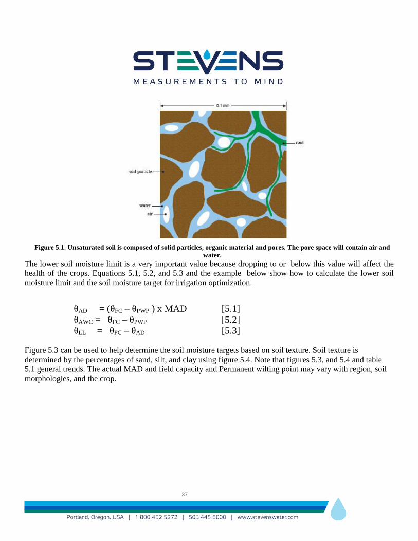
37
Figure 5.1. Unsaturated soil is composed of solid particles, organic material and pores. The pore space will contain air and
water.
The lower soil moisture limit is a very important value because dropping to or below this value will affect the
health of the crops. Equations 5.1, 5.2, and 5.3 and the example below show how to calculate the lower soil
moisture limit and the soil moisture target for irrigation optimization.
θAD = (θFC – θPWP ) x MAD [5.1]
θAWC = θFC – θPWP [5.2]
θLL = θFC – θAD [5.3]
Figure 5.3 can be used to help determine the soil moisture targets based on soil texture. Soil texture is
determined by the percentages of sand, silt, and clay using figure 5.4. Note that figures 5.3, and 5.4 and table
5.1 general trends. The actual MAD and field capacity and Permanent wilting point may vary with region, soil
morphologies, and the crop.

38
Soil Saturation θSAT Field Capacity θFC Permanent Wilting Point θpw
Figure 5.2. Hydrological conditions of soil.
Crop Maximum Allowable
Depletion (MAD)
Effective Root
Depth (Inches)
Grass 50% 7
Table beet 50% 18
Sweet Corn 50% 24
Strawberry 50% 12
Winter Squash 60% 36
Peppermint 35% 24
Potatoes 35% 35
Orchard Apples 75% 36
Leafy Green 40% 18
Cucumber 50% 24
Green Beans 50% 18
Cauliflower 40% 18
Carrot 50% 18
Blue Berries 50% 18 Table 5.1, Typical Maximum Allowable Depletion based on crop. Effective Root Zone Depth. Taken from Smesrud 1998. Note
that these values may be region or crop type specific.

39
Figure 5.3 soil textures and the available water.
Texture Clay Silty
Clay
Clay
Loam
Loam Sandy
Loam
Loamy
Sand Sand
MAD 0.3 0.4 0.4 0.5 0.5 0.5 0.6 Table 5.2, Maximum allowable depletions for different soil textures.

40
Figure 5.4. Soil textural triangle.
Example of an Irrigation scheduling based on soil moisture values:
How much water should be applied? The soil is a silt, the MAD is 50%, and the soil moisture is 20% throughout
the root zone which is down to 24 cm. The sprinkler is 75% efficient.
Answer: From tables 5.1 and 5.2 the MAD = 0.5, From Figure 5.3 (or a soil surrey) θPWP = 16% and the field capacity,
θFC is 32%. Therefor using equations 5.1 to 5.3, the optimal soil moisture is 24 to 32%. θFC – θ = 32% - 16% =
16%. Therefor the soil needs to be irrigated to increase the soil moisture by 16% down to 24 cm, 16% X 24 cm =
3.8 cm of water need to be added. If the sprinkler is 75% efficient than 3.8 cm/0.75 = 5.12 cm of water should be
applied. Note the rate of water coming out of the sprinkler should not exceed the infiltration rate of the soil and
the run time of the sprinklers would depend on the specification of the sprinkler.

41
5.2.3 Soil Moisture Calibrations
The soil moisture calibration is an estimation of the soil moisture from a mathematical equation that contains the
real dielectric permittivity (Topp 1980). The HydraProbe has 3 factory calibrations to choose from and custom
calibration features in case a specific site calibration is necessary. The factory GENERAL or GEN calibration
is the best general purpose calibration available and is the default calibration on the HydraProbe’s firmware. The
GEN calibration is based on research conducted by the US Department of Agriculture, Agricultural Research
Service (Seyfried 2005) and is the standard calibration for the US Department of Agriculture’s SNOTEL, SCAN
networks and NOAA’s Climate Reference Network. The factory default GEN calibration is equation [A2] in the
appendix C where A = 0.109, B = -0.179 and εr is the raw real dielectric permittivity.
It is recommended to keep the HydraProbe set to the default calibration. If the soil requires a custom calibration
or if further validation of the calibration is needed, the real dielectric permittivity (Parameter 6 on “aM!, aC!) can
be logged until a new calibration can be developed. See appendix C for more information about calibration
validation and development.
5.2.3.1 Other Factory Calibration
In addition to the factory General Calibration, the HydraProbe has an Organic soil calibration, O, and a rockwool
calibration, R. See appendix C for information on the calibration settings. The user may want to validate the
factory calibration to make sure it has suitable accuracy for a specific soil. If the factory calibration is off, the user
may develop a new soil specific calibration. A new soil specific calibration can be developed through gravimetric
analyses. It is recommended to log the real dielectric permittivity (Parameter 6 on “aM!, aC!). If a new calibration
is developed, the historical data set can be recalibrated if the data set contains the raw real dielectric permittivity
value. Individual sensors do not need their own calibration. Because all HydraProbes measure the same way with
extremely low variability from sensor to sensor, the same calibration formula can be applied to any HydraProbe.
5.3 Soil Salinity and the HydraProbe EC Parameters
Soil bulk electrical conductivity (EC) is important for assessing the salinity of the soil and soil pore water.
Temperature corrected EC is the second parameter in “aM!,aC!” And the raw un-corrected electrical conductivity
and is the 5th parameter in “aM!, aC!” in the SDI-12 parameter sets. Electrical conductivity also referred to as
specific conductance and is measured in Siemens/meter (S/m). Siemens is inversely related to resistance in Ohms
(Siemens = 1/Ohms) and represents a materials ability to conduct an electric current. There are a number of related
units for EC. Table 5.3 below summarizes the unit conversion.
The electrical conductivity parameters are calculated from the imaginary dielectric permittivity by rearranging
equation [4.2]. The calculation of EC is based on the assumption that the molecular relaxations are negligible or
very small. This assumption provides a good approximation for EC in sandy or silty soils where molecular
relaxations are minimal. The approximation of EC from the imaginary permittivity in clay rich soils however will
be less accurate due to the possible presents of molecular relaxations. While the accuracy of the EC parameters
in soil are highly soil dependent, the HydraProbe’s EC measurements in slurry extracts, water samples, and
aqueous solutions will be accurate (<+/- 1 to 5%) up to 0.3 S/m. Because EC can be sensitive to changes in
temperature, a temperature correction is provided.

42
Convert to →
Convert From ↓
S/m dS/m mS/m μS/m S/cm dS/cm mS/cm μS/cm
S/m 1 10 1000 1E6 0.01 0.1 10 10000
dS/m 0.1 1 100 1E5 .001 0.01 1 1000
mS/m 0.001 0.01 1 1000 1E-5 0.0001 0.01 10
μS/m 1E-6 1E-5 0.001 1 1E-8 1E-7 0.00001 0.01
S/cm 100 1000 1E5 1E8 1 10 1000 1E6
dS/cm 10 100 10000 1E7 0.1 1 100 1E5
mS/cm 0.1 1 100 100000 0.001 0.01 1 1000
μS/cm 0.0001 0.001 0.1 100 1E-6 1E-5 0.001 1 Table 5.3. Convert EC units on the left to the EC units on top by multiplying by the factor. For example
2 dS/m X 0.1 = 0.2 S/m
5.3.1 Soil Salinity
The soil salinity is salt build up in the soil and can be caused by poor drainage, poor irrigation water quality and
salt water intrusion in coastal areas. Salt or specifically the dissolve ions in solution are the primary component
of the soil matrix that conducts electricity. While the EC parameter is highly dependent on the level of soil salinity,
it will also rise and fall with soil moisture. The buildup of salinity in the soil is typically not beneficial to crops,
grasses or the microbial community in the soil. The soil salinity may also affect the soil hydrology. Plant diseases
and pathogens, and reduced crop yields or even crop failures may occur from excessive soil salinity therefore,
monitoring the soil salinity will help ensure the health of crops.
Soil salinity is dissolved salts such as sodium chloride, calcium chloride and magnesium chloride. The salts may
not only be chlorides but carbonates as well. Fertilizers such as nitrates do not have a strong conductivities
therefore the EC measured in a soil is primarily going to be attributed to the sodium and soil moisture.
5.3.2 Bulk EC versus Pore Water EC
The EC in soil is more complex than it is in a water sample and can be difficult and confusing to interpret. The
bulk soil electrical conductivity σb is the EC of the undisturbed soil/water/air matrix and is the parameter measured
by the HydraProbe. It is important not to confuse the bulk EC with the soil pore water EC, σp. The soil pore water
EC is the electrical conductivity of the water in the pore spaces of the soil. Because the pore water EC may be
difficult to directly measure, a soil slurry can be prepared by taking one part dry soil and two parts distilled water
and measuring the EC of the water extract from the slurry. The EC of the extract (ECe or σe) is the parameter
traditionally found in soil science or agriculture literature because is relativity easy to measure and provides an
“apples to apples” comparison of soil salinity conditions. The HydraProbe can be used to measure the ECe if
properly placed in the watery extract.

43
5.3.3 Bulk EC and EC Pathways in Soil
Soil is a matrix that is basically composed of solid material, water in the pore spaces and air. In situ soil sensors
(soil sensors in the ground) measure the dc bulk electrical conductivity (σb) which is the electrical conductivity
of the soil/water/air matrix combined. Figure [5.3] shows the three pathways the electrical conductivity can
propagate in soil. The bulk density, the porosity, the tortuosity, the water content, and the dissolved ion
concentration working in concert with the different pathways, dramatically influences the bulk electrical
conductivity of a soil.
Pathway 1 is the electrical pathway that goes from water to the soil and back through the water again. The
electrical conductivity contribution of pathway 1 is a function of the conductivity of the water and soil. As water
increases, the electrical conduit of pathway 1 increases which may increase the electrical conductivity of the soil
as a whole.
Pathway 2 is the pathway that is attributed to the electrical conductivity of the just the water in the soil pores.
Increasing the dissolved salts will increase the conductivity of pathway 2; however, like pathway 1, increases in
the soil water content will increase the size of the pathway thus increasing the overall bulk electrical conductivity.
That is to say, that there are two factors influencing the electrical conductivity of pathway 2, namely the dissolved
salt concentration and the size of the pathway attributed to the amount of water in the soil.
Figure 5.3 Three Pathways of electric conductivity in soil matrix. 1, water to solid, 2 soil moisture, 3 solid. Taken from
Corwin et al. (2003).

44
Pathway 3 is the electrical conductivity of the soil particles. Like the other pathways, the contribution of pathway
3 in influenced by a number of factors that include bulk density, soil type, oxidation/reduction reactions and
translocation of ions.
The bulk EC measurements provided by the HydraProbe the electrical conductivity of the dynamic soil matrix as
a whole which is the sum of the electrical conductivities from all of the different pathways. No in situ soil sensor
can directly distinguish the difference between the different pathways nor can any conventional in situ soil sensor
distinguish the difference between sodium chloride and any other number of ions in the solution that all have
some influence on electrical conductivity of the soil/water/air matrix.
5.3.4 Application of Bulk EC Measurements
While it is difficult to make apples to apples comparisons with the bulk EC, the user can identify certain
benchmarks. For example, if the soil moisture reaches a threshold such as field capacity, the bulk EC can be
recorded at that threshold to make comparison. This would be useful in situations where soil salinity is a problem
and monitoring is necessary.
In some circumstance, the pore water EC can be estimated from knowledge about the dielectric permittivity of
the soil (Hilhorst 1999). Equation [5.6] allows the user to make comparable pore water EC estimates from bulk
EC measurement in most soils;
𝜎𝑝 =𝜀𝑟𝑝𝜎𝑏
𝜀𝑟𝑏−𝜀𝑟𝑏_𝑂 [5.6]
Where σp is the pore water EC, εrp is the real dielectric content of water (≈80), σb is the bulk EC measured with
the HydraProbe in soil, and εrb is the real dielectric permittivity of the soil measure with the HydraProbe. εrb_O
is an offset, and 3.4 can be used as the offset for most inorganic soils.
5.3.5 Total Dissolved Solids (TDS)
The total dissolved solids (in g/L or ppm) of a water sample can be estimated from the electrical conductivity. To
assess the TDS in soil you need to first obtain the pore water EC from either equation 5.6 or from a slurry water
extract. TDS calculated from EC may be less meaningful for soil pore water because there could be other
constituents dissolved in the water that do not contribute to the EC of the water such and nitrates, phosphates and
other factors that exist in soil but do not occur in a water sample. Another source of error with TDS estimation
from EC is the fact that different salts have different EC strengths and solubility. Calcium Chloride will be under
represented in a TDS calculation because it has a lower EC value and will fall out of solution much quicker than
sodium chloride (McBride 1994). Despite the challenges associated with estimating TDS from EC, equation [5.7]
can be used to with the HydraProbe’s EC measurements to estimate the TDS in a water or slurry extract sample.
Water Salinity (g/L) ≈ EC (S/m) x 6.4 [5.7]

45
To verify the TDS estimation from EC or perhaps correct equation [5.7] for a specific water sample, the user
can dry down a water sample and obtain the weight of the material left behind for a true gravimetric
measurement of TDS. Note that if the HydraProbe EC measurement is used to estimate the TDS, the stainless
steel tines need to be completely submerged in the water sample or the water extract of the slurry.

46
A. Appendix – HydraProbe Basic SDI-12 Communication (2.9 Firmware)1
Note: It is recommended to keep the HydraProbe on its defaults and use only the “aM!” or “aC!” to retrieve data.
SDI-12 (serial data interface at 1200 baud) communications protocol allows compatible devices to communicate
with each other. More information about SDI-12 can be found at http://www.sdi-12.org/.
SDI-12 Wiring Information
The SDI-12 HydraProbe has three wires. The default address is “0”.
Wiring and Power for SDI-12
Power Requirements 9 to 20 VDC (12VDC Ideal)
Red Wire +Volts Power Input
Black Wire Ground
Blue Wire SDI-12 Data Signal
Power Consumption <1 mA Idle, 10 mA for 2s Active Table A1. Digital SDI-12 HydraProbe Information.
Addressing an SDI-12 Sensor
It is important to note that each SDI-12 sensor must have its own unique address. The default address for the
HydraProbe is “0”. Use SDI-12 “Transparent Mode” to issues commands.
Command Feature SDI-12 Command
Change Address aAb!
Get Probe’s serial number and ID aI!
Take a Reading aM! Follow by aD0!, aD1!,aD2! Table A2. Common SDI-12 Commands
Table A3. Common Commands. 12.8 and 2.7 firmware versions have a different array of C commands. Contact Stevens for more information.
Common Measurement Command sets for aM! And aC!
Parameter
ordering
Parameter Unit Letter
designation
(See table)
Parameter 1 Soil Moisture Water fraction by
volume
H
Parameter 2 Bulk Electrical Conductivity with
Temperature Correction
S/m J
Parameter 3 Temperature C F
Parameter 4 Temperature F G
Parameter 5 Bulk Electrical Conductivity S/m O
Parameter 6 Real Dielectric Permittivity Unitless K
Parameter 7 Imaginary Dielectric Permittivity Unitless M

47
A.2 Advanced SDI-12 Communication
Note that it is recommended to keep the HydraProbe on its default setting for everything except changing the
address.
Changing SDI-12 Parameter Sets
In Transparent Mode, the “aM!”parameter set can be changed from its defaults to an alternate parameter set or
set to any parameter set the user wants; however, it is recommended to keep the “aM!” Parameter set on the
defaults because it contains all of the parameters for most applications. The example below, show the alteration
of the “aM!” parameter set. The address of the probe is 1.
A) Type “1M!”. The response should be 10029. This means that a sensor with an address of 1 will take
2 seconds to return 9 parameters with one or more D commands.
B) Type “1XM!”. The response should be 1HJFGOKMLN. This means that the sensor with address 1 has
been set to the first default Parameter set. The letters correspond to parameters that the HydraProbe is
capable of measuring in this set. Most users are only interested in H, J, F, and G. If the probe has
another parameter set, you may wish reset the probe to the first parameter set by typing “1XM=0!” or
the user may type “1XM=GH!’ to only measure soil moisture and temperature.
Stevens HydraProbe SDI-12 Command Specification
For Firmware Versions 2.7 and Later
The Stevens HydraProbe is fully compliant with the SDI-12 Version 1.2 command specification. As such,
responses to many of the standard commands are not detailed here.
Measurement Commands
The HydraProbe can return any of 21 values, or parameters, as they are called in SDI-12 terminology. The
following table lists the values and letter used to refer to them:

48
SDI-12 Parameters
Selector Description Units
A Voltage 1 Volts
B Voltage 2 Volts
C Voltage 3 Volts
D Voltage 4 Volts
E Voltage 5 Volts
F Soil Temperature Celsius
G Soil Temperature Fahrenheit
H Soil Moisture Water fraction by
Volume (wfv)
I Dielectric Loss Tangent -
J Soil Conductivity (temp. corrected) Siemens / Meter
(S/m)
K Real Dielectric Permittivity -
L Real Dielectric Permittivity (temp.
corrected)
-
M Imaginary Dielectric Permittivity -
N Imaginary Dielectric Permittivity
(temp. Corrected)
-
O Soil Conductivity Siemens / Meter
P Diode temperature Celsius
R ADC Reading 1 -
S ADC Reading 2 -
T ADC Reading 3 -
U ADC Reading 4 -
V ADC Reading 5 - Table A4 – Parameter Selectors
The HydraProbe responds to the start measurement command aM!, as well as 5 additional measurement
commands, aM1! - aM5!. Each measurement command responds with a different subset of the total parameter
set. The start measurement command, aM!, returns a set of readings that is user-configurable through the use of
SDI-12 extended commands. This feature allows any of the 21 parameters to be accessed by older SDI-12 loggers,
many of which do not support more than one measurement command. Instructions for configuring this reading
set can be found in the Extended Commands section of this appendix.
The following measurement set descriptions detail the parameters returned by each of the measurement
commands. For the aM! command, only the default reading set is listed.
All data transmitted using SDI-12 must be printable ASCII characters. The first character of any command or
response is the address. The lowercase 'a' at the beginning of each command represents the address character.

49
SDI-12 Measurement Sets
Command Response Parameters – Refer to Table 1
P1 P2 P3 P4 P5 P6 P7 P8 P9
aM! H J F G O K M L N
aM1! F G I
aM2! F G H O J I
aM3! K L M N O P
aM4! A B C D E
aM5! R S T U V Table A4 – Measurement Command Sets
SDI-12 Extended Command Summary
The HydraProbe implements a number of SDI-12 extended commands. The following table lists all of the supported extended
commands and a brief description:
SDI-12 Extended Commands
Command Description
aI! Get Probe serial number and information
aAb! Changes Probe’s address from. b is new
address
aXS<soil>! Set soil type
aXM! Get the current reading measure set
aXM=0! Set the factory measure set to set 0
aXM=1! Set the factory measure set to set 1
aXM=2! Set the factory measure set to set 2
aXM=3! Set the factory measure set to set 3
aXM=4! Set the factory measure set to set 4
aXM=5! Set the factory measure set to set 5
aXM=<set>! Set custom default measure set
aXR! Reset probe to defaults
aV! Factory Verification Table A4 – SDI-12 Extended Commands
SDI-12 C Command Measurement Sets
Command Response Parameters – Refer to Table 1
P1 P2 P3 P4 P5 P6 P7 P8 P9
aC! H J F G O K M L N
aC1! F G I
aC2! F G H O J I
aC3! K L M N O P
aC4! A B C D E
aC5! R S T U V Table A5-SDI-12 C Commands

50
<set> String of 1-9 ASCII characters that specify the measurements taken by the standard measurement
command (aM!). Valid values are any of the letters A-V. The default measurement set is
HJFGOKMLN.
<float> Decimal number, optionally using a form of scientific notation.
Ex: “+23.54, 0.001, -123.0E5, 45.E-3”
<id-string> After sending the I command “aI!” the probes returns an identification string containing the
manufacturer, model number, version and manufacturer specific data. In this case the specific data
is the soil type and serial number. Example:
012STEVENSW0936402.9STGSN00123456

51
B. Appendix - RS-485 Communication
Note: It is recommended to keep the HydraProbe on its defaults and use only the “addrTR”
<CR><LF> followed by “addrT0”<CR><LF> to take a reading and retrieve data.
The RS-485 HydraProbe has 4 wires: a ground wire, a +12 volt power wire and 2 data wires. The RS-485
HydraProbe communicates through two data wires and can be wired into a RS-485 port on a logger. They can be
connected to a terminal assembly like the SDI-12 version, but with four wires instead of three. The advantage
RS-485 has over the SDI-12 version is that the RS-485 version’s cable can run over 3000 feet. The disadvantage
is that it draws more power.
The COM port setting are as follows
● COM Port should be set to correspond with actual port on the PC where the communications cable is
plugged in. For instance COM1, COM2, etc.
● Baud rate should be set to 9600
● Data bits should be set to 8
● Parity should be set to none.
● Stop bits should be set to 1 (one).
● Flow control should be set to none.
In addition, these setting will make the program easier to use. In a terminal emulator these settings are found in
the setup options:
● Select “Send line ends with line feeds”. All commands sent to an RS-485 version of the
HydraProbe must end with a “Carriage Return” “Line Feed” pair.
● Select “Echo typed characters locally”. The HydraProbe does not echo any commands.
Checking this enables you to see what you have typed.
Wiring and power for RS484
Power Requirements 9 to 20 VDC (12VDC Ideal)
Red Wire +Volts Power Input
Black Wire Ground
Green Wire Data Signal A -inverting signal (-)
White Wire Data Signal B non-inverting signal (+)
Baud Rate 9600 8N1
Power Consumption <10 mA Idle 30 mA Active Table B1. Digital RS-485 HydraProbe Information.

52
Stevens HydraProbe RS-485 Command Specification
For Use with Firmware Version 2.7 and Later
Command Format
AAACC<CR><LF> Execute
AAACC=?<CR><LF> Query current setting
AAACC=XXX…<CR><LF> Assign new value
AAA: 3 byte address
ASCII characters, 0-9 A-Z a-z
Wildcard character: “/”
Broadcast address: “///”
CC: 2 byte command
XXX…: Command data. See command info for specific requirements.
<CR>: Carriage return character (ASCII 13)
<LF>: Linefeed character (ASCII 10)
Other Grammar
<d>: Digit, ASCII ‘0’ through ASCII ‘9’
<a>: ASCII ‘A’ through ASCII ‘D’, used for custom water constant
<serial>: Serial number, 8 digits. <d><d><d><d><d><d><d><d>
<firmware>: Firmware, 3 or 4 bytes, formatted like “2.7” or “R2.7” or “2s7”
<text>: Printable ASCII text
<float>: Decimal number, optionally using a form of scientific notation.
Ex: “+23.54, 0.001, -123.0E5, 45.E-3”
<readings>: Comma-delimited string of floats. Ex: “+23.54,-42.532,+2342.12”
HydraProbe Specific RS-485 Commands
Information Commands
Serial Number
Description: Returns the factory serial number.
Access Level: Read only
Read Addresses: Broadcast, Exact
Read Command: <addr>SN=?<CR><LF>
Read Response: <addr><serial><CR><LF>

53
Firmware Version
Description: Returns the firmware version number.
Access Level: Read only
Read Addresses: Broadcast, Exact
Read Command: <addr>FV=?<CR><LF>
Read Response: <addr><firmware><CR><LF>
Standard Configuration Commands
Address
Description: Gets/sets the probe address.
Access Level: Read/Write
Read Addresses: Broadcast, Exact
Read Command: <addr>AD=?<CR><LF>
Read Response: <addr><CR><LF>
Write Addresses: Exact
Write Command: <addr>AD=<serial><new_addr><CR><LF>
Write Response: <new_addr><CR><LF>
Advanced Configuration Commands
Location
Description: Gets/sets the probe location.
Access Level: Read/Write
Read Addresses: Broadcast, Exact
Read Command: <addr>LO=?<CR><LF>
Read Response: <addr><text><CR><LF>
Write Addresses: Exact
Write Command: <addr>LO=<text><CR><LF>
Write Response: <addr><text><CR><LF>
Description
Description: Gets/sets the probe description.
Access Level: Read/Write
Read Addresses: Broadcast, Exact
Read Command: <addr>DS=?<CR><LF>
Read Response: <addr><text><CR><LF>
Write Addresses: Exact
Write Command: <addr>DS=<text><CR><LF>
Write Response: <addr><text><CR><LF>

54
Debug Commands
Probe Enable
Description: Gets/sets whether the probe circuitry is enabled.
Access Level: Read/Write
Read Addresses: Broadcast, Exact
Read Command: <addr>PE=?<CR><LF>
Read Response: <addr><bool><CR><LF>
Write Addresses: Exact
Write Command: <addr>PE=<bool><CR><LF>
Write Response: <addr><bool><CR><LF>
Measurement Commands
Take Reading
Description: Instructs a probe or group of probes to take a reading sample.
Access Level: Execute
Execute Addresses: Broadcast, Exact, Wildcard
Execute Command: <addr>TR<CR><LF>
Execute Response: (none)
Transmit Reading Set
Description: Instructs a probe to transmit a specific reading set.
Access Level: Execute
Execute Addresses: Broadcast, Exact
Execute Command: <addr>T<set><CR><LF>
Execute Response: <addr><readings><CR><LF>
RS-485 TRANSMIT SETS
(tc) indicates values that have been temperature corrected
T0 - Transmit Set 0:
H) Moisture
J) Soil Electrical Conductivity (tc)
F) Temp C
G) Temp F
O) Soil Electrical Conductivity
K) Real Dielectric Permittivity
M) Imag Dielectric Permittivity
L) Real Dielectric Permittivity (tc)
N) Imag Dielectric Permittivity (tc)

55
T1 - Transmit Set 1:
F) Temp C
G) Temp F
I) Loss Tangent
T2 - Transmit Set 2:
F) Temp C
G) Temp F
H) Moisture
O) Electrical Conductivity
J) Electrical Conductivity (tc)
I) Loss Tangent
T3 - Transmit Set 3:
F) Temp C
G) Temp F
H) Moisture
I) Loss Tangent
J) Soil Electrical Conductivity (tc)
K) Real Dielectric Permittivity
L) Real Dielectric Permittivity (tc)
M) Imag Dielectric Permittivity
N) Imag Dielectric Permittivity (tc)
O) Soil Electrical Conductivity
P) Diode Temperature
Q) Blank
T4 - Transmit Set 4:
A) V1 (volts) B) V2 (volts) C) V3 (volts) D) V4 (volts) E) V5 (volts)
T5 - Transmit Set 5:
R) V1 raw adc
S) V2 raw adc
T) V3 raw adc
U) V4 raw adc
V) V5 raw adc

56
C. Appendix – Custom Calibration Programming
The Stevens HydraProbe has a total of four factory calibrations built into the firmware for various soil conditions.
While these four calibrations will accommodate most soils, sometimes the user will need to create their own
calibration and have the HydraProbe output the results using the custom calibration.
The default soil moisture calibration is called GENERAL or GEN. The GENERAL soil calibration has been
heavily tested, widely used in many soil types, and is suitable for most agricultural and mineral soils consisting
of sand, silt and clay. It is recommended to keep the HydraProbe set to the GENERAL soil calibration. Other
factory calibrations include O (organic soil), and R (Rock wool). A custom calibration can be entered using either
CUS 1 or KUS 2 modes. In CUS1 Mode, the user can enter four coefficients for a 3rd order polynomial and in
KUS 2 Mode, the user may select two coefficients for a semi-linear square root formula.
The calibrations curves are polynomials that calculate the soil moisture from the real dielectric permittivity. Soil
moisture calibrations will typically take one of two different general formulas. There are two general formulas
will mathematically have the appearance of equation [A1] or [A2]
𝜃 = 𝐴 + 𝐵휀𝑟 + 𝐶휀𝑟2 + 𝐷휀𝑟
3 [A1]
𝜃 = 𝐴√휀𝑟 + 𝐵 [A2]
Where is moisture, εr is the real dielectric permittivity, and A, B, C, and D are coefficients. This procedure will
allow the user to select their A, B, C, and D values for equations [A1] and [A2].
A custom calibration or a statistical data validation for an existing soil moisture calibration is labor intensive. The
user will need to experimentally solve equation [1] or [2] from data obtained from the soil. Gravimetric soil
moisture values will need to be obtained for a range of soil moisture conditions. The volumetric soil moisture
value will need to be calculated from the gravimetric soil moisture values. Gravimetric soil moistures need to be
converted to volumetric values with either the dry bulk density of the soil or the know volume of the soil sample.
The user will then need to mathematically curve-fit one of the two polynomials using the real dielectric
permittivity and the volumetric soil moisture values for the range. The relationship between volumetric soil
moisture and gravimetric soil moisture is described by equation [A3].
𝜃𝑣 = 𝜃𝑔𝜌𝑏
𝜌𝑤 [A3]
The coefficients for equations [A1] and [A2] can be programmed into the firmware of the digital HydraProbe.
Below is a procedure for programming a custom calibration into an RS485 and SDI-12 HydraProbe
Development of a new calibration involves collecting soil samples and drying them down in a gravimetric
analyses. Great care must be taken to obtain data points that are representative of the field conditions. It is
recommended to first post process the new calibration and compare it to the General factory calibration for a
period of time before programming it onto the sensor. It is also recommended to log the real dielectric permittivity
(SDI-12 parameter K or #6 on T0 for RS485) so that new calibrations can be applied to the data set.
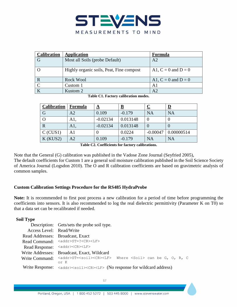
57
Calibration Application Formula
G Most all Soils (probe Default) A2
O Highly organic soils, Peat, Fine compost A1, C = 0 and D = 0
R Rock Wool A1, C = 0 and D = 0
C Custom 1 A1
K Kustom 2 A2 Table C1. Factory calibration modes.
Calibration Formula A B C D
G A2 0.109 -0.179 NA NA
O A1, -0.02134 0.013148 0 0
R A1, -0.02134 0.013148 0 0
C (CUS1) A1 0 0.0224 -0.00047 0.00000514
K (KUS2) A2 0.109 -0.179 NA NA
Table C2. Coefficients for factory calibrations.
Note that the General (G) calibration was published in the Vadose Zone Journal (Seyfried 2005),
The default coefficients for Custom 1 are a general soil moisture calibration published in the Soil Science Society
of America Journal (Logsdon 2010). The O and R calibration coefficients are based on gravimetric analysis of
common samples.
Custom Calibration Settings Procedure for the RS485 HydraProbe
Note: It is recommended to first post process a new calibration for a period of time before programming the
coefficients into sensors. It is also recommended to log the real dielectric permittivity (Parameter K on T0) so
that a data set can be recalibrated if needed.
Soil Type
Description: Gets/sets the probe soil type.
Access Level: Read/Write
Read Addresses: Broadcast, Exact
Read Command: <addr>ST=?<CR><LF>
Read Response: <addr><CR><LF>
Write Addresses: Broadcast, Exact, Wildcard
Write Command: <addr>ST=<soil><CR><LF> Where <Soil> can be G, O, R, C
or K
Write Response: <addr><soil><CR><LF> (No response for wildcard address)

58
Command Description RS485 Command
Get current calibration <addr>ST=?<CR><LF>
Switches the Probe to Custom 1 calibration <addr>ST=C<CR><LF>
Switches the Probe to Kustom 2 calibration <addr>ST=K<CR><LF>
Switches the Probe to the Organic Soil calibration <addr>ST=O<CR><LF>
Switches the Probe to the Rockwool calibration <addr>ST=R<CR><LF>
Switches the Probe to General soil calibration <addr>ST=G<CR><LF>
Sets the A coefficient <addr>XA=<value><CR><LF>
Sets the B coefficient <addr>XB=<value><CR><LF>
Sets the C coefficient <addr>XC=<value><CR><LF>
Sets the D coefficient <addr>XD=<value><CR><LF>
Verifies A coefficient <addr>XA?CR><LF> Table C3. RS485 Commands for setting soil moisture calibration. <CR> means carriage return, <LF> means line feed,
<addr> means address of probe. The default address is “000”.
The procedure below example using the commands in table C3.
Example 1(RS485)
To program a probe with an address of 000 to use the KUSTOM 2 formula, you would enter this command:
000ST=K. The KUSTOM 2 formula uses two coefficients, so we will need to assign values to them. To assign a
value of 0.3 the first coefficient and a value of -0.6 to the second, we would enter these two commands:
000XA=0.3
000XB=-0.6
To verify that your setting have been programmed into the probe, enter the following query commands. The probe
should respond as shown in boldface:
000ST=?
000K
000XA=?
000+00.30000001
000XB=?
000-00.60000002
The values that the probe returns are slightly different than the values you entered. This is an artifact of the
conversion from decimal to binary and then back again. The difference, for our purposes, is negligible.
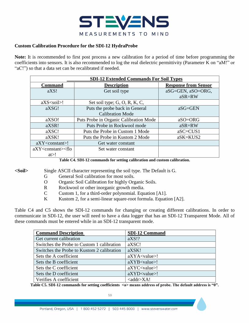
59
Custom Calibration Procedure for the SDI-12 HydraProbe
Note: It is recommended to first post process a new calibration for a period of time before programming the
coefficients into sensors. It is also recommended to log the real dielectric permittivity (Parameter K on “aM!” or
“aC!”) so that a data set can be recalibrated if needed.
SDI-12 Extended Commands For Soil Types
Command Description Response from Sensor
aXS! Get soil type aSG=GEN, aSO=ORG,
aSR=RW
aXS<soil>! Set soil type; G, O, R, K, C,
aXSG! Puts the probe back in General
Calibration Mode
aSG=GEN
aXSO! Puts Probe in Organic Calibration Mode aSO=ORG
aXSR! Puts Probe in Rockwool mode aSR=RW
aXSC! Puts the Probe in Custom 1 Mode aSC=CUS1
aXSK! Puts the Probe in Kustom 2 Mode aSK=KUS2
aXY<constant>! Get water constant
aXY<constant><flo
at>!
Set water constant
Table C4. SDI-12 commands for setting calibration and custom calibration.
<Soil> Single ASCII character representing the soil type. The Default is G.
G General Soil calibration for most soils.
O Organic Soil Calibration for highly Organic Soils.
R Rockwool or other inorganic growth media.
C Custom 1, for a third-order polynomial. Equation [A1].
K Kustom 2, for a semi-linear square-root formula. Equation [A2].
Table C4 and C5 shows the SDI-12 commands for changing or creating different calibrations. In order to
communicate in SDI-12, the user will need to have a data logger that has an SDI-12 Transparent Mode. All of
these commands must be entered while in an SDI-12 transparent mode.
Command Description SDI-12 Command
Get current calibration aXS!?
Switches the Probe to Custom 1 calibration aXSC!
Switches the Probe to Kustom 2 calibration aXSK!
Sets the A coefficient aXYA<value>!
Sets the B coefficient aXYB<value>!
Sets the C coefficient aXYC<value>!
Sets the D coefficient aXYD<value>!
Verifies A coefficient <addr>XA! Table C5. SDI-12 commands for setting coefficients <a> means address of probe. The default address is “0”.

60
Example 2. SDI-12 Procedure for custom calibration
Several commands are needed to program the HydraProbe to use a Custom Soil Setting. They are "XS" for setting
the soil type and a separate "XY" command for setting each coefficient. All commands are preceded by the probe's
address.
For example, to program a probe with an address of 0 to use the CUSTOM 1 formula, you would enter this
command:
0XSC!
0SC=CUS1
The CUSTOM 1 formula uses four coefficients, so we will need to assign the values to them. To assign a value
of -10.0 to the first coefficient, a value of 5.0 to the second, 0.3 to the third and 0.0005 to the fourth we would
enter these commands. The probes responses are shown in boldface.
0XYA-10.0!
0-10.00000000 0XYB5.0!
0+05.00000000 0XYC0.3!
0+00.30000001 0XYD0.0005!
0+00.00050000
To verify that your settings have been programmed into the probe, enter the following query commands. The
probe should respond as shown in boldface:
0XS!
0SC=CUS1
0XYA!
0-10.00000000 0XYB!
0+05.00000000 0XYC!
0+00.30000001 0XYD!
0+00.00050000
The values that the probe returns are slightly different than the values you entered. This is an artifact of the
conversion from decimal to binary and then back again. The difference, for our purposes, is negligible.
You can use the SDI-12 D commands to take current reading. For example the command
0M!
0D0!
Will return the first three reading from the first three parameters. 0D1! Will return the 2nd three readings and so
forth.

61
A Note About Scientific Notation The probe can accept values for coefficients in a form of scientific notation. The decimal number is followed by
the letter "E" and then the power of ten that is to be applied. For example:
-0.0007345 can also be entered as -7.345E-4
and
12345.678 can also be entered as 1.2345678E+4
D. Appendix - Useful links
Stevens Water Monitoring Systems, Inc.
www.stevenswater.com
The Soil Science Society of America
http://www.soils.org/
The US Department of Agriculture NRCS Soil Climate Analyses Network (SCAN)
http://www.wcc.nrcs.usda.gov/scan/
The US Department of Agriculture NRCS Snotel Network
http://www.wcc.nrcs.usda.gov/snow/
The US Bureau of Reclamation Agricultural Weather Network (AgriMet)
http://www.usbr.gov/pn/agrimet/
Free Nationwide Soil Survey Information!
https://websoilsurvey.sc.egov.usda.gov/App/HomePage.htm

62
E. Appendix - References
Blonquist, J. M., Jr., S. B. Jones, D.A. Robinson,. Standardizing Charaterization of Electromagnetic Water
Content Sensors: Part 2. Evaluation of Seven Sensing Systems. Vadose Zone J. 4:1059-1069 (2005)
Birkeland, P. W. Soils and Geomorphology 3rd Ed. Oxford University Press 1999
Campbell, J. E. 1990. Dielectric Properties and Influence of Conductivity in Soils at One to Fifty Megahertz. Soil
Sci. Soc. Am. J. 54:332-341.
Corwin, D. L., S. M. Lesch. 2003. Application of Soil Electrical Conductivity to Precision Agriculture: Theory
and Principles, and Guidelines. Agron. J. 95:455-471 (2003)
Crop and Evapotranspiration-Guidelines for Computing Crop Water Retirements Irrigation and Drainage FAO-
56, Food and Agriculture Organization of the United Nations, (1988).
Hamed, Y., M. Person, and R. Berndton. 2003. Soil Solution Electrical Conductivity Measurements Using
Different Dielectric Techniques. Soil Sci. Soc. AM. J. 67 No.4: 1071-1078
Jones, S. B., J. M. Blonquist, Jr., D.A. Robinson, V. Philip Rasmussen, and D. Or. Standardizing Charaterization
of Electromagnetic Water Content Sensors: Part 1. Methodology. Vadose Zone J. 4:1028-1058 (2005)
Lee, J. H., M. H. Oh, J. Park, S. H. Lee, K. H. Ahn, Dielectric dispersion characteristics of sand contaminated be
heavy metal, landfill leachates and BTEX (02-104) J. Hazardous Materials B105 (2003) pp. 83-102.
Logsdon, S. D., T. R. Green, M. Seyfried, S. R. Evett, and J. Bonta, Hydra Probe and Twelve-Wire Probe
Comparisons on Fluids and Cores. Soil Sci. Soc. AM. Vol. 74 No. 1, 2010.
McBride, M. B. Environmental Chemistry of Soils. Oxford University Press 1994.
Seyfried, M. S. and M. D. Murdock. 2004. Measurement of Soil Water Content with a 50-MHz Soil Dielectric
Sensor. Soil Sci. Soc. Am. J. 68:394-403.
Seyfried, M. S., L. E. Grant, = E. Du, and K. Humes. 2005. Dielectric Loss and Calibration of the HydraProbe
Soil Water Sensor. Vadose Zone Journal 4:1070-1079 (2005)
Seyfried, M.S., and L.E.Grant. 2007. Temperature Effects on soil dielectric properties measured at 50MHz.
Vadose Zone J. 6:759-765. (2007)
Topp, G. C., J. L. Davis, and A. P. Annan. 1980. Electromagnetic Determination of Soil Water Content:
Measurement in Coaxial Transmission Line. Water Resources. Res. 16:574-582
Whalley, W. R. 1993. Considerations on the use of time-domain reflectometry (TDR) for measuring soil water
content. J. Soil Sci. 44:1-9.
63
F. Appendix – CE Compliance
Declaration of Conformity
The Manufacturer of the Products covered by this Declaration is
Water Monitoring Systems, Inc.
12067 NE Glenn Widing Dr. #106
Portland, Oregon 97220 USA
503-448-8000 / 1-800-452-5272
The Directive covered by this Declaration
2004/108/EC Electromagnetic Compatibility directive
The Product Covered by this Declaration
HydraProbe soil measurement sensor
The Basis on which Conformity is being Declared
The manufacturer hereby declares that the products identified above comply with the
protection requirements of the EMC directive for and following standards to which
conformity is declared:
EN61326-1:2006
Electrical requirements for measurement, control and laboratory use EMC
requirements
Class A equipment – Conducted Emissions and Radiated Emissions
The technical documentation required to demonstrate that the products meet the requirements
of the EMC directive has been compiled and is available for inspection by the relevant
enforcement authorities.


