
ARTICLE IN PRESS
Contents lists available at ScienceDirect
Int. J. Production Economics
Int. J. Production Economics 118 (2009) 111–117
0925-52
doi:10.1
� Tel.
E-m
journal homepage: www.elsevier.com/locate/ijpe
Simultaneous determination of multiproduct batch and fulltruckload shipment schedules
Avijit Banerjee �
Department of Decision Sciences, Drexel University, Philadelphia, PA 19063, USA
a r t i c l e i n f o
Available online 20 August 2008
Keywords:
Economic lot scheduling
Full truckload shipments
Supply chain coordination
Inventory model
73/$ - see front matter & 2008 Elsevier B.V. A
016/j.ijpe.2008.08.015
: +1215 8951449; fax: +1215 895 2907.
ail address: [email protected]
a b s t r a c t
A fundamental premise of the well-known economic lot-scheduling problem (ELSP) is
that the finished products are consumed at continuous rates, i.e. their respective cycle
inventories are depleted on the basis of unit transactions. In today’s supply chains,
however, employing complex distribution networks, finished goods inventories from
manufacturing plants are usually shipped in bulk to succeeding stages along the
distribution process. Moreover, existing transport economies often tend to favor full
truckload (TL), rather that partial or less than truckload (LTL) shipments, for economical
movement of such goods. The scenario examined here, however, involves a set of
products, for which individual TL shipments are uneconomical. As a remedy, we
construct a model for taking advantage of TL rates by combining LTL quantities of the
items into a full load. We adopt the common cycle approach for the ELSP, in conjunction
with a common replenishment cycle, as a coordination mechanism that is simple to
analyze and implement. This is integrated with a periodic full truckload shipping
schedule. Such effective coordination of production and shipment schedules is likely to
result in a more streamlined supply chain. The concepts developed are illustrated
through a simple numerical example.
& 2008 Elsevier B.V. All rights reserved.
1. Introduction
The classical economic lot-scheduling problem (ELSP)involves the production of multiple products in a singlefacility or machine, which can process only one item at atime. The determination of each product’s lot size and afeasible production schedule at minimum total relevantcost are the fundamental issues of the ELSP. The ELSP hasreceived considerable research attention over the years.Past attempts to solve this problem optimally haveutilized various mathematical programming techniques,such as linear programming (Maxwell, 1964), dynamicprogramming (Bomberger, 1966; Elmaghrabi, 1978) andmixed integer programming (Delporte and Thomas, 1977).Efforts along these lines, however, have experienced
ll rights reserved.
increasing computational inefficiency as the problem sizegets larger and have concluded that the optimization ofthe ELSP becomes either inefficient or impossible for evenrelatively small problems.
Insuring the feasibility of a schedule in the ELSPappears to be a major factor of complexity, since it isNP-hard (Luenberger, 1973). The NP class of problems issolvable in nondeterministic polynomial time. There areno efficient algorithms known for this class of problems.This class of problems can be (a) solved by polynomial-time algorithms if NP is identical to P (polynomial class),or (b) proved to be permanently intractable. Therefore,most efforts in solving the ELSP during the last threedecades have been dedicated towards developing heur-istics for obtaining near-optimal solutions, rather thanoptimization (e.g. Madigan, 1968; Stankard and Gupta,1969; Doll and Whybark, 1973; Goyal, 1973; Haessler andHogue, 1976; Saipe, 1977; Elmaghrabi, 1978; Haessler,
ARTICLE IN PRESS
A. Banerjee / Int. J. Production Economics 118 (2009) 111–117112
1979; Park and Yun, 1984; Panayiotopoulos, 1983; Gengand Vickson, 1988; Davis, 1990) and by constructingfeasibility conditions (e.g. Vemuganti, 1978; Boctor,1982; Hsu, 1983; Davis, 1990).
Needless to say that within the framework of supplychain management, the ELSP has an important role to playin terms of coordinating the activities of the variousmembers of such systems. In recent years, a great deal ofresearch has focused on issues of coordinating supplyand demand within this context (see, e.g. Goyal andGupta (1989) and Thomas and Griffin (1996) for surveys).Much of the existing research on ELSP, however, assumesthat the inventory depletion rate for each of the multipleitems is uniform, which would be the case if customerdemands are satisfied directly from the manufacturingfacility. In most of today’s global firms, supply chainsconsist of complex distribution networks, involvingproduction plants, vehicle terminals, warehouses, distri-bution centers, retail outlets, etc. In such cases, thenotion of uniform product demands at a productionfacility is an incorrect representation of the real world.In reality, inventory depletions at a manufacturing plantoccur in discrete, sizeable lots, as a result of bulkshipments, that take advantage of transportation econo-mies of scale. Thus, for achieving streamlined supply chainstructures, it is necessary to link or coordinate theproduction schedule with the outbound shipment sche-dule. Unfortunately, as mentioned above, there is a dearthof research that addresses the ELSP in terms of suchlinkages.
This paper is an attempt to fill this research gap and re-examine the ELSP for developing a procedure for integrat-ing the production schedule of multiple items into ashipment plan. In other words, the primary focus here liesin coordinating the manufacturing process with thetransportation function. In shipping goods from manu-facturing facilities to subsequent stages of the supplychain, truck shipments are perhaps the most commonlyused means. Such transportation can be either fulltruckload (TL) or less than truckload (LTL) shipments.Although truck shipping rate structures are often complex,generally speaking, TL shipments are substantially lessexpensive, on a cost per unit basis, than LTL shipments(see, e.g. Chopra and Meindl, 2004). Under certaincircumstances, though, the demand rate of a productmay not be sufficiently large to warrant periodic indivi-dual TL shipments, since such large delivery lots mayresult in excessive inventory holding costs, negating theadvantage of low transportation costs. Nevertheless, ifthere is a group of such relatively low-demand productsthat are shipped from a source to various demandlocations, it may be possible to combine several partialtruckloads of individual products to constitute a fulltruckload, thus obtaining the relative advantage of TLrates, in conjunction with lower inventory levels at thedestination locations. In this study, we examine a scenariosuch as this.
In our proposed procedure for coordinating theproduction schedule of multiple products (in an ELSPenvironment) with their shipments to several demandlocations, the common production cycle approach (see,
e.g. Maxwell, 1964) is combined with the notion of adelivery (or replenishment) cycle that is common to allthe individual items. For simplicity of implementation,we restrict the production cycle to an integer multipleof the delivery cycle. Under many circumstances, asillustrated later through a numerical example andsubsequent sensitivity analysis, coordinated productionand shipment decisions, such as the one suggested inthis paper, may result in a more coherent and efficientsupply chain.
2. Assumptions and notation
2.1. Assumptions
The following assumptions, describing the manufac-turing-distribution scenario, are made in this paper:
1.
The operating environment is deterministic. 2. Multiple products are produced in a capacitated batchproduction environment, with different productionrates for the various products. We assume, withoutloss of generality, zero setup times for all the products.If, in reality, the setup times are nonzero, they can beeasily incorporated into our model, outlined later.
3.
Only a single product may be produced at any giventime.4.
Stockouts or shortages are not permitted. 5. We adopt the common cycle solution to the ELSP,where each product is produced exactly once in everyproduction cycle. Although this is a restrictiveassumption, the rationale for its adoption is threefold.First, this approach ensures a feasible solution ifsufficient capacity to produce all the products exists.Secondly, from a practitioner’s viewpoint, the com-mon cycle method is relatively easy to understandand implement, especially when stable productionand transportation schedules need to be coordinatedon a routine basis. Finally, the common cycle solu-tion can indeed be optimal or near-optimal undercertain conditions (see, Jones and Inman (1989) fordetails).
6.
Each of the products is transported via truck and soldat one or more given demand location(s). For any ofthese products, however, its market demand rate isnot sufficiently high to warrant full TL shipments. Onthe other hand, LTL shipments are relatively moreexpensive and undesirable.7.
Thus, TL shipments are made, where each truckload(capacitated by total weight and/or volume) containsa mix of all the products, which are delivered at theappropriate location(s).8.
For each TL shipment, a fixed cost is incurred,regardless of the mix of products carried. In contrast,LTL shipment rate structures often entail a unitvariable shipping cost, based on the weight and/orthe volume of shipment.9.
During each production cycle, an integer number, K, ofthese TL shipments are made at equal intervals oftime.
ARTICLE IN PRESS
A. Banerjee / Int. J. Production Economics 118 (2009) 111–117 113
10.
At each of the various demand locations, stocks arereplenished via a periodic review, order-up-to levelinventory control system. For coordination purposes,all the items at all the demand locations share acommon fixed review period.11.
The product lot sizes, Qi, are treated as continuousvariables for all i.2.2. Notation
The following notational scheme applies throughoutthis paper:
i an index used to denote a specific product, i ¼ 1,2,y, n
Di the demand rate for product i (units/time unit)Pi the production rate for product i (units/time
unit)Ai manufacturing setup cost per production batch
for product i ($/batch)hi inventory holding (carrying) cost for product i
($/unit/time unit)Qi amount of product i contained in each TL
shipment (units)K a positive integer, representing the number of
shipments per production cycle;T the shipment interval in time units (common to
all products and locations)KQi the production lot size (in units) for product i
KT production cycle length in time unitsC the TL capacity, i.e. maximum total load (or
volume) allowable per truckloadwi weight (or volume) of each unit of product i
Ii average inventory level (units) of product i
TRC total relevant cost ($) per time unit
3. Model development
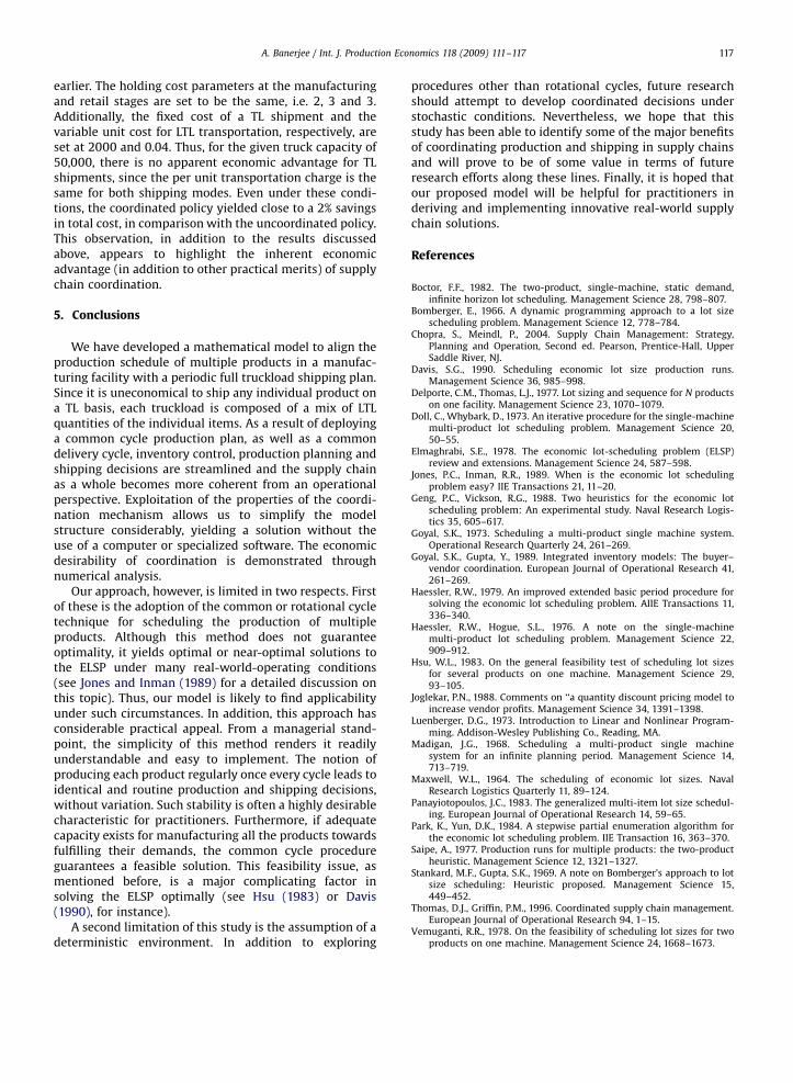
For illustrative and model development purposes, theinventory-time plots pertaining to a scenario involvingthree products (n ¼ 3) and three full TL shipments perproduction cycle (K ¼ 3), of length KT time units, aredepicted in Fig. 1.
From this figure it is clear that for a common deliverycycle time of T (i.e. T ¼ QiDi, 8i), each truckload contains Qi
units of product i, i ¼ 1, 2, 3. The total weight (or volume)in a load, w1Q1+w2Q2+w3Q3, is obviously limited to thetruck capacity, C. Also, the products should be sequencedto minimize the total inventory holding cost.
The average inventory values for the three items arecomputed as follows:
I1 ¼1
2KQ1
KQ1
P1
� �þ KQ1
KQ2
P2þ
Q3
P3
� �þ ðK � 1Þ
Q1
D1
� �Q1
�
þðK � 2ÞQ1
D1
� �Q1 þ � � � þ
Q1
D1
� �Q1
�=½KQ1=D1�
¼ KD1Q1
2P1þ
Q2
P2
� �þ D1
Q3
P3
� �þ ðK � 1Þ
Q1
2
I2 ¼1
2KQ2
KQ2
P2
� �þ KQ2
Q3
P3
� �þ ðK � 1Þ
Q2
D2
� �Q2
�
þðK � 2ÞQ2
D2
� �Q2 þ � � � þ
Q2
D2
� �Q2�=½KQ2=D2
�
¼ KD2Q2
2P2
� �þ D2
Q3
P3
� �þ ðK � 1Þ
Q2
2
I3 ¼Q3
2
D3
P3ð2� KÞ þ K � 1
� �
(for derivation see, e.g. Joglekar, 1988).In general, for the n-products case:
Ii ¼ KXn�1
i¼1
DiQi
2PiþXn�1
j¼iþ1
Qj
Pj
24
35þ Qn
Pn
Xn�1
i¼1
Di
þ ðK � 1ÞXn�1
i¼1
Qi=2; for i ¼ 1;2; . . . ;n� 1
and In ¼Qn
2
Dn
Pnð2� KÞ þ K � 1
� �
3.1. Objective function
The objective of our optimization model is to minimizethe total relevant cost per time unit, which is a function ofQ1, Q2,y, Qn (denoted by Q) and K. Thus, using the resultsobtained above, the objective function is
Minimize TRCðQ ;KÞ ¼Xn
i¼1
DiAi
KQiþ K
Xn�1
i¼1
DihiQi
2PiþXn�1
j¼iþ1
Qj
Pj
24
35
þQn
Pn
Xn�1
i¼1
Dihi þ ðK � 1ÞXn�1
i¼1
Qihi
2
þQnhn
2
Dn
Pnð2� KÞ þ K � 1
� �(1)
The first term on the RHS of (1) represents the totalsetup cost per time unit for the n products. The remainingterms, capturing the inventory holding cost per time unitfor items 1, 2,y, n�1 and n, respectively, are obtained byadding the average inventory levels, Ii, for i ¼ 1, 2,y, n�1,and In, derived above, weighted by the respective holdingcost parameters, hi and hn.
3.2. Constraints
The relevant model constraints are outlined below:
1.
The delivery cycle time is common to all products:Q1
D1¼
Q2
D2¼ � � � ¼
Qn
Dn¼ T
or Qi ¼ TDi; i ¼ 1;2; . . . ;n (2)
2.
The production capacity of the system is limited, i.e.Xn
i¼1
Di
Pip1 (3)

ARTICLE IN PRESS
P
QT
D
Q =
KQProduct 3
P
KQ
Time
KTD
KQ =
Inventory
TD
Q =
KQProduct 2
P
KQTime
KTD
KQ =
Inventory
TD
Q =
KQProduct 1
P
KQTime
KTD
KQ =
Inventory
Fig. 1. Inventory-time plots (n ¼ 3, K ¼ 3).
A. Banerjee / Int. J. Production Economics 118 (2009) 111–117114
Schedule feasibility, i.e. total production time needed
3. cannot exceed the manufacturing cycle time:KXn�1
i¼1
Qi
Piþ
Qn
PnpKT
orXn�1
i¼1
Qi
Piþ
Qn
KPnpT (4)
Note that this constraint can be easily modified fornonzero setup times by adding these to its left-hand side.
4.
Truck capacity is limited by weight or volume, i.e.Xni¼1
wiQi ¼ C (5)
3.3. Model simplification
The coordination mechanism of an equal inventoryreplenishment (or delivery) cycle time for all products
enables us to considerably simplify the non-linear mixedinteger programming problem expressed by (1)–(5).From (2)
Qi ¼ TDi; 8i or Qj ¼Q1
D1Dj; j ¼ 2;3; . . . ;n
Substituting the Qi values for all i in (5), we obtain
w1Q1 þw2Q1
D1
� �D2 þ � � � þwn
Q1
D1
� �Dn ¼ C
or Q1 ¼ CD1=Pni¼1
wiDi
and Qj ¼ TDj; j ¼ 2;3; . . . ;n:
9>>=>>; (6)
Recalling that Di for i ¼ 1,2,y, n are known parameters,T and all Qi values can be determined a priori andrecursively using (6). Now, define the parameters a, b
ARTICLE IN PRESS
A. Banerjee / Int. J. Production Economics 118 (2009) 111–117 115
and g as follows:
Pni¼1
DiAi
Qi¼ a
Pn�1
i¼1
DihiQi
2PiþPn�1
j¼iþ1
Qj
Pj
" #þPn�1
i¼1
Qihi
2þ
Qnhn
21�
Dn
Pn
� �¼ b
andQn
Pn
Pn�1
i¼1
Dihi �Pn�1
i¼1
Qihi
2þ Qnhn
Dn
Pn� 1
2
� �¼ g
9>>>>>>>>>=>>>>>>>>>;
(7)
Substituting the values Qi, i ¼ 1, 2,y, n, obtained from(6), into (7) and eliminating constraints (2) and (5), theoriginal model expressed by (1)–(5) can be considerablysimplified to
Minimize TRCðKÞ ¼ a=K þ bK þ g (8)
Subject to
Xn
i¼1
Di
Pip1; i ¼ 1;2; . . . ;n (9)
Xn�1
i¼1
Qi
Piþ
Qn
KPnpT (10)
K ¼ 1; 2; . . . ::; etc. (11)
Note that (8) is strictly convex in the integer K.Therefore, if TRC(K) is minimized at K ¼ K*, then
TRCðKnÞpTRCðKn
� 1Þ and TRCðKnÞpTRCðKn
þ 1Þ (12)
Substituting (12) into (8) we obtain the followingoptimality conditions:
KnðKn� 1Þp
abpKnðKnþ 1Þ (13)
3.4. Solution procedure
Utilizing the optimality conditions (13), the simplifiedmodel, (8)–(11), can now be easily solved by a simpleprocedure, which is outlined below:
1.
For incurring minimal inventory holding cost, se-quence the order of production by rank ordering andnumbering the n products [1], [2],y, [n] based onh½1�D½1�ph½2�D½2�p � � �ph½n�D½n�.P2.
Check constraint (9) n�1i¼1 ðDi=PiÞp1.If this constraint is violated, increase some Pi values, ifpossible, or reduce the item set, such that (9) issatisfied.
3.
Compute T, Q1 and all other Qi values using (6). 4. Calculate the parameters a and b using the definitionsin (7).
5.
Find K* from conditions (13), i.e. KnðKn� 1Þpða=bÞpKnðKnþ 1Þ. P
6.
Check constraint (10): n�1i¼1 ðQi=PiÞ þ ðQn=KPnÞpT .P7.
If violated, reset K* to Qn=ðPn½n�1i¼1 Qi=Pi � T�Þ.4. Numerical example and sensitivity analysis
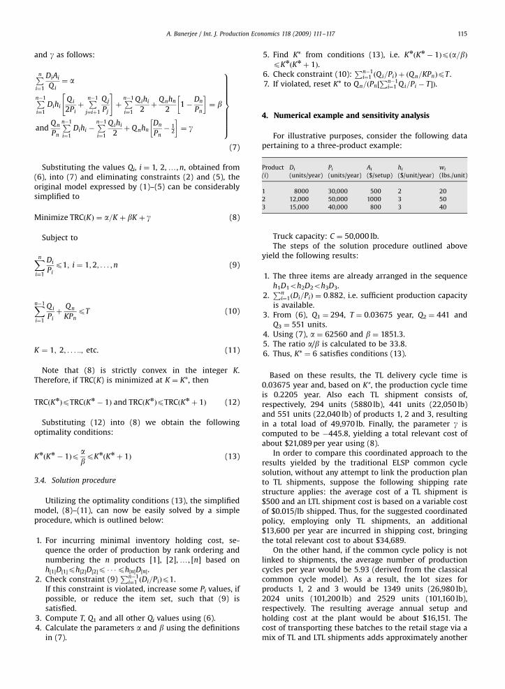
For illustrative purposes, consider the following datapertaining to a three-product example:
Product
Di Pi Ai hi wi(i)
(units/year) (units/year) ($/setup) ($/unit/year) (lbs./unit)1
8000 30,000 500 2 202
12,000 50,000 1000 3 503
15,000 40,000 800 3 40Truck capacity: C ¼ 50,000 lb.The steps of the solution procedure outlined above
yield the following results:
1.
The three items are already arranged in the sequenceh1D1oh2D2oh3D3.P2.
ni¼1ðDi=PiÞ ¼ 0:882; i.e. sufficient production capacityis available.
3. From (6), Q1 ¼ 294, T ¼ 0.03675 year, Q2 ¼ 441 andQ3 ¼ 551 units.
4. Using (7), a ¼ 62560 and b ¼ 1851.3. 5. The ratio a/b is calculated to be 33.8. 6. Thus, K* ¼ 6 satisfies conditions (13).Based on these results, the TL delivery cycle time is0.03675 year and, based on K*, the production cycle timeis 0.2205 year. Also each TL shipment consists of,respectively, 294 units (5880 lb), 441 units (22,050 lb)and 551 units (22,040 lb) of products 1, 2 and 3, resultingin a total load of 49,970 lb. Finally, the parameter g iscomputed to be �445.8, yielding a total relevant cost ofabout $21,089 per year using (8).
In order to compare this coordinated approach to theresults yielded by the traditional ELSP common cyclesolution, without any attempt to link the production planto TL shipments, suppose the following shipping ratestructure applies: the average cost of a TL shipment is$500 and an LTL shipment cost is based on a variable costof $0.015/lb shipped. Thus, for the suggested coordinatedpolicy, employing only TL shipments, an additional$13,600 per year are incurred in shipping cost, bringingthe total relevant cost to about $34,689.
On the other hand, if the common cycle policy is notlinked to shipments, the average number of productioncycles per year would be 5.93 (derived from the classicalcommon cycle model). As a result, the lot sizes forproducts 1, 2 and 3 would be 1349 units (26,980 lb),2024 units (101,200 lb) and 2529 units (101,160 lb),respectively. The resulting average annual setup andholding cost at the plant would be about $16,151. Thecost of transporting these batches to the retail stage via amix of TL and LTL shipments adds approximately another
ARTICLE IN PRESS
A. Banerjee / Int. J. Production Economics 118 (2009) 111–117116
$14,470/year. Thus, the total cost, so far, for the uncoor-dinated policy is about $30,621 a year, which is approxi-mately $4068 less per year than our suggested approach,in spite of an increase of $870 in shipping charges.However, suppose that at the retail level, the inventoryholding costs for products 1, 2 and 3 are, respectively, $3,$4 and $4 per unit per year. Now, the average annual retailinventory holding costs for the coordinated and theuncoordinated policies are, respectively, $2426 and$11,129. Therefore, from the standpoint of the entiresupply chain (production and retail facilities) the coordi-nated policy saves about $4645 (in excess of 11%) a year. Itis clear from this illustration that from a supply chainperspective, the penalties of not having coordinatedproduction and shipping schedules arise out of additionaltransportation and retail inventory holding costs.
4.1. Sensitivity analysis
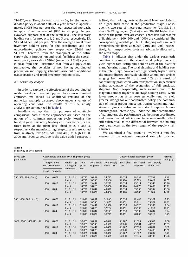
In order to explore the effectiveness of the coordinatedmodel developed here, as opposed to an uncoordinatedapproach, we solved 23 additional versions of thenumerical example discussed above under a variety ofoperating conditions. The results of this sensitivityanalysis are summarized in Table 1.
Needless to say that, for purposes of equitablecomparison, both of these approaches are based on thenotion of a common production cycle. Keeping thefinished goods inventory holding cost parameters for thethree items at the plant level fixed at 2, 3 and 3,respectively, the manufacturing setup costs sets are variedfrom relatively low (250, 500 and 400) to high (1000,2000 and 1600) values. Due to the value-added concept, it
Table 1Sensitivity analysis results
Setup cost
parameters
Coordinated common cycle shipment policy
Transportation
cost parameters
Retail-stage
holding cost
parameters
Total
plant
cost
Total re
stage co
Fixed Variable
250, 500, 400 (K ¼ 4) 300 0.009 2.1, 3.1, 3.1 14,780 10,007
3, 4, 4 14,780 10,586
500 0.015 2.1, 3.1, 3.1 14,780 15,447
3, 4, 4 14,780 16,026
1000 0.03 2.1, 3.1, 3.1 14,780 29,047
3, 4, 4 14,780 29,626
500, 1000, 800 (K ¼ 6) 300 0.009 2.1, 3.1, 3.1 21,089 10,007
3, 4, 4 21,089 10,586
500 0.015 2.1, 3.1, 3.1 21,089 15,447
3, 4, 4 21,089 16,026
1000 0.03 2.1, 3.1, 3.1 21,089 29,047
3, 4, 4 21,089 29,626
1000, 2000, 1600 (K ¼ 8) 300 0.009 2.1, 3.1, 3.1 30,005 10,007
3, 4, 4 30,005 10,586
500 0.015 2.1, 3.1, 3.1 30,005 15,447
3, 4, 4 30,005 16,026
1000 0.03 2.1, 3.1, 3.1 30,005 29,047
3, 4, 4 30,005 29,626
is likely that holding costs at the retail level are likely tobe higher than those at the production stage. Conse-quently, two sets of these parameters, i.e. (2.1, 3.1, 3.1),about 3–5% higher, and (3, 4, 4), about 30–50% higher thanthose at the plant level, are chosen. Three levels of cost fora TL shipment (300, 500 and 1000) are considered. Thecorresponding variable per lb. LTL shipping rates are keptproportionately fixed at 0.009, 0.015 and 0.03, respec-tively. All transportation costs are arbitrarily allocated tothe retail stage.
Table 1 indicates that under the various parametricconditions examined, the coordinated policy tends toyield higher total setup and holding cost at the plant ormanufacturing stage. The total shipping and holding costat the retail stage, however, are significantly higher underthe uncoordinated approach, yielding annual net savingsranging from over 6% to almost 16% as a result ofcoordinating production with transportation, in particulartaking advantage of the economies of full truckloadshipping. Not unexpectedly, such savings tend to bemagnified under higher retail stage holding costs. Whilelower production setup costs generally tend to yieldgreater savings for our coordinated policy, the combina-tion of higher production setup, transportation and retailstage carrying costs also tend to make this approach moreadvantageous. Interestingly, under the latter combinationof parameters, the performance gap between coordinatedand uncoordinated policies tend to become smaller, albeitstill substantial, as the differential between the holdingcost parameters at the two stages of the supply chainnarrows.
We examined a final scenario involving a modifiedversion of the original numerical example provided
Uncoordinated shipment policy Percent
savings (%)
tail
st
Total supply
chain cost
Total plant
cost
Total retail
stage cost
Total supply
chain cost
24,787 10,634 16,659 27,293 9.18
25,366 11,420 17,593 29,013 12.57
30,227 10,634 23,314 33,948 10.96
30,806 11,420 24,076 35,496 13.21
43,827 10,634 39,950 50,584 13.36
44,406 11,420 40,283 51,703 14.11
31,096 15,038 18,489 33,527 7.25
31,675 16,151 19,811 35,962 11.92
36,536 15,038 24,520 39,558 7.64
37,115 16,151 25,599 41,750 11.10
50,136 15,038 39,599 54,637 8.24
50,715 16,151 40,068 56,219 9.79
40,012 21,267 21,895 43,162 7.30
40,591 22,841 25,281 48,122 15.65
45,452 21,267 27,590 48,857 6.97
46,031 22,841 31,642 54,483 15.51
59,052 21,267 41,827 63,094 6.41
59,631 22,841 47,545 70,386 15.28
ARTICLE IN PRESS
A. Banerjee / Int. J. Production Economics 118 (2009) 111–117 117
earlier. The holding cost parameters at the manufacturingand retail stages are set to be the same, i.e. 2, 3 and 3.Additionally, the fixed cost of a TL shipment and thevariable unit cost for LTL transportation, respectively, areset at 2000 and 0.04. Thus, for the given truck capacity of50,000, there is no apparent economic advantage for TLshipments, since the per unit transportation charge is thesame for both shipping modes. Even under these condi-tions, the coordinated policy yielded close to a 2% savingsin total cost, in comparison with the uncoordinated policy.This observation, in addition to the results discussedabove, appears to highlight the inherent economicadvantage (in addition to other practical merits) of supplychain coordination.
5. Conclusions
We have developed a mathematical model to align theproduction schedule of multiple products in a manufac-turing facility with a periodic full truckload shipping plan.Since it is uneconomical to ship any individual product ona TL basis, each truckload is composed of a mix of LTLquantities of the individual items. As a result of deployinga common cycle production plan, as well as a commondelivery cycle, inventory control, production planning andshipping decisions are streamlined and the supply chainas a whole becomes more coherent from an operationalperspective. Exploitation of the properties of the coordi-nation mechanism allows us to simplify the modelstructure considerably, yielding a solution without theuse of a computer or specialized software. The economicdesirability of coordination is demonstrated throughnumerical analysis.
Our approach, however, is limited in two respects. Firstof these is the adoption of the common or rotational cycletechnique for scheduling the production of multipleproducts. Although this method does not guaranteeoptimality, it yields optimal or near-optimal solutions tothe ELSP under many real-world-operating conditions(see Jones and Inman (1989) for a detailed discussion onthis topic). Thus, our model is likely to find applicabilityunder such circumstances. In addition, this approach hasconsiderable practical appeal. From a managerial stand-point, the simplicity of this method renders it readilyunderstandable and easy to implement. The notion ofproducing each product regularly once every cycle leads toidentical and routine production and shipping decisions,without variation. Such stability is often a highly desirablecharacteristic for practitioners. Furthermore, if adequatecapacity exists for manufacturing all the products towardsfulfilling their demands, the common cycle procedureguarantees a feasible solution. This feasibility issue, asmentioned before, is a major complicating factor insolving the ELSP optimally (see Hsu (1983) or Davis(1990), for instance).
A second limitation of this study is the assumption of adeterministic environment. In addition to exploring
procedures other than rotational cycles, future researchshould attempt to develop coordinated decisions understochastic conditions. Nevertheless, we hope that thisstudy has been able to identify some of the major benefitsof coordinating production and shipping in supply chainsand will prove to be of some value in terms of futureresearch efforts along these lines. Finally, it is hoped thatour proposed model will be helpful for practitioners inderiving and implementing innovative real-world supplychain solutions.
References
Boctor, F.F., 1982. The two-product, single-machine, static demand,infinite horizon lot scheduling. Management Science 28, 798–807.
Bomberger, E., 1966. A dynamic programming approach to a lot sizescheduling problem. Management Science 12, 778–784.
Chopra, S., Meindl, P., 2004. Supply Chain Management: Strategy,Planning and Operation, Second ed. Pearson, Prentice-Hall, UpperSaddle River, NJ.
Davis, S.G., 1990. Scheduling economic lot size production runs.Management Science 36, 985–998.
Delporte, C.M., Thomas, L.J., 1977. Lot sizing and sequence for N productson one facility. Management Science 23, 1070–1079.
Doll, C., Whybark, D., 1973. An iterative procedure for the single-machinemulti-product lot scheduling problem. Management Science 20,50–55.
Elmaghrabi, S.E., 1978. The economic lot-scheduling problem (ELSP)review and extensions. Management Science 24, 587–598.
Jones, P.C., Inman, R.R., 1989. When is the economic lot schedulingproblem easy? IIE Transactions 21, 11–20.
Geng, P.C., Vickson, R.G., 1988. Two heuristics for the economic lotscheduling problem: An experimental study. Naval Research Logis-tics 35, 605–617.
Goyal, S.K., 1973. Scheduling a multi-product single machine system.Operational Research Quarterly 24, 261–269.
Goyal, S.K., Gupta, Y., 1989. Integrated inventory models: The buyer–vendor coordination. European Journal of Operational Research 41,261–269.
Haessler, R.W., 1979. An improved extended basic period procedure forsolving the economic lot scheduling problem. AIIE Transactions 11,336–340.
Haessler, R.W., Hogue, S.L., 1976. A note on the single-machinemulti-product lot scheduling problem. Management Science 22,909–912.
Hsu, W.L., 1983. On the general feasibility test of scheduling lot sizesfor several products on one machine. Management Science 29,93–105.
Joglekar, P.N., 1988. Comments on ‘‘a quantity discount pricing model toincrease vendor profits. Management Science 34, 1391–1398.
Luenberger, D.G., 1973. Introduction to Linear and Nonlinear Program-ming. Addison-Wesley Publishing Co., Reading, MA.
Madigan, J.G., 1968. Scheduling a multi-product single machinesystem for an infinite planning period. Management Science 14,713–719.
Maxwell, W.L., 1964. The scheduling of economic lot sizes. NavalResearch Logistics Quarterly 11, 89–124.
Panayiotopoulos, J.C., 1983. The generalized multi-item lot size schedul-ing. European Journal of Operational Research 14, 59–65.
Park, K., Yun, D.K., 1984. A stepwise partial enumeration algorithm forthe economic lot scheduling problem. IIE Transaction 16, 363–370.
Saipe, A., 1977. Production runs for multiple products: the two-productheuristic. Management Science 12, 1321–1327.
Stankard, M.F., Gupta, S.K., 1969. A note on Bomberger’s approach to lotsize scheduling: Heuristic proposed. Management Science 15,449–452.
Thomas, D.J., Griffin, P.M., 1996. Coordinated supply chain management.European Journal of Operational Research 94, 1–15.
Vemuganti, R.R., 1978. On the feasibility of scheduling lot sizes for twoproducts on one machine. Management Science 24, 1668–1673.


