
Part IA Engineering
Mathematics
Lent Term
Convolution
Fourier Series
Probability
Richard PragerJanuary 2012
1
Contents & Examples Questions
Section 1 Linear System & Impulse ResponsePaper 7: questions 1–3.
Section 2 Differential Equations to DescribeLinear SystemsPaper 7: questions 4 and 5.
Section 3 ConvolutionPaper 7: questions 6 and 7.
Section 4 Evaluating Convolution IntegralsPaper 7: question 8.
Section 5 Fourier SeriesPaper 8: questions 1 and 2.
2
Contents & Examples Qs contd.
Section 6 General Fourier SeriesPaper 8: question 3 and first part of 4.
Section 7 Convergence & Half Range SeriesesPaper 8: end of Q4 and questions 5–7
Section 8 Complex Fourier SeriesPaper 8: question 8.
Section 9 ProbabilityPaper 9: questions 1–12,
Section 10 StatisticsPaper 9: questions 13 and 14.
3
Section 1
Linear System & Impulse Response
We motivate the study of linear time-invariant systems.
The principle of superposition is explained.
Step functions and delta functions are introduced, to-gether with their corresponding responses.
Examples are given to illustrate the use of the stepresponse with superposition.
The sifting theorem is stated and illustrated with someexamples.
4

Motivation
Many engineering problems concern linear systems.
System
System
System
System
System
Forces Strains
Voltages Currents
DensityPressure
Temperature
Power
Heat flow
Kinetic Energy
In a linear system the output is computed as somelinear combination of the inputs (including inputs fromthe past, if we are considering a system with a time-varying input and output).
5
Linear Systems
LinearSystem
f(t) y(t)
1. Linear time-invariant systems satisfy the principleof superposition.
If input f1(t) → output y1(t)and input f2(t) → output y2(t)
theninput αf1(t) + βf2(t) → output αy1(t) + βy2(t)where α and β are any constants.
2. Linear systems have the special property that asine wave at the input leads to a (possibly different)sine wave at the output.
Sine wave withamplitude orLinear
SystemSine wave
phase changed
6

Step Function
H(t)
t
H(t) =
{
0, t < 01, t > 0
LinearSystem step response
H(t) r(t)
7
Superposition Example
H(t) r(t)
1 1
H(t−1) r(t−1)
−H(t−1) −r(t−1)
LinearSystem
H(t) − H(t−1)
1 1
r(t) − r(t−1)
8

Calculation of Superposition
1
f(t)
t
2
Find the output of a linear systemwith step response
r(t) =
{
0, t < 0
1− e−5t, t ≥ 0
when the input is the pulse f(t).
Case (a): When 0 ≤ t < 1 the input is the same as ascaled step function so the output y(t) is given by
y(t) = 2(
1− e−5t)
,0 ≤ t < 1
Case (b): When 1 ≤ t
f(t) = 2H(t)− 2H(t− 1)
therefore the output y(t) is given by
y(t) = 2r(t)− 2r(t− 1)
= 2(
1− e−5t − 1+ e−5(t−1))
= 2(
e5 − 1)
e−5t ,1 ≤ t
9
Dirac Delta Function
tw/2−w/2
f(t)height = 1/w
As w → 0 the pulse f(t) becomes narrower andtaller. In the limit as w → 0 the pulse f(t) becomes adelta function: δ(t).
The delta function is a spike with unit area. It goesbang when its argument is zero.
δ(t) = 0 except at t = 0∫ b
aδ(t)dt = 1 provided a < 0 and b > 0
LinearSystem
δ(t) impulse response
10
Integrating the Delta Function
From the previous page∫ b
aδ(t) dt = 1 provided a < 0 and b > 0
thus∫ T
−∞δ(t) dt =
{
0, T < 01, T > 0
= H(T)
The integral of a delta function is a step function.
Conversely, the derivative of a step function is a deltafunction.
δ
DeltaFunction (t)
StepFunctionH(t)differentiate
integrate
11
Impulse Response
ImpulseResponseg(t)
Step
differentiate
integrateResponser(t)
Find the output, g(t) of a linear system with step re-sponse r(t) = 1 − e−5t when the input is the deltafunction δ(t).
r(t) = 1− e−5t
g(t) =dr
dt= 5e−5t
So the impulse response of the system is 5e−5t.
12

Sifting Theorem
tb
f(t)
δ(t−b)
a b c t
f(t)
δ(t−b)
a b c t
∫ c
aδ(t− b)dt = 1 provided a < b and c > b
∫ c
aδ(t− b)f(t)dt = f(b) provided a < b and c > b
13
Sifting Examples
∫ π
−πcos(2t) δ(t) dt = cos(0) = 1
∫ π
−πcos(2t) δ
(
t− π
2
)
dt = cos(π) = −1
∫ 0
−πcos(2t) δ
(
t− π
2
)
dt = 0
∫ π
−πt δ
(
t+π
2
)
dt = −π
2∫ π
0t δ
(
t+π
2
)
dt = 0
14

Section 1: Summary
Superposition:If input f1(t) → output y1(t)and input f2(t) → output y2(t) theninput αf1(t) + βf2(t) → output αy1(t) + βy2(t)where α and β are any constants.
Sifting:∫ c
aδ(t− b)f(t)dt = f(b) provided a < b and c > b
Step function and step response.
Impulse function and impulse response.
Finding the system response to a pulse by combiningscaled and delayed step responses using superposi-tion.
15
Section 2
Differential Equations to
Describe Linear Systems
We motivate the convolution integral, which will bepresented in section 3, using an example of a car go-ing up a step.
A technique is described for solving a linear differen-tial equation to obtain the step response of the sys-tem. We set the input to 1, and solve with initial con-ditions y = y = 0 for t = 0. The impulse responsecan then be obtained by differentiating the step re-sponse.
The utility of this technique, when used together withconvolution, is outlined.
16

Differential Equations
Linear systems are often described using differentialequations. For example:
d2y
dt2+5
dy
dt+6y = f(t)
where f(t) is the input to the system and y(t) is theoutput.
We know how to solve for y given a specific input f .
We now cover an alternative approach:
EquationDifferential
convolution Corresponding Output
solve
Any input
Impulse response
17
Solving for Impulse Response
We cannot solve for the impulse response directly sowe solve for the step response and then differentiate
it to get the impulse response.
convolution Corresponding Output
EquationDifferential solve
differentiate
Any input
Impulse response
Step response
18

Motivation: Convolution
If we know the response of a linear system to a stepinput, we can calculate the impulse response and hencewe can find the response to any input by convolution.
Suppose we want to know how a car’s suspension re-sponds to lots of different types of road surface.
We measure how the suspension responds to a stepinput (or calculate the step response from a theoreti-cal model of the system).
We can then find the impulse response and use con-volution to find the car’s behaviour for any road sur-face profile.
19
Solving for Step Response
If we want to find the step response of
dy
dt+5y = f(t)
where f is the input and y is the output. It would benice if we could put f(t) = H(t) and solve. Unfortu-nately we don’t know of a way to do this directly. So
we
1. set f(t) = 1, and solve for just t ≥ 0
2. set the boundary condition y(0) = 0 (also y(0) =
0 for second order equations) to imply that f(t)was zero for all t < 0.
We thus have a complete solution because y = 0 fort < 0, and we have found y for all t ≥ 0.
20

Boundary Condition Justification
Prove that y = 0 at t = 0 by contradiction.
We know that y(t) = 0 for all t < 0. Therefore theonly way for y to equal something other than zero att = 0 is if there is a step discontinuity in y at t = 0 .
Assume that y has a step of height h at t = 0 . If y
has a step discontinuity at t = 0 then dydt must have
a delta function at t = 0.
So we have:
• f(t) is a step function so |f(t)| ≤ 1 for all t.
• |y| ≤ h at t = 0.
•∣
∣
∣
dydt
∣
∣
∣ → ∞ at t = 0.
Which violates the original equation at t = 0.
dy
dt= f(t)− 5y
As the RHS is finite but the LHS is infinite. Thereforey must be continuous at t = 0, and we can use theinitial condition y(0) = 0.
21
Step Response Example
Step 1: set f(t) = 1, and solve for just t ≥ 0.
dy
dt+5y = 1
Complimentary function: y +5y = 0 ⇒ y = Ae−5t
Particular Integral: try y = λ (a const) ⇒ y = 15
General Solution: y = Ae−5t + 15
Step 2: set the boundary condition y = 0 at t = 0
y(0) = 0 ⇒ A+ 15 = 0 ⇒ A = −1
5
So step response is y(t) = 15
(
1− e−5t)
for t ≥ 0.
22

Step → Impulse Response
ImpulseResponseg(t)
Step
differentiate
integrateResponse
Step response is y(t) = 15
(
1− e−5t)
for t ≥ 0.
Impulse response g(t) is given by:
g(t) =
0, t < 0
d
dt
[
1
5
(
1− e−5t)
]
= e−5t, t ≥ 0
23
Find the Impulse Response
d2y
dt2+13
dy
dt+12y = f(t)
1. Find the General Solution with f(t) = 1
Complimentary function is y = Ae−12t +Be−t
Particular integral is y = 112
General solution is y = 112 +Ae−12t +Be−t
2. Set boundary conditions y(0) = y(0) = 0 to getthe step response.
112 +A+B = 0
−12A−B = 0
⇒ A = 1132 and B = − 1
11
Thus Step Response is y = 112 + e−12t
132 − e−t
11
3. Differentiate the step response to get the impulseresponse.
g(t) =dy
dt=
e−t − e−12t
11, (t ≥ 0)
24

Using the Impulse Response
If we have a system input composed of impulses,
f(t) = 3δ(t− 1) + 4δ(t− 2)
we can find the corresponding system output usingsuperposition.
For t ≥ 2
y(t) = 3g(t− 1) + 4g(t− 2)
= 3
e−(t−1) − e−12(t−1)
11
+4
e−(t−2) − e−12(t−2)
11
25
More General Input
Suppose our input is composed of lots of delta func-tions:
f(t) =∑
npn δ(t− qn)
Then the corresponding system output will be
y(t) =∑
npn g(t− qn)
26

Section 2: Summary
ay + by + cy + d = f(t)Differential Equation
convolution Corresponding Output
differentiate
ay + by + cy + d = 1
Any input
Impulse response
Step response
solve
with boundary conditions y(0) = 0 and y(0) = 0
27
Section 3
Convolution
In this section we derive the convolution integral andshow its use in some examples.
28

Convolution
Our goal is to calculate the output, y(t) of a linear sys-tem using the input, f(t), and the impulse responseof the system, g(t).
An impulse at time t = 0 produces the impulse re-sponse.
LinearSystem
t t
(t)δ g(t)
An impulse delayed to time t = τ produces a delayedimpulse response starting at time τ .
LinearSystem
g(t− )τ
τ τt t
τ(t− )δ
29
A scaled impulse at time t = 0 produces a scaledimpulse response.
LinearSystem
t t
g(t)δ(t)k k
An impulse that has been scaled by k and delayed totime t = τ produces an impulse response scaled byk and starting at time τ .
LinearSystem
g(t− )τ
τ τt t
τ(t− )δk k
30
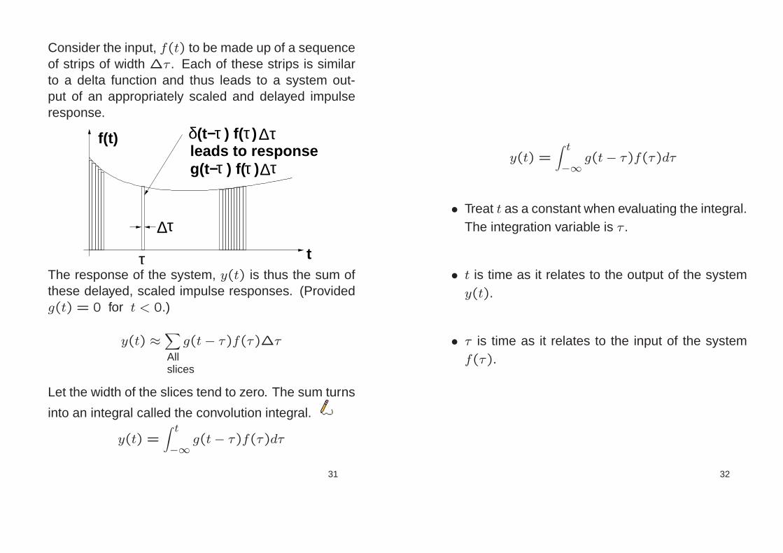
Consider the input, f(t) to be made up of a sequenceof strips of width ∆τ . Each of these strips is similarto a delta function and thus leads to a system out-put of an appropriately scaled and delayed impulseresponse.
(t− ) f( )δ τ τ ∆τ
∆τ
∆τ
τ t
f(t)leads to responseg(t− ) f( )τ τ
The response of the system, y(t) is thus the sum ofthese delayed, scaled impulse responses. (Providedg(t) = 0 for t < 0.)
y(t) ≈∑
Allslices
g(t− τ)f(τ)∆τ
Let the width of the slices tend to zero. The sum turns
into an integral called the convolution integral.
y(t) =
∫ t
−∞g(t− τ)f(τ)dτ
31
y(t) =∫ t
−∞g(t− τ)f(τ)dτ
• Treat t as a constant when evaluating the integral.The integration variable is τ .
• t is time as it relates to the output of the systemy(t).
• τ is time as it relates to the input of the systemf(τ).
32

Convolution Example 1
Consider a system with impulse response
g(t) =
{
0 , t < 0
e−5t , t ≥ 0
Find the output for input f(t) = H(t) (step function).
y(t) =
∫ t
−∞g(t− τ)f(τ)dτ
=∫ t
−∞e−5(t−τ)H(τ)dτ
=
∫ t
0e−5(t−τ)dτ
=
[
1
5e−5(t−τ)
]t
0
=1
5
(
1− e−5t)
33
Convolution Example 2
For the same system (g(t) = e−5t, t ≥ 0), find theoutput for input
f(t) =
0, t < 0v, 0 < t < k0, t > k
k
vf(t)
t
Using the convolution integral, the answer is given by
y(t) =∫ t
−∞g(t− τ)f(τ)dτ
=
∫ t−∞ g(t− τ)× 0 dτ, t < 0
∫ 0−∞ g(t− τ)× 0 dτ
+∫ t0 g(t− τ) v dτ, 0 < t < k
∫ 0−∞ g(t− τ)× 0 dτ
+∫ k0 g(t− τ) v dτ
+∫ tk g(t− τ)× 0 dτ, t > k
34

Case (a): t < 0
∫ t−∞ g(t− τ)× 0 dτ = 0 so y(t) = 0 for all t < 0.
Case (b): 0 < t < k
y(t) =
∫ t
0g(t− τ) v dτ =
∫ t
0e−5(t−τ) v dτ
=v
5
[
e−5(t−τ)]t
0
=v
5
(
1− e−5t)
Case (c): t > k
y(t) =
∫ k
0g(t− τ) v dτ =
∫ k
0e−5(t−τ) v dτ
=v
5
[
e−5(t−τ)]k
0
=v
5
(
e5k − 1)
e−5t
(a) (b) (c)k
y(t)
t
35
Convolution Example 3
For the same system (g(t) = e−5t, t ≥ 0), find theoutput for input
f(t) =
{
0, t < 0sin(ωt), t > 0
t
f(t)
Using the convolution integral, the answer is given by
y(t) =
∫ t
−∞g(t− τ)f(τ)dτ
=
∫ t−∞ g(t− τ)× 0 dτ, t < 0
∫ 0−∞ g(t− τ)× 0 dτ
+∫ t0 g(t− τ) sin(ωτ) dτ, 0 < t
36
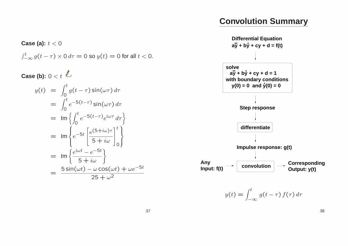
Case (a): t < 0
∫ t−∞ g(t− τ)× 0 dτ = 0 so y(t) = 0 for all t < 0.
Case (b): 0 < t
y(t) =
∫ t
0g(t− τ) sin(ωτ) dτ
=∫ t
0e−5(t−τ) sin(ωτ) dτ
= Im{∫ t
0e−5(t−τ)eiωτ dτ
}
= Im
e−5t
e(5+iω)τ
5 + iω
t
0
= Im
{
eiωt − e−5t
5+ iω
}
=5sin(ωt)− ω cos(ωt) + ωe−5t
25 + ω2
37
Convolution Summary
ay + by + cy + d = f(t)Differential Equation
convolution
differentiate
ay + by + cy + d = 1
Step response
solve
with boundary conditions y(0) = 0 and y(0) = 0
Corresponding
Impulse response: g(t)
Output: y(t)AnyInput: f(t)
y(t) =
∫ t
−∞g(t− τ) f(τ) dτ
38

Complete Example
Find the impulse response of
d2y
dt2+3
dy
dt+2y = f(t)
hence find the output when the input f(t) = H(t)e−t.
1. Find the General Solution with f(t) = 1
Complimentary function is y = Ae−t +Be−2t
Particular integral is y = 12
General solution is y = 12 +Ae−t +Be−2t
2. Set boundary conditions y(0) = y(0) = 0 to getthe step response.
12 +A+B = 0
−A− 2B = 0
⇒ A = −1 and B = 12
Thus Step Response is y = 12 − e−t + e−2t
2
39
3. Differentiate the step response to get the impulseresponse.
g(t) =dy
dt= e−t − e−2t
4. Use the convolution integral to find the output forthe required input.
The required input is f(t) = e−t , t > 0.
y(t) =
∫ t
−∞g(t− τ)f(τ)dτ
=
∫ t
0
(
e−(t−τ) − e−2(t−τ))
e−τ dτ
=
∫ t
0e−t − eτ−2t dτ
=[
τe−t − eτ−2t]t
0
= (t− 1) e−t + e−2t
40

Section 3: Summary
Convolution integral (memorise this):
f(t) = input
g(t) = impulse response
y(t) = output
y(t) =∫ t
−∞g(t− τ) f(τ) dτ
Way to find the output of a linear system, describedby a differential equation, for an arbitrary input:
• Find general solution to equation for input = 1.
• Set boundary conditions y(0) = y(0) = 0 to getthe step response.
• Differentiate to get the impulse response.
• Use convolution integral together with the impulseresponse to find the output for any desired input.
41
Section 4
Evaluating Convolution Integrals
A way of rearranging the convolution integral is de-scribed and illustrated.
The differences between convolution in time and spaceare discussed and the concept of causality is intro-duced.
The concept of a spatially-varying impulse is intro-duced and the section ends with an example of spatialconvolution with a spatially-varying impulse response.
42

Convolution Summary
ay + by + cy + d = f(t)Differential Equation
convolution
differentiate
ay + by + cy + d = 1
Step response
solve
with boundary conditions y(0) = 0 and y(0) = 0
Corresponding
Impulse response: g(t)
Output: y(t)AnyInput: f(t)
y(t) =
∫ t
−∞g(t− τ) f(τ) dτ
43
Splitting up Integrals
Suppose we have a function:
f(t) =
a , t < 0b , 0 < t < kc , k < t
and we want to evaluate the integral∫ t−∞ f(τ) dτ , we
can split it up as follows:
∫ t−∞ a dτ , t < 0
∫ 0−∞ a dτ +
∫ t0 b dτ , 0 < t < k
∫ 0−∞ a dτ +
∫ k0 b dτ +
∫ tk c dτ , k < t
44

ExampleFind the impulse response of
d2y
dt2+9y = f(t)
hence find the output for (i) input f(t) = t, t > 0 and(ii) input f(t) = H(t)−H(t− 1).
1. Find the General Solution with f(t) = 1
Complimentary function is y = A cos(3t)+B sin(3t)
Particular integral is y = 19
General solution is y = 19 +A cos(3t) +B sin(3t)
2. Set boundary conditions y(0) = y(0) = 0 to getthe step response.
19 +A = 0
3B = 0
⇒ A = −19 and B = 0
Thus the Step Response is
y =1
9(1− cos(3t))
45
3. Differentiate the step response to get the impulseresponse.
g(t) =dy
dt=
1
3sin(3t)
4. Use the convolution integral to find the output forthe required input.
For part (i) the required input is a ramp starting at theorigin: f(t) = t when t > 0 and f(t) = 0 otherwise.
y(t) =∫ t
−∞g(t− τ)f(τ) dτ
=∫ t
0
1
3sin(3(t− τ))× τ dτ
=t
9− sin(3t)
27
0 1 2 3 4 50
0.2
0.4
0.6
t
y(t)
46

For part (ii) the required input is a pulse of unit heightand unit duration: f(t) = H(t)−H(t− 1).
y(t) =
∫ t
−∞g(t− τ)f(τ)dτ
=
∫ t−∞ g(t− τ)× 0 dτ, t < 0
∫ 0−∞ g(t− τ)× 0 dτ
+∫ t0 g(t− τ)× 1 dτ, 0 < t < 1
∫ 0−∞ g(t− τ)× 0 dτ
+∫ 10 g(t− τ)× 1 dτ
+∫ t1 g(t− τ)× 0 dτ, t > 1
47
Case (a): t < 0
∫ t−∞ g(t− τ)× 0 dτ = 0 so y(t) = 0 for all t < 0.
Case (b): 0 < t < 1
y(t) =
∫ t
0g(t− τ)× 1 dτ =
∫ t
0
1
3sin(3(t− τ)) dτ
=1
9(1− cos(3t))
Case (c): 1 < t
y(t) =
∫ 1
0g(t− τ)× 1 dτ =
∫ 1
0
1
3sin(3(t− τ)) dτ
=
[
1
9cos(3(t− τ))
]1
0
=1
9{cos(3(t− 1))− cos(3t)}
48

Part (ii) Another Way
The input for part (ii) is composed of two step func-tions. We can therefore calculate the output using thestep response, r(t) = 1
9(1− cos(3t)).
Input = H(t)−H(t−1) ⇒ Output = r(t)−r(t−1)
Hence, for t > 1,
y(t) =1
9(1− cos(3t))− 1
9(1− cos(3(t− 1)))
=1
9{cos(3(t− 1))− cos(3t)}
49
Alternate Convolution Integral
The normal convolution integral
y(t) =
∫ t
−∞g(t− τ) f(τ) dτ
can be inconvenient to compute when we have a com-plicated expression for g(t).
We would therefore like to derive an alternative ver-sion of the convolution integral that has a term of theform g(τ) rather than g(t− τ) as this will be easierto calculate in cases where g is a complicated expres-sion.
50

Arguments of f and g
Substitute u = t − τ in the convolution formula. As-sume all signals are zero for t < 0 and set the lowerintegral limit to zero. We have −du = dτ ,∫ t
0g(t− τ)f(τ)dτ = −
∫ 0
tg(u)f(t− u)du
=
∫ t
0g(u)f(t− u)du
As u is the variable of integration, we can call it any-thing, as it disappears when the integration has beenevaluated. We therefore choose to rename u as τ .Hence:
∫ t
0g(t− τ)f(τ)dτ =
∫ t
0g(τ)f(t− τ)dτ
So it does not matter which way round you get the ar-guments to the functions in the convolutions integral,provided both functions are zero for t < 0.
51
Example
Consider a linear system with impulse response
g(t) =
{
3t2 − 4t+7 , t > 00 , otherwise
Find the output for the input f(t) = t, (t ≥ 0) andf(t) = 0, (t < 0).
Note that everything is zero for t < 0, so we can usey(t) =
∫ t0 f(t− τ)g(τ) dτ .
y(t) =
∫ t
0f(t− τ)g(τ) dτ
=∫ t
0(t− τ)× (3τ2 − 4τ +7) dτ
=t4
4− 2t3
3+
7t2
2
52

Spatial Convolution
Systems with time-varying input & output.
Causal: no output before the input that causes it.g(t) = 0, t < 0
Systems with input, output a function of position.
An input can affect the output on either side. g(x) canbe non-zero for any x.
Consider a one-dimensional strip of a material that isknown to deform linearly according to
g(x) =1
cosh(x)x
g(x)
when subject to a unit force at x = 0.
This is a spatial impulse response.
53
Spatial Convolution Example
x
f(x)
0 2
1
Calculate the deformation of a stripof material with spatial impulse re-sponse as described on the previ-ous page in response to a uniformload of f(x) = 1.0 applied from x = 0 to x = 2.
y(x) =
∫ ∞
−∞g(x− τ)f(τ) dτ
=
∫ 0
−∞1
cosh(x− τ)× 0 dτ
+
∫ 2
0
1
cosh(x− τ)× 1 dτ
+∫ ∞
2
1
cosh(x− τ)× 0 dτ
=∫ 2
0
1
cosh(x− τ)dτ
= 2{
arctan(
e2−x)
− arctan(
e−x)}
54
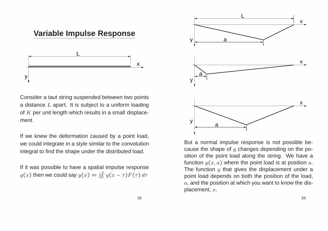
Variable Impulse Response
x
L
y
Consider a taut string suspended between two pointsa distance L apart. It is subject to a uniform loadingof K per unit length which results in a small displace-ment.
If we knew the deformation caused by a point load,we could integrate in a style similar to the convolutionintegral to find the shape under the distributed load.
If it was possible to have a spatial impulse responseg(x) then we could say y(x) =
∫L0 g(x− τ)F(τ) dτ
55
xL
y
x
y
x
ya
a
a
But a normal impulse response is not possible be-cause the shape of g changes depending on the po-sition of the point load along the string. We have afunction g(x, a) where the point load is at position a.The function g that gives the displacement under apoint load depends on both the position of the load,a, and the position at which you want to know the dis-placement, x.
56

If we can find this g(x, a) we can work out the com-plete displacement under the continuous load K us-ing
y(x) =
∫ L
0g(x, a)F(a) da =
∫ L
0g(x, a)K da
F
a
y
T T
1r 2r
21
Segment 1 Segment 2
d
x
L
To find g(x, a) we first work out the maximum dis-placement, d, for a point load, F = 1, at positiona.
Resolve horisontally: T1 cos(r1) = T2 cos(r2)
Use the approximation: cos(r1) ≈ cos(r2) ≈ 1
This gives us: T1 = T2. Call this tension T .
57
Now resolve vertically: T(sin(r1) + sin(r2)) = 1
Again approximate: cos(r1) ≈ cos(r2) ≈ 1
This gives us: T(tan(r1) + tan(r2)) = 1
⇒(
d
a+
d
L− a
)
=1
T
⇒ Ld
a(L− a)=
1
T
so d =a(L− a)
TL
This enables us to write down equations for the twostraight segments of the g(x, a) function.
Segment 1:x < a
g(x, a) =
(
x
a
)
d =x(L− a)
TL
Segment 2:x > a
g(x, a) =
(
L− x
L− a
)
d =a(L− x)
TL
58

Finally, we work out the shape of a string of lengthL with tension T under a uniform load of K per unitlength.
y(x) =
∫ L
0g(x, a)F(a) da
=
∫ L
0g(x, a)K da
=
∫ x
0g
seg 2 ×K da+
∫ L
xg
seg 1 ×K da
=∫ x
0
a(L− x)K
TLda+
∫ L
x
x(L− a)K
TLda
=
(
K
2T
)
x(L− x)
59
Section 4: Summary
If f(t) = g(t) = 0 for all t < 0 then
∫ t
0g(t− τ)f(τ)dτ =
∫ t
0g(τ)f(t− τ)dτ
Systems for which g(t) = 0 for all t < 0 are calledcausal systems.
Systems with time-varying inputs and outputs are causal.
Systems that have inputs and outputs that vary as afunction of spatial location can have g(x) 6= 0 for anyx.
We have learnt how to handle a spatially-varying im-pulse response.
60

Section 5
Fourier Series
The Fourier series is introduced using an analogy withsplitting vectors up into components.
The symmetry properties that enable us to predict thatcertain coefficients are zero are presented.
61
Motivation
We mentioned at the start of the last section that sinewaves have a special property in relation to linear sys-tems.
Sine wave withamplitude orLinear
SystemSine wave
phase changed
A sine wave at the inputleads to a (possibly differ-ent) sine wave at the out-put.
It would therefore be useful to be able to express anarbitrary signal in terms of a sum of sine waves.
originalsignal
split intosine waves
System output
recombine
62

Motivation: Car Suspension
Supposing we know that our car suspension will startto oscillate (bounce up and down uncomfortably) atfrequency f .
We want to measure a variety of typical road profilesand calculate how much of frequency f they eachcontain (with the car travelling at a particular speed).
This will tell us which combinations of road profile andspeed are likely to be a problem.
The Fourier series enables us to represent the roadprofile as the sum of a set of sinusoidal componentsat different frequencies.
63
Splitting up Vectors
We want to express a signal f(t) in the range −π ≤t ≤ π in terms of some basic signals, i.e. sine waves.Let’s look first at how we do a similar thing with vec-tors.
Consider how we express the arbitrary vector r in termsof the basis vectors i and j.
j
i
a = r . ii i.
b = r . j
j j.
where
r = a i + b j
The basis vectors are orthogonal: i.j = 0.
64

Basis Functions
Just as we represent r using orthogonal basis vectors,we want to represent f(t) in the range −π to π usingorthogonal basis functions. We only need two vectors,but we need an infinite number of functions.
1 (i.e. a constant term)cos(t) cos(2t) cos(3t) cos(4t) . . .sin(t) sin(2t) sin(3t) sin(4t) . . .
If n and m are positive integers greater than zero.∫ π−π cos(nt) sin(mt) dt = 0
∫ π−π cos(nt)× 1 dt = 0∫ π−π sin(nt)× 1 dt = 0
∫ π
−πcos(nt) cos(mt) dt =
{
0 , n 6= mπ , n = m
∫ π
−πsin(nt) sin(mt) dt =
{
0 , n 6= mπ , n = m
∫ π
−π1× 1 dt = 2π
So, using∫ π−π p(t)q(t) dt as our “dot product for func-
tions”, the basis functions are orthogonal.
65
Fourier Series
The equivalents of our vector dot product expressionsto calculate the component of r in each direction (eg.a = (r.i)/(i.i)) are:
an =
∫ π−π cos(nt)f(t) dt
∫ π−π cos(nt) cos(nt) dt
=1
π
∫ π
−πcos(nt)f(t) dt
bn =
∫ π−π sin(nt)f(t) dt
∫ π−π sin(nt) sin(nt) dt
=1
π
∫ π
−πsin(nt)f(t) dt
d =
∫ π−π 1×f(t) dt∫ π−π 1×1 dt
=1
2π
∫ π
−πf(t) dt
The equivalent of our vector expression for r in termsof i and j, (i.e. r = ai + bj) is an expression for f in
terms of all the basis functions.
f(t) =∞∑
n=1
an cos(nt) +∞∑
n=1
bn sin(nt) + d× 1
66

Fourier Series Example 1
−π π
1−1
f(t)
t2π−2π
Represent the square wavef(t) as a Fourier series.
an =1
π
∫ π
−πcos(nt)f(t) dt = 0
bn =1
π
∫ π
−πsin(nt)f(t) dt =
2(1− (−1)n)
nπ
d =1
2π
∫ π
−πf(t) dt = 0
Thus, we can model the square wave function f(t)
using:
f(t) = d+∞∑
n=1
(an cos(nt) + bn sin(nt))
=∞∑
n=1
2 (1− (−1)n)
nπsin(nt)
=4
π
[
sin(t) +sin(3t)
3+
sin(5t)
5+ . . .
]
67
Fourier Series Properties
1. We can use any range of length 2π instead of−π ≤ t ≤ π in the Fourier formulae. For example,0 ≤ t ≤ 2π is equally OK.
2. We are only modelling the function f(t) in thespecified range (eg. −π to π, or 0 to 2π). Outsidethis range the model will just repeat with period 2π.
This is fine if the function we wish to model is peri-odic itself, but if the function is not periodic the Fouriermodel will probably only be useful over the range onwhich it was built.
2π
Fourier series representationbased on range 0 to 2 π
Original function
0
68

Fourier Series Example 2
Represent f(t) = et as a Fourier series between −π
and π.
an =1
π
∫ π
−πcos(nt)et dt =
(−1)n(
eπ − e−π)
π(
1+ n2)
bn =1
π
∫ π
−πsin(nt)et dt =
−(−1)n(
eπ − e−π)
n
π(
1+ n2)
d =1
2π
∫ π
−πet dt =
eπ − e−π
2π
Thus, in the range −π < t < π we can model thefunction f(t) = et using:
f(t) = d+∞∑
n=1
(an cos(nt) + bn sin(nt))
=eπ − e−π
π
1
2+
∞∑
n=1
(−1)n
1 + n2[cos(nt)− n sin(nt)]
≈ 3.68− 3.68 cos(t) + 3.68 sin(t)+1.47cos(2t)− 2.94 sin(2t)− . . .
69
Fourier Model of Exponential
π−2 2π
built on range to repeatsevery 2 π−π π
Fourier model of e t
0 t
et
π−π
70

Symmetric Signals
ODD function f(−t) = −f(t) eg: sin(t)EVEN function f(−t) = f(t) eg: cos(t)
t
1
t
sin(t)
t
cos(t)The a termsmodel the EVENcomponent in the function
n
The b termsmodel the ODDcomponent in the function
n
models themean value ofthe function
The d term
71
Avoiding Integration
If we can spot a symmetry in the function to be repre-sented then we can avoid evaluating one or more ofthe Fourier integrals.
No even component ⇒ all an = 0
No odd component ⇒ all bn = 0
Zero mean ⇒ d = 0
EVEN functionwith non−zeromean: b = 0nt
t
t
Function withzero mean:
Purely ODD function with zero mean:
na = 0 and d = 0
d = 0
72

Fourier Series Example 3Find the Fourier series representation for the functionf(t) below.
π2
t
f(t)
−π π
EVEN functionwith zero mean:
nb = 0 and d = 0
We only have to calculate an
an = 1π
∫ π−π cos(nt)f(t) dt
= 1π
∫ 0−π cos(nt)(−t− π/2) dt
+1π
∫ π0 cos(nt)(t− π/2) dt
= 2π
∫ π0 cos(nt)(t− π/2) dt
= 2n2π
((−1)n − 1) =
{
0 , n even−4n2π
, n odd
so the Fourier series is:
f(t) =−4
π
[
cos(t) +1
9cos(3t) +
1
25cos(5t) + . . .
]
73
Fourier Series Example 4
Find the Fourier series representation for the functionf(t) = cos(t+ π/4).
This function has a mean value of zero so d = 0.
an =1
π
∫ π
−πcos(nt) cos(t+ π/4) dt
=1
2π
∫ π
−πcos(nt+ t+
π
4) + cos(nt− t− π
4) dt
=1√2, when n = 1 and 0 otherwise.
bn =1
π
∫ π
−πsin(nt) cos(t+ π/4) dt
=1
2π
∫ π
−πsin(nt+ t+
π
4) + sin(nt− t− π
4) dt
=−1√2, when n = 1 and 0 otherwise.
so the Fourier series is:
f(t) =cos(t)− sin(t)√
2
74

Section 5: Summary
Periodic functions, (so far only with period 2π), can berepresented using the the Fourier series.
We can use symmetry properties of the function tospot that certain Fourier coefficients will be zero, andhence avoid performing the integral to evaluate them.
• Functions with zero mean have d = 0.
• Purely odd functions have an = 0.
• Purely even functions have bn = 0.
Segments of non-periodic functions can be representedusing the Fourier series in the same way. The Fourierseries representation just repeats outside the rangeon which it was built.
75
Section 6
General Fourier Series
The Fourier series for arbitrary period is presented.
We compare three techniques for calculating a gen-eral range Fourier series: direct integration, using arelated series of delta functions, and using the mathsdata book.
During the direct integration example, some symmetryarguments for simplifying integrals are illustrated.
76

General Range
If we want to model a periodic signal with period otherthan 2π, or a section of a non-periodic signal of lengthother than 2π we need a more general formula.
To model a function f(x) over the range 0 to L, sub-stitute 2πx
L = t,(
⇒ 2πL dx = dt
)
in our Fourier formu-lae.
an =2
L
∫ L
0cos
(
2πnx
L
)
f(x) dx
bn =2
L
∫ L
0sin
(
2πnx
L
)
f(x) dx
d =1
L
∫ L
0f(x) dx
f(x) = d+∞∑
n=1
[
an cos
(
2πnx
L
)
+ bn sin
(
2πnx
L
)]
The fraction 2πL is often written as ω0 and called the
fundamental angular frequency.
77
General Range Example 1
0 0.1 0.2 0.3 0.4 0.5 0.6 0.7 0.8 0.9 1
0
0.05
0.1
0.15
0.2
0.25
0.3
x
x (1−x)
x
0 1
x(1−x)Represent the signalf(x) = x(1 − x) as aFourier series with pe-riod 1, based on therange 0 to 1.
an = 2∫ 1
0cos(2πnx)x(1− x) dx =
−1
n2π2
bn = 2∫ 1
0sin(2πnx)x(1− x) dx = 0
d =∫ 1
0x(1− x) dx =
1
6
So the Fourier series is:
f(x) =1
6−cos(2πx)
π2−cos(4πx)
4π2−cos(6πx)
9π2−. . .
Note that this is an even function with period = 1.
78

General Range Example 2
L
f(x)Represent the signal f(x) =
δ(x−L/4)− δ(x− 3L/4)
as a Fourier series basedon the range 0 to L.
We are told that the period is L, so consider the signalrepeating with period L.
L
f(x)
−L
This signal is purely ODD with zero mean. We there-fore only need to calculate bn.
79
bn =2
L
∫ L
0sin
(
2πnx
L
)
f(x) dx
= 2L
∫L0 sin
(
2πnxL
) [
δ(
x− L4
)
− δ(
x− 3L4
)]
dx
=2
L
[
sin
(
2πnL
4L
)
− sin
(
6πnL
4L
)]
(sifting!)
=2
L
[
sin
(
nπ
2
)
− sin
(
3nπ
2
)]
=4
Lsin
(
nπ
2
)
80

bn =4
Lsin
(
nπ
2
)
This is zero when n is even. Tabulate sin(
nπ2
)
when
n is odd.
sin(
nπ2
)
n n+12 −1
(
n+12
)
n+32 −1
(
n+32
)
1 1 1 −1 2 1−1 3 2 1 3 −11 5 3 −1 4 1−1 7 4 1 5 −1
Thus
bn =
0 , n even
4L(−1)
(
n+32
)
, n odd
So the Fourier series is:
f(x) = 4L
[
sin(
2πxL
)
− sin(
6πxL
)
+ sin(
10πxL
)
− . . .]
81
More Integral Avoidance
Notice how easy it is to calculate the Fourier series ofa signal formed only of delta functions. By integrat-ing the delta function series we can derive the Fourierseries for square waves and triangle waves.
t
t
t
Integrate
Integrate
82

Pick the Start of Period Carefully
If you wish to find the Fourier series of a waveformsuch as
f(x)
L−L
it is difficult to use formulae with limits such as
an =2
L
∫ L
0cos
(
2πnx
L
)
f(x) dx
because it is not clear what to do about the delta func-tions at that coincide with the upper and lower limitsof the integral.
Instead, choose your period of length L to start at adifferent point. For example:
an =2
L
∫ 3L4
−L4
cos
(
2πnx
L
)
f(x) dx
83
Three Methods
−1
1
Lx
f(x)
There are three ways to find the Fourier series forf(x) between 0 and L.
1. Use the general range Fourier formulae directly.
2. Differentiate the waveform twice to get a sequenceof delta functions. Find a Fourier series for thedelta functions, then integrate the series twice toget the Fourier series of the triangular wave.
3. Look up the Fourier series of a similar waveformin the Maths Data book and use a substitution ofvariables to find the series for the waveform werequire.
84

Method 1: Direct IntegrationThe triangular waveform is entirely ODD and has zeromean. Thus d = 0 and an = 0. We only need to findbn.
To do this we need an algebraic representation of thewaveform.
f(x) =
−4xL , 0 < x < L
4
4xL − 2 , L
4 < x < 3L4
4− 4xL , 3L
4 < x < L
From this we can write down an expression for bn.
bn =2
L
∫ L
0sin
(
2πnx
L
)
f(x) dx
=2
L
∫ L4
0sin
(
2πnx
L
)(−4x
L
)
dx (1)
+2
L
∫ 3L4
L4
sin
(
2πnx
L
)(
4x
L− 2
)
dx (2)
+2
L
∫ L
3L4
sin
(
2πnx
L
)(
4− 4x
L
)
dx (3)
85
sin(2 x/L)π
sin(4 x/L)π
n=1n odd
n=2n even
−1
1
Lx
−1
1
Lx
f(x)
f(x)
Int (1) Int (2) Int (3)
There is clearly a symmetry between the terms f(x)
and sin(
2πnxL
)
.
All terms with even n are zero, and all terms with oddn are equal to twice integral (2).
86
When n is even bn = 0 and when n is odd
bn =8
n2π2
(
nπ
2cos
(
nπ
2
)
− sin
(
nπ
2
))
But as we know n is odd, the cos() term is always
zero and we can write[
− sin(
nπ2
)]
= (−1)
(
n+12
)
⇒ bn =
0, n even
8
n2π2× (−1)
(
n+12
)
, n odd
Giving a final Fourier series for f(x) =
8
π2
− sin
(
2πx
L
)
+sin
(
2π3xL
)
9−
sin(
2π5xL
)
25+ . . .
If we want to write this algebraically, we need to limitn to only odd values. Let n = 2m − 1 with m takinginteger values from 1 to ∞.
f(x) =8
π2
∞∑
m=1
(−1)m
(2m− 1)2sin
(
2πx(2m− 1)
L
)
87
Method 2: Delta Functions
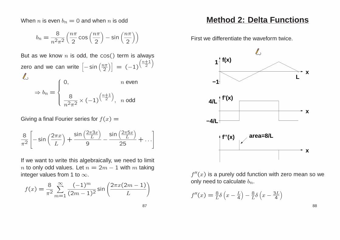
First we differentiate the waveform twice.
x
−1
1
Lx
−4/L
4/L
area=8/L
x
f(x)
f’(x)
f’’(x)
f ′′(x) is a purely odd function with zero mean so weonly need to calculate bn.
f ′′(x) = 8Lδ(
x− L4
)
− 8Lδ(
x− 3L4
)
88

To find the Fourier series for f ′′(x):
bn =2
L
∫ L
0sin
(
2πnx
L
)
f(x) dx
= 16L2
∫L0 sin
(
2πnxL
) [
δ(
x− L4
)
− δ(
x− 3L4
)]
dx
=16
L2
[
sin
(
2πnL
4L
)
− sin
(
6πnL
4L
)]
(sifting!)
=
0 , n even
32L2(−1)
(
n+32
)
, n odd
So the Fourier series for f ′′(x) =
32
L2
[
sin
(
2πx
L
)
− sin
(
6πx
L
)
+ sin
(
10πx
L
)
− . . .
]
We can also write this (note that 2m− 1 = n).
f ′′(x) =32
L2
∞∑
m=1
(−1)m+1 sin
(
2πx(2m− 1)
L
)
89
Now we integrate twice, each time setting the constantof integration to zero so we get a waveform with zeromean in each case.
f ′′(x) =32
L2
∞∑
m=1
sin
(
2πx(2m− 1)
L
)
(−1)m+1
f ′(x) =16
πL
∞∑
m=1
cos(
2πx(2m−1)L
)
2m− 1(−1)m
f(x) =8
π2
∞∑
m=1
sin(
2πx(2m−1)L
)
(2m− 1)2(−1)m
Which we can write out as follows f(x) =
8
π2
− sin
(
2πx
L
)
+sin
(
2π3xL
)
9−
sin(
2π5xL
)
25+ . . .
90
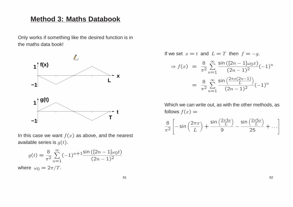
Method 3: Maths Databook
Only works if something like the desired function is inthe maths data book!
−1
1
Lx
f(x)
1
−1
tT
g(t)
In this case we want f(x) as above, and the nearestavailable series is g(t).
g(t) =8
π2
∞∑
n=1
(−1)n+1sin ([2n− 1]ω0t)
(2n− 1)2
where ω0 = 2π/T .
91
If we set x = t and L = T then f = −g.
⇒ f(x) =8
π2
∞∑
n=1
sin ([2n− 1]ω0x)
(2n− 1)2(−1)n
=8
π2
∞∑
n=1
sin(
2πx(2n−1)L
)
(2n− 1)2(−1)n
Which we can write out, as with the other methods, asfollows f(x) =
8
π2
− sin
(
2πx
L
)
+sin
(
2π3xL
)
9−
sin(
2π5xL
)
25+ . . .
92

Section 6: Summary
an =2
L
∫ L
0cos
(
2πnx
L
)
f(x) dx
bn =2
L
∫ L
0sin
(
2πnx
L
)
f(x) dx
d =1
L
∫ L
0f(x) dx
f(x) = d+∞∑
n=1
[
an cos
(
2πnx
L
)
+ bn sin
(
2πnx
L
)]
You can sometimes combine multiple integrals usingsymmetry properties.
Sometimes it is faster to calculate a related Fourierseries of delta functions and integrate.
Don’t forget the Fourier serieses given in the mathsdata book.
93
Section 7
Convergence & Half Range Serieses
The rule for predicting the convergence of the Fourierseries from the shape of the function is introduced.
This is used with the Fourier series for general periodto calculate serieses, valid over limited ranges, withimproved convergence properties. Four different se-rieses are calculated to model the same simple func-tion in order to illustrate this.
The usefulness of Matlab and Octave for numericalcalculation, and the use of Matlab for symbolic alge-bra are introduced.
94

General Range Example 3
A even function f(t) is periodic with period T = 2,and f(t) = cosh(t − 1) for 0 ≤ t ≤ 1. Sketchf(t) in the range −2 ≤ t ≤ 4. Find a Fourier seriesrepresentation for f(t).
First remember what the graph of cosh(t) looks like.
cosh(t)
t1
95
f(t)
t
−1−2 0 1 2 3 4
1
It is an even function ⇒ bn = 0 and an 6= 0. The
mean value of the function is non-zero ⇒ d 6= 0.
an =2
T
∫ 1
−1f(t) cos
(
2πnt
T
)
dt
=4
T
∫ 1
0f(t) cos
(
2πnt
T
)
dt
= 2
∫ 1
0cosh(t− 1) cos(nπt) dt
=2sinh(1)
1 + n2π2
96
d =1
T
∫ 1
−1f(t) dt =
2
T
∫ 1
0f(t) dt
=∫ 1
0cosh(t− 1) dt = sinh(1)
So
f(t) = d+∞∑
n=1
an cos
(
2πnx
L
)
= sinh(1)
1+ 2∞∑
n=1
cos(nπt)
1 + n2π2
97
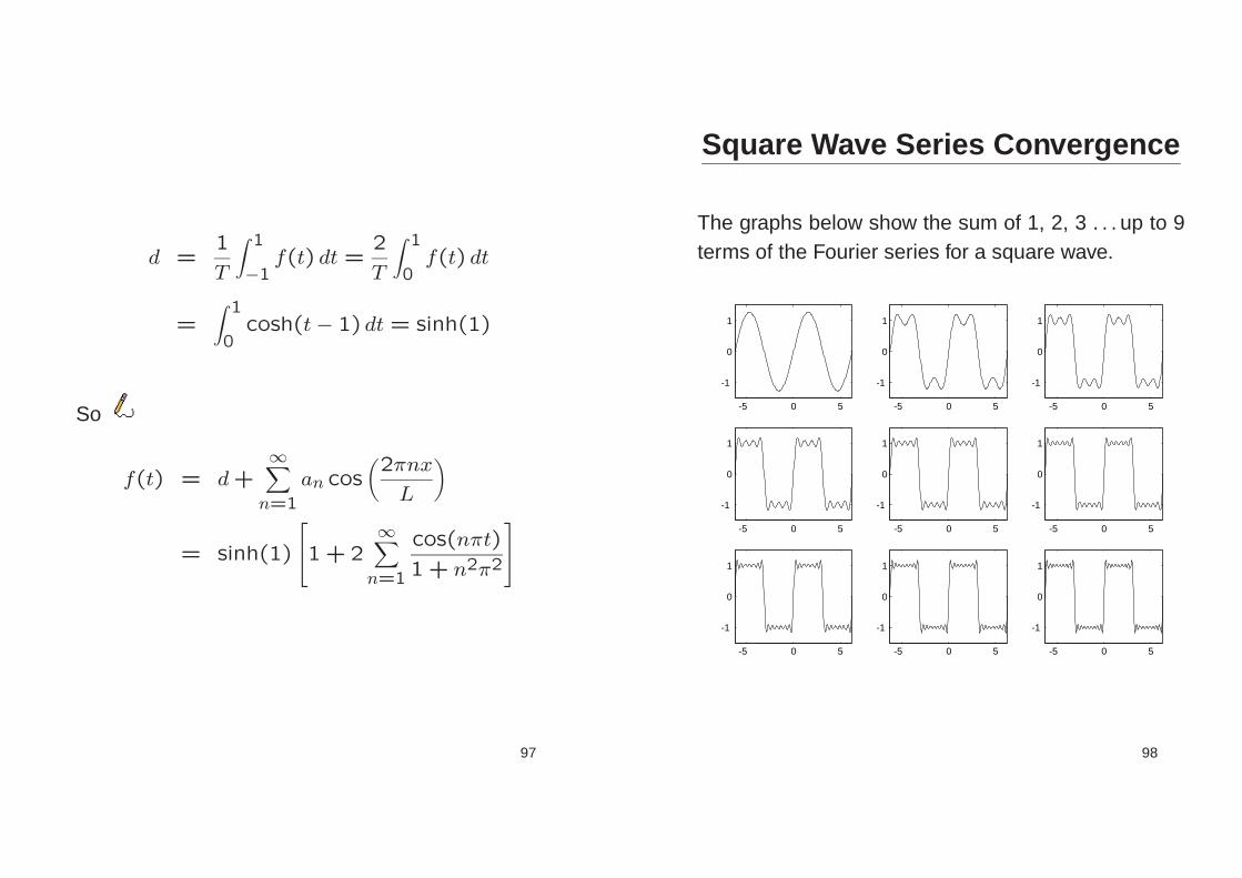
Square Wave Series Convergence
The graphs below show the sum of 1, 2, 3 . . . up to 9terms of the Fourier series for a square wave.
-5 0 5
-1
0
1
-5 0 5
-1
0
1
-5 0 5
-1
0
1
-5 0 5
-1
0
1
-5 0 5
-1
0
1
-5 0 5
-1
0
1
-5 0 5
-1
0
1
-5 0 5
-1
0
1
-5 0 5
-1
0
1
98
Using Matlab/Octave
% Fourier series for square wave
number = 200;
dtheta = 4 * pi/number;
theta = -2 * pi:dtheta:2 * pi;
nharm = 20;
d = 0;
thing = d * ones(1,number+1);
for n=1:nharm
if mod(n,2) == 1
bn = 4/(pi * n);
else
bn = 0;
end
an = 0;
thing = thing + an * cos(n * theta) ...
+ bn * sin(n * theta);
plot(theta,thing);
axis([-2 * pi 2 * pi -1.5 1.5]);
pause(1)
end
99
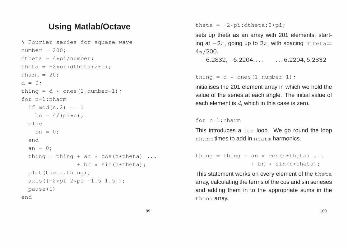
theta = -2 * pi:dtheta:2 * pi;
sets up theta as an array with 201 elements, start-ing at −2π, going up to 2π, with spacing dtheta =
4π/200.
−6.2832,−6.2204, . . . . . .6.2204,6.2832
thing = d * ones(1,number+1);
initialises the 201 element array in which we hold thevalue of the series at each angle. The initial value ofeach element is d, which in this case is zero.
for n=1:nharm
This introduces a for loop. We go round the loopnharm times to add in nharm harmonics.
thing = thing + an * cos(n * theta) ...
+ bn * sin(n * theta);
This statement works on every element of the theta
array, calculating the terms of the cos and sin seriesesand adding them in to the appropriate sums in thething array.
100

Using Matlab Symbolic ToolsBoth convolution and Fourier work involves a lot of in-tegration. Sometimes it is nice to know what the rightanswer is, so you can check your working. To inte-grate p with respect to x from a to b you use the com-mand int(p, x, a, b) . Consider the integral:
2
T
∫ T
0cos
(
2πnx
T
)
x dx = 0
>> syms n x T>> int((2/T) * x* cos(2 * pi * n* x/T),x,0,T)
ans =T* (cos(pi * n)ˆ2-1
+2* pi * n* sin(pi * n) * cos(pi * n))/piˆ2/nˆ2
which is
T(
(cos(π n))2 − 1+ 2π n sin(π n) cos(π n))
π2n2
But as n is an integer, cos2(nπ) = 1 and sin(nπ) =
0, so the integral evaluates to zero.
Don’t rely on this too much. You need to be able tointegrate efficiently by hand in the exam.
101
Convergence Examples
−π π
1−1
f(t)
t2π−2π
The Fourier series for asquare wave converges as1/n. Notice that it is dis-
continuous of value.
f(t) =4
π
[
sin(t) +sin(3t)
3+
sin(5t)
5+ . . .
]
π2
t−π π
F(t)The Fourier series for a tri-angular wave converges as1/n2. It is continuous ofvalue, but discontinuous of
gradient.
F(t) =−4
π
[
cos(t) +cos(3t)
9+
cos(5t)
25+ . . .
]
102
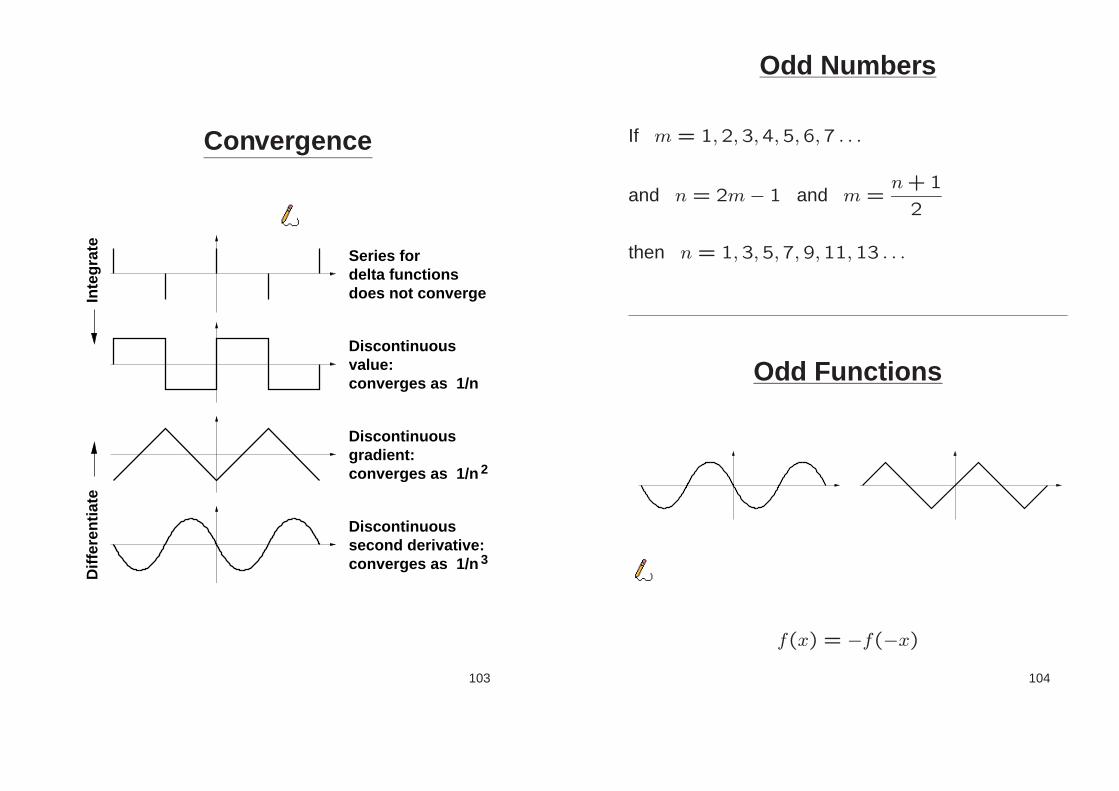
Convergence
Discontinuoussecond derivative:converges as 1/n 3
Series fordelta functionsdoes not converge
Discontinuousvalue:converges as 1/n
Discontinuousgradient:converges as 1/n 2
Inte
grat
eD
iffer
entia
te
103
Odd Numbers
If m = 1,2,3,4,5,6,7 . . .
and n = 2m− 1 and m =n+1
2
then n = 1,3,5,7,9,11,13 . . .
Odd Functions
f(x) = −f(−x)
104

“Half Range” Series
If we want to model a signal f(x) = x in the range0 to T . We can use the Fourier formulae for generalrange to generate a variety of different serieses. Theywill all be the same in the range 0 to T , but some mayconverge faster than others.
Full range seriesperiod Tconverges as 1/n
Cosine seriesperiod 2T, b = 0nconverges as 1/n 2
T 2T−T−2T
Sine series
converges as 1/nn
2
Sine series
converges as 1/nn
period 4T, a = 0, d = 0
period 2T, a = 0, d = 0
105
Normal Series, Period T
−T−2T T 2T
T
x
f(x)Find the Fourier series tomodel f(x) = x from 0 toT , using a series of periodT .
an =2
T
∫ T
0cos
(
2πnx
T
)
x dx = 0
bn =2
T
∫ T
0sin
(
2πnx
T
)
x dx =−T
nπ
d =1
T
∫ T
0x dx =
T
2
⇒ f(x) =T
2−
∞∑
n=1
T
nπsin
(
2πnx
T
)
Notice that the series converges as 1/n.
106
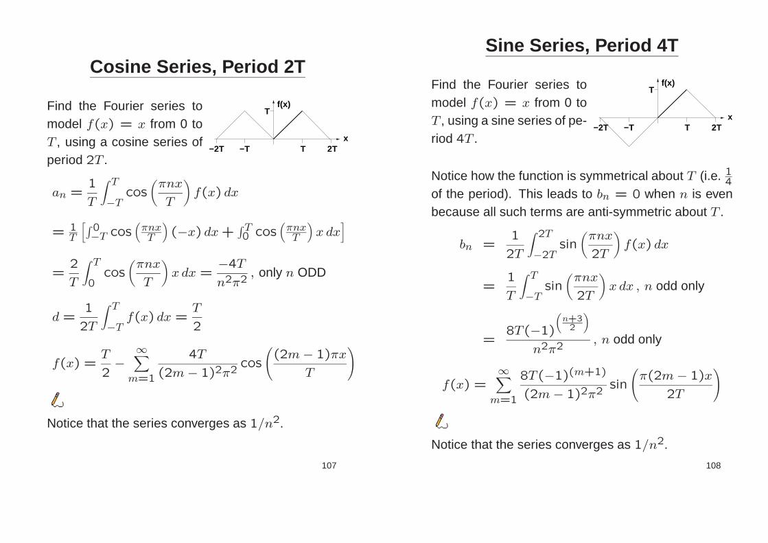
Cosine Series, Period 2T
−T−2T T 2T
T
x
f(x)Find the Fourier series tomodel f(x) = x from 0 toT , using a cosine series ofperiod 2T .
an =1
T
∫ T
−Tcos
(
πnx
T
)
f(x) dx
= 1T
[
∫ 0−T cos
(
πnxT
)
(−x) dx+∫ T0 cos
(
πnxT
)
x dx]
=2
T
∫ T
0cos
(
πnx
T
)
x dx =−4T
n2π2, only n ODD
d =1
2T
∫ T
−Tf(x) dx =
T
2
f(x) =T
2−
∞∑
m=1
4T
(2m− 1)2π2cos
(
(2m− 1)πx
T
)
Notice that the series converges as 1/n2.
107
Sine Series, Period 4T
−T−2T T 2T
T
x
f(x)Find the Fourier series tomodel f(x) = x from 0 toT , using a sine series of pe-riod 4T .
Notice how the function is symmetrical about T (i.e. 14
of the period). This leads to bn = 0 when n is evenbecause all such terms are anti-symmetric about T .
bn =1
2T
∫ 2T
−2Tsin
(
πnx
2T
)
f(x) dx
=1
T
∫ T
−Tsin
(
πnx
2T
)
x dx , n odd only
=8T(−1)
(
n+32
)
n2π2, n odd only
f(x) =∞∑
m=1
8T(−1)(m+1)
(2m− 1)2π2sin
(
π(2m− 1)x
2T
)
Notice that the series converges as 1/n2.
108

Sine Series, Period 2T
−T−2T T 2T
T
x
f(x)Find the Fourier series tomodel f(x) = x from 0 toT , using a sine series of pe-riod 2T .
bn =1
T
∫ T
−Tsin
(
πnx
T
)
x dx
=−2T
nπ(−1)n
⇒ f(x) =∞∑
n=1
−2T
nπ(−1)n sin
(
πnx
T
)
Notice that the series converges as 1/n.
109
Section 7: Summary
Discontinuoussecond derivative:converges as 1/n 3
Series fordelta functionsdoes not converge
Discontinuousvalue:converges as 1/n
Discontinuousgradient:converges as 1/n 2
Inte
grat
eD
iffer
entia
te
If you are modelling a limited section of a function, pickthe Fourier series period so as to get good conver-gence and a series that is easy to calculate (i.e. someof an, bn or d zero).
110

Section 8
Complex Fourier Series
The complex Fourier series is presented first with pe-riod 2π, then with general period.
The connection with the real-valued Fourier series isexplained and formulae are given for converting be-tween the two types of representation.
Examples are given of computing the complex Fourierseries and converting between complex and real se-rieses.
111
New Basis Functions
Recall that the Fourier series builds a representationcomposed of a weighted sum of the following basisfunctions.
1 (i.e. a constant term)cos(t) cos(2t) cos(3t) cos(4t) . . .sin(t) sin(2t) sin(3t) sin(4t) . . .
Computing the weights an, bn and d often involvessome nasty integration.
We now present an alternative representation basedon a different set of basis functions:
1 (i.e. a constant term)eit e2it e3it e4it . . .e−it e−2it e−3it e−4it . . .
These can all be represented by the term
eint
with n taking integer values from −∞ to +∞. Notethat the constant term is provided by the case whenn = 0.
112

Series of Complex Exponentials
A representation based on this family of functions iscalled the “complex Fourier series”.
f(t) =∞∑
n=−∞cne
int
The coefficients, cn, are normally complex numbers.
It is often easier to calculate than the sin/cos Fourierseries because integrals with exponentials in are usu-ally easy to evaluate.
We will now derive the complex Fourier series equa-tions, as shown above, from the sin/cos Fourier seriesusing the expressions for sin() and cos() in terms ofcomplex exponentials.
113
Complex Fourier Series
f(t) = d+∞∑
n=1
[an cos(nt) + bn sin(nt)]
= d+∞∑
n=1
[
an
(
eint + e−int
2
)
+ bn
(
eint − e−int
2i
)]
= d+∞∑
n=1
(an − ibn)
2eint +
∞∑
n=1
(an + ibn)
2e−int
=∞∑
n=−∞cne
int
where
cn =
d , n = 0
(an − ibn) /2 , n = 1,2,3, . . .(a−n + ib−n) /2 , n = −1,−2,−3, . . .
Note that a−n and b−n are only defined when n isnegative.
114

an = 1π
∫ π−π cos(nt)f(t) dt
bn = 1π
∫ π−π sin(nt)f(t) dt
d = 12π
∫ π−π f(t) dt
thus for n positive
cn =1
2(an − ibn)
=1
2π
∫ π
−π[cos(nt)− i sin(nt)] f(t) dt
=1
2π
∫ π
−πe−intf(t) dt
for n negative
cn =1
2(a−n + ib−n)
=1
2π
∫ π
−π[cos(−nt) + i sin(−nt)] f(t) dt
=1
2π
∫ π
−πe−intf(t) dt
and for n = 0
c0 = d
=1
2π
∫ π
−πe−0f(t) dt
115
Complex Fourier Series Summary
cn =1
2π
∫ π
−πe−intf(t) dt
f(t) =∞∑
n=−∞cne
int
116

Complex Series Example 1
Find the complex Fourier series to model f(t) = sin(t).
cn =1
2π
∫ π
−πe−intf(t) dt
=1
2π
∫ π
−πe−int sin(t) dt
=1
2π
[
einπ − e−inπ
n2 − 1
]
Which is zero when n does not equal 1 or −1. Forthese two special cases we have to set n = 1 + ǫand calculate the limit of cn as ǫ tends to zero. Thisgives us
c1 =1
2i
c−1 =−1
2iWhich means the complex Fourier series for f(t) =
sin(t) is
f(t) =∞∑
n=−∞cne
int
=eit − e−it
2i
117
Finding the limit as n tends to 1
cn =1
2π
[
einπ − e−inπ
n2 − 1
]
Set n = 1+ ǫ and let ǫ tend to zero.
c1 =1
2π
eiπ(1+ǫ) − e−iπ(1+ǫ)
(1 + ǫ)2 − 1
=1
2π
[
−eiπǫ + e−iπǫ
(1 + ǫ)2 − 1
]
≈ 1
2π
[−1− iπǫ+1− iπǫ
1+ 2ǫ− 1
]
≈ 1
2π
[−2iπǫ
2ǫ
]
≈ −i
2
≈ 1
2i
118

Complex Series Example 2
x2πT
1f(x)Find the complex Fourier
series to model f(x) thathas a period of 2π and is 1when 0 < x < T and zerowhen T < x < 2π.
cn =1
2π
∫ 2π
0e−intf(t) dt
=i
2πn
[
e−inT − 1]
, when n 6= 0
=1
2πarea =
T
2π, when n = 0
So the Fourier series is
f(t) =∞∑
n=−∞cne
int
=1
2π
T +−1∑
n=−∞
i
n
[
e−inT − 1]
eint
+∞∑
n=1
i
n
[
e−inT − 1]
eint
119
Converting c to a, b and d
From our example on the previous page.
cn =
i2πn
[
e−inT − 1]
, when n 6= 0
12πarea = T
2π , when n = 0
We wish to calculate the coefficients for the equivalentFourier series in terms of sin() and cos().
Clearly d = c0 = T2π . For n > 0
cn = (an − ibn)/2
⇒ an = 2Re{cn}and bn = −2 Im{cn}
converting our expression for cn into sin() and cos():
2cn =i
πn[cos(nT)− i sin(nT)− 1]
=1
πn[sin(nT) + i(cos(nT)− 1)]
so an =sin(nT)
nπand bn =
1− cos(nT)
nπ.
120

Complex Fourier Series
f(t) =1
2π
T +−1∑
n=−∞
i
n
[
e−inT − 1]
eint
+∞∑
n=1
i
n
[
e−inT − 1]
eint
Real Fourier Series
f(t) =T
2π+
∞∑
n=1
sin(nT)
nπcos(nt)
+∞∑
n=1
1− cos(nT)
nπsin(nt)
Both serieses converge as 1/n.
121
Converting from Real to Complex
−π π
1−1
f(t)
t2π−2π
Convert the real Fourier se-ries of the square wavef(t) to a complex series.
For the real series, we know that d = an = 0 and
bn =1
π
∫ π
−πsin(nt)f(t) dt =
4
nπ, n odd
giving f(t) = 4π
[
sin(t) + sin(3t)3 + sin(5t)
5 + . . .]
To convert to a complex series, use
cn =
d , n = 0
(an − ibn) /2 , n = 1,2,3, . . .(a−n + ib−n) /2 , n = −1,−2,−3, . . .
so we havec0 = 0cn = −2i/(nπ) , n positive and oddcn = 2i/(−nπ) , n negative and |n| odd
⇒ f(t) =−2i
π
[
. . .+e−5it
−5+
e−3it
−3+
e−it
−1
+eit
1+
e3it
3+
e5it
5+ . . .
]
122
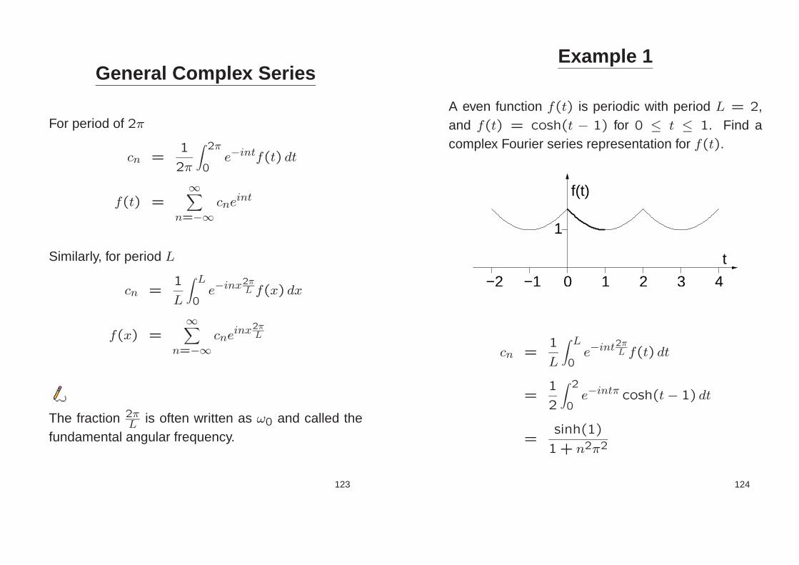
General Complex Series
For period of 2π
cn =1
2π
∫ 2π
0e−intf(t) dt
f(t) =∞∑
n=−∞cne
int
Similarly, for period L
cn =1
L
∫ L
0e−inx2π
L f(x) dx
f(x) =∞∑
n=−∞cne
inx2πL
The fraction 2πL is often written as ω0 and called the
fundamental angular frequency.
123
Example 1
A even function f(t) is periodic with period L = 2,and f(t) = cosh(t − 1) for 0 ≤ t ≤ 1. Find acomplex Fourier series representation for f(t).
f(t)
t
−1−2 0 1 2 3 4
1
cn =1
L
∫ L
0e−int2πL f(t) dt
=1
2
∫ 2
0e−intπ cosh(t− 1) dt
=sinh(1)
1 + n2π2
124

Hence the complex Fourier series is
f(t) =∞∑
n=−∞cne
int2πL
=∞∑
n=−∞
sinh(1)eintπ
1+ n2π2
We can check this answer by computing the equiv-alent real Fourier series which we calculated at thestart of section 7.
an = 2Re{cn} , n = 1,2,3, . . .bn = −2 Im{cn} , n = 1,2,3, . . .d = c0
In this case, as cn is entirely real,
an = 2cn =2sinh(1)
1 + n2π2, n = 1,2,3, . . .
bn = 0
d = sinh(1)
125
Example 2
1−1−L
L
f(x)
x
Find the complex Fourierseries of the the squarewave f(x).
Note that the mean of the function is zero, so c0 = 0.
cn =1
L
∫ L
0e−inx2π
L f(x) dx
=1
L
[
∫ L/2
0e−inx2π
L dx−∫ L
L/2e−inx2π
L dx
]
=1
2inπ
[
e−2inπ +1− 2e−inπ]
f(x) =∞∑
n = −∞n 6= 0
[
1− e−inπ]
inπeinx
2πL
f(x) =2
iπ
. . .+e−5ix2π
L
−5+
e−3ix2πL
−3+
e−ix2πL
−1
+eix
2πL
1+
e3ix2πL
3+
e5ix2πL
5+ . . .
126

Converting to a Real Series
We wish to convert the complex general range squarewave series into a series with real coefficients.
cn =
{
2/(inπ) , |n| odd0 , |n| even
Clearly d = c0 = 0. For a and b use:
cn = (an − ibn)/2
⇒ an = 2Re{cn} = 0
and bn = −2 Im{cn} =4
nπ, n odd
Which gives us the real series:
f(t) =4
π
sin
(
x2π
L
)
+sin
(
3x2πL
)
3
+sin
(
5x2πL
)
5+ . . .
127
Section 8: Summary
For period L
cn =1
L
∫ L
0e−inx2π
L f(x) dx
f(x) =∞∑
n=−∞cne
inx2πL
Relationship with the cos/sin Fourier series.
cn =
d , n = 0
(an − ibn) /2 , n = 1,2,3, . . .(a−n + ib−n) /2 , n = −1,−2,−3, . . .
an = 2Re{cn} , n = 1,2,3, . . .bn = −2 Im{cn} , n = 1,2,3, . . .d = c0
128

Section 9
Probability
In this section we summarise the key issues in pages1–13 of the basic probability teach-yourself documentand provide a single simple example of each concept.
This presentation is intended to be reinforced by themany examples in the teach-yourself document andthe first 12 questions of examples paper 10.
129
Probability
Probability of A =
Number of outcomes for which A happensTotal number of outcomes (sample space)
What is the probability of drawing an ace from a shuf-fled pack of cards?
There are 4 aces. There are 52 cards in total. There-fore the probability is
P( ace ) =4
52=
1
13
130

Adding Probabilities
P(A or B) = P(A) + P(B)
provided A and B cannot happen together, i.e. A andB must be mutually exclusive outcomes.
What is the probability of drawing an ace or a kingfrom a shuffled pack of cards?
P( ace ) =1
13
P( king ) =1
13
⇒ P( ace or king ) =1
13+
1
13=
2
13
131
When Not to Add Probabilities
When the events are not mutually exclusive.
A and B
= A or BA B
P(A or B) = P(A) + P(B)− P(A and B)
132

Non-Exclusive Events
What is the probability of drawing an ace or a spadefrom a shuffled pack of cards?
P( ace ) =1
13P( spade ) =
13
52=
1
4
but P( ace or spade ) is not the sum of these valuesbecause the outcomes “ace” and “spade” are not ex-clusive; it is possible to have them both together bydrawing the ace of spades.
To calculate P( ace or spade )
either use the formula from the previous slide:
P( ace ) + P( spade ) − P( ace of spades )1
13+
1
4− 1
52=
4
13
or use the original definition of probability.
number of aces and spades
total number of cards=
4+ 13− 1
52=
4
13
133
Multiplying Probabilities
P(A and B) = P(A)× P(B)
provided A is not affected by the outcome of B and B
is not affected by the outcome of A, i.e. A and B mustbe independent.
I have two shuffled packs of cards and draw a cardfrom each of them. What is the probability that I drawtwo aces?
P( ace ) =1
13
P( ace and ace ) =1
13× 1
13=
1
169
134

Non-independent Events
I have a single pack of cards. I draw a card, then drawa second card without putting the first card back in thepack. What is the probability that I draw two aces?
This time the probability that I get an ace as the sec-ond card is affected by whether or not I removed anace from the pack when I drew the first card.
We use the notation P(B|A) to denote the probabilitythat B happens, given that we know that A happened.This is called a conditional probability.
P(A and B) = P(A|B)P(B)
Thus:
P( [second = ace] and [first = ace] )
= P( second = ace | first = ace )P( first = ace )
135
Tree Diagram
We can use a tree diagram to help us work this out.
NotAce
NotAce
NotAce
6633
663564
66348
66348
1221
Ace
Ace
Ace
1/13
12/13
3/51
48/51
4/51
47/51
=
First card Second card
The probability that both cards are aces = 1221.
136

Another Example
I have a single pack of cards. I draw a card, then drawa second card without putting the first card back in thepack. What is the probability that the second card isan ace, given that the first card was not an ace?
NotAce
NotAce
NotAce
Ace
Ace
Ace
1/13
12/13
3/51
48/51
4/51
47/51
Second cardFirst card
P( second = ace | first = not ace ) = 451
137
Notation
Intersection⋂
AND
Union⋃
OR
Thus the conditional probability formula
P(A and B) = P(A|B)P(B)
is more normally written
P(A ∩B) = P(A|B)P(B)
and instead of
P(A or B) = P(A) + P(B)− P(A and B)
we write
P(A ∪B) = P(A) + P(B)− P(A ∩B)
138

Ordering Objects
The number of different orders in which n unique ob-jects can be placed is n! (n factorial)
I have three cards with values 2, 3 and 4. They areshuffled into a random order. What is the probabilitythey are in the order 2, 3, 4?
The number of possible orders for three cards is 3!
The probability the cards are found in one specific or-der is therefore 1
3! =16.
139
Permutations
nPr =n!
(n− r)!
is the number of ways of choosing r items from n
when the order of the chosen items matters.
Ten people are involved in a race. I wish to make aposter for every possible winning combination of gold,silver and bronze medal winners. How many posterswill I need?
We need to know the number of ways of choosingthree people out of 10, taking account of the order.This is
10P3 =10!
7!= 10× 9× 8 = 720
So I would need rather a lot of posters.
140

Combinations
nCr =n!
(n− r)!r!
is the number of ways of choosing r items from n
when the order of the chosen items does not matter.
I have a single pack of cards. I draw a card, then drawa second card without putting the first card back in thepack. What is the probability that I draw two aces?
The number of ways of drawing 2 cards from 52 is
52C2.
The number of ways of getting two aces is the numberof ways of drawing 2 aces from the 4 aces in the pack.This is 4C2.
The probability that I draw two aces is therefore
num ace pairs
num pairs=
4C2
52C2=
4!
2! 2!× 50! 2!
52!
=4× 3
52× 51=
1
221
141
Lottery Example 1
What is the probability of winning the jackpot in thenational lottery? There are 49 balls and you have tomatch all six to win.
Method 1:
6
49× 5
48× 4
47× 3
46× 2
45× 1
44=
1
13983816
Method 2:
1number of ways of choosing 6 balls from49, where order does not matter
=1
49C6
1
49C6=
6!43!
49!=
6× 5× 4× 3× 2× 1
49× 48× 47× 46× 45× 44
=1
13983816
142

Lottery Example 2
What is the probability of winning £10 by matching ex-actly 3 balls in the national lottery
Method 1:
Work out the probability of matching them in a par-ticular order: the first 3 balls that are drawn win, theremaining 3 do not.
6
49× 5
48× 4
47× 43
46× 42
45× 41
44
Then multiply this by the number of possible ways ofpicking the 3 winning balls among the 6 balls that aredrawn.
✔ ✔ ✔ ✖ ✖ ✖
✔ ✔ ✖ ✔ ✖ ✖
✔ ✔ ✖ ✖ ✔ ✖
✔ ✔ ✖ ✖ ✖ ✔
✔ ✖ ✔ ✔ ✖ ✖
. . . etc.
6C3 = 20
Hence:6
49× 5
48× 4
47×43
46×42
45×41
44× 6C3 =
1
56.7
143
Matching only 3 balls, method 2:
number of ways we can win
total possible number of outcomes
Thinking about all the balls in the lottery machine, weconsider:
The number of ways thelottery machine can pick3 balls matching someof the 6 numbers on ourticket.
The number of ways thelottery machine can pick3 balls from the 43 ballsnot on our ticket.
(
The total number of ways of picking 6balls out of the 49 in the machine.
)
=6C3 43C3
49C6=
6!43! 43! 6!
49! 40! 3! 3! 3!
=43× 42× 41× 6× 5× 4× 6× 5× 4
49× 48× 47× 46× 45× 44× 3× 2
=1
56.7
144

Section 9: Summary
P(A ∪ B) = P(A) + P(B) if A and B are mutuallyexclusive outcomes.
P(A ∩ B) = P(A) × P(B) provided A and B areindependent.
P(A ∩B) = P(A|B)P(B)
P(A ∪B) = P(A) + P(B)− P(A ∩B)
The number of different orders in which n unique ob-jects can be placed is n!
Permutations: nPr = n!(n−r)!
is the number of ways ofchoosing r items from n when the order of the chosenitems matters.
Combinations: nCr = n!(n−r)!r!
is the number of waysof choosing r items from n when the order of the cho-sen items does not matter.
145
Section 10
Statistics
In this section we summarise the key issues in pages14–20 of the basic probability teach-yourself docu-ment. This presentation is intended to be reinforcedby the examples in the teach-yourself document andquestions 13 and 14 in examples paper 9.
The main focus is on the mean and standard deviationof a probability distribution. We also explain how tocalculate a range within which we are (say) 95% surethat the true value of an experimental reading will lie.
146

Mean
The mean µ, of a population of values xi (where i
goes from 1 to N ), is defined.
µ =Sum of all the values
Number of values=
∑Ni=1 xiN
Imagine a pack of cards with all the jokers and picturecards removed. We are only concerned with the nu-merical value of the cards. We have four each of allthe numbers from one to ten so N = 40.
Arithmetic mean: µ =
∑Ni=1 xi
N=
220
40= 5.5
The mean is a measure of the central tendency orlocation of the population.
147
Variance & Standard Deviation
Variance and standard deviation are measures of thespread of the distribution. The variance is the aver-age squared difference between each value and themean. The population variance is usually given thesymbol σ2.
Variance: σ2 =
∑Ni=1(xi − µ)2
N
The standard deviation (SD) is the square root of thevariance. The population standard deviation is usuallygiven the symbol σ.
Standard Deviation: σ =
√
∑Ni=1(xi − µ)2
N
We can work out the variance and standard deviationof the values on our set of forty cards.
σ2 =
∑Ni=1(xi − µ)2
N=
330
40= 8.25
σ =
√
330
40= 2.8723
148

Sample
Until now we have assumed that we can see all thecards at once. Now we are going to change the game.Imagine that someone else is holding the cards andallowing us to pick one at random, note its value andthen replace it. Using this pick-and-replace processwe can view a sample of the cards. This sample canbe of any size as the cards are picked at random andreplaced. Assume that the sample size is n.
The challenge is to estimate the mean and standarddeviation of the original numbers on the cards basedonly on what we see in the sample. Here are the for-mulae that enable us to do this.
Estimate of Mean (based on sample):
m =
∑ni=1 xin
Estimate of Standard Deviation (based on sample):
s =
√
√
√
√
∑ni=1(xi −m)2
n− 1
149
Convenient Formula for s
In the literature, s, the standard deviation of the un-derlying population estimated from a sample is calledthe “sample standard deviation”.
There is a convenient formula for calculating s.
s =
√
√
√
√
∑ni=1(xi −m)2
n− 1
=
√
√
√
√
√
(
∑ni=1 x
2i
)
− 1n
(
∑ni=1 xi
)2
n− 1
150

Standard Deviation from a Sample
Ten cards are selected individually from our specialreduced pack of 40 cards (described on slide 147),noted and replaced in the pack. This gives a samplesize n = 10. The values of the cards are:
10 3 4 3 54 1 5 8 5
We wish to estimate the mean m, and standard devi-ation s, of the values on all the cards, based only onknowledge of this sample.
m =
∑ni=1 xin
=48
10= 4.8
s =
√
√
√
√
√
(
∑ni=1 x
2i
)
− 1n
(
∑ni=1 xi
)2
n− 1
=
√
√
√
√
(290)− 110 (48)2
9= 2.5734
151
Discrete Probability Distribution
Consider picking a card (from the pack described onslide 147), noting its value and then replacing it in thepack. We can compute the probability of picking eachof the possible values.
Probability of value on card
1 2 3 4 5 6 7 8 9 10
0.1
x
Value on the card
P(x)
This is a probability distribution. In this case it is adiscrete distribution because the cards can only carrycertain integer values. Notice that the sum of all thehistogram bars is 10 × 0.1 = 1. There are ten pos-sible outcomes and they each have a probability of1/10. This is called a uniform distribution.
152

Mean and SD from the Distribution
The probability distribution is a property of the pop-ulation of the numbers on the cards. Knowing thecomplete probability distribution enables us to calcu-late the mean µ and the standard deviation σ exactly.
Let xj represent each of the different values that areprinted on the cards and M equal the number of thesedifferent values. In our example M = 10.
Arithmetic mean: µ =M∑
j=1
xjP(xj)
Variance: σ2 =M∑
j=1
(xj − µ)2P(xj)
Standard Deviation: σ =
√
√
√
√
√
M∑
j=1
(xj − µ)2P(xj)
153
Example
Probability of value on card
1 2 3 4 5 6 7 8 9 10
0.1
x
Value on the card
P(x)
We can see from the histogram that P(xj) = 0.1 forall the values on the cards (i.e. for all j). In this partic-ular case, the values xj are the same numerically asthe index j, so we can substitute xj = j. Hence
µ =M∑
j=1
xjP(xj) =10∑
j=1
j × 0.1 = 5.5
Now we use this value of µ in the formula for standarddeviation.
σ =
√
√
√
√
√
M∑
j=1
(xj − µ)2P(xj)
=
√
√
√
√
√
10∑
j=1
(j − 5.5)2 × 0.1 = 2.8723
154

Continuous Probability Distribution
If you have an outcome that can take any real value(rather than a finite number of discrete values) this canbe described by a probability density function (PDF).
1 2 3 4 5 6 7 8 9 10
x
Value
Probability density function
f(x)
Here the total area under the curve must be 1 and theprobability of x taking a value in the range from (say)6 to 7 is given by the integral (i.e. area) between 6 and7. More generally:
The probability of (a < x < b) =
∫ b
af(x) dx
Examples of continuous random variables: the weightof a sample, the time for a physical process to com-plete, an output voltage.
155
Mean and SD from PDF
It is also possible to calculate the mean (µ) and stan-dard deviation (σ) of a distribution from its probabilitydensity function.
µ =∫ +∞
−∞xf(x) dx
σ =
√
∫ +∞
−∞(x− µ)2f(x) dx
Knowing the probability density function enables usto calculate the mean µ and the standard deviation σ
exactly.
156

Example using a PDF
Consider a machine than makes widgets which aresupposed to be a particular length. Unfortunately, themachine often makes widgets that are slightly too long;it never makes widgets that are too short. The graphbelow shows the probability density function for thenumber of millimetres that a widget is too long.
1 2 3 4 5 6 7 8 9 10
x
Value
Probability density function
f(x)
0
0.2
0.0
157
Widget Example 1
1. What is the probability that a widget is less than1 mm too long?For 0 ≤ x ≤ 10 we can see that f(x) = 0.2−0.02x,hence:
P(0 < x < 1) =∫ 1
0f(x) dx
=
∫ 1
00.2− 0.02x dx = 0.19
So the probability of a widget being less than 1 mmtoo long is 0.19.
2. Calculate the mean and standard deviation of thedistribution of excess lengths.
µ =
∫ 10
0x(0.2− 0.02x) dx = 3.3333
σ =
√
∫ 10
0(x− 10/3)2(0.2− 0.02x) dx = 2.3570
158

Widget Example 2
3. What is the probability that a widget is producedwith an excess length within one standard deviationfrom the mean excess length?We wish to calculate the probability of an excess lengthin the range 3.33 − 2.36 to 3.33 + 2.36, which isgiven by:
P(x within one σ of µ) =
∫ 5.6904
0.97630.2− 0.02x dx
= 0.6285
4. The manufacturer wants to quote an excess lengththat he is sure 95% of the widgets produced will beshorter than. What should it be?We need to solve for d in:
0.95 =
∫ d
00.2− 0.02x dx
⇒ 0.95 = 0.2d− 0.01d2
So d = 10−√5 = 7.7639 mm
159
Standard Deviation of Sample Mean
Suppose x is a random variable withmean = µ
standard deviation = σ
We have n samples of x: [x1, x2, x3, . . . xn].
Let x be the average of these samples =n∑
i=1
xin
.
Now the key point is that x is also a random variable.
The mean of x is µ.
The standard deviation of x isσ√n
.
160
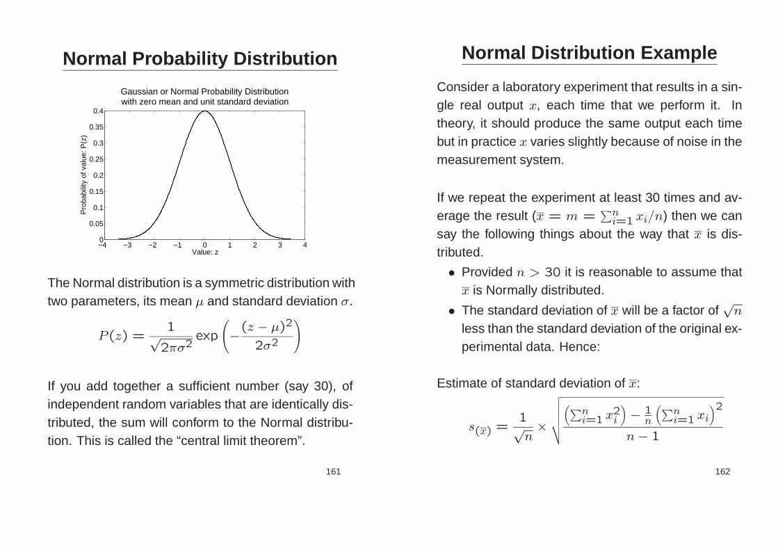
Normal Probability Distribution
−4 −3 −2 −1 0 1 2 3 40
0.05
0.1
0.15
0.2
0.25
0.3
0.35
0.4
Value: z
Pro
babi
lity
of v
alue
: P(z
)Gaussian or Normal Probability Distributionwith zero mean and unit standard deviation
The Normal distribution is a symmetric distribution withtwo parameters, its mean µ and standard deviation σ.
P(z) =1√2πσ2
exp
(
−(z − µ)2
2σ2
)
If you add together a sufficient number (say 30), ofindependent random variables that are identically dis-tributed, the sum will conform to the Normal distribu-tion. This is called the “central limit theorem”.
161
Normal Distribution Example
Consider a laboratory experiment that results in a sin-gle real output x, each time that we perform it. Intheory, it should produce the same output each timebut in practice x varies slightly because of noise in themeasurement system.
If we repeat the experiment at least 30 times and av-erage the result (x = m =
∑ni=1 xi/n) then we can
say the following things about the way that x is dis-tributed.
• Provided n > 30 it is reasonable to assume thatx is Normally distributed.
• The standard deviation of x will be a factor of√n
less than the standard deviation of the original ex-perimental data. Hence:
Estimate of standard deviation of x:
s(x) =1√n×
√
√
√
√
√
(
∑ni=1 x
2i
)
− 1n
(
∑ni=1 xi
)2
n− 1
162

Normal Distribution Example 2
If it is fair to assume that the error in the original exper-imental data is unbiased, then the standard deviationof x gives us useful information about the error it islikely to contain.
Let s(x) be our estimate of the standard deviation of xand let X be the (unknown) true value of the thing weare intending to measure.
50% of the time, x will lie within 0.67s(x) of X68% of the time, x will lie within s(x) of X95% of the time, x will lie within 2s(x) of X99.73% of the time, x will lie within 3s(x) of X
−4 −3 −2 −1 0 1 2 3 40
0.05
0.1
0.15
0.2
0.25
0.3
0.35
0.4
Value: z
Pro
babi
lity
of v
alue
: P(z
)
Gaussian or Normal Probability Distributionwith zero mean and unit standard deviation
Value: zx
68% ofarea lieswithin one SD of themean
χ
163
Normal Distribution Example 3
−4 −3 −2 −1 0 1 2 3 40
0.05
0.1
0.15
0.2
0.25
0.3
0.35
0.4
Value: z
Pro
babi
lity
of v
alue
: P(z
)
Gaussian or Normal Probability Distributionwith zero mean and unit standard deviation
xTruevalue
Mean of recordeddata
χ
area lieswithin
of themean
95% of
two SDs
Value: z
If we repeat an experiment 30 times and
• the average result x = 3.0279,• we calculate an estimate of the standard devia-
tion of the experimental error as 0.2036• then our estimate of the standard deviation of x
will be 0.2036/√30 = 0.0372.
The true experimental result will have a 95% chanceof lying within two standard deviations from the mean,i.e. in the range from 2.9536 to 3.1023.
164

Section 10: Summary
PDF probability density functionSD standard deviationµ mean of a distribution (or from a PDF)σ2 variance of a distribution (or from a PDF)σ SD of a distribution (or from a PDF)m = x estimate of µ based on a sample of x valuess estimate of σ based on a sample of x valuess(x) estimate of SD of x based on sample of x
s(x) = s/√n where n is the sample size.
If we are prepared to do an experiment at least 30times and believe our results to be unbiased, we canuse the “central limit theorem” together with the shapeof the Normal distribution to calculate a range withinwhich the true result is likely to lie. We can make astatement of the form: “There is a probability of blahthat the true result lies between blah and blah.” Thisis called a confidence interval.
165
Acknowledgements
These notes are inspired by Prof Woodhouse’s notesfor the same course and incorporate several sugges-tions from Drs Gee and Treece. I am very gratefulto Martin Weber and Naveed Ahmad for checking thealgebra in the examples.
166


