
Model reduction of large-scale dynamical systemsLecture III: Krylov approximation and rational interpolation
Thanos Antoulas
Rice University and Jacobs University
email: [email protected]: www.ece.rice.edu/ aca
International School, Monopoli, 7 - 12 September 2008
Thanos Antoulas (Rice U. & Jacobs U.) Reduction of large-scale systems 1 / 38

Outline
1 Krylov approximation methods
2 The Arnoldi and the Lanczos proceduresThe Arnoldi procedureThe Lanczos procedureAn example
3 Krylov methods and moment matchingRemarks
4 Rational interpolation by Krylov projectionRealization by projectionInterpolation by projection
5 Choice of Krylov projection points: Optimal H2 model reduction
6 Summary: Lectures II and III
Thanos Antoulas (Rice U. & Jacobs U.) Reduction of large-scale systems 2 / 38
Krylov approximation methods
Outline
1 Krylov approximation methods
2 The Arnoldi and the Lanczos proceduresThe Arnoldi procedureThe Lanczos procedureAn example
3 Krylov methods and moment matchingRemarks
4 Rational interpolation by Krylov projectionRealization by projectionInterpolation by projection
5 Choice of Krylov projection points: Optimal H2 model reduction
6 Summary: Lectures II and III
Thanos Antoulas (Rice U. & Jacobs U.) Reduction of large-scale systems 3 / 38

Krylov approximation methods
Krylov approximation methods
Given Σ =
(A BC D
), expand the transfer function around s0:
H(s) = η0 + η1(s − s0) + η2(s − s0)2 + η3(s − s0)
3 + · · ·
Moments at s0: ηj , j ≥ 0. Find Σ =
(A BC D
), with
H(s) = η0 + η1(s − s0) + η2(s − s0)2 + η3(s − s0)
3 + · · ·
such that for appropriate k :
ηj = ηj , j = 1, 2, · · · , k
Moment matching methods can be implemented in a numerically stableand efficient way.
Thanos Antoulas (Rice U. & Jacobs U.) Reduction of large-scale systems 4 / 38

Krylov approximation methods
Krylov approximation methods: Special cases
• s0 =∞ Moments: Markov parametersProblem: (partial) realizationSolution computed through: Lanczos and Arnoldi procedures• s0 = 0Problem: Pade approximationSolution computed through: Lanczos and Arnoldi procedures• In general: arbirtary s0 ∈ CProblem: Rational interpolationSolution computed through: Rational Lanczos
• Computation of moments: numerically problematic
• Key fact for numerical reliability: If (A, B, C, D) given
• moment matching without moment computation⇒ iterative implementation.
Thanos Antoulas (Rice U. & Jacobs U.) Reduction of large-scale systems 5 / 38

The Arnoldi and the Lanczos procedures
Outline
1 Krylov approximation methods
2 The Arnoldi and the Lanczos proceduresThe Arnoldi procedureThe Lanczos procedureAn example
3 Krylov methods and moment matchingRemarks
4 Rational interpolation by Krylov projectionRealization by projectionInterpolation by projection
5 Choice of Krylov projection points: Optimal H2 model reduction
6 Summary: Lectures II and III
Thanos Antoulas (Rice U. & Jacobs U.) Reduction of large-scale systems 6 / 38

The Arnoldi and the Lanczos procedures The Arnoldi procedure
The Arnoldi procedure
Given is A ∈ Rn×n, and b ∈ Rn. Let Rk (A, b) ∈ Rn×k be the reachability orKrylov matrix. It is assumed that Rk has full column rank equal to k .
Devise a process which is iterative and at the k th step we have
AVk = Vk Hk + Rk , Vk , Rk ∈ Rn×k , Hk ∈ Rk×k , k = 1, 2, · · · , n
=V VA R+
H
These quantities have to satisfy the following conditions at each step.
The columns of Vk are orthonormal: V∗k Vk = Ik , k = 1, 2, · · · , n.
span col Vk = span colRk (A, b), k = 1, 2, · · · , n
The residual Rk satisfies the Galerkin condition: V∗k Rk = 0,k = 1, 2, · · · , n.
This problem can be solved by the Arnoldi procedure.
Thanos Antoulas (Rice U. & Jacobs U.) Reduction of large-scale systems 7 / 38

The Arnoldi and the Lanczos procedures The Arnoldi procedure
Arnoldi: recursive implementation
Given: A ∈ Rn×n, b ∈ Rn
Find: V ∈ Rn×k , f ∈ Rn, and H ∈ Rk×k , such that
AV = VH + fe∗k where H = V∗AV, V∗V = Ik , V∗f = 0,
with H in upper Hessenberg form.
1 v1 = b‖b‖ , w = Av1; α1 = v∗1w
f1 = w− v1α1; V1 = (v1); H1 = (α1)
2 For j = 1, 2, · · · , k − 1
1 βj =‖ fj ‖, vj+1 =fjβj
2 Vj+1 =(Vj vj+1
), Hj =
(Hj
βje∗j
)3 w = Avj+1, h = V∗j+1w, fj+1 = w− Vj+1h
4 Hj+1 =(
Hj h)
Thanos Antoulas (Rice U. & Jacobs U.) Reduction of large-scale systems 8 / 38
The Arnoldi and the Lanczos procedures The Arnoldi procedure
Properties of Arnoldi
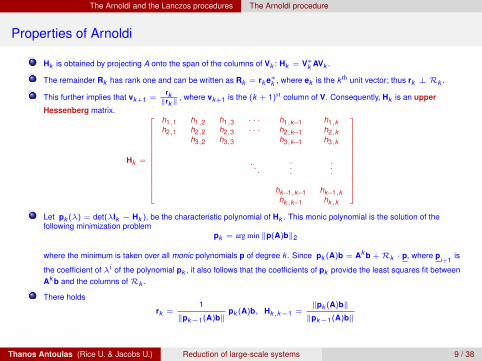
Hk is obtained by projecting A onto the span of the columns of Vk : Hk = V∗k AVk .
The remainder Rk has rank one and can be written as Rk = rk e∗k , where ek is the k th unit vector; thus rk ⊥ Rk .
This further implies that vk+1 =rk‖rk‖
, where vk+1 is the (k + 1)st column of V. Consequently, Hk is an upper
Hessenberg matrix.
Hk =
h1,1 h1,2 h1,3 · · · h1,k−1 h1,kh2,1 h2,2 h2,3 · · · h2,k−1 h2,k
h3,2 h3,3 h3,k−1 h3,k
. . ....
.
.
.
hk−1,k−1 hk−1,khk,k−1 hk,k
Let pk (λ) = det(λIk − Hk ), be the characteristic polynomial of Hk . This monic polynomial is the solution of thefollowing minimization problem
pk = arg min ‖p(A)b‖2
where the minimum is taken over all monic polynomials p of degree k . Since pk (A)b = Ak b +Rk · p, where pi+1
is
the coefficient of λi of the polynomial pk , it also follows that the coefficients of pk provide the least squares fit betweenAk b and the columns ofRk .
There holds
rk =1
‖pk−1(A)b‖pk (A)b, Hk,k−1 =
‖pk (A)b‖‖pk−1(A)b‖
Thanos Antoulas (Rice U. & Jacobs U.) Reduction of large-scale systems 9 / 38
The Arnoldi and the Lanczos procedures The Arnoldi procedure
An alternative way of looking at Arnoldi
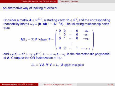
Consider a matrix A ∈ Rn×n, a starting vector b ∈ Rn, and the correspondingreachability matrix Rn = [b Ab · · · An−1b]. The following relationship holdstrue:
ARn = RnF where F =
0 0 · · · 0 −α01 0 · · · 0 −α10 1 · · · 0 −α2
...0 0 · · · 1 −αn−1
and χA(s) = sn + αn−1sn−1 + · · ·+ α1s + α0, is the characteristic polynomialof A. Compute the QR factorization of Rn:
Rn = VU, V∗V = In, U upper triangular
Thanos Antoulas (Rice U. & Jacobs U.) Reduction of large-scale systems 10 / 38
The Arnoldi and the Lanczos procedures The Arnoldi procedure
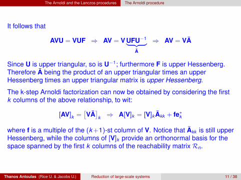
It follows that
AVU = VUF ⇒ AV = V UFU−1︸ ︷︷ ︸A
⇒ AV = VA
Since U is upper triangular, so is U−1; furthermore F is upper Hessenberg.Therefore A being the product of an upper triangular times an upperHessenberg times an upper triangular matrix is upper Hessenberg.
The k-step Arnoldi factorization can now be obtained by considering the firstk columns of the above relationship, to wit:
[AV]k =[VA]
k ⇒ A[V]k = [V]k Akk + fe∗k
where f is a multiple of the (k +1)-st column of V. Notice that Akk is still upperHessenberg, while the columns of [V]k provide an orthonormal basis for thespace spanned by the first k columns of the reachability matrix Rn.
Thanos Antoulas (Rice U. & Jacobs U.) Reduction of large-scale systems 11 / 38
The Arnoldi and the Lanczos procedures The Lanczos procedure
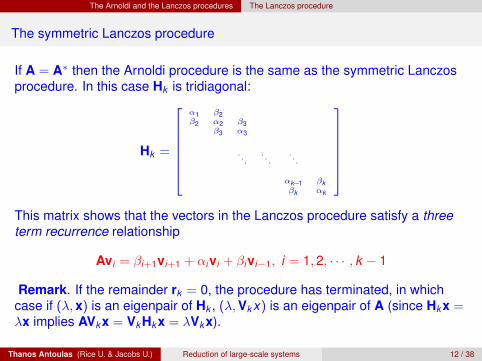
The symmetric Lanczos procedure
If A = A∗ then the Arnoldi procedure is the same as the symmetric Lanczosprocedure. In this case Hk is tridiagonal:
Hk =
α1 β2β2 α2 β3
β3 α3
. . .. . .
. . .
αk−1 βkβk αk
This matrix shows that the vectors in the Lanczos procedure satisfy a threeterm recurrence relationship
Avi = βi+1vi+1 + αivi + βivi−1, i = 1, 2, · · · , k − 1
Remark. If the remainder rk = 0, the procedure has terminated, in whichcase if (λ, x) is an eigenpair of Hk , (λ, Vk x) is an eigenpair of A (since Hk x =λx implies AVk x = Vk Hk x = λVk x).
Thanos Antoulas (Rice U. & Jacobs U.) Reduction of large-scale systems 12 / 38

The Arnoldi and the Lanczos procedures The Lanczos procedure
Two-sided Lanczos
The two-sided Lanczos procedure. Given A ∈ Rn×n which is notsymmetric, and two vectors b, c∗ ∈ Rn, devise a process which is iterativeand the k th step there holds:
AVk = Vk Hk + Rk , A∗Wk = Wk Hk + Sk , k = 1, 2, · · · , n.
Biorthogonality: W∗k Vk = Ik ,
span col Vk = span colRk (A, b), span col Wk = span colRk (A∗, c∗),
Galerkin conditions: V∗k Sk = 0, W∗k Rk = 0, k = 1, 2, · · · , n.
Remarks.
• The second condition of the second item above can also be expressed as span rows W∗k = span rowsOk (c, A), whereOk isthe observability matrix of the pair (c, A).
• The assumption for the solvability of this problem is detOk (c, A)Rk (A, b) 6= 0, k = 1, 2, · · · , n.
• The associated Lanczos polynomials are defined as pk (λ) = det(λIk − Hk ), and the induced inner product is defined as〈p(λ), q(λ)〉 = 〈p(A∗)c∗, q(A)b〉 = c p(A) · q(A) b.
Thanos Antoulas (Rice U. & Jacobs U.) Reduction of large-scale systems 13 / 38
The Arnoldi and the Lanczos procedures The Lanczos procedure
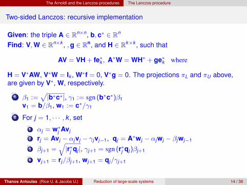
Two-sided Lanczos: recursive implementation
Given: the triple A ∈ Rn×n, b, c∗ ∈ Rn
Find: V, W ∈ Rn×k , , g ∈ Rn, and H ∈ Rk×k , such that
AV = VH + fe∗k , A∗W = WH∗ + ge∗k where
H = V∗AW, V∗W = Ik , W∗f = 0, V∗g = 0. The projections πL and πU above,are given by V∗, W, respectively.
1 β1 :=√|b∗c∗|, γ1 := sgn (b∗c∗)β1
v1 = b/β1, w1 := c∗/γ1
2 For j = 1, · · · , k , set
1 αj = w∗j Avj
2 rj = Avj − αjvj − γjvj−1, qj = A∗wj − αjwj − βjwj−1
3 βj+1 =√|r∗j qj |, γj+1 = sgn (r∗j qj)βj+1
4 vj+1 = rj/βj+1, wj+1 = qj/γj+1
Thanos Antoulas (Rice U. & Jacobs U.) Reduction of large-scale systems 14 / 38

The Arnoldi and the Lanczos procedures The Lanczos procedure
Properties of two-sided Lanczos
Hk is obtained by projecting A as follows: Hk = W∗k AVk .
The remainders Rk , Sk have rank one and can be written as Rk = rk e∗k ,Sk = qk e∗k .
This further implies that vk+1, wk+1 are scaled versions of rk , qkrespectively Consequently, Hk is a tridiagonal matrix.
The generalized Lanczos polynomials pk (λ) = det(λIk − Hk ),k = 0, 1, · · · , n−1, p0 = 1, are orthogonal: 〈pi , pj〉 = 0, for i 6= j .
The columns of Vk , Wk and the Lanczos polynomials satisfy thefollowing three-term recurrences
γk vk+1 = (A− αk )vk − βk−1vk−1βk wk+1 = (A∗ − αk )wk − γk−1wk−1γk pk+1(λ) = (λ− αk )pk (λ) − βk−1pk−1(λ)βk qk+1(λ) = (λ− αk )qk (λ) − γk−1qk−1(λ)
Thanos Antoulas (Rice U. & Jacobs U.) Reduction of large-scale systems 15 / 38
The Arnoldi and the Lanczos procedures An example
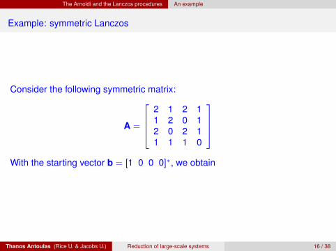
Example: symmetric Lanczos
Consider the following symmetric matrix:
A =
2 1 2 11 2 0 12 0 2 11 1 1 0
With the starting vector b = [1 0 0 0]∗, we obtain
Thanos Antoulas (Rice U. & Jacobs U.) Reduction of large-scale systems 16 / 38

The Arnoldi and the Lanczos procedures An example
V1 =
[ 1000
], H1 = [2], R1 =
[ 0121
]
V2 =
1 00 1√
60 2√
60 1√
6
, H2 =[
2√
6√6 8
3
], R2 =
0 00 1√
540 −1√
540 1√
54
V3 =
1 0 00 1√
61√3
0 2√6
−1√3
0 1√6
1√3
, H3 =
[2
√6 0√
6 83
1√18
0 1√18
43
], R3 =
[0 0 0
0 0√
32
0 0 0
0 0 −√
32
]
V4 =
1 0 0 00 1√
61√3
1√2
0 2√6
−1√3
0
0 1√6
1√3
−1√2
, H4 =
2√
6 0 0√6 8
31√18
0
0 1√18
43
√3√2
0 0√
3√2
0
, R4 = 04×4
where
AVk = Vk Hk + Rk , V∗k Rk = 0 ⇒ Hk = V∗k AVk , k = 1, 2, 3, 4.
Thanos Antoulas (Rice U. & Jacobs U.) Reduction of large-scale systems 17 / 38

Krylov methods and moment matching
Outline
1 Krylov approximation methods
2 The Arnoldi and the Lanczos proceduresThe Arnoldi procedureThe Lanczos procedureAn example
3 Krylov methods and moment matchingRemarks
4 Rational interpolation by Krylov projectionRealization by projectionInterpolation by projection
5 Choice of Krylov projection points: Optimal H2 model reduction
6 Summary: Lectures II and III
Thanos Antoulas (Rice U. & Jacobs U.) Reduction of large-scale systems 18 / 38
Krylov methods and moment matching
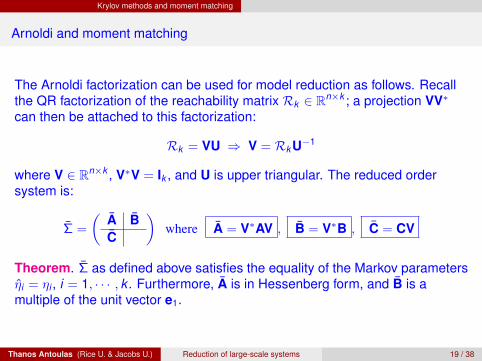
Arnoldi and moment matching
The Arnoldi factorization can be used for model reduction as follows. Recallthe QR factorization of the reachability matrix Rk ∈ Rn×k ; a projection VV∗can then be attached to this factorization:
Rk = VU ⇒ V = Rk U−1
where V ∈ Rn×k , V∗V = Ik , and U is upper triangular. The reduced ordersystem is:
Σ =
(A BC
)where A = V∗AV , B = V∗B , C = CV
Theorem. Σ as defined above satisfies the equality of the Markov parametersηi = ηi , i = 1, · · · , k . Furthermore, A is in Hessenberg form, and B is amultiple of the unit vector e1.
Thanos Antoulas (Rice U. & Jacobs U.) Reduction of large-scale systems 19 / 38

Krylov methods and moment matching
Proof. First notice that since U is upper triangular, v1 = B‖B‖ , and since
V∗Rk = U it follows that B = u1 =‖ B ‖ e1; therefore B = V∗B.VV∗B = VB = B, hence AB = V∗AVV∗B = V∗AB; in general, since VV∗ is aprojection along the columns of Rk , we have VV∗Rk = Rk ; moreover:Rk = V∗Rk ; hence
(η1 · · · ηk ) = CRk = CVV∗Rk = CRk = (η1 · · · ηk )
Finally, the upper triangularity of U implies that A is in Hessenberg form.
Remark.Similarly, one can show that reduction by means the two-sided Lanczosprocedure preserves 2k Markov parameters.
Thanos Antoulas (Rice U. & Jacobs U.) Reduction of large-scale systems 20 / 38
Krylov methods and moment matching Remarks
Remarks
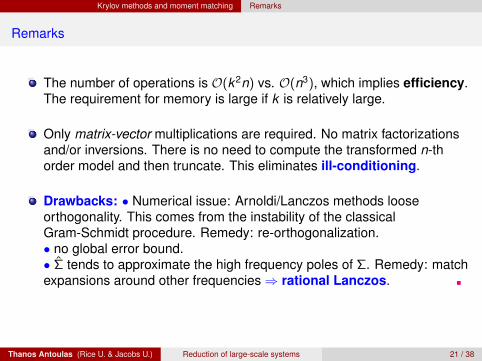
The number of operations is O(k2n) vs. O(n3), which implies efficiency.The requirement for memory is large if k is relatively large.
Only matrix-vector multiplications are required. No matrix factorizationsand/or inversions. There is no need to compute the transformed n-thorder model and then truncate. This eliminates ill-conditioning.
Drawbacks: • Numerical issue: Arnoldi/Lanczos methods looseorthogonality. This comes from the instability of the classicalGram-Schmidt procedure. Remedy: re-orthogonalization.• no global error bound.• Σ tends to approximate the high frequency poles of Σ. Remedy: matchexpansions around other frequencies⇒ rational Lanczos.
Thanos Antoulas (Rice U. & Jacobs U.) Reduction of large-scale systems 21 / 38

Rational interpolation by Krylov projection
Outline
1 Krylov approximation methods
2 The Arnoldi and the Lanczos proceduresThe Arnoldi procedureThe Lanczos procedureAn example
3 Krylov methods and moment matchingRemarks
4 Rational interpolation by Krylov projectionRealization by projectionInterpolation by projection
5 Choice of Krylov projection points: Optimal H2 model reduction
6 Summary: Lectures II and III
Thanos Antoulas (Rice U. & Jacobs U.) Reduction of large-scale systems 22 / 38

Rational interpolation by Krylov projection Realization by projection
Partial realization by projection
Given a system Σ = (A, B, C), where A ∈ Rn×n and B, C∗ ∈ Rn, We seek alower dimensional model Σ = (A, B, C), where A ∈ Rk×k , B, C∗ ∈ Rk , k < n,such that Σ preserves some properties of the original system, throughappropriate projection methods. In other words, we seek V ∈ Rn×k andW ∈ Rn×k such that W∗V = Ik , and the reduced system is given by:A = W∗AV, B = W∗B, C = CV.
Lemma
With V = [B, AB, · · · , Ak−1B] = Rk (A, B) and W any left inverse of V , Σ isa partial realization of Σ and matches k Markov parameters.
From a numerical point of view, one would not use V as defined above since usually the columns of V are almost linearlydependent. As it turns out any matrix whose column span is the same as that of V can be used.
Proof.
We have CB = CVW∗B = CRk (A, B)e1 = CB; furthermore
CAj B = CRk (A, B)W∗AjRk (A, B)e1 = CRk (A, B)W∗Aj B = CRk (A, B)ej+1 = CAj B, j = 1, · · · , k − 1.
Thanos Antoulas (Rice U. & Jacobs U.) Reduction of large-scale systems 23 / 38

Rational interpolation by Krylov projection Interpolation by projection
Rational interpolation by projection
Suppose now that we are given k distinct points sj ∈ C. V is defined as thegeneralized reachability matrix
V =[(s1In − A)−1B, · · · , (sk In − A)−1B
],
and as before, let W be any left inverse of V. Then
Lemma
Σ defined above, interpolates the transfer function of Σ at the sj , that is
H(sj) = C(sj In − A)−1B = C(sj Ik − A)−1B = H(sj), j = 1, · · · , k .
Proof.
The following string of equalities leads to the desired result:
C(sj Ik − A)−1B = CV(sj Ik − W∗AV)−1W∗B
= C[(s1In − A)−1B, · · · , (sk In − A)−1B
] (W∗(sj In − A)V
)−1W∗B
=[C(s1In − A)−1B, · · · , C(sk In − A)−1B
] ([· · · W∗B · · · ]
)−1 W∗B
=[C(s1In − A)−1B, · · · , C(sk In − A)−1B
]ej
= C(sj In − A)−1B.
Thanos Antoulas (Rice U. & Jacobs U.) Reduction of large-scale systems 24 / 38

Rational interpolation by Krylov projection Interpolation by projection
Matching points with multiplicity
We now wish to match the value of the transfer function at a given points0 ∈ C, together with k − 1 derivatives. For this we define the generalizedreachability matrix
V =[(s0In − A)−1B, (s0In − A)−2B, · · · , (s0In − A)−k B
],
together with any left inverse W thereof.
Lemma
Σ interpolates the transfer function of Σ at s0, together with k − 1 derivativesat the same point, j = 0, 1, · · · , k − 1:
(−1)j
j!
d j
dsjH(s)
∣∣∣∣∣s=s0
= C(s0In − A)−(j+1)B = C(s0Ik − A)−(j+1)B =(−1)j
j!
d j
dsjH(s)
∣∣∣∣∣s=s0
Proof.
Let V be as defined as above, and W be such that W∗V = Ik . It readily follows that the projected matrix s0Ir − A is in companionform (expression on the left) and therefore its powers are obtained by shifting its columns to the right:
s0Ik − A = W∗(s0In − A)V = [W∗B, e1, · · · , ek−1] ⇒ (s0Ik − A)` = [ ∗ · · · ∗︸ ︷︷ ︸`−1
, W∗B, e1, · · · , ek−`].
Consequently [W∗(s0In − A)V]−`W∗B = e` , which finally impliesC(s0Ik − A)−`B = CV [W∗(s0I− A)V]−` W∗B = CVe` = C(s0In − A)−`B, ` = 1, 2, · · · , k.
Thanos Antoulas (Rice U. & Jacobs U.) Reduction of large-scale systems 25 / 38

Rational interpolation by Krylov projection Interpolation by projection
General result: rational Krylov
A projector which is composed of any combination of the above three casesachieves matching of an appropriate number of Markov parameters andmoments. Let the partial reachability matrix be
Rk (A, B) =[B AB · · · Ak−1B
],
and partial generalized reachability matrix be:Rk (A, B;σ) =
[(σIn − A)−1B (σIn − A)−2B · · · (σIn − A)−k B
].
Rational Krylov
(a) If V as defined in the above three cases is replaced by V = VR, R ∈ Rk×k ,det R 6= 0, and W by W = R−1W, the same matching results hold true.(b) Let V be such that
span col V = span col [Rk (A, B) Rm1(A, B;σ1) · · · Rm`(A, B;σ`)] ,
and W any left inverse of V. The reduced system matches k Markovparameters and mi moments at σi ∈ C, i = 1, · · · , `.
Thanos Antoulas (Rice U. & Jacobs U.) Reduction of large-scale systems 26 / 38
Rational interpolation by Krylov projection Interpolation by projection
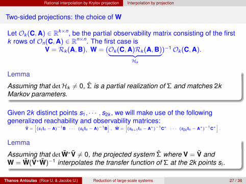
Two-sided projections: the choice of W
Let Ok (C, A) ∈ Rk×n, be the partial observability matrix consisting of the firstk rows of On(C, A) ∈ Rn×n. The first case is
V = Rk (A, B), W = (Ok (C, A)Rk (A, B)︸ ︷︷ ︸Hk
)−1Ok (C, A).
Lemma
Assuming that detHk 6= 0, Σ is a partial realization of Σ and matches 2kMarkov parameters.
Given 2k distinct points s1, · · · , s2k , we will make use of the followinggeneralized reachability and observability matrices:
V =[(s1In − A)−1B · · · (sk In − A)−1B
], W =
[(sk+1In − A∗)−1C∗ · · · (s2k In − A∗)−1C∗
].
Lemma
Assuming that det W∗V 6= 0, the projected system Σ where V = V andW = W(V∗W)−1 interpolates the transfer function of Σ at the 2k points si .
Thanos Antoulas (Rice U. & Jacobs U.) Reduction of large-scale systems 27 / 38
Rational interpolation by Krylov projection Interpolation by projection
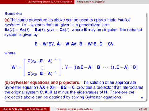
Remarks(a)The same procedure as above can be used to approximate implicitsystems, i.e., systems that are given in a generalized formEx(t) = Ax(t) + Bu(t), y(t) = Cx(t), where E may be singular. The reducedsystem is given by
E = W∗EV, A = W∗AV, B = W∗B, C = CV,
where
W∗ =
C(sk+1E− A)−1
...C(s2k E− A)−1
, V =[(s1E− A)−1B · · · (sk E− A)−1B
](b) Sylvester equations and projectors. The solution of an appropriateSylvester equation AX + XH + BG = 0, provides a projector that interpolatesthe original system C, A, B at minus the eigenvalues of H. Therefore theprojectors above can be obtained by solving Sylvester equations.
Thanos Antoulas (Rice U. & Jacobs U.) Reduction of large-scale systems 28 / 38

Choice of Krylov projection points: OptimalH2 model reduction
Outline
1 Krylov approximation methods
2 The Arnoldi and the Lanczos proceduresThe Arnoldi procedureThe Lanczos procedureAn example
3 Krylov methods and moment matchingRemarks
4 Rational interpolation by Krylov projectionRealization by projectionInterpolation by projection
5 Choice of Krylov projection points: Optimal H2 model reduction
6 Summary: Lectures II and III
Thanos Antoulas (Rice U. & Jacobs U.) Reduction of large-scale systems 29 / 38

Choice of Krylov projection points: OptimalH2 model reduction
Choice of Krylov projection points:Optimal H2 model reduction
Recall: the H2 norm of a stable system is:
‖Σ‖H2 =
(∫ +∞
−∞h2(t)dt
)1/2
where h(t) = CeAtB, t ≥ 0, is the impulse response of Σ.
Goal: construct a Krylov projector such that
Σk = arg mindeg(Σ) = rΣ : stable
∥∥∥Σ− Σ∥∥∥H2
=
(∫ +∞
−∞(h− h)2(t)dt
)1/2
Thanos Antoulas (Rice U. & Jacobs U.) Reduction of large-scale systems 30 / 38
Choice of Krylov projection points: OptimalH2 model reduction
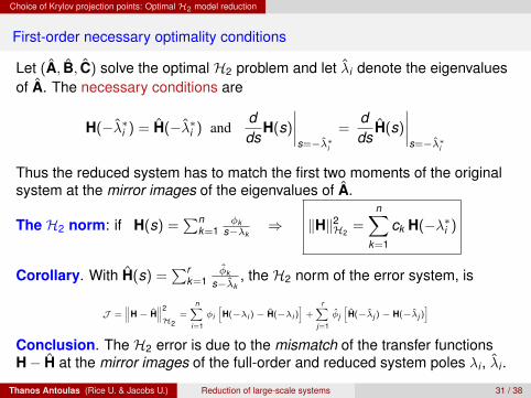
First-order necessary optimality conditions
Let (A, B, C) solve the optimal H2 problem and let λi denote the eigenvaluesof A. The necessary conditions are
H(−λ∗i ) = H(−λ∗i ) anddds
H(s)
∣∣∣∣s=−λ∗i
=dds
H(s)
∣∣∣∣s=−λ∗i
Thus the reduced system has to match the first two moments of the originalsystem at the mirror images of the eigenvalues of A.
The H2 norm: if H(s) =∑n
k=1φk
s−λk⇒ ‖H‖2
H2=
n∑k=1
ck H(−λ∗i )
Corollary. With H(s) =∑r
k=1φk
s−λk, the H2 norm of the error system, is
J =∥∥∥H− H
∥∥∥2
H2=
n∑i=1
φi
[H(−λi )− H(−λi )
]+
r∑j=1
φj
[H(−λj )− H(−λj )
]
Conclusion. The H2 error is due to the mismatch of the transfer functionsH− H at the mirror images of the full-order and reduced system poles λi , λi .
Thanos Antoulas (Rice U. & Jacobs U.) Reduction of large-scale systems 31 / 38

Choice of Krylov projection points: OptimalH2 model reduction
An iterative algorithm
Let the system obtained after the (j − 1)st step be (Cj−1, Aj−1, Bj−1), whereAj−1 ∈ Rk×k , Bj−1, C∗j−1 ∈ Rk . At the j th step the system is obtained as follows
Aj = (W∗j Vj)
−1W∗j AVj , Bj = (W∗
j Vj)−1W∗
j B, Cj = CVj ,
whereVj =
[(λ1I− A)−1B, · · · , (λk I− A)−1B
],
W∗j =
[C(λ1I− A)−1, · · · , C(λk I− A)−1
],
and: −λ1, · · · ,−λk ∈ σ(Aj−1),i.e., −λi are the eigenvalues of the (j − 1)st iterate Aj−1.
The Newton step: can be computed explicitly
λ(k)1
λ(k)2...
←−
λ(k)1
λ(k)2...
− J−1
λ
(k−1)1
λ(k−1)2
.
.
.
⇒ local convergence guaranteed.
Thanos Antoulas (Rice U. & Jacobs U.) Reduction of large-scale systems 32 / 38

Choice of Krylov projection points: OptimalH2 model reduction
An iterative rational Krylov algorithm (IRKA)
The proposed algorithm produces a reduced order model H(s) that satisfiesthe interpolation-based conditions, i.e.
H(−λ∗i ) = H(−λ
∗i ) and
d
dsH(s)
∣∣∣∣s=−λ∗i
=d
dsH(s)
∣∣∣∣s=−λ∗i
1 Make an initial selection of σi , for i = 1, . . . , k
2 W = [(σ1I− A∗)−1C∗, · · · , (σk I− A∗)−1C∗]
3 V = [(σ1I− A)−1B, · · · , (σk I− A)−1B]
4 while (not converged)
A = (W∗V)−1W∗AV,σi ←− −λi(A) + Newton correction, i = 1, . . . , kW = [(σ1I− A∗)−1C∗, · · · , (σk I− A∗)−1C∗]V = [(σ1I− A)−1B, · · · , (σk I− A)−1B]
5 A = (W∗V)−1W∗AV, B = (W∗V)−1W∗B, C = CV
Thanos Antoulas (Rice U. & Jacobs U.) Reduction of large-scale systems 33 / 38

Choice of Krylov projection points: OptimalH2 model reduction
Moderate-dimensional example
total system variables n = 902, independent variables dim = 599, reduceddimension k = 21reduced model captures dominant modes
−2 −1.5 −1 −0.5 0 0.5 1 1.5 2 2.5 3−40
−38
−36
−34
−32
−30
−28
−26
−24
−22
−20
Frequency x 108(rad/s)
Sin
gu
lar
valu
es (
db
)
Frequency responseSpectral zero method with SADPA
n=902 dim=599 k=21
Original
Reduced(SZM)
−0.0136 −0.0135 −0.0135 −0.0134 −0.0134−3
−2
−1
0
1
2
3
Dominant spectral zerosTheoretical and found with SADPA
Real
Imag
Spz: original
Spz: dominant
Spz: SADPA computed
R
C RC
L
C RC
RL
RCC
RLL-
?
- -
??? ?
-
?
. . .
?
u
y
1
Thanos Antoulas (Rice U. & Jacobs U.) Reduction of large-scale systems 34 / 38

Choice of Krylov projection points: OptimalH2 model reduction
H∞ and H2 error norms
Relative norms of the error systems
Reduction Methodn = 902, dim = 599, k = 21 H∞ H2
PRIMA 1.4775 -Spectral Zero Method with SADPA 0.9628 0.841
Optimal H2 0.5943 0.4621Balanced truncation (BT) 0.9393 0.6466
Riccati Balanced Truncation (PRBT) 0.9617 0.8164
Thanos Antoulas (Rice U. & Jacobs U.) Reduction of large-scale systems 35 / 38

Summary: Lectures II and III
Outline
1 Krylov approximation methods
2 The Arnoldi and the Lanczos proceduresThe Arnoldi procedureThe Lanczos procedureAn example
3 Krylov methods and moment matchingRemarks
4 Rational interpolation by Krylov projectionRealization by projectionInterpolation by projection
5 Choice of Krylov projection points: Optimal H2 model reduction
6 Summary: Lectures II and III
Thanos Antoulas (Rice U. & Jacobs U.) Reduction of large-scale systems 36 / 38
Summary: Lectures II and III
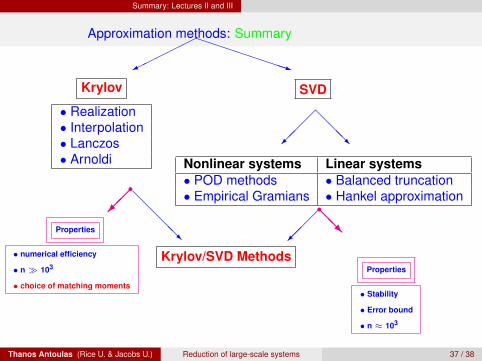
Approximation methods: SummaryPPPPPPPPq
������
Krylov
• Realization• Interpolation• Lanczos• Arnoldi
SVD
@@@R
��
�
Nonlinear systems Linear systems• POD methods • Balanced truncation• Empirical Gramians • Hankel approximation@
@@
@R�
��
Krylov/SVD Methods
��
r@
@R
rProperties
• numerical efficiency
• n� 103
• choice of matching moments
Properties
• Stability
• Error bound
• n ≈ 103
Thanos Antoulas (Rice U. & Jacobs U.) Reduction of large-scale systems 37 / 38
Summary: Lectures II and III
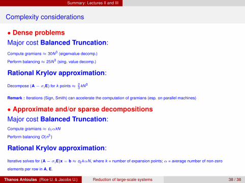
Complexity considerations
• Dense problemsMajor cost Balanced Truncation:Compute gramians≈ 30N3 (eigenvalue decomp.)
Perform balancing≈ 25N3 (sing. value decomp.)
Rational Krylov approximation:
Decompose (A− σi E) for k points≈ 23 kN3
Remark : Iterations (Sign, Smith) can accelerate the computation of gramians (esp. on parallel machines)
• Approximate and/or sparse decompositionsMajor cost Balanced Truncation:Compute gramians≈ c1αkN
Perform balancing O(n3)
Rational Krylov approximation:
Iterative solves for (A− σi E)x = b≈ c2kαN, where k = number of expansion points; α = average number of non-zero
elements per row in A, E.
Thanos Antoulas (Rice U. & Jacobs U.) Reduction of large-scale systems 38 / 38


