model reduction in large scale mimo dynamical systems … · model reduction in large scale mimo...
TRANSCRIPT

“main” — 2008/7/2 — 12:45 — page 211 — #1
Volume 27, N. 2, pp. 211–236, 2008Copyright © 2008 SBMACISSN 0101-8205www.scielo.br/cam
Model reduction in large scale MIMO dynamicalsystems via the block Lanczos method
M. HEYOUNI1, K. JBILOU1, A. MESSAOUDI2 and K. TABAA3
1L.M.P.A, Université du Littoral, 50 rue F. Buisson BP 699, F-62228 Calais Cedex, France2École Normale Supérieure Rabat, Département de Mathématiques, Rabat, Maroc
3Faculté des Sciences Agdal, Département de Mathématiques, Rabat, Maroc
E-mails: [email protected] / [email protected] /
[email protected] / [email protected]
Abstract. In the present paper, we propose a numerical method for solving the coupled
Lyapunov matrix equations
A P + P AT + B BT = 0 and AT Q + Q A + CT C = 0
where A is an n×n real matrix and B, CT are n×s real matrices with rank(B) = rank(C) = s and
s � n. Such equations appear in control problems. The proposed method is a Krylov subspace
method based on the nonsymmetric block Lanczos process. We use this process to produce low
rank approximate solutions to the coupled Lyapunov matrix equations. We give some theoretical
results such as an upper bound for the residual norms and perturbation results. By approximating
the matrix transfer function F(z) = C (z In − A)−1 B of a Linear Time Invariant (LTI) system
of order n by another one Fm(z) = Cm (z Im − Am)−1 Bm of order m, where m is much smaller
than n, we will construct a reduced order model of the original LTI system. We conclude this
work by reporting some numerical experiments to show the numerical behavior of the proposed
method.
Mathematical subject classification: 65F10, 65F30.
Key words: coupled Lyapunov matrix equations; Krylov subspace methods; nonsymmetric
block Lanczos process; reduced order model; transfer functions.
#746/07. Received: 01/VII/07. Accepted: 05/XII/07.

“main” — 2008/7/2 — 12:45 — page 212 — #2
212 MIMO DYNAMICAL SYSTEMS VIA THE BLOCK LANCZOS METHOD
1 Introduction
Consider a stable linear multi-input multi-output (MIMO) state-space model of
the form: {x(t) = A x(t) + B u(t)
y(t) = C x(t),(1.1)
where A ∈ Rn×n , B, CT ∈ Rn×s , x(t) ∈ Rn is the state vector, u(t) ∈ Rs is the
input vector and y(t) ∈ Rs is the output vector of the system (1.1). When dealing
with high-order models, it is reasonable to look for an approximate stable model{
xm(t) = Am xm(t) + Bm u(t)
ym(t) = Cm xm(t),(1.2)
in which Am ∈ Rm×m , Bm, CTm ∈ Rm×s and xm(t), ym(t) ∈ Rm , with m � n.
Hence, the reduction problem consists in approximating the triplet {A, B, C} by
another one { A, B, C} of small size. Several approaches in this area have been
used as Padé approximation [15, 33, 34], balanced truncation [29, 37], optimal
Hankel norm [16, 17] and Krylov subspace methods [3, 6, 11, 12, 21, 22]. These
approaches require the solution of coupled Lyapunov matrix equations [1, 13,
25, 27] having the form{
A P + P AT + B BT = 0
AT Q + Q A + CT C = 0,(1.3)
where P, Q are the controllability and the observability Grammians of the sys-
tem (1.1). For historical developments, applications and importance of Lya-
punov equations and related problems, we refer to [10, 13] and the references
therein. Throughout the paper, we will assume that λi (A) + λ j (A) 6= 0 for all
i, j = 1, . . . , n where λk(A) and it’s conjugate λk(A) are eigenvalues of A. In
this case, the equations (1.3) have unique solutions [26].
Direct methods for solving the Lyapunov matrix equations (1.3) such as those
proposed in [5, 18, 24] are attractive if the matrices are of moderate size. These
methods are based on the Schur or the Hessenberg decomposition. For large
problems, several iterative methods have been proposed; see [14, 22, 23, 32].
These methods use Galerkin projection technics to produce low-dimensional
Sylvester or Lyapunov matrix equations that are solved by using direct methods.
Comp. Appl. Math., Vol. 27, N. 2, 2008

“main” — 2008/7/2 — 12:45 — page 213 — #3
M. HEYOUNI, K. JBILOU, A. MESSAOUDI and K. TABAA 213
For the single-input single-output (SISO) case, i.e., s = 1, two approaches
based on Arnoldi and Lanczos processes were proposed in [21, 22] to solve
large Lyapunov matrix equations. The Arnoldi and Lanczos processes were
also applied in order to give an approximate reduced order model to (1.1) [2, 6,
11, 13].
Our purpose in this paper is to describe a method based on the nonsymmet-
ric block Lanczos process [4, 15, 19, 36] for solving the coupled Lyapunov
matrix equations (1.3). In this method, we project the initial equations onto
block Krylov subspaces generated by the block Lanczos process to produce low-
dimensional Lyapunov matrix equations that are solved by direct methods. By
approximating the transfer function F(z) = C (z In − A)−1 B by another one
Fm(z) = Cm (z Im − Am)−1 Bm where Am ∈ Rm×m , Bm, CTm ∈ Rm×s , and m is
much smaller than n, we will construct an approximate reduced order model of
the continuous time linear system (1.1).
The remainder of the paper is organized as follows. In the following section,
we review the nonsymmetric block Lanczos process and give the exact solutions
of the coupled Lyapunov matrix equations. In Section 3, we first show how to
extract low rank approximate solutions to (1.3). Then, we give some theoretical
results on the residual norms and demonstrate that the low rank approximate
solutions are exact solutions to a pair of perturbed Lyapunov matrix equations.
In Section 4, we consider the problem of obtaining reduced order models to
LTI systems by approximating the associated transfer function. This approach
is based on the nonsymmetric block Lanczos process. Finally, we will present
some numerical experiments.
2 The block Lanczos method and coupled Lyapunov matrix equations
2.1 The nonsymmetric block Lanczos process
Let V ∈ Rn×s and consider the block matrix Krylov subspace Km(A, V ) =
span{V, A V, . . . , Am−1 V }. Notice that Z ∈ Km(A, V ) means that
Z =m−1∑
i=0
Ai V �i , �i ∈ Rs×s, i = 0, . . . m − 1.
Comp. Appl. Math., Vol. 27, N. 2, 2008

“main” — 2008/7/2 — 12:45 — page 214 — #4
214 MIMO DYNAMICAL SYSTEMS VIA THE BLOCK LANCZOS METHOD
We also recall that the minimal polynomial P of A with respect to V is the
nonzero monic polynomial of lowest degree q such that
P(A) ◦ V =q∑
i=0
Ai V �i ,
where �i ∈ Rs×s and �q = Is . The grade of V denoted by grad(V ) is the degree
of the minimal polynomial, hence grad(V ) = q.
In the sequel, we suppose that given two matrices V, W ∈ Rn×s of full rank,
we compute initial block vectors V1 and W1 using the Q R decomposition of
W T V . Hence, if W T V = δ β where δ ∈ Rs×s is an orthogonal matrix (i.e.,
δT δ = δ δT = Is) and β ∈ Rs×s is an upper triangular matrix, then
V1 = V β−1 and W1 = W δ. (2.1)
Given an n × n matrix A and the initial n × s block vectors V , W , the block
Lanczos process applied to the triplet (A, V, W ) and described by Algorithm 1,
generates sequences of n × s right and left block Lanczos vectors {V1, . . . , Vm}
and {W1, . . . , Wm}. These block vectors form biorthonormal bases of the block
Krylov subspaces Km(A, V1) and Km(AT , W1).
Algorithm 1. The nonsymmetric block Lanczos process [4]
• Inputs : A an n × n matrix, V, W two n × s matrices and m an integer.
• Step 0 . Compute the QR decomposition of W T V , i.e., W T V = δ β;
V1 = V β−1; W1 = W δ; V2 = A V1; W2 = AT W1;
• Step 1 . For j = 1, . . . , m
α j = W Tj V j+1; V j+1 = V j+1 − Vj α j ; W j+1 = W j − W j αT
j ;
Compute the QR decompositions of V j+1 and W j+1, i.e.,
V j+1 = Vj+1 β j+1; W j+1 = W j+1 δTj+1;
Compute the singular value decomposition of W Tj+1 Vj+1, i.e.,
W Tj+1 Vj+1 = U j 6 j Z T
j ;
δ j+1 = δ j+1 U j 61/2j ; β j+1 = 6
1/2j V T
j β j+1;
Vj+1 = Vj+1 Z j 6−1/2j ; W j+1 = W j+1 U j 6
−1/2j ;
V j+2 = A Vj+1 − Vj δ j+1; W j+2 = AT W j+1 − W j βTj+1;
end For.
Comp. Appl. Math., Vol. 27, N. 2, 2008
“main” — 2008/7/2 — 12:45 — page 215 — #5
M. HEYOUNI, K. JBILOU, A. MESSAOUDI and K. TABAA 215
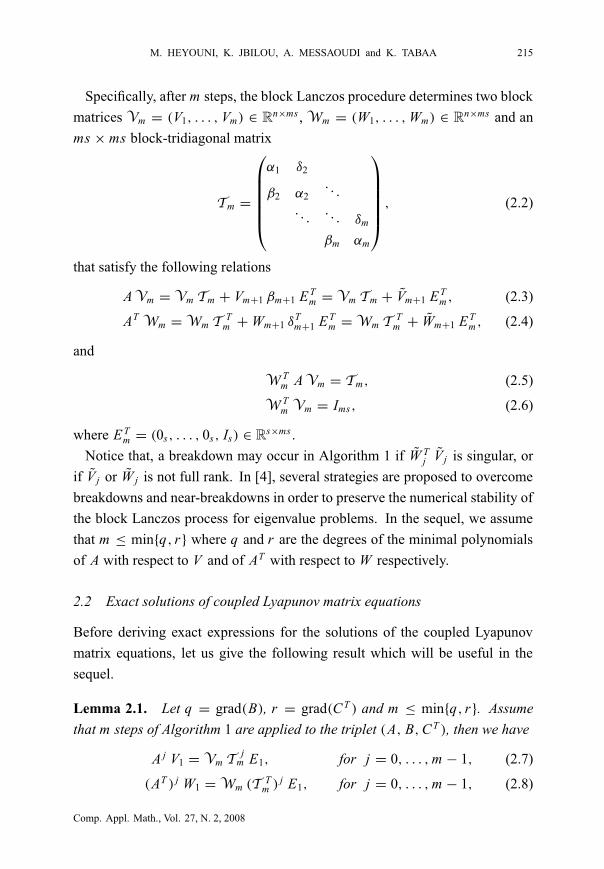
Specifically, after m steps, the block Lanczos procedure determines two block
matrices Vm = (V1, . . . , Vm) ∈ Rn×ms , Wm = (W1, . . . , Wm) ∈ Rn×ms and an
ms × ms block-tridiagonal matrix
Tm =
α1 δ2
β2 α2. . .
. . .. . . δm
βm αm
, (2.2)
that satisfy the following relations
AVm = Vm Tm + Vm+1 βm+1 ETm = Vm Tm + Vm+1 E T
m , (2.3)
AT Wm = Wm TT
m + Wm+1 δTm+1 E T
m = Wm TT
m + Wm+1 E Tm , (2.4)
and
W Tm AVm = Tm, (2.5)
W Tm Vm = Ims, (2.6)
where E Tm = (0s, . . . , 0s, Is) ∈ Rs×ms .
Notice that, a breakdown may occur in Algorithm 1 if W Tj V j is singular, or
if V j or W j is not full rank. In [4], several strategies are proposed to overcome
breakdowns and near-breakdowns in order to preserve the numerical stability of
the block Lanczos process for eigenvalue problems. In the sequel, we assume
that m ≤ min{q, r} where q and r are the degrees of the minimal polynomials
of A with respect to V and of AT with respect to W respectively.
2.2 Exact solutions of coupled Lyapunov matrix equations
Before deriving exact expressions for the solutions of the coupled Lyapunov
matrix equations, let us give the following result which will be useful in the
sequel.
Lemma 2.1. Let q = grad(B), r = grad(CT ) and m ≤ min{q, r}. Assume
that m steps of Algorithm 1 are applied to the triplet (A, B, CT ), then we have
A j V1 = Vm Tj
m E1, for j = 0, . . . , m − 1, (2.7)
(AT ) j W1 = Wm (T Tm ) j E1, for j = 0, . . . , m − 1, (2.8)
Comp. Appl. Math., Vol. 27, N. 2, 2008

“main” — 2008/7/2 — 12:45 — page 216 — #6
216 MIMO DYNAMICAL SYSTEMS VIA THE BLOCK LANCZOS METHOD
where E T1 = (Is, 0s, . . . , 0s) ∈ Rs×ms .
Proof. Since Tm is a block tridiagonal matrix, then for 0 ≤ j ≤ m − 2, T jm is
a block band matrix with j upper-diagonals and j lower-diagonals. Therefore,
letting E Tm = (0s, . . . , 0s, Is) we have
E Tm T
jm E1 = E T
m (T Tm ) j E1 = 0, for j = 0, . . . , m − 2.
Using this last relation and the fact that E Tm E1 = 0, we can proof (2.7) and (2.8)
by induction.
A j+1 V1 = A (A j V1) = A (Vm Tj
m E1)
= (Vm Tm + Vm+1 E Tm)T j
m E1 = Vm Tj+1
m E1.
Using the same arguments, we obtain (2.8). �
Using the previous lemma, we next give the low rank approximate solutions
to (1.3). Let Qq be the minimal polynomial of A with respect to B and q =
grad(B), i.e.,
Qq(A) ◦ B =q∑
i=0
Ai B �i = 0, with �i ∈ Rs×s and �q = Is,
and let Rr be the minimal polynomial of AT for CT where r = grad(CT ), i.e.,
Rr(
AT)◦ CT =
r∑
i=0
(AT
)iCT 9i = 0, with 9i ∈ Rs×s and 9r = Is .
Define
Kq =
0s 0s ∙ ∙ ∙ 0s −�0
Is 0s. . .
... −�1
0s. . .
. . . 0s...
.... . .
. . . 0s...
0s . . . 0s Is −�q−1
and Kr =
0s 0s ∙ ∙ ∙ 0s −90
Is 0s. . .
... −91
0s. . .
. . . 0s...
.... . .
. . . 0s...
0s . . . 0s Is −9r−1
,
as the block companion polynomials of Qq and Rr . Denote by Mq and Nr
the following Krylov matrices
Mq =(B, A B, . . . , Aq−1 B
), Nr =
(CT , AT CT , . . . ,
(AT
)r−1CT
).
Comp. Appl. Math., Vol. 27, N. 2, 2008
“main” — 2008/7/2 — 12:45 — page 217 — #7
M. HEYOUNI, K. JBILOU, A. MESSAOUDI and K. TABAA 217
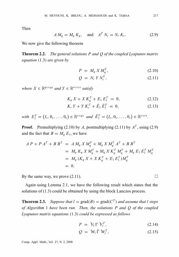
Then
A Mq = Mq Kq, and AT Nr = Nr Kr . (2.9)
We now give the following theorem
Theorem 2.2. The general solutions P and Q of the coupled Lyapunov matrix
equation (1.3) are given by
P = Mq X MTq , (2.10)
Q = Nr Y N Tr , (2.11)
where X ∈ Rqs×qs and Y ∈ Rrs×rs satisfy
Kq X + X K Tq + E1 ET
1 = 0, (2.12)
Kr Y + Y K Tr + E1 E T
1 = 0, (2.13)
with E T1 =
(Is, 0s, . . . , 0s
)∈ Rs×qs and E T
1 =(Is, 0s, . . . , 0s
)∈ Rs×rs .
Proof. Premultiplying (2.10) by A, postmultiplying (2.11) by AT , using (2.9)
and the fact that B = Mq E1, we have
A P + P AT + B BT = A Mq X MTq + Mq X MT
q AT + B BT
= Mq Kq X MTq + Mq X K T
q MTq + Mq E1 E T
1 MTq
= Mq (Kq X + X K Tq + E1 E T
1 )MTq
= 0.
By the same way, we prove (2.11). �
Again using Lemma 2.1, we have the following result which states that the
solutions of (1.3) could be obtained by using the block Lanczos process.
Theorem 2.3. Suppose that l = grad(B) = grad(CT ) and assume that l steps
of Algorithm 1 have been run. Then, the solutions P and Q of the coupled
Lyapunov matrix equations (1.3) could be expressed as follows
P = Vl 0VTl , (2.14)
Q = Wl 0WTl , (2.15)
Comp. Appl. Math., Vol. 27, N. 2, 2008
“main” — 2008/7/2 — 12:45 — page 218 — #8
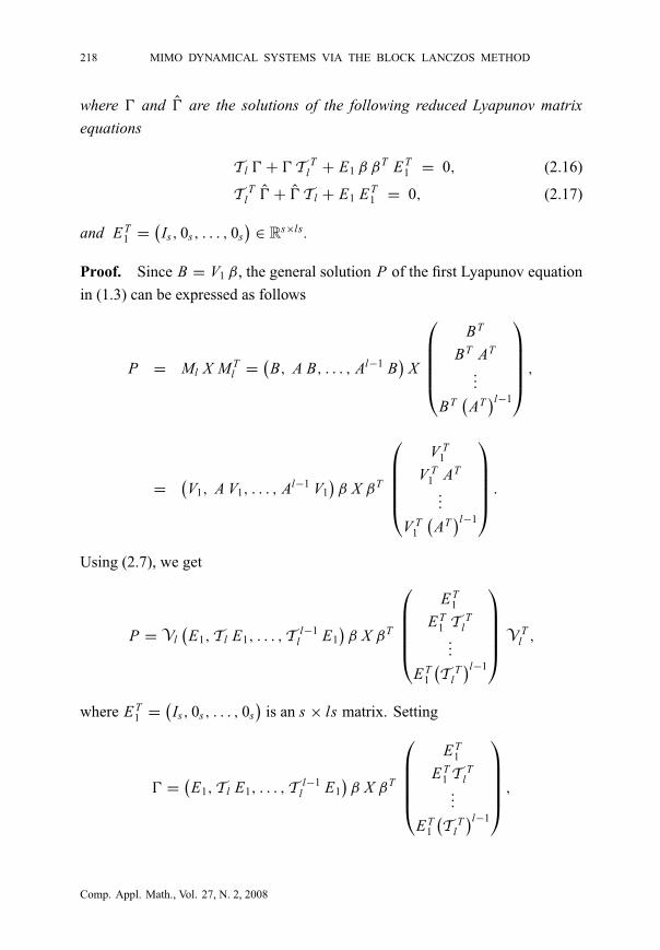
218 MIMO DYNAMICAL SYSTEMS VIA THE BLOCK LANCZOS METHOD
where 0 and 0 are the solutions of the following reduced Lyapunov matrix
equations
Tl 0 + 0T Tl + E1 β βT E T
1 = 0, (2.16)
T Tl 0 + 0Tl + E1 E T
1 = 0, (2.17)
and E T1 =
(Is, 0s, . . . , 0s
)∈ Rs×ls .
Proof. Since B = V1 β, the general solution P of the first Lyapunov equation
in (1.3) can be expressed as follows
P = Ml X MTl =
(B, A B, . . . , Al−1 B
)X
BT
BT AT
...
BT(
AT)l−1
,
=(V1, A V1, . . . , Al−1 V1
)β X βT
V T1
V T1 AT
...
V T1
(AT
)l−1
.
Using (2.7), we get
P = Vl(E1,Tl E1, . . . ,T
l−1l E1
)β X βT
ET1
E T1 T
Tl
...
E T1
(T T
l
)l−1
V T
l ,
where E T1 =
(Is, 0s, . . . , 0s
)is an s × ls matrix. Setting
0 =(E1,Tl E1, . . . ,T
l−1l E1
)β X βT
ET1
E T1 T
Tl
...
E T1
(T T
l
)l−1
,
Comp. Appl. Math., Vol. 27, N. 2, 2008
“main” — 2008/7/2 — 12:45 — page 219 — #9
M. HEYOUNI, K. JBILOU, A. MESSAOUDI and K. TABAA 219
then P = Vl 0VTl and we have
A P + P AT + B BT = AVl 0VTl +Vl 0V
Tl AT + B BT ,
= AVl 0VTl +Vl 0V
Tl AT + V1 β βT V T
1 ,
= 0.
Multiplying the last equalities on the right by Wl , on the left by W Tl and using
(2.5) and (2.6) with m = l we obtain (2.16).
Note that (2.17) is obtained as above by using (2.8), (2.11) and the fact that
CT = W1 δT and δT δ = δ δT = Is . �
Before ending this section, we have to say that in general grad(B) 6= grad(CT ).
Hence, if l = min{grad(B), grad(CT )} and l steps of the nonsymmetric block
Lanczos process have been run, then only (2.14) and (2.16) are satisfied if l =
grad(B). Similarly, only (2.15) and (2.17) are satisfied if l = grad(CT ).
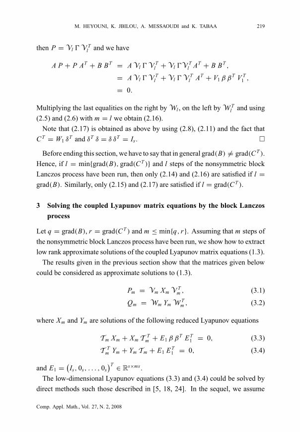
3 Solving the coupled Lyapunov matrix equations by the block Lanczos
process
Let q = grad(B), r = grad(CT ) and m ≤ min{q, r}. Assuming that m steps of
the nonsymmetric block Lanczos process have been run, we show how to extract
low rank approximate solutions of the coupled Lyapunov matrix equations (1.3).
The results given in the previous section show that the matrices given below
could be considered as approximate solutions to (1.3).
Pm = Vm Xm VTm , (3.1)
Qm = Wm Ym WTm , (3.2)
where Xm and Ym are solutions of the following reduced Lyapunov equations
Tm Xm + Xm TT
m + E1 β βT ET1 = 0, (3.3)
T Tm Ym + Ym Tm + E1 E T
1 = 0, (3.4)
and E1 =(Is, 0s, . . . , 0s
)T∈ Rs×ms .
The low-dimensional Lyapunov equations (3.3) and (3.4) could be solved by
direct methods such those described in [5, 18, 24]. In the sequel, we assume
Comp. Appl. Math., Vol. 27, N. 2, 2008

“main” — 2008/7/2 — 12:45 — page 220 — #10
220 MIMO DYNAMICAL SYSTEMS VIA THE BLOCK LANCZOS METHOD
that the eigenvalues λi (Tm) of the block tridiagonal matrix Tm constructed by
the nonsymmetric block Lanczos process satisfy λi (Tm) + λ j (Tm) 6= 0, for
i, j = 1, . . . , m. This condition ensures the existence and uniqueness of Xm and
Ym the solutions of the reduced Lyapunov equations and that these solutions are
symmetric and positive semidefinite.
Next, we show how to compute an upper-bound for the Frobenius residual
norms in order to use it as a stopping criterion. Notice that the upper bound
given below will allow us to stop the algorithm without having to compute the
approximate solutions Pm and Qm . Hence, letting
R(Pm) = A Pm + Pm AT + B BT , (3.5)
R(Qm) = AT Qm + Qm A + CT C, (3.6)
be the residuals associated to Pm and Qm respectively, we have the following
result
Theorem 3.1. Let Pm , Qm be the approximate solutions defined by (3.1), (3.3)
and (3.2), (3.4) respectively. Let R(Pm) and R(Qm) be the corresponding resid-
uals defined by (3.5) and (3.6) respectively. Then
‖R(Pm)‖F ≤ 2 ‖Vm+1 Xm VTm ‖F and
‖R(Qm)‖F ≤ 2 ‖Wm+1 Ym WTm ‖F
(3.7)
where Xm , Ym are the s × n matrices corresponding to the last s rows of Xm and
Ym respectively.
Proof. From (3.1) and (3.3), we have
R(Pm) = AVm XmVTm +Vm XmV
Tm AT + B BT ,
then using (2.3) and the fact that B = V1 β, we get
R(Pm) =(Vm Tm + Vm+1 βm+1 E T
m
)Xm V
Tm
+ Vm Xm(T T
m VTm + Em βT
m+1 V Tm+1
)+ V1 β βT V T
1
= Vm+1
(Tm Xm
βm+1 E Tm Xm
)
V Tm
Comp. Appl. Math., Vol. 27, N. 2, 2008

“main” — 2008/7/2 — 12:45 — page 221 — #11
M. HEYOUNI, K. JBILOU, A. MESSAOUDI and K. TABAA 221
+ Vm
(Xm T T
m Xm Em βTm+1
)V T
m+1 + V1 β βT V T1
= Vm+1
(Tm Xm + Xm T T
m + E1 β βT E T1 Xm Em βT
m+1
βm+1 E Tm Xm 0
)
V Tm+1.
Since Xm is the solution of the reduced Lyapunov equation (3.3) and Vm+1 =
Vm+1 βm+1, then
R(Pm) = Vm+1
(0 Xm Em βT
m+1
βm+1 E Tm Xm 0
)
V Tm+1
= Vm+1 βm+1 E Tm Xm V
Tm +Vm Xm Em βT
m+1 V Tm+1
= Vm+1 E Tm Xm V
Tm +Vm Xm Em V T
m+1.
As Xm is a symmetric matrix, it follows that
‖R(Pm)‖F ≤ 2 ‖Vm+1 E Tm Xm V
Tm ‖F ≤ 2
∥∥∥Vm+1 Xm V
Tm
∥∥∥
F,
where Xm = E Tm Xm represents the s last rows of Xm .
Similarly, from (2.4) and as CT = W1 δT , Wm+1 = Wm+1 δTm+1 and the fact
that Ym is symmetric and is the solution of the reduced Lyapunov equation (3.4),
we obtain the second inequality of (3.7). �
To reduce the cost in the coupled Lyapunov block Lanczos method, the solu-
tion of the low-order Lyapunov equations are computed every k0 iterations where
k0 is a chosen parameter. Note also that the approximate solutions are computed
only when
rm := 2∥∥∥Vm+1 Xm V
Tm
∥∥∥
F≤ ε and sm = 2
∥∥∥Wm+1 Ym W
Tm
∥∥∥
F≤ ε,
where ε is a chosen tolerance. Summarizing the previous results, we get the
following algorithm
Algorithm 2. The coupled Lyapunov block Lanczos algorithm (CLBL)
• Inputs : A an n ×n stable matrix, B an n ×s matrix and C an s ×n matrix.
• Step 0 . Choose a tolerance ε > 0, an integer parameter k0 and set k = 0;
m = k0;
Comp. Appl. Math., Vol. 27, N. 2, 2008

“main” — 2008/7/2 — 12:45 — page 222 — #12
222 MIMO DYNAMICAL SYSTEMS VIA THE BLOCK LANCZOS METHOD
• Step 1 . For j = k + 1, k + 2, . . . , m;
construct the block tridiagonal matrix Tm , the biorthonormal
bases {Vk+1, . . . , Vm}, {Wk+1, . . . , Wm}, Vm+1 and Wm+1 by
Algorithm 1 applied to the triplet (A, B, CT );
end For
• Step 2 . Solve the low-dimensional Lyapunov equations:
Tm Xm + Xm TT
m + E1 β βT E T1 = 0;
T Tm Ym + Ym Tm + E1 E T
1 = 0;
• Step 3 . Compute the upper bounds for the residual norms:
rm = 2∥∥∥Vm+1 Xm V
Tm
∥∥∥
Fand sm = 2
∥∥∥Wm+1 Ym W
Tm
∥∥∥
F;
• Step 4 . If rm > ε or sm > ε, set k = k + k0; m = k + k0 and go to step 1.
• Step 5 . The approximate solutions are represented by the matrix product:
Pm = Vm Xm VTm and Qm = Wm Ym W
Tm .
We end this section by the following result which shows that the approximate
solutions Pm and Qm are the exact solutions of two perturbed Lyapunov matrix
equations.
Theorem 3.2. Suppose that m steps of Algorithm 2 have been run. Let Pm ,
Qm be the approximate solutions defined by (3.1), (3.3) and (3.2), (3.4) re-
spectively. Then Pm and Qm are the exact solutions of the perturbed Lyapunov
matrix equations
(A − 11) Pm + Pm(A − 11)T + B BT = 0, (3.8)
(A − 12)T Qm + Qm (A − 12) + CT C = 0, (3.9)
where
11 = Vm+1 W Tm and 12 = Vm W T
m+1. (3.10)
Comp. Appl. Math., Vol. 27, N. 2, 2008
“main” — 2008/7/2 — 12:45 — page 223 — #13
M. HEYOUNI, K. JBILOU, A. MESSAOUDI and K. TABAA 223
Proof. Multiplying (3.3) on the left by Vm , on the right by V Tm , we obtain
Vm Tm Xm VTm +Vm Xm T T
m VTm +Vm E1 β βT E T
1 VTm = 0.
Using (2.3), we have
[AVm − Vm+1 βm+1 E T
m
]Xm V
Tm
+Vm Xm[V T
m AT − Em βTm+1 V T
m+1
]+ B BT = 0,
and since W Tm Vm = Ims , then
[A − Vm+1 βm+1 E T
m WTm
]Vm Xm V
Tm
+Vm Xm VTm
[AT −Wm Em βT
m+1 V Tm+1
]+ B BT = 0.
Hence,
(A − 11
)Pm + Pm
(A − 11
)T+ B BT = 0,
where
11 = Vm+1 βm+1 E Tm W
Tm = Vm+1 βm+1 W T
m = Vm+1 W Tm .
We use the same arguments to show (3.9). �
4 Reduced order models via the nonsymmetric block Lanczos process
In this section, we consider the following state formulation of a multi-input and
multi-output linear time invariant system (LTI){
x(t) = A x(t) + B u(t)
y(t) = C x(t),(4.1)
where x(t) ∈ Rn is the state vector, u(t) ∈ Rs is the input, y(t) ∈ Rs is the out-
put of interest and A ∈ Rn×n, B, CT ∈ Rn×s . Applying the Laplace transform
to (4.1), we obtain{
z X (z) = A X (z) + B U (z)
Y (z) = C X (z),
Comp. Appl. Math., Vol. 27, N. 2, 2008
“main” — 2008/7/2 — 12:45 — page 224 — #14
224 MIMO DYNAMICAL SYSTEMS VIA THE BLOCK LANCZOS METHOD
where X (z), Y (z) and U (z) are the Laplace transforms of x(t), y(t) and u(t)
respectively.
The standard way of relating the input and output vectors of (4.1) is to use
the associated transfer function F(z) such that Y (z) = F(z) U (z). Hence, if we
eliminate X (z) in the previous two equations, we get:
F(z) = C(z In − A
)−1B. (4.2)
We recall that most of model reduction techniques, like the moment-matching
approaches, are based on this transfer function [2, 13, 15, 20, 22]. Moreover,
if the number of state variables of the previous LTI system is very high, (i.e., if
n the order of A is large), direct computations of F(z) becomes inefficient or
even prohibitive. Hence, it is reasonable to look for a model of low order that
approximates the behavior of the original model (4.1). This low-order model
can be expressed as follows{
xm(t) = Am xm(t) + Bm u(t)
ym(t) = Cm xm(t),(4.3)
where Am ∈ Rm×m , Bm and CTm ∈ Rm×s with m � n.
In [22] and for the single-input single-output case (i.e., s = 1), the authors
proposed a method based on the classical Lanczos process to construct an ap-
proximate reduced order model to (4.1). The aim of this section is to generalize
some of the results given in [22] to the multi-input multi-output case.
More precisely, let us see how to obtain an efficient reduced model to (4.1) by
using the nonsymmetric block Lanczos process. This is done by computing an
approximate transfer function Fm(z) to the original one F(z). In fact, writing
F(z) = C X where X = (z In − A)−1 B ∈ Rn×s and considering the block
linear system(z In − A
)X = B, (4.4)
we see that, approximating F(z) can be achieved by computing an approximate
solution Xm to X by using the block Lanczos method for solving linear systems
with multiple right-hand sides [19].
LettingVm ,Wm and Tm be the biorthonormal bases and the block tridiagonal
matrix, respectively, given by the nonsymmetric block Lanczos process applied
Comp. Appl. Math., Vol. 27, N. 2, 2008

“main” — 2008/7/2 — 12:45 — page 225 — #15
M. HEYOUNI, K. JBILOU, A. MESSAOUDI and K. TABAA 225
to the triplet (A, B, CT ) and starting from an initial guess X0 = 0, we can show
that
Xm = Vm(z Ims − Tm
)−1E1 β.
Since
C = δ W T1 and W T
1 Vm =(Is, 0, . . . , 0
)T= E T
1 ∈ Rs×ms,
the transfer function F(z) can then be approximated by
Fm(z) = C Xm = δ E T1
(z Ims − Tm
)−1E1 β. (4.5)
The above result allows us to suggest the following reduced order model to (4.1){
xm(t) = Tm xm(t) + E1 β u(t)
ym(t) = δ E T1 xm(t),
(4.6)
Next, we show that the reduced order model (4.5) proposed in the above ap-
proach approximates the behavior of the original model (4.1). Moreover, we give
an upper bound for ‖Fm(z) − F(z)‖ which enable us to monitor the progress of
the iterative process at each step. More precisely, we have the following results
Theorem 4.1. The matrices Tm , β and δ generated by the block Lanczos pro-
cess applied to the triplet (A, B, CT ) are such that the first 2m − 1 Markov
parameters of the original and the reduced models are the same, that is,
C A j B =(δ E T
1
)T k
m
(E1 β
)for j = 0, 1, . . . , 2(m − 1).
Proof. For j ∈ {0, 1, . . . , 2m − 1}, let j1, j2 ∈ {0, 1, . . . , m − 1} such that
j = j1 + j2. Using the results of Lemma 2.1 and the fact that C = δ W T1 ,
W T1 Vm = E T
1 , we have
C A j B = δ W T1 A j1+ j2 V1 β = δ
[(AT ) j2 W1
]T [A j1 V1
]β
= δ[Wm (T T
m ) j2 E1]T [
Vm Tj1
m E1]
β
= δ E T1 T
j2m
[W T
m Vm]T j1
m E1 β = δ E T1 T
j1+ j2m E1 β
= (δ E T1 )T j
m (E1 β).
�
Before giving an upper bound for ‖Fm(z) − F(z)‖, we have to recall the
definition of the Schur complement [35] and give the first matrix Sylvester iden-
tity [28].
Comp. Appl. Math., Vol. 27, N. 2, 2008

“main” — 2008/7/2 — 12:45 — page 226 — #16
226 MIMO DYNAMICAL SYSTEMS VIA THE BLOCK LANCZOS METHOD
Definition 4.2. Let M be a matrix partitioned into four blocks
M =
(A B
C D
)
,
where the submatrix D is assumed to be square and nonsingular. The Schur
complement of D in M, denoted by (M/D), is defined by
(M/D) = A− BD−1C.
If D is not a square matrix then a pseudo-Schur complement of D in M can
still be defined [7, 8]. Now, considering the matrices K and M partitioned as
follows
K =
A B E
C D F
G H L
M =
(D F
H L
)
,
we have the following property
Proposition 4.3. If the matrices L and M are square and nonsingular, then
(K/M
)=
((K/L)/(M/L)
)=
((A E
G L
)
/L
)
−
((B E
H L
)
/L
)(M/L
)−1
((C F
G L
)
/L
)
.
Theorem 4.4. Let αi , β, βi , δ, δi (1 ≤ i ≤ m), Vm+1 and Wm+1 be the matrices
obtained after m steps of the nonsymmetric block Lanczos process applied to
the triplet (A, B, CT ). If (z Ims − Tm), (z In − A) are nonsingular and z is such
that |z| > ‖A‖2, then
‖F(z) − Fm(z)‖2 ≤‖δ‖2 ‖01,m(z)‖2 ‖Wm+1‖2 ‖Vm+1‖2 ‖0m,1(z)‖2 ‖β‖2
|z| − ‖A‖2, (4.7)
where0m,1(z) = E T
m (z Ims − Tm)−1 E1
= Dm βm Dm−1 βm−1 ∙ ∙ ∙ D2 β2 D1,(4.8)
Comp. Appl. Math., Vol. 27, N. 2, 2008
“main” — 2008/7/2 — 12:45 — page 227 — #17
M. HEYOUNI, K. JBILOU, A. MESSAOUDI and K. TABAA 227
01,m(z) = E T1 (z Ims − Tm)−1 Em
= D1 δ2 D2 ∙ ∙ ∙ δm−1 Dm−1 δm Dm,(4.9)
and
Dm = (z Is − αm)−1, D j−1 = (z Is − α j−1 − δ j D j β j )−1 for j = m, . . . , 2.
Proof. As C = δ W T1 and B = V1 β, we have
F(z) − Fm(z) = C (z In − A)−1 B − δ E T1 (z Ims − Tm)−1 E1 β
= δ W T1 (z In − A)−1 V1 β − δ ET
1 (z Ims − Tm)−1 E1 β
= δ G(z) β,
where G(z) = W T1 (z In − A)−1 V1 − E T
1 (z Ims − Tm)−1 E1. Now, from (2.3),
we have
Vm (z Ims − Tm)−1 = (z In − A)−1(z In − A)Vm (z Ims − Tm)−1
= (z In − A)−1 (zVm − AVm) (z Ims − Tm)−1
= (z In − A)−1 (zVm −Vm Tm − Vm+1 ETm) (z Ims − Tm)−1
= (z In − A)−1Vm − (z In − A)−1 Vm+1 ETm (z Ims − Tm)−1.
Multiplying the last relation on the left by W T1 , on the right by E1 we obtain
G(z) = W T1 (z In − A)−1 Vm+1 E T
m (z Ims − Tm)−1 E1. (4.10)
Similarly, by using (2.4), we have
(z Ims − Tm)−1W Tm = (z Ims − Tm)−1W T
m (z In − A) (z In − A)−1
= (z Ims − Tm)−1 (zW Tm −W T
m A)(z In − A)−1
= (z Ims − Tm)−1(zW Tm − Tm W
Tm − Em W T
m+1) (z In − A)−1
= (W Tm (z In − A)−1 − (z Ims − Tm)−1 Em W T
m+1 (z In − A)−1
and again, multiplying the last equality on the left by E T1 , on the right by Vm+1,
we have
W T1 (z In − A)−1 Vm+1 − ET
1 (z Ims − Tm)−1 Em W Tm+1 (z In − A)−1 Vm+1 = 0. (4.11)
Comp. Appl. Math., Vol. 27, N. 2, 2008

“main” — 2008/7/2 — 12:45 — page 228 — #18
228 MIMO DYNAMICAL SYSTEMS VIA THE BLOCK LANCZOS METHOD
Combining the formulas (4.10), (4.11) and letting
0m,1(z) = E Tm (z Ims − Tm)−1 E1, 01,m(z) = E T
1 (z Ims − Tm)−1 Em,
we get
G(z) = 01,m(z) W Tm+1 (z In − A)−1 Vm+1 0m,1(z),
and then
F(z) − Fm(z) = δ[01,m(z) W T
m+1 (z In − A)−1 Vm+1 0m,1(z)]
β.
Finally, using the inequality ‖(z In − A)−1‖2 ≤ 1|z|−‖A‖2
for |z| > ‖A‖2, we have
‖F(z) − Fm(z)‖2
≤ ‖δ‖2 ‖01,m(z)‖2 ‖Wm+1‖2 ‖(z In − A)−1‖2 ‖Vm+1‖2 ‖0m,1(z)‖2 ‖β‖2
≤‖δ‖2 ‖01,m(z)‖2 |Wm+1‖2 ‖Vm+1‖2 |0m,1(z)‖2 ‖β‖2
|z| − ‖A‖2.
Next, set Dm = (z Is − αm)−1 and remark that 0m,1(z) is the Schur comple-
ment of
(z Ims − Tm) in
(0 −E T
m
E1 z Ims − Tm
)
.
Hence, using the result of Proposition 4.3, we have
0m,1(z) =
((0 −E T
m
E1 z Ims − Tm
)
/(z Ims − Tm)
)
=
0 0 −Is
E1 z I(m−1)s − Tm−1 −δm Em−1
0 −βm E Tm−1 z Is − αm
/(z Ims − Tm)
=
((0 −Is
0 D−1m
)
/D−1m
)
−
((0 −Is
−βm E Tm−1 D−1
m
)
/D−1m
)
×
((z I(m−1)s − Tm−1 −δm Em−1
−βm E Tm−1 D−1
m
)
/D−1m
)−1
×
((E1 −δm Em−1
0 D−1m
)
/D−1m
)
= Dm βm E Tm−1
[z I(m−1)s − Tm−1 − δm Em−1 Dm βm E T
m−1
]−1E1
= Dm βm E Tm−1 (z I(m−1)s − Tm−1)
−1 E1,
Comp. Appl. Math., Vol. 27, N. 2, 2008

“main” — 2008/7/2 — 12:45 — page 229 — #19
M. HEYOUNI, K. JBILOU, A. MESSAOUDI and K. TABAA 229
where
E T1 =
(Is, 0s, ∙ ∙ ∙ , 0s
)∈ Rs×(m−1)s, E T
m−1 =(0s, ∙ ∙ ∙ , 0s, Is
)∈ Rs×(m−1)s
and Tm−1 is a block tridiagonal matrix having the same elements that Tm−1
except the (m − 1, m − 1) block which is equal to (αm−1 + δm Dm βm).
Again, applying Proposition 4.3 to compute E Tm−1 (z I(m−1)s − Tm−1)
−1 E1,
and so on, we finally obtain (4.8). Similarly, we remark that 01,m(z)T is the
Schur complement of
(z Ims − T T
m
)in
(0 −E T
m
E1 z Ims − T Tm
)
.
Then, using the same arguments as for 0m,1(z) we get (4.9). �
Summarizing the previous results, we get the following algorithm
Algorithm 4. Model reduction via the block Lanczos process
• Inputs : A the system matrix, B the input matrix, C the output matrix.
• Step 0 . Choose a tolerance ε > 0, an integer parameter k0 and set k = 0;
m = k0.
• Step 1 . For j = k + 1, k + 2, . . . , m
construct the block tridiagonal matrix Tm , Vm+1 and Wm+1 by
Algorithm 1 applied to the triplet (A, B, CT ).
compute the matrices 01,m(z) and 0m,1(z) using (4.8), (4.9).
end For
• Step 2 . Compute the upper bound for the residual norm:
rm =‖δ‖2 ‖01,m(z)‖2 ‖Wm+1‖2 ‖Vm+1‖2 ‖0m,1(z)‖2 ‖β‖2
|z| − ‖A‖2.
• Step 3 . If rm > ε, set k = k + k0; m = k + k0 and go to step 1.
• Step 4 . The reduced order model is Am = Tm , Bm = E1 β and Cm =
δ E T1 .
Comp. Appl. Math., Vol. 27, N. 2, 2008
“main” — 2008/7/2 — 12:45 — page 230 — #20
230 MIMO DYNAMICAL SYSTEMS VIA THE BLOCK LANCZOS METHOD
5 Numerical experiments
In this section, we present some numerical experiments to illustrate the behavior
of the block Lanczos process when applied to solve coupled Lyapunov equations.
We also applied the block Lanczos process for model reduction in large scale
dynamical systems. All the experiments were performed on a computer of Intel
Pentium-4 processor at 3.4GHz and 1024 MBytes of RAM. The experiments
were done using Matlab 6.5.
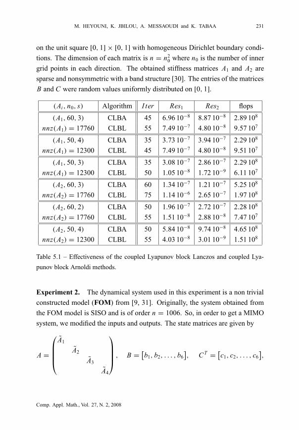
Experiment 1. In this first experiment, we compared the performance of the
coupled Lyapunov block Lanczos (CLBL) and the coupled Lyapunov block
Arnoldi (CLBA) algorithms [21]. Notice that:
• In all the experiments, the parameter k0 used to compute the solutions of
the low-order Lyapunov equations is k0 = 5.
• For the coupled Lyapunov block Arnoldi algorithm, the tests were stopped
when the residual given in [21] was less than ε = 10−6.
• For the coupled Lyapunov block Lanczos algorithm, the iterations were
stopped when
max{‖Vm+1 Xm‖F , ‖Wm+1 Ym‖F
}≤ ε = 10−6. (5.1)
We note that Res1 =‖ A Pm + Pm AT + B BT ‖F and Res2 =‖ AT Qm +
Qm A + CT C ‖F are the exact Frobenius residual norms for the first and the
second Lyapunov equations (1.3) respectively. The number I ter of iterations
required for CLBA corresponds to the total number of iterations needed for
solving separately the two Lyapunov equations (1.3) by the Lyapunov block
Arnoldi method.
The matrices A1 and A2 tested in this experiment comes from the five-point
discretization of the operators [30]
L1(u) = 1u − (x − y)∂u
∂x− sin (x + y)
∂u
∂y− 103 ex y u,
L2(u) = 1u −1
2
√x + y
∂u
∂x− (cos(x) + cos(y))
∂u
∂y− (x + y) u,
Comp. Appl. Math., Vol. 27, N. 2, 2008
“main” — 2008/7/2 — 12:45 — page 231 — #21
M. HEYOUNI, K. JBILOU, A. MESSAOUDI and K. TABAA 231
on the unit square [0, 1] × [0, 1] with homogeneous Dirichlet boundary condi-
tions. The dimension of each matrix is n = n20 where n0 is the number of inner
grid points in each direction. The obtained stiffness matrices A1 and A2 are
sparse and nonsymmetric with a band structure [30]. The entries of the matrices
B and C were random values uniformly distributed on [0, 1].
(Ai , n0, s) Algorithm I ter Res1 Res2 flops
(A1, 60, 3) CLBA 45 6.96 10−8 8.87 10−8 2.89 108
nnz(A1) = 17760 CLBL 55 7.49 10−7 4.80 10−8 9.57 107
(A1, 50, 4) CLBA 35 3.73 10−7 3.94 10−7 2.29 108
nnz(A1) = 12300 CLBL 45 7.49 10−7 4.80 10−8 9.51 107
(A1, 50, 3) CLBA 35 3.08 10−7 2.86 10−7 2.29 108
nnz(A1) = 12300 CLBL 50 1.05 10−8 1.72 10−9 6.11 107
(A2, 60, 3) CLBA 60 1.34 10−7 1.21 10−7 5.25 108
nnz(A2) = 17760 CLBL 75 1.14 10−6 2.65 10−7 1.97 108
(A2, 60, 2) CLBA 50 1.96 10−7 2.72 10−7 2.28 108
nnz(A2) = 17760 CLBL 55 1.51 10−8 2.88 10−8 7.47 107
(A2, 50, 4) CLBA 50 5.84 10−8 9.74 10−8 4.65 108
nnz(A2) = 12300 CLBL 55 4.03 10−8 3.01 10−9 1.51 108
Table 5.1 – Effectiveness of the coupled Lyapunov block Lanczos and coupled Lya-
punov block Arnoldi methods.
Experiment 2. The dynamical system used in this experiment is a non trivial
constructed model (FOM) from [9, 31]. Originally, the system obtained from
the FOM model is SISO and is of order n = 1006. So, in order to get a MIMO
system, we modified the inputs and outputs. The state matrices are given by
A =
A1
A2
A3
A4
, B =[b1, b2, . . . , b6
], CT =
[c1, c2, . . . , c6
],
Comp. Appl. Math., Vol. 27, N. 2, 2008

“main” — 2008/7/2 — 12:45 — page 232 — #22
232 MIMO DYNAMICAL SYSTEMS VIA THE BLOCK LANCZOS METHOD
where
A1 =
(−1 100
−100 −1
)
, A2 =
(−1 200
−200 −1
)
, A3 =
(−1 400
−400 −1
)
and A4 = diag(−1, . . . , −1000). The columns of B and C are such that
bT1 = c1 = (10, . . . , 10︸ ︷︷ ︸
6
, 1, . . . , 1︸ ︷︷ ︸1000
), and b2, . . . , b6; c2, . . . , c6
are random column vectors.
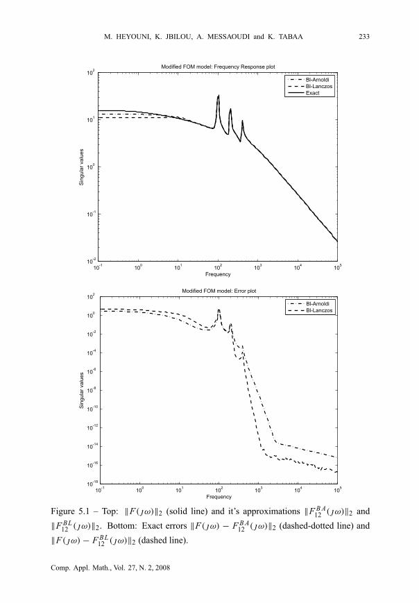
The response plot and error plot given below show the singular values
σmax(F( ω)) and σmax(Fm( ω) − F( ω)) as a function of the frequency ω re-
spectively, where σmax(.) denotes the largest singular value and ω ∈ [10−1 105].
As a stopping criterion, we used the upper bound (4.7). More precisely, we
stopped the computation when
maxw
(‖δ‖2 ‖01,m(z)‖2 ‖Wm+1‖2 ‖Vm+1‖2 ‖0m,1(z)‖2 ‖β‖2
|z| − ‖A‖2
)
≤ η = 10−7.
The frequency response (solid line) of the modified FOM model is given in the
top of Figure 5.1 and is compared to the frequencies responses of order m = 12
when using the block Arnoldi process (dash-dotted line) and the block Lanczos
process (dashed line). The exact errors ‖F(z) − F12(z)‖2 produced by the two
processes are shown in the bottom of Figure 5.1.
6 Conclusion
In this paper, we applied the block Lanczos process for solving coupled Lya-
punov matrix equations and also for model reduction. We gave some new theo-
retical results and showed the effectiveness of this process with some numerical
examples.
Acknowledgments. We would like to thank the referees for their recommen-
dations and helpful suggestions.
Comp. Appl. Math., Vol. 27, N. 2, 2008
“main” — 2008/7/2 — 12:45 — page 233 — #23
M. HEYOUNI, K. JBILOU, A. MESSAOUDI and K. TABAA 233
10-1
100
101
102
103
104
105
10-2
10-1
100
101
102
Frequency
Sin
gula
r va
lues
Modified FOM model: Frequency Response plot
Bl-ArnoldiBl-LanczosExact
10-1
100
101
102
103
104
105
10-18
10-16
10-14
10-12
10-10
10-8
10-6
10-4
10-2
100
102
Frequency
Sin
gula
r va
lues
Modified FOM model: Error plot
Bl-ArnoldiBl-Lanczos
Figure 5.1 – Top: ‖F(ω)‖2 (solid line) and it’s approximations ‖F B A12 (ω)‖2 and
‖F BL12 (ω)‖2. Bottom: Exact errors ‖F(ω) − F B A
12 (ω)‖2 (dashed-dotted line) and
‖F(ω) − F BL12 (ω)‖2 (dashed line).
Comp. Appl. Math., Vol. 27, N. 2, 2008

“main” — 2008/7/2 — 12:45 — page 234 — #24
234 MIMO DYNAMICAL SYSTEMS VIA THE BLOCK LANCZOS METHOD
REFERENCES
[1] A.C. Antoulas and D.C. Sorensen, Projection methods for balanced model reduction, Technical
Report, Rice University, Houston, Tx, (2001).
[2] Z. Bai and Q. Ye, Error estimation of the Padé approximation of transfer functions via the
Lanczos process. Elect. Trans. Numer. Anal., 7 (1998), 1–17.
[3] Z. Bai, Krylov subspace techniques for reduced-order modeling of large-scale dynamical
systems. App. Num. Math., 43 (2002), 9–44.
[4] Z. Bai, D. Day and Q. Ye, ABLE: An adaptive block Lanczos method for non-Hermitian
eigenvalue problems. SIAM J. Mat. Anal. Appl., 20(4) (1999), 1060–1082.
[5] R.H. Bartels and G.W. Stewart, Solution of the matrix equation AX + X B = C . Comm.
ACM, 15 (1972), 820–826.
[6] D.L. Boley and B.N. Datta, Numerical methods for linear control systems, in: C. Byrnes,
B. Datta, D. Gilliam, C. Martin (Eds.) Systems and Control in the twenty-First Century,
Birkhauser, pp. 51–74, (1996).
[7] C. Brezinski and M.R. Zaglia, A Schur complement approach to a general extrapolation
algorithm. Linear Algebra Appl., 368 (2003), 279–301.
[8] D. Carlson, What are Schur complements, anyway? Linear Algebra Appl., 74 (1986),
257–275.
[9] Y. Chahlaoui and P. Van Dooren, A collection on Benchmark examples for model reduction
of linear time invariant dynamical systems. SILICOT Working Note 2002-2.
http://www.win.tue.nl/niconet/NIC2/benchmodred.html.
[10] B.N. Datta, Linear and numerical linear algebra in control theory: Some research problems.
Lin. Alg. Appl., 197-198 (1994), 755–790.
[11] B.N. Datta, Large-Scale Matrix computations in Control. Applied Numerical Mathematics,
30 (1999), 53–63.
[12] B.N. Datta, Krylov Subspace Methods for Large-Scale Matrix Problems in Control. Future
Gener. Comput. Syst., 19(7) (2003), 1253–1263.
[13] B.N. Datta, Numerical Methods for Linear Control Systems Design and Analysis. Elsevier
Academic Press, (2003).
[14] A. El Guennouni, K. Jbilou and A.J. Riquet, Block Krylov subspace methods for solving
large Sylvester equations. Numer. Alg., 29 (2002), 75–96.
[15] P. Feldmann and R.W. Freund, Efficient Linear Circuit Analysis by Padé Approximation via
The Lanczos process. IEEE Trans. on CAD of Integrated Circuits and Systems, 14 (1995),
639–649.
[16] K. Glover, All optimal Hankel-norm approximations of linear multivariable systems and
their L-infinity error bounds. International Journal of Control, 39 (1984), 1115–1193.
Comp. Appl. Math., Vol. 27, N. 2, 2008

“main” — 2008/7/2 — 12:45 — page 235 — #25
M. HEYOUNI, K. JBILOU, A. MESSAOUDI and K. TABAA 235
[17] K. Glover, D.J.N. Limebeer, J.C. Doyle, E.M. Kasenally and M.G. Safonov, A characteri-
sation of all solutions to the four block general distance problem. SIAM J. Control Optim.,
29 (1991), 283–324.
[18] G.H. Golub, S. Nash and C. Van Loan, A Hessenberg-Schur method for the problem A X +
X B = C . IEEE Trans. Autom. Control, AC-24 (1979), 909–913.
[19] G.H. Golub and R. Underwood, The block Lanczos method for computing eigenvalues.
Mathematical Software III, J.R. Rice, ed., Academic Press, New York, pp. 361–377, (1977).
[20] E.J. Grimme, D.C. Sorensen and P. Van Dooren, Model reduction of state space systems via
an implicitly restarted Lanczos method. Numer. Alg., 12 (1996), 1–32.
[21] I.M. Jaimoukha and E.M. Kasenally, Krylov subspace methods for solving large Lyapunov
equations. SIAM J. Matrix Anal. Appl., 31(1) (1994), 227–251.
[22] I.M. Jaimoukha and E.M. Kasenally, Oblique projection methods for large scale model
reduction. SIAM J. Matrix Anal. Appl., 16(2) (1995), 602–627.
[23] K. Jbilou and A.J. Riquet, Projection methods for large Lyapunov matrix equations. Linear
Alg. Appl., 415(2-2) (2006), 344–358.
[24] S.J. Hammarling, Numerical solution of the stable, nonnegative definite Lyapunov equation.
IMA J. Numer. Anal., 2 (1982), 303–323.
[25] A.S. Hodel, Recent applications of the Lyapunov equation in control theory, in Iterative
Methods in Linear Algebra, R. Beauwens and P. de Groen, eds., Elsevier (North Holland),
pp. 217–227, (1992).
[26] R.A. Horn and C.R. Johnson, Topics in Matrix Analysis. Cambridge University Press,
Cambridge, (1991).
[27] J. Lasalle and S. Lefschetz, Stability of Lyapunov direct methods. Academic Press, New
York, (1961).
[28] A. Messaoudi, Recurssive interpolation algorithm: a formalism for solving systems of linear
equations, I. direct methods. Comput. Appl., 76 (1996), 31–53.
[29] B.C. Moore, Principal component analysis in linear systems: controllability, observability
and model reduction. IEEE Trans. Automatic Contr., AC-26 (1981), 17–32.
[30] T. Penzl, LYAPACK A MATLAB toolbox for Large Lyapunov and Riccati Equations, Model
Reduction Problem, and Linear-quadratic Optimal Control Problems.
http://www.tu-chemintz.de/sfb393/lyapack.
[31] T. Penzl, Algorithms for model reduction of large dynamical systems. Technical Report,
SFB393/99-40. TU Chemintz, 1999. http://www.tu-chemintz.de/sfb393/sfb99pr.html.
[32] Y. Saad, Numerical solution of large Lyapunov equations, in Signal Processing, Scattering,
Operator Theory and Numerical Methods, M.A. Kaashoek, J.H. Van Shuppen and A.C. Ran,
eds., Birkhauser, Boston, pp. 503–511, (1990).
Comp. Appl. Math., Vol. 27, N. 2, 2008
“main” — 2008/7/2 — 12:45 — page 236 — #26
236 MIMO DYNAMICAL SYSTEMS VIA THE BLOCK LANCZOS METHOD
[33] Y. Shamash, Stable reduced-order models using Padé type approximations. IEEE. Trans.
Automatic Control, AC-19 (1974), 615–616.
[34] Y. Shamash, Model reduction using the Routh stability criterion and the Padé approximation
technique. Internat. J. Control, 21 (1975), 475–484.
[35] I. Schur, Potenzreihn im Innern des Einheitskreises. J. reine Angew. Math, 147 (1917),
205–232.
[36] Q. Ye, An Adaptive Block Lanczos Algorithm. Num. Alg., 12 (1996), 97–110.
[37] K. Zhou, J.C. Doyle and K. Glover, Robust and Optimal Control. New Jersey: Prentice Hall,
(1996).
Comp. Appl. Math., Vol. 27, N. 2, 2008