Microfinance at the margin: experimental
evidence from Bosnia and Herzegovina
Britta Augsburg, Ralph De Haas, Heike Harmgart and Costas Meghir
Abstract We use a randomised controlled trial (RCT) to analyse the impact of microcredit on poverty reduction in Bosnia and Herzegovina. The study population are loan applicants that would normally have just been rejected based on regular screening. We find that access to credit allowed borrowers to start and expand small-scale businesses. Households that already had a business and where the borrower had more education, ran down their savings, presumably to complement the loan and to achieve the minimum amount necessary to expand their business. In less-educated households, however, consumption went down. A key new result is that there was a substantial increase in the labour supply of young adults (16-19 year olds). This was accompanied by a reduction in school attendance.
Keywords: Microfinance; liquidity constraints; human capital; randomised controlled trial
JEL Classification Number: 016, G21, D21, I32
Contact details: Ralph De Haas, One Exchange Square, London EC2A 2JN, UK.
Phone: +44 20 7338 7213; Fax: +44 20 7338 6111; email: [email protected].
Britta Augsburg is a Research Economist at the Institute for Fiscal Studies. Ralph De Haas is Deputy Director of Research at the EBRD. Heike Harmgart is a Senior Economist at the EBRD. Costas Meghir is Professor of Economics at Yale University and University College London.
The authors thank Erik Berglöf, Miriam Bruhn, Maren Duvendack, Karolin Kirschenmann, Emily Nix, David Roodman, Alessandro Tarozzi, Jeromin Zettelmeyer and participants at the “Consumer Credit and Bankruptcy” conference in Cambridge, the 3ie conference “Mind the Gap: From Evidence to Policy Impact” (Mexico), the International Development Centre seminar (London), the 5th CEPR/EBC Winter Conference, the 21st BREAD Conference (Yale), the ADB/IPA/J-PAL Impact and Policy Conference “Evidence on Governance, Financial Inclusion, and Entrepreneurship”, and seminars at the EBRD, Institute for Fiscal Studies, Paris School of Economics, University of Toulouse, and the World Bank for useful comments. This project was conceived and promoted with the invaluable help of Francesca Cassano and benefited from continuous support from Borislav Petric and Ryan Elenbaum. Carly Petracco provided excellent research assistance.
The working paper series has been produced to stimulate debate on the economic transformation of central and eastern Europe and the CIS. Views presented are those of the authors and not necessarily of the EBRD or DNB.
Working Paper No. 146 Prepared in September 2012

1
1. Introduction
A substantial part of the world's population has no or only limited access to formal financial
services. Instead these people often need to rely on informal networks and family ties which
may be less reliable or relatively expensive (Collins, Morduch, Rutherford and Ruthven,
2009). Credit rationing may constrain the potential entrepreneurs among them in executing
profitable investment projects.
The inability of the poor to access formal credit led to the emergence of microfinance
institutions (MFIs) at the end of the 1970s. MFIs, as pioneered by the Bangladeshi Grameen
Bank, started by lending small amounts of money to groups of low-income individuals on an
uncollateralised basis but with joint liability.1 The rapid growth of microcredit over the last
three decades has, however, been accompanied by a move towards individual-liability loans.
The empirical evidence on the impact of either type of micro-credit on the economic lives of
poor borrowers is still scarce. This paper presents some such evidence from a randomised
controlled trial (RCT) in Bosnia and Herzegovina.
The aim of our RCT was to analyse the effect on entrepreneurial activity and poverty
reduction of a programme that gave a random selection of poor Bosnian loan applicants, who
would otherwise be excluded from loans, access to individual-liability microcredit. The
formal reason for their exclusion is in many cases a lack of collateral. However, loan officers
also use other, often subjective, criteria to identify eligible applicants. In our experiment
collateral requirements were substantially loosened and in general the criteria were relaxed to
allow loans to be offered to what can be loosely described as marginal individuals. These
clients did not have prior access to credit from our collaborating MFI.
As a result of the intervention we found increased levels of business activity and more self-
employment. However, this did not translate into increased profits or household income in
the 14 months of our observation period. It may of course be the case that increases in income
will appear later as the new or expanded businesses start yielding results. We also document
another set of important results: those without savings – mainly the less-educated – reduced
consumption while those with a prior business and some savings ran down their savings.
These facts are consistent with investments being lumpy and with the loans being too small in
themselves to start or expand a business. It seems that households, in anticipation of future
returns, used their own resources to top-up the loan to reach an amount of funds that was
sufficient to make an investment of a certain minimum size.
A further important finding of our study is that the loans led to a decline in school
participation and an increase in labour supply of young adults aged 16 to 19. Such unintended
effects need to be interpreted carefully. On the one hand, these young adults may be
prevented (say through funding restrictions) from attending school by their families who feel
internal labour is cheaper and who may not fully take into account the benefits of education
that will accrue to the youth. On the other hand, if returns to education are very low, the new
home business may provide an opportunity and working there may be a more efficient way of
allocating time.2 This of course begs the question as to why returns to education may be low
for poorer families.
1 See Ghatak and Guinnane (1999) for an early summary of the theoretical literature and Giné, Jakiela, Karlan,
and Morduch (2010) for recent experimental evidence on the mechanisms through which join liability affects
loan repayment. 2 The share of the Bosnian labour force younger than 25 that was unemployed was 48.7 per cent in 2009
(European Commission, 2010, p.63).

2
This paper contributes to two main strands of the literature. First, we add to the still-limited
empirical evidence on the poverty impact of microcredit. While the microcredit evaluation
literature was sparked by a non-experimental study, Pitt and Khandker (1998), more focus
has recently been placed on RCTs to gather rigorous evidence on the effectiveness of
microcredit programmes.3 Our work falls within this group of studies, which focus on the
impact of microcredit on business formation and poverty reduction.4 While a number of
studies confirm, for various settings, that microcredit may stimulate business creation, the
impact on borrowers and their households remains ambiguous. Attanasio et al. (2011)
document positive impacts, including increased food consumption, for those offered group
loans. Banerjee et al. (2010) document that those who start an enterprise reduce consumption
in order to pay for the fixed start-up cost, whereas non-entrepreneurs increase their
consumption. Similar negative impacts on consumption are found by Crépon, Devoto, Duflo
and Parienté (2011) for those who expand their existing business. Karlan and Zinman (2010),
in a study on consumer loans offered by a South African lender, find net positive benefits for
borrowers along a broad range of outcomes, while Karlan and Zinman (2011), in a paper with
a similar design to ours, find that access to loans led to a small decline in subjective well-
being. Their findings indicate that microcredit mainly helped borrowers to manage risk and
smooth consumption but did not lead to profitable investments.
Second, our findings relate to the literature on the relationship between liquidity constraints
and schooling. In our context there are two opposing forces at play as a result of offering
microcredit. On the one hand, alleviating liquidity constraints can allow increased schooling
of children and reduce the demand for child labour.5 On the other hand, microcredit can
increase the demand for labour by the family business. This may result in a reduction of
schooling if returns to education are (perceived as) low and hiring outside labour is more
expensive than internal labour (say because of regulation or taxes).6 Kring (2004), Menon
(2005) and Nelson (2011) provide empirical evidence to this effect for the Philippines,
Pakistan and Thailand, respectively. Our findings suggest that similar mechanisms may play
a role in Bosnia and Herzegovina.
There has been some earlier non-experimental evidence on the impact of microcredit in post-
conflict Bosnia and Herzegovina.7 Our experimental study adds to this evidence and
3 Morduch (1998), Morduch and Roodman (2009) and Roodman (2012) point to the scope for selection bias in
non-experimental studies. They replicate Pitt and Khandker's (1998) study and fail to reproduce the positive
impacts. Another prominent non-experimental study is Kaboski and Townsend (2005) who find a positive
impact of microcredit on consumption but not on investments in Thailand. 4 See Banerjee, Duflo, Glennerster and Kinnan (2010) who find that offering microcredit in the slums of
Hyderabad boosted business creation. Attanasio, Augsburg, De Haas and Harmgart (2011) present evidence
from an RCT in Mongolia, where group lending increased enterprise ownership by 10 percentage points relative
to the control group. Other microcredit RCTs analyse more specific issues, such as the impact of contract design
on repayment rates. For example, Giné and Karlan (2010) analyse how repayment rates differ between
individual and joint-liability loans while others look at the impact of the frequency of mandatory meetings on
repayment (Field and Pande, 2008) and informal risk sharing (Feigenberg, Field and Pande, 2010). Lastly, De
Mel, McKenzie and Woodruff (2009) and Fafchamps, McKenzie, Quinn and Woodruff (2011) use RCTs to
study the impact of providing microentrepreneurs with grants instead of microcredit and show that relaxing
capital constraints through cash grants boosts business profits of men but not women. 5 See Jacoby (1994), Wydick (1999), and Karlan and Zinman (2010). Jacoby and Skoufias (1997) show that
seasonal fluctuations in school attendance act as a form of self-insurance in rural India. Likewise, Beegle,
Dehejia and Gatti (2006) study household enterprises in rural Tanzania and find that credit-constrained
households use child labour to smooth income. 6 See Wydick (1999) for example. 7 Hartarska and Nadolnyak (2007) use a non-experimental approach and find that access to microcredit has
alleviated Bosnian firms' financing constraints. Demirgüc-Kunt, Klapper and Panos (2011) find similar results

3
coincidentally came at a particularly interesting point, namely at the height of the 2008-09
global financial crisis which strongly affected Bosnia and Herzegovina. Various Bosnian
MFIs experienced, after years of rapid credit expansion, an increase in non- and late
repayment (Maurer and Pytkowska, 2011). Our paper is one of the first to study the impact of
microcredit on borrowers during an economic downturn and amid widespread concerns about
over-indebtedness.
for financing constraints at the household level. Their findings suggest that households that received microcredit
switched more often from informal to viable, formal entrepreneurs over the period 2001-04.
4
2. The experiment
At the start of our experiment Bosnia and Herzegovina had an active market for microcredit.
Our original aim was to test the benefits of extending microcredit to a poorer segment of the
population that was excluded by MFIs. What can be learnt from extending credit to these
“marginal clients” and is there a market failure that prevents credit flowing to profitable
projects?
In the absence of any market failure (implying that microcredit will include an implicit
subsidy) we may ask whether microcredit is to be seen as a way of implementing a social
welfare programme in an economy with high levels of informality. For example, microcredit
may be an effective alternative to in-work benefit programmes such as tax credits (for
example, the Earned Income Tax Credit (EITC) in the United States).
Another possibility is that the market excludes individuals for whom it may be socially
efficient to provide loans due to an informational externality. For example, suppose there is
asymmetric information with respect to the ability to carry out a successful business and
repay the loan. In this case there may be a pay-off to offering a “get-to-know-you” loan, with
future client relationships depending on past performance and with interest rates set so that on
average zero expected profits are achieved over the entire client relationship.8 However, this
will only work for the MFI if the performance signal does not become public. Otherwise the
lender will not be able to recover the costs of initial experimentation from the better-
surviving clients: competition will ensure the good clients just pay the market rate. Such an
informational externality, which is similar to the mechanism outlined by Acemoglu and
Pischke (1999) for general skills training by firms, may indeed reduce the scope for lending
to clients that seem to be lower quality on the basis of their observables. In this case a
programme that promotes loans to this population may also be socially desirable and not
obviously provided by the private market.
Longer-run follow-up data will allow us to distinguish between these alternatives. At present
we will be able to evaluate the extent to which this first loan is profitable for the MFI
involved and to understand the shorter-term effects on the clients.
2.1 Experimental design
We conducted our field experiment together with EKI, a Bosnian MFI.9 At the start of the
experiment, loan officers across all EKI branches were asked to identify potential marginal
clients over a period of several months. During training sessions officers were instructed to
find clients that they would normally reject, but to whom they would consider lending if they
were to accept slightly more risk.10
For example, a loan applicant could possess insufficient
collateral, be less-educated or poorer than average, or be perceived as somewhat more risky
for other reasons.11
The training stressed that marginal clients were not applicants with a poor
credit history, that were over-indebted, or that were expected to be fraudulent.
EKI loan officers receive a bonus depending on the performance of their portfolio. To
counteract this disincentive for taking additional risk and to reward the additional effort
8 This point was suggested by Joe Altonji and draws from Altonji (2005). 9 EKI was created by World Vision International in 1996 and has currently about 36,000 clients across both the
Federation Bosnia i Herzegovina and the Republika Srpska. 10 EKI did not use an automated credit-scoring system. 11 The loans offered as part of the experiment were similar to EKI's regular loan product in terms of interest rate
(22 per cent per annum in both cases) and maturity (around 11 months).

5
needed to identify marginal clients, loan officers received a fee of KM 10 (~US$6) for each
marginal client to whom a loan was disbursed.12
While one may be concerned that loan
officers would divert regular clients to the marginal group, this concern is mitigated by the
fact that they would not want to take the 50 per cent risk of having to turn down a solid client
due to the randomisation process.
Appendix A1 reports some characteristics of marginal clients as collected from a
questionnaire to loan officers. In summary, we find that the average marginal applicant did
not meet 2.6 out of six main EKI requirements for regular loans: 77 per cent did not possess
sufficient collateral or did not meet one or more of the other requirements, which include an
assessment of the applicant's character. About one in three marginal clients were judged to
have a weak business proposal while loan officers worried about repayment capacity in about
a quarter of the marginal applications.
Once a loan officer identified a potential marginal client, and following a short vetting
process from the loan committee, they would explain the aim of the study. On condition of
participating in the survey now and in a year's time the clients were offered a 50 per cent
chance of a loan.13
Following a pilot in November 2008 in two branches in Gradacac and Bijeljina the
experiment was extended two months later to all 14 EKI branches (see Figure 1a in the
Appendix). This process continued until a total of 1,241 “marginal applications” were
submitted to the loan committee. In total 1,198 of these marginal loan applicants were
approved and interviewed.14
This baseline survey was conducted after the individual was
judged to be eligible for participation in the programme but before the randomisation took
place. This ensured that responses were not influenced by the outcome of the randomisation
process. We also made every effort to ensure that respondents were aware that their answers
would in no way influence the probability of receiving a loan.
At the end of each week, the research team in London would allocate these newly
interviewed applicants randomly with a 50 per cent probability to either the treatment
(receiving a loan) or the control group (no loan).15
Successful applicants received the loan
within a week. Applicants that were allocated to the control group did not receive a loan from
EKI for the duration of the study. The last interview and loan disbursal took place in May
2009. During February-July 2010, 14 months after the baseline survey, all RCT participants –
both those who received a loan and those who did not – were called back and invited to be re-
interviewed. We returned to those who declined to respond and offered them an incentive to
do so (a mobile phone SIM card). This improved the final response rate substantially.
12 The exchange rate at baseline was US$ 1 to KM 1.634. 13 Obviously this conditionality would not and could not be enforced for the second round of data collection.
The clients were not asked to sign an explicit agreement. The loan officer also explained that on the basis of the
results of the study, EKI may decide to expand lending to this new client group on a permanent basis, meaning
that the current marginal clients could eventually continue to borrow as regular. EKI indeed continued to lend to
a significant number of marginal clients who repaid on time during the experiment. 14 The interview lasted up to 60 minutes and was conducted by a professional survey company using computer-
assisted telephone interviews (CATI). 15 The chance of obtaining a loan was slightly higher than 50 per cent (ex post 52.8 per cent) as we allocated
randomly to the treatment group either half of each weekly batch containing an even number of applicants (N/2)
or (N+1)/2 in all odd-numbered batches. For example, if at the time of a weekly randomisation round 11
marginal clients had been interviewed, six would be randomly allocated to the treatment group and the rest to
the control group. Alternatively, we could have just applied a 50 per cent chance on each applicant, but we
wanted to avoid occasional batches with too many rejections.

6
3. Data
3.1 Sample description
We collected detailed data during the baseline and follow-up interview rounds on the
applicant's household structure, entrepreneurial activities and other sources of income,
income expectations, household consumption and savings, asset ownership, outstanding debt,
exposure to shocks and stress levels. Table 1 below and Table A4 in the Appendix present
summary statistics for the main characteristics of the marginal clients and their households. In
each case we first present the variable mean for the control group and then the value for the
average difference between the control and the treatment groups (with the standard error
reported below this difference). In both tables, columns 1 and 2 provide statistics for the full
baseline sample, while columns 3 and 4 provide statistics for the sub-population of
households that we re-interviewed at follow-up.
7
Table 1 shows that almost 60 per cent of the (potential) marginal clients are male and that
their average age is 37 years. Just over 60 per cent of the potential clients are married and
slightly more than half of them were employed at the time of the baseline survey. The
average respondent worked 49 hours a week, of which 34 hours were spent in a small-scale
business. A third of the marginal clients only attended primary school while five per cent of
the sample went to university. We also show information on household income of the
marginal clients. The average income was KM 18,175 (US$ 11,123) in the year prior to the
baseline survey, of which on average KM 7,128 (U$D 4,362) was earned through self-
employment and KM 267 (US$ 163) as wages from agricultural activities.
The last rows of Table 1 give information on the debt that marginal clients had outstanding at
the time of the baseline survey. On average marginal clients had fewer than one loan
outstanding (43 per cent had no loan outstanding and 42 per cent one loan). In 44 per cent of
the cases these loans were provided by a bank and in 41 per cent by another MFI. While this
indicates that our sample had not been completely cut-off from borrowing in the past, we note
that in comparison to the typical microfinance borrower in Bosnia and Herzegovina the
number of loans is very low. Mauer and Pytkowska (2010) interviewed a random sample of
887 clients of six leading MFIs that represent about 56 per cent of the Bosnian microcredit
market. The interviews were conducted just a few months after our baseline survey. The
study found that 58 per cent of microcredit clients in Bosnia and Herzegovina had more than
one active credit contract, the average was 2.021 per client, and the maximum number of
loans was 14.16
Columns 5 and 6 in Table 1 allow us to compare the average marginal client to the population
of Bosnia and Herzegovina as a whole and to regular (that is, non-marginal) first-time EKI
clients, respectively. In column 5, we use 2010 data from the Life in Transition Survey
(LiTS) in which 1,000 households were interviewed in Bosnia and Herzegovina, a sample
representative at the national level. LiTS sampled two types of respondents. The first is the
household head or another household member with sufficient knowledge about the
household. The second (if different from the first) is the person aged 18 years and over who
last had a birthday in the household. We compare our marginal clients to these latter,
randomly sampled persons and constrain the sample to the same age range we observe for our
marginal clients. We find that, compared with this population, the average marginal client is
younger and more likely to be male and married. We also find that on average the marginal
client is less educated as relatively many of them completed at most primary education.
Comparing the marginal client to first-time borrowers of EKI shows that they are younger,
less likely to be married and have less education. Marginal clients are also less likely to be
full-time employed.
3.2 Randomisation and treatment-control balance
As the allocation of marginal applicants into the treatment and the control group was random,
we expect no systematic differences between both groups. To check whether this is indeed
the case, column 2 in Table 1 and in Table A4 show for a large number of variables the
difference in means between the treatment and the control group as well as the corresponding
standard error. For almost all variables we observe no statistically significant difference
between the means of the two groups. The only exception is the number of children aged 11
to 15 (Table A4). However, the number of young children is only 0.11 higher in the treatment
16 Of course the survey will give a biased outcome in favour of more loans just because of stock sampling; so
this comparison is just indicative.

8
group and the economic relevance of this difference is negligible. When we conduct a joint
significance test for all variables together we also find no systematic overall difference
between the two groups.17
We conclude that the randomisation process was successful in that
there is no evidence of imbalance between treatment and control.
3.3 Attrition
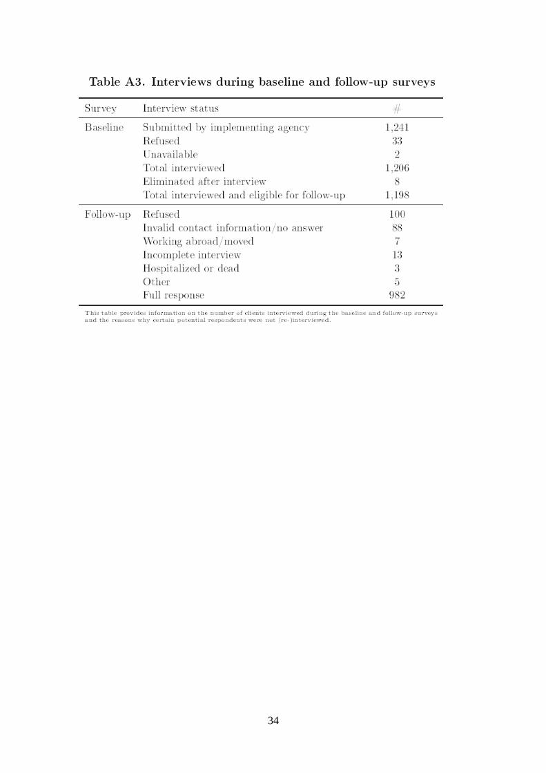
A total of 1,206 individuals were interviewed before the programme and 995 of these were
re-interviewed as part of the follow-up survey.18
The attrition rate was thus relatively low at
17 percent. Among other efforts to reinterview,19
people who initially declined were called
back later by a senior interviewer and asked once more to participate and were also offered a
€10 phone card.20
In the end, the response rate among the control group was about 10 per cent lower than in the
treatment group. Importantly, however, when we analyse the observed baseline
characteristics of only those who were surveyed at follow-up, we find that these
characteristics are still balanced between the treatment and control group (see column 4 in
Tables 1 and A4).21
Thus, this differential non-response is not correlated with any of the
observable characteristics we consider. To reinforce this, we regress the indicator variable of
whether the marginal client was re-interviewed at follow-up on the soft characteristics as
provided by the loan officers. The results are presented in Table A6 in the Appendix and
show that these characteristics are not jointly significant in determining attrition and this is
true independent of whether we account for other covariates. We conclude that it is unlikely
that attrition undermined the balanced nature of the treatment and control samples and
introduced bias in the reported results.
17 Table A5 in the Appendix contains the full regression results for this test. 18 Eight baseline respondents were not approved by the loan committee or decided not to borrow after all (thus
reducing the original baseline sample to 1,198). Thirteen of the 995 interviews were not fully completed. Table
A3 in the Appendix provides more details on the targeted and actual number of interviews at baseline and
follow-up. 19 In order to limit attrition, interviewers were trained to encourage participation and the survey company sent
all participants a reminder letter at the beginning of the follow-up survey. This letter also announced a raffle in
which all who completed the survey could take part. 20 The average yearly income of potential marginal clients was KM 13,381 at baseline. €10 (KM 19) therefore
corresponds to 54 per cent of average daily earnings. 21 We also checked that pre-treatment characteristics are balanced across treatment and control groups in the
following sub-samples: business ownership at baseline or not, high versus low education level, and gender of
the respondent. Lastly, we ran a regression in which the attrition dummy was regressed on treatment status, a set
of baseline characteristics, as well as the interaction terms between treatment status and the baseline covariates.
These interaction terms are jointly not statistically significant from zero.
9
4. Some theoretical considerations for interpreting the
results
In Appendix A2 we describe a simple model that can explain some of the key findings of our
paper. The main premise of the model is that investments are lumpy, in the sense that to start
up a business some minimum amount of capital is needed. In addition we assume that it is
more expensive to hire external labour because of taxes and regulatory costs. Under these
assumptions we show that for households that can make marginal investments, say because
they are already in business, an increase in the available loan amount will lead to increases in
both investments and consumption (for liquidity-constrained households). However, for
households that are facing minimum investment amounts (or indeed other start-up costs)
consumption and accumulated savings may decline if the loan amount is insufficient to cover
the start-up capital. In this case the household will crowd-in resources by running down other
assets and reducing consumption.
In addition some of these households may also reduce the schooling of their young adults
(16-19), that is, those facing the choice between schooling and work.22
This will only happen
for those whose expected returns to education are relatively low. In this case, and because of
the additional wedge caused by the regulation costs of hiring outside labour, young adults
who would have attended school in the absence of a home business will start working and
reduce schooling. Moreover the amount of schooling will decline more as the loan amount is
increased. In other words, we may see reductions in schooling for both start-up businesses
and existing ones. While the negative effect of the loans on consumption should only be
temporary, the reduction in schooling will persist even for established businesses when the
expected returns to education are relatively low and regulatory costs high. The reduction in
schooling does not necessarily point to an inefficiency or to an undesirable effect of
microcredit; if the returns to schooling are indeed very low, starting to work at home may be
the right thing to do. However, such reductions may also be due to parents not internalising
the entire benefits of schooling for their children or because of labour market distortions that
create a wedge between household and market labour.
Overall, the model generates four main predictions for households that receive access to
loans:
1. Consumption increases for households with an existing business as their liquidity
constraint is relaxed (with the proviso that marginal investments are not lumpy).
2. Consumption may decrease for those who start up a business if the loan is not large enough
to cover the initial costs.
3. Savings may decrease for those who are starting up a business.
4. Labour supply by young adults may increase and educational participation may decline, in
particular for those with lower expected returns to education.
The model predictions are not sharp because they depend on a number of factors we do not
observe, such as the extent to which profitable investments are lumpy and larger than the
22 Education in Bosnia and Herzegovina is free and compulsory for all children aged 7 to 15, while secondary
education remains free but is voluntary.

10
loan, and the expected returns to education. However they point to important features in the
results that we should be looking out for and they provide an interpretative framework.
4.1 Do borrowers make lumpy investments?
To examine the extent to which investments are lumpy we analyse reported loan use. A
limitation of this approach is that, although the information we collected on loan use is
detailed when compared with many other household surveys, the categories are still quite
broad. To give an example, we know whether a client used the loan for the purchase of
livestock but we do not know whether she bought, say, 20 chickens or one cow. Given such
limitations, this section only aims at providing some indicative evidence of the lumpiness of
the marginal borrowers' investments.
A first indication of lumpy investments is that on average borrowers used the loan for only
1.32 different purposes (with a standard deviation of 0.59). Thirty per cent of the loans have
been used exclusively for one single purpose. From Table 2 we can see that most loans are
used for purchasing livestock – 139 marginal clients (24 per cent of all clients) report this use
(columns 1 and 2). The average amount used for this purpose was KM 1,636 (~US$ 1,000)
(column 3) or about 77 per cent of the average loan amount (column 5). The remainder of
these loans were almost completely put towards buying auxiliary agricultural inputs such as
seed, fertiliser, and fodder (column 6).
The first two rows of Table 2 show that investments in livestock combined with buying seed,
fodder and other agricultural items is indeed very common. A large number of clients have
used practically the whole loan amount to start-up or to substantially expand an agricultural
activity. This suggests that borrowers had to cover some upfront costs that are more than
proportional to returns (that is, are lumpy) to make their investment.
11
5. Results
5.1 Main outcomes of interest and estimation strategy
We start by estimating the impact of microcredit on business ownership and start-up, business
profits and household income. We then consider consumption, savings and labour supply, the
latter particularly of young adults. We estimate separate treatment effects by splitting the
sample according to whether the household had a business at baseline or not and according to
the level of education of the marginal borrower. For the latter, we define “low education” as
having obtained no more than primary education and “high education” as any grade
completed above primary education.
We estimate the effects of the programme through a simple comparison of means of the
various outcomes of interest Y. To improve precision we include baseline covariates and
estimate the following equation using OLS:
(1)
where T is the treatment indicator (T=1 if the individual received a loan and T=0 if not) so
that α1 is the average treatment effect of being offered a loan for our population of loan
applicants. Xb is a set of baseline covariates that includes the respondent's age, gender, and
marital, educational and economic status. It also includes characteristics such as household
composition and the economic status and income level of the individual household members.
u is the error term. To estimate how the effect may vary with observable characteristics, we
repeat the estimation on suitably defined sub-samples.
5.2 Impact on business creation and development
We first look at the effect on enterprise creation and growth. Note that EKI did not monitor
the use of the loans and there were no sanctions of any sort if the loans were used for
purposes such as consumption.
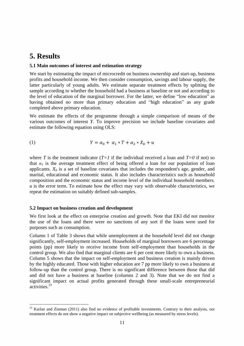
Column 1 of Table 3 shows that while unemployment at the household level did not change
significantly, self-employment increased. Households of marginal borrowers are 6 percentage
points (pp) more likely to receive income from self-employment than households in the
control group. We also find that marginal clients are 6 per cent more likely to own a business.
Column 5 shows that the impact on self-employment and business creation is mainly driven
by the highly educated. Those with higher education are 7 pp more likely to own a business at
follow-up than the control group. There is no significant difference between those that did
and did not have a business at baseline (columns 2 and 3). Note that we do not find a
significant impact on actual profits generated through these small-scale entrepreneurial
activities.23
23 Karlan and Zinman (2011) also find no evidence of profitable investments. Contrary to their analysis, our
treatment effects do not show a negative impact on subjective wellbeing (as measured by stress levels).
12
We also observe some interesting heterogeneity by education level in terms of the types of
businesses that are created. Those with no higher than primary education are more likely to
start up agricultural activities than the control group.
In contrast, those with a higher education are more likely to start up an enterprise in the
services sector. Table 4 shows that already at the time of the baseline survey there were some
sectoral differences according to education level (although these differences were not
statistically significant). Lastly, we note that the likelihood of owning inventory is
significantly higher (about 5 pp) for treatment than for control households. This effect is the
largest for marginal clients with at most primary education, who are 7 pp more likely to own
inventory at the end of the experiment.
Table 5 shows that while the percentage of business owners in our sample was about 62 per
cent at baseline (63 per cent in the treatment and 62 per cent in the control group) this had
decreased to 54 per cent at the time of the follow-up survey, most likely reflecting the severe
impact of the financial crisis on small-scale entrepreneurs. Thus the programme impact was
to reduce the decline in business ownership during the financial crisis, a possible reflection of
the importance of credit in propagating the crisis. The difference is driven both by fewer
existing businesses closing and more new ones opening among the treated respondents.
Overall, about 35 per cent of business owners in our sample closed their business between the
two survey rounds, and only 14 per cent started one over this period.

13
5.3 Impact on consumption and savings
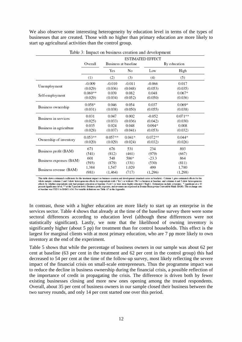
Table 6 shows the estimated impacts on a number of consumption measures. The first row
shows the effect on the household's overall consumption expenditure, which includes money
spent on food (inside and outside of the house), other non-durables (such as rent, bills, clothes
and recreation) and durables (large, infrequent purchases which here include educational
expenses, the purchase of vehicles and vacations).24
24 Food expenditures were collected over a recall period of a week, other non-durables over a period of a month,
and durables over a period of a year. To calculate the aggregate spending amount we assume that the week and
month about which the household was asked were representative for the year. This assumption is not important
in view of the impact analysis (as we compare treatment and control groups over the same period) but does play
a role when we put the value of expenditures in context, for instance by comparing them to income.
14
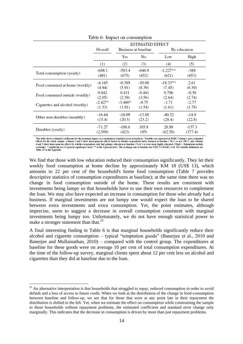
We find that those with low education reduced their consumption significantly. They let their
weekly food consumption at home decline by approximately KM 18 (US$ 13), which
amounts to 22 per cent of the household's home food consumption (Table 7 provides
descriptive statistics of consumption expenditures at baseline); at the same time there was no
change in food consumption outside of the home. These results are consistent with
investments being lumpy so that households have to use their own resources to complement
the loan. We may also have expected an increase in consumption for those who already had a
business. If marginal investments are not lumpy one would expect the loan to be shared
between extra investments and extra consumption. Yet, the point estimates, although
imprecise, seem to suggest a decrease in overall consumption consistent with marginal
investments being lumpy too. Unfortunately, we do not have enough statistical power to
make a stronger statement than that.25
A final interesting finding in Table 6 is that marginal households significantly reduce their
alcohol and cigarette consumption – typical “temptation goods” (Banerjee et al., 2010 and
Banerjee and Mullainathan, 2010) – compared with the control group. The expenditures at
baseline for these goods were on average 10 per cent of total consumption expenditures. At
the time of the follow-up survey, marginal clients spent about 12 per cent less on alcohol and
cigarettes than they did at baseline due to the loan.
25 An alternative interpretation is that households that struggled to repay, reduced consumption in order to avoid
default and a loss of access to future credit. When we look at the distribution of the change in food consumption
between baseline and follow-up, we see that for those that were at any point late in their repayment the
distribution is shifted to the left. Yet, when we estimate the effect on consumption while constraining the sample
to those households without repayment problems, the estimated coefficient and standard error change only
marginally. This indicates that the decrease in consumption is driven by more than just repayment problems.
15
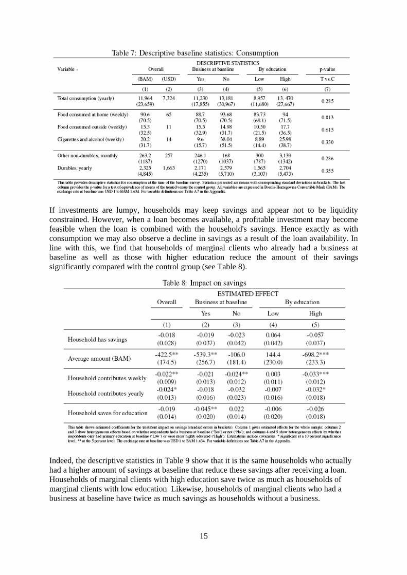
If investments are lumpy, households may keep savings and appear not to be liquidity
constrained. However, when a loan becomes available, a profitable investment may become
feasible when the loan is combined with the household's savings. Hence exactly as with
consumption we may also observe a decline in savings as a result of the loan availability. In
line with this, we find that households of marginal clients who already had a business at
baseline as well as those with higher education reduce the amount of their savings
significantly compared with the control group (see Table 8).
Indeed, the descriptive statistics in Table 9 show that it is the same households who actually
had a higher amount of savings at baseline that reduce these savings after receiving a loan.
Households of marginal clients with high education save twice as much as households of
marginal clients with low education. Likewise, households of marginal clients who had a
business at baseline have twice as much savings as households without a business.

16
Combining these results with the findings on consumption and our model predictions, it
seems that the loan offered during the experiment relaxed liquidity constraints but only up to
a certain extent. Households still had to find additional resources to be able to invest the
minimum amount of capital that was needed. Those households that already had a business
and those that have higher education (a typical proxy for higher income) could do so by
running down their savings. In contrast, low-educated households did not have enough
savings and hence reduced their consumption.
5.4 Impact on hours worked and school attendance
An implication of our interpretative framework is that young adults (16-19) may start to work
more when capital constraints are relaxed, particularly those with a lower expected return to
schooling. We do not have information on the perceived return to schooling, but use the
educational status of their parents as a proxy, based on the idea that poorer and less-educated
parents invest less in their children, which may lead to lower returns to education.
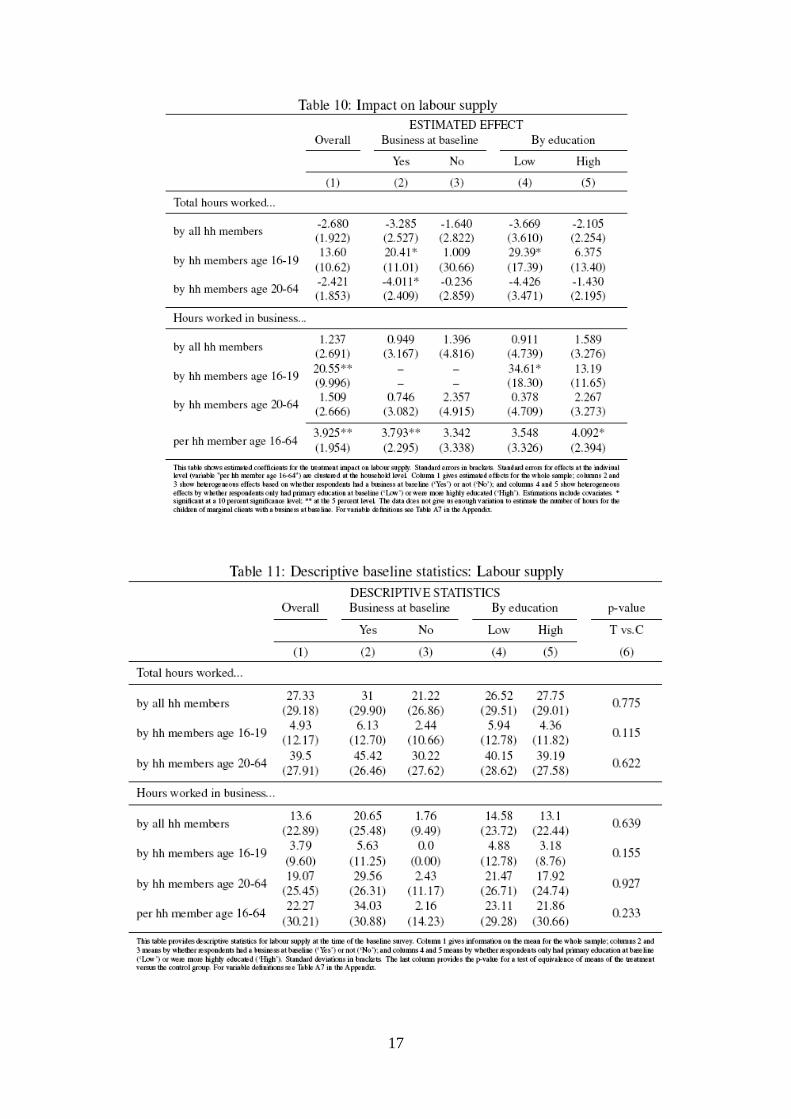
Table 10 displays the impact on labour supply. The upper panel looks at total hours worked
and the lower panel at hours in the household business. While we do not find a change in the
overall hours worked by the household as a whole, we do find strong impacts for children and
young adults aged 16-19. These young household members work significantly more,
compared with the control group, if their household already had a business at baseline or if
the borrower had no higher than primary education. In particular, children of marginal clients
with a business at baseline work on average 20 hours per week more than children of the
same age in the control group. And children of marginal clients with no higher than primary
education work on average 29 hours more than the control group.26
26 Table 11 provides descriptive statistics for the number of hours worked at the time of the baseline survey by
household members of various age groups.
17

18
The lower panel of Table 10 shows that the additional hours worked are indeed spent in the
business. Children aged 16-19 of low-educated households work on average 35 hours per
week more in the business compared with the control group. The bottom row shows that the
hours of work per household member increased by about 4 as a result of microcredit, showing
an increased overall effort and not just substitution between members of the household.
We now examine whether the increase in working hours is indeed accompanied by a decrease
in school attendance for young adults. Table 12 indicates that this is indeed the case. We
estimate the effect of the intervention on the likelihood of attending school for each
household member younger than 20 years and compare different age groups. School
attendance decreases significantly for teenage children aged 16-19. The results suggest that
they are 9 per cent less likely to attend school due to the intervention. This overall effect is
driven by the children of marginal clients with at most primary education – those for whom
we also observe an increase in working hours. Due to the microcredit programme, teenage
children aged 16-19 in these households are in fact 19 per cent less likely to attend school
than in the control group. Table 13 shows that children of households with lower education
levels were already less likely to attend secondary school before the programme started
(again, this was not significantly different between treatment and control households). The
intervention seems to have reduced schooling further, consistent with the idea that
households with lower perceived returns to education (as may be those with low education)
find the opportunity of having their children work in the household business more attractive
than education.

19
5.5 Does gender matter?
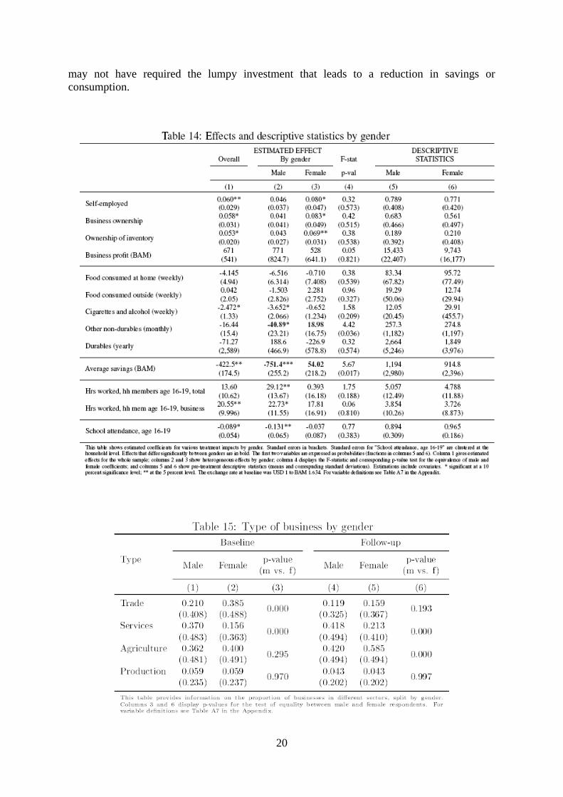
About 40 per cent of the marginal clients are female. Table 14 displays estimated impacts, for
a subset of our outcome variables, for both the sample as a whole as well as by gender. We
uncover an interesting pattern. The effect on business creation and the likelihood of being
self-employed seems to be mainly driven by female clients, who as a result of access to credit
are 8 per cent more likely to be self-employed and to own a business compared with the
control group. These women also are 7 per cent more likely to own business inventory.
In contrast, the other effects reported above appear to be mainly driven by male borrowers. It
is male marginal clients who decrease household savings and cut back consumption
(cigarettes and alcohol as well as other non-durable consumption). And it is these variables
(“other non-durables” and “average savings”) where the gender difference in impact is
statistically significant at the 5 per cent level. Moreover, it is also male marginal clients in
whose households young adults work significantly more (in general as well as in the
business) and are significantly less likely to attend school. In fact, teenagers who just
completed mandatory schooling and live in households of male marginal clients are 13 per
cent less likely to attend school than teenagers of the same age group in control households.
A possible explanation is that access to credit allowed men to expand and scale-up pre-
existing businesses, whereas women created new businesses. If these new female-operated
businesses were very small there was no need to supplement the loan with existing savings, to
reduce consumption or to take young adults out of school. In contrast, male borrowers that
expanded existing businesses may have only been able to do so by crowding in resources
from savings, reducing consumption and using the labour of teenage household members.
Table 15 provides some supportive evidence for this idea. It shows that between the baseline
and follow-up survey, there was a sharp reduction in the proportion of enterprises that
engaged in trade. This likely reflects the sudden and strong negative impact of the financial
crisis on trade flows. As a result, the services and agricultural sectors became relatively more
important for both men and women. However, women seem to have shifted to agricultural
activities in particular: at follow-up about 60 per cent of all female enterprises were
agricultural in nature. To the extent that such newly established “enterprises” were informal
and small-scale, mainly reflecting the difficult economic environment during the crisis, they
20
may not have required the lumpy investment that leads to a reduction in savings or
consumption.

21
6. Commercial viability of the programme
To put the borrower impacts into context, we proceed with a concise analysis of the
profitability, and therefore commercial viability, of lending to marginal borrowers. We
analyse both the profitability in absolute terms and relative to EKI's regular lending
operations over the same period.
To assess the profitability of the marginal lending programme we compare two groups of
loans. First, we analyse all loans disbursed to marginal clients between December 2008 and
May 2009, the period of the experiment, and that were due by June 2012 at the latest. Second,
we analyse all loans disbursed to regular first-time clients during the same period. We focus
on first-time regular clients for comparability reasons as all marginal clients are by definition
first-time borrowers of our MFI. For both groups we take into account all regular and late
payments that were made. Table 16 provides general statistics on these two groups of clients.
For ease of comparison, we also present the same statistics for all regular EKI clients,
whether they are first-time or repeat clients.
It becomes clear that the new marginal client group was significantly more risky than either
first-time or all regular EKI clients. In particular, late payment (column 4) is 1.5 times as high
among marginal clients compared with regular first-time clients (46 versus 31 percent) while
in the end non-repayment (column 5) among the marginal clients is even three times as high
compared with regular clients (26 versus 9 percent). We find no significant differences in
repayment between men and women in either borrower group.
To better understand how these significant differences in non-repayment affected the
commercial viability of the programmes, we calculate the net present value (NPV) of both the
marginal and the regular lending programmes. For each programme, we first sum up all the
discounted outgoing (loan disbursements) and incoming (repayments, fee income and interest
revenue) cash flows. As a discount rate we use EKI's weighted-average cost of debt funding
in March 2011 (where we weigh by the size of individual outstanding liabilities). Since EKI
uses both commercial and concessional funding, we use three discount rates: one based on

22
the (weighted cost of) its commercial funding, one based on the (weighted cost of) its
concessional funding; and one based on the (weighted cost of) all funding.27
We then divide
these NPVs by the total amount of loans granted under the programme to calculate an overall
rate of return. In addition, we also calculate an internal rate of return (IRR) of both lending
programmes (the discount rate at which the net present value of the sum of all cash flows
equals zero). Table 17 summarises these calculations.
We find that the rate of return on the marginal-lending programme is negative – regardless of
the discount rate that we apply – and that the IRR is minus 11 percent. Although EKI charges
an interest rate of 22 per cent per year, the lending programme was not profitable due to a
high level of non- and late repayments. As mentioned, 26 per cent of the loans had to be
written off and 46 per cent of the borrowers were at least once late with monthly repayments.
Although the rate of return on loans to female marginal clients was slightly lower than on
loans to male clients, this difference is not statistically significant.
While the lending programme to marginal clients was not profitable during our sample
period, one should keep in mind that Bosnia and Herzegovina went through a deep economic
crisis at the time of the experiment. It is therefore important to compare the profitability of
our experimental borrowers with the benchmark of regular EKI clients.
27 EKI receives concessional funding from various NGOs and development institutions. The average
concessional funding rate is just under 40 per cent of the costs of its commercial funding.

23
Table 17 shows that during the same period the internal rate of return of EKI's regular
lending business was positive, at 14 per cent for first-time borrowers. Of the regular loans to
first-time borrowers 9 per cent had to be written off and 31 per cent of the clients were at
least once late with repaying (Table 16). This implies that the “marginal clients” were
substantially worse risks compared with regular clients and in the end loss-making.
Overall, we conclude that the programme was not commercially viable, at least in this period
of financial crisis. If we add up the total amount of loans that were never paid back by the
marginal borrowers, as well as the foregone interest on these loans, and then divide this
amount by the total number of marginal borrowers, we arrive at an implicit subsidy by EKI to
the average marginal borrower of KM 387 (US$ 268). This corresponds to approximately one
fourth of the average loan amount extended to marginal borrowers.
To get a better understanding of why marginal borrowers are more risky, we ran a set of
probit regressions on a sample that contains both the regular and the marginal clients. The
dependent variable is a default indicator. Table 18 summarises our results. The probability of
default is 17 percentage points higher for marginal than for regular clients (this corresponds
to the difference between the 26 and 9 per cent write-offs in Table 16). In column 2, we add a
set of borrower characteristics that are both observable to the loan officer and the
econometrician (such as the borrower's age, gender, and marital, educational and economic
status). The marginal client dummy stays statistically significant at the 1 per cent level and
the coefficient is only marginally reduced in size. This shows that even when controlling for
basic borrower characteristics, marginal clients were inherently more risky. It appears that
loan officers, using “soft” information (Berger and Udell, 1995) about less readily observable
borrower characteristics, have been able to adequately distinguish between marginal and
regular clients. The marginal client dummy also remains statistically significant and the
coefficient size does not change much when we add branch fixed effects (column 3). This
implies that there was no substantial cross-branch variation in average default levels, for
example due to geographic heterogeneity in borrower risk or an uneven quality of loan
officers between branches.

24
We further explore the idea that loan officers use soft information effectively when making
decisions about loan applicants by using our data on loan officers' perceptions of marginal
clients, previously discussed in Section 2.2. Table 19 shows the results of regressions where
the dependent variable is either an indicator of whether a marginal client was at least once
late with repaying a loan instalment (columns 1-4) or a default indicator (columns 5-8). In
columns 1-2 and 5-6 we only include three regressors that indicate whether a loan officer
thought that an applicant satisfied EKI's standard requirements in terms of collateral,
repayment capacity and credit history. In columns 3-4 and 7-8 we add loan officers'
judgments of various character traits of the marginal clients. Columns 2, 4, 6 and 8 contain
the covariates and branch fixed effects that we used in Table 18.
We find a positive correlation between compliance with EKI's collateral requirement and late
payment though not with actual default. This correlation becomes imprecisely estimated once
we add the various other soft and hard client characteristics. The fact that we find a positive
correlation between collateral and late payments is an interesting indication of adverse
selection: to be a marginal client despite having collateral reveals other strong negative
(unobserved) characteristics relating to repayment capacity.
In terms of the relationship between (ex ante measured) personality traits and repayment
behaviour, we find that the estimated coefficients for these traits have the expected sign.
Borrowers that were judged to be relatively competent and stable turn out to be less likely to
pay late or to default, whereas the opposite holds for those that were deemed to be aggressive
and risk-takers.
25
Even when we include a set of easily observable borrower covariates as well as branch fixed
effects, we find that some of these characteristics remain significantly correlated with
repayment behaviour. This suggests that EKI's loan officers not only effectively used
information on applicants' characteristics to distinguish between regular and marginal clients
but also to differentiate among marginal clients. This raises the question whether simple
credit scoring is perhaps less effective than the face-to-face assessment by loan officers;
however one also needs to compare the costs of each approach.
7. Conclusion
This paper presents results from a field experiment in Bosnia and Herzegovina in which a
random selection of potential borrowers received one or more loans from a local
microfinance institution. We find that access to borrowing (partially) relaxed the liquidity
constraints of the treatment group and had a positive impact on business creation and
survival. One year after the start of the programme, marginal borrowers were 6 per cent more
likely to own an enterprise compared with the control group. Borrowers with higher
education levels mainly started businesses in the services sector whereas the less educated
established small-scale agricultural activities. Those households that already had a business
and those that were highly educated ran down their savings. In contrast, less-educated
households reduced consumption. This is consistent with investments being lumpy so that
households need to crowd in additional resources to make up the difference and to implement
investments that would have been unattainable without the loan.
We also document that households of marginal clients with low education levels reduced the
school attendance of their teenagers (aged 16-19) and let them work more in the household's
business instead. On average these children work 35 hours per week more in this business
compared with the control group and, not surprisingly, are 19 per cent less likely to attend
school. Teenage children of marginal clients who had a business at baseline also work more
in the business, but their school attendance is not reduced significantly when compared with
the control group. As yet, there is not much evidence that the small-scale and often
agricultural activities of lower-educated families will generate positive revenues that more
than offset the loss in future income due to children's lower human capital.
The findings paint a mixed picture of the impact of microcredit. On the one hand, households
did use the loans to start up new businesses, to keep existing ones afloat, or to expand them.
Where necessary they even cut back on consumption and used their savings to make
sufficiently large investments. On the other hand, we do not find that these entrepreneurial
activities had a positive impact on income. Even for households that already had an enterprise
at the time of the baseline survey, and for whom our model predicts an increase in
consumption, we do not find such a positive impact.28
Moreover, we document that the
program was not profitable: EKI in fact provided an implicit subsidy to the average marginal
borrower of US$ 268.
There are various possible reasons why we do not (yet) find evidence of a positive impact of
microcredit on enterprise profits, household income, or consumption, notwithstanding an
increase in entrepreneurial activity. First, the period between our baseline and follow-up
surveys – about 14 months – may have been too short to allow households to fully implement
investments and increase firm profitability. Households that cut back consumption when they
received a loan will have done so in the expectation that their investment will lead to higher
28 Crépon et al. (2011) also find that households with a pre-existing enterprise decrease consumption as they
save and borrow to scale up their activities.

26
future consumption. While profitability may thus still increase over time, one should also
keep in mind that the businesses were mainly in the services and agricultural sectors and
quite straightforward in nature. After loan disbursal, borrowers should in most cases have
been able to implement investments and reap their pay-offs quite quickly.
An alternative explanation is that access to finance may not be the only binding constraint on
entrepreneurial activity. Bruhn and Zia (2011) use an RCT to study the impact of a business
and financial literacy programme on the firms of young Bosnian entrepreneurs, all of whom
were borrowers from a local MFI. They find that while training did not influence business
start-up or survival, it significantly improved business practices, investments and loan terms
for surviving firms. An interesting area for future research is therefore to uncover what
combinations of credit and training can help stimulate entrepreneurship not only at the
intensive but also at the extensive margin.

27
References
D. Acemoglu and J.-S Pischke (1999), “The Structure of Wages and Investment in General
Training”, Journal of Political Economy 107, 539-572.
J.G. Altonji (2005), “Employer Learning, Statistical Discrimination, and Occupational
Attainment”, American Economic Review Papers and Proceedings 95, no. 2: 112-117.
O. Attanasio, B. Augsburg, R. De Haas, E. Fitzsimons and H. Harmgart (2011), “Group
Lending or Individual Lending? Evidence from a Randomized Field Experiment in
Mongolia”, EBRD Working Paper No. 136, European Bank for Reconstruction and
Development, London.
A. Banerjee, E. Duflo, R. Glennerster and C. Kinnan (2010), “The Miracle of Microfinance?
Evidence from a Randomized Evaluation”, BREAD Working Paper No. 278.
A. Banerjee and S. Mullainathan (2010), “The Shape of Temptation: Implications for the
Economic Lives of the Poor”, NBER Working Paper No. 15973.
K. Beegle, R.H. Dehejia and R. Gatti (2006), “Child Labour and Agricultural Shocks”,
Journal of Development Economics 81, no. 1: 80-96.
A.N. Berger and G.F. Udell (1995), “Relationship Lending and Lines of Credit in Small
Business Finance”, Journal of Business 68, 351-382.
M. Bruhn and B. Zia (2011), “Stimulating Managerial Capital in Emerging Markets: The
Impact of Business and Financial Literacy for Young Entrepreneurs”, World Bank
Policy Research Paper no. 5642, World Bank, Washington DC.
D. Collins, J. Morduch, S. Rutherford and O. Ruthven (2009), “Portfolios of the Poor: How
the World's Poor Live on $2 a Day”, Princeton University Press, Princeton, New
Jersey.
B. Crépon, F. Devoto, E. Duflo W. Parienté (2011), “Impact of Microcredit in Rural Areas of
Morocco: Evidence from a Randomized Evaluation”, MIT Working Paper.
S. De Mel, D. McKenzie and C. Woodruff (2009), “Are Women More Credit Constrained?
Experimental Evidence on Gender and Micro-Enterprise Returns”, American Economic
Journal: Applied Economics 1, no. 3: 1-32.
A. Demirgüc-Kunt, L.F. Klapper and G.A. Panos (2011), “Entrepreneurship in Post-Conflict
Transition – The Role of Informality and Access to Finance”, Economics of Transition,
19, no. 1: 27-78.
European Commission (2010), “Bosnia and Herzegovina 2010 Progress Report”, Brussels.
M. Fafchamps, D. McKenzie, S. Quinn and C. Woodruff (2011), “When is Capital Enough to
Get Female Microenterprises Growing? Evidence from a Randomized Experiment in
Ghana, World Bank Policy Research Working Paper no. 5706, World Bank,
Washington D.C.
E. Field and R. Pande (2008), “Repayment Frequency and Default in Micro-Finance:
Evidence from India”, Journal of the European Economic Association 6, no. 2-3: 501-
9.
B. Feigenberg, E. Field and R. Pande (2010), “Building Social Capital through
Microfinance”, NBER Working Paper no. 16018, National Bureau of Economic
Research, Cambridge, M.A.
28
M. Ghatak and T. Guinnane (1999), “The Economics of Lending with Joint Liability: A
Review of Theory and Practice”, Journal of Development Economics 60, 195-228.
X. Giné, P. Jakiela, D. Karlan and J. Morduch (2010), “Microfinance Games”, American
Economic Journal: Applied Economics 2, 60-95.
X. Giné and D. Karlan (2010), “Group Versus Individual Liability: Long-Term Evidence
from Philippine Microcredit Lending Groups”, mimeo.
V. Hartarska and D. Nadolnyak (2007), “An Impact Analysis of Microfinance in Bosnia and
Herzegovina”, William Davidson Institute Working Paper no. 915, University of
Michigan.
H.G. Jacoby (1994), “Borrowing Constraints and Progress through School: Evidence from
Peru”, Review of Economics and Statistics 76, no. 1: 151-160.
H.G. Jacoby and E. Skoufias (1997), “Risk, Financial Markets, and Human Capital in a
Developing Country”, Review of Economic Studies 64, 311-335.
J.P. Kaboski and R.M. Townsend (2005), “Policies and Impact: An Analysis of Village-Level
Microfinance Institutions”, Journal of the European Economic Association 3, no. 1: 1-
50.
D. Karlan and J. Zinman (2010), “Expanding Credit Access: Using Randomized Supply
Decisions to Estimate the Impacts”, Review of Financial Studies 23, no. 1: 433-464.
D. Karlan and J. Zinman (2011), “Microcredit in Theory and Practice: Using Randomized
Credit Scoring for Impact Evaluation”, Science 332, June: 1278-1284.
T. Kring (2004), “Microfinance as an Intervention against Child Labour in Footwear
Production in the Philippines”, Working Paper no.12, School of Development Studies,
University of Melbourne, Melbourne.
K. Maurer and J. Pytkowska (2011), “Indebtedness of Microfinance Clients in Bosnia and
Herzegovina. Results from a Comprehensive Field Study”, European Fund for
Southeast Europe (EFSE) Development Facility, mimeo.
N. Menon (2005), “The Effect of Investment Credit on Children’s Schooling: Evidence from
Pakistan”, mimeo, Brandeis University.
J. Morduch (1998), “Does Microfinance Really Help the Poor? New Evidence on Flagship
Programs in Bangladesh”, Princeton University Working Paper.
J. Morduch and D. Roodman (2009), “The Impact of Microcredit on the Poor in Bangladesh:
Revisiting the Evidence”, Center for Global Development Working Paper no. 174
(revised in December 2011).
L. Nelson (2011), “From Loans to Labor: Access to Credit, Entrepreneurship and Child
Labor”, mimeo, University of California, San Diego.
M. Pitt and S. Khandker (1998), “The Impact of Group-based Credit Programs on Poor
Households in Bangladesh: Does the Gender of Participants Matter?”, Journal of
Political Economy 106, no. 5: 958-98.
D. Roodman (2012), “Due Diligence. An Impertinent Inquiry into Microfinance”, Center for
Global Development, Washington, D.C.
B. Wydick (1999), “The Effect of Microenterprise Lending on Child Schooling in
Guatemala”, Economic Development and Cultural Change 47, no. 4: 853–869.

29
Appendix
A1 Characteristics of marginal clients
When identifying marginal clients, loan officers followed EKI's regular screening procedures
as closely as possible. Since the decision on whether a loan applicant was marginal or not
was not based on a credit-scoring system but on the loan officers' judgment, we asked loan
officers to fill in a questionnaire about each marginal client. This questionnaire elicited a
number of both objective and subjective assessments in order to help us better understand the
composition of our population. Of course we cannot compare these with the traits of the
regular clients. Our only benchmark in this exercise is whether the clients satisfy the
requirements for regular clients.
First, loan officers had to indicate whether they thought that the client conformed with EKI
requirements regarding the amount of available collateral, repayment capacity (based on
estimated cash flows), the client's overall creditworthiness, his or her business capacity and
lastly the client's credit history (if any). We find that the average marginal applicant did not
meet 2.6 out of six main EKI requirements. Table A1 shows that most marginal credit
applicants were considered marginal because they did not possess sufficient collateral (77
percent) or did not meet one or more of the “other” requirements, which include an
assessment of the applicant's character. About one in three marginal clients were judged to
have a weak business proposal while loan officers worried about repayment capacity in about
a quarter of the marginal applications. Loan officers were also asked which aspects of a
potential marginal client they thought were most and least worrisome. The last two columns
of Table A1 show that (a lack of) collateral was seen as most worrisome. On the other hand,
loan officers report to be least concerned about credit history, which is less relevant for first-
time borrowers, or the client's repayment and business capacity.
Second, because the loan officer's view of the applicant's character also feeds into the
decision to provide a loan or not, we asked loan officers to rate a number of personality traits
on a scale of 1 to 5 (1 representing total agreement and 5 total disagreement). These traits
included whether they perceived the marginal client to be competent, reliable, aggressive,

30
trustworthy and so on. Table A2 (columns one and two) shows descriptive statistics for a
summary indicator where agreement (“totally agree” and “agree”) is coded as one and
disagreement (“somewhat agree”, “disagree”, and “totally disagree”) as zero. The biggest
“gaps” are perceived to be in the applicants' knowledge (almost 50 per cent are not perceived
as knowledgeable) and their integration into society (more than 50 per cent are not seen as
well integrated). We also asked loan officers whether each of these character traits would
influence the prospective client's business success. From the third column in Table A2 we can
see that if a marginal client was perceived to be insecure, loan officers typically believed this
insecurity would have an impact on the client's business. Likewise, if a client was
characterised as a risk-taker, then loan officers thought in about 70 per cent of the cases that
this trait would influence the success of the business.

31
A2 Relaxing liquidity constraints when investments are lumpy: a simple model
To structure a unified interpretation of our empirical findings, this Appendix develops a
simple model of investment decisions when production requires a minimum amount of
capital in order to make lumpy investments. The model describes two periods. In the first
period the household can invest in a business that will produce output to be consumed in the
second period. A minimum level of capital Γ is required to produce, so that the production
function is Q=1(K> Γ)δKαH
1-α, where Q is output, K is capital and H is total labour
employed. The rate of time preference is equal to the interest rate r and the discount factor is
β=1/(1+r). The household includes a young adult who can either go to school in the first
period, and earn a lifetime return of s, or work. We model the return to education as
increasing the efficiency units of labour. An untrained person has one unit of labour. With
school attendance maximum efficiency units become ̂ ( ) where is the
schooling attendance in period one. Since leisure does not yield utility here, the individual
will work ̂ in the second period. Let the wage rate per efficiency unit be w. Preferences are
described by
(A1) ( )
We assume the household is liquidity constrained. However, we take the case where the
returns to education are high enough to imply zero labour supply in the absence of a home
business. At lower returns to education there will be an interior solution to young adult labour
supply even in the absence of a household business. Household income in the first period is
Y1 and in the second period Y2> Y1. We assume that the household can borrow up to an
amount ̅ (the microloan) and invests an amount K. It only uses internal labour (for
simplicity): external labour is assumed more expensive because of taxes and regulatory costs
that can be evaded/avoided when hiring internal labour. We also only consider the case where
the loan is not large enough to alleviate liquidity constraints. Hence the household maximises
lifetime utility subject to the two constraints
(A2) ̅
and
(A3) ( ( )) ( )
where R is the gross return payable for the loan and foregone future returns to education is
the opportunity cost of labour. Given the optimal level of investment K>Γ the solution to the
problem is

32
( ( ))
( )
(A4)
where [
( ) ]
and [ ]
. In the absence of investment and the loan
c1=Y1 (assuming a corner solution for labour, that is, full-time education and liquidity
constraints). Now a marginal increase in the loan will increase both consumption and
investment. However a switch from zero investment to a positive amount (over Γ) can lead to
a decline in consumption as K can be larger than B for high enough return (a high enough δ
will deliver this). Young adult labour also increases with investment. More importantly, for
those with low enough returns to education (but high enough to go to school in the absence of
a home business) l1 will switch to a positive amount from zero as the household starts a
business. If returns to education are high enough then the opportunity cost of internal labour
increases and the household may hire the more expensive external labour instead. In this
sense we expect young adult labour to go up for households where the returns to education
are (perceived to be) low, which is likely to include many of the poorer households. The jump
will be larger for those with no business at baseline.

33
Chart A1a Geographical location of participating branches
Chart A1b Geographical location of treatment and control households
34

35

36

37

38
39
40


