Logistic Regression
Sociology 229: Advanced Regression
Copyright © 2010 by Evan SchoferDo not copy or distribute without permission

Announcements
• None

Agenda
• Today’s Class• Introductions • Go over syllabus• Review topic: Logistic regression
– Not required – only for those who want to stay…
• Next week:• Multinomial logistic regression
Introduction
• Goal of this course: expand your methodological “toolbox”– Regression is extremely robust and versatile...
• BUT: often we have data that violates assumptions of regression models…
– Such as a dichotomous dependent variable
• OR: we wish to do a kind of analysis beyond what can be done with ordinary regression models
– Ex: quantile regression
– So, we need to develop a set of additional tools…

Introduction
• Main course topics• Multinomial logistic regression• Count models• Event history / survival analysis• Multilevel models & panel models
– & some additional stuff squeezed in…
• Issue: There is always a trade-off between depth and coverage
• The course covers a lot of topics briefly• Advantage: exposes you to lots of useful things• Disadvantage: We don’t have nearly enough time to
cover material thoroughly…

Review Syllabus
• Main points:• All readings are available online
– Complete readings prior to class on week they are assigned
• Grades are based on several short assignments – Plus, small “participation” component– No big paper at the end
– NOTE: This class has some overlap with my Event History Analysis class
• I’ve come up with some (optional) alternative material for those who took my earlier class.

Introductions
• This is a small class… let’s introduce ourselves
• Also: It is helpful to get to know your classmates… for when you are stuck on the homework…
Review: Types of Variables
• Continuous variable = can be measured with infinite precision
• Age: we may round off, but great precision is possible
• Discrete variable = can only take on a specific set of values
• Typically: Positive integers or a small set of categories• Ex: # children living in a household; Race; gender• Note: Dichotomous = discrete with 2 categories.

Review: Types of Variables
• And, don’t forget about measurement scales:
• Nominal: Categories that can’t be ordered• Note: Also called “categorical” variables • Ex: Religion; race; geographic state of residence
• Ordinal: Orderable categories• Ex: Social class; College “rankings”; Most attitudinal
measures (Do you approve of… on a 1-5 scale)
• Interval/Continuous: Ordered, with consistent differences across units
• Ex: Age; Cholesterol level; Income (in dollars).
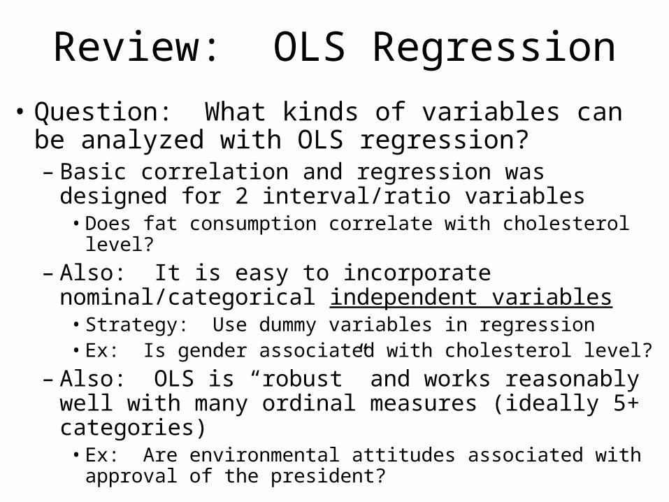
Review: OLS Regression
• Question: What kinds of variables can be analyzed with OLS regression?– Basic correlation and regression was designed for
2 interval/ratio variables• Does fat consumption correlate with cholesterol level?
– Also: It is easy to incorporate nominal/categorical independent variables
• Strategy: Use dummy variables in regression• Ex: Is gender associated with cholesterol level?
– Also: OLS is “robust” and works reasonably well with many ordinal measures (ideally 5+ categories)
• Ex: Are environmental attitudes associated with approval of the president?

Example 1: OLS Regression• Example: Study time and student achievement.
– X variable: Average # hours spent studying per day– Y variable: Score on reading test
Case X Y
1 2.6 28
2 1.4 13
3 .65 19
4 4.1 31
5 .25 8
6 1.9 16
Y axis
X axis
0 1 2 3 4
30
20
10
0
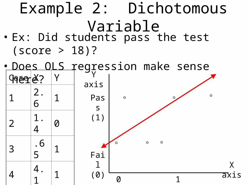
Example 2: Dichotomous Variable• Ex: Did students pass the test (score > 18)?
• Does OLS regression make sense here?
Case X Y
1 2.6 1
2 1.4 0
3 .65 1
4 4.1 1
5 .25 0
6 1.9 0
Y axis
X axis
0 1 2 3 4
Pass (1)
Fail (0)

OLS & Dichotomous Variables
• Problem: OLS regression wasn’t really designed for dichotomous dependent variables
• Two possible outcomes (typically labeled 0 & 1)
• What kinds of problems come up?– Linearity assumption doesn’t hold up– Error distribution is not normal– The model offers nonsensical predicted values
• Instead of predicting pass (1) or fail (0), the regression line might predict -.5.
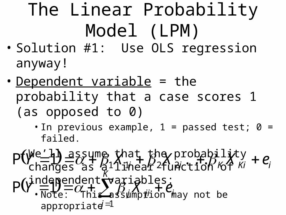
The Linear Probability Model (LPM)
• Solution #1: Use OLS regression anyway!
• Dependent variable = the probability that a case scores 1 (as opposed to 0)
• In previous example, 1 = passed test; 0 = failed.
– We’ll assume that the probability changes as a linear function of independent variables:
• Note: This assumption may not be appropriate
iKiKii eXXXY ...1P 2211
i
K
jjij eXY
1
1P
Linear Probability Model (LPM)
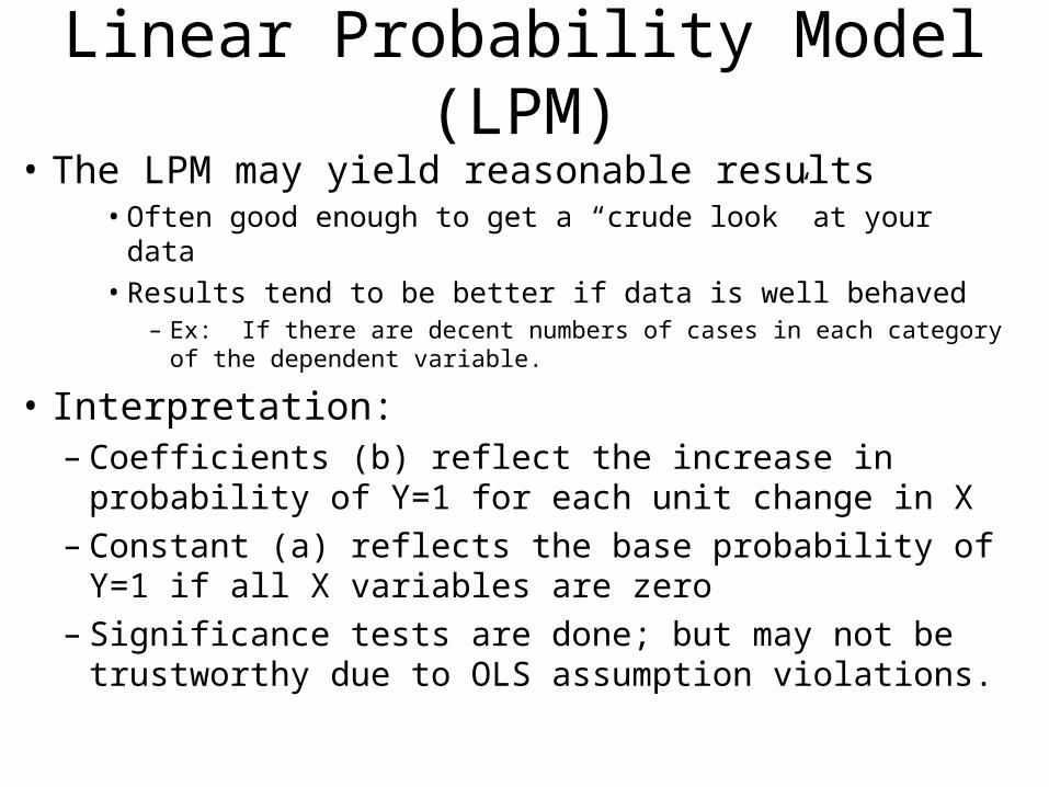
• The LPM may yield reasonable results• Often good enough to get a “crude look” at your data• Results tend to be better if data is well behaved
– Ex: If there are decent numbers of cases in each category of the dependent variable.
• Interpretation:– Coefficients (b) reflect the increase in probability
of Y=1 for each unit change in X– Constant (a) reflects the base probability of Y=1 if
all X variables are zero– Significance tests are done; but may not be
trustworthy due to OLS assumption violations.
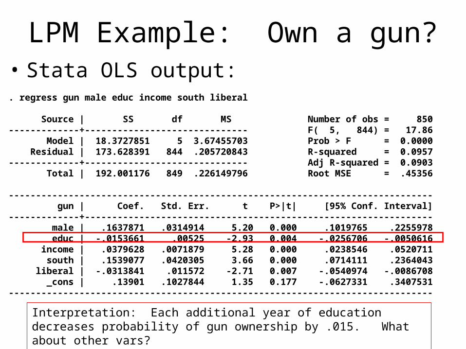
LPM Example: Own a gun?• Stata OLS output:. regress gun male educ income south liberal
Source | SS df MS Number of obs = 850-------------+------------------------------ F( 5, 844) = 17.86 Model | 18.3727851 5 3.67455703 Prob > F = 0.0000 Residual | 173.628391 844 .205720843 R-squared = 0.0957-------------+------------------------------ Adj R-squared = 0.0903 Total | 192.001176 849 .226149796 Root MSE = .45356
------------------------------------------------------------------------------ gun | Coef. Std. Err. t P>|t| [95% Conf. Interval]-------------+---------------------------------------------------------------- male | .1637871 .0314914 5.20 0.000 .1019765 .2255978 educ | -.0153661 .00525 -2.93 0.004 -.0256706 -.0050616 income | .0379628 .0071879 5.28 0.000 .0238546 .0520711 south | .1539077 .0420305 3.66 0.000 .0714111 .2364043 liberal | -.0313841 .011572 -2.71 0.007 -.0540974 -.0086708 _cons | .13901 .1027844 1.35 0.177 -.0627331 .3407531------------------------------------------------------------------------------
Interpretation: Each additional year of education decreases probability of gun ownership by .015. What about other vars?
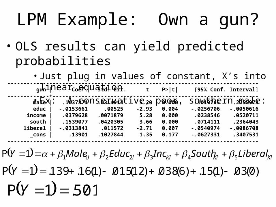
LPM Example: Own a gun?
• OLS results can yield predicted probabilities• Just plug in values of constant, X’s into linear equation• Ex: A conservative, poor, southern male:
------------------------------------------------------------------------------ gun | Coef. Std. Err. t P>|t| [95% Conf. Interval]-------------+---------------------------------------------------------------- male | .1637871 .0314914 5.20 0.000 .1019765 .2255978 educ | -.0153661 .00525 -2.93 0.004 -.0256706 -.0050616 income | .0379628 .0071879 5.28 0.000 .0238546 .0520711 south | .1539077 .0420305 3.66 0.000 .0714111 .2364043 liberal | -.0313841 .011572 -2.71 0.007 -.0540974 -.0086708 _cons | .13901 .1027844 1.35 0.177 -.0627331 .3407531------------------------------------------------------------------------------
KiKiKiii LiberalSouthIncEducMaleY 54322111P
)0(03.)1(15.)6(038.)12(015.)1(16.139.1P Y
501.1P Y
LPM Example: Own a gun?
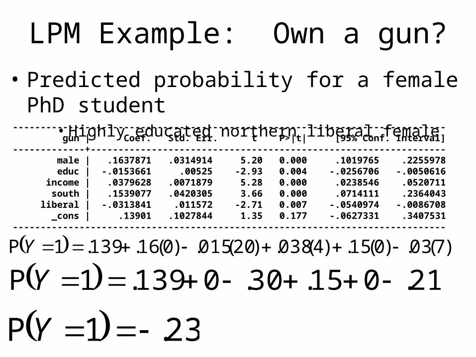
• Predicted probability for a female PhD student• Highly educated northern liberal female
------------------------------------------------------------------------------ gun | Coef. Std. Err. t P>|t| [95% Conf. Interval]-------------+---------------------------------------------------------------- male | .1637871 .0314914 5.20 0.000 .1019765 .2255978 educ | -.0153661 .00525 -2.93 0.004 -.0256706 -.0050616 income | .0379628 .0071879 5.28 0.000 .0238546 .0520711 south | .1539077 .0420305 3.66 0.000 .0714111 .2364043 liberal | -.0313841 .011572 -2.71 0.007 -.0540974 -.0086708 _cons | .13901 .1027844 1.35 0.177 -.0627331 .3407531------------------------------------------------------------------------------
)7(03.)0(15.)4(038.)20(015.)0(16.139.1P Y
23.1P Y
21.015.30.0139.1P Y
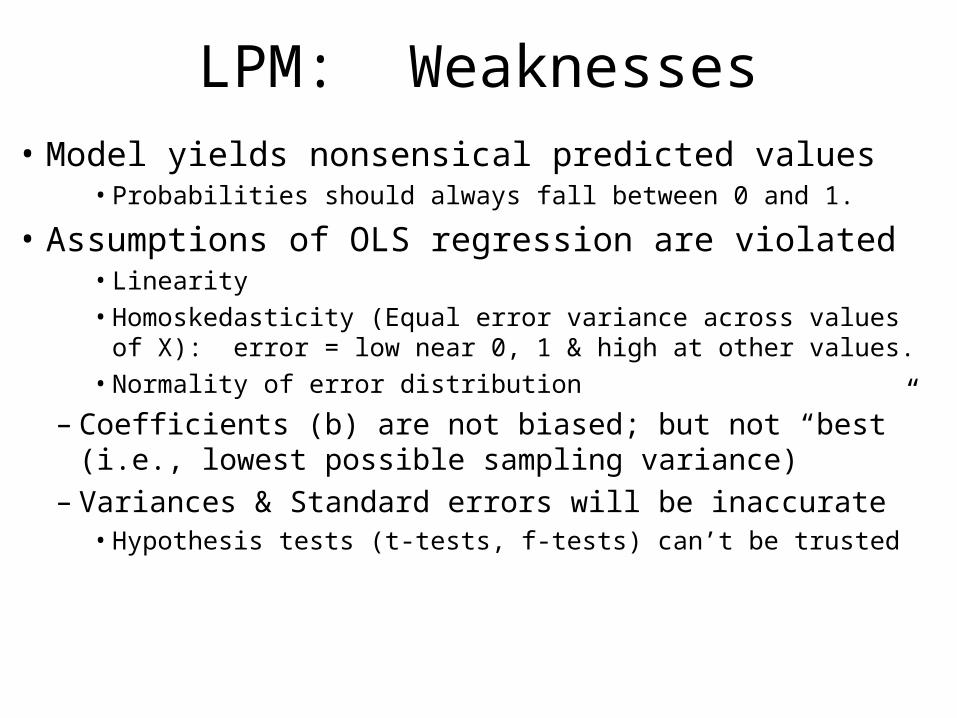
LPM: Weaknesses
• Model yields nonsensical predicted values• Probabilities should always fall between 0 and 1.
• Assumptions of OLS regression are violated• Linearity• Homoskedasticity (Equal error variance across values
of X): error = low near 0, 1 & high at other values. • Normality of error distribution
– Coefficients (b) are not biased; but not “best” (i.e., lowest possible sampling variance)
– Variances & Standard errors will be inaccurate• Hypothesis tests (t-tests, f-tests) can’t be trusted
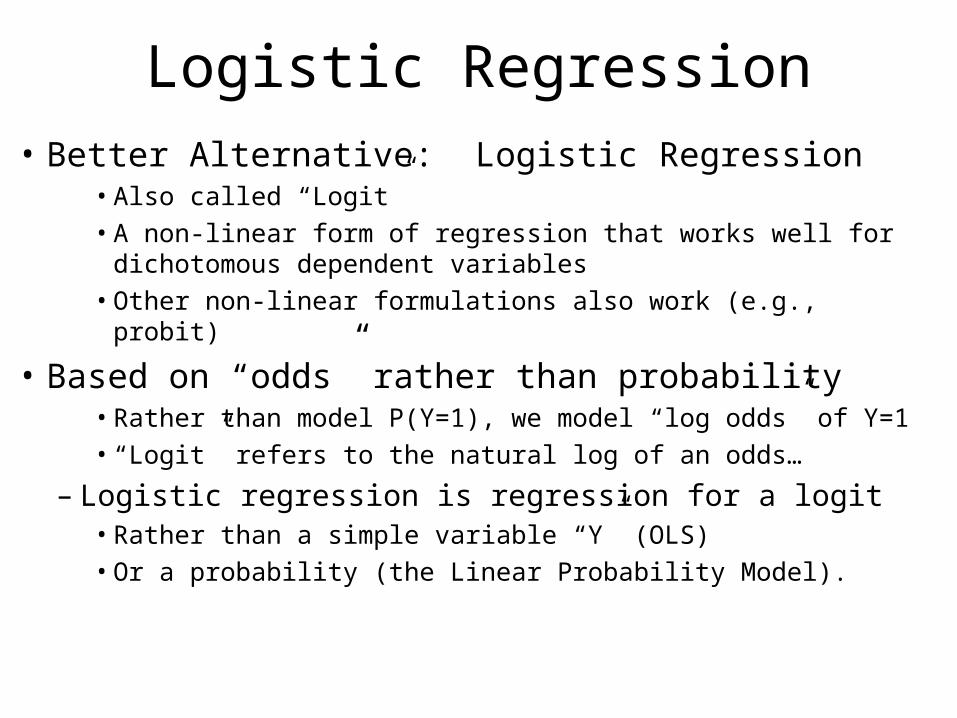
Logistic Regression
• Better Alternative: Logistic Regression• Also called “Logit”• A non-linear form of regression that works well for
dichotomous dependent variables• Other non-linear formulations also work (e.g., probit)
• Based on “odds” rather than probability• Rather than model P(Y=1), we model “log odds” of Y=1• “Logit” refers to the natural log of an odds…
– Logistic regression is regression for a logit• Rather than a simple variable “Y” (OLS)• Or a probability (the Linear Probability Model).
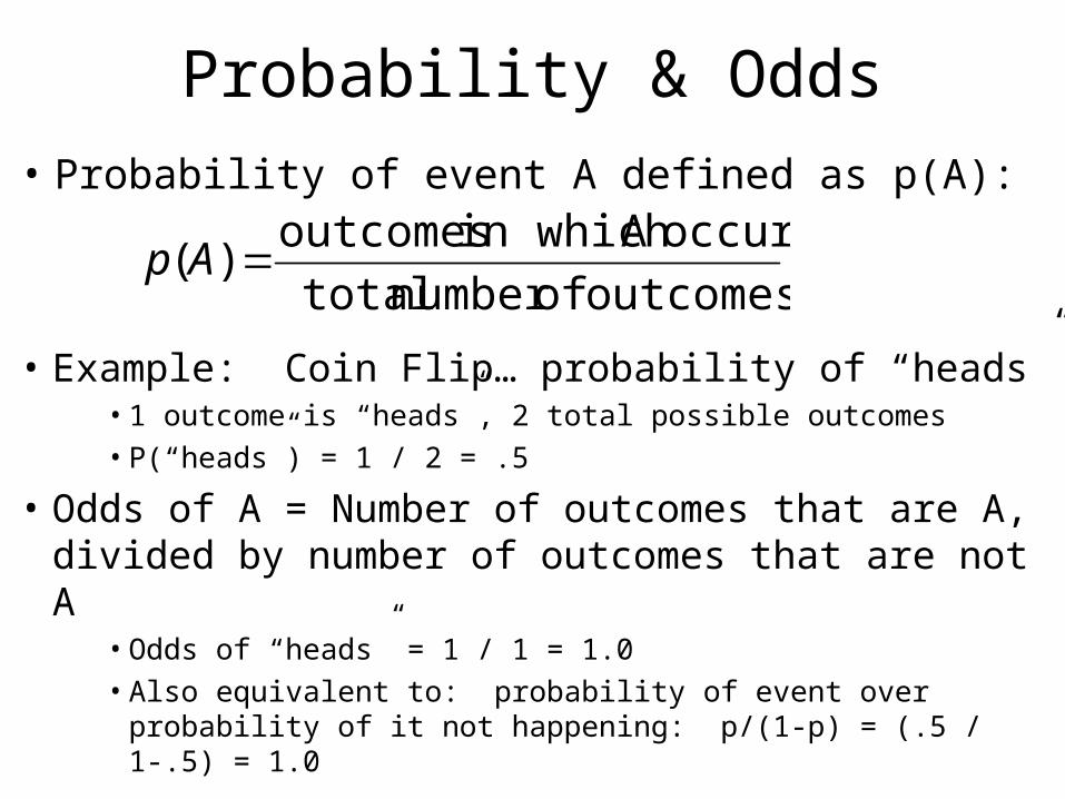
Probability & Odds
• Probability of event A defined as p(A):
outcomes ofnumber total
occursA in which outcomes)( Ap
• Example: Coin Flip… probability of “heads”• 1 outcome is “heads”, 2 total possible outcomes • P(“heads”) = 1 / 2 = .5
• Odds of A = Number of outcomes that are A, divided by number of outcomes that are not A
• Odds of “heads” = 1 / 1 = 1.0• Also equivalent to: probability of event over probability of
it not happening: p/(1-p) = (.5 / 1-.5) = 1.0
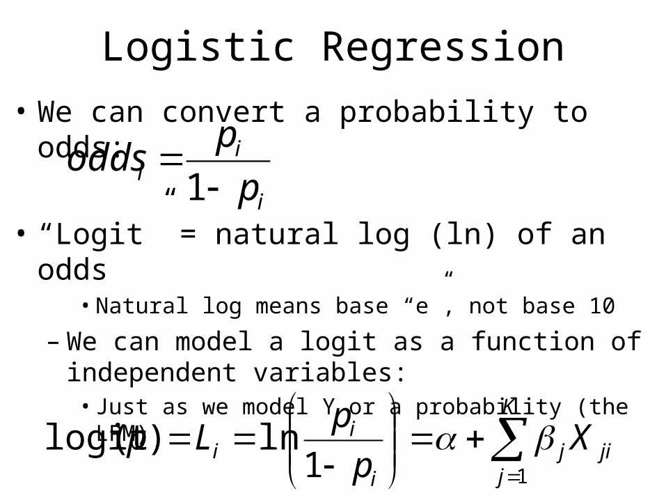
Logistic Regression
• We can convert a probability to odds:
• “Logit” = natural log (ln) of an odds• Natural log means base “e”, not base 10
– We can model a logit as a function of independent variables:
• Just as we model Y or a probability (the LPM)
i
ii p
podds
1
K
jjij
i
ii X
p
pLp
11ln)(logit
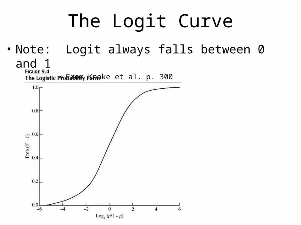
The Logit Curve
• Note: Logit always falls between 0 and 1» From Knoke et al. p. 300

Logistic Regression
• Note: We can solve for “p” and reformulate the model:
ee
eK
jjij
K
jjij
K
jjij
XBXB
XB
YP
11 11
1 1)1(
• Why model this rather than a probability?– Because it is a useful non-linear transformation
• It always generates Ps between 0 and 1, regardless of the values of X variables
• Note: probit transformation has similar effect.
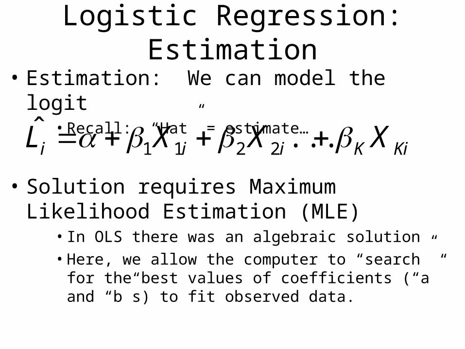
Logistic Regression: Estimation
• Estimation: We can model the logit• Recall: “Hat” = estimate…
KiKiii XXXL ...ˆ2211
• Solution requires Maximum Likelihood Estimation (MLE)
• In OLS there was an algebraic solution• Here, we allow the computer to “search” for the best
values of coefficients (“a” and “b”s) to fit observed data.
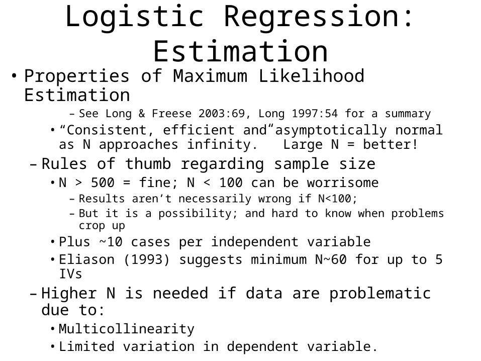
Logistic Regression: Estimation• Properties of Maximum Likelihood Estimation
– See Long & Freese 2003:69, Long 1997:54 for a summary
• “Consistent, efficient and asymptotically normal as N approaches infinity.” Large N = better!
– Rules of thumb regarding sample size• N > 500 = fine; N < 100 can be worrisome
– Results aren’t necessarily wrong if N<100; – But it is a possibility; and hard to know when problems crop up
• Plus ~10 cases per independent variable• Eliason (1993) suggests minimum N~60 for up to 5 IVs
– Higher N is needed if data are problematic due to:• Multicollinearity• Limited variation in dependent variable.
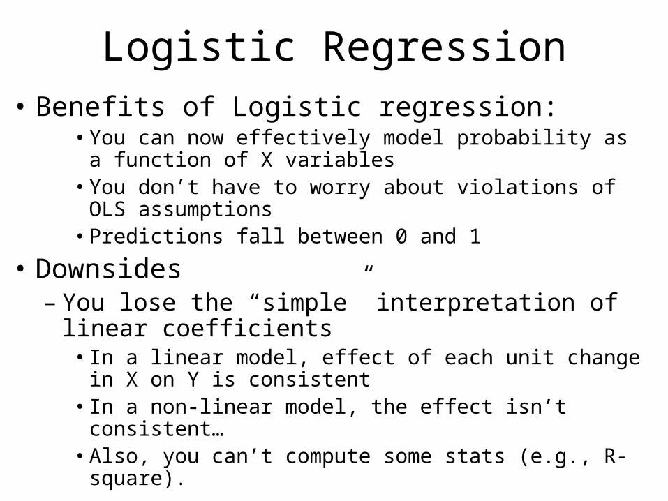
Logistic Regression• Benefits of Logistic regression:
• You can now effectively model probability as a function of X variables
• You don’t have to worry about violations of OLS assumptions
• Predictions fall between 0 and 1
• Downsides– You lose the “simple” interpretation of linear
coefficients• In a linear model, effect of each unit change in X on Y
is consistent• In a non-linear model, the effect isn’t consistent…• Also, you can’t compute some stats (e.g., R-square).
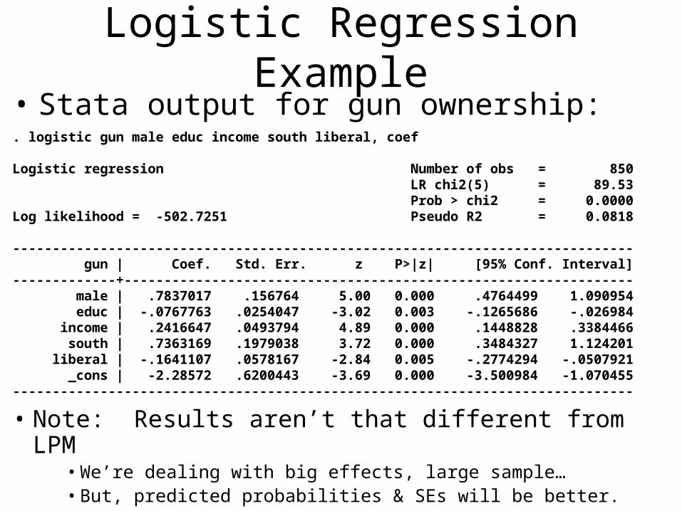
Logistic Regression Example• Stata output for gun ownership:. logistic gun male educ income south liberal, coef
Logistic regression Number of obs = 850 LR chi2(5) = 89.53 Prob > chi2 = 0.0000Log likelihood = -502.7251 Pseudo R2 = 0.0818
------------------------------------------------------------------------------ gun | Coef. Std. Err. z P>|z| [95% Conf. Interval]-------------+---------------------------------------------------------------- male | .7837017 .156764 5.00 0.000 .4764499 1.090954 educ | -.0767763 .0254047 -3.02 0.003 -.1265686 -.026984 income | .2416647 .0493794 4.89 0.000 .1448828 .3384466 south | .7363169 .1979038 3.72 0.000 .3484327 1.124201 liberal | -.1641107 .0578167 -2.84 0.005 -.2774294 -.0507921 _cons | -2.28572 .6200443 -3.69 0.000 -3.500984 -1.070455------------------------------------------------------------------------------
• Note: Results aren’t that different from LPM• We’re dealing with big effects, large sample…• But, predicted probabilities & SEs will be better.
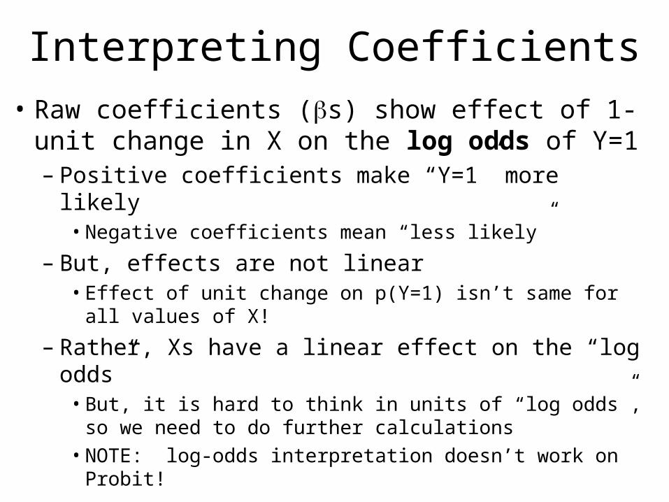
Interpreting Coefficients
• Raw coefficients (s) show effect of 1-unit change in X on the log odds of Y=1– Positive coefficients make “Y=1” more likely
• Negative coefficients mean “less likely”
– But, effects are not linear• Effect of unit change on p(Y=1) isn’t same for all values
of X!
– Rather, Xs have a linear effect on the “log odds”• But, it is hard to think in units of “log odds”, so we need
to do further calculations• NOTE: log-odds interpretation doesn’t work on Probit!
Interpreting Coefficients
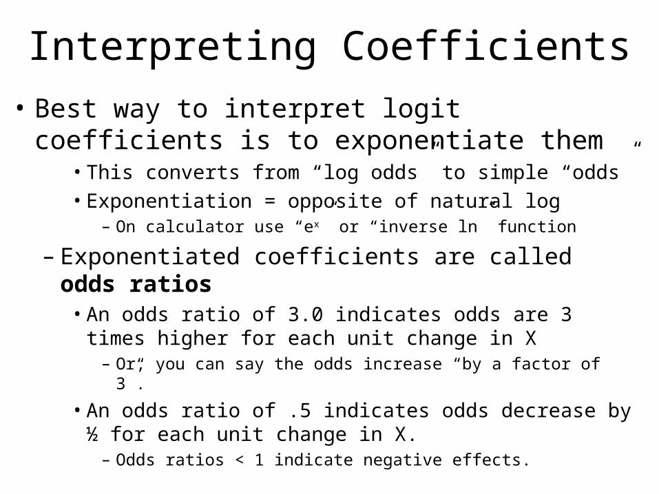
• Best way to interpret logit coefficients is to exponentiate them
• This converts from “log odds” to simple “odds”• Exponentiation = opposite of natural log
– On calculator use “ex” or “inverse ln” function
– Exponentiated coefficients are called odds ratios• An odds ratio of 3.0 indicates odds are 3 times higher
for each unit change in X– Or, you can say the odds increase “by a factor of 3”.
• An odds ratio of .5 indicates odds decrease by ½ for each unit change in X.
– Odds ratios < 1 indicate negative effects.
Interpreting Coefficients
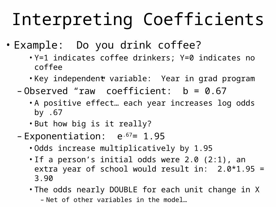
• Example: Do you drink coffee?• Y=1 indicates coffee drinkers; Y=0 indicates no coffee• Key independent variable: Year in grad program
– Observed “raw” coefficient: b = 0.67• A positive effect… each year increases log odds by .67• But how big is it really?
– Exponentiation: e.67= 1.95 • Odds increase multiplicatively by 1.95• If a person’s initial odds were 2.0 (2:1), an extra year of
school would result in: 2.0*1.95 = 3.90• The odds nearly DOUBLE for each unit change in X
– Net of other variables in the model…
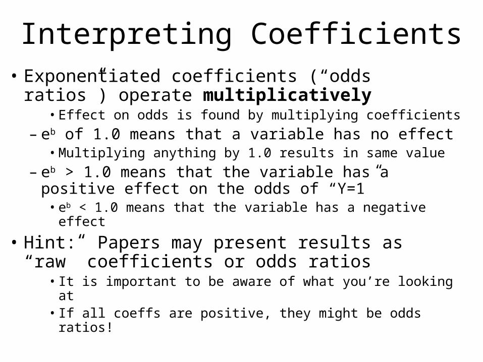
Interpreting Coefficients• Exponentiated coefficients (“odds ratios”)
operate multiplicatively• Effect on odds is found by multiplying coefficients
– eb of 1.0 means that a variable has no effect• Multiplying anything by 1.0 results in same value
– eb > 1.0 means that the variable has a positive effect on the odds of “Y=1”
• eb < 1.0 means that the variable has a negative effect
• Hint: Papers may present results as “raw” coefficients or odds ratios
• It is important to be aware of what you’re looking at• If all coeffs are positive, they might be odds ratios!

Interpreting Coefficients
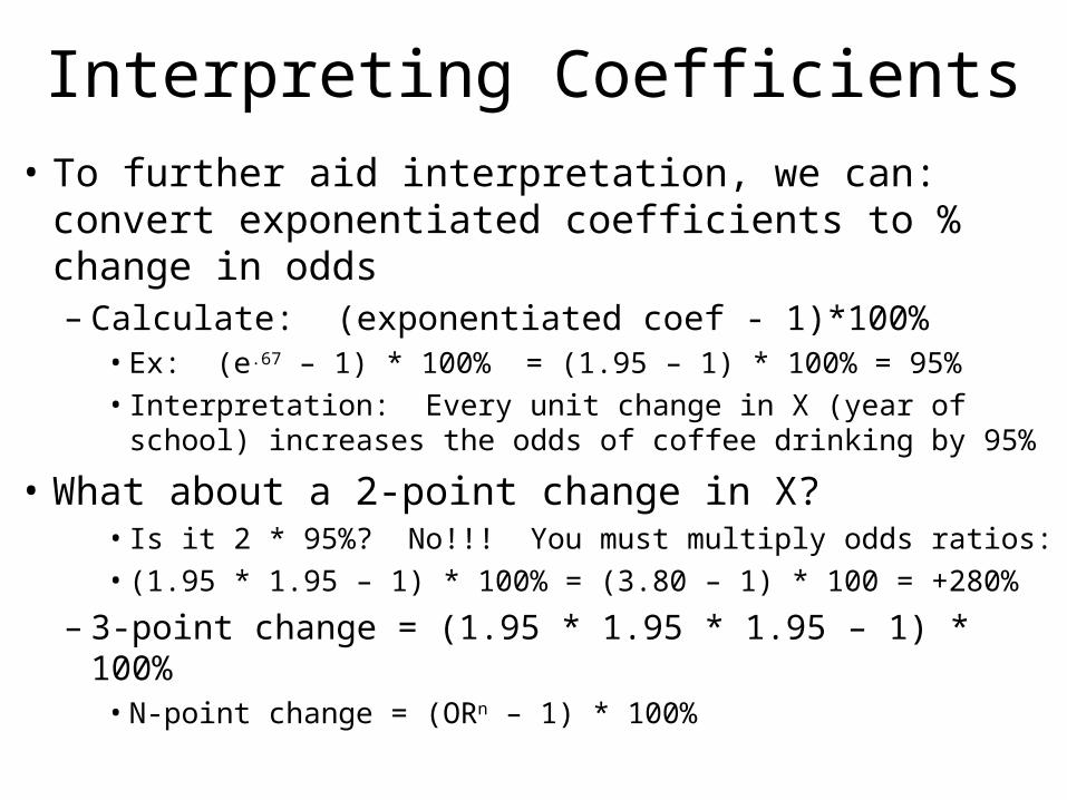
• To further aid interpretation, we can: convert exponentiated coefficients to % change in odds– Calculate: (exponentiated coef - 1)*100%
• Ex: (e.67 – 1) * 100% = (1.95 – 1) * 100% = 95%• Interpretation: Every unit change in X (year of school)
increases the odds of coffee drinking by 95%
• What about a 2-point change in X?• Is it 2 * 95%? No!!! You must multiply odds ratios:• (1.95 * 1.95 – 1) * 100% = (3.80 – 1) * 100 = +280%
– 3-point change = (1.95 * 1.95 * 1.95 – 1) * 100%• N-point change = (ORn – 1) * 100%
Interpreting Coefficients
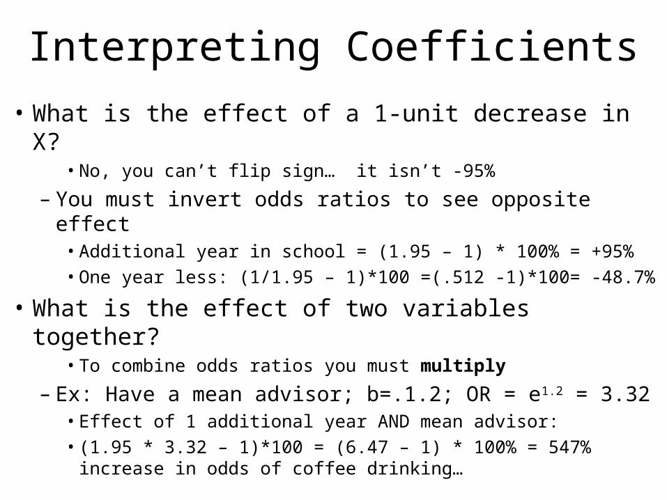
• What is the effect of a 1-unit decrease in X?• No, you can’t flip sign… it isn’t -95%
– You must invert odds ratios to see opposite effect• Additional year in school = (1.95 – 1) * 100% = +95%• One year less: (1/1.95 – 1)*100 =(.512 -1)*100= -48.7%
• What is the effect of two variables together?• To combine odds ratios you must multiply
– Ex: Have a mean advisor; b=.1.2; OR = e1.2 = 3.32• Effect of 1 additional year AND mean advisor:• (1.95 * 3.32 – 1)*100 = (6.47 – 1) * 100% = 547%
increase in odds of coffee drinking…
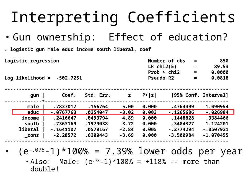
Interpreting Coefficients• Gun ownership: Effect of education?. logistic gun male educ income south liberal, coef
Logistic regression Number of obs = 850 LR chi2(5) = 89.53 Prob > chi2 = 0.0000Log likelihood = -502.7251 Pseudo R2 = 0.0818
------------------------------------------------------------------------------ gun | Coef. Std. Err. z P>|z| [95% Conf. Interval]-------------+---------------------------------------------------------------- male | .7837017 .156764 5.00 0.000 .4764499 1.090954 educ | -.0767763 .0254047 -3.02 0.003 -.1265686 -.026984 income | .2416647 .0493794 4.89 0.000 .1448828 .3384466 south | .7363169 .1979038 3.72 0.000 .3484327 1.124201 liberal | -.1641107 .0578167 -2.84 0.005 -.2774294 -.0507921 _cons | -2.28572 .6200443 -3.69 0.000 -3.500984 -1.070455------------------------------------------------------------------------------
• (e-.076-1)*100% = 7.39% lower odds per year• Also: Male: (e.78-1)*100% = +118% -- more than double!

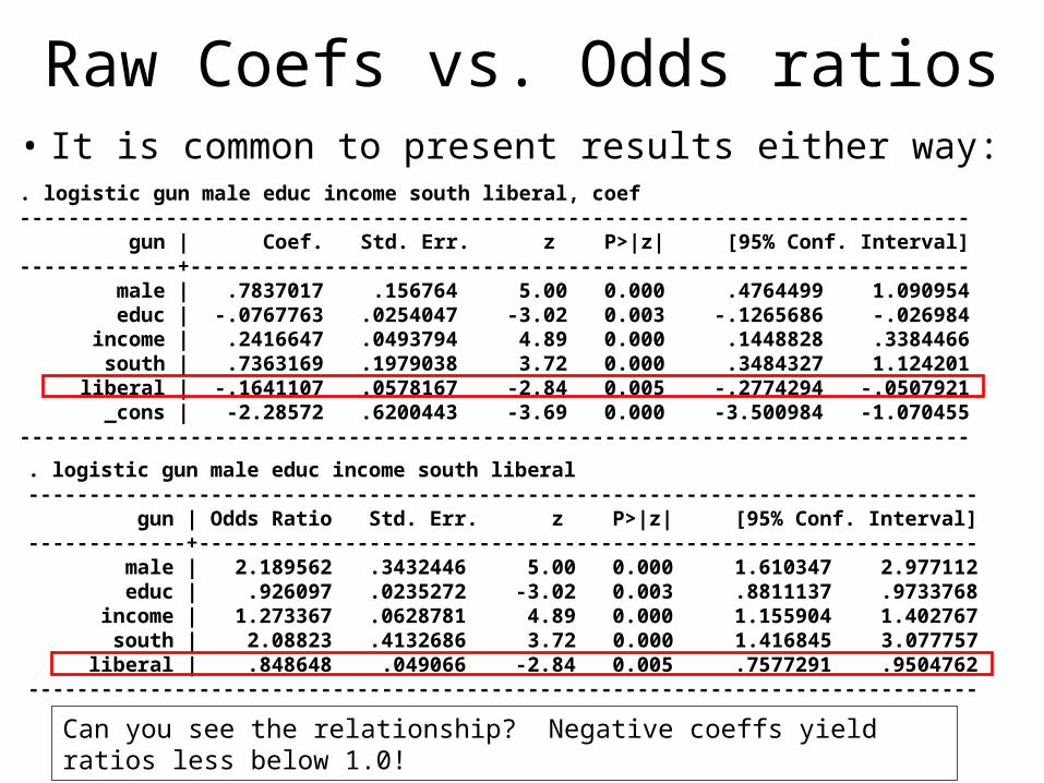
Raw Coefs vs. Odds ratios• It is common to present results either way:. logistic gun male educ income south liberal, coef------------------------------------------------------------------------------ gun | Coef. Std. Err. z P>|z| [95% Conf. Interval]-------------+---------------------------------------------------------------- male | .7837017 .156764 5.00 0.000 .4764499 1.090954 educ | -.0767763 .0254047 -3.02 0.003 -.1265686 -.026984 income | .2416647 .0493794 4.89 0.000 .1448828 .3384466 south | .7363169 .1979038 3.72 0.000 .3484327 1.124201 liberal | -.1641107 .0578167 -2.84 0.005 -.2774294 -.0507921 _cons | -2.28572 .6200443 -3.69 0.000 -3.500984 -1.070455------------------------------------------------------------------------------
. logistic gun male educ income south liberal------------------------------------------------------------------------------ gun | Odds Ratio Std. Err. z P>|z| [95% Conf. Interval]-------------+---------------------------------------------------------------- male | 2.189562 .3432446 5.00 0.000 1.610347 2.977112 educ | .926097 .0235272 -3.02 0.003 .8811137 .9733768 income | 1.273367 .0628781 4.89 0.000 1.155904 1.402767 south | 2.08823 .4132686 3.72 0.000 1.416845 3.077757 liberal | .848648 .049066 -2.84 0.005 .7577291 .9504762------------------------------------------------------------------------------
Can you see the relationship? Negative coeffs yield ratios less below 1.0!

Interpreting Coefficients
• Raw coefficients (s) show effect of 1-unit change in X on the log odds of Y=1– Positive coefficients make “Y=1” more likely
• Negative coefficients mean “less likely”
– But, effects are not linear• Effect of unit change on p(Y=1) isn’t same for all values
of X!
– Rather, Xs have a linear effect on the “log odds”• But, it is hard to think in units of “log odds”, so we need
to do further calculations• NOTE: log-odds interpretation doesn’t work on Probit!

Interpreting Coefficients
• Best way to interpret logit coefficients is to exponentiate them
• This converts from “log odds” to simple “odds”• Exponentiation = opposite of natural log
– On calculator use “ex” or “inverse ln” function
– Exponentiated coefficients are called odds ratios• An odds ratio of 3.0 indicates odds are 3 times higher
for each unit change in X– Or, you can say the odds increase “by a factor of 3”.
• An odds ratio of .5 indicates odds decrease by ½ for each unit change in X.
– Odds ratios < 1 indicate negative effects.
Raw Coefs vs. Odds ratios• It is common to present results either way:. logistic gun male educ income south liberal, coef------------------------------------------------------------------------------ gun | Coef. Std. Err. z P>|z| [95% Conf. Interval]-------------+---------------------------------------------------------------- male | .7837017 .156764 5.00 0.000 .4764499 1.090954 educ | -.0767763 .0254047 -3.02 0.003 -.1265686 -.026984 income | .2416647 .0493794 4.89 0.000 .1448828 .3384466 south | .7363169 .1979038 3.72 0.000 .3484327 1.124201 liberal | -.1641107 .0578167 -2.84 0.005 -.2774294 -.0507921 _cons | -2.28572 .6200443 -3.69 0.000 -3.500984 -1.070455------------------------------------------------------------------------------
. logistic gun male educ income south liberal------------------------------------------------------------------------------ gun | Odds Ratio Std. Err. z P>|z| [95% Conf. Interval]-------------+---------------------------------------------------------------- male | 2.189562 .3432446 5.00 0.000 1.610347 2.977112 educ | .926097 .0235272 -3.02 0.003 .8811137 .9733768 income | 1.273367 .0628781 4.89 0.000 1.155904 1.402767 south | 2.08823 .4132686 3.72 0.000 1.416845 3.077757 liberal | .848648 .049066 -2.84 0.005 .7577291 .9504762------------------------------------------------------------------------------
Can you see the relationship? Negative coeffs yield ratios less below 1.0!

Interpreting Coefficients
• Example: Do you drink coffee?• Y=1 indicates coffee drinkers; Y=0 indicates no coffee• Key independent variable: Year in grad program
– Observed “raw” coefficient: b = 0.67• A positive effect… each year increases log odds by .67• But how big is it really?
– Exponentiation: e.67= 1.95 • Odds increase multiplicatively by 1.95• If a person’s initial odds were 2.0 (2:1), an extra year of
school would result in: 2.0*1.95 = 3.90• The odds nearly DOUBLE for each unit change in X
– Net of other variables in the model…

Interpreting Coefficients• Exponentiated coefficients (“odds ratios”)
operate multiplicatively• Effect on odds is found by multiplying coefficients
– eb of 1.0 means that a variable has no effect• Multiplying anything by 1.0 results in same value
– eb > 1.0 means that the variable has a positive effect on the odds of “Y=1”
• eb < 1.0 means that the variable has a negative effect
• Hint: Papers may present results as “raw” coefficients or odds ratios
• It is important to be aware of what you’re looking at• If all numbers are positive, it is probably odds ratios!
Interpreting Coefficients
• To further aid interpretation, we can: convert exponentiated coefficients to % change in odds– Calculate: (exponentiated coef - 1)*100%
• Ex: (e.67 – 1) * 100% = (1.95 – 1) * 100% = 95%• Interpretation: Every unit change in X (year of school)
increases the odds of coffee drinking by 95%
• What about a 2-point change in X?• Is it 2 * 95%? No!!! You must multiply odds ratios:• (1.95 * 1.95 – 1) * 100% = (3.80 – 1) * 100 = +280%
– 3-point change = (1.95 * 1.95 * 1.95 – 1) * 100%• N-point change = (ORn – 1) * 100%

Interpreting Coefficients
• What is the effect of a 1-unit decrease in X?• No, you can’t flip sign… it isn’t -95%
– You must invert odds ratios to see opposite effect• Additional year in school = (1.95 – 1) * 100% = +95%• One year less: (1/1.95 – 1)*100 =(.512 -1)*100= -48.7%
• What is the effect of two variables together?• To combine odds ratios you must multiply
– Ex: Have a mean advisor; b=.1.2; OR = e1.2 = 3.32• Effect of 1 additional year AND mean advisor:• (1.95 * 3.32 – 1)*100 = (6.47 – 1) * 100% = 547%
increase in odds of coffee drinking…
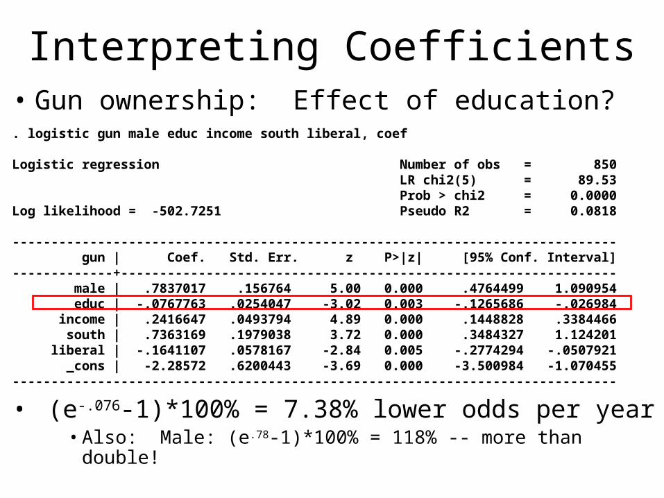
Interpreting Coefficients• Gun ownership: Effect of education?. logistic gun male educ income south liberal, coef
Logistic regression Number of obs = 850 LR chi2(5) = 89.53 Prob > chi2 = 0.0000Log likelihood = -502.7251 Pseudo R2 = 0.0818
------------------------------------------------------------------------------ gun | Coef. Std. Err. z P>|z| [95% Conf. Interval]-------------+---------------------------------------------------------------- male | .7837017 .156764 5.00 0.000 .4764499 1.090954 educ | -.0767763 .0254047 -3.02 0.003 -.1265686 -.026984 income | .2416647 .0493794 4.89 0.000 .1448828 .3384466 south | .7363169 .1979038 3.72 0.000 .3484327 1.124201 liberal | -.1641107 .0578167 -2.84 0.005 -.2774294 -.0507921 _cons | -2.28572 .6200443 -3.69 0.000 -3.500984 -1.070455------------------------------------------------------------------------------
• (e-.076-1)*100% = 7.38% lower odds per year• Also: Male: (e.78-1)*100% = 118% -- more than double!
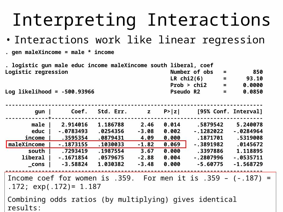
Interpreting Interactions• Interactions work like linear regression. gen maleXincome = male * income
. logistic gun male educ income maleXincome south liberal, coefLogistic regression Number of obs = 850 LR chi2(6) = 93.10 Prob > chi2 = 0.0000Log likelihood = -500.93966 Pseudo R2 = 0.0850
------------------------------------------------------------------------------ gun | Coef. Std. Err. z P>|z| [95% Conf. Interval]-------------+---------------------------------------------------------------- male | 2.914016 1.186788 2.46 0.014 .5879542 5.240078 educ | -.0783493 .0254356 -3.08 0.002 -.1282022 -.0284964 income | .3595354 .0879431 4.09 0.000 .1871701 .5319008 maleXincome | -.1873155 .1030033 -1.82 0.069 -.3891982 .0145672 south | .7293419 .1987554 3.67 0.000 .3397886 1.118895 liberal | -.1671854 .0579675 -2.88 0.004 -.2807996 -.0535711 _cons | -3.58824 1.030382 -3.48 0.000 -5.60775 -1.568729------------------------------------------------------------------------------Income coef for women is .359. For men it is .359 – (-.187) = .172; exp(.172)= 1.187
Combining odds ratios (by multiplying) gives identical results:
exp(.359) * exp (-.187) = 1.43 * .083 = 1.187
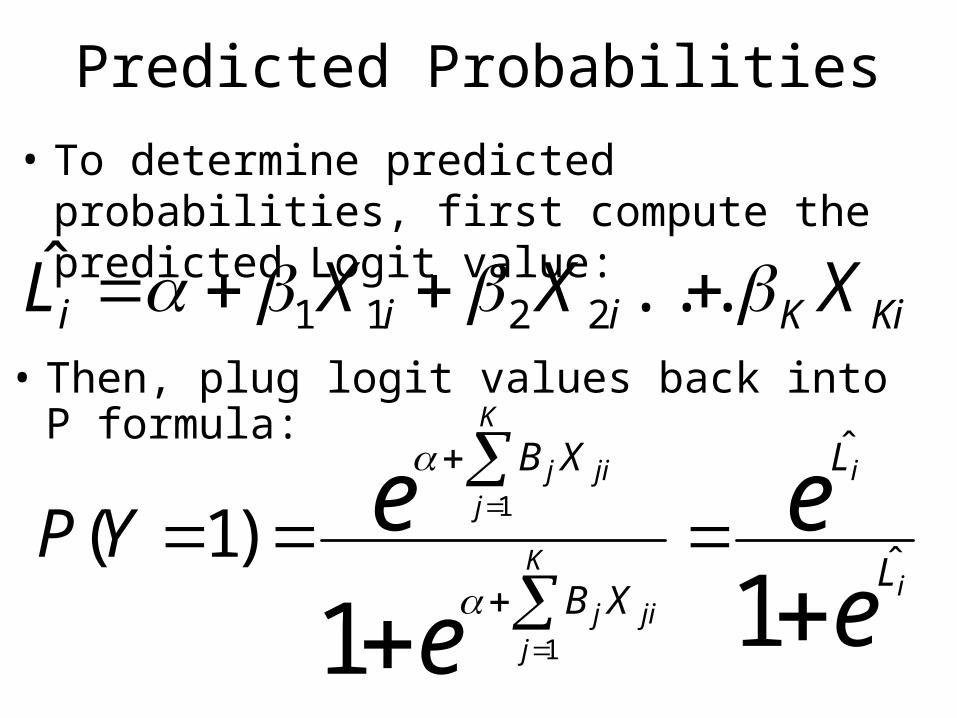
Predicted Probabilities
• To determine predicted probabilities, first compute the predicted Logit value:
KiKiii XXXL ...ˆ2211
ee
e
ei
i
K
jjij
K
jjij
L
L
XB
XB
YP
11ˆ
ˆ
1
1
)1(
• Then, plug logit values back into P formula:
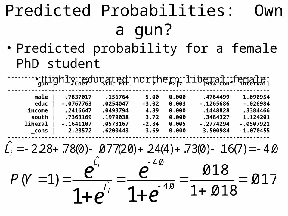
Predicted Probabilities: Own a gun?
• Predicted probability for a female PhD student• Highly educated northern liberal female
------------------------------------------------------------------------------ gun | Coef. Std. Err. z P>|z| [95% Conf. Interval]-------------+---------------------------------------------------------------- male | .7837017 .156764 5.00 0.000 .4764499 1.090954 educ | -.0767763 .0254047 -3.02 0.003 -.1265686 -.026984 income | .2416647 .0493794 4.89 0.000 .1448828 .3384466 south | .7363169 .1979038 3.72 0.000 .3484327 1.124201 liberal | -.1641107 .0578167 -2.84 0.005 -.2774294 -.0507921 _cons | -2.28572 .6200443 -3.69 0.000 -3.500984 -1.070455------------------------------------------------------------------------------
0.4)7(16.)0(73.)4(24.)20(077.)0(78.28.2ˆ iL
017.018.1
018.)1(
110.4
0.4
ˆ
ˆ
ee
ee
i
i
L
L
YP
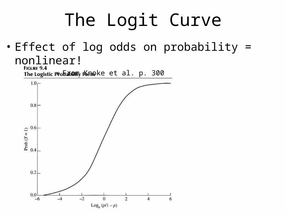
The Logit Curve
• Effect of log odds on probability = nonlinear!» From Knoke et al. p. 300
Predicted Probabilities
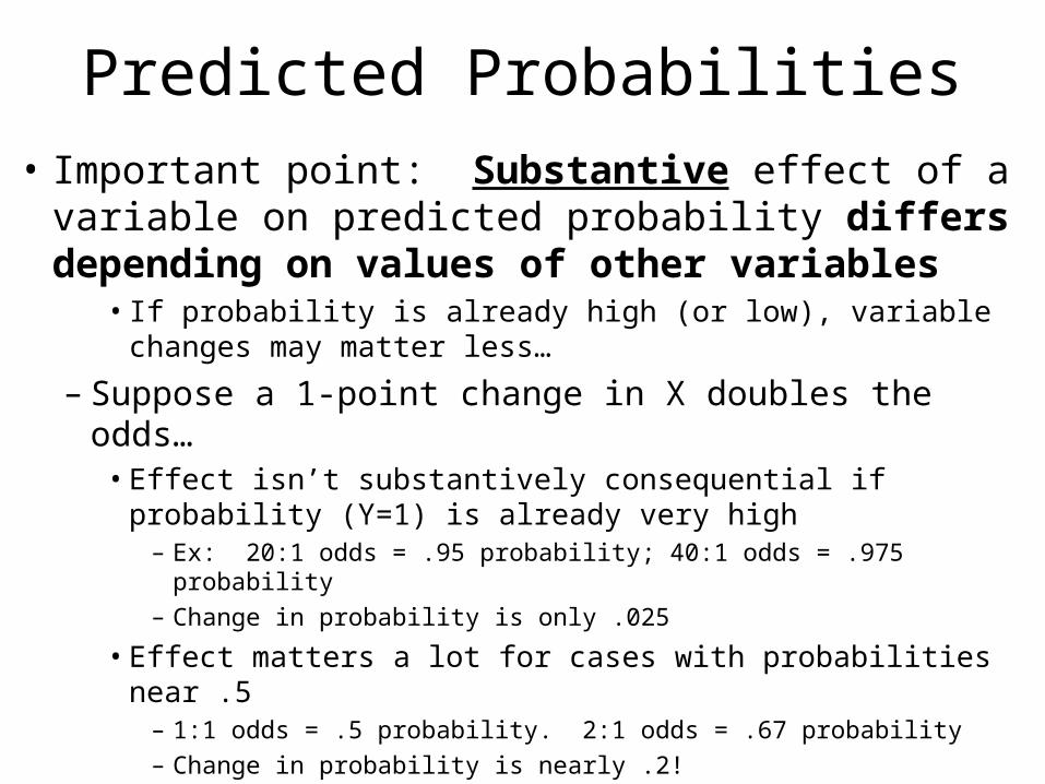
• Important point: Substantive effect of a variable on predicted probability differs depending on values of other variables
• If probability is already high (or low), variable changes may matter less…
– Suppose a 1-point change in X doubles the odds…• Effect isn’t substantively consequential if probability
(Y=1) is already very high– Ex: 20:1 odds = .95 probability; 40:1 odds = .975 probability– Change in probability is only .025
• Effect matters a lot for cases with probabilities near .5– 1:1 odds = .5 probability. 2:1 odds = .67 probability– Change in probability is nearly .2!
Logit Example: Own a gun?
• Predicted probability of gun ownership for a female PhD student is very low: P=.017– Two additional years of education lowers
probability from .017 to .015 – not a big effect• Additional unit change can’t have a big effect –
because probability can’t go below zero • It would matter much more for a southern male…
16.4)7(16.)0(73.)4(24.)22(077.)0(78.28.2ˆ iL
0153.0156.1
0156.)1(
110.4
0.4
ˆ
ˆ
ee
ee
i
i
L
L
YP
Predicted Probabilities
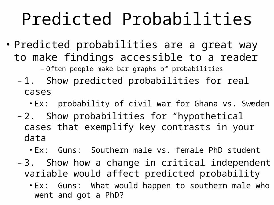
• Predicted probabilities are a great way to make findings accessible to a reader
– Often people make bar graphs of probabilities
– 1. Show predicted probabilities for real cases• Ex: probability of civil war for Ghana vs. Sweden
– 2. Show probabilities for “hypothetical” cases that exemplify key contrasts in your data
• Ex: Guns: Southern male vs. female PhD student
– 3. Show how a change in critical independent variable would affect predicted probability
• Ex: Guns: What would happen to southern male who went and got a PhD?

Predicted Probabilities: Stata
• Like OLS regression, we can calculate predicted values for all cases
. predict predprob, pr(1488 missing values generated)
. list predprob gun if gun ~= .
+----------------+ | predprob gun | |----------------| 1. | .486874 0 | 2. | .6405225 1 | 6. | .7078031 1 | 9. | .6750654 1 | 14. | .4243994 0 | |----------------| 17. | .0617232 0 | 19. | .6556235 1 | 22. | .6356462 0 | 27. | .3670604 0 | 32. | .5620316 0 |
Many of the predictions are pretty good
But, some aren’t!
Predicted Probabilities: Stata
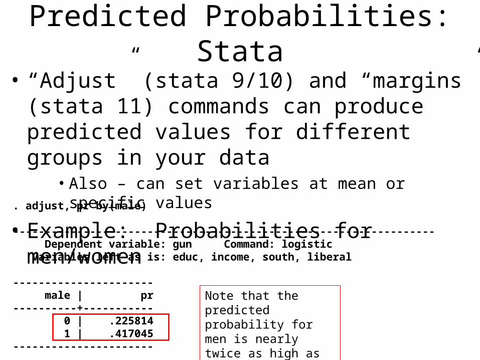
• “Adjust” (stata 9/10) and “margins” (stata 11) commands can produce predicted values for different groups in your data
• Also – can set variables at mean or specific values
• Example: Probabilities for men/women. adjust, pr by(male)
------------------------------------------------------------------ Dependent variable: gun Command: logistic Variables left as is: educ, income, south, liberal
---------------------- male | pr----------+----------- 0 | .225814 1 | .417045----------------------
Note that the predicted probability for men is nearly twice as high as for women.

Stata Notes: Adjust Command
• Stata “adjust” command can be tricky– 1. By default it uses the entire sample, not just
cases in your prior analysis• Best to specify prior sample: • adjust if e(sample), pr by(male)
– 2. For non-specified variables, stata uses group means (defined by “by” command)
• Don’t assume it pegs cases to overall sample mean• Variables “left as is” take on mean for subgroups
– 3. It doesn’t take into account weighted data• Use “lincom” if you have weighted data
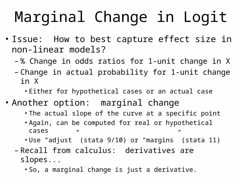
Marginal Change in Logit
• Issue: How to best capture effect size in non-linear models?– % Change in odds ratios for 1-unit change in X– Change in actual probability for 1-unit change in X
• Either for hypothetical cases or an actual case
• Another option: marginal change• The actual slope of the curve at a specific point• Again, can be computed for real or hypothetical cases• Use “adjust” (stata 9/10) or “margins” (stata 11)
– Recall from calculus: derivatives are slopes...• So, a marginal change is just a derivative.
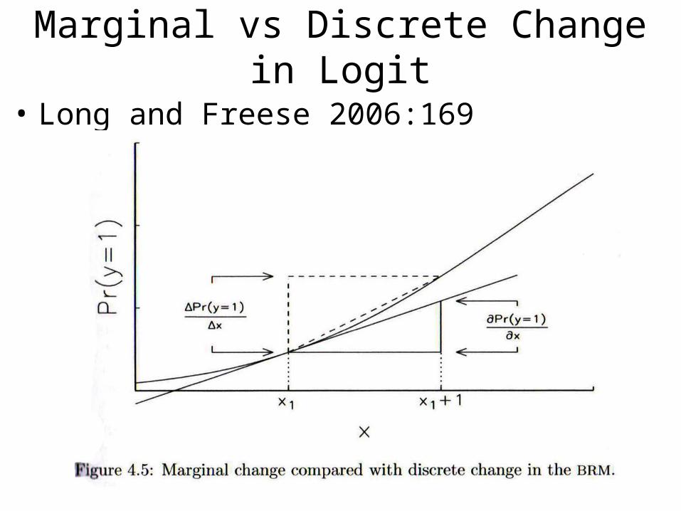
Marginal vs Discrete Change in Logit
• Long and Freese 2006:169
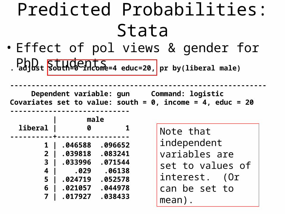
Predicted Probabilities: Stata
• Effect of pol views & gender for PhD students
. adjust south=0 income=4 educ=20, pr by(liberal male)
------------------------------------------------------------ Dependent variable: gun Command: logisticCovariates set to value: south = 0, income = 4, educ = 20---------------------------- | male liberal | 0 1----------+----------------- 1 | .046588 .096652 2 | .039818 .083241 3 | .033996 .071544 4 | .029 .06138 5 | .024719 .052578 6 | .021057 .044978 7 | .017927 .038433
Note that independent variables are set to values of interest. (Or can be set to mean).
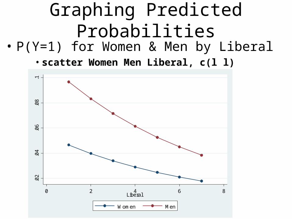
Graphing Predicted Probabilities• P(Y=1) for Women & Men by Liberal
• scatter Women Men Liberal, c(l l)
.02
.04
.06
.08
.1
0 2 4 6 8Liberal
Women Men
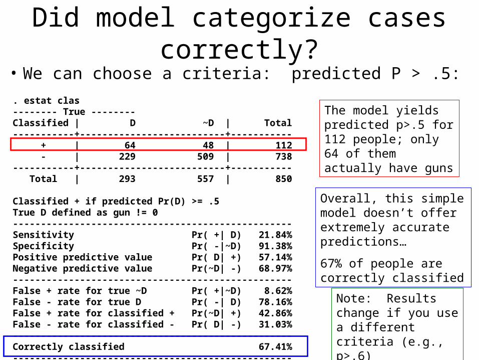
Did model categorize cases correctly?
• We can choose a criteria: predicted P > .5:. estat clas-------- True --------Classified | D ~D | Total-----------+--------------------------+----------- + | 64 48 | 112 - | 229 509 | 738-----------+--------------------------+----------- Total | 293 557 | 850
Classified + if predicted Pr(D) >= .5True D defined as gun != 0--------------------------------------------------Sensitivity Pr( +| D) 21.84%Specificity Pr( -|~D) 91.38%Positive predictive value Pr( D| +) 57.14%Negative predictive value Pr(~D| -) 68.97%--------------------------------------------------False + rate for true ~D Pr( +|~D) 8.62%False - rate for true D Pr( -| D) 78.16%False + rate for classified + Pr(~D| +) 42.86%False - rate for classified - Pr( D| -) 31.03%--------------------------------------------------Correctly classified 67.41%--------------------------------------------------
The model yields predicted p>.5 for 112 people; only 64 of them actually have guns
Overall, this simple model doesn’t offer extremely accurate predictions…
67% of people are correctly classified
Note: Results change if you use a different criteria (e.g., p>.6)
Sensitivity / Specificity of Prediction
• Sensitivity: Of gun owners, what proportion were correctly predicted to own a gun?
• Specificity: Of non-gun owners, what proportion did we correctly predict?
• Choosing a different probability cutoff affects those values
• If we reduce the cutoff to P > .4, we’ll catch a higher proportion of gun owners
• But, we’ll incorrectly identify more non-gun owners.• And, we’ll have more false positives.
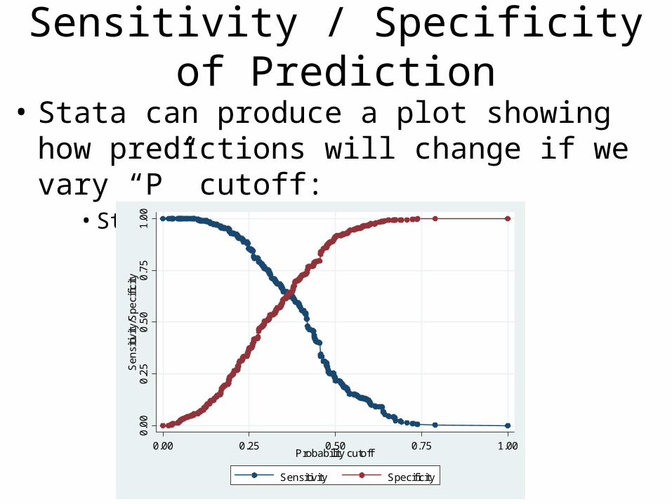
Sensitivity / Specificity of Prediction
• Stata can produce a plot showing how predictions will change if we vary “P” cutoff:
• Stata command: lsens
0.0
00.
25
0.5
00.
75
1.0
0S
ensi
tivity
/Spe
cific
ity
0.00 0.25 0.50 0.75 1.00Probability cutoff
Sensitivity Specificity
Hypothesis tests
• Testing hypotheses using logistic regression• H0: There is no effect of year in grad program on coffee
drinking• H1: Year in grad school is associated with coffee
– Or, one-tail test: Year in school increases probability of coffee
– MLE estimation yields standard errors… like OLS– Test statistic: 2 options; both yield same results
• t = b/SE… just like OLS regression • Wald test (Chi-square, 1df); essentially the square of t
– Reject H0 if Wald or t > critical value• Or if p-value less than alpha (usually .05).
Model Fit: Likelihood Ratio Tests
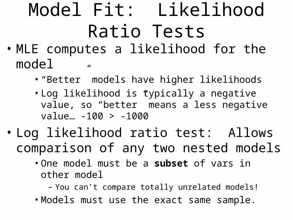
• MLE computes a likelihood for the model• “Better” models have higher likelihoods• Log likelihood is typically a negative value, so “better”
means a less negative value… -100 > -1000
• Log likelihood ratio test: Allows comparison of any two nested models
• One model must be a subset of vars in other model– You can’t compare totally unrelated models!
• Models must use the exact same sample.
Model Fit: Likelihood Ratio Tests
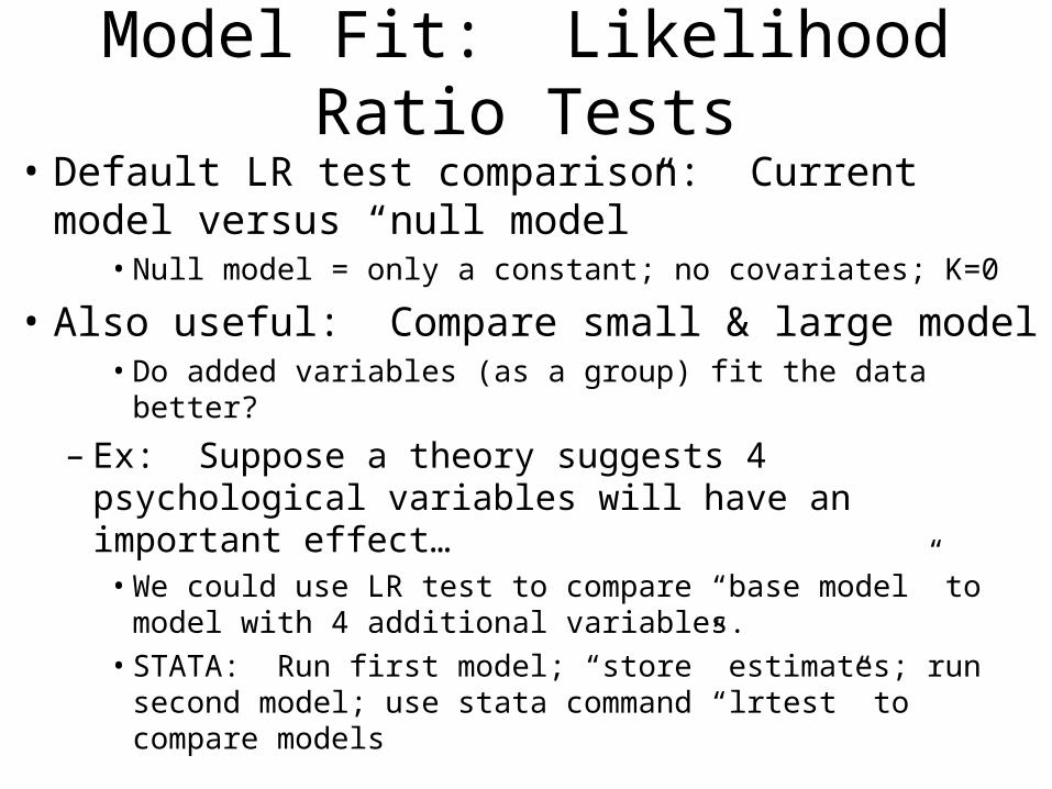
• Default LR test comparison: Current model versus “null model”
• Null model = only a constant; no covariates; K=0
• Also useful: Compare small & large model• Do added variables (as a group) fit the data better?
– Ex: Suppose a theory suggests 4 psychological variables will have an important effect…
• We could use LR test to compare “base model” to model with 4 additional variables.
• STATA: Run first model; “store” estimates; run second model; use stata command “lrtest” to compare models
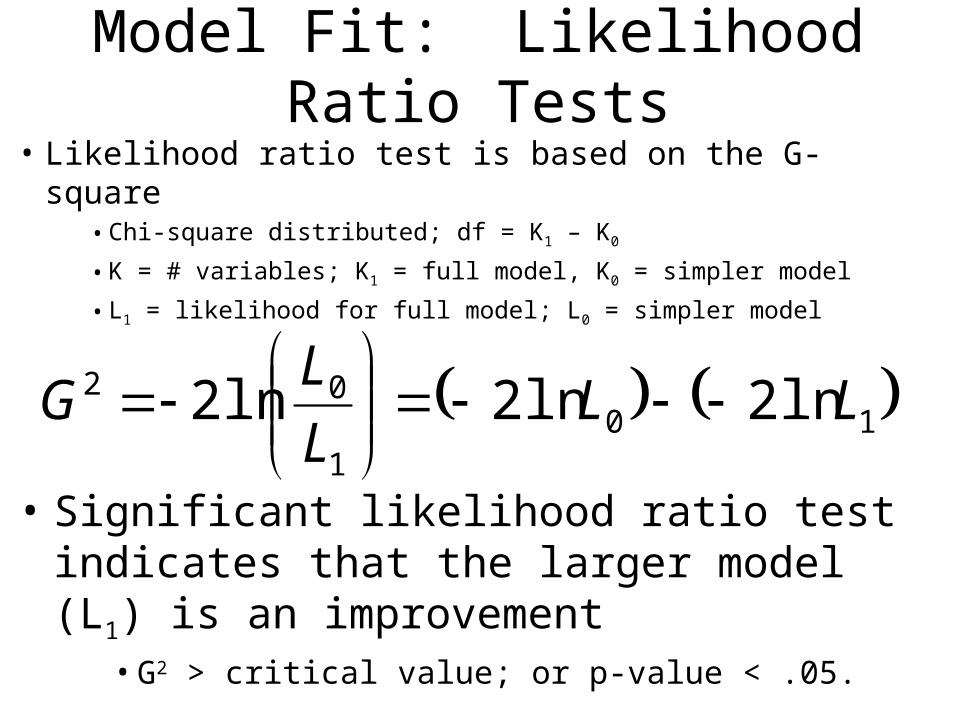
Model Fit: Likelihood Ratio Tests
• Likelihood ratio test is based on the G-square• Chi-square distributed; df = K1 – K0
• K = # variables; K1 = full model, K0 = simpler model
• L1 = likelihood for full model; L0 = simpler model
101
02 ln2ln2ln2 LLL
LG
• Significant likelihood ratio test indicates that the larger model (L1) is an improvement
• G2 > critical value; or p-value < .05.

Model Fit: Likelihood Ratio Tests• Stata’s default LR test; compares to null model. logistic gun male educ income south liberal, coef
Logistic regression Number of obs = 850 LR chi2(5) = 89.53 Prob > chi2 = 0.0000Log likelihood = -502.7251 Pseudo R2 = 0.0818
------------------------------------------------------------------------------ gun | Coef. Std. Err. z P>|z| [95% Conf. Interval]-------------+---------------------------------------------------------------- male | .7837017 .156764 5.00 0.000 .4764499 1.090954 educ | -.0767763 .0254047 -3.02 0.003 -.1265686 -.026984 income | .2416647 .0493794 4.89 0.000 .1448828 .3384466 south | .7363169 .1979038 3.72 0.000 .3484327 1.124201 liberal | -.1641107 .0578167 -2.84 0.005 -.2774294 -.0507921 _cons | -2.28572 .6200443 -3.69 0.000 -3.500984 -1.070455------------------------------------------------------------------------------
LR Chi2(5) indicates G-square for 5 degrees of freedom
Prob > chi2 is a p-value. p < .05 indicates a significantly better model
Model likelihood = -502.7 Null model is a lower value (more negative)
Model Fit: Likelihood Ratio Tests
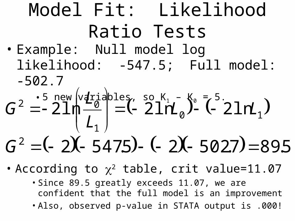
• Example: Null model log likelihood: -547.5; Full model: -502.7
• 5 new variables, so K1 – K0 = 5.
101
02 ln2ln2ln2 LLL
LG
• According to 2 table, crit value=11.07• Since 89.5 greatly exceeds 11.07, we are confident that
the full model is an improvement• Also, observed p-value in STATA output is .000!
5.897.50225.54722 G
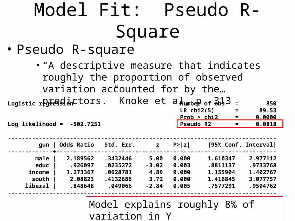
Model Fit: Pseudo R-Square
• Pseudo R-square• “A descriptive measure that indicates roughly the
proportion of observed variation accounted for by the… predictors.” Knoke et al, p. 313
Logistic regression Number of obs = 850 LR chi2(5) = 89.53 Prob > chi2 = 0.0000Log likelihood = -502.7251 Pseudo R2 = 0.0818
------------------------------------------------------------------------------ gun | Odds Ratio Std. Err. z P>|z| [95% Conf. Interval]-------------+---------------------------------------------------------------- male | 2.189562 .3432446 5.00 0.000 1.610347 2.977112 educ | .926097 .0235272 -3.02 0.003 .8811137 .9733768 income | 1.273367 .0628781 4.89 0.000 1.155904 1.402767 south | 2.08823 .4132686 3.72 0.000 1.416845 3.077757 liberal | .848648 .049066 -2.84 0.005 .7577291 .9504762------------------------------------------------------------------------------
Model explains roughly 8% of variation in Y
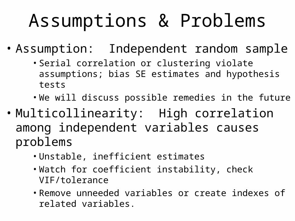
Assumptions & Problems
• Assumption: Independent random sample• Serial correlation or clustering violate assumptions; bias
SE estimates and hypothesis tests• We will discuss possible remedies in the future
• Multicollinearity: High correlation among independent variables causes problems
• Unstable, inefficient estimates• Watch for coefficient instability, check VIF/tolerance• Remove unneeded variables or create indexes of related
variables.
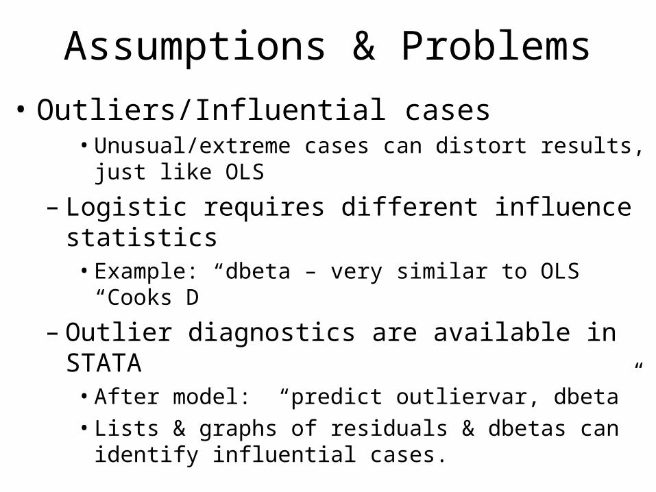
Assumptions & Problems
• Outliers/Influential cases• Unusual/extreme cases can distort results, just like OLS
– Logistic requires different influence statistics• Example: dbeta – very similar to OLS “Cooks D”
– Outlier diagnostics are available in STATA• After model: “predict outliervar, dbeta”• Lists & graphs of residuals & dbetas can identify
influential cases.
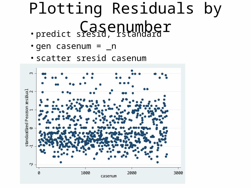
Plotting Residuals by Casenumber• predict sresid, rstandard• gen casenum = _n• scatter sresid casenum
-2-1
01
23
stan
dard
ize
d P
ears
on r
esi
dua
l
0 1000 2000 3000casenum
Assumptions & Problems
• Insufficient variance: You need cases for both values of the dependent variable
• Extremely rare (or common) events can be a problem• Suppose N=1000, but only 3 are coded Y=1• Estimates won’t be great
• Also: Maximum likelihood estimates cannot be computed if any independent variable perfectly predicts the outcome (Y=1)
• Ex: Suppose sociology classes drives all students to drink coffee... So there is no variation…
– In that case, you cannot include a dummy variable for taking sociology classes in the model.

Assumptions & Problems
• Model specification / Omitted variable bias• Just like any regression model, it is critical to include
appropriate variables in the model• Omission of important factors or ‘controls’ will lead to
misleading results.
Probit
• Probit models are an alternative to logistic regression
• Involves a different non-linear transformation• Generally yields results very similar to logit models
– Coefficients are rescaled by factor of (approx) 1.6
– For ‘garden variety’ analyses, there is little reason to prefer either logit or probit
• But, probit has advantages in some circumstances– Ex: Multinomial models that violate the IIA assumption (to be
discussed later).

Example: Unions and Political Participation
• Handout
Example: Coup d’etat
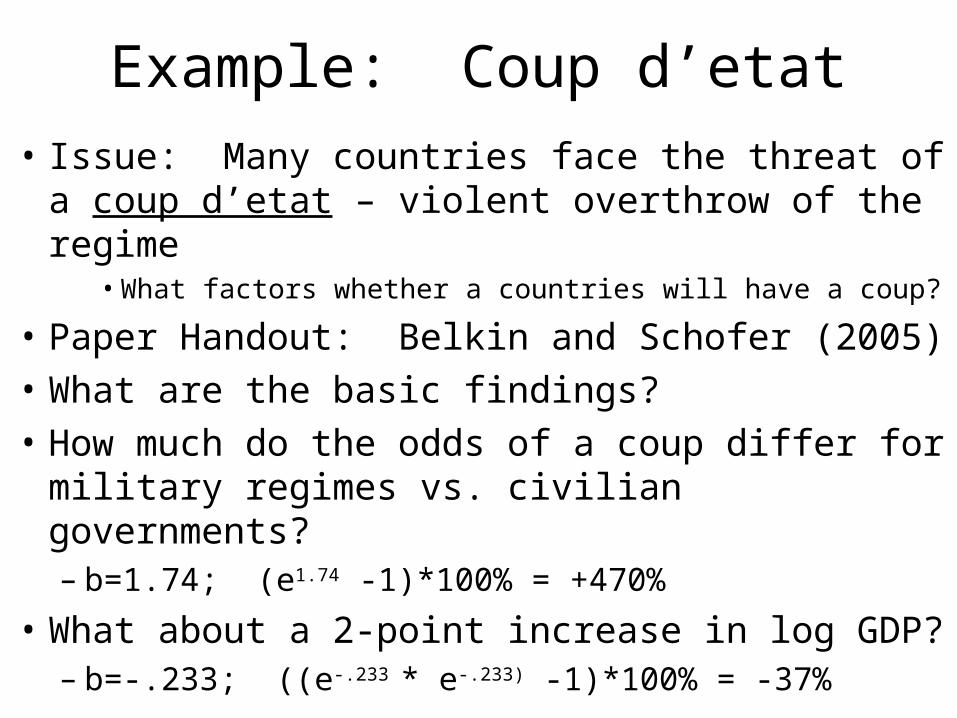
• Issue: Many countries face the threat of a coup d’etat – violent overthrow of the regime
• What factors whether a countries will have a coup?
• Paper Handout: Belkin and Schofer (2005)
• What are the basic findings?
• How much do the odds of a coup differ for military regimes vs. civilian governments?– b=1.74; (e1.74 -1)*100% = +470%
• What about a 2-point increase in log GDP?– b=-.233; ((e-.233 * e-.233) -1)*100% = -37%


