
EVALUATION OF FLUID DYNAMIC EFFECT ON THIN FILM GROWTH IN A
HORIZONTAL TYPE MESO-SCALE CHEMICAL VAPOR DEPOSITION REACTOR
USING COMPUTATIONAL FLUID DYNAMICS
SAHAR TABATABAEI SADEGHI
TONYA KLEIN, COMMITTEE CHAIR
JOHN BAKER
YUPING BAO
ERIC CARLSON
A THESIS
Submitted in partial fulfillment of the requirements
for the degree of Master of Science
in the Department of Chemical and Biological Engineering
in the Graduate School of
The University of Alabama
TUSCALOOSA, ALABAMA
2013

Copyright Sahar Tabatabaei Sadeghi 2013
ALL RIGHTS RESERVED
ii
ABSTRACT
To design and analyze chemical vapor deposition (CVD) reactors, computer models
are regularly utilized. The foremost aim of this thesis research is to understand how thin film
uniformity can be controlled in a CVD reactor. A complete understanding of chemical
reactions that take place both in gas phase and at the deposition surface is required to predict
thin film properties such as growth rate and composition precisely, however, deposition rates
and surface topography can be determined by the arrival flux of reactants in a mass-transfer
limited regime. In order to understand experimental thickness and roughness uniformity, a
predictive model has been developed to study the fluid dynamic effect on thin film growth in
a horizontal type reactor using velocity, temperature, pressure and viscosity as tunable
parameters upon which velocity profiles within a CVD reactor have been evaluated using
computational fluid dynamic (CFD) calculations. Through this predictive model, it is shown
that fluid velocity is the major variable contributing to transverse roll cell formation
compared to temperature and pressure gradients present during thin film deposition in a
meso-scale CVD reactor. These results provide a physical insight regarding improved
reactor operation conditions that influence uniformity.

iii
DEDICATION
This thesis is dedicated to everyone who helped me and guided me through the trials
and tribulations of creating this manuscript. In particular, my parents, my husband and my
advisor who stood by me throughout the time taken to complete this work.

iv
LIST OF ABBREVIATIONS AND SYMBOLS
A Cross sectional area
AFM Atomic Force Microscopy
Ar Argon
ATR Attenuated Total Reflectance
BioMems Bio Micro-Electro-Mechanical System
c Speed of sound
Cp Specific heat
CFD Computational Fluid Dynamic
CVD Chemical Vapor Deposition
d Characteristic length
DPM Discrete Phase Model
Dh Hydraulic diameter
F External body force
FEA Finite Element Analysis
Finfet Fin-Shaped Field Effect Transistor
g Gravitational constant
Gr Grashof number
Convection heat transfer coefficient
H-Si Hydrogen terminated Silicon
HTB Hafnium tert-Butoxide
h

v
HfO2 Hafnium Oxide
Dielectric constant
k Conductivity heat transfer coefficient
kB Boltzmann constant
Kn Knudsen number
L Reactor length in flow direction
Ma Mach number
MOSFET Metal Oxide Semiconductor Field Effect Transistor
P Pressure
Pa Pascal
Pr Prandtl number
Ra Raleigh number
Re Reynolds number
Rf Mems Radiofrequency Micro-Electro-Mechanical System
ss Stainless steel
SiO2 Silicon Oxide
ST Setting temperature
T Temperature
Ambient temperature
Surface temperature
T (subscript) Transpose of the tensor
MKS Meter-Kilogram-Second
N2 Nitrogen
V Velocity
T¥
Tsur

vi
VOF Volume of Fluid
Mean velocity
Density
Del operator
Coefficient of thermal expansion
Dynamic viscosity
Molecular diameter
π Pi
Thermal conductivity
Hydrodynamic entry length
Velocity vector
Molar flux
I Unit tensor
Energy for reaction
Stoichiometric coefficient
Stress tensor
k

vii
ACKNOWLEDGMENTS
I am pleased to have this opportunity to thank Dr. Tonya Klein, my advisor and the
chairman of the thesis committee, for sharing her research expertise and wisdom in addition
to providing motivation for the completion of this work. We would also like to thank all of
my committee members, Dr. John Baker, Dr. Eric Carlson and Dr. Yuping Bao for their
invaluable input and support of both this thesis and my academic progress. Also, I would like
to thank Hamidreza Najafi and Leila Talebi for their efforts and technical supports.
This research would not have been possible without the support of my family who
never stopped encouraging me to persist.

viii
CONTENTS
ABSTRACT .............................................................................................................................. ii
DEDICATION ......................................................................................................................... iii
LIST OF ABBREVIATIONS AND SYMBOLS .................................................................... iv
ACKNOWLEDGMENTS ...................................................................................................... vii
CHAPTER 1 - INTRODUCTION ............................................................................................. 1
1.1 Motivation ............................................................................................................................ 1
1.2 Thesis Layout ....................................................................................................................... 2
CHAPTER 2 - LITERATURE REVIEW .................................................................................. 4
2.1 Chemical Vapor Deposition ................................................................................................. 4
2.2 Micro-Reactors .................................................................................................................... 5
2.3 Buoyancy Driven Roll Type Flow ....................................................................................... 8
2.4 Computational Fluid Dynamic ........................................................................................... 11
2.5 ATR-FTIR Flow in A Horizontal Meso-Scale Reactor ..................................................... 13
2.5.1 Model Study of Meso-Scale Reactor .......................................................................... 14
2.5.2 Study of Thermal Profile in the Meso-Scale Reactor ................................................. 16
2.5.3 Experimental Film Thickness and Roughness Measurement ..................................... 17
CHAPTER 3 - MODELING AND RESULTS ........................................................................ 22
3.1 Introduction ........................................................................................................................ 22

ix
3.2 The Model of Fluid Behavior ............................................................................................ 24
3.2.1 Velocity Effects on the Fluid Behavior ...................................................................... 24
3.2.2 Pressure Effects on the Fluid Behavior ....................................................................... 34
3.2.3 Viscosity Effect on the Fluid Behavior ....................................................................... 41
3.2.4 Temperature Effects on the Fluid Behavior ................................................................ 46
3.2.5 Discussion ................................................................................................................... 56
CHAPTER 4 - CONCLUSION AND FUTURE WORK ........................................................ 58
REFRENCES ........................................................................................................................... 58
APPENDIX A .......................................................................................................................... 63
APPENDIX B .......................................................................................................................... 76

x
LIST OF TABLES
Table 1. List of dimensionless numbers ................................................................................. 12
Table 2. Dimensionless number values; Hydrodynamic entry length at
different velocities .................................................................................................................. 28
Table 3. Observation of roll type flow at μ of 1.663E-5 Pa∙s and different velocities ........... 32
Table 4. Reynolds number at a velocity of 2.3 m/s and different viscosities ......................... 41
xi
LIST OF FIGURES
Figure 1. Transverse velocity vectors (at three axial positions) by ANSYS fluent at
velocity of 58mm/s for: (a) adiabatic side walls, (b) cooled sidewalls [34] (reproduced by
permission) .............................................................................................................................. 10
Figure 2. System set up [47] ................................................................................................... 15
Figure 3. HfO2 thickness on: (a) native oxide (SiO2) with different ST and a bubbler
temperature of 65oC; (b) silicon (Si) with various bubbler temperatures and a ST of
250oC (lines are only to guide the eye and do not represent a statistical
fit to the data) [47] .................................................................................................................. 20
Figure 4. (a) 3-D AFM image of a H-Si (100) surface after adsorption of HTB for 1 hour
using a bubbler temperature of 65oC and a substrate temperature of 250
oC showing an
undulating topography towards the exit of the reactor cell, L = 3cm (b) quantitative AFM
analysis of the sample shown in (a) showing a periodicity of 10 nm [47] ............................. 21
Figure 5. Three cross-sections for velocity analysis ............................................................... 26
Figure 6. Transverse velocity vectors (at three axial positions) for a velocity
of 0.001 m/s ............................................................................................................................ 27
Figure 7. Transverse velocity vectors (at three axial positions) by ANSYS fluent at
velocity: (a) 0.07m/s, (b) 0.34 m/s, (c) 0.86 m/s ..................................................................... 30
Figure 8. Transverse velocity vectors by ANSYS Fluent at V = 2.3 m/s ............................... 31
Figure 9. Velocity vectors at: (a) 5.7m/s, (b) 10.4 m/s, (c) 14.7 m/s ...................................... 34
Figure 10. The flow behavior at the velocity of 2.3 m/s and d pressures of: (a) 0.1 Pa, (b)
40 Pa, (c) 100 Pa ..................................................................................................................... 36
Figure 11. Flow behavior at velocity of 6.8 m/s and pressure of (a) 0.1 Pa, (b) 40 Pa, (c)
100 Pa...................................................................................................................................... 38
Figure 12. Transverse velocity vectors of the flow at the velocity of 11.6 m/s and pressure
of: (a) 0.1Pa, (b) 40 Pa, (c) 100 Pa.......................................................................................... 40
Figure 13. Transverse velocity vectors at the velocity of 2.3 m/s and the viscosity of: (a)
1.663E-5 Pa.s, (b) 1.663E-4 Pa.s ............................................................................................ 42

xii
Figure 15. The numerical modeling at the velocity of 11.6 m/s and the viscosity of: (a)
1.663E-5 Pa∙s, (b) 1.663E-4 Pa∙s ............................................................................................ 45
Figure 16. Velocity vectors using an inlet value of 2.3 m/s and a top plate temperature of:
(a) 250˚C, (b) 347˚C, (c) 547˚C .............................................................................................. 47
Figure 17. Velocity vectors for an inlet velocity 6.8 m/s and a top plate temperature of:
(a) 250˚C, (b) 347˚C, (c) 547˚C .............................................................................................. 49
Figure 18. Transverse velocities at three axial locations for an inlet velocity of 6.8 m/s
and top plate temperatures of: (a) 250˚C, (b) 347˚C, (c) 547˚C ............................................. 50
Figure 19. Transverse velocities at three axial locations for velocity of 2.3 m/s and the
temperature of: (a) 250˚C, (b) 347˚C, (c) 547˚C .................................................................... 52
Figure 20. Transverse velocities at three axial locations for velocity of 6.8 m/s and
bottom plate temperatures of: (a) 250˚C, (b) 347˚C, (c) 547˚C .............................................. 54
Figure 21. Transverse velocities at three axial locations for an inlet velocity of 11.6 m/s
and bottom plate temperatures of: (a) 250˚C, (b) 347˚C, (c) 547˚C ....................................... 56
Figure 22. AFM images of film topography on native SiO2 substrates for three positions
along the flow direction in a meso-scale CVD reactor. Top image is at the exit side
(L=3cm). ................................................................................................................................. 57

1
CHAPTER 1
INTRODUCTION
1.1 Motivation
The use of thin film growth techniques such as Chemical Vapor Deposition (CVD)
allows production of high-quality epitaxial thin films [1-4]. To grow polycrystalline Si,
dielectric materials and passiving films utilized in manufacturing of Si integrated circuit, the
horizontal CVD reactor has long been used as the chief product tool among other types of
CVD reactors such as stagnation flow reactors and low-pressure multi-wafer barrel-type
reactors [5]. Over the last several decades, CVD has been the chief traditional thin film
deposition technique in industry. Composition, adhesion, surface morphology and purity are
some controllable properties of thin films that are produced through thin film production
processes. Since HfO2 has a reasonably, high κ value, and a high thermodynamic stability on
Si, it is used for various applications [6]. As a case in point, it is used as a gate insulator in
metal-oxide semiconductor field-effect transistors (MOSFETs), and in FinFET double-gate
transistors [7]. In addition, it has many applications in catalytic oxidative dehydrogenation as
a porous support [8] and in radio frequency micro electromechanical system (RF MEMs) as a
shunt switch flexible capacitor [9]. Moreover, due to having high refractive index, HfO2 is
applied as an optical coating for laser mirrors [10]. Achieving uniformity in thin films is an
important part of the optimization of deposition processes and reactor design [11-13]. Hence,
selection of CVD process parameters is very critical for achieving uniformity on substrates.
The need for precise definition on a one-micron scale and over high aspect ratio geometries
2
makes the importance even greater. One measure of thin films uniformity is of thickness and
composition. This is specifically important for the micro-electronic industry in which fine
resolution of devices is critical.
Deposition uniformity is dependent upon two factors, reactant spatial uniformity and
depletion of resulting by-products via deposition. The variation in the concentration of
precursor from the inlet to the outlet of the reactor considerably depends on the length of
flow path and loading of substrate. For the immobile wafer at the leading edge of the wafer,
the concentration of flow and deposition rate is the highest, and the boundary layer is the
thinnest. If the reactants are consumed when the carrier gas reaches the exit port, then the
reactant utilization has the highest efficiency. However, this causes the deposition not to take
place near the exit and on the wafer surface and hence, a starved reaction condition happens.
Since an increase in temperature leads to an increase in substrate diffusivity, the effect of
reactant depletion and an increase in boundary layer thickness can be compensated by an
increase in flow velocity and temperature [14]. Since depletion of reactants and stationary
eddies has long been a concern in cold wall reactors, computational fluid dynamics has been
used to evaluate the dynamics of the fluid on the growth film.
1.2 Thesis Layout
The main step in this modeling effort is developing a CFD model. Then, the model
has been applied to study the effect of setting parameters such as velocity, temperature and
pressure on fluid behavior such as the formation of eddies and rolls in the flow. Precise
prediction is of great importance for the optimization of setting parameters to achieve the
best uniformity. The focus of this thesis is to complete this step. In previous research,
hafnium tert butoxide (HTB) has been used as a precursor to deposit HfO2. In this work,

3
rather than HTB, N2 has been used as an inert gas to simplify the model and the reactive flux
of precursor to the surface is not incorporated into this model.
4
CHAPTER 2
LITERATURE REVIEW
2.1 Chemical Vapor Deposition
CVD is a process to grow thin films with preferred properties. In this technique,
source vapors contact a heated substrate and deposit via a chemical reaction on the surface to
generate the needed material [15]. In the other words, premixed gases chemically react and
on a heated substrate to from a solid crystalline or amorphous layer. The process has four
main steps: First, reactants are transported to the susceptor. Second, the chemical reactions
take place. Third, new species are generated and finally the reaction products are desorbed
diffused back to the main stream [16]. Based on various applications, different materials,
various CVD process types and various shape and design of CVD reactors, the substrate
temperature is adjusted [17,18]. This technique has many applications in various fields such
as the production of computer hardware comprising transistors, UV detectors, integrated
circuits and blue light emitting. Likewise, it is applicable in electrostatic loudspeakers, a very
important element in the fabrication of electronic components, semi-conductors, coating of
machining tools, optical and corrosion applications, and in nuclear applications, magnetic
recoding media, and solar cells [19,20]. Real time feedback control of the CVD process is
very important since there is a high demand for precision of preferred properties of the film
layer such as thickness and composition [21-24]. There are different chemical reactions
taking place in CVD. These reactions include hydrolysis, disproportionation, carburization,
thermal decomposition (pyrolysis), reduction, nitridization and oxidation [25]. To control
5
CVD processes, there are various factors to be considered including mass transport, kinetics,
thermodynamics, the chemistry of the reaction, chemical activity, temperature, and pressure.
Most CVD reactors are divided in two general types based on their shape and orientation of
process gas flows: vertical and horizontal reactors. In the first class, the downward incoming
flow is perpendicular to the heated susceptor but in the second class, the fluid flow is parallel
to the angle of the susceptor.
Generally CVD processes are divided in two categories: thermal or conventional
CVD (original process) and plasma, laser, and photo CVD. Thermal CVD is classified by
two kinds of reactors known as the hot wall reactor and the cold wall (adiabatic wall) reactor.
This organization is based on the need for high temperature. High frequency induction,
radiant heating, resistance heating and hot plate heating can produce the needed temperature.
The other category is plasma, laser and photo CVD. This division is based on the approach of
applying energy necessary for the CVD reaction to happen.
CVD has some advantages and disadvantages. As a case in point, it can provide
conformal, homogeneous and dense isotropic films even though channels have high aspect
ratio. While sometimes, it is very hard for CVD to control film thickness. Therefore, it is
possible that thin films become rough and even discontinuous and broken because of growth
nucleation. By growing thin films on various substrates, optoelectronic devices and advanced
electronic such as radar systems and computer chips are developed.
2.2 Micro-Reactors
In general, micro-technology is expressed as technology having microstructures in the
range of one millimeter or less. Typically, micro-reactors, micro-tubes, micro-pumps are

6
categorized in the microstructures class. There are various limitations for such micro scale
devices such as fabrication, testing, visualization and assembling [26].
A micro-reactor is a well-suited device for kilogram-scale processes. Also, it is used
for specialty chemical productions. For these reactors, the range of internal diameter and the
order of specific surface area respectively is 10- -50,000 m2. Because of
these range limits, the transfer of the heat is high, which can be useful for highly exothermic
reactions [27,28].
For organometallic reactants, micro-reactors facilitate the fast exothermic and
endothermic reactions. Another aspect of these kinds of reactors is that the residence time
distribution is minimized [27]. In these reactors, the ability to control residence time is good,
and the transfer of heat is fast, however, mixing can be problematic, since it is mostly by
diffusion with very limited convective mixing [29]. On the other hand, according to a study
by Dessimoz et.al., micro structured reactors are appropriate devices for separating and
mixing varieties of phases (liquid-liquid, gas-liquid and gas-gas phases) [27]. Mixing
methods are classified into three categories including contact-type for accurately monitoring
the interface, segmented flow and micro mixer [30].
Also, micro-reactors are well suited for conducting dangerous reactions that are
hazardous when performed at a large scale. These reactions can be classified using various
categories such as high temperature reactions, exothermic reactions, and reactions involving
unstable intermediates and dangerous reagents [31].
Generally, the elementary or intrinsic scale is the so called macro-scale in which
performances are presumed or given as input. In this scale, parameters such as flow rate,
pressure and temperature are monitored to attain the best product conversion and minimum
consumption of power and emissions of pollutant. At the micro-scale, these performance
7
objectives are also measurable and adjustable. As a case in point, we can mention the single
particle as a micro-scale for a fluidized bed reactor.
Between these scales, there is the meso-scale in which time and space are
considerable and they are known by heterogeneous structures (i.e. clusters and bubbles).
Hence, to grasp total range of scales, the meso-scale is the link between micro and macro-
scale. Meso-scale has characterizations between micro- and macro-scale with variety of
heterogeneous structures to which micro-scale structures may respond nonlinearly. The
behavior of individual particles in meso-scale is not similar to isolated particles. Thus one
cannot simply average the single particle behaviors to study the meso-scale. This is the
reason why a reactor must be scale-up, and therefore, the understanding of meso-scale
structures in depth is essential [32]. In meso-scale reactors, due to large diffusion times and
high heat transfer to the channel wall, bulk chemicals are produced. In spite of having high
exothermic reactions, operation of meso-scale reactors is almost isothermal. This results to
excellent selectivity.
Generally, in various fields such as biomedical and aerospace, the need for meso-
devices ranging from100 μm-10 mm is high and micro devices ranging from 0.1-100 μm and
with high aspect ratios are also needed [33]. It has been stated that meso-(100 μm-10 mm) or
micro-(0.1-100 μm) devices which have high aspect ratios is in high demand in the
aerospace, biomedical, optical, and micro-electronics packaging industries [25,34]. There is a
high demand for fast, direct, and mass fabrication of meso or micro efficient products from
polymers, composites, and ceramics. In contrast, a growing need to produce semiconductor
products or materials for biomedical applications, the technology for mass fabrication of
meso or micro parts are not still developed [35]. Based on research by Kuski, et.al, micro-
reactors are known as differential reactors or small-scale reactors that were used as an initial
8
step of scale-up before. But, nowadays, they are used as the last step of process development
[36]. In micro-reactors, the heat transfer rate between reactants and reactor surface is
considerable. Therefore, temperature can be controlled accurately and fast. Also, micro-
reactors are one of the appropriate tools for generating toxic or explosive chemicals. Another
characteristic of micro-reactors is that they are used for two-phase reactions (gas-liquid and
liquid-liquid). One of the key factors of micro-reactor is for the preparation of catalysts.
2.3 Buoyancy Driven Roll Type Flow
Buoyancy driven flow has an important effect on the performance of a CVD reactor
utilized for thin solid film deposition [37-41]. There are many groups studying visualization
and numerical computations of mixed convection flows, their importance in transporting the
reactants to the substrate [19], [42,43] and their influence for controlling the process.
In some studies, it has been shown that buoyancy-induced flow can trigger
recirculating eddies and move reactants away from the substrate. These buoyancy driven
flows not only reduce growth rate but also the uniformity of a film. In general, less than a
percent change in thickness of the film is unsatisfactory for high quality applications. To
improve the performance of CVD reactors, the configuration of the reactors, and setting
parameters can be modified in a way to achieve required flow fields and improved movement
of reactants to the substrate. This causes an increase in growth rate in a way to maintain a
uniform thickness.
When buoyancy forces are associated with heat or mass transfer, they dominate
diffusion and viscosity forces and this causes instability situations in a fluid layer. Therefore,
secondary motion (longitudinal and transversal vortex rolls) will occur and provide mixed
convection. Chemical vapor deposition, heat exchanger, electroplating are examples of
9
processing systems prone to form roll-type instability. Non-linear, developing temperature or
concentration profiles in these processes are a problem for predicting a situation of
buoyancy-driven motion [42].
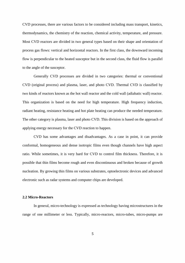
Numerical simulation of buoyancy driven flow in a horizontal reactor was evaluated
to showing the convection driven roll pattern development, where two kinds of models were
used. One of them was based on adiabatic sidewalls and the other one was based on cooled
sidewalls with the same condition. Figure 1 shows that the rotation of the convection rolls for
both cases are reverse.
In the first situation, at the first, the gas expands due to its contact with the hot
susceptor then rolls are shaped in the corners and close to the end of the reactor. This roll
type flow appeared due to presence of less heated fluid in the mid-plane, which is created due
to a density gradient between the faster moving fluid and the slower moving streams at the
corners. By developing the flow, there is no density gradient. Therefore, the rolls disappear.
(a)

10
(b)
Figure 1. Transverse velocity vectors (at three axial positions) by ANSYS fluent at velocity
of 58mm/s for: (a) adiabatic side walls, (b) cooled sidewalls [34] (reproduced by permission)
In the second situation, initially the gas enlarges fast because contact with the hot
susceptor. According to Jenson’s paper, the spatial uniformity of growth rate is affected by
buoyancy driven secondary flow and the structure of the flow is dependent on the thermal
boundary condition, the kind of carrier gas and the aspect ratio of the cross-section.
Furthermore, as the aspect ratio decreases, the effect of buoyancy driven rolls is reduced
[34].
Based on S. Ostrach and Wilbert J’s study, there are two kinds of flow produced via
buoyancy. These flows are called convectional convection and unstable convection. In the
first case, a density gradient is perpendicular to the gravity vector and this causes ensuing

11
flow. In the second case, the density gradient is opposed to the gravity vector but parallel to
it and this provides unstable equilibrium in the fluid [35].
The characteristics of CVD processes are affected by mass transfer and mixed
convective heat. This subject has been investigated for a long time in horizontal CVD
reactors. Due to the mixed convective heat in these reactors heated via a lower wall, the
longitudinal recirculation and return flow probably occurs. The uniformity and growth rate of
the thin films are affected by return flow [45]. In 1997, Makhviladze and Martjushenko
studied various features of the transverse recirculation formation in horizontal CVD reactors
[46]. They determined return flow formation could be independent on the width of the
reactor and the amount of the cooling of the sidewalls (cooled or adiabatic walls). The cooled
walls delay the formation of the vortex compared to adiabatic walls. This is due to the
longitudinal rolls formation taking place at all non-zero Grashof number (Gr). By increasing
the Gr, the longitudinal rolls increase. Also they investigated that recirculation is more likely
happen close to the sidewalls than at the reactor center and at the onset of the formation of
the vortex when ratio of Gr to Re (Gr/Re) is still very low, the probability of the occurrence
of recirculation in the bulk gas is very low. In addition, the smaller the width of the reactor,
the more the return flow formation will be suppressed [46].
2.4 Computational Fluid Dynamic
The term, Computational Fluid Dynamic (CFD), is mainly related to the motion of
fluids and is the study of the behavior of fluid flow on heat transfer and chemical reactions
using numerical simulation. Furthermore, in CFD, the physical features of the fluid motion
can be explained via fundamental mathematical equations in partial differential form termed
the governing equations. Also, using CFD, flow conditions, which do not have capability to

12
be reproduced in experimental tests, are simulated. In the end, CFD visualizes and gives
broad information as compared with experimental fluid dynamics. In order to being effective
for developing fluid-system designs, CFD could provide insight into designs being evaluated
over a range of dimensionless numbers containing Mach number, Rayleigh number, and
orientation of the flow. Table.1 shows few dimensionless numbers and their corresponding
equations.
Table1. The list of dimensionless numbers
Dimensionless number Definition
Reynolds number
Grashof number
Rayleigh number
Mach number
Prandtl number
Knudsen number
Flows could be either compressible or incompressible and many of them have
nonlinear characteristics and do not have an analytical solution. Hence, a search is motivated
for numerical solutions containing partial differential equations. CFD has many applications
in many different fields. As a case in point, it is applicable to investigate fluidization

13
behavior of solid–liquid flow to develop the efficiency of limestone application in a conical
reactor [21]. Also, it is a process that is used to enhance fluidized bed combustor and
gasifiers [22]. Likewise, a tabular aerodynamic, which is produced with validation against
wind tunnel experiments is modeled using CFD predictions [23]. In addition, a multi-scale
model is developed throughout CFD to explain silicon particle growth using CVD in a
fluidized bed reactor. Hydrodynamics using momentum, mass and heat transfer among
various phases are described by CFD [24].
2.5 ATR-FTIR Flow in A Horizontal Meso-Scale Reactor
By having information about the mechanism of film growth, precursors and the
process of mass transport, we can grasp thin film deposition by chemical reaction. Film
morphology is dependent on the deposition process on the surface of the growing film, which
is related to the chemical reactivity of precursors. In addition to chemical properties of the
precursors, the phenomena of mass transport have are important. Thus, controlling the spatial
distribution of precursor compounds is very essential for formation of the film. It has been
shown that the microstructure and composition of the film depend on deposition conditions
under which the film was grown. As we mentioned in preceding chapters, the formation of
thin film by transforming the molecules in gas phase into surface material having a diverse
composition is named chemical vapor deposition. In this process, in order for a solid
deposited material to form, the reaction of chemical components on a substrate takes place.
Physical and chemical processes in CVD are comprised of surface chemistry, gas-phase,
multi-component mass transfer, heat transfer and gas dynamics. According to Patnaik’s
study, the essential factors in the CVD are precursor gas flow rates, pressure, temperature
and the reactor geometry. He determined that the geometry has effect on fluid behavior [33].

14
In the other words, the understanding of fluid dynamics would assist in the design
optimization. In Li et.al study, morphology, kinetics of film growth and composition were
examined to show the influence of reactor geometry on gas fluid behavior [47]. In most
times, CFD was chosen to model the CVD process. In that research, an undulating
topography for thin films (HfO2) on various substrates (borosilicate glass, Si, and native
SiO2,) in a meso-scale reactor was evaluated. Due to difficulty in a CVD reactor, the effect of
the transport of precursor vapor on the kinetic behavior of film growth has been modeled. In
that research, hafnium tert-butoxide (HTB) was used as a precursor to deposit hafnium oxide
(HfO2) in the CVD reactor. HfO2 is a high-k gate dielectric film grown on different substrates
by CVD [47]. The purpose of this effort was to improve a direct gate dielectric deposition
process to accomplish continued device scaling preserved for more than 3 decades
The thickness of the gate dielectric materials is about 2 nm but one of their flaws is
that they do not have the ability to be scaled with recent materials. Due to having particular
properties such as thermal stability, low defect density and being an outstanding insulator,
SiO2 is chosen as a gate dielectric but has some limits. One of the alternative gate dielectric
materials is HfO2, which has a comparatively high resistivity and dielectric constant.
Moreover, at or less than 1000˚C, it is thermally stable with silicon and compatible with n
doped poly-silicon. CVD is a good method to control homogeneity of the film and interface
and it is good technique to deposit a high-k film [48].
2.5.1 Model Study of Meso-Scale Reactor
As we stated, thin films of HfO2 were deposited in a meso-scale reactor. The design
of the reactor is such that it is compatible to an inflow of a vaporized metal organic precursor
and an outflow at vacuum. The schematic of the reactor components include a source

15
bubbler, an Edwards rotary vane pump, two MKS Piani gauges, an Ar bypass line, and a
stainless steel flow reactor with two tubes placed at the inlet and outlet of the reactor. Figure
2 shows schematic of experimental set up.
Figure 2. System set up [47]
In this system, the transmission of HTB under N2 into the bubbler was done. The
bubbler was preheated (45 min) using oil bath at temperatures ranging from 50-75˚C and at a
vapor pressure of 9.3 Pa to 133.3 Pa. Then the precursor was moved to the flow cell. The
purpose of the two Pirani gauges located on both sides of the flow cell was to measure the
pressure difference. Based on the temperature of the reactor and the bubbler, the
experimental pressure was 40 Pa (5332.89 torr) and the base absolute pressure for a gauge
placed on the downstream was 0.13 Pa (17.331 torr). It was shown that when the temperature
of the bubbler and flow rates increased, the pressure drop decreased, and when the crystal
temperature increased, the pressure drop increased.

16
Since the vapor pressure of HTB is high, no carrier gas was utilized. Next to the
bubbler, there was an Ar bypass line that before and after each experiment, its purpose was
for regulating the flow rate and purging the gas line. In the meso-scale reactor, a substrate
was at the bottom plate of the reactor and it had the ability to be changed. The heat of the
reactor came from two copper heating rods. In the other words, these two copper heating rods
generated heat and determined the temperature at the top and bottom plates. The
thermocouple in the top plate controlled the setting temperature up to 250˚C. The Omnic
temperature controller controlled the temperature. After giving a set point temperature, the
power of the heating rod could be adjusted accordingly when there was some fluctuation in
the temperature. So transiently, there could be a temperature reduction on the heating plate.
Hence, the temperature controller did a good job to keep a constant temperature of 250˚C.
When the setting temperature was increased, the temperature gradient between top and
bottom plate (the substrate) increased to around 100˚C.
2.5.2 Study of Thermal Profile in the Meso-Scale Reactor
Achievement of uniform composition and conformal topography is an important goal
in thin film industrial applications. A critical parameter to meet this end is fluid and substrate
temperatures as these are the drivers for adsorption, diffusion, reaction and desorption
kinetics during the process of deposition. In turn, a smaller substrate temperature gradient,
results in better uniformity of the deposited film in both thickness and composition. Since
the substrate is contained in a small, vacuum sealed vessel, with the thermocouple placed at
one spot near the substrate surface, obtaining the temperature profile along deposition surface
in the vapor flow direction was not possible. Consequently, finite element analysis (FEA)

17
was used to calculate the temperature gradient on the surface. Using FEA, heat transfer
conditions were simulated using the reactor geometry and materials design.
In addition to conduction, thermal heat was lost by convection of heat due to the flow
conditions and the distribution of temperature along the substrate. Using the FEA simulation,
the loss of thermal heat was determined. The geometry used was the actual meso-scale
reactor dimensions. The heat source is from two copper rods with a power of 0-100W, for
which the setting determined the substrate temperature. At a steady state condition, and at
the plane exposed to air, a heat transfer equation may be obtained by setting the convection
and conduction rates to equivalent values.
(1)
At , (2)
In spite of the huge volume of the substrate compared to the thin film volume, the
released heat from deposited thin film did not have an effect on the temperature of the
substrate.
2.5.3 Experimental Film Thickness and Roughness Measurement
In this study, the thickness and the roughness of the film at different bubbler (vapor)
temperatures and substrate set-point temperatures (ST) were evaluated. The deposition time
and deposition rate are two important factors that have an impact on film thickness. Based on
the precursor supply rate, which is determined mainly by the temperature of the bubbler (and
less so by the pressure gradient which was not considered here), accumulation and depletion
of the precursor along the substrate surface took place. In addition, substrate temperature
affected the consumption of the precursor, and also diffusion and desorption. Figure 3 (a)
depicts the HfO2 thickness on native silicon oxide (SiO2) for ST 225, 250 and 300˚C and a
-k ×A ×ÑT +h(T¥ -Tsur ) = 0
CT 25 02 T

18
bubbler temperature of 65˚C while (b) shows the effect of bubbler temperature (precursor
flux) at a ST of 250˚C [53]. The figure shows that the precursor can accumulate or become
depleted along the flow axis depending upon the substrate temperature. For a ST of 300˚C
the larger thickness at the entrance and depletion along the axis indicates the precursor has
enough energy at the surface to decompose and react, while at 225˚C the thickness increase
along the flow axis shows a decreased reaction probability requiring more precursor/reaction
site interactions and/or surface diffusion before a precursor molecule reacts. At the
intermediate ST of 250˚C the best uniformity was achieved without an accompanying
compromise in growth rate. Interestingly, optimum conditions were found halfway down the
reactor length, which corresponds to the point of eddy formation as described in later
sections. This implies that a perpendicular component to bulk flow is beneficial for precursor
utilization. Another possibility is that multiple collisions with the substrate are needed before
enough energy was gained for decomposition and reaction to occur. In the second part of the
study, the effect of precursor temperature from the bubbler was evaluated. In addition, a
larger bubbler temperature results in a larger precursor flux.
In Figure 3 (b), the bubbler temperature was varied with values of 40oC, 50
oC, 65
oC,
and 75oC using a ST of 250
oC. At the two lower temperatures a low precursor flux resulted
in a reduced growth rate, however, the uniformity was good. Also, the lower temperature
may have limited the degree of decomposition, requiring surface diffusion and/or multiple
adsorption events before reaction could occur. At the higher temperature of 75˚C, a larger
precursor vapor flux results in an increased thickness and deposition rate, while the increased
thermal energy of the arriving molecules may allow for enhanced surface diffusion and
multiple physisorption, desorption, and re-adsorption events leading to a build-up of
thickness towards the back-end of the reactor cell. Most interesting is the trend seen at the
19
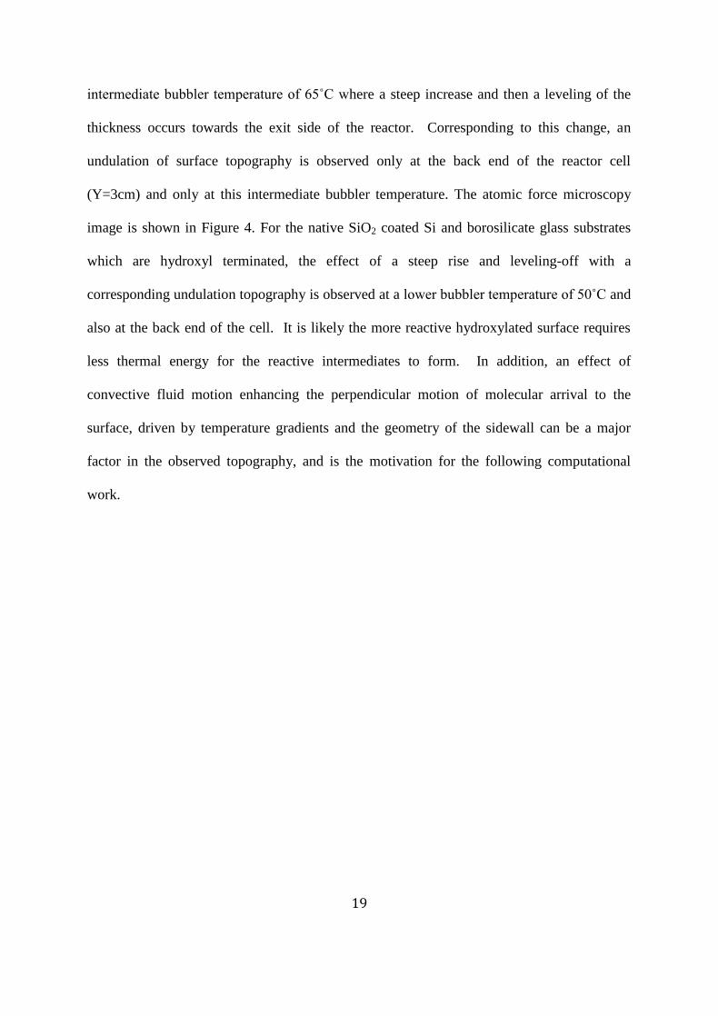
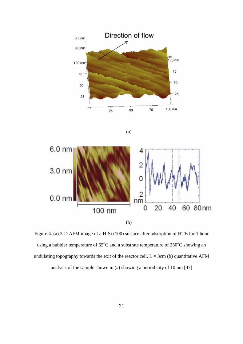
intermediate bubbler temperature of 65˚C where a steep increase and then a leveling of the
thickness occurs towards the exit side of the reactor. Corresponding to this change, an
undulation of surface topography is observed only at the back end of the reactor cell
(Y=3cm) and only at this intermediate bubbler temperature. The atomic force microscopy
image is shown in Figure 4. For the native SiO2 coated Si and borosilicate glass substrates
which are hydroxyl terminated, the effect of a steep rise and leveling-off with a
corresponding undulation topography is observed at a lower bubbler temperature of 50˚C and
also at the back end of the cell. It is likely the more reactive hydroxylated surface requires
less thermal energy for the reactive intermediates to form. In addition, an effect of
convective fluid motion enhancing the perpendicular motion of molecular arrival to the
surface, driven by temperature gradients and the geometry of the sidewall can be a major
factor in the observed topography, and is the motivation for the following computational
work.

20
(a)
(b)
Figure 3. HfO2 thickness on: (a) native oxide (SiO2) with different ST and a bubbler
temperature of 65oC; (b) silicon (Si) with various bubbler temperatures and a ST of 250
oC
(lines are only to guide the eye and do not represent a statistical fit to the data) [47]
21
(a)
(b)
Figure 4. (a) 3-D AFM image of a H-Si (100) surface after adsorption of HTB for 1 hour
using a bubbler temperature of 65oC and a substrate temperature of 250
oC showing an
undulating topography towards the exit of the reactor cell, L = 3cm (b) quantitative AFM
analysis of the sample shown in (a) showing a periodicity of 10 nm [47]

22
CHAPTER 3
MODELING AND RESULTS
3.1 Introduction
In the previous section describing the measured experimental results of thickness and
topography, the effect of gas flow dynamics within the vapor space of the reactor is
suspected to become determinant under certain intermediate precursor flux and substrate
temperature conditions. Faced with this possibility, herein is described a set of computational
fluid dynamic (CFD) simulations undertaken to elucidate the vapor flow effect during thin
film deposition at the meso-scale. For this model, due to a temperature gradient between the
top and the bottom plate and the geometry of the flow cross-section, a roll-type flow
perpendicular to the deposition plane took place that was related to the Ra number. This
phenomenon was identified as the Benard thermal instability [15]. In the present work, a
CFD model was developed to determine the degree to which pressures, viscosity,
temperature gradients and velocities affected the type of roll cells predicted (transverse) and
with special attention to values of the Rayleigh and Grashof dimensionless parameters. Also
considered, was the entrance length need for fully developed flow. For this first
comprehensive sensitivity analysis of deposition parameters, the simulated gas chosen was
pure N2, and deposition flux was not considered.
This simulation and modeling was done using ANSYS Fluent 13 through Linux
systems on Mammoth (http://unix.eng.ua.edu/). The ANSYS Fluent is computational fluid
dynamics software in which fluid flow and other physical phenomena are modeled. This
23
software is a multifunctional one. In the other words, through this software, fluid flow, which
can comprise broad range of flows such as compressible flow, inviscid flow, periodic flow
and so forth under steady state or transient conditions can be computed. Furthermore, the
governing equations and physical models are modeled via ANSYS Fluent. The governing
equations are set of Navier-stokes (N-S) equations for viscose, heat conducting fluid
including momentum conservation, continuity and energy balance. Via implicit or explicit
methods in the infinite volume approach, the velocities and pressure can be solved by
iteration. For steady state incompressible flow, continuity, momentum conservation and
energy balance can be written respectively as follow [47,49]:
Continuity (3)
) Conservation of momentum (4)
where: )
[ -
)] Energy balance (5)
To model complicated geometries, mathematical models for transport phenomena are
combined with the capability. In industrial activities, there are different characteristics to
allow modeling of the fluid flow. These features contain heat transfer, lumped parameter,
moving reference frame models and so on. Multiphase flow model, time accurate sliding
mesh and free surface set are a practical set of models, which are utilized for analysis of
various multiple-phase flow flows. Hence, ANSYS Fluent runs different models that are
known as DPM, VOF and Eulerian models.
Robust and Accurate Turbulence models are named as fundamental elements of the

24
suite of models. These models could be applied in a wide range including buoyancy and
compressibility. Other than these models, the ANSYS Fluent can model different
mechanisms of heat transfer, containing mixed and forced convection, combustion
phenomena comprising scattering of eddies and function of probability density models.
Moreover, the creations of pollutants and surface reaction models have been developed [49].
3.2 The Model of Fluid Behavior
3.2.1 Velocity Effects on the Fluid Behavior
Of the parameters explored, velocity has the largest impact on eddy formation and
roll type flow, which is assumed to influence observed film properties such as thickness and
topography. In this section, we modeled the stream velocity of an inert gas, N2, under a
steady state flow condition. To simplify the model, some assumptions have been made. First,
a steady state condition was assumed in the determination of the temperature distribution.
Second, at temperatures less than 250oC, radiation heat transfer can be assumed negligible.
Third, between the top and bottom plates, thermal contact the resistance is assumed
insignificant. Fourth, the transfer speed of reaction heat through the thin film was fast, owing
to the small thickness scale of less than 1 micron. Fifth, a flux of material to the surface due
to deposition was considered negligible. Last but not least, due to the density of the fluid and
the dimension of the reactor, we assumed a nonslip condition at the reactor walls consistent
with viscous, laminar flow. The nonslip assumption rests upon the determination of a key
dimensionless parameter, the Knudsen number (Kn).
The Kn number is a ratio of the mean free path (λ) and the characteristic length of the
reactor geometry (d). The mean free path is the mean distance that a particle travels in a gas
before encountering a collision with a gas molecule and is dependent on molecular density,
25
which is the pressure. Using the Kn number, fluid flow can be classified into three regimes.
If the Kn number is bigger than one (Kn >1), the flow is known as a molecular flow for
which the number of collisions with the reactor wall is more than the number of collisions
between the molecules themselves, and the no slip boundary condition assumption fails. If
the Kn number is between 0.01 and 1 (0.01< Kn<1), the flow is in transition, while if the Kn
number is less than 0.01 (Kn<0.01) the flow is considered viscous where a no slip condition
is virtually guaranteed. For an ideal gas the mean free path is formulated as follows: λ =
kBT⁄(√2 πσ2Ρ) in which kB is the Boltzmann constant, T is the thermodynamic temperature, σ
is the molecular diameter of the particle, π is 3.14 and P is the total pressure [50]. In this
case, d, the characteristic length, is the height between the top and bottom plate, which is 4
mm, and the mean free path (λ) is 2.9×10⁻⁴
m for a pressure of 40 Pa. Hence the Kn is 0.07
and the flow is within the transition regime, but close to viscous. If the hydraulic diameter,
Dh, is used as the characteristic length (Dh is four times the cross-sectional area divided by
the perimeter of the plane perpendicular to the flow direction and is 10.45 mm), the Kn is
0.027, even closer to a viscous flow assumption.
Fluid behavior was evaluated at different arbitrary velocities ranging from .001 m/s to
14.7 m/s in the flow cell. Experimentally, it was not possible to accurately determine the
evaporation rate of the precursor from the bubbler. The top plate and the bottom plate
temperatures were 250oC and 150
oC respectively. To observe the fluid behavior in the flow
cell, three cross-sectional planes perpendicular to the flow axis of the horizontal reactor were
selected at positions near the inlet, center and outlet at values for L= 0.01, 0.02, and 0.04 m,
where the total reactor length is 5 cm. A diagram of the modeled reactor showing the three
plane positions is shown in Figure 5.

26
Figure 5. Three cross-sections for velocity analysis
In Figure 6, the velocity vectors for an inlet velocity of 0.001 m/s at the three
positions down the length of the reactor is shown. This figure gives insight into the velocity
variation in the reactor. The velocity arrows have a length proportional to the velocity
magnitude relative to the flow direction along the x coordinate. The colored scale on the left
side displays velocity magnitude contour plots representing the square root of the sum of the
squared velocities in x, y and z directions.
It is observed that the flow behavior in the horizontal CVD reactor is correlated to the
Reynolds, Re, and Grashof, Gr, dimensionless parameters. It was seen that when the inlet
velocity was set to the lowest value of 0.001 m/s, no transverse rolls were observed at the
inlet, outlet or middle of the reactor. At this velocity, the measured Reynolds number was a
small value of 0.055 indicating that viscous forces override inertial forces. Also, the ratio
Gr/Re2
was 5420,000. When Gr/Re2
is much bigger than one, natural convection is significant
and dominant over forced convection. When Gr/Re2
is much less than one, natural convection
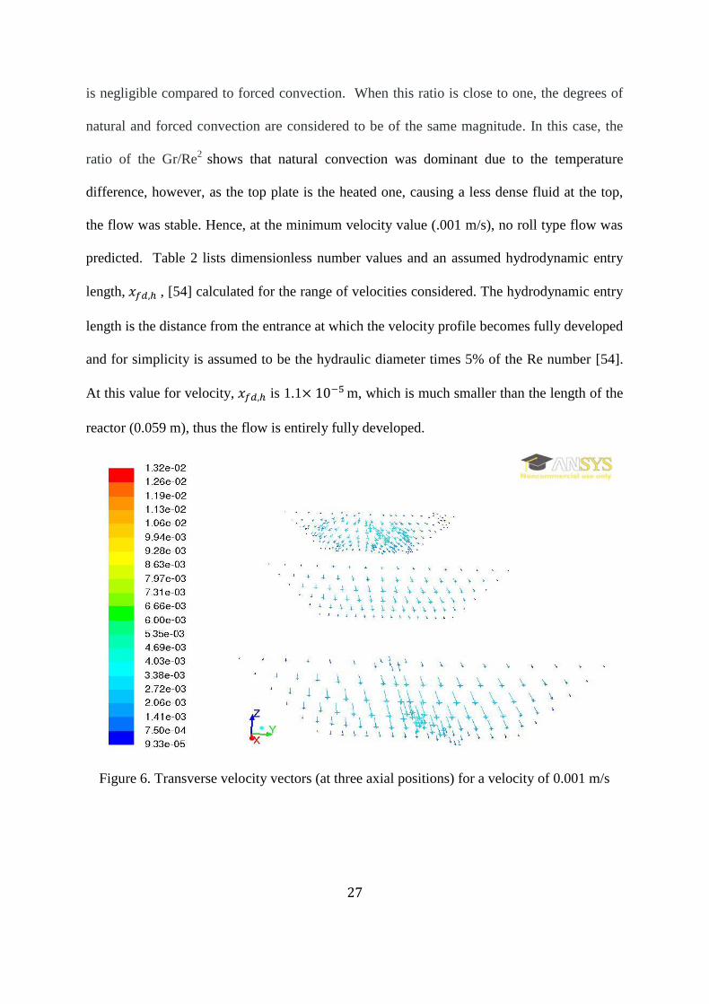
27
is negligible compared to forced convection. When this ratio is close to one, the degrees of
natural and forced convection are considered to be of the same magnitude. In this case, the
ratio of the Gr/Re2
shows that natural convection was dominant due to the temperature
difference, however, as the top plate is the heated one, causing a less dense fluid at the top,
the flow was stable. Hence, at the minimum velocity value (.001 m/s), no roll type flow was
predicted. Table 2 lists dimensionless number values and an assumed hydrodynamic entry
length, , [54] calculated for the range of velocities considered. The hydrodynamic entry
length is the distance from the entrance at which the velocity profile becomes fully developed
and for simplicity is assumed to be the hydraulic diameter times 5% of the Re number [54].
At this value for velocity, is 1.1 m, which is much smaller than the length of the
reactor (0.059 m), thus the flow is entirely fully developed.
Figure 6. Transverse velocity vectors (at three axial positions) for a velocity of 0.001 m/s
28
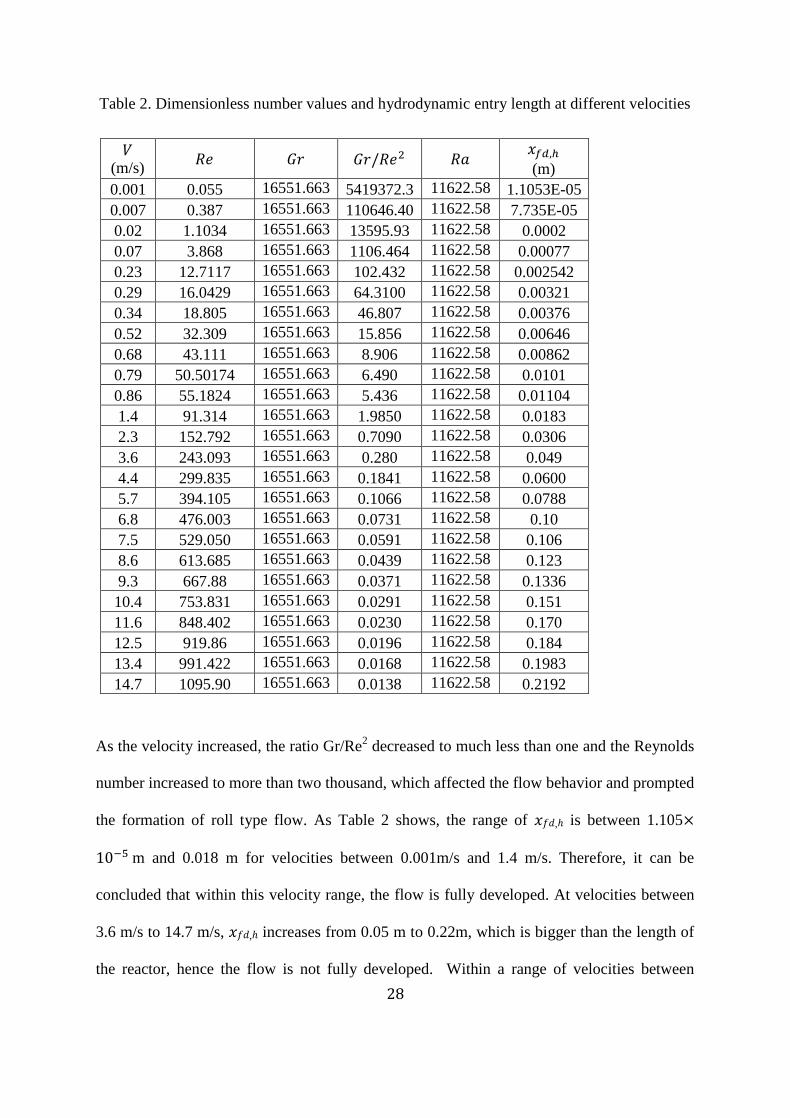
Table 2. Dimensionless number values and hydrodynamic entry length at different velocities
As the velocity increased, the ratio Gr/Re2 decreased to much less than one and the Reynolds
number increased to more than two thousand, which affected the flow behavior and prompted
the formation of roll type flow. As Table 2 shows, the range of ,ℎ is between 1.105
m and 0.018 m for velocities between 0.001m/s and 1.4 m/s. Therefore, it can be
concluded that within this velocity range, the flow is fully developed. At velocities between
3.6 m/s to 14.7 m/s, ,ℎ increases from 0.05 m to 0.22m, which is bigger than the length of
the reactor, hence the flow is not fully developed. Within a range of velocities between
(m/s)
(m)
0.001 0.055 16551.663 5419372.3 11622.58 1.1053E-05
0.007 0.387 16551.663 110646.40 11622.58 7.735E-05
0.02 1.1034 16551.663 13595.93 11622.58 0.0002
0.07 3.868 16551.663 1106.464 11622.58 0.00077
0.23 12.7117 16551.663 102.432 11622.58 0.002542
0.29 16.0429 16551.663 64.3100 11622.58 0.00321
0.34 18.805 16551.663 46.807 11622.58 0.00376
0.52 32.309 16551.663 15.856 11622.58 0.00646
0.68 43.111 16551.663 8.906 11622.58 0.00862
0.79 50.50174 16551.663 6.490 11622.58 0.0101
0.86 55.1824 16551.663 5.436 11622.58 0.01104
1.4 91.314 16551.663 1.9850 11622.58 0.0183
2.3 152.792 16551.663 0.7090 11622.58 0.0306
3.6 243.093 16551.663 0.280 11622.58 0.049
4.4 299.835 16551.663 0.1841 11622.58 0.0600
5.7 394.105 16551.663 0.1066 11622.58 0.0788
6.8 476.003 16551.663 0.0731 11622.58 0.10
7.5 529.050 16551.663 0.0591 11622.58 0.106
8.6 613.685 16551.663 0.0439 11622.58 0.123
9.3 667.88 16551.663 0.0371 11622.58 0.1336
10.4 753.831 16551.663 0.0291 11622.58 0.151
11.6 848.402 16551.663 0.0230 11622.58 0.170
12.5 919.86 16551.663 0.0196 11622.58 0.184
13.4 991.422 16551.663 0.0168 11622.58 0.1983
14.7 1095.90 16551.663 0.0138 11622.58 0.2192

29
0.001 m/s to 1.4 m/s, perturbation of velocity fields at the inlet and middle positions were
observed, but was not considered a major effect for thin topography development as a large
fraction of the flow was swept along the lower boundary. Figure 7 illustrates this for
velocities of (a) 0.07m/s, (b) 0.34 m/s, and (c) 0.86 m/s.
(a)
(b)
30
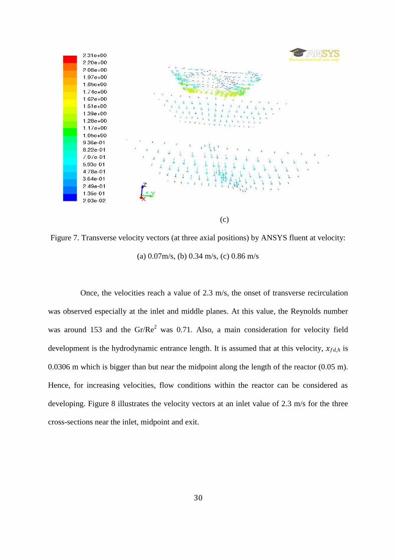
(c)
Figure 7. Transverse velocity vectors (at three axial positions) by ANSYS fluent at velocity:
(a) 0.07m/s, (b) 0.34 m/s, (c) 0.86 m/s
Once, the velocities reach a value of 2.3 m/s, the onset of transverse recirculation
was observed especially at the inlet and middle planes. At this value, the Reynolds number
was around 153 and the Gr/Re2 was 0.71. Also, a main consideration for velocity field
development is the hydrodynamic entrance length. It is assumed that at this velocity, ,ℎ is
0.0306 m which is bigger than but near the midpoint along the length of the reactor (0.05 m).
Hence, for increasing velocities, flow conditions within the reactor can be considered as
developing. Figure 8 illustrates the velocity vectors at an inlet value of 2.3 m/s for the three
cross-sections near the inlet, midpoint and exit.
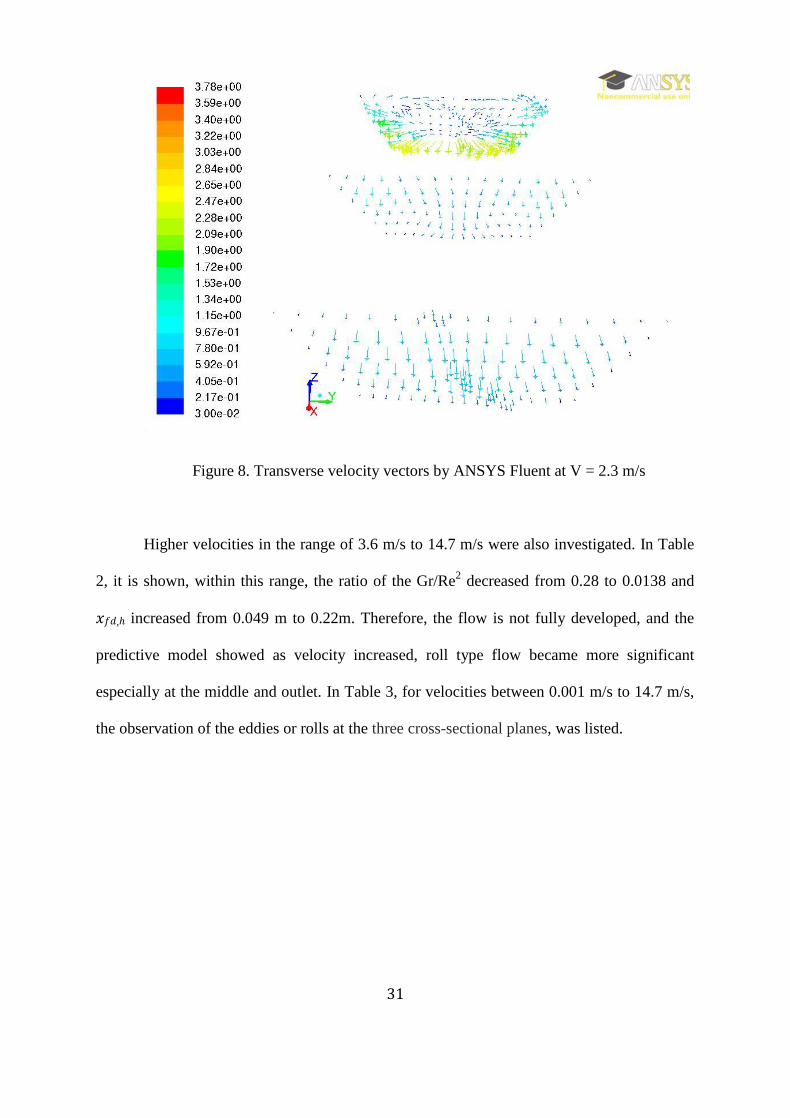
31
Figure 8. Transverse velocity vectors by ANSYS Fluent at V = 2.3 m/s
Higher velocities in the range of 3.6 m/s to 14.7 m/s were also investigated. In Table
2, it is shown, within this range, the ratio of the Gr/Re2 decreased from 0.28 to 0.0138 and
,ℎ increased from 0.049 m to 0.22m. Therefore, the flow is not fully developed, and the
predictive model showed as velocity increased, roll type flow became more significant
especially at the middle and outlet. In Table 3, for velocities between 0.001 m/s to 14.7 m/s,
the observation of the eddies or rolls at the three cross-sectional planes, was listed.

32
Table 3. Observation of roll type flow at μ of 1.663E-5 for different velocities
V (m/s) Eddies or rolls
0.001 Not observed
0.007 Not observed
0.02 Not observed
0.07 Not observed
0.23 Not observed
0.29 Not observed
0.34 Not observed
0.52 Not observed
0.68 Not observed
0.79 Not observed
0.86 Not observed
1.4 Not observed
2.3 Onset of the roll type flow
3.6 Entrance, middle and exit
4.4 Entrance, middle and exit
5.7 Entrance, middle and exit
6.8 Entrance, middle and exit
7.5 Entrance, middle and exit
8.6 Entrance, middle and exit
9.3 Entrance, middle and exit
10.4 Entrance, middle and exit
11.6 Entrance, middle and exit
12.5 Entrance, middle and exit
13.4 Entrance, middle and exit
14.7 Entrance, middle and exit
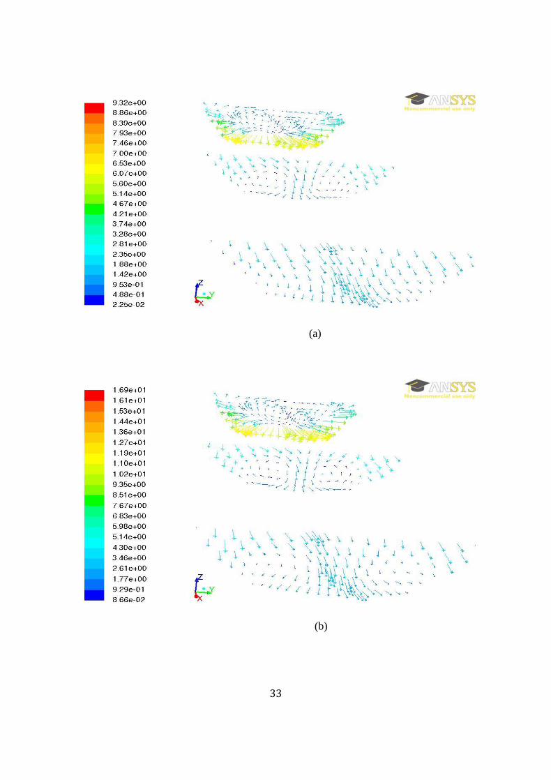
Figure 9 shows illustrations of results for velocity values of 5.7 m/s, 10.4 m/s and
14.7 m/s respectively. At the cross sections close to the inlet and outlet, flow instability was
observed, while at the middle, roll type flow was identified clearly. At these cross-sections, a
secondary flow rotated from the middle and went up along the sidewalls.
At the inlet position, more perturbation was observed then at the mid-plane and the
plane at the outlet position, as rolls started to expand to fill the reactor. The possibility for an
appearance of secondary flow is the slower moving fluid at the corners due to friction
between the fluid and the reactor walls and the faster moving flow at the center of the planes.
33
(a)
(b)
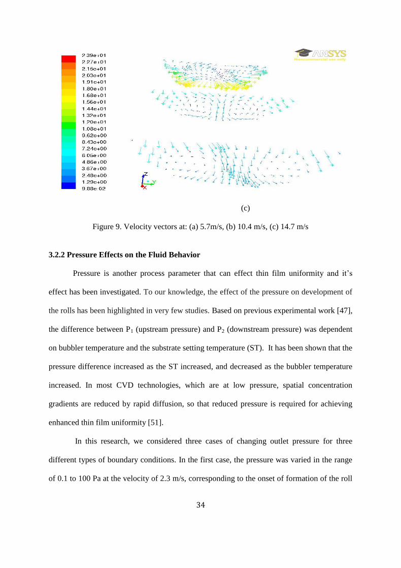
34
(c)
Figure 9. Velocity vectors at: (a) 5.7m/s, (b) 10.4 m/s, (c) 14.7 m/s
3.2.2 Pressure Effects on the Fluid Behavior
Pressure is another process parameter that can effect thin film uniformity and it’s
effect has been investigated. To our knowledge, the effect of the pressure on development of
the rolls has been highlighted in very few studies. Based on previous experimental work [47],
the difference between P1 (upstream pressure) and P2 (downstream pressure) was dependent
on bubbler temperature and the substrate setting temperature (ST). It has been shown that the
pressure difference increased as the ST increased, and decreased as the bubbler temperature
increased. In most CVD technologies, which are at low pressure, spatial concentration
gradients are reduced by rapid diffusion, so that reduced pressure is required for achieving
enhanced thin film uniformity [51].
In this research, we considered three cases of changing outlet pressure for three
different types of boundary conditions. In the first case, the pressure was varied in the range
of 0.1 to 100 Pa at the velocity of 2.3 m/s, corresponding to the onset of formation of the roll
35
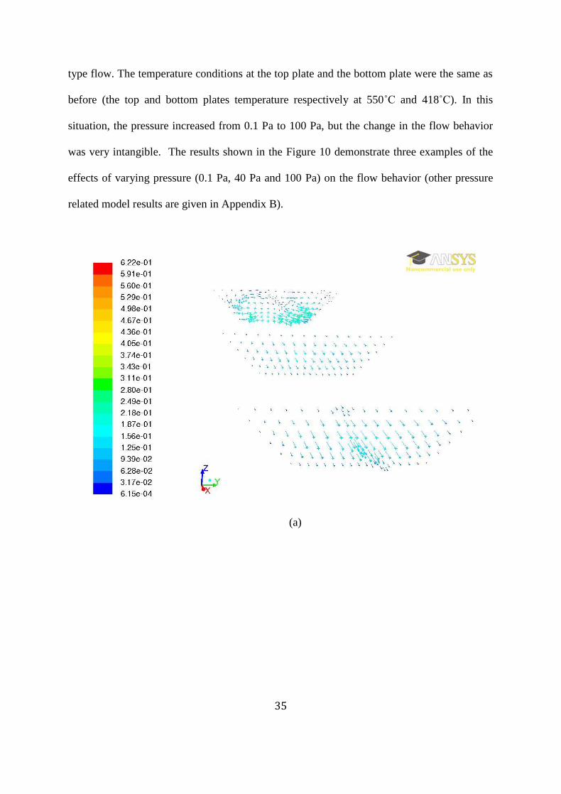
type flow. The temperature conditions at the top plate and the bottom plate were the same as
before (the top and bottom plates temperature respectively at 550˚C and 418˚C). In this
situation, the pressure increased from 0.1 Pa to 100 Pa, but the change in the flow behavior
was very intangible. The results shown in the Figure 10 demonstrate three examples of the
effects of varying pressure (0.1 Pa, 40 Pa and 100 Pa) on the flow behavior (other pressure
related model results are given in Appendix B).
(a)

36
(b)
(c)
Figure 10. The flow behavior at the velocity of 2.3 m/s and d pressures of: (a) 0.1 Pa, (b) 40
Pa, (c) 100 Pa
In the second case, the pressure was changed in the range of 0.1 Pa to 100 Pa at the
velocity of 6.8 m/s. As we discussed before, at this rate, the roll type flow has been seen

37
significantly. With increasing the pressure, a slight variation in the flow pattern took place.
Figure 11 indicates three examples of flow behavior at pressure of .1 Pa, 40 Pa and 100 Pa. It
is shown that the velocity vectors for different pressures are nearly the same.
(a)

38
(b)
(C)
Figure 11. Flow behavior at velocity of 6.8 m/s and pressure of (a) 0.1 Pa, (b) 40 Pa, (c) 100
Pa

39
In the third case, the pressure was changed in the same range and same temperature
but at a velocity of 11.6 m/s. At this rate, the secondary flow has already been observed at
three plates. For enhanced comparison, we modified pressure at a broad range of 0.1 Pa to
100 Pa to evaluate the effect of the pressure on the flow pattern. As the pressure increased,
the change in the flow behavior was very minor. The resulting behavior at three different
pressures is illustrated in Figure 12.
(a)

40
(b)
(c)
Figure 12. Transverse velocity vectors of the flow at the velocity of 11.6 m/s and pressure of:
(a) 0.1Pa, (b) 40 Pa, (c) 100 Pa
41
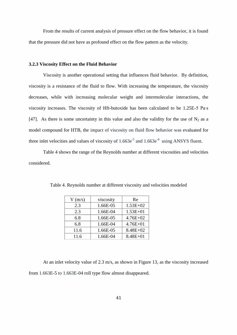
From the results of current analysis of pressure effect on the flow behavior, it is found
that the pressure did not have as profound effect on the flow pattern as the velocity.
3.2.3 Viscosity Effect on the Fluid Behavior
Viscosity is another operational setting that influences fluid behavior. By definition,
viscosity is a resistance of the fluid to flow. With increasing the temperature, the viscosity
decreases, while with increasing molecular weight and intermolecular interactions, the
viscosity increases. The viscosity of Hft-butoxide has been calculated to be 1.25E-5 Pa∙s
[47]. As there is some uncertainty in this value and also the validity for the use of N2 as a
model compound for HTB, the impact of viscosity on fluid flow behavior was evaluated for
three inlet velocities and values of viscosity of 1.663e-5
and 1.663e-4
using ANSYS fluent.
Table 4 shows the range of the Reynolds number at different viscosities and velocities
considered.
Table 4. Reynolds number at different viscosity and velocities modeled
At an inlet velocity value of 2.3 m/s, as shown in Figure 13, as the viscosity increased
from 1.663E-5 to 1.663E-04 roll type flow almost disappeared.
V (m/s) viscosity Re
2.3 1.66E-05 1.53E+02
2.3 1.66E-04 1.53E+01
6.8 1.66E-05 4.76E+02
6.8 1.66E-04 4.76E+01
11.6 1.66E-05 8.48E+02
11.6 1.66E-04 8.48E+01

42
(a)
(b)
Figure 13. Transverse velocity vectors at the velocity of 2.3 m/s and the viscosity of: (a)
1.663E-5 Pa.s, (b) 1.663E-4 Pa.s

43
In the second case for an inlet velocity of 6.8 m/s, the change of viscosity also
brought about a large change in the flow pattern as shown in Figure 14. The range of the
value of the Reynolds number was from 476 to 47. This result has displayed that with
increasing the viscosity, the strength of inertia forces compared to viscous forces was much
larger. As observed before, at this value of the velocity, the secondary flow appeared at the
three cross sections. The model prediction confirmed that when the viscosity increased, the
roll type flow almost disappeared.
(a)

44
(b)
Figure 14. Transversal velocity vectors at the velocity of 6.8 m/s and the viscosity of: (a)
1.663E-5 Pa∙s, (b) 1.663E-4 Pa∙s
In the third situation, the viscosity changed with the same value as before but at a
different inlet velocity (11.6 m/s). The viscosity at these conditions was 1.663E-5 and
1.663E-4. From these values we found that the inertial forces compared to the viscous forces
have negligible effect. When the viscosity increased, the roll type flow has almost
disappeared. Figure 15 illustrates the non-effect of the different viscosities on the flow
pattern at this velocity.

45
(a)
(b)
Figure 15. The numerical modeling at the velocity of 11.6 m/s and the viscosity of: (a)
1.663E-5 Pa∙s, (b) 1.663E-4 Pa∙s

46
3.2.4 Temperature Effects on the Fluid Behavior
Temperature is the last operational setting, which may have an effect on flow
patterns. As illustrated in Boekholt and et.al’s study, temperature gradients cause density
differences and buoyancy driven roll cells in CVD reactors [52]. Simone and coworkers
reported a study on a correlation between the formation of transverse rolls triggered by a
temperature gradient and carbon material growth rate, as well [53]. As the last step in this
modeling effort, the effect of temperature on the flow behavior is presented. As a base case in
the model, the bottom and top plate temperatures were at 145˚C and 250˚C respectively
which match the experimental thin film growth condition showing undulations in film
topography. As discussed before, there were two copper heating rods that were placed on the
top plate to provide heat for the reactor.
In this part, two scenarios have been evaluated: 1) Changing the top plate temperature
and making the bottom plate temperature constant 2) Modifying the bottom plate temperature
and making the top pate temperature constant. In the first case, the velocity was set to values
of 0.34 m/s, 2.3 m/s, and 8.6 m/s and the top plate temperature was increased from 250˚C to
547˚C while the bottom plate temperature was at 145˚C. It is shown through this model that
for an increase of the top plate temperature, the change to the flow behavior was negligible.
Figure 16 shows the predicted model of flow pattern at the velocity of 2.3 m/s and different
temperatures of the top plate using a fixed bottom plate temperature of 145˚C.

47
(a)
(b)
(c)
Figure 16. Velocity vectors using an inlet value of 2.3 m/s and a top plate temperature of: (a)
250˚C, (b) 347˚C, (c) 547˚C

48
Using a larger inlet velocity of 6.8 m/s, it is found that increasing the temperature of
the top plate did not have significant effect on the flow. Figure 17 illustrates the impact of
different temperatures on the flow pattern.
(a)
(b)

49
(c)
Figure 17. Velocity vectors for an inlet velocity 6.8 m/s and a top plate temperature of: (a)
250˚C, (b) 347˚C, (c) 547˚C
Even at the largest inlet velocity considered, 11.6 m/s, increasing the top plate
temperature did not modify the flow pattern. Figure 18 illustrates the flow behavior at three
different top plate temperatures.
(a)

50
(b)
(c)
Figure 18. Transverse velocities at three axial locations for an inlet velocity of 6.8 m/s and top
plate temperatures of: (a) 250˚C, (b) 347˚C, (c) 547˚C
For the second case, the inlet velocity was varied using the same three values: 2.3
m/s, 6.8 m/s and 11.6 m/s, while the top plate temperature was kept at a temperature of
250˚C and the temperature at the bottom plate was increased from 145oC to 380˚C. For the
velocities chosen, increasing the bottom plate temperature did not affect flow pattern. First,
the inlet velocity was kept at the rate of 2.3 m/s, the top plate temperature was at the 250˚C
and the bottom temperature was increased from 145˚C to 380˚C. Figure 19 shows flow
pattern at three different temperatures.

51
(a)
(b)
52
(c)
Figure 19. Transverse velocities at three axial locations for velocity of 2.3 m/s and the
temperature of: (a) 250˚C, (b) 347˚C, (c) 547˚C
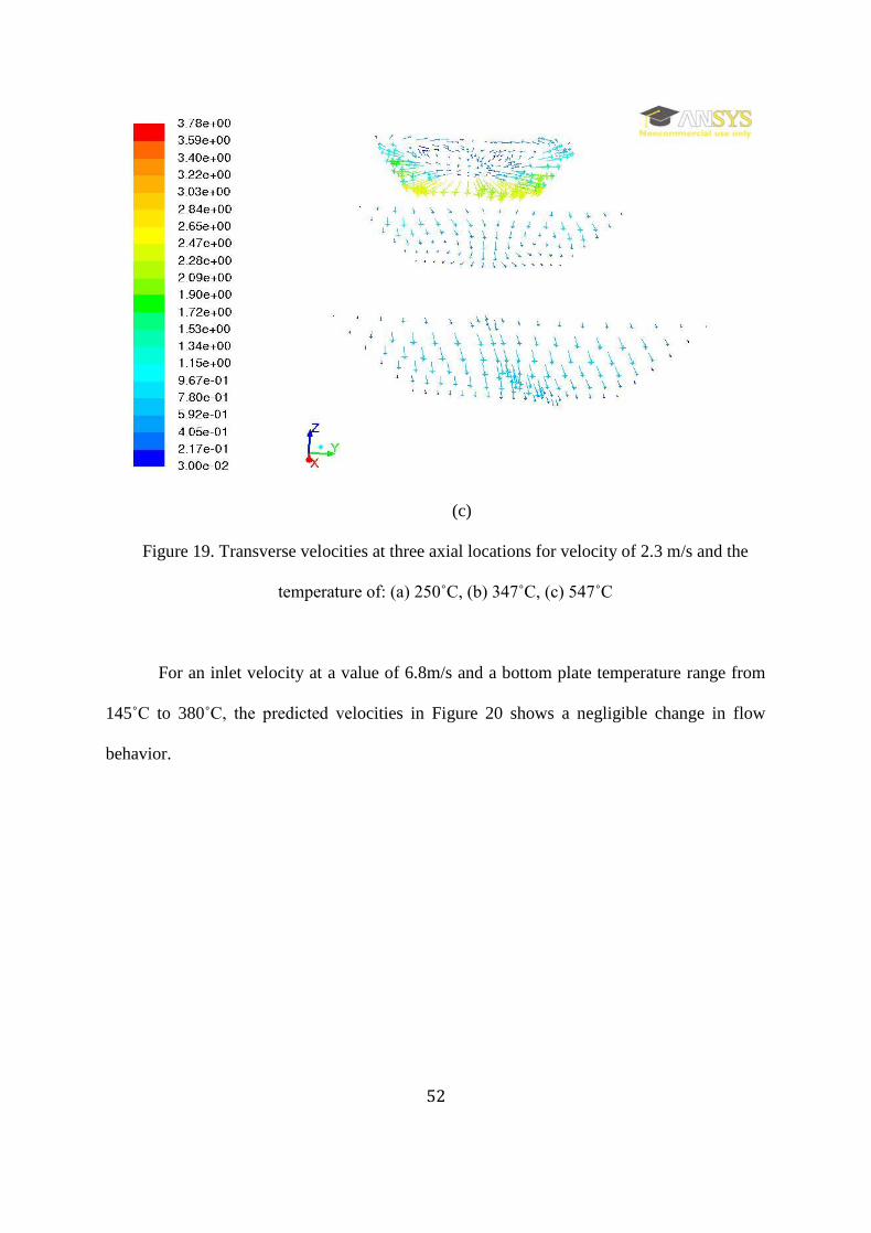
For an inlet velocity at a value of 6.8m/s and a bottom plate temperature range from
145˚C to 380˚C, the predicted velocities in Figure 20 shows a negligible change in flow
behavior.

53
(a)
(b)
54
(c)
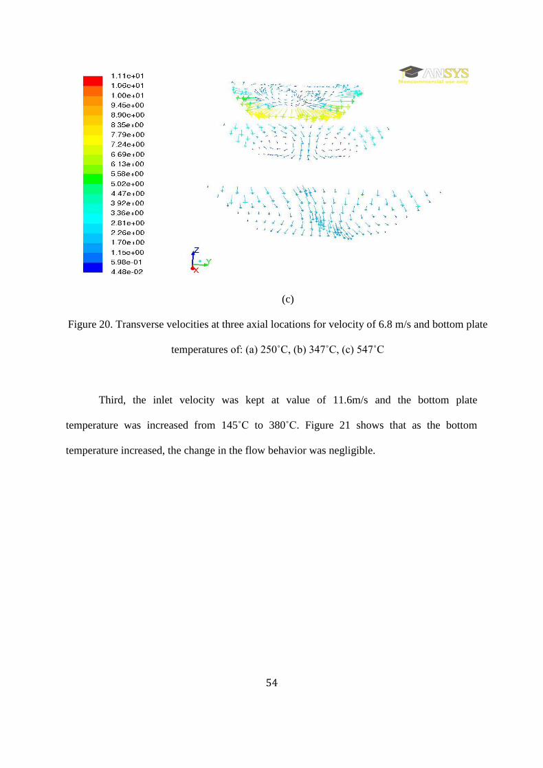
Figure 20. Transverse velocities at three axial locations for velocity of 6.8 m/s and bottom plate
temperatures of: (a) 250˚C, (b) 347˚C, (c) 547˚C
Third, the inlet velocity was kept at value of 11.6m/s and the bottom plate
temperature was increased from 145˚C to 380˚C. Figure 21 shows that as the bottom
temperature increased, the change in the flow behavior was negligible.

55
(a)
(b)
56
(c)
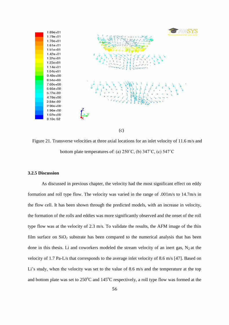
Figure 21. Transverse velocities at three axial locations for an inlet velocity of 11.6 m/s and
bottom plate temperatures of: (a) 250˚C, (b) 347˚C, (c) 547˚C
3.2.5 Discussion
As discussed in previous chapter, the velocity had the most significant effect on eddy
formation and roll type flow. The velocity was varied in the range of .001m/s to 14.7m/s in
the flow cell. It has been shown through the predicted models, with an increase in velocity,
the formation of the rolls and eddies was more significantly observed and the onset of the roll
type flow was at the velocity of 2.3 m/s. To validate the results, the AFM image of the thin
film surface on SiO2 substrate has been compared to the numerical analysis that has been
done in this thesis. Li and coworkers modeled the stream velocity of an inert gas, N2 at the
velocity of 1.7 Pa-L/s that corresponds to the average inlet velocity of 8.6 m/s [47]. Based on
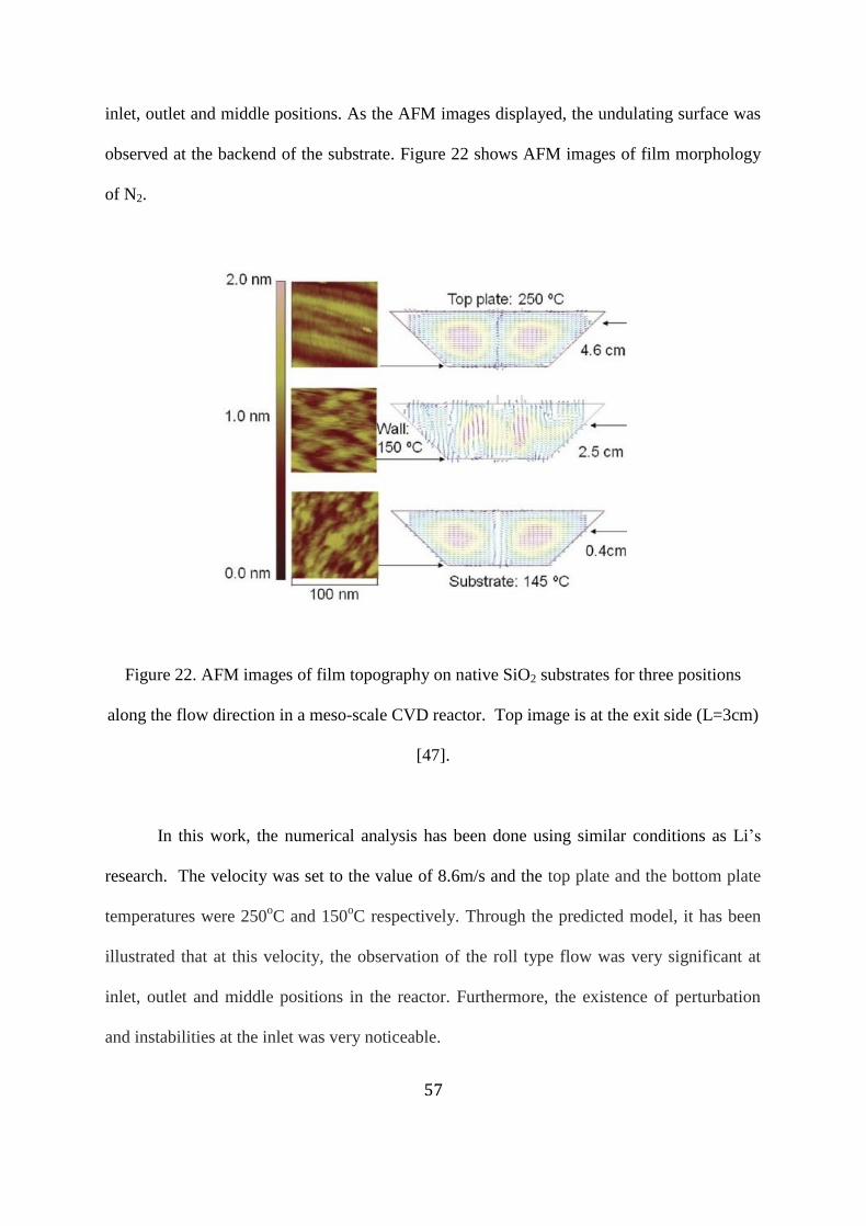
Li’s study, when the velocity was set to the value of 8.6 m/s and the temperature at the top
and bottom plate was set to 250oC and 145
oC respectively, a roll type flow was formed at the
57
inlet, outlet and middle positions. As the AFM images displayed, the undulating surface was
observed at the backend of the substrate. Figure 22 shows AFM images of film morphology
of N2.
Figure 22. AFM images of film topography on native SiO2 substrates for three positions
along the flow direction in a meso-scale CVD reactor. Top image is at the exit side (L=3cm)
[47].
In this work, the numerical analysis has been done using similar conditions as Li’s
research. The velocity was set to the value of 8.6m/s and the top plate and the bottom plate
temperatures were 250oC and 150
oC respectively. Through the predicted model, it has been
illustrated that at this velocity, the observation of the roll type flow was very significant at
inlet, outlet and middle positions in the reactor. Furthermore, the existence of perturbation
and instabilities at the inlet was very noticeable.

58
CHAPTER 4
CONCLUSION AND FUTURE WORK
In this work, a computational analysis was conducted using ANSYS Fluent CFD. The
effect of operational parameters including velocity, pressure, and temperature on the fluid
flow dynamic in a horizontal meso-scale CVD reactor were evaluated. The resulting
prediction represented that the velocity had the most influence on the fluid flow behavior. As
the velocity increased, the roll type flow appeared and increased more significantly. The
onset of a longitudinal vortex roll was at the inlet velocity of 2.3 m/s. As for the pressure and
temperature, their increase did not have much effect on the fluid flow pattern. As a
consequence, the effect of them on the flow regime was less important compared to the
velocity. There are several problems remaining to be solved and needs further analysis. Since
the geometry can be very important parameter to affect flow behavior, a study on the reactor
geometry for providing film uniformity control seems novel and essential. Also, the effect of
the heat flux on the control of the periodicity of the rolls should be studied.
59
REFRENCES
[1]- M.H.-C.Jin, “ The Thin-Film Deposition of Conjugated Molecules for Organic
Electronics” Jom, 81-86 (2008)
[2]- D.R.Cote, S.V. Nguyen, A.K. Stamper, D.S. Armbrust, D. Tobben, R.A. Conti, G.Y.
Lee“, Plasma assisted chemical vapor deposition of dielectric thin films for ULSI
semiconductor circuits” Journal of Research and Development, 43, 1-2, 5-38(1999)
[3]- C. Gaire, S. Rao , M. Riley, L. Chen, A. Goyal, S. Lee, I. Bhat, T.-M. Lu, G.-C. Wang,
“Epitaxialgrowth of CdTe thin film on cube-textured Ni by metal-organic chemical
vapor deposition”, Thin Solid Films 520, 1862–1865(2012)
[4]- R.Wang, R.Ma, “ An integrated model for halide chemical vapor deposition of silicon
carbide epitaxial films”, Journal of Crystal Growth, 310, 18, 4248–4255 (2008)
[5]- J. KF, “Flow phenomena in chemical vapor deposition of thin films”, Anne RevFluid
Mech, 23, 297-232 (1991)
[6]- J.Robertson, “High dielectric constant gate oxides for metal oxide Si transistors”,
Reports on Progress Physics, 69,317 (2006)
[7]- G.Tsutsui,T.Hiramoto, “Mobility and Threshold-Voltage Comparison Between (110)-
and (100)-Oriented Ultrathin- “IEEE Transactions on
Electron Devices”,53,2582 (2006)
[8]- A. Khodakov, B. Olthof, A.T. Bell, E. Iglesia, “Structure and Catalytic Properties of
Supported Vanadium Oxides: Support Effects on Oxidative Dehydrogenation Reactions
“ J. Catalysis, 181, 205 (1999)
[9]-J.Tsaur, K.Onodera,T.Kobayashi,Z.J.Wang,S.Heisig,R.Maeda, “Broadband MEMS shunt
switches using PZT/HfO2 multi-layered high k dielectrics for high switching isolation”,
Sensors and Actuators, 121, 275 (2005)
[10]-Y. Zhao, T. Wang, D. Zhang, J. Shao, Z. Fan, “Laser conditioning and multi-shot laser
damage accumulation effects of HfO2/SiO2 antireflective coatings”, Surface of Science,
245, 335 (2005)
[11]- J.M. Hughes-Oliver, J. Lu, J.C. Davis and R. S. Gyurcsik, “Achieving Uniformity in a
Semiconductor Fabrication Process Using Spatial Modeling”, Journal of the American
Statistical Association, 93,441, 36-45(1998)
[12]- F. Fau-Canillac and F. Maury, “Control of the uniformity of thickness of Ni thin films

60
deposited by low pressure chemical vapor deposition”, Surface mill Coatings
Technology. 64, 21- 27 (1994)
[13]- I. Mahawili, “Chemical vapor deposition reactor and method of operation”, United
States Patent, P. N. 4,993, 358
[14]- A.C. Jones, M.L. Hitchman, “ Chemical Vapor Deposition: precursor, processes and
applications”, Royal society of chemistry, 2008
[15]-K. PK, C.IM “Fluid Mechanic”, 2nd
ed, San Diego, CA: Academic Press, 2002.
[16]- R. L. Mahajan, "Transport Phenomena in Chemical Vapor-Deposition
Systems,"Advances in Heat Transfer, Academic Press, 28, 339-425(1996)
[17]- D. B. Fraser, "Metallization," VLSI Technology, S. M. Sze, Ed., p. 347, McGraw-Hill,
New York, 1983
[18]-C. T. Foxon, "Principles of Molecular Beam Epitaxy," Handbook of CrystalGrowth, D.
Hurle, Ed, vol. 3a, Elsevier, Amsterdam, 1994
[19]- K.F., E.O. Einset, and D.I. Fotiadis, “Flow Phenomena in Chemical Vapor Deposition
of Thin Films”, Annual Review of Fluid Mechanics23197-232 (1991)
[20]- Y. Jaluria,” Fluid Flow Phenomena in Materials Processing—The 2000 Freeman
Scholar Lecture”, Journal of Fluids Engineering, 123, 173-210 (2001)
[21]- R.Vuthaluru, M.Tade, H.Vuthaluru, Y.Tsvetnenko, L.Evans, J.Milne, “Application of
CFD modeling to investigate fluidized limestone reactors for the remediation of acidic
drainage waters”, Chemical Engineering Journal 149,162–172 (2009)
[22]- R. I. Singh, A. Brink, M. Hupa, “ CFD modeling to study fluidized bed combustion and
gasification”, Applied Thermal Engineering 52, 585-614 (2013)
[23]- D. Vallespin, K.J. Badcock, A. Da Ronch, M.D. White, P. Perfect, M. Ghoreyshi,
“Computational fluid dynamics framework for aerodynamic model assessment”,
Progress in Aerospace Sciences 52, 2–18 (2012)
[24]- S. Balaji, Juan Du, C.M. White, B. Erik Ydstie, “Multi-scale modeling and control of
fluidized beds for the production of solar grade silicon”, Powder Technology 199, 23–
(2010)
[25]- Hugo O. Pierson, “ Hand Book Of Chemical Vapor Deposition (CVD)”, 1992
[26]- N. Kockmann, O. Brand, G. K. Fedder, C. Hierold, J. G. Korvink, and O. Tabata,
“Advanced Micro Nano-systems: Fundamentals, Devices, Fabrication, and
Applications” Weinheim, Germany: WILEY-VCH Verlag GmbH Co. KGaA, 2006.
[27]- A.Dessimoz, L. Cavinb, A. Renken, L. Kiwi-Minsker, “Liquid–liquid two-phase flow
patterns and mass transfer characteristics in rectangular glass micro reactors”, Chemical
Engineering Science, 63, 4035-4044 (2008)

61
[28]- G.Kolb, V. Hessel, “Micro-structured reactors for gas phase reactions”, Chemical
Engineering Journal, 98,1–38 (2004)
[29]- Y. Okubo, T. Maki, F. Nakanishi, T. Hayashi and K. Mae, “Precise control of polymer
particle properties using droplets in the micro channel”, Chemical Engineering Science,
65, 386-391 (2010)
[30]- Y. Okubo, T. Maki, N. Aoki, T. Hong Khoo, Y. Ohmukai, K. Mae, “Liquid–liquid
extraction for efficient synthesis and separation by utilizing micro spaces”, Chemical
Engineering Science, 63, 4070-4077, (2008)
[31]- X. Zhang, S. Stefanick, and F.J. Villani, “Application of Micro-reactor Technology in
Process Development”, Organic Process Research & Development, 8, 455−460 (2004)
[32]- W.Wang, W.Ge, N.Yang and J.Li, “Meso-Scale Modeling—The Key Contents to
Multi-Scale CFD Simulation”
[33]- S. Patnaik, R.A. Brown, “Hydrodynamic dispersion in rotating-disk OMVPE reactors:
numerical simulation and experimental measurements”, Journal of Crystal growth, 96,
153-174 (1989)
[34]- Harry.M, Klavis F. j ,Complex flow phenomena in MOCVD Reactors,
[35]- At.Dhanorker and T.Özel, “An experimental and modeling study on meso/micro end
milling process” American Society of Mechanical Engineering, 1-8 (2006)
[36]- Katsuki .K, Shigeharu.M and Hideaki.M, “Development of A Mkrochannel Catalytic
Reactor System”,
[37]- D.I. Fotiadis, S.Kieda, and K.F. Jensen, “ Transport phenomena in vertical reactors for
metal organic vapor phase epitaxy”, Journal of crystal growth, 102,441-470 (1990)
[38]- S. Patnaik, R.A. Brown, C.A. Wang,” Hydrodynamic dispersion in rotating-disk omvpe
reactors: Numerical simulation and experimental measurements”, Journal of crystal
growth, 96,153–174 (1981)
[39]- E.P. Visser, C.R. Kleijn, C.A.M. Govers, C.J. Hoogendoorn, L.J. Giling, “Return flows
in horizontal MOCVD reactors studied with the use of TiO2 particle injection and
numerical calculations” journal of crystal growth, 929-946, 94 (1989)
[40]-T.M. Makhviladze, A.V. Martjushenko, “Several aspects of the return flows formation
in horizontal CVD reactors”, International Journal of Heat and Mass Transfer, 41,
2529-2536 (1998)
[41]- H.V.Santen, C.R. Kleijn,H.V. Akker, “ On multiple stability of mixed-convection flows
in a chemical vapor deposition reactor” International Journal of Heat and Mass
Transfer, 44, 659-672 (2001)
[42]- C.R. Kleijn, K.J. Kuijlaars, M. Okkerse, H. van Santen and H.E.A. van den Akker,
“Some recent developments in chemical vapor deposition process and equipment

62
modeling”, Journal of De physique IV, 9, 8-132(1999)
[43]- P. Gadgil, “ Optimization of a stagnation point flow reactor design for metal organic
chemical vapor deposition by flow visualization”, Journal of Crystal Growth, 134, 302-
312 (1993)
[44]- M.C.Kim, j.S.Baik, I.G.Hwang, D-Y.Yoon, C.K. Choi, “Buoyancy-driven convection
in plane Poiseuille flow”,
[45]- T.S. Chang, M.C.Hsiao, “Computation of three-dimensional flow and thermal fields in
a model horizontal chemical vapor deposition reactor”
[46]- T.M.Makhviladz, A.V.Martjushenko, “Several aspects of the return flows formation in
horizontal CVD reactors”
[47]- K.Li, L. Zhang, D.A. Dixon, T.M. klein, “ Undulating Topograghy of HfO2 Thin Films
Deposited in a Mesoscale Reactor Using Hafnium (IV) tert Butoxide” AlChE Jounal,
57(11), 2989-2996(2011)
[48]- S. Sayan, S. Aravamudhan, B. W. Busch, W. H. Schulte, F. Cosandey, G. D. Wilk, T.
Gustafsson, E. Garfunkel, “Chemical vapor deposition of HfO2 films on Si„100”,
Journal of vacuum and science technology, 20(2), 507-512, (2002)
[49]- “ANSYS Fluent 12 theorygide”, 2009
[50]- http://hyperphysics.phy-astr.gsu.edu/hbase/kinetic/menfre.html
[51]- S.P. Vanka, G. Luo, N.G. Glumac, “Parametric effects on thin film growth and
uniformity in an atmospheric pressure impinging jet CVD reactor”, Journal of crystal
growth, 267,22-34 (2004)
[52]- M. Boekholt, K.F. Jensen, and W. Richter “ Flow and heat transfer in CVD reactors:
Comparison of Raman temperature measurements and finite element model predictions”
Journal of crystal growth, 100, 577-599 (1990)
[53]- S. Mussoa, S. Porro, M. Rovere, M. Giorcelli, A. Tagliaferro “Fluid dynamic analysis
of gas flow in a thermal-CVD system designed for growth of carbon nanotubes”,
Journal of Crystal Growth 310, 477–483 (2008)
[54]-T.L. Bergman, A.S. Lavine, F. P. Incropera, D.P. Dewitt, “ Fundamentals of heat and
mass transfer” (2011)
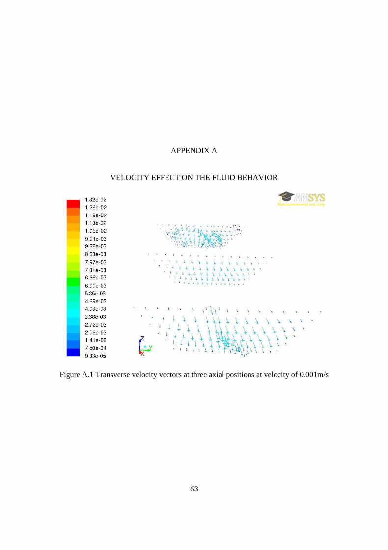
63
APPENDIX A
VELOCITY EFFECT ON THE FLUID BEHAVIOR
Figure A.1 Transverse velocity vectors at three axial positions at velocity of 0.001m/s
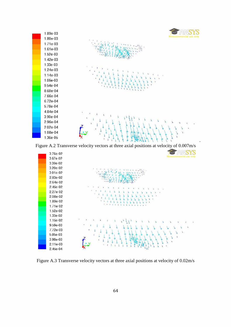
64
.
Figure A.2 Transverse velocity vectors at three axial positions at velocity of 0.007m/s
Figure A.3 Transverse velocity vectors at three axial positions at velocity of 0.02m/s

65
Figure A.4 Transverse velocity vectors at three axial positions at velocity of 0.07m/s
Figure A.5Transverse velocity vectors at three axial positions at velocity of 0.23m/s

66
Figure A.6 Transverse velocity vectors at three axial positions at velocity of 0.29m/s
Figure A.8 Transverse velocity vectors at three axial positions at velocity of 0.34 m/s

67
Figure A.9 Transverse velocity vectors at three axial positions at velocity of 0.52 m/s
Figure A.10 Transverse velocity vectors at three axial positions at velocity of 0.68 m/s

68
Figure A.11 Transverse velocity vectors at three axial positions at velocity of 0.79 m/s
Figure A.12Transverse velocity vectors at three axial positions at velocity of 0.86 m/s

69
Figure A.13 Transverse velocity vectors at three axial positions at velocity of 1.4m/s
Figure A.14 Transverse velocity vectors at three axial positions at velocity of 2.3 m/s

70
Figure A.15 Transverse velocity vectors at three axial positions at velocity of 3.6 m/s
Figure A.16 Transverse velocity vectors at three axial positions at velocity of 4.4 m/s

71
Figure A.17 Transverse velocity vectors at three axial positions at velocity of 5.7m/s
Figure A.18 Transverse velocity vectors at three axial positions at velocity of 6.8 m/s

72
Figure A.19 Transverse velocity vectors at three axial positions at velocity of 7.5 m/s
Figure A.20 Transverse velocity vectors at three axial positions at velocity of 8.6 m/s

73
Figure A.21 Transverse velocity vectors at three axial positions at velocity of 9.3 m/s
Figure A.22 Transverse velocity vectors at three axial positions at velocity of 10.4 m/s

74
Figure A.23 Transverse velocity vectors at three axial positions at velocity of 11.6 m/s
Figure A.24 Transverse velocity vectors at three axial positions at velocity of 12.5 m/s

75
Figure A.25 Transverse velocity vectors at three axial positions at velocity of 13.4 m/s
Figure A.26 Transverse velocity vectors at three axial positions at velocity of 14.7 m/s
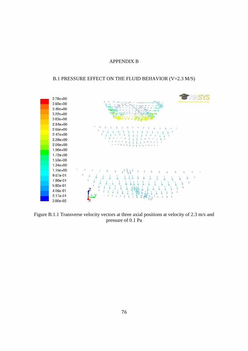
76
APPENDIX B
B.1 PRESSURE EFFECT ON THE FLUID BEHAVIOR (V=2.3 M/S)
Figure B.1.1 Transverse velocity vectors at three axial positions at velocity of 2.3 m/s and
pressure of 0.1 Pa

77
Figure B.1.2 Transverse velocity vectors at three axial positions at velocity of 2.3 m/s and
pressure of 5 Pa
Figure B.1.3 Transverse velocity vectors at three axial positions at velocity of 2.3 m/s and
pressure of 10 Pa

78
Figure B.1.4 Transverse velocity vectors at three axial positions at velocity of 2.3 m/s and
pressure of 20 Pa
Figure B.1.5 Transverse velocity vectors at three axial positions at velocity of 2.3 m/s and
pressure of 40 Pa

79
Figure B.1.6 Transverse velocity vectors at three axial positions at velocity of 2.3 m/s and
pressure of 60 Pa
Figure B.1.7 Transverse velocity vectors at three axial positions at velocity of 2.3 m/s and
pressure of 80 Pa

80
Figure B.1.8 Transverse velocity vectors at three axial positions at velocity of 2.3 m/s and
pressure of 100 Pa
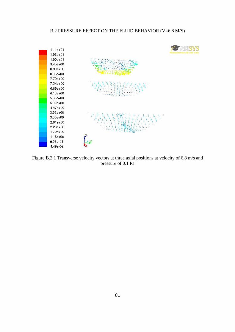
81
B.2 PRESSURE EFFECT ON THE FLUID BEHAVIOR (V=6.8 M/S)
Figure B.2.1 Transverse velocity vectors at three axial positions at velocity of 6.8 m/s and
pressure of 0.1 Pa
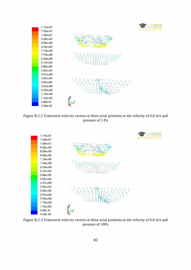
82
Figure B.2.2 Transverse velocity vectors at three axial positions at the velocity of 6.8 m/s and
pressure of 5 Pa
Figure B.2.3 Transverse velocity vectors at three axial positions at the velocity of 6.8 m/s and
pressure of 10Pa
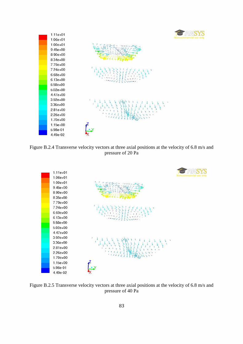
83
Figure B.2.4 Transverse velocity vectors at three axial positions at the velocity of 6.8 m/s and
pressure of 20 Pa
Figure B.2.5 Transverse velocity vectors at three axial positions at the velocity of 6.8 m/s and
pressure of 40 Pa

84
Figure B.2.6 Transverse velocity vectors at three axial positions at the velocity of 6.8 m/s and
pressure of 60 Pa
Figure B.2.7 Transverse velocity vectors at three axial positions at the velocity of 6.8 m/s and
pressure of 80Pa

85
Figure B.2.8 Transverse velocity vectors a8t three axial positions at the velocity of 6.8 m/s
and pressure of 100 Pa

86
B.3 PRESSURE EFFECT ON THE FLUID BEHAVIOR (V=11.6 M/S)
Figure B.3.1 Transverse velocity vectors at three axial positions at velocity of 11.6 m/s and
pressure of 0.1 Pa

87
Figure B.3.2 Transverse velocity vectors at three axial positions at velocity of 11.6 m/s and
pressure of 5 Pa
Figure B.3.3 Transverse velocity vectors at three axial positions at velocity of 11.6 m/s and
pressure of 10 Pa

88
Figure B.3.4 Transverse velocity vectors at three axial positions at velocity of 11.6 m/s and
pressure of 20 Pa
Figure B.3.5 Transverse velocity vectors at three axial positions at velocity of 11.6 m/s and
pressure of 40 Pa

89
Figure B.3.6 Transverse velocity vectors at three axial positions at velocity of 11.6 m/s and
pressure of 60 Pa
Figure B.3.67 Transverse velocity vectors at three axial positions at velocity of 11.6 m/s and
pressure of 80 Pa

90
Figure B.3.8 Transverse velocity vectors at three axial positions at velocity of 11.6 m/s and
pressure of 100 Pa


