
COMPARISON OF DIFFERENT KALMAN FILTERS FOR APPLICATIONTO MOBILE ROBOTICS
by
Suraj RavichandranA Thesis
Submitted to theGraduate Faculty
ofGeorge Mason UniversityIn Partial fulfillment of
The Requirements for the Degreeof
Master of ScienceElectrical Engineering
Committee:
Dr. Gerald Cook, Thesis Director
Dr. Janos Gertler, Committee Member
Dr. Jill K. Nelson, Committee Member
Dr. Andre Manitius, Chairman, Departmentof Electrical & Computer Engineering
Dr. Kenneth S. Ball, Dean, Volgenau Schoolof Engineering
Date: Spring Semester 2014George Mason UniversityFairfax, VA

Comparison of Different Kalman Filters for Applicationto Mobile Robotics
A thesis submitted in partial fulfillment of the requirements for the degree ofMaster of Science at George Mason University
By
Suraj RavichandranBachelor of EngineeringMumbai University, 2011
Director: Dr. Gerald Cook, ProfessorDepartment of Electrical & Computer Engineering
Spring Semester 2014George Mason University
Fairfax, VA

Acknowledgments
I am forever in debt of Dr. Cook, without whose support neither would I have come upwith this topic, let alone have known about its existence in the first place. Thank you forbearing with me, and for believing that I would FINALLY finish my thesis. Without youto guide me, I would be just another masters student who would have ended up regrettingtaking up this endeavor of Graduate School. . .
A special thanks to Dr. Janos Gertler, who empathised with my situation and took thetime to painstakingly find even the minute mistakes/typos in my thesis, even during theholidays. Your comments and suggestions rendered have given my thesis a professional andtechnical edge.
It was Dr Jill Nelson’s ingenious idea of taking up special registration, which allowed me todefend my thesis an entire semester earlier. I owe you the time I saved as well as the peaceof mind that I could only afford because of the special registration option. I also appreciateyou agreeing to be on my committee on such short notice and bailing me out of troubleonce more.
And finally, any research without proper documentation and administrative protocol ismeaningless. Without the help of Patricia Sahs and Jammie Chang I would have beenrunning from pillar to post clueless trying to comprehend what paperwork is needed andwhat are the deadlines. They have been most helpful and co-operative in my time of need.I am in debt of both of you for all the assistance and guidance that you provided, like thefoundation of a building providing constant support whilst staying out of the limelight.
iii

Table of Contents
Page
List of Tables . . . . . . . . . . . . . . . . . . . . . . . . . . . . . . . . . . . . . . . . vi
List of Figures . . . . . . . . . . . . . . . . . . . . . . . . . . . . . . . . . . . . . . . . vii
List of Abbreviations . . . . . . . . . . . . . . . . . . . . . . . . . . . . . . . . . . . . viii
Abstract . . . . . . . . . . . . . . . . . . . . . . . . . . . . . . . . . . . . . . . . . . . ix
1 Introduction . . . . . . . . . . . . . . . . . . . . . . . . . . . . . . . . . . . . . . 1
1.1 Limitations of the Linear Kalman Filter . . . . . . . . . . . . . . . . . . . . 1
1.1.1 An Initial yet robust fix – The Extended Kalman Filter . . . . . . . 2
1.2 The Ultimate Solution – Particle Filter . . . . . . . . . . . . . . . . . . . . . 4
1.2.1 Trouble in Paradise – Computationally Prohibitive . . . . . . . . . . 5
1.3 Why stick to the Kalman Filter? . . . . . . . . . . . . . . . . . . . . . . . . 5
1.3.1 Kalman Filter Derivatives . . . . . . . . . . . . . . . . . . . . . . . . 6
2 Mobile Robot Dynamics . . . . . . . . . . . . . . . . . . . . . . . . . . . . . . . . 7
2.1 Mobile Robot Setup . . . . . . . . . . . . . . . . . . . . . . . . . . . . . . . 7
2.1.1 Robot Kinematics in Local Coordinates . . . . . . . . . . . . . . . . 8
2.1.2 Rotation to Earth Coordinates . . . . . . . . . . . . . . . . . . . . . 10
2.2 Steering Control Law . . . . . . . . . . . . . . . . . . . . . . . . . . . . . . . 10
2.3 Choice of Method for Numerical Integration . . . . . . . . . . . . . . . . . . 11
2.3.1 Euler’s Method . . . . . . . . . . . . . . . . . . . . . . . . . . . . . . 11
2.3.2 Runge Kutta . . . . . . . . . . . . . . . . . . . . . . . . . . . . . . . 13
2.4 Sensors . . . . . . . . . . . . . . . . . . . . . . . . . . . . . . . . . . . . . . 14
3 State Estimation using the EKF . . . . . . . . . . . . . . . . . . . . . . . . . . . 15
3.1 EKF Derivation for Mobile Robot . . . . . . . . . . . . . . . . . . . . . . . 15
3.1.1 The Final State Space Representation . . . . . . . . . . . . . . . . . 18
3.1.2 Final Flow Algorithm for the EKF . . . . . . . . . . . . . . . . . . . 20
3.2 EKF Derivatives . . . . . . . . . . . . . . . . . . . . . . . . . . . . . . . . . 20
3.2.1 The Iterated Extended Kalman Filter . . . . . . . . . . . . . . . . . 21
3.3 A look on Statistical Linearization Methods for the Non-Linear Kalman Filter 23
3.3.1 The Achilles heel of this Approach! . . . . . . . . . . . . . . . . . . . 24
3.3.2 Monte-Carlo Kalman Filter . . . . . . . . . . . . . . . . . . . . . . . 24
iv

4 State Estimation using the UKF . . . . . . . . . . . . . . . . . . . . . . . . . . . 28
4.1 Introduction to the Sigma Point Approach . . . . . . . . . . . . . . . . . . . 28
4.2 The Unscented Transform . . . . . . . . . . . . . . . . . . . . . . . . . . . . 30
4.3 The Scaled Unscented Transform . . . . . . . . . . . . . . . . . . . . . . . . 31
4.4 Tuning the Weights . . . . . . . . . . . . . . . . . . . . . . . . . . . . . . . . 33
4.5 The UKF Algorithm . . . . . . . . . . . . . . . . . . . . . . . . . . . . . . . 34
4.5.1 Augmented UKF . . . . . . . . . . . . . . . . . . . . . . . . . . . . . 34
4.5.2 Non-augmented UKF . . . . . . . . . . . . . . . . . . . . . . . . . . 37
4.6 The Square Root UKF . . . . . . . . . . . . . . . . . . . . . . . . . . . . . . 38
4.6.1 The SR-UKF Filter Algorithm . . . . . . . . . . . . . . . . . . . . . 40
4.7 An Illustrative comparison of the UKF with the EKF . . . . . . . . . . . . 43
5 Results: Simulation and Analysis . . . . . . . . . . . . . . . . . . . . . . . . . . . 45
5.1 Matlab Simulation . . . . . . . . . . . . . . . . . . . . . . . . . . . . . . . . 45
5.1.1 Environment Variables . . . . . . . . . . . . . . . . . . . . . . . . . . 46
5.2 Graphs . . . . . . . . . . . . . . . . . . . . . . . . . . . . . . . . . . . . . . . 48
5.2.1 EKF Path 1 . . . . . . . . . . . . . . . . . . . . . . . . . . . . . . . . 49
5.2.2 EKF Path 2 . . . . . . . . . . . . . . . . . . . . . . . . . . . . . . . . 50
5.2.3 IEKF Path 1 . . . . . . . . . . . . . . . . . . . . . . . . . . . . . . . 51
5.2.4 IEKF Path 2 . . . . . . . . . . . . . . . . . . . . . . . . . . . . . . . 52
5.2.5 UKF Path 1 . . . . . . . . . . . . . . . . . . . . . . . . . . . . . . . 53
5.2.6 UKF Path 2 . . . . . . . . . . . . . . . . . . . . . . . . . . . . . . . 54
5.2.7 Accuracy and Computational Costs (Time) . . . . . . . . . . . . . . 55
5.3 Verification of the UKF Implementation . . . . . . . . . . . . . . . . . . . . 56
5.3.1 Testing the Unscented Transform . . . . . . . . . . . . . . . . . . . . 56
5.4 Averaging over multiple runs . . . . . . . . . . . . . . . . . . . . . . . . . . 62
5.5 Inference . . . . . . . . . . . . . . . . . . . . . . . . . . . . . . . . . . . . . . 63
5.6 Future Scope . . . . . . . . . . . . . . . . . . . . . . . . . . . . . . . . . . . 63
A Matlab Codes . . . . . . . . . . . . . . . . . . . . . . . . . . . . . . . . . . . . . 64
Bibliography . . . . . . . . . . . . . . . . . . . . . . . . . . . . . . . . . . . . . . . . . 101
v

List of Tables
Table Page
5.1 Comparison Table for Path 1 . . . . . . . . . . . . . . . . . . . . . . . . . . 55
5.2 Comparison Table for Path 2 . . . . . . . . . . . . . . . . . . . . . . . . . . 56
5.3 EKF v/s UKF MSE averaged over 1000 runs . . . . . . . . . . . . . . . . . 63
vi

List of Figures
Figure Page
2.1 Front-Wheel steered robot schematic diagram[1] . . . . . . . . . . . . . . . 8
3.1 EKF Process Flow Diagram . . . . . . . . . . . . . . . . . . . . . . . . . . . 20
4.1 The transformation of sigma points through a nonlinear function[2] . . . . . 29
4.2 Comparison of mean and covariance sampling by Monte-Carlo Sampling,
EKF and UKF[3] . . . . . . . . . . . . . . . . . . . . . . . . . . . . . . . . . 44
5.1 EKF Plot for True v/s Estimated Robot Trajectory . . . . . . . . . . . . . 49
5.2 EKF Plot for True v/s Estimated Heading Angle . . . . . . . . . . . . . . . 49
5.3 EKF Plot for True v/s Estimated Robot Trajectory . . . . . . . . . . . . . 50
5.4 EKF Plot for True v/s Estimated heading Angle . . . . . . . . . . . . . . . 50
5.5 IEKF Plot for True v/s Estimated Robot Trajectory . . . . . . . . . . . . . 51
5.6 IEKF Plot for True v/s Estimated Heading Angle . . . . . . . . . . . . . . 51
5.7 IEKF Plot for True v/s Estimated Robot Trajectory . . . . . . . . . . . . . 52
5.8 IEKF Plot for True v/s Estimated heading Angle . . . . . . . . . . . . . . . 52
5.9 UKF Plot for True v/s Estimated Robot Trajectory . . . . . . . . . . . . . 53
5.10 UKF Plot for True v/s Estimated Heading Angle . . . . . . . . . . . . . . 53
5.11 UKF Plot for True v/s Estimated Robot Trajectory . . . . . . . . . . . . . 54
5.12 UKF Plot for True v/s Estimated heading Angle . . . . . . . . . . . . . . . 54
5.13 Error Covariance Ellipsoid: Sigma points around the mean with α = 0.5 . . 59
5.14 Error Covariance Ellipsoid: Sigma points around the mean with α = 0.9 . . 60
vii

List of Abbreviations
EKF Extended Kalman FilterIEKF Iterated Extended Kalman FilterUKF Unscented Kalman FilterPDF Probability Density FunctionMSE Mean Squared ErrorMCKF Monte-Carlo Kalman FilterSR-UKF Square-Root Unscented Kalman FilterRK Runge Kutta
viii

Abstract
COMPARISON OF DIFFERENT KALMAN FILTERS FOR APPLICATIONTO MOBILE ROBOTICS
Suraj Ravichandran, MS
George Mason University, 2014
Thesis Director: Dr. Gerald Cook
The problem of state estimation of the mobile robot’s trajectory being a nonlinear one, the
intent of this thesis is to go beyond the realm of the basic Extended Kalman Filter(EKF)
and study the more recent nonlinear Kalman Filters for their application to the problem at
hand. The various filters that I employ in this study are:
• Extended Kalman Filter(EKF)
• Iterated Extended Kalman Filter (IEKF)
• Unscented Kalman Filter(UKF) and its various forms and alternate editions
The Robot is given different trajectories to run on and the performance of the filters on
each of these trajectories is observed. The intensity of process noise and measurement noise
are also varied and the effect they have on the estimates studied.
The study also provides a comparison of the computational costs involved in each of the
filters above. Pre-established numerically efficient and stable techniques to lower the com-
putational costs of the UKF are employed and their performance in accuracy and compu-
tational time is observed and noted.

The UKF is proven to be a better filter in terms of accuracy for the non-linear cases such as
inertial navigation systems, but this thesis tests specifically for the system dynamics of the
Mobile Robot. The results that are obtained are quite contrasting to the otherwise belief
that the UKF should give better accuracy.

Chapter 1: Introduction
In 1960, Rudolf Kalman proposed the Kalman Filter[4] and completely revolutionized linear
filtering. Before I deliver the central idea of my thesis here is a little background into the
Klaman Filter.
The Kalman filter is a set of mathematical equations that provides an efficient computational
(recursive) means to estimate the state of a process, in a way that minimizes the mean of
the squared error. The filter is very powerful in several aspects: it supports estimations of
past, present, and even future states, and it can do so even when the precise nature of the
modeled system is unknown.[5]
The premise of my thesis centers around the fact that the original Kalman Filter while truly
optimal for use with Linear Systems is incapable of dealing with non-linear systems. This
is tolerated in the realm of linear dynamics, but, when we analyze most of the real world
practical problems, for which we want control and tracking solutions, we realize that most
of these cases (if not all) are non-linear in nature. Thus, Electrical Engineering delved into
major research and study to tackle these issues.
I propose the application of some of the existing non-linear Kalman Filters to the field of
Mobile Robotics, and study their results. This thesis presents an accurate comparison of
the various methods that are employed for Mobile Robot State Estimation and an analysis
of the same. The aim is to contribute to the ongoing field of Mobile Robotics by sharing
my findings.
1.1 Limitations of the Linear Kalman Filter
The Linear Kalman Filter has two main problems:
1

• Linear assumption of system
• Gaussian assumption of Random Variable Probability Distribution
The first limitation is because of the following line of reasoning: The non-linear function
of the expectation of a Random Variable is generally not the same as the expectation
of the non-linear function of the Random Variable. The equation below delineates it in
mathematical form.
E {f(x)} 6= f(E {x}) (1.1.1)
where f(·) is a non-linear function.
This non-equality is not present for linear functions as the following is true for a linear
function.
E {g(x)} = g(E {x})
where g(·) is a linear function.
The second limitation is more inherent in the nature of the Kalman Filter. The reason
for this is that it assumes all of its distributions i.e, the measurement noise, the process
disturbance and the main state variable being estimated to be Gaussian. This has its
benefits since it allows the Kalman Filter to be broken down to linear algebraic steps;
thus making it mathematically elegant and computationally efficient. However, it places an
important limitation on its uses in the practical world of problems.
1.1.1 An Initial yet robust fix – The Extended Kalman Filter
With the increasing need to apply Kalman Filters to the non-linear domain, the engineering
community came up with an ingenious solution. The Extended Kalman Filter overcomes
the problem faced by the linearity limitation (1.1.1), by just linearizing the non-linear
function about its first order Taylor series expansion. It can be summarized in the following
explanation.[6]
2

Consider the following non-linear state dynamic equations . . .
x(t) = f(x(t), t) + w(t) (1.1.2a)
z(t) = h(x(t), t) + v(t) (1.1.2b)
where w(t) is the process disturbance and v(t) is the measurement noise. Both are assumed
to be zero-mean Gaussian process i.e.
E {v(t)} = E {w(t)} = 0
If the non-linear function f(x(t)) is differentiable, then it can be linearized about the esti-
mated trajectory x(t) as follows:
f(x(t), t) = f(x(t), t) +
(∂f(x(t), t)
∂x(t)
∣∣∣∣x(t)=x(t)
)(x(t)− x(t))
+1
2
(∂2f(x(t), t)
∂2x(t)
∣∣∣∣x(t)=x(t)
)(x(t)− x(t))2
+higher order terms . . .
(1.1.3)
The key fact that enables the working of the Extended Kalman filter is that, since we
deal with non-linear yet almost linear dynamics the quadratic and higher order terms of
(1.1.3) can be neglected. This would yield the following perturbation about the estimated
trajectory δx:
δx(t) = f(x(t), t) +
(∂f(x(t), t)
∂x(t)
∣∣∣∣x(t)=x(t)
)δx(t) (1.1.4)
We can now replace the ’F(t)’ matrix of the fundamental equation with the following Jaco-
bian Fj :
Fj =∂f(x(t), t)
∂x(t)
∣∣∣∣x(t)=x(t)
3

Fj =
∂f1
∂x1
∂f1
∂x2
∂f1
∂x3· · · ∂f1
∂xn
∂f2
∂x1
∂f2
∂x2
∂f2
∂x3· · · ∂f2
∂xn
......
.... . .
...
∂fn
∂x1
∂fn
∂x2
∂fn
∂x3· · · ∂fn
∂xn
∣∣∣∣∣∣∣∣∣∣∣∣∣x(t)=x(t)
(1.1.5)
Similarly the Jacobian for the Observer Matrix H can be given as Hj
Hj =
∂h1
∂x1
∂h1
∂x2
∂h1
∂x3· · · ∂h1
∂xn
∂h2
∂x1
∂h2
∂x2
∂h2
∂x3· · · ∂h2
∂xn
......
.... . .
...
∂hn
∂x1
∂hn
∂x2
∂hn
∂x3· · · ∂hn
∂xn
∣∣∣∣∣∣∣∣∣∣∣∣∣x(t)=x(t)
(1.1.6)
With the exception of the state forward propagation step, we replace the matrices of F
and H in the equations of the Original Kalman Filter[4] with the Jacobians Fj and Hj
respectively. The state propagation step remains the same complete nonlinear function
f(x).
1.2 The Ultimate Solution – Particle Filter
The Particle filter overcomes both limitations that are faced by the Kalman Filter i.e As-
sumption of Linearity as well as the Gaussian Nature of the Probability Distribution Func-
tion. Particle filters or Sequential Monte Carlo (SMC) methods are a set of on-line posterior
density estimation algorithms that estimate the posterior density of the state-space by di-
rectly implementing the Bayesian recursion equations. SMC methods use a grid-based
approach, and use a set of particles to represent the posterior density. These filtering meth-
ods make no restrictive assumption about the dynamics of the state-space or the density
function. SMC methods provide a well-established methodology for generating samples
4

from the required distribution without requiring assumptions about the state-space model
or the state distributions. The state-space model can be non-linear and the initial state and
noise distributions can take any form required.[7]
1.2.1 Trouble in Paradise – Computationally Prohibitive
The accuracy of the particle filter relies on the number of samples (particle) it uses. It
requires a very large number of particles to produce a decent estimate and an even larger
set to overcome the EKF in results. While it does overcome the EKF and by a good amount,
the simultaneous propagation of all these particles in real-time puts a heavy load on the
computation part of the scheme. Thus, it levies a time constraint in a practical scenario
where extraordinary computational power is not available for filtering and tracking. Thus,
it renders itself to be very slow and cannot keep up in real time with estimation process.
This problem only scales up with higher dimensionality of the system dynamics. Thus,
unless one has a super computer to spare for this, the Particle Filter becomes somewhat a
lesser desired alternative.
1.3 Why stick to the Kalman Filter?
Most of the Control problems that are currently being faced are non-linear, but the extent
of their non-linearity is not high. They are only non-linear within reasonable boundaries.
This type of problems can be efficiently tackled by the derivatives of the Kalman Filter.
Plus, although its prime Gaussian Assumption is not always correct, it does render its
equations to be represented in state space matrix form, which reduces the math to being
elegant. One can now rely on matrix math to simplify the equations and also make them
computationally efficient. In addition, most of the Mobile Robot States can be accurately
modeled via a Gaussian distribution with little to negligible error in performance. Thus,
the Kalman Filter is a good choice not only in theory but also in practice as it does the job
just a couple of notches below the optimal solution and is computationally super efficient.
5

1.3.1 Kalman Filter Derivatives
Following our current discussion on why to stick with the Kalman Filter, there are a lot of
developments in the non-linear Kalman Filtering field. These were made with a sole objec-
tive in mind: To Augment the Performance of the Extended Kalman Filter and improve
the scope for non-linear tracking and filtering.
I explore some of these derivatives in this thesis. These derivatives stick to the Gaussian
assumption of the Kalman Filter, but modify some of the steps of the algorithm to be more
non-linear application specific. Thus, these derivatives help us to remain with the Kalman
Filter and enjoy its computational efficiency while trying to improve its performance and
accuracy for non-linear systems.
The various Non-Linear Kalman Filters (Derivatives) that I employ are:
1. Extended Kalman Filter (EKF)
2. Iterated Extended Kalman Filter (IEKF)
3. Unscented Kalman Filter (UKF)
6
Chapter 2: Mobile Robot Dynamics
2.1 Mobile Robot Setup
For my thesis, I employ a front-wheel steered robot to perform all the filtering and tracking
experiments on. The reason for this is that, even though the differential drive mobile
robot has some distinct maneuverability advantages, it faces some serious practical terrain
constraints. For example, on a carpet or a surface similar to a carpet, the differential drive
robot will not be able to make turns effectively due to the surface characteristics. Plus even
in the real life scenario of driving a car, most of us drive a 2 wheel drive vehicle, which in
essence is a front-wheel steered mechanism. Thus, I choose this type of robot instead of
anything else.
In the front-wheel steered robot, only the rear wheels are powered and the front wheels
provide the robot direction. One can steer the robot in the desired direction by means of
an actuator.
7

2.1.1 Robot Kinematics in Local Coordinates
The diagram below will help us get a better sense of the underlying mechanism behind the
front-wheel steered robot.
Figure 2.1: Front-Wheel steered robot schematic diagram[1]
Keeping this figure as our reference we go ahead and start deriving the kinematic equations
of motion for our mobile robot.1
In reality when the two front wheels of the robot make a different angle each with respect to
the longitudinal axis of the robot, yrobot to avoid slippage and attain stability. However, to
simplify things a bit for our simulation (since our major objective is comparison of filters and
not precision modelling of the mobile robot), we consider the angle that the midpoint of the
1This figure 2.1 and the consequent equations derived are taken from the book – Mobile Robotics:Nav,Control and Rem. Sensing[1] if the reader wants an in-depth review of the same he can refer chapter 1 inthe mentioned book.
8

front wheels (midpoint of the line that joins the two front wheels together) w.r.t yrobot to be
defined as α, measured in the counter-clockwise direction. The angle that the longitudinal
axis, yrobot, makes with respect to the yground axis is defined as ψ, also measured in the
counter-clockwise direction. The instantaneous center about which the robot is turning is
the point of intersection of the two lines passing through the wheel axes. The velocity of
the rear wheels is termed as vrearwheel2.
From the geometry we have,
L
R= tanα
which may be solved to yield the instantaneous radius of curvature for the path of the
midpoint of the rear axle of the robot.
R =L
tanα(2.1.1)
From the geometry we also have
vrearwheel = Rd
dt(ψ) = Rψ
re-arranging, we get,
ψ =vrearwheel
R
Now if substitute equation (2.1.1) in this, we get,
ψ =vrearwheelL/tanα
=vrearwheel
Ltanα (2.1.2)
The final set of kinematic equations of motion in the robot (local) coordinate frame are as
2Even vrearwheel is different for each of the two rear wheels of the robot as they each turn with the samecenter of curvature but a diffrent radius of curvature. Again for the sake of simplicity we take the aveargevelocity of the midpoint of these two rear wheels and carry on with our simulation
9

follows:
vx = 0 (2.1.3a)
vy = vrearwheel (2.1.3b)
ψ =vrearwheel
Ltanα (2.1.3c)
2.1.2 Rotation to Earth Coordinates
The equations described in (2.1.3) are in local coordinate space of the mobile robot. How-
ever, for state estimation and other purposes, like reaching a target or rendezvous with
another vehicle, we require the knowledge of the kinematic equations of motion in the
global earth coordinate frame. For this, we need to rotate the equations through the re-
quired rotation matrices, given the orientation angles and position of the robot itself with
respect to the earth frame. After doing these transformations, we get the final equations of
motion as follows:-
˙x(t) = −vrearwheel sinψ(t) (2.1.4a)
˙y(t) = vrearwheel cosψ(t) (2.1.4b)
˙ψ(t) =vrearwheel
Ltanα(t) (2.1.4c)
2.2 Steering Control Law
We use the following proportional control law for our front-wheel steering.
α(t) =
Gain ∗ (ψdes(t)− ψ(t)) if abs(Gain ∗ (ψdes(t)− ψ(t))) ≤ π/4
π4 sgn(ψdes(t)− ψ(t)) if abs(Gain ∗ (ψdes(t)− ψ(t))) > π/4
(2.2.1)
10

In the above equation ψdes stands for heading desired i.e. the desired heading that we want
the robot to undertake and ψ is the current heading of the robot. We calculate desired
heading at each point in time, by using the final destination coordinates (xdes, ydes) and the
current time instant robot coordinates in earth frame(x,y). The equation for the desired
heading is given as follows:
ψdes(t) = − tan−1(xdes(t)− x(t)
ydes(t)− y(t)
)(2.2.2)
Note that while the desired destination coordinates are written as time dependent vari-
ables (xdes(t), ydes(t) ), they can also be constant thoughout i.e we also have just a single
destination to go to.
The Gain affects the rate at which the robot can turn. It can only be modulated within a
specific range after which the robot steering enters saturation, as from equation (2.2.1), it
is evident that |π/4| is the maximum allowable steering angle that α can take. Extending
this value would result in a very impractical design of the front wheel steering.
2.3 Choice of Method for Numerical Integration
The equations described in (2.1.4) are in continuous time and we need to be expressed in
discrete time in order for our Kalman Filters to run on any computing devices. There are
several methods of numerical integration that one could employ for the non-linear equations
at hand, but I have employed only two of the significant ones: Euler’s Method and the Runge
Kutta method.
2.3.1 Euler’s Method
The Euler’s Method for Numerical Integration is a first-order Taylor series approximation to
integration. The gist of it is that the derivative may be approximated by a finite difference.
11

Employing this to our existing x equation, we get,
x(t) =x(t+ ∆t)− x(t)
∆t
Where ∆t is just a small increment in time, thus re-arranging this we get,
x(t+ ∆t) ≈ x(t) + x(t)∆t
(2.3.1)
Setting the discrete time sampling interval as ∆t = δt and the time t = kδt, where k is the
iteration number i.e the kth iteration. Then we preoceed to apply the discretization scheme
form the above equation (2.3.1) to our robot kinematic equations of motion mentioned in
(2.1.4), we get the following results,
x((k + 1)δt) = x(kδt)− δt ∗ vrearwheeland(kδt) sinψ(kδt)
y((k + 1)δt) = y(kδt) + δt ∗ vrearwheel(kδt) cosψ(kδt)
ψ((k + 1)δt) = ψ(kδt) + δt ∗ vrearwheel(kδt)L
tanα(kδt)
The above equations can be a bit cumbersome, thus from now on we will make use of
the following style of expressing dicrete time equations in general, let alone the kinematic
equations,
xk+1 = xk − δt ∗ vrearwheel sinψk (2.3.2a)
yk+1 = yk + δt ∗ vrearwheel cosψk (2.3.2b)
ψk+1 = ψk + δt ∗vrearwheel
Ltanαk (2.3.2c)
I removed the time dependence of vrearwheel on kδt, as for our simulations and analysis we
12

keep vrearwheel constant throughout the trajectory of the mobile robot.
2.3.2 Runge Kutta
There are a family of Runge Kutta methods for numerical integration, however the one we
will be discussing here is called as the Runge Kutta 4 a.k.a RK4. This method is sometimes
referred to as the classical RK Method. The RK method is generally more accurate than
the Euler’s Method.
The concept of it is as follows . . . Consider the initial value problem:
x = f(t, x(t))
x(t0) = x0
Here, x is an unknown function (scalar or vector) of time t which we would like to approx-
imate; we are told that x, the rate at which x changes, is a function of t and of x itself. At
the initial time t0 the corresponding x-value is x0. The function f and the data t0, x0 are
given.
Now we choose a sampling interval, which is greater than 0 to be as δt = h.
xn+1 = xn + 16h (k1 + 2k2 + 2k3 + k4) (2.3.3a)
tn+1 = tn + h (2.3.3b)
for n = 0, 1, 2, 3, . . . , using
k1 = f(tn, xn), (2.3.3c)
k2 = f(tn + 12h, xn + h
2k1), (2.3.3d)
k3 = f(tn + 12h, xn + h
2k2), (2.3.3e)
k4 = f(tn + h, xn + hk3). (2.3.3f)
13

Here xn+1 is the RK4 approximation of x(tn+1), and the next value (xn+1) is determined
by the present value (xn) plus the weighted average of four increments; each increment is
the product of the size of the interval, h, and an estimated slope specified by function f on
the right-hand side of the differential equation.
2.4 Sensors
For Mobile Robot State Estimation and Tracking one can choose from a multitude of sensors
such as GPS or Quadrature Encoded Odometry. Here I remain agnostic to the choice and
assume that I have two sensors available at my disposal which give direct measurements
of the robot’s x and y coordinates in the earth frame. I take the liberty to assume that
all frame rotation and other offset calculations are done at a higher abstraction layer and
provided to me. There are no measurements for the heading i.e ψk this makes the Kalman
Filter do some extra work, as well as exhibit its potential in cases where one does not have
all the measurements available.
Thus my observer function h(·) is linear and direct in form.
14

Chapter 3: State Estimation using the EKF
3.1 EKF Derivation for Mobile Robot
The first step in any filter would be to forward propagate the state. This is also called as
the a priori prediction. A point to note, all linear filters would have the following equations
as a sum of the products of different matrices. One cannot do so in the non-linear case as
no linear matrix product can be found for a non-linear function. That being said, we still
use the exact non-linear function to propagate the state estimate forward.
Xk+1 = f(Xk, Uk, wk)
Where:
X ∼ Entire Estimated State Vector, which in our case is Xk =
xk
yk
ψk
U ∼ Control Input Matrix/Vector, which in our case is just a single scalar α
w ∼ This is the process disturbance
Now as discussed in section 1.1.1 on page 4, we need to first find the jacobians for the F
and H matrices to carry on with the Extend Kalman Filter Algorithm.
First, lets derive the Jacobian for the F matrix i.e. Fj . For this we need to substitute
equation (2.3.2) in the equation (1.1.5). The steps involved for taking the partial differentials
and forming the Jacobian are given as follows:
15

Velocity of the rear wheel is denoted as just v instead of vrearwheel1.
Fj =∂f(Xk)
∂x(t)
∣∣∣∣X=Xk
=
∂f1∂x1
∂f1∂x2
∂f1∂x3
∂f2∂x1
∂f2∂x2
∂f2∂x3
∂fn∂x1
∂fn∂x2
∂fn∂x3
∣∣∣∣∣∣∣∣∣∣X=Xk
=
∂∂x (xk − δt · v sinψk)
∂∂y (xk − δt · v sinψk)
∂∂ψ (xk − δt · v sinψk)
∂∂x (yk + δt · v cosψk)
∂∂y (yk + δt · v cosψk)
∂∂ψ (yk + δt · v cosψk)
∂∂x
(ψk + δt · vL tanαk
)∂∂y
(ψk + δt · vL tanαk
)∂∂ψ
(ψk + δt · vL tanαk
)
=
1 0 −δt · v cosψk
0 1 −δt · v sinψk
0 0 1
=
1 0 0
0 1 0
0 0 1
︸ ︷︷ ︸
I3x3
+δt
0 0 −v cosψk
0 0 −v sinψk
0 0 0
(3.1.1)
In the case on the linear Kalman Filter, we would have a co-efficient matrix that multiplies
with the control input (this is usually denoted by the matrix ’G’).In the non-linear case
the control input is integrated into the state propagation equation within the non-linear
function and cannot be separated and written as the product of the co-efficient matrix and
the raw control input. However, we do still need the Jacobian of the G matrix for other
EKF equations. Thus, we derive it in the same manner as we did the for Fj . Except this
time instead of differentiating it with respect to the state vector Xk we differentiate it with
1I do this in the derivation to save space and make the Jacobians appear much more compact
16

respect to the control input α.
Gj =∂f(Xk)
∂α
∣∣∣∣αk
=
∂f1∂α
∂f2∂α
∂f3∂α
∣∣∣∣∣∣∣∣∣∣αk
=
∂∂α (xk − δt · v sinψk)
∂∂α (yk + δt · v cosψk)
∂∂α
(ψk + δt · vL tanαk
)
= δt
0
0
v
L
(1
cos2 α
)
Now, as already discussed I have direct measurements for the first two elements of the state
vector, the observation matrix H is linear and we do not to derive the Jacobian. Therefore,
this is the form of our H-Matrix:
H =
1 0 0
0 1 0
Now, before we move on to the State Space Representations of the EKF, I would like to
state the various initial conditions that are used for the purpose of my simulations. The
17

initial error propagation P0 is given by the following formula:
P0 = E[(X0 − X0)(X0 − X0)T ]
Since we usually have neither the initial State of the Robot nor information about its
Probability Distribution Function(PDF), we resort to trial and error methods, and this is
what is specifically used
P0 =
0.22 0 0
0 0.22 0
0 0(π4.0
)2
(3.1.2)
The rest of the initial conditions and constants are specified in detail in the Simulation and
Analysis Chapter.
3.1.1 The Final State Space Representation
The exact equation for forward propagation of the main state vector X is given by
X(−)k+1 = X(+)k + δt
0 0 −v cosψk
0 0 −v sinψk
0 0 0
(3.1.3a)
This is also called as the a priori estimate of state or just as ’prediction’, this is why we
denote it with a (−) symbol.2
The next step would be to generate the a priori version of the Error Covariance Matrix. It
is denoted as P (−)
P (−)k+1 = FjP (+)kFTj +GjQkG
Tj (3.1.3b)
18

This step is also referred to as the Error Covariance Propagation Step, and if k=1 then we
replace the P (+)k with P0. The Q matrix mentioned here is the covariance of the process
disturbance wk and is given by
Q = E[wkwTk ]
Now calculating the Kalman Gain K,
K = P (−)k+1HT [HP (−)k+1H
T +Rk]−1 (3.1.3c)
Where R is the Covariance of the measurement noise vk and is given by
Rk = E[vkvTk ]
At this point in our algorithm we receive the measurement update from the sensors for the
(k + 1)th iteration i.e. Yk+1 and so we can now update our beliefs accordingly. So first, we
add the ’Innovation’ to the State Prediction X(−)k+1
X(+)k+1 = X(−)k+1 +Kk[Yk+1 −HX(−)k+1] (3.1.3d)
This is also called as the posteriori estimate, hence the (+) sign.
Finally, we are left with updating the Error Covariance to include the data from the recent
measurement update, we call this P (+), the plus sign is for the a posteriori belief update.
P (+)k+1 = [Inxn −KH]P (−)k+1[Inxn −KH]T +KRKT (3.1.3e)
The above equation is called the ”Joseph’s Form” of the covariance update equation and is
used in cases when there might exist computational round-off errors or the Kalman Gain K
is sub-optimal. The ’n’ represents the dimensionality of the state vector X and in our case
n=3.
Once we are done with all the above steps we go back to the first step, increment k and
start the entire cycle again.
19

3.1.2 Final Flow Algorithm for the EKF
The above derivation can be summed up as a flow diagram which can capture the entire
essence of the EKF.
αk and if k=1 then add X0
Xk+1 = f(Xk, αk, wk)
P (−)k+1 = FjP (+)kFTj +GjQkG
Tj
K = P (−)k+1HT [HP (−)k+1H
T +Rk]−1
X(+)k+1 = X(−)k+1 +Kk[Yk+1 −HX(−)k+1]
P (+)k+1 =[Inxn −KH]P (−)k+1[Inxn −KH]T
+KRKT
Obtaining Yk+1
k=k+1 and repeat
Figure 3.1: EKF Process Flow Diagram
3.2 EKF Derivatives
There have been a number of derivatives that have evolved out of the EKF. Some employed
Square Root Filtering techniques for the error covariance matrix P , while others resorted to
techniques like using Neural Networks and Fuzzy Logic to train the EKF to perform better
over the available data. There also have been some very simple yet effective derivatives
which relied on exploiting the higher order terms of the Taylor Series Expansion (1.1.3)
to improve the accuracy of the EKF. They did so by including more than just the 1st
term of the taylor series expansion for approximating the non-linear state functions. Such
filters are termed as Higher Order EKFs. The one that I employ for the Mobile Robot
State Estimation is the Iterated Extended Kalman Filter. We discuss its concept and the
algorithmic modifications that it makes to the EKF below.
20

3.2.1 The Iterated Extended Kalman Filter
There are many ways of approaching the Taylor series expansion scheme to increase the
accuracy of the EKF. One method of accomplishing this, is to write the estimate X(+)k
in a higher-order power series in Yk. Another more commonly used approach is to include
more terms in the expansions for f(Xk) and h(Xk). The method that is used in this
thesis improves the post measurement (a posteriori) State Estimate X(+)k+1 by repeatedly
calculating X(+)k+1,Kk+1 and P (+)k+1, each time linearizing about the recent estimate.[8]
The EKF linearizes the observer function by partial differentiation (1.1.6), evaluated at the
a priori estimate
Hk =∂h
∂x
∣∣∣∣X=X(−)k
The IEKF uses successive evaluations of the partial derivatives at better estimates of X,
starting with the a posteriori estimate from the EKF[6]3, which is the zeroth iteration.
X[0]k = X(+)k (3.2.1)
The final a posteriori covariance of estimation uncertainty is calculated only after the last
iteration, using the final iterated value of H.
3The equations for the IEKF have been taken from the following book[6]
21

The iteration succession is as follows for i = 1,2,3,. . . :
H[i]k =
∂h
∂x
∣∣∣∣X=X
[i−1]k
(3.2.2a)
K[i]k = P (−)kH
T [i]k [H [i]P (−)kH
T [i]k +Rk]
−1 (3.2.2b)
Y[i]k = Yk − h(X
[i−1]k ) (3.2.2c)
X[i]k = X(−)k +K
[i]k Y
[i]k −H
[i]k [X(−)k − X
[i−1]k ] (3.2.2d)
We continue the above algorithm repeatedly until some stopping criteria is met. There are
a lot of different criteria that one can use, but the one I employ for my simulations is as
follows:
|[X [i]k − X
[i−1]k ]T [X
[i]k − X
[i−1]k ]| < εlimit (3.2.3)
Where the threshold εlimit has been chosen manually and is application specific.
The final estimate now is X[i]k and the associated a posteriori covariance matrix P (+)k is
obtained by substituting the Kalman Gain K[i]k and H
[i]k obtained above into the covariance
update formula (3.1.3e) to get the following result:
P (+)k = [Inxn −K [i]k H
[i]k ]P (−)k[Inxn −K
[i]k H
[i]]T +K[i]k RK
T [i]k (3.2.4)
Note: The IEKF Algorithm that I demonstrate above improves the estimate X(+)k+1 by
linearizing it repeatedly over the function h(·). However, earlier I have assumed that my
Observation Matrix H is linear and that I make direct linear measurements, this clashes with
the fact that we even need linearization about the h(·) function. Thus, I wanted to clarify
by explaining my reasons for choosing the IEKF in my thesis. In many real life scenarios
the sensors for mobile robots are non-linear in nature and we do not have the privileges
of the linear H matrix. Hence, I purposefully give an arbitrary non-linear h(·) function to
22
my filter, just to gauge the effectiveness of the IEKF in such cases. It must be noted that
ONLY for the IEKF analysis and simulations do i change the h(·) to be non-linear and for
the rest of the topics of my thesis it remains as previously discussed, linear.
3.3 A look on Statistical Linearization Methods for the Non-
Linear Kalman Filter
We have discussed the applications of Taylor Series expansion for the design of the sub-
optimal EKF. An alternate approach and one that is generally more accurate is referred to
as statistical approximation. The basic principle of this technique is conveniently illustrated
for a scalar function, s(x), of a RV x.[8]4
Consider that s(x) is to be approximated by a series expansion of the form
s(x) ' n0 + n1x+ n2x2 + . . .+ nmx
m (3.3.1)
The problem of determining appropriate coefficients nk is similar to the estimation problem
where an estimate of a RV is sought from given measurement data. Analogous to the
concept of estimation error, we define a function representation error,e, of the form
e = s(x)− n0 − . . .− nmxm
It is desirable that nk’s be chosen so that e is small in some ”average” sense; any procedure
that is used to accomplish this goal, which is based upon the statistical properties of x, can
be thought of as a statistical approximation technique.
The most frequently used method for choosing the coefficients in (3.3.1) is to minimize the
4The example of the statistical linearization method(the analysis and the equations) is taken from the
following source[8]
23

mean square error value of e. This is achieved by forming
E[(s(x)− n0 − n1x− . . .− nmxm)2
]
and setting the partial derivatives of this quantity with respect to each nk equal to zero.
The result is a set of algebraic equations, linear in the nk’s, that can be solved in terms of
the moments and cross-moments of x and s(x). We can now abstractly gauge that statistical
approximation has a distinct advantage over the Taylor Series expansion; it does not require
the existence of derivatives of s(·).
3.3.1 The Achilles heel of this Approach!
With all that being said, there is a major drawback that we face in statistical linearization
techniques, and that is the expectation operation. This would require knowledge of the
probability density function of x in order to compute the coefficients nk. This requirement
does not exist for the Taylor Series expansion employed in the EKF.
One may argue that approximations can often be made for the pdf used to calculate the
coefficients nk, such that the resulting expansion for s(x) is considerably more accurate
than the Taylor series, from a statistical point of view. While, this being true, I do not
delve into this topic because the nature of approximate pdfs is complex, and which pdf best
suits the approximation purposes is beyond the scope of this thesis.
3.3.2 Monte-Carlo Kalman Filter
One such example of a filter that uses statistical linearization techniques is the Monte-Carlo
Kalman Filter(MCKF). It draws samples from the prior distribution of Xk and passes them
through the non-linear state propagation function f(X). Now, with these transformed
24
samples, we can draw the a priori mean and covariance as follows[9] 5:
X(−)k+1 =1
N
N∑i=1
f(Xik) (3.3.2)
This gives us the mean of the distribution that is propagated forward through the non-
linear function f . Here Xik denotes the samples taken from the prior distribution of X.
These points are taken about the principal axis of the pdf. Now, for the covariance,
P (−)k+1 = Q+1
N
∑i=1
[(f(Xi
k)− X(−)k+1)(f(Xik)− X(−)k+1)
T]
(3.3.3)
This gives us the covariance of the distribution (in our case it is the error covariance) that
is propagated forward through the non-linear function f .
Note: Here we first draw samples from the prior distribution, pass it through the non-linear
function and then approximate their mean by averaging methods (with the assumption of
the law of large numbers in our favour). We could also choose to have propagated the
mean of the prior distribution of X i.e. X(+)k through the function, instead of what we
are currently doing. This would require that the function f be linear and the samples
perfectly Gaussian. I explained the primary difficulty encountered in the later approach for
non-linear functions in equation (1.1.1).
We can continue in a similar fashion and pass the samples through the observer function
h and obtain the mean and covariance of Yk+1 as well as the cross covariance of X and Y
(which is needed to calculate the Kalman Gain K).
Y ik+1 = h(f(Xi
k))
5The information for the Monte-Carlo Kalman Filter equations was obtained in the following source [9]
25

Yk+1 =1
N
N∑i=1
h(f(Xik))
The error covariance in the estimated observed output Yk+1 is,
Ycov = R+1
N
N∑i=1
[(h(f(Xi
k))− Yk+1)(h(f(Xik))− Yk+1)
T]
The cross-covariance between X and Y is,
XYcov =1
N
N∑i=1
[(f(Xi
k)− X(−)k+1)(h(f(Xik))− Yk+1)
T]
The Kalman Gain K, is given by,
Kk+1 =XYcovYcov
Once we obtain the actual measurement for the (k + 1)th step denoted by Yk+1, we can
write the update equations as follows:
The post-measurement a posteriori mean is given by,
X(+)k+1 = X(−)k+1 +Kk+1[Yk+1 − Yk+1]
And, the a posteriori error covariance by,
P (+)k+1 = P (−)k+1 −Kk+1YcovKTk+1
The Monte-Carlo Kalman Filter is an intuitive example to grasp the concept of the Statisti-
cal Linearized Kalman Filter, as well as understand our transition to Sigma Point Kalman
Filters (which is explained in the following chapter). However, it is not a very practical
26

filter and is rarely (if at all) used in real world scenarios. This is due to fact that it requires
knowledge of the prior pdf of X, the number of samples it demands for proper functioning
is very high and the fact that if one uses these many samples one may as well go with the
Particle Filter which is multi-modal compared to the unimodal of the MCFK.
27

Chapter 4: State Estimation using the UKF
4.1 Introduction to the Sigma Point Approach
The Unscented Kalman Filter introduced by Julier, Simon J. and Uhlmann, Jeffrey K.[2] led
the way for the family of Sigma Point Kalman Filters (which now include the UKF, scaled
UKF, iterated UKF, Central-Difference Kalman Filter(CDKF) and some more). Thus, we
introduce the concept of the sigma point approach with the Unscented Transform in mind.
Every invention/discovery is based off an early intuition or gut feeling so to speak. The
primal intuition that led to the discovery of the unscented transform is as follows: it is easier
to approximate a Gaussian distribution than it is to approximate an arbitrary nonlinear
function or transformation[10]. To further illustrate the unscented transform we consider
an example below.
Let our main state vector be described by a random variable x having a distinct pdf. Assume
a set of sigma points chosen from this distribution of x, whose mean is denoted by x and
the covariance by Pxx. These sigma points are in concept similar to the samples that are
drawn from the prior distribution of x, as shown in the Monte-Carlo Kalman Filter (here is
a link to that page 24). However, while they look extremely similar there is a key difference
separating these samples form that in the MCKF, which will be subsequently discovered.
If we apply a nonlinear transformation to these sigma points the resulting new distribution
will not retain the same properties as that of x, which is a well established fact. Let the
nonlinear function transform our RV x into another RV y.
y = f(x)
28

The prime objective here is to obtain the statistics of the RV y, its mean y and covariance
Pyy. We do this by transforming each of our sigma points drawn deterministically from x,
through the nonlinear function f. This results in a set of transformed sigma points whose
mean and covariance are now y and Pyy. The calculation to find the mean and covariance
is the similar1 as that for the MCKF, described in equations are (3.3.2) for the mean and
(3.3.3) for the covariance. The figure below delineates the process just conveyed.
Figure 4.1: The transformation of sigma points through a nonlinear function[2]
I mentioned earlier that while the Sigma Point approach might seem to appear almost
identical to the Monte-Carlo method, but it differs. The major differentiating fact is that
in Monte-Carlo methods the samples are chosen from the distribution of the RV x and
that too in a random manner. This would as require to have a distribution of x and a
very large number of samples to successfully capture the properties of the distribution.
However, the Sigma Point Filters select these points(samples) in a deterministic algorithm
with weights attached to each sigma points. The different versions of the sigma point filters
differ on how these weights are selected. All versions choose weights so that the method
1it is not exactly the same as we now have weights attached to each sigma point, thus it becomes aweighted average instead of a simple average
29
behaves perfectly for a Gaussian model (linear dynamics) and then optimize the weights
for different criteria[9]. The plus point of any of these algorithms is that they can generate
sigma points from just the first and second order moments of the distribution of x, i.e. its
mean x and covariance Pxx and do not require knowledge of the probability density function
of x.Thus, one can see why this kind of a black box approach would be preferred in real life
scenarios where knowledge about the state vector x in closed form solutions is not available
to us.
4.2 The Unscented Transform
Coming to the selection scheme of the Unscented Transform, which is technically the entirety
of the Unscented Transform. I use the original scheme outlined in Uhlmann’s and Julier’s
first paper on the UKF[2].
The n-dimensional RV x with mean x and covariance Pxx is approximated by 2n +1 weighted
points given by:
(note: There are a total of 2 ∗ n+ 1 weights one for each sigma point)
Xsigma0 = x W0 =κ
n+ κ(4.2.1a)
Xsigmai = x+(√
(n+ κ)Pxx
)i
Wi =1
2(n+ κ)(4.2.1b)
Xsigmai+n = x−(√
(n+ κ)Pxx
)i
Wi+n =1
2(n+ κ)(4.2.1c)
where(√
(n+ κ)Pxx
)i
is the ith row/column of the matrix square root of (n+ k)Pxx and
Wi is the weight which is associated with the ith sigma point and κ is the tuning factor
which gives us extra room to fine tune the UKF to be application specific. Also, here n
denotes the dimensionality of the state vector x. There also exist several articles on auto-
tuning methods to tune these parameters of the UKF while performing on-line filtering and
estimation, but we do not delve into these methods for the scope of my thesis.
30

A brief summary of the unscented transform is as follows:
1. Generate sigma points from the mean and covariance of the given RV using the
weighted selection scheme mention in (4.2.1)
2. Pass each of these sigma points through the nonlinear function f, to obtain the point
cloud of the transformed Sigma Points,
Ysigmai = f [Xsigmai ]
3. The mean of the transformed sigma points is given by the weighted averages of these
points
Y =2n∑i=0
WiYsigmai
4. The covariance is given by
Pyy =2n∑i=0
Wi[Ysigmai − Y ][Ysigmai − Y ]T
4.3 The Scaled Unscented Transform
Simon Julier suggested a modified selection scheme for the selection of the sigma points in
his papers on The Scaled Unscented Transformation[11]. This modification to the unscented
transformation, helps increase the robustness of the sampling method against higher order
nonlinearites beyond the second order[6].
This method uses adjustable scaling parameters (α, β, κ) to allow for some fine tuning of
the transform for specific applications. For notational ease we declare two more auxiliary
parameters λ and γ. The structure of the scalar weights used in the unscented transform
are as follows:
31

λ = α2(n+ κ)− n Where n is the dimension of the RV x (4.3.1a)
γ =√n+ λ (4.3.1b)
Wm0 =
λ
n+ λ(4.3.1c)
W c0 =
λ
n+ λ+ (1− α2 + β) (4.3.1d)
W ci = Wm
i =1
2(n+ λ)for i = 1, 2, . . . , 2n+ 1 (4.3.1e)
As one can see we have two different sets of weights. The Wmi ’s are the weights used
to calculate the mean of the transformed distribution and the W ci ’s are the weights used
to calculate the covariance of the transformed distribution. The selection scheme can be
outlined as follows:
1. Generate sigma points from the mean and covariance of the given RV using the fol-
lowing weighted selection scheme:
Xsigma0 = x (4.3.2a)
Xsigmai = x+(γ√Pxx
)i
(4.3.2b)
Xsigmai+n = x−(γ√Pxx
)i
(4.3.2c)
2. Pass each of these sigma points through the nonlinear function f, to obtain the point
cloud of the transformed Sigma Points,
Ysigmai = f [Xsigmai ]
3. The mean of the transformed sigma points is given by the weighted averages of these
32
points. The weight set used for this is Wmi .
Y =
2n∑i=0
Wmi Ysigmai (4.3.3)
4. The covariance is given by the following equation below. We use a different weight
set, of W ci for this operation.
Pyy =
2n∑i=0
W ci [Ysigmai − Y ][Ysigmai − Y ]T
Essentially only the W c0 is different and W c
i = Wmi are the same for all i 6= 0, thus
the above equation can also be simplified to be,
Pyy = W c0 [Ysigma0 − Y ][Ysigma0 − Y ]T +
2n∑i=1
Wmi [Ysigmai − Y ][Ysigmai − Y ]T (4.3.4)
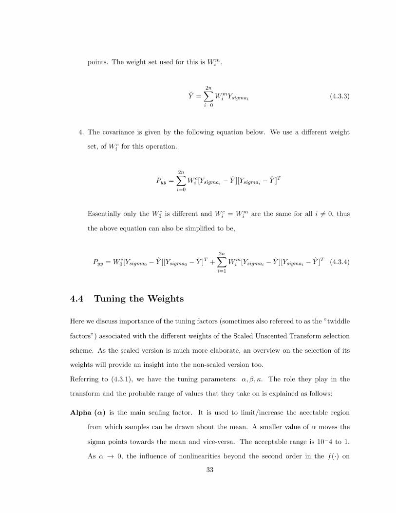
4.4 Tuning the Weights
Here we discuss importance of the tuning factors (sometimes also refereed to as the ”twiddle
factors”) associated with the different weights of the Scaled Unscented Transform selection
scheme. As the scaled version is much more elaborate, an overview on the selection of its
weights will provide an insight into the non-scaled version too.
Referring to (4.3.1), we have the tuning parameters: α, β, κ. The role they play in the
transform and the probable range of values that they take on is explained as follows:
Alpha (α) is the main scaling factor. It is used to limit/increase the accetable region
from which samples can be drawn about the mean. A smaller value of α moves the
sigma points towards the mean and vice-versa. The acceptable range is 10−4 to 1.
As α → 0, the influence of nonlinearities beyond the second order in the f(·) on
33

the approximated mean and covariance is theoretically reduced[6]. When α = 1, the
scaled unscented transform is the same as the normal unscented transform.
Beta (β) is used to incorporate prior knowledge of the distribution of x. For Gaussian
distributions we usually set it to 2 (optimal)[3].
Kappa (κ) is just a secondary scaling parameter. We usually set it to 0 for state estimation
[3]. When κ = 0 the Xsigma0 point is effectively omitted from the calculations of the
mean and covariance calculations. Putting a negative value in κ might affect the
positive semi-definiteness of the transformed covariance[6].
4.5 The UKF Algorithm
There are two versions of the Unscented Kalman Filter, the augmented and the non-
augmented. I illustrate the use of the non-scaled unscented transform in each of the filters
below for reasons of simplicity and ease of understanding the algorithm. Once, the cen-
tral theme of the UKF is grasped, one can use either the scaled or the unscaled transform
depending on what the application demands.
4.5.1 Augmented UKF
Its name is augmented because we need to augment the state vector to include the process
disturbance. Thus, the dimensionality of the augmented state vector xa becomes na = n+q
where q is dimension of the process disturbance variance Q. Thus,
xak =
xk
0qx1
34

we also include the process disturbance variance in our main error covariance matrix Pxx
augmenting it to,
P axxk =
Pxxk 0nxq
0qxn Q
Now, we begin the UKF:
1. The set of 2na + 1 Sigma Points are created by employing the selection scheme men-
tioned in (4.2.1) to the augmented state mean xakand covariance P axx
Xak0 = xak W0 =
κ
na + κ(4.5.1a)
Xaki
= xak +(√
(na + κ)P axxk
)i
Wi =1
2(na + κ)(4.5.1b)
Xaki+na = xak −
(√(na + κ)P axxk
)i
Wi+n =1
2(na + κ)(4.5.1c)
Here the Xaki
denotation is used for the sigma points, as writing ’sigma’ in each of
them would make it very cumbersome to read.
2. Pass each point through the nonlinear function f, to obtain the transformed sigma
points X(−)ak+1i
X(−)ak+1i= fa(Xa
ki, uk) (4.5.2)
3. The a priori, indicated by the minus(-) sign, mean x(−)ak+1 is given by
x(−)ak+1 =
2na∑i=0
WiX(−)ak+1i(4.5.3)
35

4. And the a priori covariance P (−)axxk+1is computed as,
P (−)axxk+1=
2na∑i=0
Wi[X(−)ak+1i− x(−)ak+1][X(−)ak+1i
− x(−)ak+1]T (4.5.4)
5. Pass all these transformed sigma points through the observer function h, to obtain
the Y sigma points Yk+1i
Yk+1i = h(X(−)ak+1i, uk) (4.5.5)
6. Compute the mean yk+1 and covariance Pyyk+1of these observer sigma points,
yk+1 =2na∑i=0
WiYk+1i (4.5.6a)
And since the observation noise is additive(especially in our case it is truly additive),
we can just add the measurement noise variance R to Pyyk+1to get the following,
Pyyk+1= R+
2na∑i=0
Wi[Yk+1i − yk+1][Yk+1i − yk+1]T (4.5.6b)
7. Calculate the Cross-Covariance between the X and Y sigma points
Pxy =2na∑i=0
Wi[X(−)ak+1i− x(−)ak+1][Yk+1i − yk+1]
T (4.5.7)
8. The measurement update part of the UKF is the same as that for the MCKF (see the
equations on page 25)
The Kalman Gain is given as,
Kk+1 =PxyPyyk+1
(4.5.8a)
36

The a posteriori mean is given as,
x(+)ak+1 = xa(−)k+1 +Kk+1[yk+1 − yk+1] (4.5.8b)
where yk+1 is the true measurement obtained at the k+ 1th step. Also, this is the end
of the filtering process block so need to extract the non-augmented state vector back
again, thus
x(+)k+1 = x(+)ak+1[1 : n]
And, Finally the a posteriori covariance is given as,
P (+)xxk+1= P (−)xxk+1
−Kk+1Pyyk+1KTk+1 (4.5.8c)
Note: The reason why we augment the state vector, is to incorporate the effects of the
process disturbance on the mean and covariance of the sigma points. This does mean
that we have more sigma points to propagate, but it also means that the effect of the
process disturbance are introduced with the same order of accuracy as the uncertainty in
the state. Such an augmented scheme also implies that correlated noise sources can be
implemented easily[2]. Also, one can extend this model in a similar fashion to incorporate
the measurement noise inn the mean and covariance, if it is non-additive or incorporated
in a nonlinear fashion in the observer (we do not do this since in our case for the mobile
robots, we assume additive white Gaussian measurement noise). Thus, the augmented
implementation is favoured when our process disturbance and/or measurement noise is
introduced into the system in a nonlinear and/or non-additive way. Plus, unlike the EKF
the UKF does not place any restrictions on the noise sources to be Gaussian RVs.
4.5.2 Non-augmented UKF
If we know that the process disturbance(and/or measurement noise) is additive in the state
propagation then we do not need to augment the state vector and thus can reduce the
dimensionality and number of our sigma points and save on some computational costs.
Since, not a lot is changed in the implementation, I will only outline the differences in the
non-augmented UKF algorithm instead of rewriting it.
37

1. The Selection scheme remains the same as described in (4.2.1), as we do not tamper
with xk, Pxxk or n.
2. Generate the sigma points and instantiate them through the nonlinear function f and
obtain the mean of the transformed sigma points. However, when we are calculat-
ing the covariance of the transformed sigma points we add the process disturbance
variance Q to it, altering (4.5.4) as follows,
P (−)xxk+1= Q+
2n∑i=0
Wi[X(−)k+1i − x(−)k+1][X(−)k+1i − x(−)k+1]T (4.5.9)
but because we just included the effects of the process disturbance in the error co-
variance, we need to redraw the sigma points again, to incorporate this effect in the
sigma points. We do this by using the recently obtained mean X(−)k+1 and covariance
P (−)xxk+1in the selection scheme given by (4.2.1).
3. The rest of the procedure remains the same as in (4.5.1)
4.6 The Square Root UKF
The drawback of the UKF is its computational complexity and comparatively slow speed
of operation (as to that of the EKF), thus despite its superior performance over the EKF
it still is not used in applications that are constrained by low computational capabilities.
Thus, if we could find a way to increase the computational efficiency of the UKF while still
maintaining its efficient filtering index, we will have on our hands an efficient and fast state
estimator and online filtering tool. The Square Root UKF does just this.
Rudolph Van der Merwe and Eric Wan introduced the Square-Root Unscented Kalman
Filter. The following reasoning and algorithm are taken from their paper on the same[3].
The most computationally expensive operation in the UKF corresponds to calculating the
new set of sigma points at each time update. While√Pxx is an integral part of the UKF, it is
38

still the full covariance Pxx which is recursively updated. In the SR-UKF implementation, S,
which is the square root of Pxx will be propagated directly, avoiding the need to refactorize
at each time step.
The Square Root form of the UKF use the following linear algebraic techniques:
Qr Decomposition The OR decomposition or factorization of a matrix Al∗n is given by
AT = QR, where Qn∗n is an orthogonal matrix and Rn∗l and n ≥ l. The upper right
triangular part of R, R, is the transpose of the Cholesky factor of P = AAT . This
culminates into R = ST . The notation used for the QR decomposition operation of a
matrix that just returns R is: ’qr{·}’2.
Cholesky Factor Updating If S is the original Cholesky factor of P = AAT , then the
Cholesky factor of the rank 1 update or downdate, P ±√vuuT is denoted as S =
cholupdate{S, u,±v}. If u is a matrix and not a vector, then we simply perform the
cholupdate{S, coli,±v} consecutively, for i = 1 : M where M is the number of columns
of the matrix u and coli denotes the ith column of u.
Efficient Least Squares The solution to the equation (AAT )x = AT b also corresponds
to the solution of the overdetermined least squares problem Ax = b. This can be
solved efficiently using a QR decomposition with pivoting (implemented in Matlab’s
’/’ operator).
Before we start the algorithm, a note on why we are using the Cholesky factorization /
decomposition method for the initial matrix square root:
If we have a positive semi-definite matrix P , then it can have many square roots. In addition
to this for any real valued matrix S that satisfies the following equation,
P = SST
2For further inquiry as to what is the exact computational complexity of the operations described in thesquare root UKF refer to the source[3]
39

is a valid square root of P . Now, one of the forms of the Cholesky Decomposition of a
matrix is,
A = RTR
where R is an upper triangular matrix. Thus, we can use the Cholesky Decomposition of
the covariance matrix as an alternative to its usual matrix square root. The advantage of
this being added numerical efficiency and stability as the Cholesky factors of P are generally
much better conditioned for matrix operations than P itself. The idea of using a Cholesky
factor for covariance matrix was first implemented by James E. Potter in his efforts to
improve the numerical stability of the measurement update equations. His implementation
came to be called as square-root filtering. 3.
4.6.1 The SR-UKF Filter Algorithm
1. Initialize with the initial estimate of the state vector to be X0 and the initial error
covariance to be P0. Thus, forming the Cholesky factor of P0,
S0 = cholP0
Also, the weight values need to assigned at this point.For this algorithm I employ the
scaled unscented transform scheme mentioned in 4.3.
2. We start with the cyclic process that is repeated at each iteration. The iteration being
marked by k and the sigma points being denoted by the lowercase i.
3More details on this can be found in the chapter ”Implementation Methods” in the book ”KalmanFiltering: Theory and Practice using Matlab”[6]
40

Generate the sigma points using the Cholesky factor of the error covariance S(+)k,
Xk0 = x(+)k (4.6.1a)
Xki = x(+)k + γSk for i = 1, 2, . . . , n (4.6.1b)
Xki+n= x(+)k + γSk for i = n+ 1, . . . , 2n (4.6.1c)
(4.6.1d)
3. Instantiate each sigma point through the nonlinear function f,
X(−)k+1i = f(Xki , uk) for i = 0, 1, . . . , 2n
4. Now forming the new mean and covariance of the transformed sigma points,
x(−)k+1 =2n∑i=0
Wmi X(−)k+1i (4.6.2a)
The a priori time-update of the Cholesky factory of the error covariance if formed
using the QR decomposition of the compound matrix containing the weighted sigma
points from i = 1 to i = 2n
S(−)k+1 = qr{[√W ci (X(−)k+1|i=1:2n − x(−)k+1)
√Q]} (4.6.2b)
Where the operation (X(−)k+1|i=1:2n−x(−)k+1) implies subtraction of the mean from
each of the sigma points.
A separate subsequent Cholesky update/downdate is necessary since the weight of the
0th sigma point W c0 maybe negative
S(−)k+1 = cholupdate{S(−)k+1, X(−)k+10 − x(−)k+1,Wc0} (4.6.2c)
41

5. Redraw the sigma points to incorporate the effect of the process disturnce in them,
since we are using the non-augmented version of the UKF.
6. Instantiate each point through the observer function h,
Yk+1i = h (X(−)k+1i , uk) for i = 0, 1, . . . , 2n
7. Find the mean and covariance of the now transformed Yk+ii sigma points in a similar
fashion
yk+1 =2n∑i=0
Wmi Yk+1i (4.6.3a)
SY :k+1 = qr{[√W ci (Yk+1|i=1:2n − yk+1)
√R]} (4.6.3b)
SY :k+1 = cholupdate{SY :k+1, Yk+10 − yk+1,Wc0} (4.6.3c)
8. Finding the Cross-Covariance of X and Y sigma points and the Kalman Gain,
Pxy =2n∑i=0
W ci [X(−)k+1i − x(−)k+1][Yk+1i − yk+1]
T (4.6.4a)
Since the SY :k+1 is a square and triangular matrix, efficient ”back-substitutions” can
be used to solve for the Kalman gain Kk+1 directly without the need for a matrix
inversion,
Kk + 1 = (Pxy/STY :k+1)/SY :k+1 (4.6.4b)
9. Finally, after getting the actual sensor measurements for the k + 1th step, yk+1, we
make the a posteriori updates to the mean and the Cholesky factor of the error
covariance,
x(+)k+1 = x(−)k+1 +Kk+1(yk+1 − yk+1) (4.6.5a)
42

The a posterior measurement update of the Cholesky factor of the state covariance
is calculated by applying m sequential Cholesky downdates to S(−)k+1, where m is
the number of columns of the matrix Kk+1SY :k+1, and the downdate vectors are the
columns of this matrix.
S(+)k+1 = cholupdate{S(−)k+1,Kk+1SY :k+1,−1} (4.6.5b)
Out of all the UKF implementation versions, the square-root UKF has better numeri-
cal properties and guarantees positive semi-definiteness of the underlying state covariance
Pxx[3].
4.7 An Illustrative comparison of the UKF with the EKF
Now, that we learnt about the various flavours of the UKF, let us examine an illustration
comparing estimation accuracy of the EKF and the UKF for the mean and error covariance
of the state vector x, after it is transformed through a nonlinear function. To better gauge
the performance of either of these filters, we juxtapose them with a Monte-Carlo Sampling
Method(with a large number of samples), which can be taken as the ground value for the
’true’ mean and error covariance of the state.
43

Figure 4.2: Comparison of mean and covariance sampling by Monte-Carlo Sampling, EKFand UKF[3]
44

Chapter 5: Results: Simulation and Analysis
5.1 Matlab Simulation
Matlab is used for simulating my system and filter design. The reasons for choosing Matlab
are:
1. Controls and Electrical engineering community favours it. Hence, many will find it
easy to read and analyze my code, thereby relating to it.
2. Prototyping is very easy on Matlab. Thus one can concentrate more on the filter
design rather than worry about its implementation.
3. It provides in-built support for Matrix Operations. The Kalman Filter relies heavily
on Matrix Math, thus, it makes Matlab a convenient environment.
4. Excellent Plotting and Graphing support.
Matlab does have certain inefficiencies which makes it very slow when compared to other
programming languages like C,C++,etc. However, all the filters are written in Matlab,
thus evaluating them is still based on a fair comparison. One can switch to a C/C++
implementation when dealing with a real-time implementation of the Filter for a truly
efficient and fast operation.
The codes used for the simulations and other verification schemes can be used to recreate
any of the results and plots documented in the sections below. The codes are attached in
the appendix section (on page A) and for further help with them you can contact me at
45
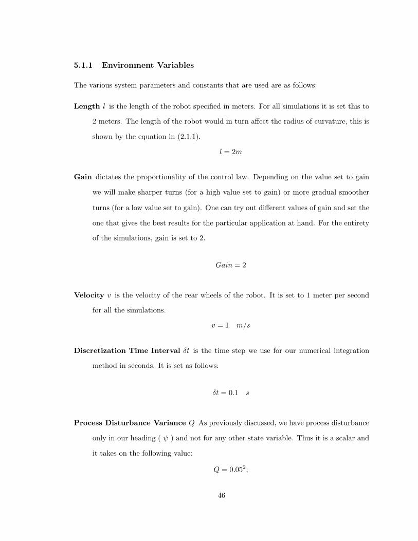
5.1.1 Environment Variables
The various system parameters and constants that are used are as follows:
Length l is the length of the robot specified in meters. For all simulations it is set this to
2 meters. The length of the robot would in turn affect the radius of curvature, this is
shown by the equation in (2.1.1).
l = 2m
Gain dictates the proportionality of the control law. Depending on the value set to gain
we will make sharper turns (for a high value set to gain) or more gradual smoother
turns (for a low value set to gain). One can try out different values of gain and set the
one that gives the best results for the particular application at hand. For the entirety
of the simulations, gain is set to 2.
Gain = 2
Velocity v is the velocity of the rear wheels of the robot. It is set to 1 meter per second
for all the simulations.
v = 1 m/s
Discretization Time Interval δt is the time step we use for our numerical integration
method in seconds. It is set as follows:
δt = 0.1 s
Process Disturbance Variance Q As previously discussed, we have process disturbance
only in our heading ( ψ ) and not for any other state variable. Thus it is a scalar and
it takes on the following value:
Q = 0.052;
46

Measurement Noise R is the variance of the measurement noise. For all the filters, I
include measurement noise only in the x and y coordinate. It is absent from the ψ
variable as ψ is not measured at all. The value of the R matrix is given below:
R =
0.22 0
0 0.22
Initial Error Covariance P0 is the value given by E[(X0 −X0)(X0 −X0)T ]. Here X0 is
the initial best guess of the state vector before beginning with the filtering operation.
X0 is the true state vector (used for our simulations). Since we neither have knowledge
of the PDF of the state vector X nor access to the true state vector X0, we set this
value arbitrarily. Trial and error methods are used to fine tune this value to increase
the accuracy of the filter. The value used in all the simulations is given as:
P0 =
0.22 0 0
0 0.22 0
0 0 ( π4.0)2
A note about the Initial Estimate of the state vector X0: This can be set to a completely
random value and allow the filter catch up to the true state at the expense of a certain
number of iterations of the simulation. Some approaches even assume that they have exact
knowledge of the initial conditions of the state, and set X0 = X0 and thus making P0 = 0nxn.
The approach used in this thesis sets X0 to a value near the true state (by including some
random noise over the value of the true state vector).
47

5.2 Graphs
Each of the filters are tested out on two different paths.
Path 1 The first path is more straightforward and has a single destination in its entire
course. However I make the observer function ( h(·) ) non-linear in the simulation for
this path. This is done on purpose to facilitate a comparison of the all the filters with
the IEKF, as the IEKF is only advantageous in the case of non-linearity in h(·).
The h(·) I employ is specifically this:
Y =
(xco−ord + noise)3
(yco−ord + noise)3
Since there are high non-linearities in this simulation, please consider the resultant
path plots and accuracy measures accordingly. There is a lot of noise present in them,
hence the skewed plots.
Path 2 The second path has a linear h(·), but, it has multiple destination (analogous to
checkpoints) fed to it in a sequential manner. It first completes the entire path to the
first checkpoint in the list and then once it has reached that destination (with a small
room for error) it removes that checkpoint from the list and moves on to the next set
of destination coordinates. The list of the destination coordinates is provided in the
following manner:
Xdes =
xdes1 xdes2 . . . xdesp
ydes1 ydes2 . . . ydesp
Here, p is the total number checkpoints in the list.
Note: The flavour of UKF used in the simulations and comparisons that are documented
below is the Scaled Unscented Kalman Filter (non-augmented).
48

5.2.1 EKF Path 1
−8 −6 −4 −2 0 2 4 6 8 10−2
0
2
4
6
8
10Robot Trajectory in X−Y Space
X−Axis
Y−
Axi
s
True StateEstimated State
Figure 5.1: EKF Plot for True v/s Estimated Robot Trajectory
0 50 100 150 200 250 300−4
−3
−2
−1
0
1
2
3Plot of Robot Heading Angle(psi)
Time (Iteration Number)
Hea
ding
Ang
le (
psi)
True StateEstimated State
Figure 5.2: EKF Plot for True v/s Estimated Heading Angle
49

5.2.2 EKF Path 2
−4 −2 0 2 4 6 8 100
2
4
6
8
10
12
14Robot Trajectory in X−Y Space
X−Axis
Y−
Axi
s
True StateEstimated State
Figure 5.3: EKF Plot for True v/s Estimated Robot Trajectory
0 50 100 150 200 250 300 350 400 450−4
−3
−2
−1
0
1
2
3
4Plot of Robot Heading Angle(psi)
Time (Iteration Number)
Hea
ding
Ang
le (
psi)
True StateEstimated State
Figure 5.4: EKF Plot for True v/s Estimated heading Angle
50

5.2.3 IEKF Path 1
−6 −4 −2 0 2 4 6 8 10 12−2
0
2
4
6
8
10
12
X−Axis
Y−
Axi
s
True StateEstimated State
Figure 5.5: IEKF Plot for True v/s Estimated Robot Trajectory
0 50 100 150 200 250 300−3
−2
−1
0
1
2
3
4Plot of Robot Heading Angle(psi)
Time (Iteration Number)
Hea
ding
Ang
le (
psi)
True StateEstimated State
Figure 5.6: IEKF Plot for True v/s Estimated Heading Angle
51

5.2.4 IEKF Path 2
−4 −2 0 2 4 6 8 100
2
4
6
8
10
12
14
X−Axis
Y−
Axi
s
True StateEstimated State
Figure 5.7: IEKF Plot for True v/s Estimated Robot Trajectory
0 50 100 150 200 250 300 350 400 450−4
−3
−2
−1
0
1
2
3
4Plot of Robot Heading Angle(psi)
Time (Iteration Number)
Hea
ding
Ang
le (
psi)
True StateEstimated State
Figure 5.8: IEKF Plot for True v/s Estimated heading Angle
52

5.2.5 UKF Path 1
−6 −4 −2 0 2 4 6 8 10 12−2
0
2
4
6
8
10
12Robot Trajectory in X−Y Space
X−Axis
Y−
Axi
s
True StateEstimated State
Figure 5.9: UKF Plot for True v/s Estimated Robot Trajectory
0 50 100 150 200 250 300−4
−3
−2
−1
0
1
2
3
4Plot of Robot Heading Angle(psi)
Time (Iteration Number)
Hea
ding
Ang
le (
psi)
True StateEstimated State
Figure 5.10: UKF Plot for True v/s Estimated Heading Angle
53

5.2.6 UKF Path 2
−4 −2 0 2 4 6 8 100
2
4
6
8
10
12
14Robot Trajectory in X−Y Space
X−Axis
Y−
Axi
s
True StateEstimated State
Figure 5.11: UKF Plot for True v/s Estimated Robot Trajectory
0 50 100 150 200 250 300 350 400 450−4
−3
−2
−1
0
1
2
3
4Plot of Robot Heading Angle(psi)
Time (Iteration Number)
Hea
ding
Ang
le (
psi)
True StateEstimated State
Figure 5.12: UKF Plot for True v/s Estimated heading Angle
54

5.2.7 Accuracy and Computational Costs (Time)
The accuracy of the filters is measured by calculating their Mean Squared Error (MSE)
over the entire length of the simulation. Note that the MSE for x and y coordinates is
calculated together and that of the ψ is calculated separately as they have different units
of measurement (meters and radians respectively).
Functions are made to carry out specific subroutines. This approach makes it possible to
measure the time spent in each function and compare it for the various different filters.
Matlab’s ’Run and Time’ feature enables this and gives the necessary numbers to facilitate
a comparison between filters.
A list of the various functions used and their descriptions:
stateprop this is where the system dynamics of the mobile robot are coded. The only
function of stateprop is to propagate the state forward by 1 time step as per the
specified dynamics.
anglenormalization serves the function of keeping the angle values in the range of 0 to
π. If this is not done regularly at every iteration and major alteration to the angles,
it might lead to a very unstable performance of the filter.
The tables below gives us a comparison of the filters with respect to accuracy and speed.
The stateprop and anglenorm represent the time spent in those functions respectively. All
time is in seconds.
Table 5.1: Comparison Table for Path 1
Filters MSE (x and y) MSE ψ Total Time stateprop anglenorm
EKF 0.5188 0.8391 0.183 0.008 0.017
IEKF 0.4206 0.8726 0.560 0.026 0.009
UKF 0.5001 0.7616 1.527 0.157 0.039
55

Table 5.2: Comparison Table for Path 2
Filters MSE (x and y) MSE ψ Total Time stateprop anglenorm
EKF 0.0069 0.0063 0.225 0.009 0.009
IEKF 0.0069 0.0063 1.786 0.083 0.093
UKF 0.0063 0.0064 2.657 0.255 0.036
5.3 Verification of the UKF Implementation
Such below average performance of the UKF leads to questioning weather its implementation
scheme is correct or not. This combined with the fact that every one in the Controls Industry
believes that the UKF is superior to the EKF, led to the development of verification schemes
for the UKF.
5.3.1 Testing the Unscented Transform
The Unscented Transform is at the heart of the UKF. The rest is just the filtering algorithm,
where the possibility of error is thin. Thus, if we check the functioning of the Unscented
Transform to be correct and as desired, we can actually state with authority that indeed for
this specific case of Mobile Robot State Estimation it is better to stick to the EKF. There
are basically two aspects that need to be verified with the Unscented Transform:
Proper Selection of the Sigma Points
The Sigma points chosen in the UKF (or any filter from the family of Sigma Point Kalman
Filters) are chosen deterministically. This poses the question that on a meta-level: What is
the underlying scheme for selecting the sigma points in the Unscented Transform? Investi-
gating this would also provide a much better understanding of the transform.
The sigma points are chosen along the principal axis of the ellipse of the uncertainty covari-
ance. Since in our case the system dynamics are 3-dimensional the uncertainty covariance
i.e. Pxx translates to an ellipsoid. So to really confirm if our sigma points are truly being
mapped along the principal axis of this ellipsoid we need to first draw this ellipsoid.
56

Now, to grasp the concept of this ellipsoid we need to consider another fact. There is a
confidence region boundary that we need to stick inside. This is because we assume our
State Vector Random Variable to be Gaussian in nature, and as such the Gaussian region
of convergence spreads till infinity. Thus as a practical measure we restrict this boundary
to include ’almost all’ area under the ellipsoid but not all, since as we progress further and
further away from the mean the probability of the state vector residing in that space reduces
drastically. For the particular verification scheme being implemented, the confidence region
is set to 65%1.
The following steps are based off the work done in the following articles[12] [13].
1. Scale covariance matrix (Pxx) with the Mahalanobis Distance. The Mahalanobis
distance is given by the following Matlab command:
mahalanobis distance = chi2inv(conf, dim);
where ’conf’ is the confidence region as mentioned above and ’dim’ is the dimension
of the state vector (which in our case is 3).
2. Obtain the Eigen Values and Eigen Vectors of the Covariance Matrix
[V,D] = eig(P);
% Make sure that all our eigen values and vectors are real & non−negative
V = real(V);
D= real(D);
D = abs(D);
% Sorting the Eigen vectors by their eignevalues in a decending order
[D order] = sort(diag(D), 'descend');
D = diag(D);
V = V(:, order);
1This value was attained empirically
57

3. Generate the points for a generic sphere
[X,Y,Z] = sphere(num);
4. Now we conform these generated sphere points to the surface of our Ellipsoid
L= sqrt(diag(D));
w = (V*sqrt(D))* [X(:)'; Y(:)'; Z(:)'];
z = repmat(Mu(:), [1 (num + 1)ˆ2]) + w;
here ’Mu’ is the mean of our State Vector (X) around which the ellipsoid is centered.
5. Now just plot these generated points
holding = ishold;
axis equal
rotate3d on;
shading flat
s = mesh(reshape(z(1, :), [(num + 1) (num + 1)]), ...
reshape(z(2, :), [(num + 1) (num + 1)]), ...
reshape(z(3, :), [(num + 1) (num + 1)]));
set(s,'EdgeColor',[0,0,0],'EdgeAlpha',0.05,'FaceColor','none');
% The line below allows me to exclude the sphere itself from the legend
set(get(get(s,'Annotation'),'LegendInformation'),'IconDisplayStyle','off');
6. Plotting the Principal Axis of the Ellipsoid
% First the x−axis
h = plot3([Mu(1); Mu(1) + L(1) * V(1, 1); Mu(1) − L(1) * V(1, 1)], ...
[Mu(2); Mu(2) + L(1) * V(2, 1); Mu(2) − L(1) * V(2, 1)], ...
[Mu(3); Mu(3) + L(1) * V(3, 1); Mu(3) − L(1) * V(3, 1)], ...
'Color','blue');
58

% Now the y−axis
h=[h;plot3([Mu(1); Mu(1) + L(2) * V(1, 2); Mu(1) − L(2) * V(1, 2)], ...
[Mu(2); Mu(2) + L(2) * V(2, 2); Mu(2) − L(2) * V(2, 2)], ...
[Mu(3); Mu(3) + L(2) * V(3, 2); Mu(3) − L(2) * V(3, 2)], ...
'Color','black')];
% And finally the si−axis (this is the z−axis)
h = [h; plot3([Mu(1); Mu(1) + L(3) * V(1, 3); Mu(1) − L(3) * V(1, 3)], ...
[Mu(2); Mu(2) + L(3) * V(2, 3); Mu(2) − L(3) * V(2, 3)], ...
[Mu(3); Mu(3) + L(3) * V(3, 3); Mu(3) − L(3) * V(3, 3)], ...
'Color','red')];
With this done we can now plot an instance of the generated sigma points to check if they
truly lie on the Principal Axes.
The first plot is done with the value of α = 0.5, as discussed in (4.3.1) α is the spread of
the sigma points about the mean.
Figure 5.13: Error Covariance Ellipsoid: Sigma points around the mean with α = 0.5
59

As we can infer from the above figure 5.13, the spread of the sigma points about the mean
is symmetric. There are two equidistant sigma points on either side of the mean on each
of the principal axes of the ellipsoid. The distance of these sigma points from the mean is
the same for all the 2 ∗ n+ 1 points (where n is the dimension of the state vector). As for
verifying the proper functioning of alpha, we can tweak it around a bit and plot the spread
again. The figure below shows the sigma points on the error ellipsoid when2 α = 0.9.
Figure 5.14: Error Covariance Ellipsoid: Sigma points around the mean with α = 0.9
Thus, we can now conclude without a doubt that the sigma point selection scheme is working
as intended.
2The larger the vallue of α the farther away from the mean the sigma points will spread.
60

Testing the Convergence of the Unscented Transform
The Unscented Transform (or Scaled Unscented Transform) should be convergent for our
filter to maintain stability and not loose track of the state being estimated. There exists a
very simple scheme to perform this verification. It is as follows:
1. With the initial Data given (i.e. Pxx, α, β, γ,Wm&W c and the mean X) generate set
of sigma points as per the equations in (4.3.2).
2. We then pass these points through an identity transform, which basically means we
do not touch these points at all.
3. Next we generate the mean and covariance of the transformed sigma points as de-
scribed in (4.3.3) and (4.3.4) respectively.
4. Since we passed our sigma points through an identity transform, the state of the
system should remain the same. Thus, the mean and covariance generated in the step
above should match with the ones we started off with in the first place. If this does
not hold then the Unscented Transform will be divergent and all will fail.
A code snippet was written in Matlab for executing this verification scheme. Before the
identity transform the mean and covariance were:
Pplus =
0.0400 0 0
0 0.0400 0
0 0 0.6169
Xest =
0.1212
0.1081
1.2818
And after the identity transform the calculated statistics were:
61

Xest ident =
0.1212
0.1081
1.2818
Pminus ident =
0.0400 0.0000 −0.0000
0.0000 0.0400 −0.0000
−0.0000 −0.0000 0.6169
As one can see the mean remains unaltered. As for the covariance, the misplaced − signs
arise due to round-off and other computational errors. But these too are after the fourth
decimal place, thus it is safe to conclude that are transform is actually convergent and
working properly.
5.4 Averaging over multiple runs
One possible explanation to the current scenario of results would be the random noise
induced into the system via process disturbance and measurement noise. Since these vary
from run to run3 it is always considered a good practice to average any Meas Square
Error(MSE) over a good number of runs so that we eliminate the dependence of the results
on randomness.
For the case at hand, we will compare just the EKF and the scaled UKF (non-augmented)
over a thousand runs as this would allow us a more in-depth analysis of what the true MSE
of each of them in the long run might be. To play it safe, the MSEs of each of the filters
were averaged over 1000 different runs (which means thousand different sets of random noise
values). Path 2, as mentioned in the Graphs section above (Sec. 5.2), was used for these
runs. The results obtained are shown in the table below.
3They were still the same sets used to compare the filters in the sections above
62

Table 5.3: EKF v/s UKF MSE averaged over 1000 runs
Filter MSE (x and y) MSE ψ
EKF 0.0038 0.0412
UKF 0.0039 0.0400
5.5 Inference
The current claim in the Controls Community is that the UKF outperforms the EKF for
non-linear applications and does just as well for linear applications. While this is true for
the various non-linear systems that the UKF has been applied to, the results specific to the
case of Mobile Robot State Estimation are quite the contrary. This might be a case of the
peculiar system dynamics of the Mobile Robot which causes this.
Thus, the most effective method for Mobile Robot State Estimation still remains to be the
Extended Kalman Filter. In cases, when the noise level is too high the Iterated Extended
Kalman Filter should be employed if the computational costs can be entertained.
The final conclusive finding of my comparison would be that the Extended Kalman Filter,
is by far the best method for Mobile Robot State Estimation, within the realm of Gaussian
Filters. Even outside the field of Gaussian Filters it is still the alternative with the highest
accuracy to computational cost ratio.
5.6 Future Scope
The following are some extensions that could be built upon the work and analysis done in
this thesis:
• Theoretical Investigation of why the UKF performs below par for the Mobile Robot
problem.
• A mathematical proof of concept as to why the UKF does not give higher accuracy
than the EKF for the Mobile Robot State Estimation.
• A possible change to UKF tailored for the current system dynamics filtering.
63

Appendix A: Matlab Codes
All the codes that are included here are to be placed in the same directory for them to work
properly. These include some Matlab function files which are used in a number of different
codes of the respective filters. The actual codes are outlined a box with the title of the
filter or function it is on top (outside the box). The descriptions of the functions used were
mentioned in the following section 5.2.7.
Angle Normalization Function
function [ang] = angle normalization(ang)
% angle normalization Normalizes Angles to be in the range of 0 to pi
% It subtracts 2*pi if the value of ang is greater than pi, and, it adds
% 2*pi if the value of ang is less than −pi. If it is already in the
% range of [0,pi] then it just returns the value of ang as is.
if ang > pi
ang = ang − 2*pi;
end
if ang < −pi
ang = ang + 2*pi;
end
State Propagation Function
function [Xcur] = stateprop(Xcur,u,t,v)
% State Forward Propagation Function
% This is where the actual system dynamics equations of the function are
% used. The function takes the current state 'Xcur' as well as
% the control input generated 'u' at current time instant and generates
64

% the forward propagated State Vector update in 'Xcur' itself and ...
returns it.
% You need to provide the discretization time step 't' to this function.
%
% 'v' is the velocity of the rear wheels of the robot in meters/s
%
% These parameters are relative to the system your using and will change
% accordingly.
%
% When using this function for simulating the true state, the standard
% deviation of the process disturbance matrix(or vector/single value) ...
'std'
% must be included in u and then passed to the function. (in whichever
% way i.e. addtive/non−additive it should already be incorporated within
% u when u is provided to "stateprop")
%s
% This function is particularly coded for my specific set of araangements
% of the mobile robot state dynamics and choice of process disturbance.
% If you wish to use my code for tour own purposes make sure to change
% this code to the appropriate version as desired by your state
% propagation dynamics!
Xcur = Xcur + t*[−v*sin(Xcur(3)) v*cos(Xcur(3)) u]';
end
Extended Kalman Filter for the Mobile Robot
%function [error sum si error] = mobile robot ekf()
clear all;
65

close all;
clc;
%rng default; % This is to reset Matlab Random Number Generators seed to the
% same value everytime so that we can use it
%% Specifying and defining various constants and control parameters
R1=0.2ˆ2;
Q=0.05ˆ2;
sR1 = sqrt(R1);
sQ = sqrt(Q); % Square root of Q (as Q does not change in my case, it is
% computationaly cheaper to precompute its sqrt and keep, instead of
% computing it at every step of the simulation)
t=0.1; % Sample Time Interval in seconds (i.e this is delta t)
l=2.0; %Length of the Robot in meteres
v=1.0; % Velocity of rear wheels
vlr = v/l; % I precompute the ratio of v/l so as to not perform this divison
% every iteration of the simulation thereby cutting on some computational
% costs
gain=2; %Sterring gain specified
%% Specifying the Initial Conditions
% Set of Destination Co−ordinates [xdes1 ydes1;xdes2 ydes2;...]'
% Xdes=[5 0;5 5;10 10]';
% Xdes = [10 10]'; % Path I
%Xdes = [−4 4;0 8;4 4;0 0]'; % Trace of a Rhombus
Xdes=[0 4;0 8;0 12;9 9;4 4;0 0]'; % Curvy Path −− Path II
X=[0 0 pi/2]'; %Initial Co−ordintes at start (also the true State Vector ...
as [x y head]')
gain=2; %Sterring gain specified
66

%% Initial Estimation Parameters
Xest=X + sqrt(R1)*[randn randn randn]'; %Initial 0 state
R = [R1 0;0 R1];
Pminus=[R1 0 0;0 R1 0;0 0 (pi/4.0)ˆ2];
Pplus=Pminus;
H=[1 0 0;0 1 0]; % Since only x and y are measured and not heading
error sum = 0; % Initialize the summing up var. for MSE in the (x,y) coords
si error sum = 0; % Do the same for si (as si is measured in rads it cannot
% be combined with x and y cordinates)
%% The following variables are for specifying trajectory control and so on.
counter = 1; % Counter for the waypoints along the trajectory at which the
% Xdes point changes
cntlen=size(Xdes);
cntlen=cntlen(2);
tmpflag=0;
%% Now our online estimation loop begins.
% Here we simulate the true state of the System as well as seperately
% estimate using the EKF.
for i=1:1200
tmpflag = tmpflag +1;
if (((Xdes(:,counter) − Xest(1:2,i))'*(Xdes(:,counter) − ...
Xest(1:2,i)) < 0.1) && tmpflag >5)
if counter == cntlen
break;
end
tmpflag = 0;
counter=counter+1;
67

end
hdes= −atan2(Xdes(1,counter)−Xest(1,i),Xdes(2,counter)−Xest(2,i)); ...
%Desired Heading Angle
headest=Xest(3,i);
% Correcting angles and calculating alpha
hdes = angle normalization(hdes);
tmp=angle normalization(hdes−headest);
% The if−else case below places a limit on the maximum value of alpha
% to be pi/4.
if abs(gain*tmp)<=pi/4.0
alpha=gain*tmp;
else
alpha=pi*sign(tmp)/4.0;
end
% Simulating the true state of the robot
X(:,i+1) = stateprop(X(:,i),vlr*tan(alpha+sQ*randn),t,v); % ...
Propagating the State
% Normalize the angle for numerical safety and stability
X(3,i+1) = angle normalization(X(3,i+1));
% Extended Kalman Filter Prediction Steps
A=eye(3) + [0 0 −v*cos(headest); 0 0 −v*sin(headest);0 0 0]*t; % ...
Jacobian of the F Matrix
G=[0 0 v/(l*(cos(alpha))ˆ2)]'*t;
% Xest(:,i+1) = Xest(:,i) + t*[−v*sin(headest) v*cos(headest) ...
vlr*tan(alpha)]'; %This is actually the Xest(−) step
68

Xest(:,i+1) = stateprop(Xest(:,i),vlr*tan(alpha),t,v); %This is ...
actually the Xest(−) step
Pminus(:,:,i+1)= A*Pplus(:,:,i)*A' + G*Q*G'; % Error Covariance ...
Propagation(pre)
% Now we get the sensor Readings
Y=[X(1,i+1) X(2,i+1)]' + sR1*[randn randn]'; % Since only x and y ...
co−ords are measured
% The following code is for non−linear H−function comment it for ...
Path 2
% Y=Y.ˆ3;
% H=[3*Xest(1,i+1)ˆ2 0 0;0 3*Xest(2,i+1)ˆ2 0];
% This is where the non−linear code snippet ends and comment till here
% to remove the non−linearily in the H funciton
K=Pminus(:,:,i+1)*H'*inv(H*Pminus(:,:,i+1)*H' + R); %Kalman Gain
Xest(:,i+1) = Xest(:,i+1) + K*(Y−Xest(1:2,i+1)); % Adding the ...
Innovation!
Pplus(:,:,i+1)=[eye(3) − K*H]*Pminus(:,:,i+1)*[eye(3) − K*H]' + ...
K*R*K'; % Jospeh Form of the Post−Measurement Error Covariance ...
Belief
% Pplus(:,:,i+1) = [eye(3) − K*H]*Pminus(:,:,i+1);
% Correcting headest angle
Xest(3,i+1) = angle normalization(Xest(3,i+1));
error sum = error sum + (Xest(1:2,i+1) − X(1:2,i+1))'*(Xest(1:2,i+1) ...
− X(1:2,i+1));
69

si error sum = si error sum + (Xest(3,i+1) − X(3,i+1))'*(Xest(3,i+1) ...
− X(3,i+1));
end
error sum = error sum/i
si error = si error sum/i
figure;
hold on
grid on
plot(squeeze(X(1,:)),squeeze(X(2,:)),'r');
plot(squeeze(Xest(1,:)),squeeze(Xest(2,:)),'b');
title('Robot Trajectory in X−Y Space')
legend('True State','Estimated State')
xlabel('X−Axis')
ylabel('Y−Axis')
figure;
hold on
grid on
plot(squeeze(X(3,:)),'r')
plot(squeeze(Xest(3,:)),'b')
title('Plot of Robot Heading Angle(psi)')
xlabel('Time (Iteration Number)')
ylabel('Heading Angle (psi)')
legend('True State','Estimated State')
%end
Iterated Extended Kalman Filter for the Mobile Robot
clear all;
close all;
70

clc;
rng default; % This is to reset Matlab Random Number Generators seed to the
% same value everytime so that we can use it
%% Specifying and defining various constants and control parameters
R1=0.2ˆ2;
Q=0.05ˆ2;
sR1 = sqrt(R1);
sQ = sqrt(Q); % Square root of Q (as Q does not change in my case, it is
% computationaly cheaper to precompute its sqrt and keep, instead of
% computing it at every step of the simulation)
t=0.1; % Sample Time Interval in seconds (i.e this is delta t)
l=2.0; %Length of the Robot in meteres
v=1.0; % Velocity of rear wheels
vlr = v/l; % I precompute the ratio of v/l so as to not perform this divison
% every iteration of the simulation thereby cutting on some computational
% costs
gain=2; %Sterring gain specified
%% Specifying the Initial Conditions
% Set of Destination Co−ordinates [xdes1 ydes1;xdes2 ydes2;...]'
%Xdes=[5 0;5 5;10 10]';
Xdes = [10 10]'; % Path I
%Xdes = [−4 4;0 8;4 4;0 0]'; % Trace of a Rhombus
% Xdes=[0 4;0 8;0 12;9 9;4 4;0 0]'; % Curvy Path −− Path II
X=[0 0 pi/2]'; %Initial Co−ordintes at start (also the true State Vector ...
as [x y head]')
gain=2; %Sterring gain specified
71

%% Initial Estimation Parameters
Xest=X + sqrt(R1)*[randn randn randn]'; %Initial 0 state
R = [R1 0;0 R1];
Pminus=[R1 0 0;0 R1 0;0 0 (pi/4.0)ˆ2];
Pplus=Pminus;
H=[1 0 0;0 1 0]; % Since only x and y are measured and not heading
error sum = 0; % Initialize the summing up var. for MSE in the (x,y) coords
si error sum = 0; % Do the same for si (as si is measured in rads it cannot
% be combined with x and y cordinates)
%% The following variables are for specifying trajectory control and so on.
counter = 1; % Counter for the waypoints along the trajectory at which the
% Xdes point changes
cntlen=size(Xdes);
cntlen=cntlen(2);
tmpflag=0;
%% Now our online estimation loop begins.
% Here we simulate the true state of the System as well as seperately
% estimate using the IEKF.
cnt=[];
for i=1:1200
tmpflag = tmpflag +1;
if (((Xdes(:,counter) − Xest(1:2,i))'*(Xdes(:,counter) − ...
Xest(1:2,i)) < 0.1) && tmpflag >5)
if counter == cntlen
break;
end
tmpflag = 0;
72

counter=counter+1;
end
hdes= −atan2(Xdes(1,counter)−Xest(1,i),Xdes(2,counter)−Xest(2,i)); ...
%Desired Heading Angle
headest=Xest(3,i);
% Correcting angles and calculating alpha
hdes = angle normalization(hdes);
tmp=angle normalization(hdes−headest);
% The if−else case below places a limit on the maximum value of alpha
% to be pi/4.
if abs(gain*tmp)<=pi/4.0
alpha=gain*tmp;
else
alpha=pi*sign(tmp)/4.0;
end
% Simulating the true state of the robot
X(:,i+1) = stateprop(X(:,i),vlr*tan(alpha+sQ*randn),t,v); % ...
Propagating the State
% Normalize the angle for numerical safety and stability
X(3,i+1) = angle normalization(X(3,i+1));
% Extended Kalman Filter Prediction Steps
A=eye(3) + [0 0 −v*cos(headest); 0 0 −v*sin(headest);0 0 0]*t; % ...
Jacobian of the F Matrix
G=[0 0 v/(l*(cos(alpha))ˆ2)]'*t;
73

%Xest(:,i+1) = Xest(:,i) + t*[−v*sin(headest) v*cos(headest) ...
v*tan(alpha)/l]'; %This is actually the Xest(−) step
Xest(:,i+1) = stateprop(Xest(:,i),vlr*tan(alpha),t,v); %This is ...
actually the Xest(−) step
Pminus(:,:,i+1)= A*Pplus(:,:,i)*A' + G*Q*G'; % Error Covariance ...
Propagation(pre)
Xpriori=Xest(:,i+1);
% Now we get the sensor Readings
Y=[X(1,i+1) X(2,i+1)]' +sR1*[randn randn]'; % Since only x and y ...
co−ords are measured
Y=Y.ˆ3;
H=[3*Xest(1,i+1)ˆ2 0 0;0 3*Xest(2,i+1)ˆ2 0];
K=Pminus(:,:,i+1)*H'*inv(H*Pminus(:,:,i+1)*H' + R); %Kalman Gain
Xest(:,i+1) = Xest(:,i+1) + K*(Y − Xest(1:2,i+1).ˆ3); % This is ...
the Xest(:,I=1) (+) posterior form the EKF
% Now the IEKF begins its work by taking the Posterior provided by the
% EKF −−−−−−− The IEKF Part begins
Xlast=[0 0 0]';
Xcur=Xest(:,i+1);
eps=10;
k=0;
while eps > 1e−10
H=[3*Xcur(1)ˆ2 0 0;0 3*Xcur(2)ˆ2 0]; % Jacobian of the H Matrix
K=Pminus(:,:,i+1)*H'*inv(H*Pminus(:,:,i+1)*H' + R); %Kalman Gain
Ye = Y − [Xcur(1)ˆ3 Xcur(2)ˆ3]';
Xlast=Xcur;
Xcur = Xpriori + K*(Ye−H*(Xpriori − Xcur));
74

eps=norm(Xcur−Xlast,2);
%eps=(Xcur−Xlast)'*(Xcur−Xlast);
k=k+1;
end
cnt(i)=k;
Xest(:,i+1)=Xcur;
Pplus(:,:,i+1)=[eye(3) − K*H]*Pminus(:,:,i+1)*[eye(3) − K*H]' + ...
K*R*K'; % Jospeh Form of the Post−Measurement Error Covariance ...
Belief
% Correcting headest angle
Xest(3,i+1) = angle normalization(Xest(3,i+1));
error sum = error sum + (Xest(1:2,i+1) − X(1:2,i+1))'*(Xest(1:2,i+1) ...
− X(1:2,i+1));
si error sum = si error sum + (Xest(3,i+1) − X(3,i+1))'*(Xest(3,i+1) ...
− X(3,i+1));
end
error sum = error sum/i
si error = si error sum/i
figure;
hold on;
grid on;
plot(squeeze(X(1,:)),squeeze(X(2,:)),'r');
plot(squeeze(Xest(1,:)),squeeze(Xest(2,:)),'b');
legend('True State','Estimated State')
xlabel('X−Axis')
ylabel('Y−Axis')
75

figure;
hold on
grid on
plot(squeeze(X(3,:)),'r')
plot(squeeze(Xest(3,:)),'b')
title('Plot of Robot Heading Angle(psi)')
xlabel('Time (Iteration Number)')
ylabel('Heading Angle (psi)')
legend('True State','Estimated State')
figure;
hold on;
grid on;
plot(cnt);
Scaled Unscented Kalman Filter for the Mobile Robot
%function [error sum si error] = ukf sample mod scaled()
clear all;
close all;
clc;
rng default; % This is to reset Matlab Random Number Generators seed to the
% same value everytime so that we can use it
%% Specifying and defining various constants and control parameters
R1=0.2ˆ2;
sR1 = sqrt(R1);
Q=0.05ˆ2;
sQ = sqrt(Q); % Square root of Q (as Q does not change in my case, it is
% computationaly cheaper to precompute its sqrt and keep, instead of
% computing it at every step of the simulation)
t=0.1; % Sample Time Interval in seconds (i.e this is delta t)
76

l=2.0; %Length of the Robot in meteres
v=1.0; % Velocity of rear wheels in meters per second
vlr = v/l; % I precompute the ratio of v/l so as to not perform this divison
% every iteration of the simulation thereby cutting on some computational
% costs
gain=2; %Sterring gain specified
%% Specifying the Initial Conditions
% Set of Destination Co−ordinates [xdes1 ydes1;xdes2 ydes2;...]'
% Xdes = [10 10]'; −− Path I
%Xdes = [−4 4;0 8;4 4;0 0]'; % Trace of a Rhombus
Xdes=[0 4;0 8;0 12;9 9;4 4;0 0]'; % Curvy Path −− Path II
%Xdes=[0 4;0 8;0 12;0 5;0 90]'; % Lengthy Path
X=[0 0 pi/2]'; %Initial Co−ordintes at start (also the true State Vector ...
as [x y head]')
%% Initial Estimation Parameters
Xest=X + sqrt(R1)*[randn randn randn]'; %Initial 0 state
R = [R1 0;0 R1];
%Pminus = eye(3);
%Pminus=eye(3).*R1;
Pminus=[R1 0 0;0 R1 0;0 0 (pi/4.0)ˆ2];
Pplus=Pminus;
error sum = 0; % Initialize the summing up var. for MSE in the (x,y) coords
si error = 0; % Do the same for si (as si is measured in rads it cannot
% be combined with x and y cordinates)
%% The following variables are for specifying trajectory control and so on.
counter = 1; % Counter for the waypoints along the trajectory at which the
% Xdes point changes
77

cntlen=size(Xdes);
cntlen=cntlen(2);
tmpflag=0;
%% The weights and parameters of the Scaled Unscented Transformations.
% Trying my hand at scaling the sigma points, if it doesnt work then go
% back to the unscaled one!
n=numel(Xest); % Dimension of The State
% Assigning Sigma Points
Xsigma = zeros(n,2*n+1);
Zsigma = zeros(n−1,2*n +1);
al=.5 ; % The main scaling facto "alpha" −− keep in range from (1e−4 ...
to 1)
k=0; % Secondary scaling factor −−− keep at '0' for State Estimation Mode
beta=2; % Used to incorparate higher order information of the nonlinearities
% Keep beta=2 (optimal for gaussian assumption)
lam = (alˆ2)*(n+k) − n; %
gamma = sqrt(n+lam);
cw=lam/(n+lam) +(1 − (alˆ2) + beta);
c=lam/(n+lam);
W= 1/(2*(n+lam)); % Weights for all 2*n sigma points
%% Now our online estimation loop begins.
% Here we simulate the true state of the System as well as seperately
% estimate using the scaled UKF.
for i=1:1200
tmpflag = tmpflag +1;
if (((Xdes(:,counter) − Xest(1:2,i))'*(Xdes(:,counter) − ...
Xest(1:2,i)) < 0.1) && tmpflag >5)
78

if counter == cntlen
break;
end
tmpflag = 0;
counter=counter+1;
end
hdes= −atan2(Xdes(1,counter)−Xest(1,i),Xdes(2,counter)−Xest(2,i)); ...
%Desired Heading Angle
headest=Xest(3,i);
% Correcting angles and calculating alpha
hdes = angle normalization(hdes);
tmp=angle normalization(hdes−headest);
% The if−else case below places a limit on the maximum value of alpha
% to be pi/4.
if abs(gain*tmp)<=pi/4.0
alpha=gain*tmp;
else
alpha=pi*sign(tmp)/4.0;
end
% if (abs(alpha) > pi/4.0)
% alpha=pi*sign(tmp)/4.0;
% disp('yes you were right');
% end
% Simulating the true state of the robot
79

X(:,i+1) = stateprop(X(:,i),vlr*tan(alpha+sQ*randn),t,v); % ...
Propagating the State
% Normalize the angle for numerical safety and stability
X(3,i+1) = angle normalization(X(3,i+1));
% This is where the UKF Begins!
% Setting the Zeroth Sigma point to the previous Xest (mean of the
% points, but for Matlab 0 is not an indexing option thus using 2*n+1
% instead at the same time I calculate Zsigma(:,i)
Xsigma(:,2*n+1) = Xest(:,i);
% Square root data that is used in all other sigma points
stemp = gamma*sqrtm(Pplus);
%%% Now generating the rest of the 2*n sigma points.
%%% At this point we should also be passing sigma points through the
%%% non−linear h function to obtain zest sigma points but since our h
%%% function is not only linear but we have direct measurements thus we
%%% take our xsigma points as zsigma directly (with the exclusion of si)
%%% and go on to find zest from these sigma points (Do it if you ...
have a
%%% nonlinear (or linear but not identity) h()
for iter = 1:n
Xsigma(:,iter) = Xsigma(:,2*n+1) + stemp(:,iter);
Xsigma(:,iter + n) = Xsigma(:,2*n + 1) − stemp(:,iter);
end
80

% Now Propagatin each sigma point through the non−linear F
% At the same time I populate Xest(:,i+1)(−)
% First we do the Xsigma 0'th (which in our case is 2*n +1)
%Xsigma(:,2*n+1) = Xsigma(:,2*n+1) + t*[−v*sin(Xsigma(3,2*n+1)) ...
v*cos(Xsigma(3,2*n+1)) v*tan(alpha)/l]';
% Since the same alpha( control input) is used for all the estimation
% process, hence I compute the control input term common to all the
% sigma points in my case (due to the particular state dynamics of the
% mobile robot i can do this) and call it 'estu'
estu = vlr*tan(alpha);
Xsigma(:,2*n+1) = stateprop(Xsigma(:,2*n+1),estu,t,v);
Xest(:,i+1) = c*Xsigma(:,2*n+1);
% for iter=1:2*n
% Xsigma(:,iter) = Xsigma(:,iter) + t*[−v*sin(Xsigma(3,iter)) ...
v*cos(Xsigma(3,iter)) v*tan(alpha)/l]';
% Xest(:,i+1) = Xest(:,i+1) + W*Xsigma(:,iter);
% end
for iter=1:n
% Xsigma(:,iter) = Xsigma(:,iter) + t*[−v*sin(Xsigma(3,iter)) ...
v*cos(Xsigma(3,iter)) v*tan(alpha)/l]';
% Xsigma(:,iter+n) = Xsigma(:,iter+n) + ...
t*[−v*sin(Xsigma(3,iter+n)) v*cos(Xsigma(3,iter+n)) v*tan(alpha)/l]';
Xsigma(:,iter) = stateprop(Xsigma(:,iter),estu,t,v);
Xsigma(:,iter+n) = stateprop(Xsigma(:,iter+n),estu,t,v);
Xest(:,i+1) = Xest(:,i+1) + W*(Xsigma(:,iter)+Xsigma(:,iter+n));
end
81

% Now we have Xest(:,i+1)(−) and we need to calculate Pminus(:,i+1)
Pminus= cw*(Xsigma(:,2*n+1) − Xest(:,i+1))*(Xsigma(:,2*n+1) − ...
Xest(:,i+1))' + [0 0 0;0 0 0;0 0 t*t*Q];
for iter=1:2*n
Pminus = Pminus + W*(Xsigma(:,iter) − ...
Xest(:,i+1))*(Xsigma(:,iter) − Xest(:,i+1))';
end
%%% Redrawing Sigma Points to include the effect of Q in them−−−−erase
%%% this (from here till the comment where i state:"Erase till here!"
stemp = gamma*sqrtm(Pminus);
Xsigma(:,2*n+1)=Xest(:,i+1);
for iter = 1:n
Xsigma(:,iter) = Xsigma(:,2*n+1) + stemp(:,iter);
Xsigma(:,iter + n) = Xsigma(:,2*n + 1) − stemp(:,iter);
end
%%% "Erase till here!" %%%%%%%%%%%%%%%%%%
Zsigma(:,2*n + 1) = Xest(1:2,i+1);
% Zsigma(:,2*n + 1) = Xest(1:2,i+1).ˆ3;
Zest=c*Zsigma(:,2*n+1);
% stemp = sqrtm(Pminus*(n+kappa));
for iter=1:n
Zsigma(:,iter)=Xsigma(1:2,iter);
Zsigma(:,iter+n)=Xsigma(1:2,iter+n);
82

% Zsigma(:,iter)=Xsigma(1:2,iter).ˆ3;
% Zsigma(:,iter+n)=Xsigma(1:2,iter+n).ˆ3;
Zest= Zest + W*(Zsigma(:,iter) + Zsigma(:,iter+n));
end
Zcov= cw*(Zsigma(:,2*n+1) − Zest)*(Zsigma(:,2*n+1) − Zest)' + R;
XZcov= cw*(Xsigma(:,2*n+1) − Xest(:,i+1))*(Zsigma(:,2*n+1) − Zest)';
for iter=1:2*n
Zcov = Zcov + W*(Zsigma(:,iter) − Zest)*(Zsigma(:,iter) − Zest)';
XZcov = XZcov + W*(Xsigma(:,iter) − Xest(:,i+1))*(Zsigma(:,iter) ...
− Zest)';
end
% Now we have access to our sensor readings so we do all the posteriori
% calculation (i.e. get the pluses')
Z = [X(1,i+1) X(2,i+1)]' + sR1*[randn randn ]';
% Z = Z.ˆ3;
% The Kalman Gain
K = XZcov/Zcov;
% And finally our Xest(:,i+1)(+)!
Xest(:,i+1) = Xest(:,i+1) + K*(Z − Zest);
% And Lastly the Pplus(:,i+1)
Pplus = Pminus − K*Zcov*K';
% Correcting headest angle
Xest(3,i+1) = angle normalization(Xest(3,i+1));
83

error sum = error sum + (Xest(1:2,i+1) − X(1:2,i+1))'*(Xest(1:2,i+1) ...
− X(1:2,i+1));
si error = si error + (Xest(3,i+1) − X(3,i+1))'*(Xest(3,i+1) − ...
X(3,i+1));
end
%% Just Printing The MSE and Plotting True v/s Estimated State Trajectories
error sum = error sum/i
si error = si error/i
figure;
hold on;
grid on;
plot(squeeze(X(1,:)),squeeze(X(2,:)),'r');
plot(squeeze(Xest(1,:)),squeeze(Xest(2,:)),'b');
title('Robot Trajectory in X−Y Space');
legend('True State','Estimated State');
xlabel('X−Axis');
ylabel('Y−Axis');
figure;
hold on
grid on
plot(squeeze(X(3,:)),'r')
plot(squeeze(Xest(3,:)),'b')
title('Plot of Robot Heading Angle(psi)')
xlabel('Time (Iteration Number)')
ylabel('Heading Angle (psi)')
legend('True State','Estimated State')
% end
Scaled Unscented Kalman Filter Augmented for the Mobile Robot
84

%function [error sum si error] = ukf sample mod aug scaled()
clear all;
close all;
clc;
rng default; % This is to reset Matlab Random Number Generators seed to the
% same value everytime so that we can use it
%% Specifying and defining various constants and control parameters
R1=0.2ˆ2;
sR1 = sqrt(R1);
Q=0.05ˆ2;
sQ = sqrt(Q); % Square root of Q (as Q does not change in my case, it is
% computationaly cheaper to precompute its sqrt and keep, instead of
% computing it at every step of the simulation)
t=0.1; % Sample Time Interval in seconds (i.e this is delta t)
l=2.0; %Length of the Robot in meteres
v=1.0; % Velocity of rear wheels in meters per second
vlr = v/l; % I precompute the ratio of v/l so as to not perform this divison
% every iteration of the simulation thereby cutting on some computational
% costs
gain=2; %Sterring gain specified
%% Specifying the Initial Conditions
% Set of Destination Co−ordinates [xdes1 ydes1;xdes2 ydes2;...]'
% Xdes = [10 10]'; −− Path I
%Xdes = [−4 4;0 8;4 4;0 0]'; % Trace of a Rhombus
Xdes=[0 4;0 8;0 12;9 9;4 4;0 0]'; % Curvy Path −− Path II
%Xdes=[0 4;0 8;0 12;0 5;0 90]'; % Lengthy Path
85

X=[0 0 pi/2]'; %Initial Co−ordintes at start (also the true State Vector ...
as [x y head]')
%% Initial Estimation Parameters
Xest=X + sqrt(R1)*[randn randn randn]'; %Initial 0 state
R = [R1 0;0 R1];
%Pminus = eye(3);
%Pminus=eye(3).*R1;
Pminus=[R1 0 0;0 R1 0;0 0 (pi/4.0)ˆ2];
Pplus=Pminus;
error sum = 0; % Initialize the summing up var. for MSE in the (x,y) coords
si error = 0; % Do the same for si (as si is measured in rads it cannot
% be combined with x and y cordinates)
%% The following variables are for specifying trajectory control and so on.
counter = 1; % Counter for the waypoints along the trajectory at which the
% Xdes point changes
cntlen=size(Xdes);
cntlen=cntlen(2);
tmpflag=0;
%% The weights and parameters of the Scaled Unscented Transformations.
% Trying my hand at scaling the sigma points, if it doesnt work then go
% back to the unscaled one!
n=numel(Xest); % Dimension of The State
m=length(Q); % Dimension of the Q Matrix
na=n+m; % The augmented version of n.
% Assigning Sigma Points
Xsigma = zeros(na,2*na+1);
Zsigma = zeros(n−1,2*na +1);
86

al=.5; % The main scaling facto "alpha" −− keep in range from (1e−4 to 1)
k=0; % Secondary scaling factor −−− keep at '0' for State Estimation Mode
beta=2; % Used to incorparate higher order information of the nonlinearities
% Keep beta=2 (optimal for gaussian assumption)
lam = (alˆ2)*(na+k) − na; %
gamma = sqrt(na+lam);
cw=lam/(na+lam) +(1 − (alˆ2) + beta);
c=lam/(na+lam);
W= 1/(2*(na+lam)); % Weights for all 2*n sigma points
%% Now our online estimation loop begins.
% Here we simulate the true state of the System as well as seperately
% estimate using the scaled UKF−Augmented Version.
for i=1:1200
tmpflag = tmpflag +1;
if (((Xdes(:,counter) − Xest(1:2,i))'*(Xdes(:,counter) − ...
Xest(1:2,i)) < 0.1) && tmpflag >5)
if counter == cntlen
break;
end
tmpflag = 0;
counter=counter+1;
end
hdes= −atan2(Xdes(1,counter)−Xest(1,i),Xdes(2,counter)−Xest(2,i)); ...
%Desired Heading Angle
headest=Xest(3,i);
87

% Correcting angles and calculating alpha
hdes = angle normalization(hdes);
tmp=angle normalization(hdes−headest);
% The if−else case below places a limit on the maximum value of alpha
% to be pi/4.
if abs(gain*tmp)<=pi/4.0
alpha=gain*tmp;
else
alpha=pi*sign(tmp)/4.0;
end
% Simulating the true state of the robot
X(:,i+1) = stateprop(X(:,i),vlr*tan(alpha+sQ*randn),t,v); % ...
Propagating the State
% Normalize the angle for numerical safety and stability
X(3,i+1) = angle normalization(X(3,i+1));
% This is where the UKF Begins!
% Setting the Zeroth Sigma point to the previous Xest (mean of the
% points, but for Matlab 0 is not an indexing option thus using 2*n+1
% instead at the same time I calculate Zsigma(:,i)
Xsigma(:,2*na+1) = [Xest(:,i);zeros(1,length(Q))];
%Paug=[Pplus ...
zeros(length(Pplus),length(Q)+length(R));zeros(1,length(Pplus)) ...
Q zeros(1,length(R));zeros(length(R),length(Pplus)+length(Q)) R];
Paug = [Pplus ...
zeros(length(Pplus),length(Q));zeros(length(Q),length(Pplus)) ...
t*t*Q];
% Square root data that is used in all other sigma points
88

stemp = gamma*sqrtm(Paug);
%%% Now generating the rest of the 2*n sigma points.
%%% At this point we should also be passing sigma points through the
%%% non−linear h function to obtain zest sigma points but since our h
%%% function is not only linear but we have direct measurements thus we
%%% take our xsigma points as zsigma directly (with the exclusion of si)
%%% and go on to find zest from these sigma points (Do it if you ...
have a
%%% nonlinear (or linear but not identity) h()
for iter = 1:na
Xsigma(:,iter) = Xsigma(:,2*na+1) + stemp(:,iter);
Xsigma(:,iter + na) = Xsigma(:,2*na + 1) − stemp(:,iter);
end
% Now Propagating each sigma point through the non−linear f
% At the same time I populate Xest(:,i+1)(−) and Zest(−)
% First we do the Xsigma 0'th (which in our case is 2*n +1)
% Since the same alpha( control input) is used for all the estimation
% process, hence I compute the control input term common to all the
% sigma points in my case (due to the particular state dynamics of the
% mobile robot i can do this) and call it 'estu'
estu = vlr*tan(alpha);
% Xsigma(1:3,2*na+1) = Xsigma(1:3,2*na+1) + ...
t*[−v*sin(Xsigma(3,2*na+1)) v*cos(Xsigma(3,2*na+1)) ...
v*tan(alpha)/l]';
Xsigma(1:3,2*na+1) = stateprop(Xsigma(1:3,2*na+1),estu,t,v);
89

Xest aug = c*Xsigma(:,2*na+1);
for iter=1:na
% Xsigma(1:3,iter) = Xsigma(1:3,iter) + ...
t*[−v*sin(Xsigma(3,iter)) v*cos(Xsigma(3,iter)) ...
v*tan(alpha)/l]';
Xsigma(1:3,iter) = stateprop(Xsigma(1:3,iter),estu,t,v);
Xsigma(1:3,iter+na) = stateprop(Xsigma(1:3,iter+na),estu,t,v);
Xest aug = Xest aug + W*(Xsigma(:,iter)+Xsigma(:,iter+na));
end
% Now we have Xest(:,i+1)(−) and we need to calculate Pminus(:,i+1)
Pminus= cw*(Xsigma(:,2*na+1) − Xest aug)*(Xsigma(:,2*na+1) − Xest aug)';
for iter=1:2*na
Pminus = Pminus + W*(Xsigma(:,iter) − Xest aug)*(Xsigma(:,iter) ...
− Xest aug)';
end
Zsigma(:,2*na + 1) = Xest aug(1:2);
Zest=c*Zsigma(:,2*na+1);
% stemp = sqrtm(Pminus*(n+kappa));
for iter=1:na
% Zsigma(:,iter) = Zsigma(:,2*n+1) + stemp(1:2,iter);
% Zsigma(:,iter + n) = Zsigma(:,2*n−1) − stemp(1:2,iter);
Zsigma(:,iter)=Xsigma(1:2,iter);
90

Zsigma(:,iter+na)=Xsigma(1:2,iter+na);
Zest= Zest + W*(Zsigma(:,iter) + Zsigma(:,iter+na));
end
Zcov= cw*(Zsigma(:,2*na+1) − Zest)*(Zsigma(:,2*na+1) − Zest)' + R;
XZcov= cw*(Xsigma(:,2*na+1) − Xest aug)*(Zsigma(:,2*na+1) − Zest)';
for iter=1:2*na
Zcov = Zcov + W*(Zsigma(:,iter) − Zest)*(Zsigma(:,iter) − Zest)';
XZcov = XZcov + W*(Xsigma(:,iter) − Xest aug)*(Zsigma(:,iter) − ...
Zest)';
end
% Now we have access to our sensor readings so we do all the posteriori
% calculation (i.e. get the pluses')
Z = [X(1,i+1) X(2,i+1)]' + sqrt(R1)*[randn randn]';
% The Kalman Gain
K = XZcov/Zcov;
% And finally our Xest(:,i+1)(+)
Xest aug = Xest aug + K*(Z − Zest);
Xest(:,i+1)=Xest aug(1:3);
% And Lastly the Pplus(:,i+1)
Pplus = Pminus − K*Zcov*K';
Pplus = Pplus(1:3,1:3);
% Correcting headest angle
Xest(3,i+1) = angle normalization(Xest(3,i+1));
91

% Adding the error between the estimate and the true state of this step
% to the total error for the entire simulation till this step.
error sum = error sum + (Xest(1:2,i+1) − X(1:2,i+1))'*(Xest(1:2,i+1) ...
− X(1:2,i+1));
si error = si error + (Xest(3,i+1) − X(3,i+1))'*(Xest(3,i+1) − ...
X(3,i+1));
end
%% Just Printing The MSE and Plotting True v/s Estimated State Trajectories
error sum = error sum/i
si error = si error/i
figure;
hold on;
grid on;
plot(squeeze(X(1,:)),squeeze(X(2,:)),'r');
plot(squeeze(Xest(1,:)),squeeze(Xest(2,:)),'b');
title('Robot Trajectory in X−Y Space');
legend('True State','Estimated State');
xlabel('X−Axis');
ylabel('Y−Axis');
figure;
hold on
grid on
plot(squeeze(X(3,:)),'r')
plot(squeeze(Xest(3,:)),'b')
title('Plot of Robot Heading Angle(psi)')
xlabel('Time (Iteration Number)')
ylabel('Heading Angle (psi)')
legend('True State','Estimated State')
92

% end
Square Root Unscented Kalman Filter for the Mobile Robot
clear all;
close all;
clc;
rng default; % This is to reset Matlab Random Number Generators seed to the
% same value everytime so that we can use it
%% Specifying and defining various constants and control parameters
R1=0.2ˆ2;
sR1 = sqrt(R1);
Q=0.05ˆ2;
sQ = sqrt(Q); % Square root of Q (as Q does not change in my case, it is
% computationaly cheaper to precompute its sqrt and keep, instead of
% computing it at every step of the simulation)
t=0.1; % Sample Time Interval in seconds (i.e this is delta t)
l=2.0; %Length of the Robot in meteres
v=1.0; % Velocity of rear wheels in meters per second
vlr = v/l; % I precompute the ratio of v/l so as to not perform this divison
% every iteration of the simulation thereby cutting on some computational
% costs
gain=2; %Sterring gain specified
%% Specifying the Initial Conditions
% Set of Destination Co−ordinates [xdes1 ydes1;xdes2 ydes2;...]'
% Xdes = [10 10]'; −− Path I
%Xdes = [−4 4;0 8;4 4;0 0]'; % Trace of a Rhombus
Xdes=[0 4;0 8;0 12;9 9;4 4;0 0]'; % Curvy Path −− Path II
%Xdes=[0 4;0 8;0 12;0 5;0 90]'; % Lengthy Path
93

X=[0 0 pi/2]'; %Initial Co−ordintes at start (also the true State Vector ...
as [x y head]')
%% Initial Estimation Parameters
Xest=X + sqrt(R1)*[randn randn randn]'; %Initial 0 state
R = [R1 0;0 R1];
%Pminus = eye(3);
%Pminus=eye(3).*R1;
Pminus=[R1 0 0;0 R1 0;0 0 (pi/4.0)ˆ2];
Pplus=Pminus;
error sum = 0; % Initialize the summing up var. for MSE in the (x,y) coords
si error sum = 0; % Do the same for si (as si is measured in rads it cannot
% be combined with x and y cordinates)
%% The following variables are for specifying trajectory control and so on.
counter = 1; % Counter for the waypoints along the trajectory at which the
% Xdes point changes
cntlen=size(Xdes);
cntlen=cntlen(2);
tmpflag=0;
%% The weights and parameters of the Scaled Unscented Transformations.
% Trying my hand at scaling the sigma points, if it doesnt work then go
% back to the unscaled one!
n=numel(Xest); % Dimension of The State
% Assigning Sigma Points
Xsigma = zeros(n,2*n+1);
Zsigma = zeros(n−1,2*n +1);
al=.5 ; % The main scaling facto "alpha" −− keep in range from (1e−4 ...
to 1)
94

k=0; % Secondary scaling factor −−− keep at '0' for State Estimation Mode
beta=2; % Used to incorparate higher order information of the nonlinearities
% Keep beta=2 (optimal for gaussian assumption)
lam = (alˆ2)*(n+k) − n; %
gamma = sqrt(n+lam);
cw=lam/(n+lam) +(1 − (alˆ2) + beta);
c=lam/(n+lam);
W= 1/(2*(n+lam)); % Weights for all 2*n sigma points
%% Preping for the Square−Root UKF data
sW=sqrt(W);
S = chol(Pplus); % This is the Cholesfy Factor (square root) of the ...
intial P0
CQ = [0 0 0;0 0 0;0 0 t*sQ]';
cR=chol(R);
%% Now our online estimation loop begins.
% Here we simulate the true state of the System as well as seperately
% estimate using the scaled SR−UKF.
for i=1:1200
tmpflag = tmpflag +1;
if (((Xdes(:,counter) − Xest(1:2,i))'*(Xdes(:,counter) − ...
Xest(1:2,i)) < 0.1) && tmpflag >5)
if counter == cntlen
break;
end
tmpflag = 0;
counter=counter+1;
end
95

hdes= −atan2(Xdes(1,counter)−Xest(1,i),Xdes(2,counter)−Xest(2,i)); ...
%Desired Heading Angle
headest=Xest(3,i);
% Correcting angles and calculating alpha
hdes = angle normalization(hdes);
tmp=angle normalization(hdes−headest);
% The if−else case below places a limit on the maximum value of alpha
% to be pi/4.
if abs(gain*tmp)<=pi/4.0
alpha=gain*tmp;
else
alpha=pi*sign(tmp)/4.0;
end
% if (abs(alpha) > pi/4.0)
% alpha=pi*sign(tmp)/4.0;
% disp('yes you were right');
% end
% Simulating the true state of the robot
X(:,i+1) = stateprop(X(:,i),vlr*tan(alpha+sQ*randn),t,v); % ...
Propagating the State
% Normalize the angle for numerical safety and stability
X(3,i+1) = angle normalization(X(3,i+1));
% This is where the UKF Begins!
96

% Setting the Zeroth Sigma point to the previous Xest (mean of the
% points, but for Matlab 0 is not an indexing option thus using 2*n+1
% instead at the same time I calculate Zsigma(:,i)
Xsigma(:,2*n+1) = Xest(:,i);
% Square root data that is used in all other sigma points
stemp = gamma*S;
%%% Now generating the rest of the 2*n sigma points.
%%% At this point we should also be passing sigma points through the
%%% non−linear h function to obtain zest sigma points but since our h
%%% function is not only linear but we have direct measurements thus we
%%% take our xsigma points as zsigma directly (with the exclusion of si)
%%% and go on to find zest from these sigma points (Do it if you ...
have a
%%% nonlinear (or linear but not identity) h()
for iter = 1:n
Xsigma(:,iter) = Xsigma(:,2*n+1) + stemp(:,iter);
Xsigma(:,iter + n) = Xsigma(:,2*n + 1) − stemp(:,iter);
end
% Now Propagatin each sigma point through the non−linear F
% At the same time I populate Xest(:,i+1)(−)
% First we do the Xsigma 0'th (which in our case is 2*n +1)
%Xsigma(:,2*n+1) = Xsigma(:,2*n+1) + t*[−v*sin(Xsigma(3,2*n+1)) ...
v*cos(Xsigma(3,2*n+1)) v*tan(alpha)/l]';
97

% Since the same alpha( control input) is used for all the estimation
% process, hence I compute the control input term common to all the
% sigma points in my case (due to the particular state dynamics of the
% mobile robot i can do this) and call it 'estu'
estu = vlr*tan(alpha);
Xsigma(:,2*n+1) = stateprop(Xsigma(:,2*n+1),estu,t,v);
Xest(:,i+1) = c*Xsigma(:,2*n+1);
for iter=1:n
Xsigma(:,iter) = stateprop(Xsigma(:,iter),estu,t,v);
Xsigma(:,iter+n) = stateprop(Xsigma(:,iter+n),estu,t,v);
Xest(:,i+1) = Xest(:,i+1) + W*(Xsigma(:,iter)+Xsigma(:,iter+n));
end
%%%%%% Steps peculiar to the SR−UKF%%%%%%%
[void,S] = qr([sW*(Xsigma(:,1:2*n) − repmat(Xest(:,i+1),1,2*n)) CQ]',0);
S=cholupdate(S,sqrt(cw)*(Xsigma(:,2*n+1)−Xest(:,i+1)),'+');
%S = S';
%%% Redrawing Sigma Points to include the effect of Q in them−−−−erase
%%% this (from here till the comment where i state:"Erase till here!"
stemp = gamma*S;
Xsigma(:,2*n+1) = Xest(:,i+1);
for iter = 1:n
Xsigma(:,iter) = Xsigma(:,2*n+1) + stemp(:,iter);
Xsigma(:,iter + n) = Xsigma(:,2*n + 1) − stemp(:,iter);
end
%%%%% "Erase till here!" %%%%%%%%%%%%%%%%
Zsigma(:,2*n + 1) = Xest(1:2,i+1);
98

Zest=c*Zsigma(:,2*n+1);
for iter=1:n
Zsigma(:,iter)=Xsigma(1:2,iter);
Zsigma(:,iter+n)=Xsigma(1:2,iter+n);
% Zsigma(:,iter)=Xsigma(1:2,iter).ˆ3;
% Zsigma(:,iter+n)=Xsigma(1:2,iter+n).ˆ3;
Zest= Zest + W*(Zsigma(:,iter) + Zsigma(:,iter+n));
end
[void,Zcov] = qr([sW*(Zsigma(:,1:2*n) − repmat(Zest,1,2*n)) cR]',0);
Zcov = cholupdate(Zcov,sqrt(cw)*(Zsigma(:,2*n+1) − Zest),'+');
XZcov= cw*(Xsigma(:,2*n+1) − Xest(:,i+1))*(Zsigma(:,2*n+1) − Zest)';
for iter=1:2*n
XZcov = XZcov + W*(Xsigma(:,iter) − Xest(:,i+1))*(Zsigma(:,iter) ...
− Zest)';
end
% Now we have access to our sensor readings so we do all the posteriori
% calculation (i.e. get the pluses')
Z = [X(1,i+1) X(2,i+1)]' + sqrt(R1)*[randn randn ]';
%Z=Z;
% The Kalman Gain
%K = (XZcov/Zcov')/Zcov;
K = (XZcov/Zcov)/Zcov';
% And finally our Xest(:,i+1)(+)!
99

Xest(:,i+1) = Xest(:,i+1) + K*(Z − Zest);
% And Lastly the Pplus(:,i+1)
choltemp = K*Zcov;
[S,void] = cholupdate(S,choltemp(:,1),'−');
[S,void] = cholupdate(S,choltemp(:,2),'−');
% Correcting headest angle
Xest(3,i+1) = angle normalization(Xest(3,i+1));
error sum = error sum + (Xest(1:2,i+1) − X(1:2,i+1))'*(Xest(1:2,i+1) ...
− X(1:2,i+1));
si error sum = si error sum + (Xest(3,i+1) − X(3,i+1))'*(Xest(3,i+1) ...
− X(3,i+1));
end
error sum = error sum/i
si error = si error sum/i
figure;
hold on;
grid on;
plot(squeeze(X(1,:)),squeeze(X(2,:)),'r');
plot(squeeze(Xest(1,:)),squeeze(Xest(2,:)),'b');
title('Robot Trajectory in X−Y Space');
legend('True State','Estimated State');
xlabel('X−Axis');
ylabel('Y−Axis');
100

Bibliography
[1] Gerald Cook. MOBILE ROBOTS: Navigation, Control and Remote Sensing. Wiley-
IEEE Press, June 2011. ISBN 9780470630211. URL http://www.wiley.com/
WileyCDA/WileyTitle/productCd-0470630213.html.
[2] S.J. Julier and J.K. Uhlmann. A new extension of the kalman filter to nonlinear
systems. In 11th International Symposium on Aerospace/Defense Sensing (AeroSense),
Simulations and Controls, 1997.
[3] Rudolph van der Merwe and Eric A. Wan. The square-root unscented kalman filter
for state and parameter-estimation. URL http://ece.ut.ac.ir/Classpages/S87/
ECE150/Papers/Kalman-Filter/merwe01a.pdf. Oregon Graduate Institute of Science
and Technology.
[4] Rudolf Kalman. A new approach to linear filtering and prediction problems. Transac-
tions of the ASME, Journal of Basic Engineering, 82:35–45, 1960.
[5] Greg Welch and Gary Bishop. An introduction to the kalman filte.
[6] Mohinder S. Grewal and Angus P. Andrews. Kalman Filtering Theory and Practice
Using Matlab. 3rd edition, September 2008. ISBN 9780470173664. URL http://www.
wiley.com/WileyCDA/WileyTitle/productCd-0470173661.html.
[7] Particle filter wikipedia page. URL http://en.wikipedia.org/wiki/Particle_
filter.
[8] Arthur Gelb, Joseph F. Kasper, Raymond A. Nash, Charles F. Price, and Arthur A.
101

Sutherland. Applied Optimal Estimation. MIT Press, Cambridge, MA, 1974. ISBN
9780262570480.
[9] Drew Bagnell and Keheng Zhang. Statistical techniques in robotics: Lecture on kalman
filtering(part 2). CS lecture series in Carnegie Mellon University.
[10] Simultaneous map building and localization for real time applications.
[11] Simon J. Julier and Idak Industries. The scaled unscented transformation. In in Proc.
IEEE Amer. Control Conf, pages 4555–4559, 2002.
[12] Ellipse around the data in matlab – stackoverflow, . URL http://stackoverflow.
com/questions/3417028/ellipse-around-the-data-in-matlab.
[13] Error ellipse plit matlab code, . URL http://openslam.informatik.uni-freiburg.
de/data/svn/tjtf/trunk/matlab/plotcov2.m.
102

Curriculum Vitae
Suraj Ravichandran was born in the city of Mumbai, India. He completed his Bachelor ofEngineering in Electronics and Telecommunication from the Thadomal Shahahni Collegeof Engineering (Mumbai University). His research interests are Controls, Robotics andArtificial Intelligence. He is currently pursuing his Masters in Electrical Engineering inGeorge Mason University.
103


