Navigation Laboratory

Master of Science in Computer Engineering, Environmental and Land Planning Engineering

Politecnico di Milano – Campus Como

EEXXAAMMPPLLEESS OOFF

KKAALLMMAANN FFIILLTTEERRSS

A Kalman filtering simulation The performance of Kalman filtering has been tested on the basis of two different dynamical models, assuming either a motion with constant velocity or with constant acceleration. The former is expected to better predict the trajectory when the motion is along a straight line, while the latter should work better in case of a winding path. Model A: constant velocity Consider a one-dimensional case. A motion with a constant velocity is ruled by the following law:

=+=

constxttx

vv)( 0

where x(t) is the position of the body at time t, x0 is the starting position of the system and v the constant velocity. Considering a discrete system, the dynamical model becomes

=+=

+

+

ttt

tttt xtxvvv

∆

∆ ∆

where ∆t is the time span between two epochs. For the sake of simplicity, assume ∆t=1 so that

=+=

+

+

tt

ttt xxvvv

1

1

In other words, defining the state vector of the discrete system as

t

tt

xX

v=

the transition matrix results

1011

=T

so that

tt XTX =+1 Given the initial state X0 (which however has to be modelled as a random variable), positions and velocities at every time are strictly determined by this dynamical model. In order to introduce a higher level of flexibility, it is assume that the velocity can slightly change from one epoch to another. This is obtained by adding, epoch by epoch, a white noise to the velocity. All in all, the dynamics of the system can be represented as follows

+=+= ++

000

11

εε

XXXTX ttt

where 0X is the mean value of the initial state-vector and the model error εt can be stochastically described as { } 0=tE ε , { } εδεε ttttt CE '' =

+ Note that for t>0 the noise acts only on the velocity, i.e.

t>0

= 20

00

ε

ε

σtC

while for t=0 even the position has to randomly modelled, i.e.

== 2

2

0 00

ε

ε

σσ x

tC

As for the observations yt , typically only positions are available (based on GPS/GLONASS system), i.e.

ttt xy ν+= or in matrix notation

ttt XHY ν+= where the design matrix Ht (from the state to the output of the system) is given by

01=H and the observation noise ν can be stochastically described as { } 0=tE ν , { } νδνν ttttt CE '' =+

Since the observation process is not related to the evolution of the system, the two error types can be considered independent, i.e. { } 0' =+

ttE νε It could be interesting to underline that the system dynamics can be expressed only in terms of positions x, in fact

++=+=

++

+

11

1

vvv

ttt

ttt xxε

From the first equation, it holds

ttt xx −= +1v

and similarly

121v +++ −= ttt xx Using the second equation of the system, the dynamics can be written as

112 2 +++ =+− tttt xxx ε The previous model can be easily generalized to the two-dimensional case (e.g. motion on a plane), with state vector

t

t

t

t

t

xx

X

,2

,1

,2

,1

vv

=

transition matrix

1000010010100101

=T

and design matrix

00100001

=H

Model B: constant acceleration Consider a one-dimensional case. Repeating the same reasoning of the previous model, but assuming now that the acceleration a is constant (apart from an added white noise), the system dynamics can be modelled as follows

++=++=

+=

++

+

+

11

1

1

vv

ttt

ttt

ttt

aaav

xx

ε

or in matrix notation

+=+= ++

000

11

εε

XXXTX ttt

where the state vector is defined as

t

t

t

t

a

xX v=

and the transition matrix is given by

100110011

=T

Only positions are supposed to be measured, i.e.

ttt XHY ν+= with a design matrix

001=H Again it is possible to express the dynamics in terms of positions x only. With some algebra, it holds

ttt xx −= +1v

121v +++ −= ttt xx

232v +++ −= ttt xx

ttta vv 1 −= +

121 vv +++ −= ttta

112 vv2v +++ =+− tttt ε

111223 )(2 ++++++ =−+−−− ttttttt xxxxxx ε

1123 33 ++++ =−+− ttttt xxxx ε In the two-dimensional case (e.g. motion on a plane), the state vector becomes

t

t

t

t

t

t

t

aa

xx

X

,2

,1

,2

,1

,2

,1

vv

=

while the transition matrix T and the design matrix H are respectively given by

100000010000101000010100001010000101

=T

000010000001

=H

Example 1 The body is actually moving along a straight line with a constant velocity vx1=1 m/s , vx2=2 m/s. The noise of the position observations has a standard deviation of 1 m (see Fig. 1.1). In the case of model A the error added to the velocity has a standard deviation of 0.01 m/s, while in the case of model B the error added to the acceleration has a standard deviation of 0.01 m/s2. It is clear that using the Kalman filter based on model A the estimated trajectory is closer to a straight line since a higher level of regularity is imposed (see Fig. 1.2). Consequently, after a transition time of about 50 seconds, the position errors derived from the model A (rms=0.6 m) are smaller than those derived from the model B (rms=1.6 m) (see Fig. 1.3).

50 100 150 200 2500

50

100

150

200

250

300

350

400

450

[m]

[m]

Fig 1.1: Ideal trajectory (in black) and position observations (in grey) at sampling rate of 1 sec.

100 110 120 130 140 150 160 170120

140

160

180

200

220

240

260

[m]

[m]

Fig 1.2: Estimated trajectory using a Kalman filter with the dynamical model A (in black) and the dynamical model B (in grey).

0 20 40 60 80 100 120 140 160 180 2000

2

4

6

8

10

12

14

16

18

20

time [s]

erro

r [m

]

Fig 1.3: Absolute value of the position errors using a Kalman filter with the dynamical model A (in black) and the dynamical model B (in grey).

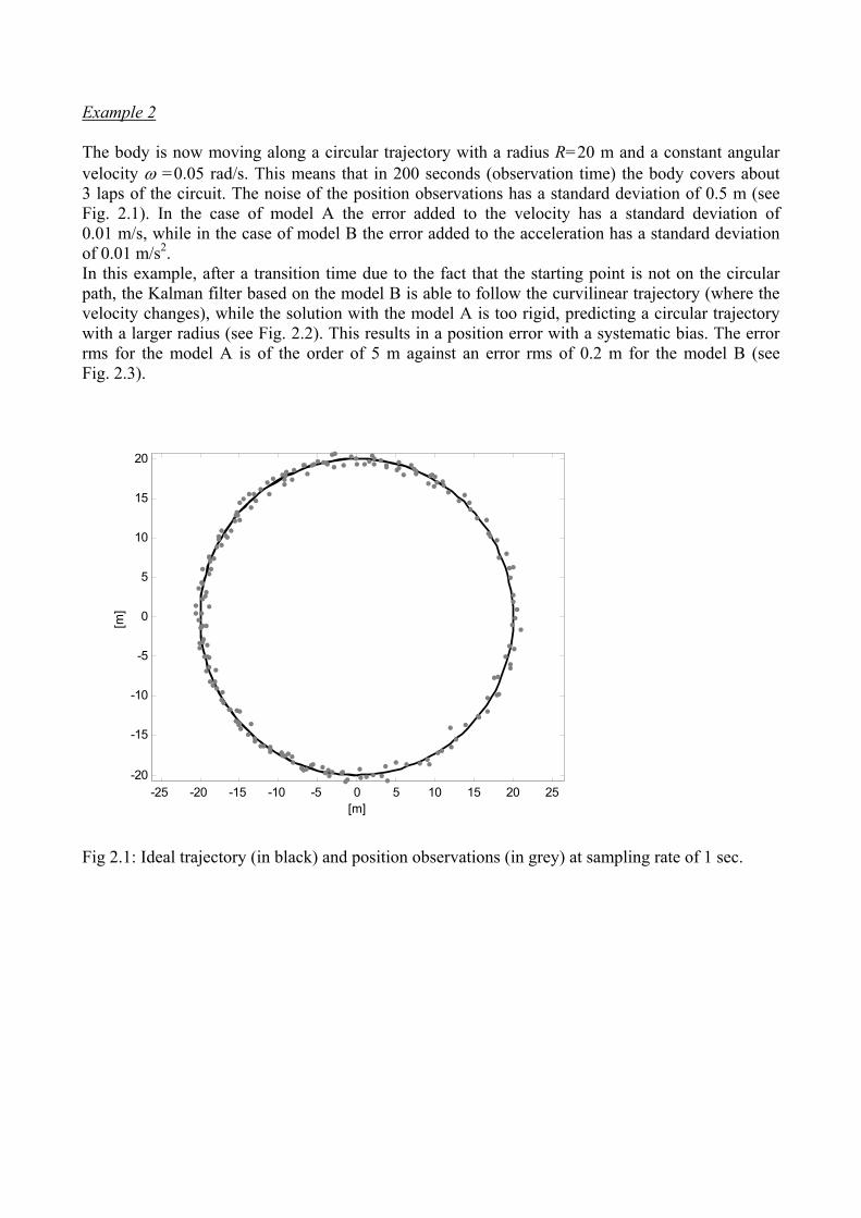
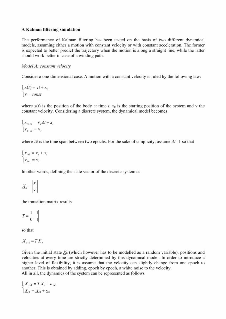
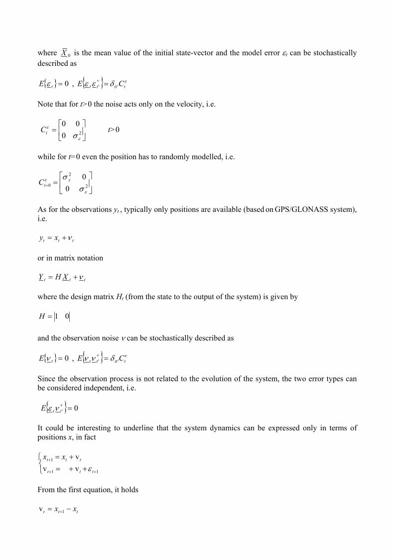
Example 2 The body is now moving along a circular trajectory with a radius R=20 m and a constant angular velocity ω =0.05 rad/s. This means that in 200 seconds (observation time) the body covers about 3 laps of the circuit. The noise of the position observations has a standard deviation of 0.5 m (see Fig. 2.1). In the case of model A the error added to the velocity has a standard deviation of 0.01 m/s, while in the case of model B the error added to the acceleration has a standard deviation of 0.01 m/s2. In this example, after a transition time due to the fact that the starting point is not on the circular path, the Kalman filter based on the model B is able to follow the curvilinear trajectory (where the velocity changes), while the solution with the model A is too rigid, predicting a circular trajectory with a larger radius (see Fig. 2.2). This results in a position error with a systematic bias. The error rms for the model A is of the order of 5 m against an error rms of 0.2 m for the model B (see Fig. 2.3).

-25 -20 -15 -10 -5 0 5 10 15 20 25-20

-15

-10

-5

0

5

10

15

20

[m]

[m]

Fig 2.1: Ideal trajectory (in black) and position observations (in grey) at sampling rate of 1 sec.

-25 -20 -15 -10 -5 0 5 10 15 20 25

-20

-15

-10

-5

0

5

10

15

20

[m]

[m]

Fig 2.2: Estimated trajectory using a Kalman filter with the dynamical model A (in black, solid line) and the dynamical model B (in grey, solid line). True trajectory in black dash line.

0 20 40 60 80 100 120 140 160 180 2000

0.5

1

1.5

2

2.5

3

3.5

4

4.5

5

time [s]

erro

r [m

]

Fig 2.3: Absolute value of the position errors using a Kalman filter with the dynamical model A (in black) and the dynamical model B (in grey).

Example 3 The body is moving along the path shown in Fig. 3.1. The observation noise has a standard deviation of 0.5 m. In the case of model A the error added to the velocity has a standard deviation of 0.005 m/s, while in the case of model B the error added to the acceleration has a standard deviation of 0.005 m/s2. This example emphasizes the pros and cons of the two models (see Fig. 3.2). In the straight stretches the solution A is more regular, but in the curvilinear sections it runs away from the true path; it needs some additional time to correct the trajectory when the road returns to be straight. On the other hand, the solution B is more “nervous” everywhere, but it is capable to follow the true trajectory even in the curvilinear sections. As a consequence, after the initial transition time, the error level become stable in the case of model B, while it oscillates in the case of model A, depending on the fact that the body is covering a straight or a curvilinear section (note that two of the four straight lines are not long enough to allow the body to come back on the right trajectory). The error rms for the model A is 1.2 m, while for the model B it is about 0.2 m (see Fig. 3.3). Example 4 The Example 3 is repeated along the same path and with the same observations, but now the error added to the velocity in the model A has a standard deviation of 0.05 m/s. In other words, higher model errors are accepted. The corresponding solution becomes much more reactive, following every change of direction. On the other hand, the main advantage of model A is definitively lost, since the trajectory has the same regularity of the one computed by using the model B. Therefore the two solutions are very similar (see Fig. 4.1), both with an error rms of 0.2 m (see Fig. 4.2).

-80 -70 -60 -50 -40 -30 -20 -10 0 10 20

-10

0

10

20

30

40

50

60

70

[m]

[m]

Fig 3.1: Ideal trajectory (in black) and position observations (in grey) at sampling rate of 1 sec.

-80 -60 -40 -20 0 20-20

-10

0

10

20

30

40

50

60

70

[m]

[m]

Fig 3.2: Estimated trajectory using a Kalman filter with the dynamical model A (in black, solid line) and the dynamical model B (in grey, solid line). True trajectory in black dash line.

0 50 100 150 200 250 3000

1

2

3

4

5

6

7

time [s]

erro

r [m

]

Fig 3.3: Absolute value of the position errors using a Kalman filter with the dynamical model A (in black) and the dynamical model B (in grey).

-80 -70 -60 -50 -40 -30 -20 -10 0 10 20

-10

0

10

20

30

40

50

60

70

[m]

[m]

Fig 4.1: Estimated trajectory using a Kalman filter with the dynamical model A (in black, solid line) and the dynamical model B (in grey, solid line). True trajectory in black dash line.

0 50 100 150 200 250 3000

0.5

1

1.5

2

2.5

3

3.5

time [s]

erro

r [s]

Fig 4.2: Absolute value of the position errors using a Kalman filter with the dynamical model A (in black) and the dynamical model B (in grey).

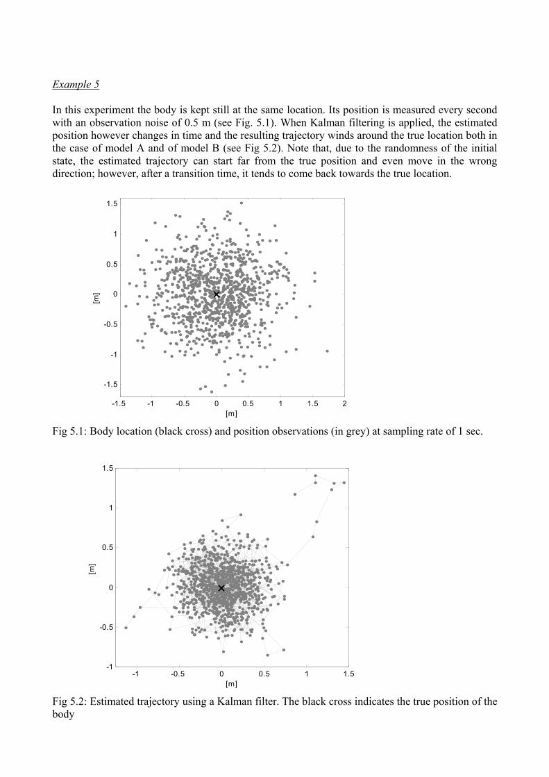
Example 5 In this experiment the body is kept still at the same location. Its position is measured every second with an observation noise of 0.5 m (see Fig. 5.1). When Kalman filtering is applied, the estimated position however changes in time and the resulting trajectory winds around the true location both in the case of model A and of model B (see Fig 5.2). Note that, due to the randomness of the initial state, the estimated trajectory can start far from the true position and even move in the wrong direction; however, after a transition time, it tends to come back towards the true location.

-1.5 -1 -0.5 0 0.5 1 1.5 2

-1.5

-1

-0.5

0

0.5

1

1.5

[m]

[m]

Fig 5.1: Body location (black cross) and position observations (in grey) at sampling rate of 1 sec.

-1 -0.5 0 0.5 1 1.5-1

-0.5

0

0.5

1

1.5

[m]

[m]

Fig 5.2: Estimated trajectory using a Kalman filter. The black cross indicates the true position of the body

Constrained Kalman filter Let us assume that the vehicle is constrained to cover a fixed path (e.g. a railway). Assume also that the path can be reasonably approximated by a broken line connecting some known points with coordinates (xi, yi) for i = 0,1,2,…,N. The distance between two consecutive points is given by

21

21,1 )()( −−− −+−= iiiiii yyxxd for i = 1,2,…,N

The distance between each point and the origin (x0, y0), computed along the broken line, can be written as

==

=

∑=

− Nids

si

jjji ,...,2,1for

0

1,1

0

Then, the path can be mathematically described as

−−

+=

−−

+=

−−

−−

−−

−−

)(

)(

1,1

11

1,1

11

iii

iii

iii

iii

ssd

yyyy

ssd

xxxx

for si-1< s < si and i = 1,2,…,N

where s is a mono-dimensional coordinate representing the distance of the moving vehicle with respect to the origin (x0, y0) along the broken line.

(x0, y0)

(x1, y1) (x2, y2)

d0,1

d1,2 s (x3, y3) d2,3 In this way a motion on the plane (or in general on a 3D space) is reduced to a motion in a 1D space. When applying the Kalman filter, the state of the system is described as a function of the coordinate s. In the case of a dynamical model based on constant velocity, we have

++=+=

++

+

11

1

ttt

ttt

sssss

ε&&

&

where represents the variation of the s coordinate in the unit time, i.e. the “velocity” of s. In other words, the state vector is defined as

s&

t

tt s

sX

&=

and the transition matrix results

1011

=T

so that

tt XTX =+1 . In the case of a dynamical model based on constant acceleration, we have

++=++=

+=

++

+

+

11

1

1

ttt

ttt

ttt

sssss

sss

ε&&&&

&&&&

&

where & represents the “acceleration” of s. In other words, the corresponding state vector is s&

t

t

t

t

sss

X&&

&=

and the transition matrix is given by

100110011

=T

Now the observation equations describe the relation between the s coordinate and the observations, which are for example the Cartesian coordinates (xt , yt) on the plane at the time t. Therefore, we can write:

+=+=

tytt

txtt

yyxx

,0

,0

νν

where are the observed coordinates and (),( 00

tt yx ), ,, tytx νν the corresponding measurement noise. By recalling the equation describing the motion along the broken line, the previous observation equations can expressed as

+−

=−

+−

+−

=−

+−

−

−−

−

−−

−

−−

−

−−

tytii

iii

ii

iiit

txtii

iii

ii

iiit

sd

yys

dyy

yy

sd

xxs

dxx

xx

,,1

11

,1

11

0

,,1

11

,1

11

0

ν

ν for si-1< st < si and i = 1,2,…,N

or in matrix notation

ttt XHY ν+=

with

1,1

11

0

1,1

11

0

−−

−−

−−

−−

−+−

−+−

=i

ii

iiit

iii

iiit

t

sd

yyyy

sd

xxxx

Y

and

ty

txt

,

,

νν

ν =

As for the transformation matrix H, in the case of a model with constant velocity, it is equal to

0

0

,1

1

,1

1

ii

ii

ii

ii

dyy

dxx

H

−

−

−

−

−

−

=

while in the case of a model with constant acceleration, it holds that

00

00

,1

1

,1

1

ii

ii

ii

ii

dyy

dxx

H

−

−

−

−

−

−

=