Asymmetric Stochastic Volatility Models: Properties and EstimationI

Xiuping Maoa, Esther Ruiza,b,∗, Helena Veigaa,b,c, Veronika Czellard

aDepartment of Statistics, Universidad Carlos III de Madrid, Spain.bInstituto Flores de Lemus, Universidad Carlos III de Madrid, Spain.

cFinancial Research Center/UNIDE, Portugal.dDepartment of Economics, Finance and Control, EMLYON Business School, France.

Abstract

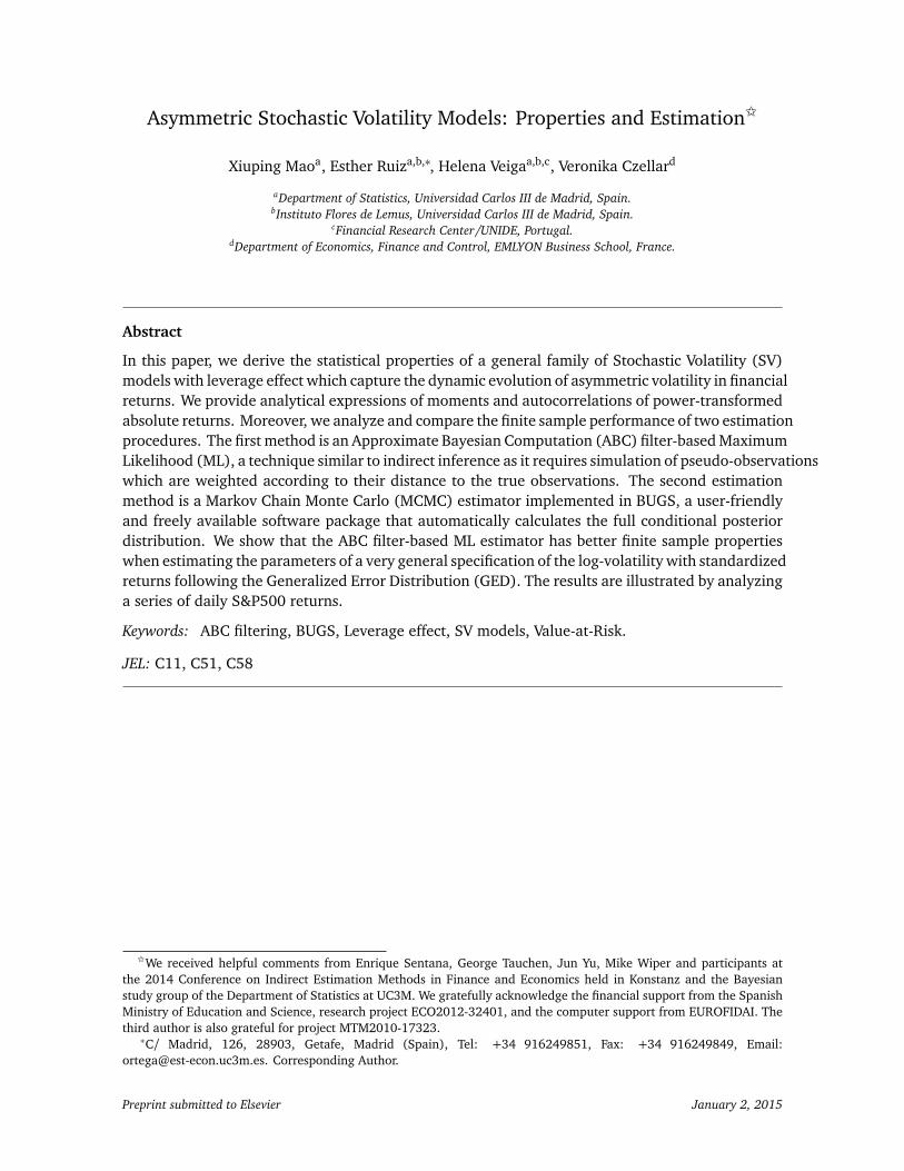
In this paper, we derive the statistical properties of a general family of Stochastic Volatility (SV)models with leverage effect which capture the dynamic evolution of asymmetric volatility in financialreturns. We provide analytical expressions of moments and autocorrelations of power-transformedabsolute returns. Moreover, we analyze and compare the finite sample performance of two estimationprocedures. The first method is an Approximate Bayesian Computation (ABC) filter-based MaximumLikelihood (ML), a technique similar to indirect inference as it requires simulation of pseudo-observationswhich are weighted according to their distance to the true observations. The second estimationmethod is a Markov Chain Monte Carlo (MCMC) estimator implemented in BUGS, a user-friendlyand freely available software package that automatically calculates the full conditional posteriordistribution. We show that the ABC filter-based ML estimator has better finite sample propertieswhen estimating the parameters of a very general specification of the log-volatility with standardizedreturns following the Generalized Error Distribution (GED). The results are illustrated by analyzinga series of daily S&P500 returns.

Keywords: ABC filtering, BUGS, Leverage effect, SV models, Value-at-Risk.

JEL: C11, C51, C58

IWe received helpful comments from Enrique Sentana, George Tauchen, Jun Yu, Mike Wiper and participants atthe 2014 Conference on Indirect Estimation Methods in Finance and Economics held in Konstanz and the Bayesianstudy group of the Department of Statistics at UC3M. We gratefully acknowledge the financial support from the SpanishMinistry of Education and Science, research project ECO2012-32401, and the computer support from EUROFIDAI. Thethird author is also grateful for project MTM2010-17323.

∗C/ Madrid, 126, 28903, Getafe, Madrid (Spain), Tel: +34 916249851, Fax: +34 916249849, Email:ortega@est-econ.uc3m.es. Corresponding Author.

Preprint submitted to Elsevier January 2, 2015

1. Introduction

Stochastic Volatility (SV) models, originally proposed by Taylor (1982, 1986) and popularized

by Harvey et al. (1994), specify the volatility of financial returns as a latent stochastic process.1

Asymmetric SV models incorporating the fact that volatility responds asymmetrically to past standardized

returns of different signs (leverage effect) have been introduced by Taylor (1994) and Harvey and

Shephard (1996).2 Even if normality of standardized returns is still a common assumption, SV

models with heavy-tailed and asymmetric distributions such as symmetric or skewed Student-t,

Generalized Error Distribution (GED)3 and mixtures of normals are increasingly popular (Liesenfeld

and Jung, 2000; Chen et al., 2008; Wang et al., 2011; Tsiotas, 2012).4

Although the literature on asymmetric SV models is rather extensive, the statistical properties

such as existence and analytical expressions of moments are known only in specific cases. For

instance, in an asymmetric SV model with Gaussian standardized returns proposed by Harvey and

Shephard (1996), Taylor (1994, 2007) provide expressions for the variance and kurtosis of returns

and the autocorrelation function of squared observations. Ruiz and Veiga (2008b) and Pérez

et al. (2009) derive the autocorrelation and cross-correlation functions of the power-transformed

absolute returns of an asymmetric autorregressive long memory SV model with Gaussian standardized

returns that nests the model proposed by Harvey and Shephard (1996). Asai and McAleer (2011)

derive the first and second order moments of returns generated by their general specification of

the volatility assuming normality of standardized returns. Eventually, Yu (2012a) also assumes

normality to derive the moments of returns and the conditions for stationarity, strict stationarity

and ergodicity of an asymmetric SV model with time-varying correlations.

However, the statistical properties are unknown in general asymmetric SV models in which the

standardized returns are not normally distributed. The first objective of this paper is to fill this gap

by deriving the properties of a very general family of asymmetric SV models with non-Gaussian

1See, for instance, Ghysels et al. (1996), Shephard (1996), Kim et al. (1998), Yu (2002) and Shephard (2005).2See also Breidt (1996), So et al. (2002), Bartolucci and De Luca (2003), McAleer (2005), Yu (2005), Yu et al. (2006),

Omori et al. (2007), Asai (2008), Asai and McAleer (2011), Tsiotas (2012) and Yu (2012a).3The GED distribution with parameter ν is described by Harvey (1990) and has the attractiveness of including

distributions with different tail thickness as, for example, the normal when ν = 2, the double exponential when ν = 1and the uniform distribution when ν=∞. The GED distribution has heavy tails if ν < 2.

4See also Cappuccio et al. (2004), Asai (2008), Choy et al. (2008), Asai and McAleer (2011), Nakajima and Omori(2012) and Wang et al. (2013).

2

standardized returns, from now on referred to as Generalized Asymmetric SV (GASV) family. In

particular, we provide general conditions for stationarity and for the existence of integer moments

of returns and absolute returns. In addition, we derive analytical expressions of the marginal

variance and kurtosis, the autocorrelations of power-transformed absolute returns and the cross-correlations

between returns and future power-transformed absolute returns for a given general specification

of the volatility with GED standardized returns.

Due to the intractability of the likelihood, parameter estimation in GASV models is a rather

difficult task.5 SV models with Gaussian errors have been estimated via a variety of methods

including the generalized method of moments (Taylor, 1986; Melino and Turnbull, 1990), indirect

inference (Gourieroux et al., 1993; Monfardini, 1998; Dhaene, 2004), quasi-maximum likelihood

(Harvey et al., 1994; Ruiz, 1994) and MCMC methods (Jacquier et al., 1994; Chib et al., 2002).6

However, to our knowledge, the estimation of a general specification of the GASV family with GED

standardized returns has not been covered in the literature yet.

The second goal of this paper is to provide estimation methods for this general setting. We use

an Approximate Bayesian Computation (ABC) filter-based Maximum Likelihood (ML) technique

proposed by Calvet and Czellar (2014). This procedure shares similarities with indirect inference

as it requires simulation of pseudo-observations which are weighted according to their distance to

the true observations. The hidden Markov states are sequentially simulated and resampled using a

Multinomial distribution. Due to the resampling step, the original ABC-filter estimated likelihood

is highly discontinuous which challenges maximum likelihood estimation. We smoothen the ABC

filtered likelihood by adopting Malik and Pitt (2011)’s continuous sampling method. This novel

continuous ABC filter greatly facilitates estimation via ML in complex state-space models such as

GASV models.

Our second estimation method is a MCMC procedure (Jacquier et al., 1994; Kim et al., 1998),

5See, for example, the surveys on the estimation of SV models by Broto and Ruiz (2004) and Yu (2012b).6Further methods include quadrature-based maximum likelihood estimation (Bartolucci and De Luca, 2003),

simulated maximum likelihood (Durham, 2006, 2007; Huang and Yu, 2008; Koopman et al., 2009; Skaug and Yu,2014), monte carlo likelihood (Sandmann and Koopman, 1998; Asai and McAleer, 2005; Jungbacker and Koopman,2007; Asai, 2008) and efficient importance sampling (Liesenfeld and Richard, 2003, 2006; Bauwens and Rombouts,2004; Asai and McAleer, 2011).

3

which is very popular to estimate parameters in SV models.7 In this paper, we use the MCMC

estimator implemented in the user-friendly and freely available BUGS software described in Meyer

and Yu (2000). This estimator is based on a single-move Gibbs sampling algorithm and has been

recently implemented in the context of asymmetric SV models by, for example, Yu (2012a) and

Wang et al. (2013). The MCMC estimator implemented in BUGS is appealing because it can handle

non-Gaussian level disturbances without much programming effort.

We compare the finite sample properties of the ABC filter-based ML and MCMC estimators.

We show that the MCMC estimator has difficulties while the ABC filter-based ML estimator is able

to estimate all parameters of the general framework paying a price in terms of programming and

computation time.

We also illustrate the performance of both estimation methods on a series of daily S&P500

returns observed between September 1998 and July 2014. We provide Value-at-Risk forecasts for

the out-of-sample period of August-December 2014.

The rest of the paper is organized as follows. In Section 2, we establish notation by describing

the general framework for SV models with leverage effect and derive its statistical properties.

Section 3 presents the popular asymmetric SV models that are contained in the GASV family and

derives analytical expressions of their moments. Section 4 describes the two alternative estimators

and reports the finite sample comparison of these estimators in Monte Carlo simulations. Section 5

presents an empirical application to daily S&P500 returns. Finally, the main conclusions and some

guidelines for future research are summarized in Section 6.

2. Statistical properties of GASV models

2.1. Model description

Let yt be the return at time t, σ2t its volatility, ht ≡ logσ2

t and εt be an independent and

identically distributed (IID) sequence with mean zero and variance one. The GASV family is given

by

yt = exp(ht/2)εt , t = 1, . . . , T (1)

7See Chib (2001) and Asai (2005) for good surveys and the contributions of Watanabe and Omori (2004); Omoriet al. (2007); Omori and Watanabe (2008); Nakajima and Omori (2009); Abanto-Valle et al. (2010) and Tsiotas (2012).

4

ht −µ= φ(ht−1 −µ) + f (εt−1) +ηt−1, (2)

where the log-volatility disturbance ηt−1 is a Gaussian white noise with variance σ2η

8 and f (εt−1)

is any function of εt−1 independent of ηt−1 for all leads and lags. The scale parameter µ determines

the marginal variance of returns, whileφ controls the rate of decay towards zero of the autocorrelations

of power-transformed absolute returns, hence, the persistence in volatility shocks. Note that, in

equations (1) and (2), the standardized return at time t −1 is correlated with the volatility at time

t. Furthermore, if f (·) is not an even function, then positive and negative past standardized returns

with the same magnitude have different effects on volatility.

It is important to note that although the specification of log-volatility in (2) is rather general,

it rules out models in which the persistence, φ, and/or the variance of the volatility noise, σ2η,

are time-varying.9 Finally, note that the only assumption made about the distribution of the level

disturbance, εt , is that it is an IID sequence with mean zero and variance one. As a consequence,

εt is strictly stationary.

2.2. Moments of returns

We now derive the statistical properties of the GASV family in equations (1) and (2). Theorem 2.1

establishes sufficient conditions for the stationarity of yt and derives the expression of E(y ct ) and

E(|yt |c) for any positive integer c.

Theorem 2.1. Consider a GASV process yt defined in equations (1) and (2). The process yt is strictly

stationary if |φ|< 1. Furthermore, if εt follows a distribution such that both E(exp(0.5c f (εt))) and

E(|εt |c) exist and are finite for some positive integer c, then {yt} and {|yt |} have finite, time-invariant

moments of order c given by

E(y ct ) = exp

� cµ2

�

E(εct)exp

�

c2σ2η

8(1−φ2)

�

P(0.5c,φ), (3)

8The normal assumption for ηt when f (εt−1) = 0 is justified in Andersen et al. (2001b) and Andersen et al. (2001a,2003).

9This excludes from the GASV family the time-varying specification of Yu (2012a).

5

and

E(|yt |c) = exp� cµ

2

�

E(|εt |c)exp

�

c2σ2η

8(1−φ2)

�

P(0.5c,φ), (4)

where P(a, b)≡∏∞

i=1 E(exp(abi−1 f (εt−i))).

Proof. See Appendix A.1.

Theorem 2.1 establishes the strict stationarity of yt if |φ| < 1; note that this is the same

condition derived by Yu (2012a) in his time-varying correlation model. The existence of the

expectation of y2t is guaranteed if, in addition, E(exp( f (εt))) <∞. Consequently, under these

two conditions, yt is also weakly stationary.

Note that according to expression (3), if εt has a symmetric distribution, then all odd moments

of yt are zero. Furthermore, from expression (4), it is straightforward to obtain expressions of the

marginal variance and kurtosis of yt as the following corollaries show.

Corollary 2.1. Under the conditions of Theorem 2.1 with c = 2 and taking into account that E(yt) =

0, the marginal variance of yt is directly obtained from (4) as follows

σ2y = exp

�

µ+σ2η

2(1−φ2)

�

P(1,φ). (5)

Corollary 2.2. Under the conditions of Theorem 2.1 with c = 4, the kurtosis of yt can be obtained as

E(y4t )/(E(y

2t ))

2 using expression (4) with c = 4 and c = 2 as follows

κy = κε exp

�

σ2η

1−φ2

�

P(2,φ)(P(1,φ))2

, (6)

where κε is the kurtosis of εt .

The kurtosis of the basic symmetric Autoregressive SV (ARSV) model considered by Taylor

(1982, 1986) and Harvey et al. (1994) is given by κε exp�

σ2η

1−φ2

�

. Therefore, this kurtosis is

multiplied by the factor r = P(2,φ)(P(1,φ)2 in the GASV family.

Note that, the expression of E(|yt |c) in (4) depends on the distribution of εt and f (·). Therefore,

in order to obtain closed-form expressions of the variance and kurtosis of returns, one needs to

6

assume a particular distribution of εt and specify f (εt). We will provide analytical expressions for

some popular distributions and specifications in Section 3. Note that even in cases in which the

function f (·) and/or the distribution of εt are such that they do not lead to obtain closed-form

expressions for the moments, expression (4) can always be used to simulate them as far as they are

finite.

2.3. Dynamic dependence

It is easy to see that returns generated from (1) and (2) are a martingale difference. However,

they are not serially independent as the conditional heteroscedasticity generates non-zero autocorrelations

of power-transformed absolute returns. The following theorem derives the autocorrelation function

(acf) of power transformed absolute returns.

Theorem 2.2. Consider a stationary process yt defined in equations (1) and (2) with |φ| < 1. If εt

follows a distribution such that E(exp(0.5c f (εt))) <∞ and E(|εt |c) <∞ for some positive integer

c, then the τ-th order autocorrelation of |yt |c is finite and given by

ρc(τ) =E(|εt |c)E(|εt |c exp(0.5cφτ−1 f (εt )))exp

�

φτc2σ2η

4(1−φ2)

�

P(0.5c(1+φτ),φ)Tτ(0.5c,φ)−[E(|εt |c)P(0.5c,φ)]2

E(|εt |2c)exp

�

c2σ2η

4(1−φ2)

�

P(c,φ)−[E(|εt |c)P(0.5c,φ)]2, (7)

where Tn(a, b)≡n−1∏

i=1

E(exp(abi−1 f (εt−i))) if n> 1 while T1(a, b)≡ 1.

Proof. See Appendix A.2.

Notice that, in practice, most authors dealing with real time series of financial returns focus on

the autocorrelations of squares, ρ2(τ), which can be obtained from (7) when c = 2.

The leverage effect is reflected in the cross-correlations between power-transformed absolute

returns and lagged returns. The following theorem gives general expressions of these cross-correlations.

Theorem 2.3. Consider a stationary process yt defined in equations (1) and (2) with |φ| < 1. If εt

follows a distribution such that E(exp(0.5c f (εt)))<∞ and E(|εt |2c)<∞ for some positive integer

7

c, then the τ-th order cross-correlation between yt and |yt+τ|c for τ > 0 is finite and given by

ρc1(τ) =E(|εt |c)exp

�

2cφτ−18(1−φ2)

σ2η

�

E(εt exp(0.5cφτ−1 f (εt )))P(0.5(1+cφτ),φ) Tτ(0.5c,φ)pP(1,φ)

√

√

√

E(|εt |2c)exp

�

c2σ2η

4(1−φ2)

�

P(c,φ)−[E(|εt |c)P(0.5c,φ)]2. (8)

Proof. See Appendix A.3.

Besides the cross-correlations between returns and future power-transformed absolute returns,

another useful tool to describe the asymmetric response of volatility is the News Impact Curve (NIC)

originally proposed by Engle and Ng (1993) in the context of GARCH models. The NIC is defined

as the function relating past return shocks to current volatility with all lagged conditional variances

evaluated at the unconditional variance of returns. Note that when referring to conditional variances,

we refer to the variance of returns at time t conditional on past returns observed up to and including

time t-1. The NIC has been widely implemented when dealing with GARCH-type models; see, for

example, Maheu and McCurdy (2004). Extending the NIC to SV models is not straightforward

due to the presence of the volatility disturbance in the latter models. As far as we know, there

are two attempts in the literature to propose a NIC function for SV models. The first is attributed

to Yu (2012a) who proposes a function that relates the conditional variance to the lagged return

innovation, εt−1, holding all other lagged returns equal to zero. Given that, in SV models the

conditional variance is not directly specified, this definition of the NIC requires solving high-dimensional

integrals using numerical methods. The second attempt is due to Takahashi et al. (2013) who

specify the news impact function for SV models in the spirit of Yu (2012a) as the volatility at time

t + 1 conditional on returns at time t. However, in order to obtain a U-shaped NIC, Takahashi

et al. (2013) propose to incorporate the dependence between returns and volatility by considering

their joint distribution. This idea is implemented by using a Bayesian MCMC scheme or a simple

rejection sampling.

It is important to note that, in the context of GARCH models, because there is just one disturbance,

the volatility at time t,σ2t , coincides with the conditional variance, Var(yt |y1, · · · , yt−1). Consequently,

when Engle and Ng (1993) propose relating past returns to current volatility, this amounts to

relating past returns with conditional variances. However, in SV models, the volatility, σ2t , and the

8

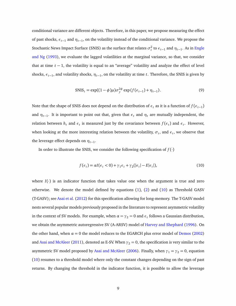
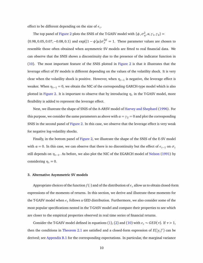
conditional variance are different objects. Therefore, in this paper, we propose measuring the effect

of past shocks, εt−1 and ηt−1, on the volatility instead of the conditional variance. We propose the

Stochastic News Impact Surface (SNIS) as the surface that relates σ2t to εt−1 and ηt−1. As in Engle

and Ng (1993), we evaluate the lagged volatilities at the marginal variance, so that, we consider

that at time t − 1, the volatility is equal to an “average” volatility and analyze the effect of level

shocks, εt−1, and volatility shocks, ηt−1, on the volatility at time t. Therefore, the SNIS is given by

SNISt = exp((1−φ)µ)σ2φy exp ( f (εt−1) +ηt−1) . (9)

Note that the shape of SNIS does not depend on the distribution of εt as it is a function of f (εt−1)

and ηt−1. It is important to point out that, given that εt and ηt are mutually independent, the

relation between ht and εt is measured just by the covariance between f (εt) and εt . However,

when looking at the more interesting relation between the volatility, σt , and εt , we observe that

the leverage effect depends on ηt−1.

In order to illustrate the SNIS, we consider the following specification of f (·)

f (εt) = αI(εt < 0) + γ1εt + γ2(|εt | − E|εt |), (10)

where I(·) is an indicator function that takes value one when the argument is true and zero

otherwise. We denote the model defined by equations (1), (2) and (10) as Threshold GASV

(T-GASV); see Asai et al. (2012) for this specification allowing for long-memory. The T-GASV model

nests several popular models previously proposed in the literature to represent asymmetric volatility

in the context of SV models. For example, when α= γ2 = 0 and εt follows a Gaussian distribution,

we obtain the asymmetric autoregressive SV (A-ARSV) model of Harvey and Shephard (1996). On

the other hand, when α= 0 the model reduces to the EGARCH plus error model of Demos (2002)

and Asai and McAleer (2011), denoted as E-SV. When γ2 = 0, the specification is very similar to the

asymmetric SV model proposed by Asai and McAleer (2006). Finally, when γ1 = γ2 = 0, equation

(10) resumes to a threshold model where only the constant changes depending on the sign of past

returns. By changing the threshold in the indicator function, it is possible to allow the leverage

9

effect to be different depending on the size of εt .

The top panel of Figure 2 plots the SNIS of the T-GASV model with {φ,σ2η,α,γ1,γ2}=

{0.98, 0.05,0.07,−0.08,0.1} and exp((1 − φ)µ)σ2φy = 1. These parameter values are chosen to

resemble those often obtained when asymmetric SV models are fitted to real financial data. We

can observe that the SNIS shows a discontinuity due to the presence of the indicator function in

(10). The most important feature of the SNIS plotted in Figure 2 is that it illustrates that the

leverage effect of SV models is different depending on the values of the volatility shock. It is very

clear when the volatility shock is positive. However, when ηt−1 is negative, the leverage effect is

weaker. When ηt−1 = 0, we obtain the NIC of the corresponding GARCH-type model which is also

plotted in Figure 2. It is important to observe that by introducing ηt in the T-GASV model, more

flexibility is added to represent the leverage effect.

Next, we illustrate the shape of SNIS of the A-ARSV model of Harvey and Shephard (1996). For

this purpose, we consider the same parameters as above withα= γ2 = 0 and plot the corresponding

SNIS in the second panel of Figure 2. In this case, we observe that the leverage effect is very weak

for negative log-volatility shocks.

Finally, in the bottom panel of Figure 2, we illustrate the shape of the SNIS of the E-SV model

with α = 0. In this case, we can observe that there is no discontinuity but the effect of εt−1 on σt

still depends on ηt−1. As before, we also plot the NIC of the EGARCH model of Nelson (1991) by

considering ηt = 0.

3. Alternative Asymmetric SV models

Appropriate choices of the function f (·) and of the distribution of εt allow us to obtain closed-form

expressions of the moments of returns. In this section, we derive and illustrate these moments for

the T-GASV model when εt follows a GED distribution. Furthermore, we also consider some of the

most popular specifications nested in the T-GASV model and compare their properties to see which

are closer to the empirical properties observed in real time series of financial returns.

Consider the T-GASV model defined in equations (1), (2) and (10) with εt ∼ GED(ν). If ν > 1,

then the conditions in Theorem 2.1 are satisfied and a closed-form expression of E(|yt |c) can be

derived; see Appendix B.1 for the corresponding expectations. In particular, the marginal variance

10

of yt is given by equation (5) with

P(1,φ) =∏∞

i=1

§

∑∞k=0

�

�

Γ (1/ν)Γ (3/ν)

�k/2 Γ ((k+1)/ν)2Γ (1/ν)k! φ

k(i−1)�

(γ1 + γ2)k + exp(αφ i−1)(γ2 − γ1)k�

�ª

,

(11)

where Γ (·) is the Gamma function. Note that in order to compute P(·, ·), one needs to truncate the

corresponding infinite product and summation. Our experience is that truncating the product at

i = 500 and the summation at k = 1000 gives very stable results. We can calculate the kurtosis in

(6) in a similar way.

Given that the Gaussian distribution is a special case of the GED distribution when ν = 2,

closed-form expressions of E(|yt |c) can also be obtained in this case; see Appendix B.2 for the

corresponding expectations.10 In particular, the marginal variance is given by expression (5) while

the kurtosis is given by expression (6) with

P(1,φ) =∏∞

i=1

n

exp�

αφ i−1 + φ2i−2(γ1−γ2)2

2

�

Φ(φ i−1(γ2 − γ1)) + exp�

φ2i−2(γ1+γ2)2

2

�

Φ(φ i−1(γ2 + γ1))o

,

(12)

whereΦ(·) is the Gaussian cumulative distribution function. The expression of the marginal variance

derived by Taylor (1994) for the classical asymmetric SV model of Harvey and Shephard (1996),

by Ruiz and Veiga (2008a) for the asymmetric long-memory SV model and by Asai and McAleer

(2011) for their general specification can be obtained as particular cases of expression (5) with

P(1,φ) defined as in (12).

When ν < 1, we cannot obtain analytical expressions of E(|yt |c). However, in Appendix B.1,

we show that, in this case, E(|yt |c) in equation (4) is finite if γ2+γ1 ≤ 0 and γ2−γ1 ≤ 0.11 Finally,

if ν = 1, the conditions for the existence of E(|yt |c) in equation (4) are γ2 + γ1 < 2p

2/c and

γ2 − γ1 < 2p

2/c.

The expectations needed to obtain closed-form expressions of the autocorrelations in expression

10These expectations are derived by Demos (2002) when p = 0 or 1 and α= 0.11The same conditions should be satisfied for the finiteness of E(|yt |c) when εt follows a Student-t distribution with

d > 2 degrees of freedom.

11

(7) and cross-correlations in (8) have been derived in Appendix B.1 for the T-GASV model with

parameter ν > 1 and in Appendix B.2 for the particular case of the Gaussian distribution, i.e. ν= 2.

As above, when ν≤ 1, we can only obtain conditions for the existence of the autocorrelations and

cross-correlations. As these autocorrelations are highly non-linear functions of the parameters, it

is not straightforward to analyze the role of each parameter on their shape. Consequently, in order

to illustrate how these moments depend on each of the parameters, we focus on the model with

parameters φ = 0.98, σ2η = 0.05 and Gaussian errors.

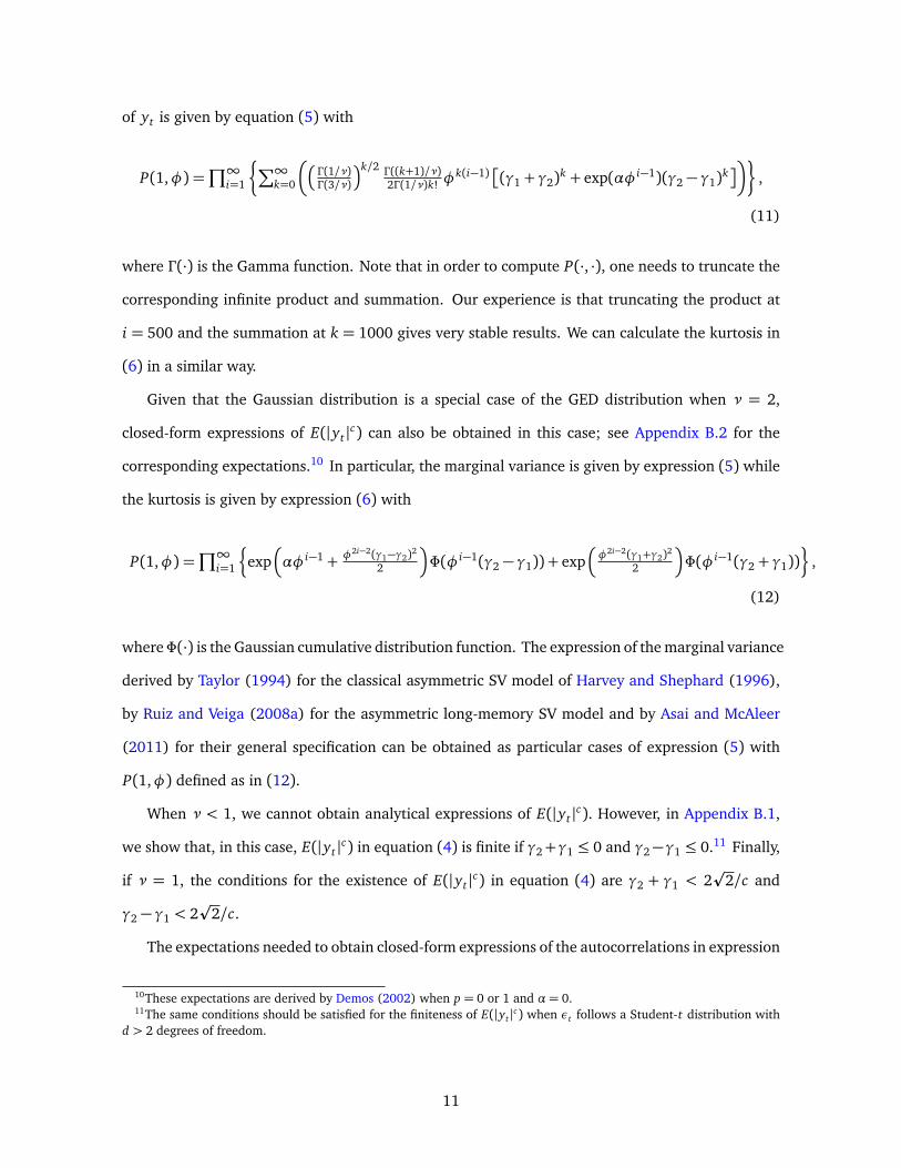
The first order autocorrelations of squared returns, namely, ρ2(1), is plotted in the first panel of

Figure 3 as a function of the leverage parameters, γ1 and α. We observe that the autocorrelations

of squared returns are larger for larger values of γ2. However, both surfaces are rather flat and,

consequently, the leverage parameters do not have large effects on the first order autocorrelations

of squares.

In the second panel of Figure 3, we illustrate the effect of the parameters on the cross-correlations

between yt and y2t+1 denoted by ρ21(1). Observe that the first order cross-correlations between

returns and future squared returns are indistinguishable for the two values of γ2 considered in

Figure 3. |γ1| drags ρ21(1) in an approximately linear way while the effect of α is non-linear.

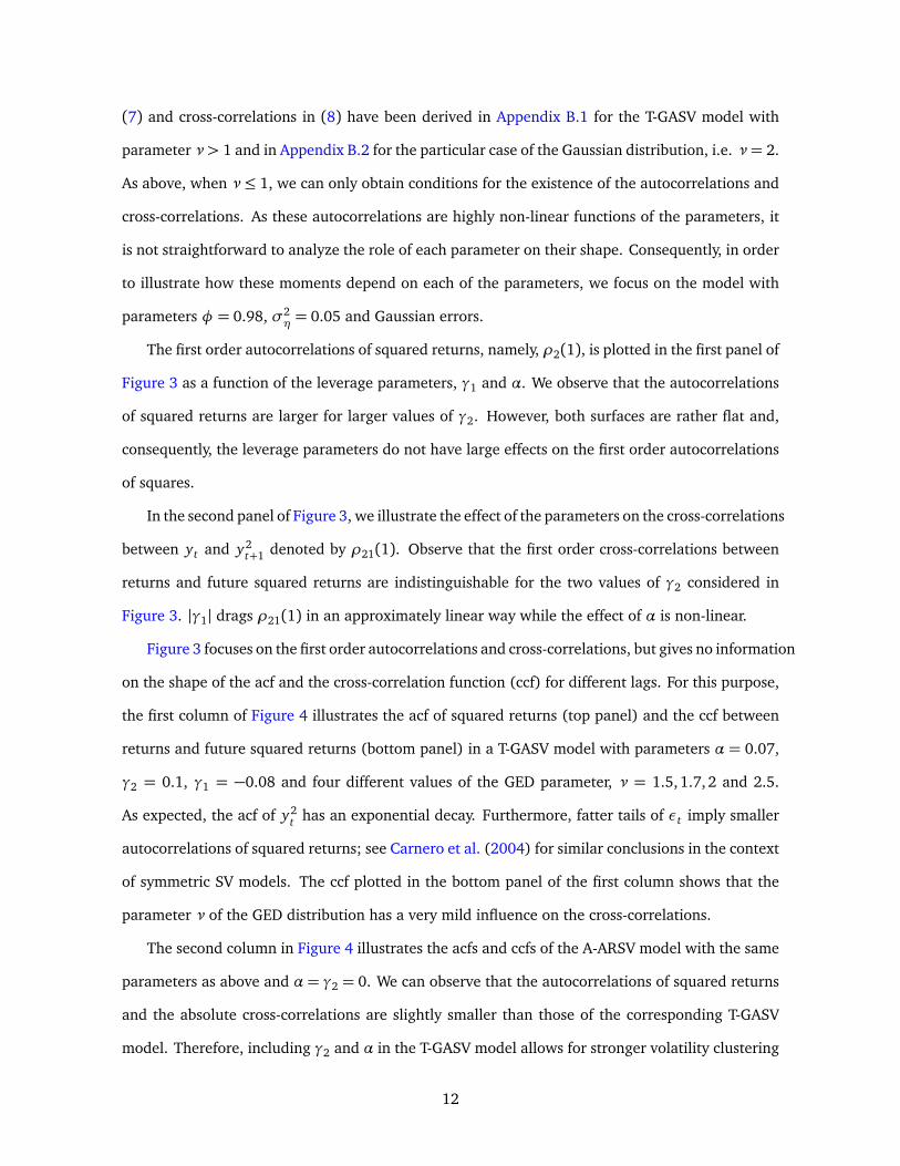
Figure 3 focuses on the first order autocorrelations and cross-correlations, but gives no information

on the shape of the acf and the cross-correlation function (ccf) for different lags. For this purpose,

the first column of Figure 4 illustrates the acf of squared returns (top panel) and the ccf between

returns and future squared returns (bottom panel) in a T-GASV model with parameters α = 0.07,

γ2 = 0.1, γ1 = −0.08 and four different values of the GED parameter, ν = 1.5,1.7, 2 and 2.5.

As expected, the acf of y2t has an exponential decay. Furthermore, fatter tails of εt imply smaller

autocorrelations of squared returns; see Carnero et al. (2004) for similar conclusions in the context

of symmetric SV models. The ccf plotted in the bottom panel of the first column shows that the

parameter ν of the GED distribution has a very mild influence on the cross-correlations.

The second column in Figure 4 illustrates the acfs and ccfs of the A-ARSV model with the same

parameters as above and α= γ2 = 0. We can observe that the autocorrelations of squared returns

and the absolute cross-correlations are slightly smaller than those of the corresponding T-GASV

model. Therefore, including γ2 and α in the T-GASV model allows for stronger volatility clustering

12

and leverage effect.

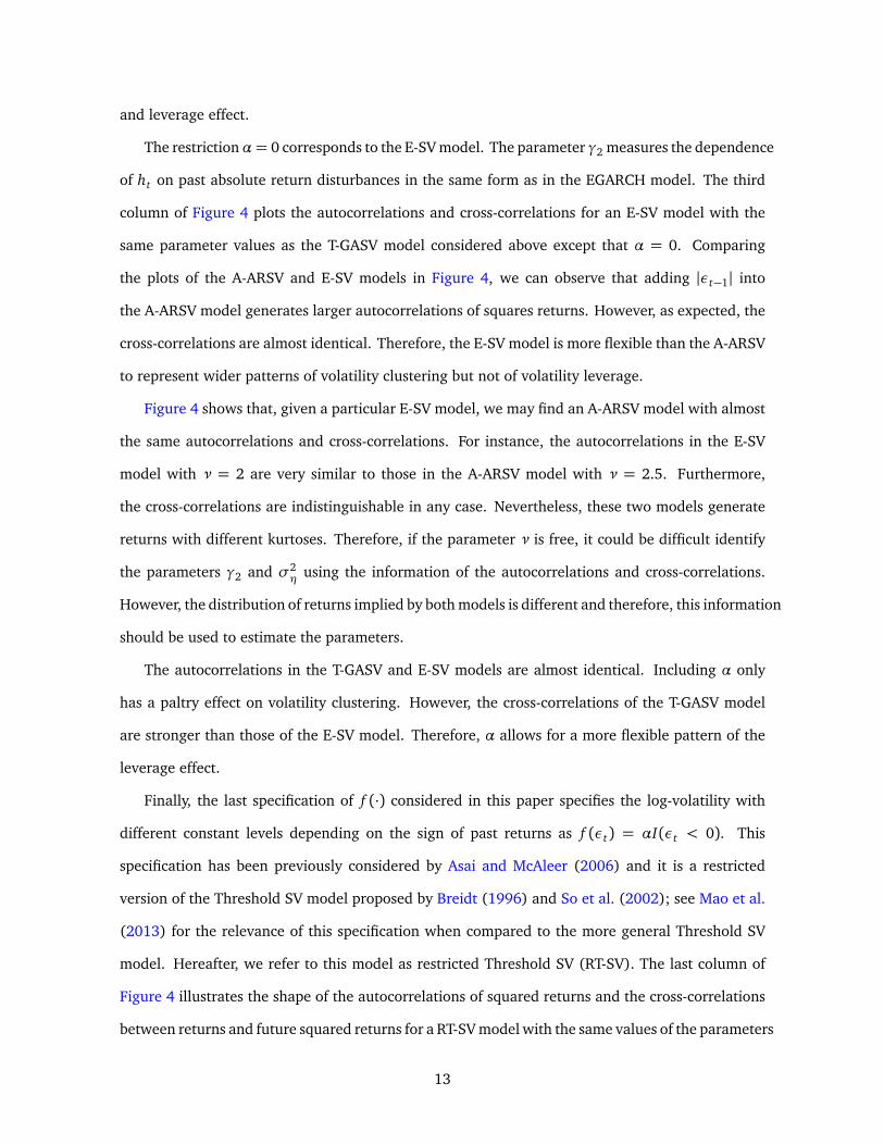
The restrictionα= 0 corresponds to the E-SV model. The parameter γ2 measures the dependence

of ht on past absolute return disturbances in the same form as in the EGARCH model. The third

column of Figure 4 plots the autocorrelations and cross-correlations for an E-SV model with the

same parameter values as the T-GASV model considered above except that α = 0. Comparing

the plots of the A-ARSV and E-SV models in Figure 4, we can observe that adding |εt−1| into

the A-ARSV model generates larger autocorrelations of squares returns. However, as expected, the

cross-correlations are almost identical. Therefore, the E-SV model is more flexible than the A-ARSV

to represent wider patterns of volatility clustering but not of volatility leverage.

Figure 4 shows that, given a particular E-SV model, we may find an A-ARSV model with almost

the same autocorrelations and cross-correlations. For instance, the autocorrelations in the E-SV

model with ν = 2 are very similar to those in the A-ARSV model with ν = 2.5. Furthermore,

the cross-correlations are indistinguishable in any case. Nevertheless, these two models generate

returns with different kurtoses. Therefore, if the parameter ν is free, it could be difficult identify

the parameters γ2 and σ2η using the information of the autocorrelations and cross-correlations.

However, the distribution of returns implied by both models is different and therefore, this information

should be used to estimate the parameters.

The autocorrelations in the T-GASV and E-SV models are almost identical. Including α only

has a paltry effect on volatility clustering. However, the cross-correlations of the T-GASV model

are stronger than those of the E-SV model. Therefore, α allows for a more flexible pattern of the

leverage effect.

Finally, the last specification of f (·) considered in this paper specifies the log-volatility with

different constant levels depending on the sign of past returns as f (εt) = αI(εt < 0). This

specification has been previously considered by Asai and McAleer (2006) and it is a restricted

version of the Threshold SV model proposed by Breidt (1996) and So et al. (2002); see Mao et al.

(2013) for the relevance of this specification when compared to the more general Threshold SV

model. Hereafter, we refer to this model as restricted Threshold SV (RT-SV). The last column of

Figure 4 illustrates the shape of the autocorrelations of squared returns and the cross-correlations

between returns and future squared returns for a RT-SV model with the same values of the parameters

13

as those considered above and γ1 = γ2 = 0. Comparing the autocorrelations of squaresd and

absolute returns in the T-GASV and the RT-SV models represented in the top panel, we observe

that the latter are slightly smaller than the former. However, the absolute cross-correlations in the

RT-SV model are the smallest among all the models considered. The presence of α in the T-GASV

model seems to reinforce the role of the leverage parameter γ1.

4. Model estimation

As shown in the previous section, GASV models are attractive because of their flexibility to

mimic the dynamic properties of financial return data. The downside to adopting an appealing

GASV model is the difficulty involved with parameter estimation and volatility forecasts. The

intractability of the likelihood is inherited from standard SV models, see Broto and Ruiz (2004)

and Yu (2012b) for surveys on estimation procedures for SV models.

In this paper, we consider two estimation methods for GASV models. The first one is an ABC

filter-based ML procedure proposed by Calvet and Czellar (2014), which closely relates to indirect

inference in the sense that it estimates the conditional distribution of the hidden-state, by a set of

particles which are able to generate pseudo-observations close to the real observations. The second

is the MCMC estimator described by Meyer and Yu (2000) who propose to estimate the A-ARSV

model using the user-friendly and freely available BUGS software. This estimator is attractive

because it reduces the computational effort. Furthermore, note that Bayesian MCMC does not rely

on asymptotic approximations to conduct inference.

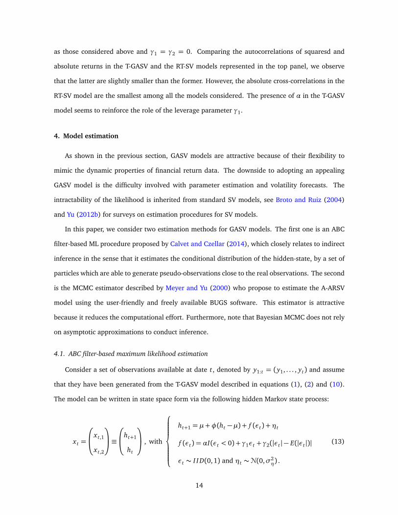
4.1. ABC filter-based maximum likelihood estimation

Consider a set of observations available at date t, denoted by y1:t = (y1, . . . , yt) and assume

that they have been generated from the T-GASV model described in equations (1), (2) and (10).

The model can be written in state space form via the following hidden Markov state process:

x t =

x t,1

x t,2

≡

ht+1

ht

, with

ht+1 = µ+φ(ht −µ) + f (εt) +ηt

f (εt) = αI(εt < 0) + γ1εt + γ2(|εt | − E(|εt |)|

εt ∼ I I D(0,1) and ηt ∼N(0,σ2η) .

(13)

14

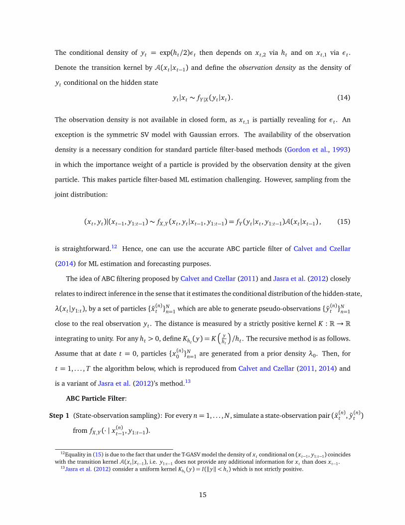
The conditional density of yt = exp(ht/2)εt then depends on x t,2 via ht and on x t,1 via εt .

Denote the transition kernel by A(x t |x t−1) and define the observation density as the density of

yt conditional on the hidden state

yt |x t ∼ fY |X (yt |x t) . (14)

The observation density is not available in closed form, as x t,1 is partially revealing for εt . An

exception is the symmetric SV model with Gaussian errors. The availability of the observation

density is a necessary condition for standard particle filter-based methods (Gordon et al., 1993)

in which the importance weight of a particle is provided by the observation density at the given

particle. This makes particle filter-based ML estimation challenging. However, sampling from the

joint distribution:

(x t , yt)|(x t−1, y1:t−1)∼ fX ,Y (x t , yt |x t−1, y1:t−1) = fY (yt |x t , y1:t−1)A(x t |x t−1) , (15)

is straightforward.12 Hence, one can use the accurate ABC particle filter of Calvet and Czellar

(2014) for ML estimation and forecasting purposes.

The idea of ABC filtering proposed by Calvet and Czellar (2011) and Jasra et al. (2012) closely

relates to indirect inference in the sense that it estimates the conditional distribution of the hidden-state,

λ(x t |y1:t), by a set of particles { x (n)t }Nn=1 which are able to generate pseudo-observations { y(n)t }

Nn=1

close to the real observation yt . The distance is measured by a strictly positive kernel K : R→ R

integrating to unity. For any ht > 0, define Kht(y) = K

�

yht

�

/ht . The recursive method is as follows.

Assume that at date t = 0, particles {x (n)0 }Nn=1 are generated from a prior density λ0. Then, for

t = 1, . . . , T the algorithm below, which is reproduced from Calvet and Czellar (2011, 2014) and

is a variant of Jasra et al. (2012)’s method.13

ABC Particle Filter:

Step 1 (State-observation sampling): For every n= 1, . . . , N , simulate a state-observation pair ( x (n)t , y(n)t )

from fX ,Y (· | x(n)t−1, y1:t−1).

12Equality in (15) is due to the fact that under the T-GASV model the density of x t conditional on (x t−1, y1:t−1) coincideswith the transition kernel A(x t |x t−1), i.e. y1:t−1 does not provide any additional information for x t than does x t−1.

13Jasra et al. (2012) consider a uniform kernel Kht(y) = I(‖y‖< ht) which is not strictly positive.

15

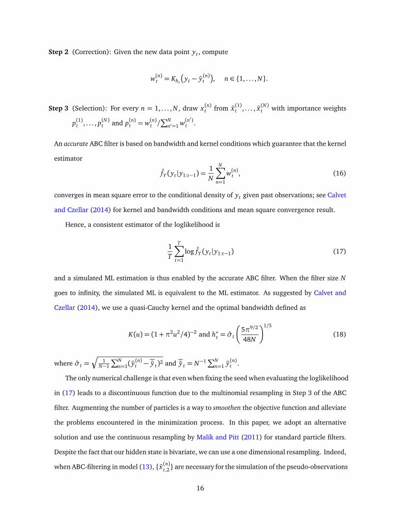
Step 2 (Correction): Given the new data point yt , compute

w(n)t = Kht

�

yt − y(n)t

�

, n ∈ {1, . . . , N}.

Step 3 (Selection): For every n = 1, . . . , N , draw x (n)t from x (1)t , . . . , x (N)t with importance weights

p(1)t , . . . , p(N)t and p(n)t = w(n)t /∑N

n′=1 w(n′)

t .

An accurate ABC filter is based on bandwidth and kernel conditions which guarantee that the kernel

estimator

fY (yt |y1:t−1) =1N

N∑

n=1

w(n)t , (16)

converges in mean square error to the conditional density of yt given past observations; see Calvet

and Czellar (2014) for kernel and bandwidth conditions and mean square convergence result.

Hence, a consistent estimator of the loglikelihood is

1T

T∑

t=1

log fY (yt |y1:t−1) (17)

and a simulated ML estimation is thus enabled by the accurate ABC filter. When the filter size N

goes to infinity, the simulated ML is equivalent to the ML estimator. As suggested by Calvet and

Czellar (2014), we use a quasi-Cauchy kernel and the optimal bandwidth defined as

K(u) = (1+π2u2/4)−2 and h∗t = σt

�

5π9/2

48N

�1/5

(18)

where σt =Ç

1N−1

∑Nn=1( y

(n)t − y t)2 and y t = N−1

∑Nn=1 y(n)t .

The only numerical challenge is that even when fixing the seed when evaluating the loglikelihood

in (17) leads to a discontinuous function due to the multinomial resampling in Step 3 of the ABC

filter. Augmenting the number of particles is a way to smoothen the objective function and alleviate

the problems encountered in the minimization process. In this paper, we adopt an alternative

solution and use the continuous resampling by Malik and Pitt (2011) for standard particle filters.

Despite the fact that our hidden state is bivariate, we can use a one dimensional resampling. Indeed,

when ABC-filtering in model (13), { x (n)t,2} are necessary for the simulation of the pseudo-observations

16

{ y(n)t } in Step 2, but {x (n)t,2} are ignored when generating { x (n)t+1} in step 1. Hence we can base our

resampling Step 3 on the first components { x (n)t,1} solely. The continuous resampling algorithm by

Malik and Pitt (2011) along with Malmquist (1950) ordered uniforms is summarized in Appendix

C.

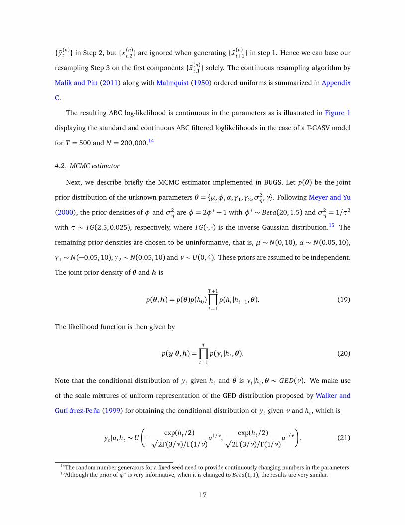
The resulting ABC log-likelihood is continuous in the parameters as is illustrated in Figure 1

displaying the standard and continuous ABC filtered loglikelihoods in the case of a T-GASV model

for T = 500 and N = 200, 000.14

4.2. MCMC estimator

Next, we describe briefly the MCMC estimator implemented in BUGS. Let p(θ) be the joint

prior distribution of the unknown parameters θ = {µ,φ,α,γ1,γ2,σ2η,ν}. Following Meyer and Yu

(2000), the prior densities of φ and σ2η are φ = 2φ∗ − 1 with φ∗ ∼ Beta(20,1.5) and σ2

η = 1/τ2

with τ ∼ IG(2.5,0.025), respectively, where IG(·, ·) is the inverse Gaussian distribution.15 The

remaining prior densities are chosen to be uninformative, that is, µ ∼ N(0, 10), α ∼ N(0.05, 10),

γ1 ∼ N(−0.05, 10), γ2 ∼ N(0.05,10) and ν∼ U(0,4). These priors are assumed to be independent.

The joint prior density of θ and h is

p(θ,h) = p(θ)p(h0)T+1∏

t=1

p(ht |ht−1,θ). (19)

The likelihood function is then given by

p(y|θ,h) =T∏

t=1

p(yt |ht ,θ). (20)

Note that the conditional distribution of yt given ht and θ is yt |ht ,θ ∼ GED(ν). We make use

of the scale mixtures of uniform representation of the GED distribution proposed by Walker and

Gutiérrez-Peña (1999) for obtaining the conditional distribution of yt given ν and ht , which is

yt |u, ht ∼ U

�

−exp(ht/2)

p

2Γ (3/ν)/Γ (1/ν)u1/ν,

exp(ht/2)p

2Γ (3/ν)/Γ (1/ν)u1/ν

�

, (21)

14The random number generators for a fixed seed need to provide continuously changing numbers in the parameters.15Although the prior of φ∗ is very informative, when it is changed to Beta(1,1), the results are very similar.

17

where u|ν ∼ Gamma(1 + 1/ν, 2−ν/2). Given the initial values (θ(0),h(0)), the Gibbs sampler

generates a Markov Chain for each parameter and volatility in the model through the following

steps:

θ(1)1 ∼ p(θ1|θ

(0)2 , . . . ,θ (0)K ,h(0),y);

...

θ(1)K ∼ p(θ1|θ

(1)2 , . . . ,θ (1)K−1,h(0),y);

h(1)1 ∼ p(h1|θ(1), h(0)2 , . . . , h(0)T+1,y);

...

h(1)T+1 ∼ p(hT+1|θ(1), h(1)1 , . . . , h(1)T ,y).

The estimates of the parameters and volatilities are the means of the Markov Chain. Finally, the

posterior joint distribution of the parameters and volatilities is given by

p(θ,h|y)∝ p(θ)p(h0)T+1∏

t=1

p(ht |ht−1,y,θ)T∏

t=1

p(yt |ht ,θ). (22)

4.3. Finite sample performance of the parameter estimators

In this section, we carry out extensive Monte Carlo experiments to analyze the finite sample

performance of the ABC filter-based ML and MCMC estimators when estimating the parameters

of the T-GASV model. We consider two designs for the Monte Carlo experiments. First, we treat

ν as known and estimate all other parameters in the model. In this case, R = 500 replicates are

generated by the T-GASV model with normal errors, parameters (µ,φ,α,γ1,γ2,σ2η) = (0, 0.98,0.07,−0.08,0.1, 0.05)

and sample sizes T = 500, 1000 and 2000. Second, R replicates are generated by the T-GASV

model with GED standardized returns with ν= 1.5. In this case, the parameter ν is also estimated.

For computational efficiency, we choose to estimate µ · (1 − φ) instead of µ in our estimation

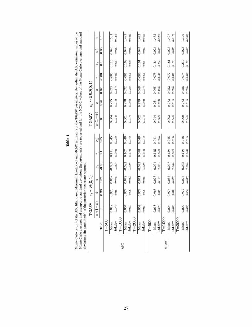
procedures. The top panel of Table 1 reports the Monte Carlo averages of the estimates and the

asymptotic standard deviations of the ABC filter-based ML estimates. The lower panel of Table 1

reports the Monte Carlo averages and standard deviations of the posterior means of the MCMC

estimates of the parameters.

18

Consider first the results obtained with the ABC filter-based ML estimator. We can observe that

regardless of whether the distribution of the standardized returns is assumed to be known, or not,

all the parameters are accurately estimated, even when the sample size is as small as T = 500.

The Monte Carlo averages of the asymptotic standard deviations of the parameter estimates decay

approximately at ratep

T . These Monte Carlo experiments show that the ABC filter-based ML

estimator does a remarkably good job in estimating the parameters of the general asymmetric SV

model considered in this paper.

Consider now the results regarding the MCMC estimator which are based on a total number of

20,000 iterations after a burn-in of 10,000.16 When the distribution of the standardized returns is

known, we can observe that the Monte Carlo averages of the posterior means are, in general, further

from the true parameters than are the ABC filter-based ML estimates. Standard deviations are also

larger. Obviously, as the sample size increases the differences between the ABC filter-based ML and

MCMC estimators disappear. However, even when T = 2000 the Monte Carlo standard errors of the

MCMC estimator are still much larger than those of the ABC filter-based ML estimator mainly for

the constant, µ · (1−φ), and the threshold, α, parameters. When the data are generated with GED

standardized returns (right panel), the Monte Carlo averages of the estimates of µ·(1−φ),φ, α and

γ1 are very similar to those obtained with known ν= 2 (left panel). However, the estimates of γ2,

σ2η and ν suffer from biases which do not disappear with the sample size. Moreover, the standard

deviations do not decrease with the sample size as expected. Both σ2η and ν are underestimated

while γ2 is overestimated. The correlation between the estimates of γ2 and σ2η is almost -0.7 while

the correlation between the estimates of ν and γ2 is as high as -0.8. When compared with the

standard deviations of the ABC filter-based ML estimator, the Monte Carlo standard deviations of

the posterior means of the MCMC estimator are approximately three times larger when T = 2000.

So the MCMC estimator is less successful in estimating the parameters γ2, σ2η and ν.17 However,

the MCMC estimator has a significant computational advantage. While an ABC filter-based ML

16The random number generators for a fixed seed need to provide continuously changing numbers in the parameters.For instance, the inverse cdf method satisfies this property.

17Skaug and Yu (2014) use 100000 draws while Omori et al. (2007) show that even few hundred thousand drawscannot be enough. For some particular cases, we increase the number of iterations to 75000 obtaining very similarresults.

19

estimation of a T-GASV model with T = 500 takes on average 2438 minutes to compile18, the

MCMC took only 11 minutes19. Hence, computation time is the price to pay for the accuracy gain

obtained via ABC filter-based ML estimator.

5. Empirical application

5.1. Data description and estimation results

In this section, we fit the T-GASV model to a series of daily S&P500 returns observed between

September 1, 1998 and December 17, 2014. We split the observation period into an in-sample

and an out-of-sample periods. The in-sample period ends on July 25, 2014 and contains T =

4000 observations. The out-of-sample period starts on July 28, 2014 and represents H = 101

observations. The returns are computed as yt = 100 × 4 log Pt , where Pt is the adjusted close

price at time t obtained from finance.yahoo.com. The adjusted close prices together with their

corresponding returns are plotted in Figure 5 for the in-sample period which suggests the presence

of volatility clustering with episodes of large volatility associated with periods of negative movements

in prices. Furthermore, this association between large volatility and negative returns is observed

in the negative sample cross-correlations between returns and future squared returns also plotted

in Figure 5.

We estimate the T-GASV model with GED standardized returns using both ABC filter-based ML

and MCMC estimators. Table 2 reports the estimates obtained using the observations corresponding

to the in-sample period. For the ABC filter-based ML estimates, we report asymptotic standard

errors in parentheses. Regarding the MCMC estimation, we report the posterior mean and the

posterior standard deviation of the MCMC estimator of each parameter. The plug-in ABC-filter

estimated loglikelihoods are also reported. Heteroskedasticity and autocorrelation consistent Vuong

test comparing the MCMC specification to the ABC filtered specification are reported in parentheses

below the log-likelihood value. The ABC filter-based loglikelihood is smaller for MCMC but the

difference is not significant at the 5% level according to the Vuong test. The estimates of ν are

18The computation was performed on an Intel(R) Xeon(R) CPU E5-2630 0 @ 2.30GHz.19The computation was performed on an Intel(R) Xeon(R) CPU E5-2665 0 @ 2.40GHz.

20

less than the value two for both estimation methods which indicates that the standardized returns

follow a fat-tailed distribution.

When using the ABC filter-based ML estimator, all parameters including the threshold are

statistically significant. Furthermore, except for φ, the ABC filter-based ML and MCMC estimates

are rather different with the asymptotic standard deviations of the ABC filter-based estimates being

smaller than the posterior standard deviations of the MCMC estimates. In concordance with the

Monte Carlo results, the MCMC estimate of γ2, seems to be overestimated while σ2η and ν are

underestimated.

Finally, Figure 5 plots the plug-in moments implied by the two estimators together with the

corresponding sample moments. The plug-in moments given by the ABC filter-based ML estimator

are slightly closer to the sample moments comparing with those of the corresponding MCMC

estimator.

5.2. Forecasting performance

In this subsection, we perform an out-of-sample comparison of the ability of the two alternative

estimation methods considered in this paper to calculate the one-step-ahead VaR of the daily

S&P500 returns using the T-GASV model with GED standardized returns. Given the extremely

heavy computations involved in the estimation of the ABC filter-based ML we use estimates provided

in Table 2 for the VaR forecasts in the entire out-of-sample period. We compute one-day-ahead VaR

forecasts from July 28, 2014, 2010 to December 17, 2014 as

VaRαt+1 = −qt,α, (23)

with α = 1%, 5% and 10% and qt,α are the quantiles of the distribution of yt+1|y1:t , which is

conveniently estimated by the ABC filter. We provide in total 101 one-step-ahead VaR forecasts.

In order to evaluate the adequacy of the VaR forecasts with both estimation methods, Table 2

reports the failure rates of the 101 VaR forecasts. The failure rates of the T-GASV model with

GED standardized returns are quite similar across the estimation methods and are not significantly

different from their theoretical values at the 5% significance level. For the 5% VaR, the empirical

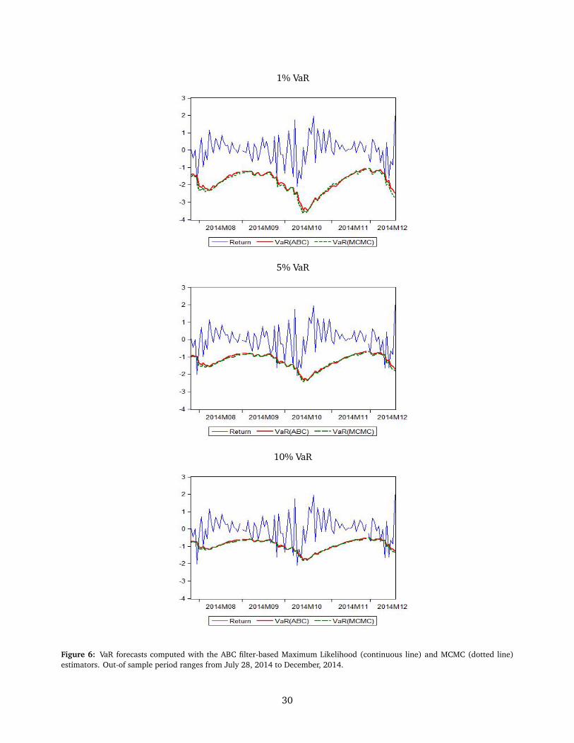
failure rate of the MCMC estimator is closer to the theoretical value. Figure 6 plots the negative

21

of the VaR forecasts computed with the two estimators for the out-of-sample period. For 5%, the

MCMC forecasts are slightly higher than those computed with the ABC filter-based ML estimator for

the last part of the out-of-sample period, but for 1% and 10% significance levels the VaR forecasts

are quite similar. This indicates that the out-of-sample performance of the model is not affected by

the in-sample estimation biases obtained when using the MCMC estimator.

6. Conclusions and further research

In this paper, we derive the statistical properties of a general family of asymmetric SV models

denoted as GASV. Some of the most popular asymmetric SV models usually implemented when

modeling heteroscedastic series with leverage effect can be included within the GASV family. In

particular, the A-ARSV model which incorporates the leverage effect through the correlation between

the standardized returns and log-volatility equations, the E-SV model which adds a noise to the

log-volatility equation specified as an EGARCH model and a restricted T-SV model, in which the

constant of the volatility equation is different depending on whether one-lagged returns are positive

or negative, are included in the GASV family. Closed-form expressions of the statistical properties

of these models are obtained when the errors are GED. We also show that the response of volatility

to positive and negative return shocks is different depending on the size and sign of the volatility

shocks.

Moreover, we analyze the finite sample properties of two estimators of the parameters. The first

is an ABC filter-based ML estimator closely related to indirect inference and the second, the MCMC

estimator implemented in the BUGS software. We show that estimating a general specification

belonging to the GASV family with the ABC filter-based ML estimator leads to accurate estimates

of the parameters even when the sample size is small. The same does not happen with the MCMC

estimator when the standardized returns follow a GED distribution. In this case, we find parameter

estimates biases. However, using BUGS reduces substantially the coding effort and the MCMC

estimator is significantly less computational and time-consuming than the ABC filter-based ML

estimator.

Finally, a general SV specification is fitted to estimate the volatilities of S&P500 daily returns.

For this particular data set, when estimating the VaRs with the two estimation methods, the failure

22

rates are similar which indicates that the out-of-sample performance of the model is not affected

by the estimation in-sample biases of the MCMC estimator.

Several possible extensions of this paper could be of interest for future research. Multivariate

asymmetric models are attracting a great deal of interest in the literature; see, for example, Harvey

et al. (1994), Asai and McAleer (2006), Chan et al. (2006), Chib et al. (2006), Jungbacker and

Koopman (2006) and Yu and Meyer (2006). Deriving the statistical properties of multivariate GASV

models is in our research agenda. Second, Rodríguez and Ruiz (2012) compare the properties

of alternative asymmetric GARCH models to see which one is closer to the empirical properties

often observed when dealing with financial returns. Comparing the properties of the GASV models

with those of the best candidates within the GARCH family is left for further research. Finally,

analyzing the behavior of the estimation procedure proposed by Skaug and Yu (2014) and the

Empirical Characteristic Function (ECF) estimator of Knight et al. (2002) in the context of the

general asymmetric SV models considered in this paper is also in our research agenda.

23

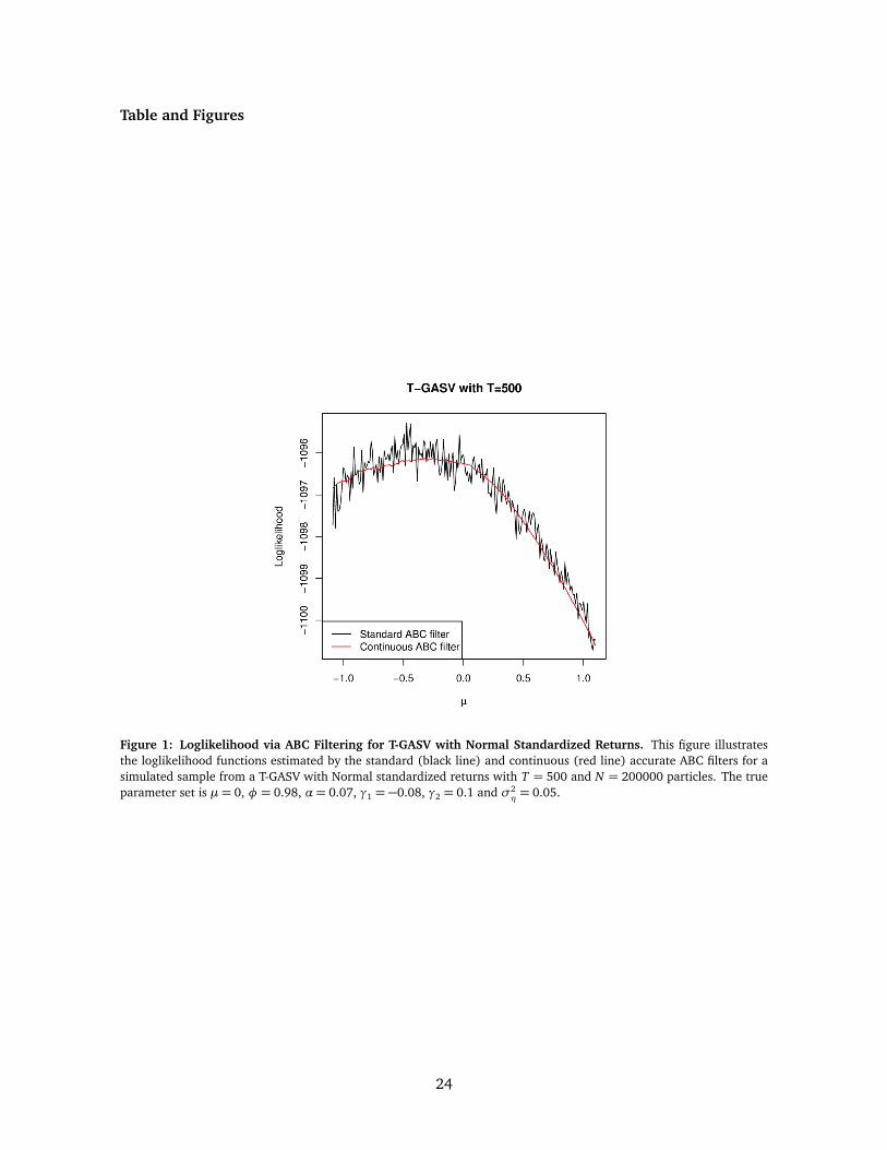
Table and Figures

Figure 1: Loglikelihood via ABC Filtering for T-GASV with Normal Standardized Returns. This figure illustratesthe loglikelihood functions estimated by the standard (black line) and continuous (red line) accurate ABC filters for asimulated sample from a T-GASV with Normal standardized returns with T = 500 and N = 200000 particles. The trueparameter set is µ= 0, φ = 0.98, α= 0.07, γ1 = −0.08, γ2 = 0.1 and σ2

η= 0.05.

24

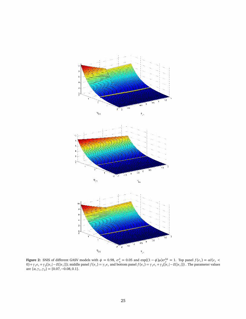
Figure 2: SNIS of different GASV models with φ = 0.98, σ2η= 0.05 and exp((1 − φ)µ)σ2φ

y = 1. Top panel f (εt) = αI(εt <

0)+γ1εt +γ2(|εt |− E(|εt |)); middle panel f (εt) = γ1εt and bottom panel f (εt) = γ1εt +γ2(|εt |− E(|εt |)) . The parameter valuesare {α,γ1,γ2}= {0.07,−0.08,0.1}.

25

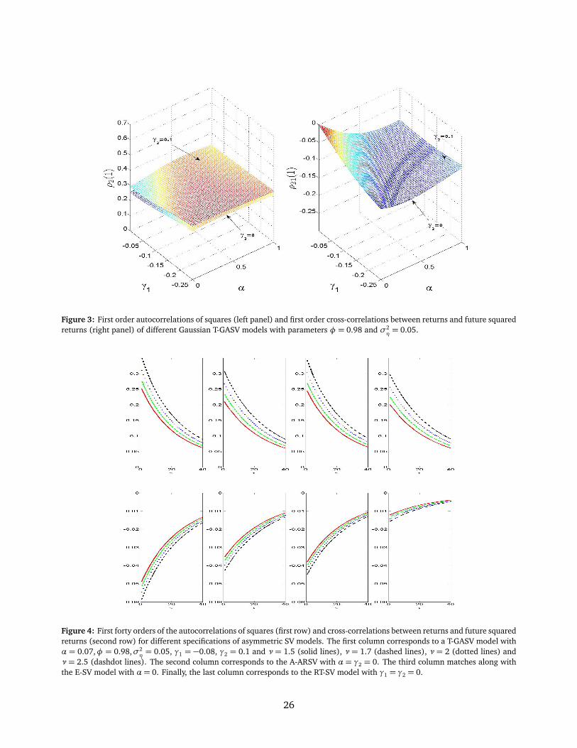
Figure 3: First order autocorrelations of squares (left panel) and first order cross-correlations between returns and future squaredreturns (right panel) of different Gaussian T-GASV models with parameters φ = 0.98 and σ2

η= 0.05.

Figure 4: First forty orders of the autocorrelations of squares (first row) and cross-correlations between returns and future squaredreturns (second row) for different specifications of asymmetric SV models. The first column corresponds to a T-GASV model withα = 0.07,φ = 0.98,σ2

η= 0.05, γ1 = −0.08, γ2 = 0.1 and ν = 1.5 (solid lines), ν = 1.7 (dashed lines), ν = 2 (dotted lines) and

ν = 2.5 (dashdot lines). The second column corresponds to the A-ARSV with α = γ2 = 0. The third column matches along withthe E-SV model with α= 0. Finally, the last column corresponds to the RT-SV model with γ1 = γ2 = 0.

26

Tabl

e1

Mon

teC

arlo

resu

lts

ofth

eA

BC

filte

r-ba

sed

Max

imum

Like

lihoo

dan

dM

CM

Ces

tim

ator

sof

the

T-G

ASV

para

met

ers.

Reg

ardi

ngth

eA

BC

esti

mat

or,v

alue

sof

the

Mon

teC

arlo

aver

ages

and

asym

ptot

icst

anda

rdde

viat

ions

(in

pare

nthe

sis)

are

repo

rted

and

for

the

MC

MC

,val

ues

ofth

eM

onte

Car

loav

erag

esan

dst

anda

rdde

viat

ions

(in

pare

nthe

sis)

ofth

epo

ster

ior

mea

nsar

ere

port

ed.

T-G

ASV

εt∼

N(0

,1)

T-G

ASV

εt∼

GE

D(0

,1)

µ·(

1−φ)

φα

γ1

γ2

σ2 η

µ·(

1−φ)

φα

γ1

γ2

σ2 η

ν

Tru

e0

0.98

0.07

-0.0

80.

10.

050

0.98

0.07

-0.0

80.

10.

051.

5

AB

C

T=50

0M

ean

0.01

20.

973

0.06

9-0

.087

0.11

10.

045

0.00

40.

975

0.07

3-0

.085

0.11

50.

045

1.50

1St

d.de

v.(0

.044

)(0

.015

)(0

.076

)(0

.053

)(0

.103

)(0

.024

)(0

.032

)(0

.010

)(0

.057

)(0

.046

)(0

.095

)(0

.025

)(0

.127

)

T=10

00M

ean

0.00

40.

977

0.07

2-0

.082

0.10

70.

048

0.00

10.

978

0.07

2-0

.081

0.10

80.

047

1.49

5St

d.de

v.(0

.023

)(0

.008

)(0

.042

)(0

.030

)(0

.074

)(0

.016

)(0

.017

)(0

.006

)(0

.028

)(0

.029

)(0

.070

)(0

.016

)(0

.081

)

T=20

00M

ean

0.00

20.

978

0.07

1-0

.082

0.09

80.

049

0.00

20.

979

0.06

9-0

.083

0.10

10.

049

1.49

2St

d.de

v.(0

.013

)(0

.005

)(0

.021

)(0

.020

)(0

.052

)(0

.011

)(0

.011

)(0

.004

)(0

.017

)(0

.020

)(0

.055

)(0

.013

)(0

.066

)

MC

MC

T=50

0M

ean

0.01

50.

965

0.09

6-0

.074

0.14

50.

041

0.01

40.

961

0.09

5-0

.075

0.18

40.

024

1.46

2St

d.de

v.(0

.065

)(0

.019

)(0

.113

)(0

.061

)(0

.168

)(0

.026

)(0

.062

)(0

.023

)(0

.110

)(0

.064

)(0

.234

)(0

.018

)(0

.323

)

T=10

00M

ean

0.00

40.

974

0.08

3-0

.077

0.13

90.

045

0.00

20.

973

0.08

2-0

.077

0.18

10.

027

1.42

7St

d.de

v.(0

.040

)(0

.010

)(0

.076

)(0

.040

)(0

.106

)(0

.019

)(0

.040

)(0

.011

)(0

.076

)(0

.042

)(0

.181

)(0

.017

)(0

.216

)

T=20

00M

ean

0.00

00.

977

0.07

8-0

.078

0.11

90.

048

0.00

00.

973

0.08

6-0

.074

0.21

00.

023

1.39

0St

d.de

v.(0

.029

)(0

.006

)(0

.055

)(0

.028

)(0

.064

)(0

.011

)(0

.040

)(0

.011

)(0

.078

)(0

.044

)(0

.152

)(0

.016

)(0

.209

)

27

Tabl

e2

Para

met

eres

tim

ates

(lef

tpa

nel)

ofth

eT-

GA

SVm

odel

usin

gS&

P50

0re

turn

sbe

twee

nSe

ptem

ber

9,19

98an

dJu

ly25

,201

4,an

dfa

ilure

rate

sof

the

1%,5

%an

d10

%Va

Rfo

reca

sts

for

the

out-

of-s

ampl

epe

riod

July

28,2

014

-Dec

embe

r17

2014

.St

anda

rder

rors

ofpa

ram

eter

esti

mat

esar

ere

port

edin

pare

nthe

ses.

Reg

ardi

ngth

eA

BC

esti

mat

or,

asym

ptot

icst

anda

rder

rors

are

repo

rted

and

for

the

MC

MC

,po

ster

ior

stan

dard

erro

rsar

ere

port

ed.

AB

C-fi

lter

esti

mat

edlo

glik

elih

oods

are

also

repo

rted

.H

eter

oske

dast

icit

yan

dau

toco

rrel

atio

nco

nsis

tent

Vuon

gte

stco

mpa

ring

the

MC

MC

spec

ifica

tion

toth

eA

BC

filte

red

spec

ifica

tion

are

repo

rted

inpa

rent

hesi

sbe

low

the

log-

likel

ihoo

dva

lue

ofth

eM

CM

Clo

glik

elih

ood.

AB

CLo

g-Li

kelih

ood

VaR

fore

cast

sµ·(

1−φ)

φα

γ1

γ2

σ2 η

ν1%

5%10

%

AB

C-0

.047

80.

9814

0.14

42-0

.106

40.

0254

0.00

771.

6828

-571

7.03

0.02

970.

0693

0.11

88(0

.003

6)(0

.001

7)(0

.008

2)(0

.009

3)(0

.014

6)(0

.000

9)(0

.043

5)(0

.017

0)(0

.025

4)(0

.032

4)

MC

MC

0.00

010.

9795

0.00

62-0

.146

50.

0717

0.00

581.

5315

-572

1.96

0.02

970.

0594

0.11

88(0

.016

2)(0

.003

7)(0

.029

1)(0

.017

4)(0

.044

2)(0

.002

9)(0

.139

7)(0

.032

9)(0

.017

0)(0

.023

6)(0

.032

4)

28

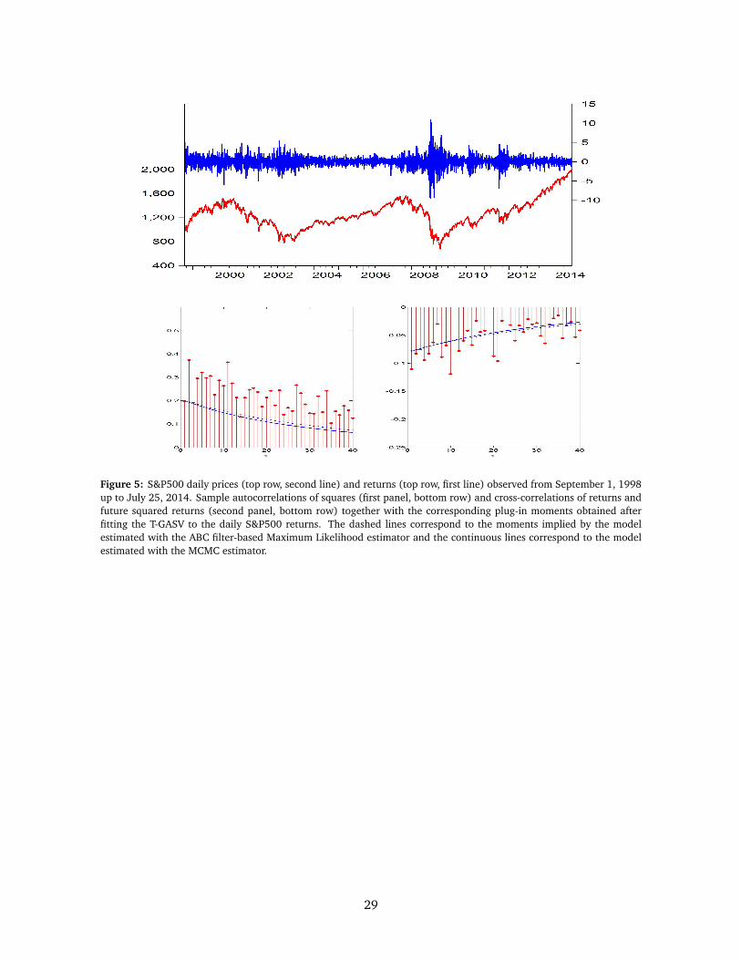
Figure 5: S&P500 daily prices (top row, second line) and returns (top row, first line) observed from September 1, 1998up to July 25, 2014. Sample autocorrelations of squares (first panel, bottom row) and cross-correlations of returns andfuture squared returns (second panel, bottom row) together with the corresponding plug-in moments obtained afterfitting the T-GASV to the daily S&P500 returns. The dashed lines correspond to the moments implied by the modelestimated with the ABC filter-based Maximum Likelihood estimator and the continuous lines correspond to the modelestimated with the MCMC estimator.

29

1% VaR

5% VaR

10% VaR

Figure 6: VaR forecasts computed with the ABC filter-based Maximum Likelihood (continuous line) and MCMC (dotted line)estimators. Out-of sample period ranges from July 28, 2014 to December, 2014.

30

Appendix A. Proof of Theorems

Appendix A.1. Proof of Theorem 2.1

Consider yt , which, according to equation (1), is given by yt = εt exp (ht/2). From equation

(2), ht can be written as

ht −µ=∞∑

i=1

φ i−1( f (εt−i) +ηt−i). (A.1)

First, note that if |φ|< 1 and x = (x1, x2, · · · ) ∈ R∞, then Ψ(x) =∑∞

i=1φi−1 x i is a measurable

function. Given that for any x0 and ∀ς > 0, we can find a value of δ =p

1−φ2ς, such that ∀x

satisfying |x − x0|=q

∑∞i=1(x i − x0

i )2 < δ, we have |Ψ(x)−Ψ(x0)|= |

∑∞i=1φ

i−1(x i − x0i )|. Using

the Cauchy-Schwarz inequality, it follows that |Ψ(x)−Ψ(x0)| ≤q

∑∞i=1φ

2i−2q

∑∞i=1(x i − x0

i )2 <

δp1−φ2

= ς. Therefore, Ψ(x) is continuous, and consequently, measurable.

Second, given that εt and ηt are both IID and mutually independent for any lag and lead, then

{ f (εt)+ηt} is also an IID sequence. Lemma 3.5.8 of William (1974) states that an IID sequence is

always strictly stationary. Therefore, in (A.1), if |φ| < 1, ht is expressed as a measurable function

of a strictly stationary process and, consequently, according to Theorem 3.5.8 of William (1974),

ht is strictly stationary. As σt is a continuous function of ht , σt is also strictly stationary. The level

noise εt is independent of σt and strictly stationary by definition. Therefore, it is easy to show that

yt = σtεt is strictly stationary.

When |φ| < 1, yt and σ2t are strictly stationary and, consequently, any existing moments are

time invariant. Next we show that σt has finite moments of arbitrary positive order c when εt

follows a distribution such that E(exp(0.5c f (εt)))<∞.

From expression (A.1), the power-transformed volatility can be written as follows

σct = exp(0.5cµ)exp

�

0.5c∞∑

i=1

φ i−1( f (εt−i) +ηt−i)

�

. (A.2)

Given that εt and ηt are mutually independent for all lags and leads, the following expression is

obtained after taking expectations on both sides of equation (A.6)

E(σct) = exp(0.5cµ)E

�

exp

�

0.5c∞∑

i=1

φ i−1 f (εt−i)

��

E

�

exp

�

0.5c∞∑

i=1

φ i−1ηt−i

��

. (A.3)

31

Asηt is Gaussian, the last expectation in (A.3) can be evaluated using the expression of the moments

of the Log-Normal. Furthermore, given that ηt and εt are both IID sequences, it is easy to show

that (A.3) becomes

E(σct ) = exp(0.5cµ)exp

�

c2σ2η

8 (1−φ2)

� ∞∏

i=1

E�

exp�

0.5cφ i−1 f (εt−i)��

. (A.4)

We need to show that P(0.5c,φ)≡∞∏

i=1

E�

exp�

0.5cφ i−1 f (εt−i)��

is finite when E (exp (0.5c f (εt−i))])<

∞. In general, we are going to prove that when∑∞

i=1 |bi|<∞ and E(exp(bi f (εt−i)))<∞, then∞∏

i=1

E [exp (bi f (εt−i))] is always finite.

Define ai = E(exp(bi f (εt−i))). As 0 < ai < ∞, according to Section 0.25 of Ryzhik et al.

(2007), the sufficient and necessary condition for the infinite product∏∞

i=1 ai to converge to a

finite, nonzero number is that the series∑∞

i=1(ai − 1) converge. Expanding ai in Taylor series

around bi = 0, we have

ai − 1= O(bi) as bi → 0.

Consequently, for some ς > 0, there exist a finite M independent of i such that

sup|bi |<ς,bi 6=0

|O(bi)|< M |bi|.

∑∞i=1 |bi|<∞ implies

∑∞i=1 |ai − 1|<∞, therefore

∑∞i=1(ai − 1)<∞. Thus

∏∞i=1 ai <∞.

Here bi = 0.5cφ i−1. Therefore, if |φ| < 1, then∑∞

i=1 |bi| =0.5c1−φ <∞. Thus, the product

∏∞i=1 E(exp(0.5cφ i−1 f (εt−i))) and, consequently, E(σc

t ) are finite when E(exp(0.5cφ i−1 f (εt−i)))<

∞. Note that when |φ| < 1, E(exp(0.5c f (εt))) <∞ guarantees that E(exp(0.5cφ i−1 f (εt−i))) <

∞ for any positive integer i. Therefore, if |φ|< 1 and E(exp(0.5c f (εt)))<∞, E(σct) is finite.

Finally, consider yt , which, according to equation (1), is given by yt = σtεt . Therefore, given

that σt and εt are contemporaneously independent, the following expressions are obtained

E(|yt |c) = E(σct)E(|εt |c), (A.5)

E(y ct ) = E(σc

t)E(εct). (A.6)

32

Replacing formula (A.4) into (A.5) yields the following required expression

E (|yt |c) = exp(0.5cµ)E (|εt |c)exp

�

c2σ2η

8 (1−φ2)

�

P(0.5c,φ)), (A.7)

where P(x , y) ≡∏∞

i=1 E(exp(x y i−1 f (εt−i))). Therefore, if further εt follows a distribution such

that E(εct) <∞, which is equivalent to E(|εt |c) <∞, then |yt | has finite moments of arbitrary

order c. On the other hand, following the same steps, we obtain

E�

y ct

�

= exp(0.5cµ)E�

εct

�

exp

�

c2σ2η

8 (1−φ2)

�

P(0.5c,φ)). (A.8)

Thus, E(y ct )<∞ if |φ|< 1, E(εc

t)<∞ and E(exp(0.5c f (εt)))<∞.

Appendix A.2. Proof of Theorem 2.2

Consider yt as given in equations (1) and (2). We first compute the τ-th order auto-covariance

of |yt |c which is given by

E(|εt |cσct |εt−τ|cσc

t−τ)− [E(|yt |c)]2. (A.9)

Note that from equation (2), σct = exp {0.5cht} can be written as follows

σct = exp {0.5cµ(1−φτ)}exp

¨

0.5cτ∑

i=1

φ i−1( f (εt−i) +ηt−i)

«

σcφτ

t−τ. (A.10)

The following expression of the auto-covariance is obtained after substituting (A.7) and (A.10) into

(A.9)

cov(|yt |c , |yt−τ|c) =

E

�

|εt |c|εt−τ|c exp(0.5cµ(1−φτ))exp

�

τ∑

i=1

0.5cφ i−1( f (εt−i) +ηt−i)

�

σc(φτ+1)t−τ

�

−

¨

exp(0.5cµ)E (|εt |c)exp

�

c2σ2η

8 (1−φ2)

�

P(0.5c,φ))

«2

. (A.11)

Given that εt and ηt are IID sequences mutually independent for any lag and lead and thatσt−τ only depends on lagged disturbances, substituting the time-invariant moment of σt in (A.4),

33

equation (A.11) can be written as follows

cov(|yt |c , |yt−τ|c) =

exp(cµ)E (|εt |c)exp�

1+φτ

4 (1−φ2)c2σ2

η

�

E�

|εt |c exp�

0.5cφτ−1 f (εt)��

τ−1∏

i=1

E�

exp�

0.5cφ i−1 f (εt−i)��

·∞∏

i=1

E�

exp�

0.5c (1+φτ)φ i−1 f (εt−i)��

− exp(cµ)(E(|εt |c))2 exp

�

c2σ2η

4 (1−φ2)

�

[P(0.5c,φ)]2.

The required expression of ρc(τ) follows directly from ρc(τ) =cov(|yt |c ,|yt−τ|c)

E(|yt |2c)−[E(|yt |c)]2, where the

denominator can be obtained from (A.7).

Appendix A.3. Proof of Theorem 2.3The calculation of the cross-covariance between |yt |c and yt−τ is obtained following the same

steps as in Appendix A.2. That is

cov (|yt |c , yt−τ) = exp(0.5(c + 1)µ)E (|εt |c)exp

�

1+ c2 + 2cφτ

8 (1−φ2)σ2η

�

E�

εt exp�

0.5cφτ−1 f (εt)��

·∞∏

i=1

E�

exp�

0.5 (1+ cφτ)φ i−1 f (εt−i)��

τ−1∏

i=1

E�

exp�

0.5cφ i−1 f (εt−i)��

. (A.12)

Finally, ρc1(τ) =cov(|yt |c ,yt−τ)p

E(|yt |2c)−E2(|yt |c)Æ

E(y2t )

together with (A.7) and (A.12) yields the required equation

(8).

Appendix B. Expectations

Appendix B.1. Expectations needed to compute E(|yt |c), cor r(|yt |c , |yt+τ|c) and cor r(yt , |yt+τ|c)when ε∼ GED(ν) and f (ε) = αI(ε < 0) + γ1ε+ γ2(|ε| − E|ε|)

If ε has a centered and standardized GED distribution, with parameter 0 < ν ≤ ∞, then,

the density function of ε is given by ψ(ε) = C0 exp�

− |ε|ν

2λν

�

, where C0 ≡ν

λ21+1/νΓ (1/ν) and λ ≡�

2−2/νΓ (1/ν)/Γ (3/ν)�1/2

, with Γ (·) being the Gamma function. Thus, given that the distribution

of ε is symmetric with support (−∞,∞), if p is a nonnegative finite integer, then

E(|ε|p) = C0

∫ +∞

−∞|ε|p exp

�

−|ε|ν

2λν

�

dε

= 2C0

∫ +∞

0

εp exp�

−εν

2λν

�

dε.

Substituting s = εν

2λν and solving the integral yields

E(|ε|p) = 2pνλpΓ ((p+ 1)/ν)/Γ (1/ν) . (B.1)

34

On the other hand,

E(|ε|p exp(b f (ε)))

=

∫ +∞

−∞|ε|p exp(bαI(ε < 0) + bγ1ε+ bγ2(|ε| − E|ε|))C0 exp

�

−|ε|ν

2λν

�

dε

= C0 exp(−bγ2E|ε|)

�

∫ 0

−∞(−ε)p exp(bα)exp(b(γ1 − γ2)ε)exp

�

−(−ε)ν

2λν

�

dε

+

∫ +∞

0

εp exp(b(γ1 + γ2)ε)exp�

−εν

2λν

�

dε

�

.

Integrating by substitution with s = −ε in the first integral, we obtain

E(|ε|p exp(b f (ε))) = C0 exp(−bγ2E|ε|)�∫ +∞

0

sp exp(bα)exp(b(γ2 − γ1)s)exp�

−sν

2λν

�

ds

+

∫ +∞

0

εp exp(b(γ1 + γ2)ε)exp�

−εν

2λν

�

dε

�

(B.2)

= C0 exp(−bγ2E|ε|)∫ +∞

0

εp exp�

−εν

2λν

�

[exp(bα)exp(b(γ2 − γ1)ε) + exp(b(γ1 + γ2)ε)] dε.

We can rewrite the previous equation by replacing ε with λ(2y)1/ν as follows

E(|ε|p exp(b f (ε)))

= C0 exp(−bγ2E|ε|)λp+12

1+pν

ν

·∫ +∞

0

y−1+ 1+pν exp(−y)

�

exp(bα)exp(b(γ2 − γ1)λ21ν y

1ν ) + exp(b(γ1 + γ2)λ2

1ν y

1ν )�

d y.

Expanding the expression within the square brackets in a Taylor series and substituting C0, thefollowing expression is obtained

E(|ε|p exp(b f (ε)))

= exp�

−bγ221νλΓ (2/ν)/Γ (1/ν)

� λp2pν−1

Γ�

1ν

�

·∫ +∞

0

+∞∑

k=0

h

exp(bα)�

bλ21ν (γ2 − γ1)

�k+�

bλ21ν (γ1 + γ2)

�ki y−1+ 1+p+kν exp(−y)

k!d y. (B.3)

Define∆= max�

|bλ21/ν(γ1 + γ2)|, max(exp(bα), 1)|bλ21/ν(γ2 − γ1)|

. Then, we can use the

results in Nelson (1991) to show that if ν > 1 then the summation and integration in (B.3) can

be interchanged. Further, applying Formula 3.381 #4 of Ryzhik et al. (2007) yields the following

35

required expression20

E(|ε|p exp(b f (ε)))

= exp�

−bγ221/νλΓ (2/ν)/Γ (1/ν)�

2p/νλp∞∑

k=0

(21/νλb)k�

(γ1 + γ2)k + exp(bα)(γ2 − γ1)

k� Γ ((p+ k+ 1)/ν)

2Γ (1/ν)k!<∞.

(B.4)

Following the same steps, the following required expression is obtained when ν > 1,

E(εp exp(b f (ε)))

= exp�

−bγ221/νλΓ (2/ν)/Γ (1/ν)�

2p/νλp

·∞∑

k=0

(21/νλb)k�

(γ1 + γ2)k + (−1)p exp(bα)(γ2 − γ1)

k� Γ ((p+ k+ 1)/ν)

2Γ (1/ν)k!<∞. (B.5)

Note that the expectations (B.4) and (B.5) are only valid when ν > 1. When 0< ν≤ 1, it is not

possible to obtain closed-form expression of the required expectations. In this case, we can only

obtain the conditions for the expectations to be finite. When 0 < ν < 1, it is very easy to verify

that E(|ε|p exp(b f (ε)))<∞ if and only if the both integrals in (B.2) are finite, which holds if and

only if b(γ2 − γ1) ≤ 0 and b(γ2 + γ1) ≤ 0. When ν = 1, similarly, the sufficient and necessary

conditions for the infinity of E(|ε|p exp(b f (ε))) are b(γ2 − γ1) <1

2λ and b(γ2 + γ1) <1

2λ . That is

b(γ2 − γ1) <p

2 and b(γ2 + γ1) <p

2. The conditions for the infinity of E(εp exp(b f (ε))) are the

same as those for E(|ε|p exp(b f (ε))) 0< ν≤ 1.

Finally, when ε ∼Student-t with d degrees of freedom (d > 2) and is normalized to satisfy

E(ε) = 0, var(ε) = 1, then

E(|ε|p exp(b f (ε)))

= C1

∫ +∞

0

εp exp(bα)exp(b(γ2 − γ1)ε)

�

1+ε2

d − 2

�− d+12

dε

+

∫ +∞

0

εp exp(b(γ1 + γ2)ε)

�

1+ε2

d − 2

�− d+12

dε, (B.6)

20See Nelson (1991) for the proof of finiteness of the formula.

36

where C1 =Γ( d+1

2 )p(d−2)πΓ( d

2 )exp

�

−bγ221/νλΓ (2/ν)/Γ (1/ν)�

. We can verify that E(|ε|p exp(b f (ε))) =

∞ unless b(γ2 − γ1)≤ 0 and b(γ2 + γ1)≤ 0.

Appendix B.2. Expectations needed to compute E(|yt |c), cor r(|yt |c , |yt+τ|c) and cor r(yt , |yt+τ|c)when ε∼ N(0,1)

Assume that all the parameters are defined as in equations (1) and (2). When ε∼ N(0,1), using

the expression (B.2) and the formula 3.462-1 of Ryzhik et al. (2007), the following expressions for

any positive integer p and any integer b are derived

E(|ε|p exp(b f (ε))) =1p

2πexp

�

−bγ2

√

√ 2π

�

�

exp(bα)Γ (p+ 1)exp

�

b2(γ1 − γ2)2

4

�

D−p−1(b(γ1 − γ2))

+Γ (p+ 1)exp

�

b2(γ1 + γ2)2

4

�

D−p−1(−b(γ1 + γ2))

�

(B.7)

and

E(εp exp(b f (ε))) =1p

2πexp

�

−bγ2

√

√ 2π

�

�

(−1)p exp(bα)Γ (p+ 1)exp

�

b2(γ1 − γ2)2

4

�

D−p−1(b(γ1 − γ2))

+Γ (p+ 1)exp

�

b2(γ1 + γ2)2

4

�

D−p−1(−b(γ1 + γ2))

�

, (B.8)

where D−a(·) is the parabolic cylinder function. Particularly, when p = 0,1 or 2, the expressions

are reduced to

E(exp(b f (ε))) = exp

�

−bγ2

√

√ 2π

�

�

exp(bα)exp�

A�

Φ(C) + exp�

B�

Φ(D)�

,

E(εexp(b f (ε))) =1p

2πexp

�

−bγ2

√

√ 2π

�

�

−exp(bα)�

1+p

2πC exp(A)Φ(C)�

+�

1+p

2πD exp(B)Φ(D)�

,

E(|ε|exp(b f (ε))) =1p

2πexp

�

−bγ2

√

√ 2π

�

�

exp(bα)�

1+p

2πC exp(A)Φ(C)�

+�

1+p

2πD exp(B)Φ(D)�

and

E(|ε|2 exp(b f (ε))) =1p

2πexp

�

−bγ2

√

√ 2π

�

·�

exp(bα)�

C +p

2π(C2 + 1)exp(A)Φ(C)�

+�

D+p

2π(D2 + 1)exp(B)Φ(D)�

,

37

where Φ(·) is the Normal distribution function, A= b2(γ1−γ2)2

2 , B = b2(γ1+γ2)2

2 , C = −b(γ1 − γ2) and

D = b(γ1 + γ2).

Appendix C. Continuous Resampling of {x (n)t ,1 } using Malik and Pitt (2011) procedure

Step (i) (Sorting): Sort the particles { x (n)t,1} in ascending order

x (1)t,1 ≤ x (2)t,1 ≤ · · · ≤ x (N)t,1 .

Denote the importance weight associated with x (n)t,1 by p(n)t .

Step (ii) (Sorted uniforms): Draw sorted {ui} using Malmquist (1950)’s sorted uniforms. That is draw

{vi} from a uniform distribution on the interval (0,1). Set uN = v1/NN and for n= N−1, . . . , 1:

un = un+1v1/nn , .

The resulting u1 < u2 < · · ·< uN are ordered uniform variables.

Step (iii) (Index sampling): Define π(0)t = p(1)t /2, π(N)t = p(N)t /2 and π(k)t = (p(k+1)t + p(k)t )/2 for

k = 1, . . . , N − 1, and set s = 0, j = 1. For i = 0, . . . , N , sample indexes r1, . . . , rN and a new

set of uniforms u∗1, . . . , u∗N :

s = s+π(i)t

while (u j ≤ s AND j ≤ N) {

r j = i

u∗j = (u j − (s−π(i)t ))/π

(i)t

j = j + 1

}

Step (iv) (Particle drawing): For the selected regions where r j = 0, we set x ( j)t,1 = x (1)t,1 and where

r j = N we set x ( j)t,1 = x (N)t,1 . Otherwise, set

x ( j)t,1 = ( x(r j+1)t,1 − x

(r j)t,1 )× u∗j + x

(r j)t,1 .

38

Abanto-Valle, C.A., Bandyopadhyay, D., Lachos, V.H., Enriquez, I., 2010. Robust Bayesian

analysis of heavy-tailed stochastic volatility models using scale mixtures of normal distributions.

Computational Statistics & Data Analysis 54, 2883–2898.

Andersen, T.G., Bollerslev, T., Diebold, F., Labys, P., 2001a. The distribution of realized exchange

rate volatility. Journal of the American Statistical Association 96, 42–55.

Andersen, T.G., Bollerslev, T., Diebold, F.X., Ebens, H., 2001b. The distribution of realized stock

return volatility. Journal of Financial Economics 61, 43–76.

Andersen, T.G., Bollerslev, T., Diebold, F.X., Labys, P., 2003. Modeling and forecasting realized

volatility. Econometrica 71, 579–625.

Asai, M., 2005. Comparison of MCMC methods for estimating stochastic volatility models.

Computational Economics 25, 281–301.

Asai, M., 2008. Autoregressive stochastic volatility models with heavy-tailed distributions: A

comparison with multifactor volatility models. Journal of Empirical Finance 15, 332–341.

Asai, M., McAleer, M., 2005. Dynamic asymmetric leverage in stochastic volatility models.

Econometric Reviews 24, 317–332.

Asai, M., McAleer, M., 2006. Asymmetric multivariate stochastic volatility. Econometric Reviews

25, 453–473.

Asai, M., McAleer, M., 2011. Alternative asymmetric stochastic volatility models. Econometric

Reviews 30, 548–564.

Asai, M., McAleer, M., Medeiros, M.C., 2012. Asymmetry and long memory in volatility modeling.

Journal of Financial Econometrics 10, 495–512.

Bartolucci, F., De Luca, G., 2003. Likelihood-based inference for asymmetric stochastic volatility

models. Computational Statistics & Data Analysis 42, 445–449.

Bauwens, L., Rombouts, J.V.K., 2004. Econometrics. SpringerVerlag: New York. pp. 951–979.

39

Breidt, F.J., 1996. A threshold autoregressive stochastic volatility model, in: VI Latin American

Congress of Probability and Mathematical Statistics (CLAPEM), Valparaiso, Chile, Citeseer.

Broto, C., Ruiz, E., 2004. Estimation methods for stochastic volatility models: A survey. Journal of

Economic Surveys 18, 613–649.

Calvet, L., Czellar, V., 2011. State-observation sampling and the econometrics of learning models.

Technical report, arXiv:1105.4519 .

Calvet, L., Czellar, V., 2014. Accurate methods for approximate bayesian computation filtering.

Journal of Financial Econometrics, forthcoming .

Cappuccio, N., Lubian, D., Raggi, D., 2004. MCMC Bayesian estimation of a skew-GED stochastic

volatility model. Studies in Nonlinear Dynamics & Econometrics 8.

Carnero, M.A., Peña, D., Ruiz, E., 2004. Persistence and kurtosis in GARCH and stochastic volatility

models. Journal of Financial Econometrics 2, 319–342.

Chan, D., Kohn, R., Kirby, C., 2006. Multivariate stochastic volatility models with correlated errors.

Econometric Reviews 25, 245–274.

Chen, C.W.S., Liu, F.C., So, M.K.P., 2008. Heavy-tailed-distributed threshold stochastic volatility

models in financial time series. Australian & New Zealand Journal of Statistics 50, 29–51.

Chib, S., 2001. Markov chain Monte Carlo methods: Computation and inference. North-Holland,

Amsterdam. volume 5. pp. 3569–3649.

Chib, S., Nardari, F., Shephard, N., 2002. Markov chain Monte Carlo methods for stochastic

volatility models. Journal of Econometrics 108, 281–316.

Chib, S., Nardari, F., Shephard, N., 2006. Analysis of high dimensional multivariate stochastic

volatility models. Journal of Econometrics 134, 341–371.

Choy, B., Wai, Y., Chan, C., 2008. Bayesian Student-t stochastic volatility models via scale mixtures.

Advances in Econometrics 23, 595–618.

40

Demos, A., 2002. Moments and dynamic structure of a time-varying parameter stochastic volatility

in mean model. Econometrics Journal 5, 345–357.

Dhaene, G., 2004. Indirect inference for stochastic volatility models via the log-squared

observations. Review of Business and Economics XLIX, 421–440.

Durham, G.B., 2006. Monte Carlo methods for estimating, smoothing, and filtering one-and

two-factor stochastic volatility models. Journal of Econometrics 133, 273–305.

Durham, G.B., 2007. SV mixture models with application to S&P500 index returns. Journal of

Financial Economics 85, 822–856.

Engle, R., Ng, V., 1993. Measuring and testing the impact of news on volatility. The Journal of

Finance 48, 1779–1801.

Ghysels, E., Harvey, A., Renault, E., 1996. Stochastic Volatility. Amsterdam: North-Holland.

Gordon, N., Salmon, D., Smith, A.F., 1993. Novel approach to nonlinear/non-gaussian bayesian

state estimation. IEE Proceedings F 140, 107–113.

Gourieroux, C., Monfort, A., Renault, E., 1993. Indirect inference. Journal of Applied Econometrics

8, S85–S118.

Harvey, A., Ruiz, E., Shephard, N., 1994. Multivariate stochastic variance models. The Review of

Economic Studies 61, 247–264.

Harvey, A.C., 1990. The Econometric Analysis of Time Series. Cambridge: MIT Press. Second

edition.

Harvey, A.C., Shephard, N., 1996. Estimation of an asymmetric stochastic volatility model for asset

returns. Journal of Business & Economic Statistics 14, 429–34.

Huang, S.J., Yu, J., 2008. An efficient method for maximum likelihood estimation of a stochastic

volatility model. Statistics and its Interface 1, 289–296.

Jacquier, E., Polson, N.G., Rossi, P.E., 1994. Bayesian analysis of stochastic volatility models: Reply.

Journal of Business & Economic Statistics 12, 413–417.

41

Jasra, A., Singh, S., Martin, J., McCoy, E., 2012. Filtering via Approximate Bayesian Computation.

Statistics and Computing 22, 1223–1237.

Jungbacker, B., Koopman, S.J., 2006. Monte Carlo likelihood estimation for three multivariate

stochastic volatility models. Econometric Reviews 25, 385–408.

Jungbacker, B., Koopman, S.J., 2007. Monte Carlo estimation for nonlinear non-Gaussian state

space models. Biometrika 94, 827–839.

Kim, S., Shephard, N., Chib, S., 1998. Stochastic volatility: Likelihood inference and comparison

with ARCH models. The Review of Economic Studies 65, 361–393.

Knight, J.L., Satchell, S.E., Yu, J., 2002. Estimation of the stochastic volatility model by the

empirical characteristic function method. Australian & New Zealand Journal of Statistics ,

319–335.

Koopman, S.J., Shephard, N., Creal, D., 2009. Testing the assumptions behind importance

sampling. Journal of Econometrics 149, 2–11.

Liesenfeld, R., Jung, R.C., 2000. Stochastic volatility models: conditional normality versus

heavy-tailed distributions. Journal of Applied Econometrics 15, 137–160.

Liesenfeld, R., Richard, J.F., 2003. Univariate and multivariate stochastic volatility models:

Estimation and diagnostics. Journal of Empirical Finance 10, 505–531.

Liesenfeld, R., Richard, J.F., 2006. Classical and Bayesian analysis of univariate and multivariate

stochastic volatility models. Econometric Reviews 25, 335–360.

Maheu, J.M., McCurdy, T.H., 2004. News arrival, jump dynamics, and volatility components for

individual stock returns. The Journal of Finance 59, 755–793.

Malik, S., Pitt, M.K., 2011. Particle filters for continuous likelihood evaluation and maximisation.

Journal of Econometrics 165, 190–209.

Malmquist, S., 1950. On a property of order statitics from a rectangular distribution. Skand.

Aktuarietidskr 33, 214–222.

42

Mao, X., Ruiz, E., Veiga, H., 2013. One for all: Nesting asymmetric stochastic volatility models

WP131110, Universidad Carlos III de Madrid.

McAleer, M., 2005. Automated inference and learning in modeling financial volatility. Econometric

Theory 21, 232–261.

Melino, A., Turnbull, S.M., 1990. Pricing foreign currency options with stochastic volatility. Journal

of Econometrics 45, 239–265.

Meyer, R., Yu, J., 2000. BUGS for a Bayesian analysis of stochastic volatility models. The

Econometrics Journal 3, 198–215.

Monfardini, C., 1998. Estimating stochastic volatility models through indirect inference. The

Econometrics Journal 1, 113–128.

Nakajima, J., Omori, Y., 2009. Leverage, heavy-tails and correlated jumps in stochastic volatility

models. Computational Statistics & Data Analysis 53, 2335–2353.

Nakajima, J., Omori, Y., 2012. Stochastic volatility model with leverage and asymmetrically

heavy-tailed error using GH skew Studentars t-distribution. Computational Statistics & Data

Analysis 56, 3690–3704.

Nelson, D., 1991. Conditional heteroscedasticity in asset pricing: A new approach. Econometrica

59, 347–370.

Omori, Y., Chib, S., Shephard, N., Nakajima, J., 2007. Stochastic volatility with leverage: Fast and

efficient likelihood inference. Journal of Econometrics 140, 425–449.

Omori, Y., Watanabe, T., 2008. Block sampler and posterior mode estimation for asymmetric

stochastic volatility models. Computational Statistics & Data Analysis 52, 2892–2910.

Pérez, A., Ruiz, E., Veiga, H., 2009. A note on the properties of power-transformed returns in

long-memory stochastic volatility models with leverage effect. Computational Statistics & Data

Analysis 53, 3593–3600.

43

Rodríguez, M.J., Ruiz, E., 2012. GARCH models with leverage effect: differences and similarities.

Journal of Financial Econometrics 10(4), 637–668.

Ruiz, E., 1994. Quasi-maximum likelihood estimation of stochastic volatility models. Journal of

Econometrics 63, 289–306.

Ruiz, E., Veiga, H., 2008a. Modelling long-memory volatilities with leverage effect: A-LMSV versus

FIEGARCH. Computational Statistics & Data Analysis 52, 2846–2862.

Ruiz, E., Veiga, H., 2008b. Modelos de la volatilidad estocástica: Una alternativa atractiva y factible

para modelizar la evolución de la volatidad. Anales de Estudios Economicos y Empresariales

XVIII, 9–68.

Ryzhik, I.M., Jeffrey, A., Zwillinger, D., 2007. Table of integrals, series and products. London:

Academic Press. Seventh edition.

Sandmann, G., Koopman, S.J., 1998. Estimation of stochastic volatility models via Monte Carlo

maximum likelihood. Journal of Econometrics 87, 271–301.

Shephard, N.G., 1996. Statistical aspects of ARCH and stochastic volatility. Chapman and Hall,

London. pp. 1–67.

Shephard, N.G., 2005. Stochastic Volatility: Selected Readings. Oxford University Press, Oxford.

Skaug, H.J., Yu, J., 2014. A flexible and automated likelihood based framework for inference in

stochastic volatility models. Computational Statistics and Data Analysis 76, 642–654.

So, M.K.P., Li, W.K., Lam, K., 2002. A threshold stochastic volatility model. Journal of Forecasting

21, 473–500.

Takahashi, M., Omori, Y., Watanabe, T., 2013. News impact curve for stochastic volatility models.

Economics Letters 120, 130–134.

Taylor, S.J., 1982. Financial returns modelled by the product of two stochastic processes-a study

of the daily sugar prices 1961-75. North-Holland, Amsterdam. volume 1. pp. 203–206.

44

Taylor, S.J., 1986. Modelling Financial Time Series. Chichester: Wiley.

Taylor, S.J., 1994. Modelling stochastic volatility: A review and comparative study. Mathematical

Finance 4, 183–204.

Taylor, S.J., 2007. Asset price dynamics, volatility, and prediction. Princeton, NJ: Princeton

University Press.

Tsiotas, G., 2012. On generalised asymmetric stochastic volatility models. Computational Statistics

& Data Analysis 56, 151–172.

Walker, S.G., Gutiérrez-Peña, E., 1999. Robustifying Bayesian procedures. Bayesian Statistics 6,

685–710.

Wang, J.J.J., Chan, J.S.K., Boris Choy, S.T., 2011. Stochastic volatility models with leverage and

heavy-tailed distributions: A Bayesian approach using scale mixtures. Computational Statistics

& Data Analysis 55, 852–862.

Wang, J.J.J., Chan, J.S.K., Boris Choy, S.T., 2013. Modelling stochastic volatility using generalized

t distribution. Journal of Statistical Computation and Simulation 83, 340–354.

Watanabe, T., Omori, Y., 2004. A multi-move sampler for estimating non-Gaussian time series

models: Comments on Shephard & Pitt (1997). Biometrika 91, 246–248.

William, F.S., 1974. Almost Sure Convergence. London: Academic Press.

Yu, J., 2002. Forecasting volatility in the new zealand stock market. Applied Financial Economics

12, 193–202.

Yu, J., 2005. On leverage in a stochastic volatility model. Journal of Econometrics 127, 165–178.

Yu, J., 2012a. A semiparametric stochastic volatility model. Journal of Econometrics 167, 473–482.

Yu, J., 2012b. Simulation-based estimation methods for financial time series model. Springer. pp.

401–435.

45

Yu, J., Meyer, R., 2006. Multivariate stochastic volatility models: Bayesian estimation and model

comparison. Econometric Reviews 25, 361–384.

Yu, J., Yang, Z., Zhang, X., 2006. A class of nonlinear stochastic volatility models and its implications

for pricing currency options. Computational Statistics & Data Analysis 51, 2218–2231.

46