Download - Applications - NCSU

Chapter 5

Applications

This is the final chapter discussing some known applications of our

theory. We shall first examine the mathematical problem. Then

we shall detail how the problem can solved in a quantum matter.

Obviously, there are many more unsolved problems, including the

conversion of conventional algorithms on a classical computer to

quantum computation. I believe that this is a area full of treasures

to be discovered or rediscovered.

• RSA encryption

• Period finding and Shor factorization

• Quantum Fourier transform.

• Quantum algorithm for solving algebraic equations

• Quantum algorithm for solving differential equations

115

116 RSA Encryption

5.1 RSA Encryption

• Simon’s algorithm amounts to finding the unknown period a

of a function on n-bit integers that is periodic under bitwise

modulo-2 addition.

• A more difficult problem is to find the period r of a function f

on the “true” integers that is periodic under ordinary addition,

i.e., f(x) = f(y) if and only if x = y(mod)r.

• Any computer that can efficiently find periods would be an enor-

mous threat to the security of both military and commercial

communications.

• The RSA cryptosystem is a public key protocol widely used in

industry and government to encrypt sensitive information.

⋄ The security of RSA rests on the assumption that it is diffi-

cult for computers to factor large numbers.

⋄ There is no known (classical) computer algorithm for finding

the factors of an n-bit number in time that is polynomial in

n.

Applications 117

Fermat Little Theorem

• Theorem: Let p be a prime number and a be any positive integer

which is not a multiple of p. Then

ap−1 = 1 (mod p). (5.1)

⋄ Claim that mp −m = 0 (mod p) for any integer m.

⊲ True if m = 1.

⊲ Suppose that the claim is true for m = k. Observe that

(k+1)p−(k+1) =

p∑

j=0

(p

j

)kp−j−(k+1) = kp−k (mod p)

X The mathematical induction kicks in.

⊲ Take m = a. Then ap − a = a(ap−1 − 1) = 0 (mod p).

⊲ Since a is not divisible by p, ap−1 − 1 = 0 (mod p).

• Let p and q be two distinct prime number and a be any positive

integer not divisible by either p or q.

⋄ No power of a is divisible by either p or q.

⋄ By (5.1),

(aq−1)p−1 = 1 (mod p),

(ap−1)q−1 = 1 (mod q).

⋄ The number a(p−1)(q−1) − 1 is divisible by p, q, and pq.

a(p−1)(q−1) = 1 (mod pq). (5.2)

⊲ This is the basis of the RSA encription.

118 RSA Encryption

Group Z/nZ

• Given a positive integer n, the set

Z/nZ := {a|1 ≤ a < n, gcd(a, n) = 1} (5.3)

is called the multiplicative group of integers modulo n.

⋄ If gcd(a, n) = 1 and gcd(b, n) = 1, then gcd(ab, n) = 1. So

Z/nZ is closed under multiplication.

⋄ If gcd(a, n) = 1, then by the Bezout lemma there are inte-

gers x and y satisfying ax+ny = 1. Thus ax = 1 (mod n).

(See also the Euclidean long division.)

• Take n = (p− 1)(q − 1) and c ∈ Z/nZ.

⋄ Let d be the multiplicative inverse of c.

⋄ Therefore, for some integer s,

cd = 1 + s(p− 1)(q − 1).

⋄ From (5.2), it holds that

a1+s(p−1)(q−1) = a (mod pq).

⋄ Take advantage of this simple relationship

b := ac (mod pq) ⇒ bd = a (mod pq). (5.4)

Applications 119

Communication between Alice and Bob

• Suppose Alice (A) wants to send an encoded message so that

Bob (B) alone can read it, but Eve (E) always wants to eaves-

drop.

• Bob:

⋄ Choose two large, say 200-digit, prime numbers p and q, and

a number c which is coprime to n = (p− 1)(q − 1).

⋄ Send Alice the product N = pq and c. These are the public

keys.

⊲ Even if Eve knows about N , it is difficult to figure out p

and q.

⋄ Compute the inverse d = c−1 (mod n), but keep it strictly

for himself for use in decoding.

• Alice:

⋄ Encode a message (or a segment of a long message) by rep-

resenting it as a number a < N .

⋄ Use the public keys, calculate b = ac and send it to Bob.

• Bob:

⋄ Upon receiving b, use d to calculate a = bd (mod pq).

• Eve:

⋄ Try hard to factorize N = pq.

⋄ Find the “period”.

120 RSA Encryption

Decoding by Eve

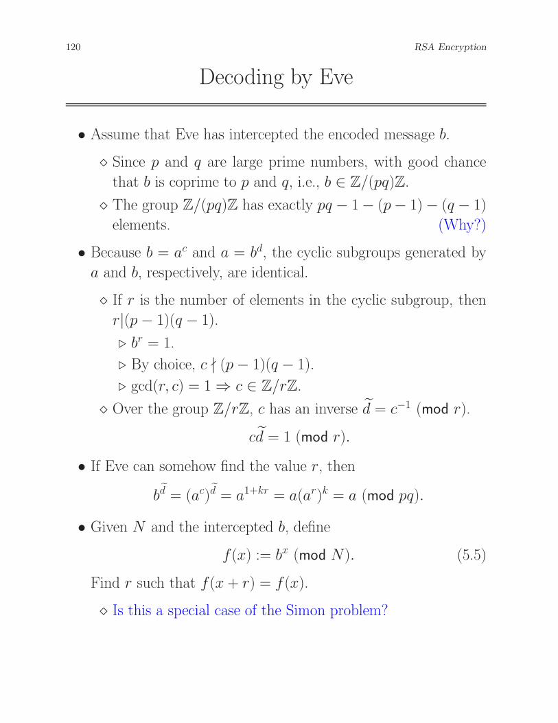
• Assume that Eve has intercepted the encoded message b.

⋄ Since p and q are large prime numbers, with good chance

that b is coprime to p and q, i.e., b ∈ Z/(pq)Z.

⋄ The group Z/(pq)Z has exactly pq − 1− (p− 1)− (q − 1)

elements. (Why?)

• Because b = ac and a = bd, the cyclic subgroups generated by

a and b, respectively, are identical.

⋄ If r is the number of elements in the cyclic subgroup, then

r|(p− 1)(q − 1).

⊲ br = 1.

⊲ By choice, c ∤ (p− 1)(q − 1).

⊲ gcd(r, c) = 1 ⇒ c ∈ Z/rZ.

⋄ Over the group Z/rZ, c has an inverse d = c−1 (mod r).

cd = 1 (mod r).

• If Eve can somehow find the value r, then

bd = (ac)d = a1+kr = a(ar)k = a (mod pq).

• Given N and the intercepted b, define

f(x) := bx (mod N). (5.5)

Find r such that f(x + r) = f(x).

⋄ Is this a special case of the Simon problem?

5.2. QUANTUM FOURIER TRANSFORM 121

5.2 Quantum Fourier Transform

• The discrete Fourier transform (DFT) is the equivalent of the

continuous Fourier transform for signals known only at finitely

many instants separated by sample times.

• The quantum Fourier transform (QFT) assumes a similar form

but has an entirely different meaning.

• The fast Fourier transform (FFT) exploits the structure of DFT

and is critical in modern applications.

• The QFT is fast in its parallelism.

122 Quantum Fourier Transform

Quick Recap of Classical DFT

• Given samples {f0, f1, . . . , fN−1} of a signal at fixed intervals

in the time domain, the DFT in the frequency domain is defined

by

Fj :=1√N

N−1∑

k=0

e−ı2πN jkfk, j = 0, 1, . . . , N − 1. (5.6)

⋄ The relationship (5.6) can be expressed as

F = W f . (5.7)

⊲ The coefficient matrix W is unitary. (Prove this.)

⋄ Exploiting the cyclic nature in W leads to the fast Fourier

transform (FFT) which is one of the most important algo-

rithms with many applications.

⊲ At the cost of O(N log2N) computations.

⊲ Usually prefer that N = 2n. Therefore, the overhead of

FFT is O(n2n).

X The significance of QFT is that the overhead is O(n2),

i.e., exponentially faster than fast.

• It is easy to check the inverse relationship (IDFT):

fj :=1√N

N−1∑

k=0

eı2πN jkFk, j = 0, 1, . . . , N − 1. (5.8)

• Some scholars/books weight the coefficient matrices differently

for the convenience of trigonometric interpolation.

Applications 123

n-qubit QFT

• LetN := 2n. The n-qubit quantum Fourier transform (QFT)

is a unitary transformation UFT defined by

UQFT |k〉n :=1√N

N−1∑

j=0

e−ı2πN jk |j〉n . (5.9)

• Suppose that g : ZN → C. Consider its vector representation

g =N−1∑

k=0

g(k) |k〉n .

Then

UQFT (g) =N−1∑

k=0

g(k)1√N

N−1∑

j=0

e−ı2πN jk |j〉n

=

N−1∑

j=0

(1√N

N−1∑

k=0

g(k)e−ı2πN jk) |j〉n

=N−1∑

j=0

G(j) |j〉n .

⋄ The Fourier coefficients of g are defined as

G(j) :=1√N

N−1∑

k=0

g(k)e−ı2πN jk. (5.10)

⊲ In complete sync with (5.6).


Confusing Notation

• Conventions for the sign of the phase factor exponent vary.

Some literature prefers to define the n-qubit QFT via

U†FT |j〉n :=

1√N

N−1∑

k=0

eı2πN jk |k〉n . (5.11)

⋄ This is indeed a resemblance to the IDFT in (5.8).

• Though look alike, do not confused U†FT with (3.12) where

H⊗n |j〉n =1√N

N−1∑

k=0

eıπj·k |k〉n .

⋄ The product jk in (5.9) is the ordinary multiplication, but

the product j · k is the bitwise inner product modulo 2.

⋄ eıπj·k = (−1)j·k are ±1, but eı2πN jk has many phases.

• An important question is to show that an n-qubit QFT can be

implemented out of 1-qubit and 2-qubit unitary gates and that

the number of gates grows only quadratically in n.

⋄ This realization, at least in theory, will become clear at the

end of of the next chapter on phase estimation.

Applications 125

Using QFT for Period Finding

• Consider as a demo the case n = 3 where we are looking for the

period of f : {0, 1}3 → {0, 1}3. (Simon Problem)

• Start with the initial state

|Ψ0〉 := H⊗3 |0〉3 =1√8

7∑

j=0

|j〉3 .

• Apply Uf to obtain

|Ψ1〉 := Uf(H⊗3 |0〉3 |0〉3) =

1√8

7∑

j=0

|j〉3 |f(j)〉3 .

⋄ All output registers are equally weighted.

• Apply the QFT to obtain

|Ψ2〉 := UQFT (|Ψ1〉) =1

8

7∑

j=0

7∑

k=0

e−ı2π8 jk |k〉3 |f(j)〉3

=1

8

7∑

k=0

|k〉3 (7∑

j=0

e−ı2π8 jk |f(j)〉3).

• Suppose that the period is p = 2. Define the abbreviation{a := f(0) = f(2) = f(4) = f(6),

b := f(1) = f(3) = f(5) = f(7).

⋄ Check the second summation sk :=∑7

j=0 e−ı2π8 jk |f(j)〉3.


• Define ωk := e−ı2π8 k. Then

sk = |a〉3 (ω0k + ω2

k + ω4k + ω6

k) + |b〉3 (ω1k + ω3

k + ω5k + ω7

k).

⋄ s0 = 4 |a〉3 + 4 |b〉3.⋄ s4 = 4 |a〉3 − 4 |b〉3.⋄ All other sk = 0.

• In short, after the quantum Fourier transform, we see a redis-

tribution of the weights, i.e.,

|Ψ2〉 =1

2(|0〉3 |a〉3 + |0〉3 |b〉3 + |4〉3 |a〉3 − |4〉3 |b〉3).

If we take the measurement, input registers |0〉 and |4〉 will showup with equal probability which is a consequence of p = 2.

• The cancelation observed here is more extensively exploited in

Shor’s factorization algorithm.

Applications 127

General Algorithm for N = 2n

• Prepare the uniform superposition of all basic |x〉.

|Ψ0〉 :=1√N

∑

x∈ZN

|x〉 .

• Apply the oracle Uf to obtain

|Ψ1〉 :=1√N

∑

x∈ZN

|x〉 |f(x)〉 .

• Measure an output register and take record of the input register

of the collapsed state.

• Apply QFT to the input register.

• Repeat enough times to create equations for estimating the pe-

riod p.


Analysis I

• Denote the image set of f by O.

⋄ O contains exactly p elements.

⋄ For each c ∈ O, define the indicator function fc : ZN →{0, 1} by

fc(x) =

{1 if f(x) = c,

0 otherwise.

• Rewrite |Ψ1〉 as

|Ψ1〉 =∑

c∈O

1√N

∑

x∈ZN

(fc(x) |x〉) |f(x)〉 .

⋄ The probability of observing c is 1p for every c ∈ O. (Why?)

⋄ At the observation c, the system collapse to

|Φ〉 :=

√p

N

∑

x∈ZN

(fc(x) |x〉) |c〉

=1√N

∑

x∈ZN

(√pfc(x) |x〉) |c〉 .

• Which output register c is to be measured?

Applications 129

Periodic Spike Function

• Given g : ZN → C, suppose g(k) = g(k + T ). Then

UQFT (g) =N−1∑

k=0

g(k)1√N

N−1∑

j=0

e−ı2πN jk |j〉n

=N−1∑

j=0

(1√N

N−1∑

k=0

g(k + T )e−ı2πN jk) |j〉

=

N−1∑

j=0

(1√N

N−1∑

y=0

g(y)e−ı2πN j(y−T )) |j〉

=

N−1∑

j=0

eı2πN jTG(j) |j〉 .

⋄ The Fourier coefficients of g and g have the same magnitude.

• Suffice to concentrate on one output register c.

• Without loss of generality, we take c = f(0).

⋄ fc(x) = 1 only at the set H = {0, p, 2p, 3p, . . .}.⋄ H has exactly N

p elements.


Analysis II

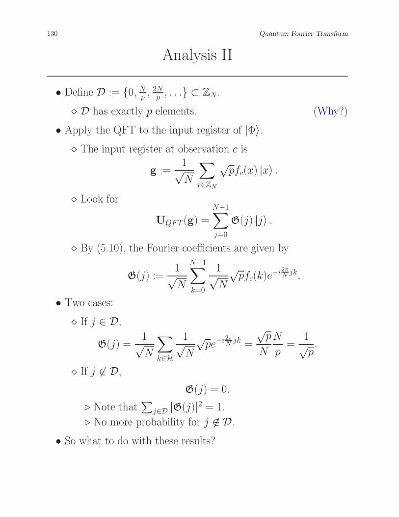
• Define D := {0, Np, 2Np, . . .} ⊂ ZN .

⋄ D has exactly p elements. (Why?)

• Apply the QFT to the input register of |Φ〉.⋄ The input register at observation c is

g :=1√N

∑

x∈ZN

√pfc(x) |x〉 .

⋄ Look for

UQFT (g) =

N−1∑

j=0

G(j) |j〉 .

⋄ By (5.10), the Fourier coefficients are given by

G(j) :=1√N

N−1∑

k=0

1√N

√pfc(k)e

−ı2πN jk.

• Two cases:

⋄ If j ∈ D,

G(j) =1√N

∑

k∈H

1√N

√pe−ı

2πN jk =

√p

N

N

p=

1√p.

⋄ If j 6∈ D,

G(j) = 0.

⊲ Note that∑

j∈D |G(j)|2 = 1.

⊲ No more probability for j 6∈ D.

• So what to do with these results?

Applications 131

Analysis III

• We measure each j ∈ D with probability 1pand others with

probability 0.

• j ∈ D if and only if jp = 0 (mod N).

⋄ That is, we sample a uniformly random j, which are multi-

ples of the ratio Np, such that jp = 0 (mod N).

• This is similar to what has happened in Simon algorithm!

⋄ In the Simon algorithm, we sampled a uniformly random

such that zi ⊥ p under the dot product of two n-qubit

modulo 2.

⋄ Here, we consider multiplication modulo N .

• How to find the ratio m = Np ?

⋄ The algorithm samples a random integer multiple of m.

⋄ Suppose we have two random samples, which we can write

am and bm.

⋄ Note that gcd(am; bm) = gcd(a; b)m, if gcd(a; b) = 1, then

m is found.

• If a and b are uniformly and independently sampled integers

from ZN , what is the probability that gcd(a; b) = 1?

132 Shor Factorization

5.3 Shor Factorization

• Shors factorization algorithm is used to factor numbers into their

components (which can potentially be prime).

• It is one of the most significant examples in which a quantum

computer demonstrates enormous power surpassing its classical

counterpart.

⋄ The algorithm does the factorization in roughly O(n3) quan-

tum operations.

⋄ In contrast, the best known classical algorithms are expo-

nential.

• Since the basis of most modern cryptography system is relying

on the impossibility of exponential cost of factorization, being

able to factor in polynomial time on a quantum computer has

attracted significant interest.

Applications 133

Basic Idea

• Given positive integers x and N , x < N , x is coprime to N ,

the order of x (mod N) is the least positive integer r such that

xr (mod N) = 1.

⋄ Since x (mod N) can only take a finite number of different

values, x must have a finite order, denoted by ordN(x).

⋄ The order ordN(x) divides the order of Z/NZ.

• A basic idea of Shor’s algorithm:

⋄ Suppose p and q are prime number and N = pq.

⋄ Choose some random x which is co-prime of N

⋄ Use quantum parallelism to compute xr for all r simultane-

ously. (This is only an easy brute force way. It could be

done in a better way.)

⋄ Interfere all of the xr’s to obtain knowledge about its period.

⋄ Use this period to find the factor p or q of N .


Order Finding ⇒ Factorization

• A quantum computation is needed to find the order r, which

will be discussed later.

• If the order r of x is odd, choose another random x.

• Suppose an even order r is found. Write

(xr/2 − 1)(xr/2 + 1) = xr − 1 = 0 (mod N).

⋄ If xr/2+ 1 = 0 (mod N), then gcd(xr/2− 1, N) = 1; choose

a different x.

⋄ If xr/2 + 1 6= 0 (mod N), then

d := gcd(xr/2 − 1, N)

must be either p or q.

⊲ xr/2 − 1 cannot be a multiple of N ; otherwise, xr/2 =

1 (mod N), contradicting ordN(x) = r.

⊲ xr/2 − 1 contains either p or q.

• No need to assume N = pq.

⋄ The number d gives us a nontrivial factor of N .

⋄ Factorize d and Ndrecursively and obtain all prime factors.

⋄ We can efficiently test primality. (How?)

• SupposeN has at least two distinct prime factors. If x ∈ Z/NZ

is selected randomly, then the probability that ordN(x) is even

and is at least 12.

Applications 135

Order Finding

• Choose n large enough such that N2 < Q := 2n < 2N2. Define

f : ZQ → ZN via

f(z) := xz (mod N).

⋄ Finding ordN(x) is almost equivalent to finding the period

of f .

f(z + r) = f(z).

⋄ However, r does not necessarily divide Q. This is the main

difference between order-finding and period finding.

• For a measurement of the output register c,

⋄ It appears only D times where D is either ⌊Qr⌋ or ⌈Q

r⌉.

⋄ The system collapse to

|Φ〉 :=1√D

∑

z∈ZQ

(fc(z) |z〉) |c〉 .

⋄ Replace the setD used in Analysis II byD := {0, D, 2D, . . .}.⋄ Apply the QFT to |Φ〉 to obtain

(UQFT ⊗ I)(|Φ〉) =Q−1∑

j=0

G(j) |j〉 |c〉 .

with the Fourier coefficients

G(j) :=1√QD

Q−1∑

k=0

fc(k)e−ı2πQ jk =

1√QD

D−1∑

t=0

e−ı2πQ jtr

⊲ This is not as simple as that for the period-finding.


Continued Fraction

(This is to be completed later.)

5.4. SOLVING LINEAR ALGEBRA PROBLEMS 137

5.4 Solving Linear Algebra Problems

• Eigenvalue Problem

• Quantum Phase Estimation

• System of Linear Equations

138 Linear Systems

Eigenvalue Problem

• Given a unitary operator U that operates on m qubits with an

eigenvector |Ψ〉 such that

U |Ψ〉 = eı2πω |Ψ〉 ,

estimate ω.

⋄ With high probability;

⋄ Within additive error ǫ;

⋄ Using O(log 1ǫ) qubits;

⋄ Using O(1ǫ) controlled-U operations.

• The following process Uphase that does the transformation

|0〉n |Ψ〉 → |ω〉 |Ψ〉

is called a quantum phase algorithm.

⋄ ω is an estimate of ω with known error.

Applications 139

Setup

• Create superposition:

|Φ〉 = (H⊗n ⊗ I)(|0〉⊗n |Ψ〉) = 1√2n(|0〉 + |1〉)⊗n |Ψ〉 .

• Apply controlled-U2j gates, j = 0, 1, . . . , n − 1, sequentially

according to the circuit:

|0〉 H •

|Φ〉

... ...

|0〉 H •

|0〉 H •

|0〉 H •

|Ψ〉 U20U21

U22 · · · U2n−1 |Ψ〉

140 Linear Systems

⋄ First, apply the controlled-U20:

|Ψ〉 cU20

⇒ 1√2n(|0〉 + |1〉)⊗(n−1) ⊗ (|0〉 |Ψ〉 + |1〉U20 |Ψ〉

= (1√2n(|0〉 + |1〉)⊗(n−1) ⊗ (|0〉 + eı2π2

0ω |1〉))⊗ |Ψ〉 .

⋄ Followed by the controlled-U21:

cU21

⇒ 1√2n(|0〉+|1〉)⊗(n−3)⊗(|0〉+eı2π21ω |1〉)⊗(|0〉+eı2π20ω |1〉)⊗|Ψ〉 .

⋄ At the end, receive the identity for the input register:

n⊗

j=1

1√2(|0〉 + eı2πω2

n−j |1〉) = 1√2n

2n−1∑

k=0

eı2πωk |k〉n . (5.12)

⊲ Prove the identity!

⊲ Same problem, but without the knowledge of |Ψ〉.⊲ Estimate ω.

Applications 141

Quantum Phase Estimation

• Problem: Given a state

|Φ〉 := 1√2n

2n−1∑

k=0

eı2πωk |k〉n , (5.13)

obtain a good estimate of the phase parameter ω.

• Some preliminary facts:

⋄ Because 0 < ω < 1, can express

ω = (.d1d2d3 . . .)2 =d12+d222

+ . . .

⋄ Then

eı2π(2kω) = eı2π(d1d2d3...dk.dk+1dk+2...)2

= eı2π(0.dk+1dk+2...)2

⋄ Therefore, can rewrite |Φ〉 as

|Φ〉 =n⊗

j=1

1√2(|0〉 + eı2π(.dn−j+1dn−j+2...)2 |1〉).

142 Linear Systems

An Example

• Consider the case n = 2 and ω = (.d1d2)2.

• By (5.12),

|Φ〉 = (|0〉 + eı2π(.d2)2 |1〉√

2)⊗ (

|0〉 + eı2π(.d1d2)2 |1〉√2

).

• Applying H to the first qubit, we see that

H(|0〉 + eı2π(.d2)2 |1〉√

2) =

|0〉 + |1〉2

+|0〉 − |1〉

2(−1)d2 = |d2〉 .

• To determine d1,

⋄ If d2 = 0, obtain d1 by applying H to the second qubit.

⋄ If d2 = 1,

⊲ Define the 1-qubit phase rotation operator R2

R2 :=

[1 0

0 eı2π22

]. (5.14)

.

⊲ Observe

R−12 (

|0〉 + eı2π(.d11)2 |1〉√2

) =|0〉 + eı2π(.d1)2 |1〉√

2.

⋄ This is a controlled-R−12 gate.

• The phase can be recovered exactly from the circuit:

|0〉+eı2π(.d2)2 |1〉√2

H • |d2〉|0〉+eı2π(.d1d2)2 |1〉√

2ON MLHI JKR−1

2 H |d1〉

Applications 143

Generalization

• Consider the case n = 3 and ω = (.d1d2d3)2.

• By (5.12),

|Ψ〉 = (|0〉 + eı2π(.d3)2 |1〉√

2)⊗(

|0〉 + eı2π(.d2d3)2 |1〉√2

)⊗(|0〉 + eı2π(.d1d2d3)2 |1〉√

2).

• Define the phase rotation operator Rk by

Rk :=

[1 0

0 eı2π2k

]. (5.15)

.

• Build the circuit as

|0〉+eı2π(.d3)2 |1〉√2

H • • |d3〉|0〉+eı2π(.d2d3)2 |1〉√

2ON MLHI JKR−1

2 H • |d2〉

|0〉+eı2π(.d1d2d3)2 |1〉√2

ON MLHI JKR−13

ON MLHI JKR−12 H |d1〉

• Note that the above operations does the inverse of QFT.

1√23

23−1∑

k=0

eı2π(.d1d2d3)2k |k〉n → |d1d2d3〉 .

144 Linear Systems

Inverse QFT

• Recall the linear relationships F = W f in the DFT and f =

W ∗F in the IDFT.

⋄ Is there a similar inverse relationship to the QFT (5.9)?

• In the above construction, ω is of the form x2n

where x is an

n-qubit, i.e.,

1√2n

2n−1∑

k=0

eı2π2nxk |k〉n → |x〉 . (5.16)

⋄ By applying the circuit in reverse order whereas every gate

is replaced by its inverse, we have a circuit for the QFT.

⋄ Show that the transformation (5.16) can be expressed as the

map

UQFT |j〉n :=1√2n

2n−1∑

k=0

e−ı2π2n jk |k〉n . (5.17)

• What if ω is not of the form x2n, say, what if ω is irrational?

Applications 145

Quantum Phase Algorithm

• Applying the QFT to the right side of (5.12) yields

UQTF |Φ〉 =1√2n

2n−1∑

k=0

eı2πωkUQFT |k〉n

=1√2n

2n−1∑

k=0

eı2πωk1√2n

2n−1∑

j=0

e−ı2π2n jk |j〉n

=1

2n

2n−1∑

j=0

(

2n−1∑

k=0

eı2πk

2n (2nω−j)) |j〉n

• Approximate the value of ω ∈ [0, 1] as follows:

⋄ Round 2nω to the nearest integer, say,

2nω = a + 2nδ,

with 0 ≤ δ ≤ 12n+1 .

⋄ The final state appears in the form

1

2n

2n−1∑

x=0

2n−1∑

k=0

e−ı2πk

2n (x−a)eı2πδk |x〉 ⊗ |Ψ〉 .

⋄ Make a measurement. The probability of yielding x = a is

given by

Pr(x = a) =1

22n

∣∣∣∣∣2n−1∑

k=0

eı2πδk

∣∣∣∣∣

2

=

1, if δ = 0,

122n

∣∣∣1−eı2π2nδ

1−eı2πδ

∣∣∣2

, if δ 6= 0.

⊲ Can prove that for δ 6= 0, Pr(a) ≥ 4π2 ≈ 0.40.

146 Linear Systems

System of Linear Equations

• Solving linear systems is fundamental in virtually all areas of sci-

ence and engineering. A quantum algorithm for linear systems

of equations has the potential for widespread applicability.

• Thus far, the quantum algorithm can only work for Hermitian

matrices, preferably large and sparse.

• Can provide only a scalar measurement on the solution vector.

Not the values of the solution vector itself.

⋄ What to expect from a quantum machine when trying to

determine the intersection of two lines? Can quantum com-

puting determine the geometry?

Applications 147

Quantum Linear System Problem

• Given an N ×N Hermitian matrix A, a unit vector b, and an

operator M , find the value

〈x|M |x〉

where x is a solution to the system

A |x〉 = |b〉 .

• It has been declared that the quantum algorithm has an expo-

nential speedup, O(log2N), as opposed toO(N3) of the classical

Gaussian elimination method. However, we must clarify some

assumptions:

⋄ To merely read in the entries of the vector |b〉 will cost

O(N). So |b〉 is assumed to be already prepared by some

other means.

⋄ As a state, |b〉 must be normalized.

⋄ If we have a means to measure one component of |x〉, thesystem collapses. If we want to measure all components, we

must repeat the algorithm N times. This is exponentially

more than O(log2N).

⋄ The algorithm is suitable only for the class of quantum linear

system problems (QLSP).

148 Linear Systems

Basic Steps

• If A is Hermitian, then U := eıAt is unitary.

⋄ The eigenvalues λj of A must be real.

⋄ The eigenvalues of A are precisely the phases of U .

⋄ A and U have the same set of eigenvectors |Ψj〉.• Apply the phase estimation gate Uphase to Ψj, we have an esti-

mate λj of λj.

|0〉n |Ψj〉 →∣∣∣λj

⟩|Ψj〉

without knowing |Ψj〉.• Expand |b〉 in terms of the basis of eigenvectors,

|b〉 =N∑

j=1

βj |Ψj〉 .

⋄ Via Uphase, we obtain the transformation

|b〉 →N∑

j=1

βj

∣∣∣λj⟩|Ψj〉 .

• Add a third register (ancilla) to make a controlled rotation eıθY

conditioned upon∣∣∣λj

⟩to obtain

∣∣∣λj⟩|Ψj〉 →

∣∣∣λj⟩|Ψj〉 (

√1− (

γj

λj)2 |0〉 + γj

λj|1〉).

⋄ The control is per j and, hence, this is parallelism.

⋄ γj is for normalization.

Applications 149

• Together, the state is now

N∑

j=1

βj

∣∣∣λj⟩|Ψj〉 (

√1− (

γj

λj)2 |0〉 + γj

λj|1〉).

• Undo (reverse) the phase estimation to obtain

|0〉⊗n ⊗N∑

j=1

βj |Ψj〉 (√1− (

γj

λj)2 |0〉 + γj

λj|1〉).

• Employ an amplifying operator to enlarge the magnitude of |1〉.The second term is proportional to

A−1 |b〉 =N∑

j=1

βj1

λj|Ψj〉 .

⋄ The whole process is nothing but an analogue of the linear

algebra.

⊲ If A = QΛQ∗, then

A−1 = QΛ−1Q∗.

⊲ Therefore,

x = QΛ−1 Q∗b︸︷︷︸β1,...,βn

.

• Note that only a quantum description of the solution vector is

output from HHL.

⋄ For applications that need a full classical description of x,

this may not be satisfactory.

150 Differential Equations

5.5 Differential Equations

• Classical ODE Methods

• Quantum Formulations

Applications 151

Classical ODE Methods

• Differential equations are ubiquitous in science and engineer-

ing. Solving differential equations with high precision is of

paramount importance.

• Both the theory and techniques of numerical ODEmethods have

reached the state-of-the-art in digital computation.

⋄ Can be programmed to automatically adapt optimal step

sizes and orders along the integration.

⋄ Efficient for fast integration and effective for meeting error

tolerance.

• Two main basic notions:

⋄ Nonlinear one-step methods.

⊲ Self-sufficient.

⊲ Can be used for help generate starting values.

⊲ More expensive.

⋄ Linear multi-step methods.

⊲ Require starting values.

⊲ Much cheaper with higher order precision.


Euler Method

• The simplest numerical method,

⋄ If y(x) is a solution, then

y(xn + h) = y(xn) + hy′(xn) +O(h2)

is the Taylor series expansion of y(xn + h) near xn.

⋄ Suppose the accepted solution at xn is given y(xn) ≈ yn,

then the truncated Taylor series suggests a scheme:

yn+1 = yn + hf(xn, yn) (5.18)

should be a reasonable approximation.

• Questions always asked in numerical ODE:

⋄ What is the magnitude of the global error

en := yn − y(xn)

at the n-th step?

⋄ (Stability) How does the error propagate?

⋄ (Precision) How does the step size h affect the accuracy?

⋄ How to control the step size and error growth to get the best

possible accuracy?

Applications 153

An Improved Idea

• Consider a 2-stage scheme:

⋄ Take one half-step Euler shooting:

yn+12:= yn +

h

2f(xn, yn).

⋄ Use the midpoint, instead of the endpoint, to estimate the

slop:

fn+12:= f

(xn+1

2, yn+1

2

).

⋄ Take one full Euler shooting:

yn+1 = yn + hf

(xn +

h

2,yn +

h

2f(xn,yn)

).

• Note that there are two function evaluations involved.

⋄ This is a smart way to implement the Taylor’s series expan-

sion.

⋄ Can match up the terms up to O(h3).

⋄ The method has one-order better precision than the Euler

method.


Runge-Kutta Methods

• A general R-stage Runge-Kutta method is defined by the one-

step method:

yn+1 = yn + hφ(xn, yn, h) (5.19)

where

φ(xn, yn, h) =

R∑

r=1

crkr (5.20)

R∑

r=1

cr = 1

kr = f(xn + arh, yn + hR∑

s=1

brsks) (5.21)

R∑

s=1

brs = ar.

• It is convenient to characterize the scheme in the Butcher array:

a1 b11 b12 . . . b1Ra2 b21 b22 . . . b2R... ... ...

aR bR1 bR2 . . . bRRc1 c2 . . . cR

• Lots of research has been done in the past few decades to find

out the best combinations of these coefficients.

Applications 155

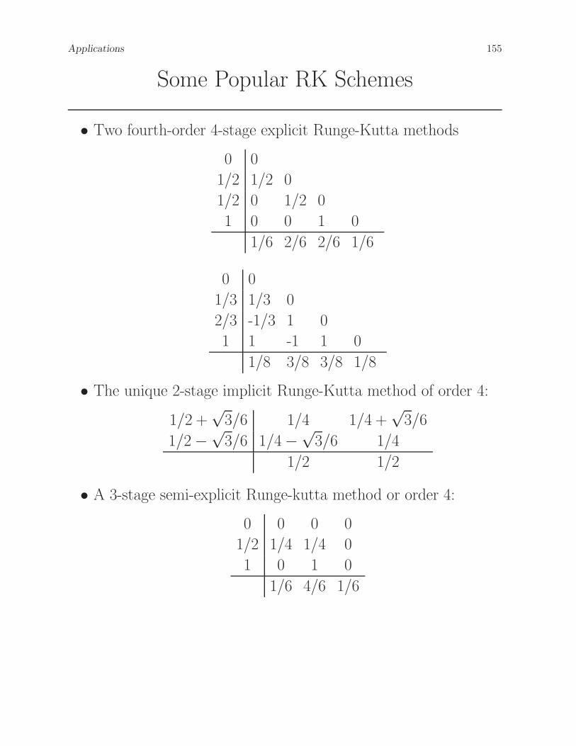
Some Popular RK Schemes

• Two fourth-order 4-stage explicit Runge-Kutta methods

0 0

1/2 1/2 0

1/2 0 1/2 0

1 0 0 1 0

1/6 2/6 2/6 1/6

0 0

1/3 1/3 0

2/3 -1/3 1 0

1 1 -1 1 0

1/8 3/8 3/8 1/8

• The unique 2-stage implicit Runge-Kutta method of order 4:

1/2 +√3/6 1/4 1/4 +

√3/6

1/2−√3/6 1/4−

√3/6 1/4

1/2 1/2

• A 3-stage semi-explicit Runge-kutta method or order 4:

0 0 0 0

1/2 1/4 1/4 0

1 0 1 0

1/6 4/6 1/6


Linear Multi-step Methods

• A linear (p+1)-step method of step size h is a numerical scheme

of the form

yn+1 =

p∑

i=0

aiyn−i + h

p∑

i=−1

bifn−i (5.22)

where xk = x0 + kh, fn−i := f(xn−i, yn−i), and a2p + b2p 6= 0.

⋄ Note that the information used involves past values the ap-

proximate solution yi and its first order derivative fi.

⋄ If b−1 = 0, then the method is said to be explicit; otherwise,

it is implicit.

⊲ In order to obtain yn+1 from an implicit method, usually

it is necessary to solve a nonlinear equation.

⊲ Implicit methods are more expensive.

⊲ Implicit methods has better stability.

• The Adams family:

yn+1 = yn +

p∑

i=−1

βpifn−i (5.23)

⋄ Obtained from the Fundamental Theorem of Calculus

y(xn+1)− y(xn) =

∫ xn+1

xn

f(x, y(x))dx.

⋄ The unknown f(x, y(x)) is approximated by polynomial in-

terpolation.

Applications 157

Some Popular Multi-step Schemes

• Some Adams-Bashforth methods:

0 1 2 3 4

β0i 1

2β1i 3 -1

12β2i 23 -16 5

24β3i 55 -59 37 -9

720β4i 1901 -2774 2616 -1274 251

• Some Adams-Moulton methods:

-1 0 1 2 3

β0i 1

2β1i 1 1

12β2i 5 8 -1

24β3i 9 19 -5 1

720β4i 251 646 -264 106 -19


Quantum Formulation

• A quantum algorithm for general nonlinear differential equa-

tions might be too ambitious.

⋄ The complexity of the simulation scaled exponentially in the

number of time-steps.

⋄ The quantum nonlinear Schrodinger equation is nonlinear in

the field operators, but it is still linear in the quantum state.

⋄ Most operators act linearly on quantum superpositions.

• A more natural application for quantum computers is linear

differential equations:

dy

dt= A(t)y + b(t); y(t0) = y0 ∈ CN . (5.24)

• Do we really have to solve an ODE by quantum algorithms?

⋄ The complexity of solving the differential equation in the

classical algorithm must be at least linear in N .

⋄ One goal of the quantum algorithm is to solve the differential

equation in time O(poly(logN)). (Is this really

important?)

⋄ Another goal is to provide efficient scaling in the evolution

in time T .

⋄ Can the numerical analysis community accept quantum al-

gorithms? (In terms of precision and

stability)

Applications 159

Feynman Clock

• If a quantum system moves stepwise forward and then backward

in time in equal increments, it would necessarily return to its

original state.

• Traditional algorithms utilize parallelization in space.

⋄ A supercomputer comprising many processors spatially dis-

tributes and advances the problem in single temporal incre-

ments.

• On a quantum machine, think about the possibility of setting

up a calculation that is parallel in time.

⋄ Different points in time has to be simultaneously calculated

on many processors.


Key Idea

• Assume tj = t0 + jh, yk ≈ y(tj), and a total of Nt steps are

taken over [t0, T ] (so Nt =T−t0Nt

).

• Wish to obtain the final state in the form

|ψ〉 =Nt∑

j=0

|tj〉 |yj〉 . (5.25)

⋄ Temporarily ignore the normalization.

⋄ By measuring the time register, we get the approximation

yj.

⋄ The probability of obtaining the final time is small 1Nt+1

.

(How to boost the probability?)

• Try the Euler’s method:

yn+1 = yn + h(A(tn)yn + bn).

• Code the solution at y2 via

I 0 0 0 0

−(I + A(t0)h) I 0 0 0

0 −(I + A(t1)h) I 0 0

0 0 −I I 0

0 0 0 −I I

y0

y1

y2

y3

y4

=

y0

b(t0)h

b(t1)h

0

0

.

⋄ Note that y3 = y4 = y2 artificially. Therefore, the proba-

bility of getting y2 is boosted from 13to 3

5.

⋄ This linear system is to be solved via the HHL algorithm.

Applications 161

Criticisms

• Is this a good idea? (All because of the uncertainty in

quantum computing.)

• To achieve high precision, Nt has to be extremely large.

• To know the intermediate solutions, lots of measurements need

be made.

• How to deal with stability? The error will grow.

Download - Applications - NCSU

Top Related