An Effective Constitutive Model for Lime Treated Soils1
V. Robin1,2, A. A. Javadi1, O. Cuisinier2, F. Masrouri22
1Computational Geomechanics Group, Department of Engineering, University of Exeter, United-Kingdom3
2LEMTA – UMR 7563 CNRS, Laboratoire d’Energetique et de Mecanique Theorique et Appliquee, Universite de Lorraine,4
France5
Abstract6
The effect of lime on the yield stress, and more generally the presence of structure in the soil, is usually
not accounted for in the design of geotechnical structures. As a result the potential of lime treatment or
of a structured soil has not been fully exploited. This paper presents a new formulation to account for the
effect of structure on the mechanical behaviour for structured soils. A constitutive model is proposed in
the framework of the Modified Cam Clay model to describe the behaviour of lime treated soils. The new
formulation introduces a limited number of additional parameters, all of which have a physical meaning and
can be obtained from an isotropic compression test. Due to similarity in behaviour of lime treated soils
and naturally structured soils, the formulation can be applied to both types of soil. It is shown that the
proposed model can successfully reproduce the main features of both structured soils such as maximum rate
of dilation at softening and degradation at yield. The model can be applied for any structured material
regardless of the origin of cementation.
Keywords:7
lime treated soils, structured soils, degradation, constitutive modelling.8
1. Introduction9
The use of on-site materials has become a central issue for civil engineering companies, but it is some-10
times difficult to deal with all the resources available on site. For soils with low mechanical characteristics,11
lime treatment appears to be an efficient method to improve their mechanical properties and allow their use12
in geotechnical earth structures (e.g. Little, 1995). The effects of the addition of lime on the soil parameters13
such as cohesion and friction angle have been extensively studied (e.g. Brandl, 1981). Nevertheless, lime is14
still mostly used to dry soils with high water contents and increase the bearing capacity. However, it is also15
generally known that adding lime leads to a significant increase of the yield stress and modifies other me-16
chanical parameters in compacted soils. In lime-treated soils, the modification of the mechanical behaviour17
results from several physico-chemical processes associated with the increase in calcium concentration and18
pH (i.e. cation exchange, pozzolanic reactions, etc...).19
Preprint submitted to Computers and Geotechnics November 29, 2014
brought to you by COREView metadata, citation and similar papers at core.ac.uk
provided by Open Research Exeter
From an economical point of view, it is becoming increasingly important to account for the properties20
of treated materials in the design of the geotechnical structures. However, despite its proven efficacy, the21
use of treated materials suffers from several major drawbacks: there is no reliable method to account for22
the structure in the calculations. At yield, and for an increasing mechanical loading, treated materials23
experience what is called the ”loss of structure”, resulting in the degradation of the structure in different24
ways. To model the behaviour of these materials, a constitutive law describing the behaviour at yield is a25
requirement.26
Some studies (Maccarini, 1987; Aversa, 1991; Leroueil and Vaughan, 1990; Liu and Carter, 2003; Flora27
et al., 2006) have shown that naturally structured soils and artificially treated materials have common28
mechanical features; artificial treatment appears to create a “structure” in the soil. In this paper, “structure”29
refers to Burland’s definition (Burland, 1990), and is seen as the combination of the fabric and the bonding of30
the soil skeleton. Fabric accounts for the arrangement of particles, which depends on the state of compaction31
and their geometry.32
Several constitutive models have been proposed for structured materials. Most of these models use the33
destructured state as reference to describe the mechanical behaviour of structured soils. Liu and Carter34
(2002) proposed a constitutive model, based on the Modified Cam Clay model (MCC), by adding three35
additional parameters to the original MCC (Roscoe and Burland, 1968). Since then, several enhancements36
(e.g. Horpibulsuk et al., 2010; Suebsuk et al., 2011) have been proposed. However, various modes of de-37
structuration have been identified, and the original formulation fails to model some of them. A number38
of other formulations have been developed (Kavvadas and Amorosi, 2000; Vatsala et al., 2001; Nova et al.,39
2003; Baudet and Stallebrass, 2004; Rouainia and Muir wood, 2000; Nguyen et al., 2014) and some of which40
give good agreement with experimental results. However, it often comes at the cost of a larger number of41
parameters, or high computational resources (e.g. mapping rule). Parameters do not always have a physical42
meaning, and some of them can be difficult to determine. All these limitations make these models difficult43
to be used in engineering practice.44
The main objective of this paper is to propose a general and simple formulation capable of fulfilling some45
fundamentals criteria regarding the degradation of the structure. This model must be capable of modelling46
any kind of degradations, and require a limited number of parameters to account for the maximum number47
of features of structured materials. These parameters should be rapidly obtained from classic experimental48
tests, and they all must have a physical meaning. To this end, the paper will focus on two aspects:49
• How can the key features of structured or lime treated materials be described?50
• How can these features be efficiently accounted for in a constitutive model?51
This paper is divided into four parts. The first part gives a review of the main characteristics of naturally52
and artificially structured materials that must be reproduced by the model. The second part introduces the53
2
theoretical framework chosen for the model for lime treated soils (MLTS) and the new formulation developed54
to model the degradation of the structure. In the third part, the developed formulation is used to calculate55
the compliance matrix and obtain the stress-strain relationship. Finally, in the last part, we assess the56
suitability of the model in predicting experimental results obtained from triaxial tests on artificially (i.e.57
lime treated) and naturally structured materials.58
2. Features of structured soils59
The mechanical behaviour of naturally and artificially structured material has been extensively studied60
(Leroueil and Vaughan, 1990; Gens and Nova, 1993; Burland et al., 1996; Cotecchia and Chandler, 2000;61
Malandraki and Toll, 2001; Cuisinier et al., 2008, 2011; Consoli et al., 2011; Oliveira, 2013; Robin et al.,62
2014a) and some specific features have been identified. Several studies have pointed out that naturally and63
artificially structured soils have a similar mechanical behaviour. In this section, we identify the key features64
common to naturally and artificially structured soils that should be properly reproduced by a model.65
2.1. Naturally structured soils66
It has been shown that naturally structured soils have a higher yield stress compared to the destructured67
state (Burland et al., 1996), the latter being usually considered as the reference state. For the same stress68
state, a higher yield stress leads to a higher void ratio at yield compared to the destructured state, called69
the additional void ratio ∆e. Once plastic deformations take place, one can observe that the additional70
void ratio decreases. Depending on the material, the additional void ratio can quickly or slowly decrease71
until the material reaches a normal compression line (ncl), which can correspond to the ncl of the reference72
state (ncld), or a different one, parallel to the reference ncl but vertically translated along the v axis (nclr)73
(Baudet and Stallebrass, 2004; Callisto and Rampello, 2004; Suebsuk et al., 2011). More generally, 4 modes74
of degradation can be identified (Figure 1):75
Mode 1: Destructuration takes place immediately at yield. The additional void ratio progressively de-76
creases until it converges toward the destructured state (Yong and Nagaraj, 1977; Lagioia and Nova,77
1995).78
Mode 2: Destructuration takes place immediately at yield, but it does not converge toward its destructured79
state. A different ncl appears parallel to the destructured state, but a residual additional void ratio80
still remains (Burland et al., 1996; Rampello and Callisto, 1998).81
Mode 3: No significant destructuration is observed immediately after yield. The process of degradation is82
initiated later on for a higher effective mean stress and the additional void ratio completely disappears83
(Callisto and Rampello, 2004).84
3

Mode 4: No destructuration is observed immediately after yield. The process of degradation is initiated85
later on for a higher effective mean stress. However, a residual additional void ratio remains (Rotta86
et al., 2003).87
103Effective mean stress p′1.35
1.40
1.45
1.50
1.55
1.60Specificvolumev(-) ncld
url
∆ei
Mode 1
Mode 2
Mode 3
Mode 4
Figure 1: The four different modes of destructuration in structured soils – ncld: Normal compression line of the destructured
state, url: Unloading-reloading line.
Additionally, the volumetric behaviour of naturally structured soils was compared with the destructured88
state by Leroueil and Vaughan (1990) on heavily overconsolidated specimens from drained triaxial test89
results. They identified two different mechanisms taking place. While the maximum rate of dilation was90
measured before the peak of the deviatoric stress for the destructured soil, it was observed after the peak91
of the deviatoric stress for structured soils. This is due to the structure, which binds soil particles together.92
To allow the particles to move freely, the structure has to be degraded first to release particles (Leroueil and93
Vaughan, 1990).94
2.2. Lime treated soils95
Several studies have shown that addition of lime leads to an increase of the yield stress compared to the96
untreated state (Tremblay et al., 2001; Ahnberg, 2007). As for naturally structured soils, the additional void97
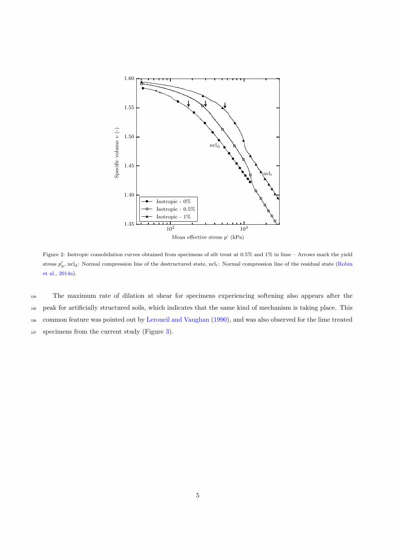
ratio appears to decrease at yield, i.e. the degradation of the artificial structure takes place. Robin et al.98
(2014a) have assessed the mechanical behaviour of a lime treated silt under isotropic loading (Figure 2). It99
can be seen that the mode of degradation depends on the amount of lime. For 0.5% in lime, the additional100
void ratio completely disappears at high stress states (Mode 3), when it is not the case for 1% lime treated101
specimens (Mode 4). This latter reaches a different ncl compared to the untreated specimen. Details about102
the samples and experimental conditions can be found in Robin et al. (2014a).103
4
102 103
Mean effective stress p’ (kPa)
1.35
1.40
1.45
1.50
1.55
1.60
Specificvolumev(-)
ncld
nclr
Isotropic - 0%
Isotropic - 0.5%
Isotropic - 1%
Figure 2: Isotropic consolidation curves obtained from specimens of silt treat at 0.5% and 1% in lime – Arrows mark the yield
stress p′y , ncld: Normal compression line of the destructured state, nclr: Normal compression line of the residual state (Robin
et al., 2014a).
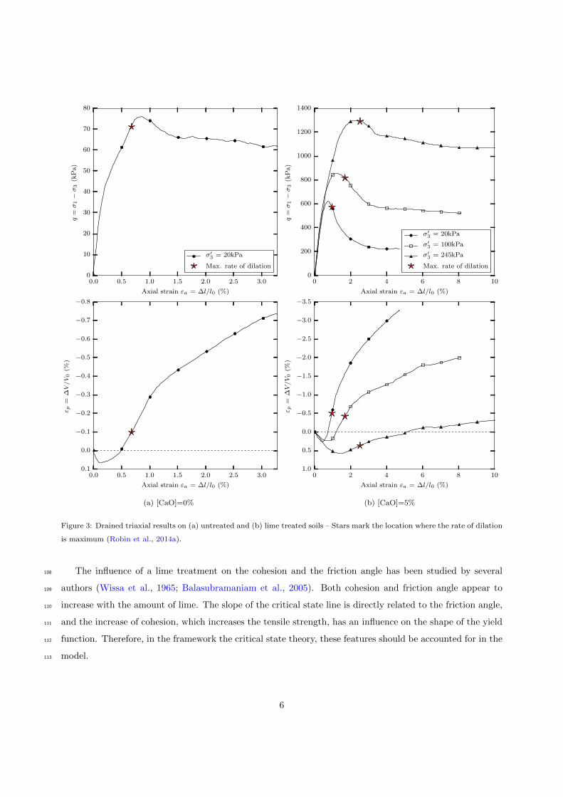
The maximum rate of dilation at shear for specimens experiencing softening also appears after the104
peak for artificially structured soils, which indicates that the same kind of mechanism is taking place. This105
common feature was pointed out by Leroueil and Vaughan (1990), and was also observed for the lime treated106
specimens from the current study (Figure 3).107
5
0.0 0.5 1.0 1.5 2.0 2.5 3.0
Axial strain εa = ∆l/l0 (%)
0
10
20
30
40
50
60
70
80
q=
σ1−
σ3(kPa)
σ′3 = 20kPa
Max. rate of dilation
0.0 0.5 1.0 1.5 2.0 2.5 3.0
Axial strain εa = ∆l/l0 (%)
−0.8
−0.7
−0.6
−0.5
−0.4
−0.3
−0.2
−0.1
0.0
0.1
ε p=
∆V/V0(%
)
(a) [CaO]=0%
0 2 4 6 8 10
Axial strain εa = ∆l/l0 (%)
0
200
400
600
800
1000
1200
1400
q=
σ1−
σ3(kPa)
σ′3 = 20kPa
σ′3 = 100kPa
σ′3 = 245kPa
Max. rate of dilation
0 2 4 6 8 10
Axial strain εa = ∆l/l0 (%)
−3.5
−3.0
−2.5
−2.0
−1.5
−1.0
−0.5
0.0
0.5
1.0
ε p=
∆V/V0(%
)
(b) [CaO]=5%
Figure 3: Drained triaxial results on (a) untreated and (b) lime treated soils – Stars mark the location where the rate of dilation
is maximum (Robin et al., 2014a).
The influence of a lime treatment on the cohesion and the friction angle has been studied by several108
authors (Wissa et al., 1965; Balasubramaniam et al., 2005). Both cohesion and friction angle appear to109
increase with the amount of lime. The slope of the critical state line is directly related to the friction angle,110
and the increase of cohesion, which increases the tensile strength, has an influence on the shape of the yield111
function. Therefore, in the framework the critical state theory, these features should be accounted for in the112
model.113
6
2.3. Summary114
Based on the previous observations, a model for lime treated soils might be suitable for naturally struc-115
tured soils, and therefore should be able to reproduce the four modes of destructuration and account for the116
following features:117
• The cohesion increases following pozzolanic reactions,118
• The yield stress increases for lime treated soils compared to the reference state,119
• At yield, there exists an additional void ratio compared to the reference state,120
• At yield, degradation of the structure takes place, which follows one of the four modes identified121
previously,122
• Overconsolidated specimens at shear show a maximum rate of dilation after the peak, describing the123
degradation of the structure,124
• The friction angle is modified due to the effects of the chemical reactions on the texture of the soil,125
and therefore the critical state as well.126
3. Theoretical framework of the model127
The model proposed in this paper was developed in the framework of the Modified Cam Clay model128
(MCC) to model the key features of lime treated soils previously identified. The new parameters introduced129
to model the degradation have all a physical meaning and can be determined from an isotropic compression130
test (Robin et al., 2014b). We present in this section a new formulation to model the four modes of131
degradation in structured soils under isotropic loading. This will then be used as a hardening rule for the132
determination of the compliance matrix.133
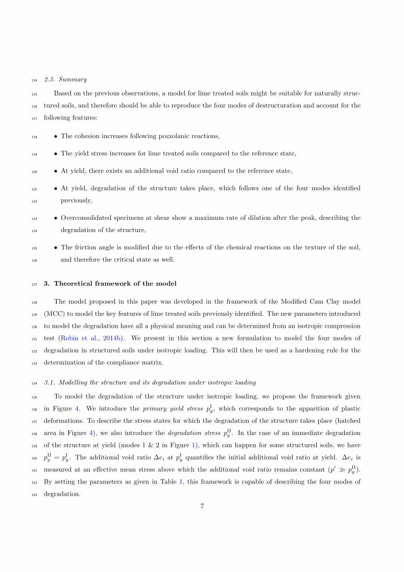
3.1. Modelling the structure and its degradation under isotropic loading134
To model the degradation of the structure under isotropic loading, we propose the framework given135
in Figure 4. We introduce the primary yield stress pIy, which corresponds to the apparition of plastic136
deformations. To describe the stress states for which the degradation of the structure takes place (hatched137
area in Figure 4), we also introduce the degradation stress pIIy . In the case of an immediate degradation138
of the structure at yield (modes 1 & 2 in Figure 1), which can happen for some structured soils, we have139
pIIy = pIy. The additional void ratio ∆ei at pIy quantifies the initial additional void ratio at yield. ∆ec is140
measured at an effective mean stress above which the additional void ratio remains constant (p′ � pIIy ).141
By setting the parameters as given in Table 1, this framework is capable of describing the four modes of142
degradation.143
7
In this study, the structure is quantified through the additional void ratio in comparison to the ncld and144
is assumed to be made of two components. The first one, referred to as the available structure, corresponds145
to the part of structure that will be available during the process of destructuration (∆ei − ∆ec). The146
second one, referred to as the residual structure, corresponds to the persisting additional void ratio at high147
effective mean stress (∆ec at p′ � pIy). The latter can be the consequences of chemical reactions, e.g. a lime148
treatment, which leads to a permanent modification of the fabric of the soil (Robin et al., 2014a).149
0 200 400 600 800 1000 1200 1400 1600p’
1.40
1.45
1.50
1.55
1.60
Specificvolumev(-)
ncld
nclr
url
∆ei
∆ec
Structured Soil
pIIypIy
Figure 4: General framework of the degradation of structured soils – ∆ei: Initial additional void ratio, ∆ec: Residual addi-
tional void ratio, pIy : Primary yield stress, pIIy : degradation stress, hatched area: degradation of the structure, ncld: Normal
compression line of the destructured state, nclr: Normal compression line of the residual state, url: Unloading-reloading line.
Table 1: Conditions on the parameters pIIy and ∆ec for the 4 modes of degradation
ParametersValues
Mode 1 Mode 2 Mode 3 Mode 4
pIIy pIy pIy > pIy > pIy
∆ec 0 > 0 0 > 0
3.1.1. Mathematical Formulation150
To model these four mechanisms, a flexible formulation using all the parameters previously introduced is
required. Richards’s equation (Richards, 1959) for the sigmoid provides many degrees of freedom to control
the shape of the function. This function is frequently used for the modelling natural phenomenons where
there exists a threshold above which a process is activated, in this case the degradation. This equation can
be written as follows:
∀p′ ∈[pIy,+∞
[π(p′) = 1− 1
1 + e−β(p′−pIIy )
(1)
8
where pIIy [Pa] corresponds to the position of the inflection point (π′′(pIIy ) = 0) and describes the stress151
state for which the degradation occurs (hatched area in Figure 4), and β [Pa−1] describes the rate of152
degradation.153
Therefore, we have
∀p′ ∈ R 0 ≤ π(p′) ≤ 1 (2)
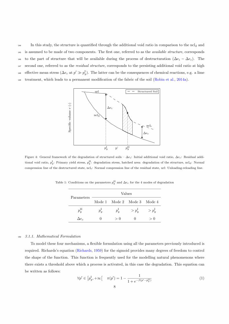
3.1.2. Scaling of π154
The function π is scaled to ensure that ∀β, ∀pIIy π(pIy) = 1, which leads to the following final formulation:
∀p′ ∈[pIy,+∞
[π(p′) =
eβpIy + eβp
IIy
eβp′ + eβpIIy
(3)
which verifies π(pIy) = 1 and limp′→+∞
π(p′) = 0.155
The ability to control the rate of degradation at yield of this formulation is demonstrated in Figure 5. It156
can be seen that the function π can either slowly decrease with a low β or quickly with a high β as p′ gets157
close to pIIy .158
100 150 200 250 300
p′(kPa)
0.00
0.05
0.10
0.15
0.20
β(kPa−1)
0.9
0.7
0.5
0.3
0.1
0.0 0.1 0.2 0.3 0.4 0.5 0.6 0.7 0.8 0.9 1.0
π(p′, β) = eβpIy+e
βpIIy
eβp′+eβpIIy
Figure 5: π values as a function of pIIy and β – pIy=100 kPa, pIIy =200 kPa.
9
3.1.3. Relationship between the specific volume and the effective mean stress for structured soils159
The presence of structure can be accounted for in the relationship between the specific volume and the
effective mean stress (v : p′ relationship) using the following general formulation:
∀p′ ∈ R∗+ v(p′) = Nλ − λ ln(p′) + ∆e(p′) (4)
with Nλ the intercept on the reference normal compression line ncld and λ the slope of the reference ncl160
in v : ln(p′) plane.161
Using the function π (Equation 3), the equation for the additional void ratio is given by:162
∀p′ ∈[pIy,+∞
[∆e (p′) = (∆ei −∆ec) ·
[eβp
Iy + eβp
IIy
eβp′ + eβpIIy
]+ ∆ec (5)
which fulfils the boundary value problems:
∆e(p′) =
∆ei if p′ = pIy
∆ec if p′ → +∞(6)
Introducing Equation 5 in Equation 4 gives the final equation of the specific volume for structured soils
at yield:
∀p′ ∈[pIy,+∞
[vs(p
′) = Nλ − λ ln(p′) + (∆ei −∆ec) ·[eβp
Iy + eβp
IIy
eβp′ + eβpIIy
]+ ∆ec (7)
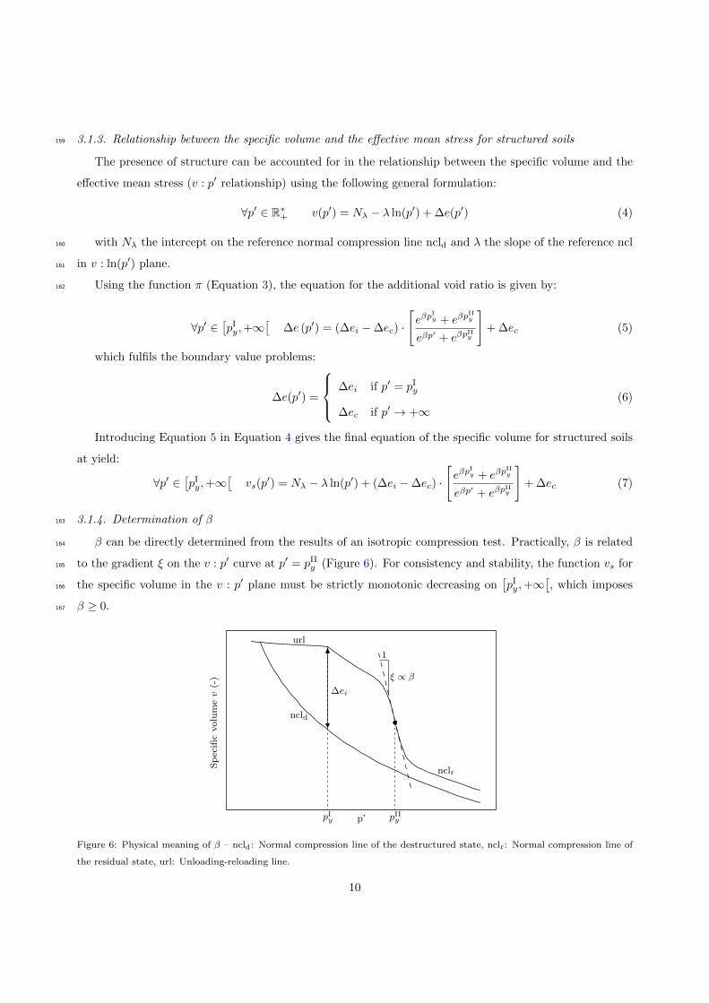
3.1.4. Determination of β163
β can be directly determined from the results of an isotropic compression test. Practically, β is related164
to the gradient ξ on the v : p′ curve at p′ = pIIy (Figure 6). For consistency and stability, the function vs for165
the specific volume in the v : p′ plane must be strictly monotonic decreasing on[pIy,+∞
[, which imposes166
β ≥ 0.167
0 200 400 600 800 1000 1200 1400 1600p’
1.40
1.45
1.50
1.55
1.60
Specificvolumev(-)
1
ξ ∝ β
∆ei
ncld
nclr
url
pIIypIy
Figure 6: Physical meaning of β – ncld: Normal compression line of the destructured state, nclr: Normal compression line of
the residual state, url: Unloading-reloading line.
10

Calling ξ the gradient of the specific volume curve at p′=pIIy , the appropriate value for β is obtained by
solving the following equation:(dv
dp′
)p′=pIIy
= ξ ⇔ −1
4
(1 + eβ(p
Iy−pIIy )
)× β(∆ei −∆ec)−
λ
pIIy= ξ (8)
There is no analytical solution to this equation, known as the Lambert W function, due to the non-168
linearity in β. However, this equation can be solved graphically or numerically using methods such as the169
Newton-Raphson algorithm (Corless et al., 1996).170
3.1.5. Suitability of the formulation171
The v : p′ relationship (Equation 7) is used to demonstrate the ability of the formulation to describe172
the four modes (Figure 7). Parameters used for the simulations are given in Table 2. The influence of173
the parameters β (Figure 8) and the degradation stress pIIy (Figure 9) is assessed and the case pIy = pIIy is174
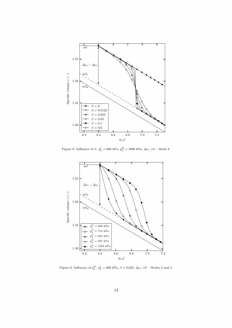
considered in Figure 10.175
Figure 8 shows that it is possible to describe the mode 3. Changing the value of β permits to achieve176
different rates of degradation. In this figure, a non-zero ∆ec was chosen (∆ec > 0), but mode 4 can be177
achieved by setting ∆ec = 0. The influence of pIIy is shown in Figure 9. One can see that this parameter178
controls the initiation of the process of degradation, and is successful in describing modes 2 and 4. As179
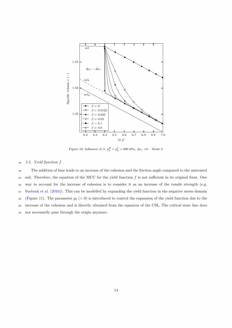
previously, modes 1 and 3 can be achieved by setting ∆ec = 0. Finally, the case pIy = pIIy is considered in180
Figure 10. This case corresponds to an immediate loss of structure at yield. This case does not lead to any181
instabilities of the formulation.182
11

6.2 6.4 6.6 6.8 7.0 7.2
ln p′
1.40
1.45
1.50
1.55
Specificvolumev(−
)
ncld
nclr
url
∆ei
Mode 1
Mode 2
Mode 3
Mode 4
Figure 7: Possibility of the formulation to model the four modes – ncld: Normal compression line of the untreated state, url:
Unloading-reloading line.
Table 2: Model parameters used for simulations of the four modes in Figure 7
Mode pIy (kPa) pIIy (kPa) ∆ei ∆ec β (kPa−1)
Mode 1 600 600 0.104 0.0 0.025
Mode 2 600 600 0.104 0.026 0.02
Mode 3 600 900 0.104 0.0 0.025
Mode 4 600 900 0.104 0.052 0.02
12
6.2 6.4 6.6 6.8 7.0 7.2
ln p′
1.40
1.45
1.50
1.55
Specificvolumev(−
)
ncld
nclr
url
∆ei −∆ec
β = 0
β = 0.0125
β = 0.025
β = 0.05
β = 0.1
β = 0.6
Figure 8: Influence of β: pIy = 600 kPa, pIIy = 1000 kPa, ∆ec >0 – Mode 4.
6.2 6.4 6.6 6.8 7.0 7.2
ln p′
1.40
1.45
1.50
1.55
Specificvolumev(−
)
ncld
nclr
url
∆ei −∆ec
pIIy = 600 kPa
pIIy = 712 kPa
pIIy = 825 kPa
pIIy = 937 kPa
pIIy = 1050 kPa
Figure 9: Influence of pIIy : pIy = 600 kPa, β = 0.025, ∆ec >0 – Modes 2 and 4.
13
6.2 6.3 6.4 6.5 6.6 6.7 6.8 6.9 7.0
ln p′
1.45
1.50
1.55
Specificvolumev(−
)
ncld
nclr
url
∆ei −∆ec
β = 0
β = 0.0125
β = 0.025
β = 0.05
β = 0.1
β = 0.6
Figure 10: Influence of β: pIIy = pIy = 600 kPa, ∆ec >0 – Mode 2.
3.2. Yield function f183
The addition of lime leads to an increase of the cohesion and the friction angle compared to the untreated184
soil. Therefore, the equation of the MCC for the yield function f is not sufficient in its original form. One185
way to account for the increase of cohesion is to consider it as an increase of the tensile strength (e.g.186
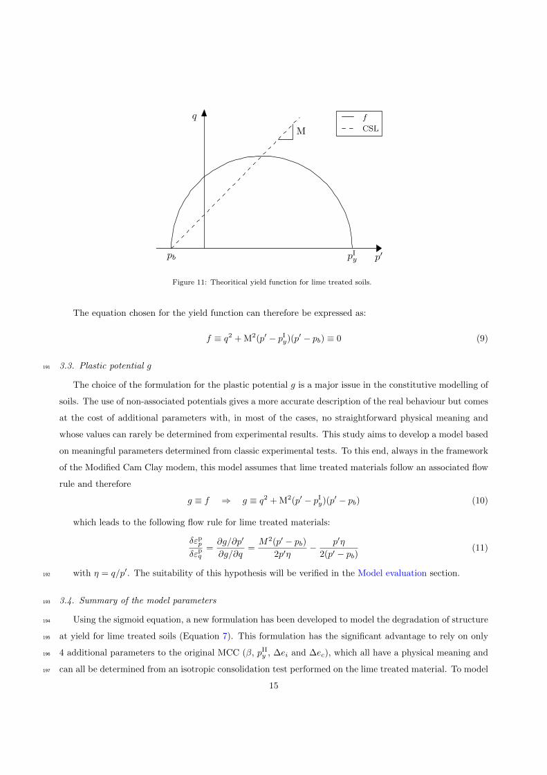
Suebsuk et al. (2010)). This can be modelled by expanding the yield function in the negative stress domain187
(Figure 11). The parameter pb (< 0) is introduced to control the expansion of the yield function due to the188
increase of the cohesion and is directly obtained from the equation of the CSL. The critical state line does189
not necessarily pass through the origin anymore.190
14
−20 0 20 40 60 80 100p′
q
pb pIy
M
f
CSL
Figure 11: Theoritical yield function for lime treated soils.
The equation chosen for the yield function can therefore be expressed as:
f ≡ q2 + M2(p′ − pIy)(p′ − pb) ≡ 0 (9)
3.3. Plastic potential g191
The choice of the formulation for the plastic potential g is a major issue in the constitutive modelling of
soils. The use of non-associated potentials gives a more accurate description of the real behaviour but comes
at the cost of additional parameters with, in most of the cases, no straightforward physical meaning and
whose values can rarely be determined from experimental results. This study aims to develop a model based
on meaningful parameters determined from classic experimental tests. To this end, always in the framework
of the Modified Cam Clay modem, this model assumes that lime treated materials follow an associated flow
rule and therefore
g ≡ f ⇒ g ≡ q2 + M2(p′ − pIy)(p′ − pb) (10)
which leads to the following flow rule for lime treated materials:
δεppδεpq
=∂g/∂p′
∂g/∂q=M2(p′ − pb)
2p′η− p′η
2(p′ − pb)(11)
with η = q/p′. The suitability of this hypothesis will be verified in the Model evaluation section.192
3.4. Summary of the model parameters193
Using the sigmoid equation, a new formulation has been developed to model the degradation of structure194
at yield for lime treated soils (Equation 7). This formulation has the significant advantage to rely on only195
4 additional parameters to the original MCC (β, pIIy , ∆ei and ∆ec), which all have a physical meaning and196
can all be determined from an isotropic consolidation test performed on the lime treated material. To model197
15

the influence of the cohesion on the deviatoric behaviour the parameter pb, directly related to the equation198
of the CSL, was introduced. As a conclusion, the following 6 parameters appear to be relevant to account199
for the effects of a lime treatment on the mechanical behaviour of a material:200
201
pIy : Primary yield stress
pIIy : Degradation stress
∆ei : Additional void ratio at pIy
∆ec : Additional void ratio for p′ → +∞
β : Rate of degradation
pb : Tensile strength due to the increase of the cohesion
202
4. Stress-strain relationship203
4.1. Elastic behaviour204
It is assumed that only elastic deformation occurs for stress states lying within the yield surface. Ac-
cording to the Modified Cam Clay model, the elastic volumetric increments are given by
δεep = κδp′
vp′(12)
δεeq =δq
3G(13)
with G the shear modulus. As recommended by several authors (e.g. Liu and Carter (2002); Muir Wood205
(2004)), Poisson’s ratio ν is assumed constant in this model, although it is known to lead to thermodynamic206
discrepancies under cyclic loading (Zytynski et al., 1978).207
4.2. Plastic behaviour208
4.2.1. Compliance matrix for hardening case209
The general plastic stress:strain relationship is given byδεpp
δεpq
=−1[
∂f
∂p′0
[∂p′0∂εpp
∂g
∂p′+∂p′0∂εpq
∂g
∂q
]]∂f
∂p′∂g
∂p′∂f
∂q
∂g
∂p′
∂f
∂p′∂g
∂q
∂f
∂q
∂g
∂q
·δp′
δq
(14)
The new formulation of the v : p′ relationship given by Equation (7) is now used as the new hardening210
rule. For the sake of simplicity, it was assumed that hardening is only controlled by the plastic volumetric211
strains (f(σ, εpp)). The volumetric plastic strains for lime treated soils is therefore expressed as212
16
δεpp =
[(M2(2p′ − p′0 − pb) + 6q
M2(p′ − pb)
)(∂p′0∂εpp
)−1]· δp′ (15)
and the deviatoric plastic strains can be calculated using the flow rule:
δεpq =
[M2(p′ − pb)
2p′η− p′η
2(p′ − pb)
]−1· δεpp (16)
4.2.2. Compliance matrix for softening case213
Lime treated specimens experiencing softening at shear show a maximum rate of dilatation after the214
peak due to the degradation of the structure. The modelling of these features without introducing additional215
parameters is a delicate issue. The Structure Cam Clay model (Liu and Carter, 2002) has a formulation for216
the softening case, but which can lead to contraction of the material at softening. More recently Yang et al.217
(2014) have proposed a simple formulation based on the SCCM, but although promising does not lead to218
accurate predictions of the behaviour.219
If Equation (5) is used to model the softening behaviour on]0, pIy
], the formulation leads to ∆e ≥ ∆ei220
and no degradation of the structure is modelled. To model the softening behaviour, we propose a new221
softening rule in the same framework as the one chosen for the hardening case, where the degradation of222
the structure is described by the sigmoid equation. To avoid the addition of meaningless parameters, an223
automatic procedure is proposed based on experimental considerations.224
Since ∆ec arises from the lime treatment and modifies the texture of the soil, it is assumed that the
material converges toward the same nclr as under isotropic loading. Based on experimental observations
(Robin et al., 2014a) the inflexion point, called pIIy,s, was chosen as the intersection of the url and the nclr
(Figure 12) and is given by
pIIy,s = exp
(Nλ −Nκ + ∆ec
λ− κ
)(17)
which does not require any additional parameter. This leads to the following expression of the softening
rule:
∀p′ ∈]0, pIy
]vs(p
′) = Nλ − λ ln(p′) + (∆ei −∆ec) ·[e−βsp
Iy + e−βsp
IIy,s
e−βsp′ + e−βspIIy,s
]+ ∆ec (18)
17

0 200 400 600 800 1000 1200
p′ (kPa)
1.45
1.50
1.55
1.60
1.65
1.70
1.75
Specificvolumev(−
)
url
nclr
ncld
nclmcc
pIypIIy,s
∆ei −∆ec
∆ec
ncls - α = 1
ncls - α = 0.9
Figure 12: Modelling of the behaviour at yield for softening case.
The parameter βs describes the rate of destructuration and is calculated automatically. During the
post-yield behaviour, the maximum rate of dilation is observed right after the deviatoric stress reaches its
maximum. This is due to the structure experiencing an extensive degradation. Such feature can be modelled
by using as βs, the maximum rate of degradation β0, leading to vs monotonically decreasing (not strictly). In
this case, the first derivative being zero only for a single effective mean stress (which is not necessarily pIIy,s).
This method presents the advantage that β0 can easily be determined graphically or numerically. However,
for consistency and numerical stability, vs is preferred to be strictly monotonic decreasing on]0, pIy
]. For
this purpose, we introduced a constant α such that
βs = α× β0 (19)
the bijection (one-to-one correspondence) being ensured by α ∈]0, 1[. Practically, α can control the225
smoothness of the process of destructuration. In this model, α is arbitrarily set to 0.9, which ensures a226
bijective function and an appropriate rate of degradation at yield (Figure 12).227
This two-step method is the simplest and most reliable way to calculate βs, simply because the deter-228
mination of β0 is independent of the stress state and does not require information about the gradient at229
pIIy,s, which can not be determined from experimental results, and may lead to numerical instabilities. The230
suitability of this method will be demonstrated during the Model evaluation section.231
The strain-strain relationship for the softening case is obtained by introducing Equation 18 into Equa-232
tion 14. Such softening rule respects the associated potential hypothesis.233
18

5. Model evaluation234
The robustness of the model for lime treated soils (MLTS) is assessed in predicting the behaviour of235
artificially and naturally structured materials under isotropic loading and drained paths for different con-236
fining pressures. As a first step, we assess the suitability of an associated flow rule for the modelling of lime237
treated soils using the experimental results from Robin et al. (2014a). Then, the model is used to predict238
the behaviour of silt specimens treated with different lime contents (0.5%, 1%, 2%, and 5% CaO) (Robin239
et al., 2014a). The model is finally tried out on naturally structured specimens of calcarenite (Lagioia and240
Nova, 1995). For both cases, the additional parameters to the Modified Cam Clay were determined from a241
single isotropic compression test performed on the structured specimens (Table 3).242
Table 3: Values of the model parameters
Parameters
[CaO] Calcarenite
Robin et al. (2014a)Lagioia and Nova (1995)
0.5% 1% 2% 5%
MC
C
pIy (kPa) 255 600 1260 1900 2300
Nλ (-) 1.95 1.99 1.97 2.00 3.76
λ (-) 0.08 0.08 0.08 0.08 0.23
κ (-) 0.019 0.032 0.014 0.015 0.020
M (-) - 1.15 1.22 1.42 1.42
E (kPa) - 45000 55000 70000 77000
MLT
S
pIIy (kPa) 1200 1000 2200 3500 2300
∆ei (-) 0.027 0.065 0.129 0.159 0.134
∆ec (-) 0.0 0.046 0.109 0.136 0.0
pb (kPa) - -41.8 -120.3 -144.7 -25.6
β (kPa−1) 0.020 0.035 0.020 0.020 0.047
MCC: Modified Cam Clay model, MLTS: Model for Lime Treated Soils.
5.1. Associated flow rule hypothesis243
In this section, we assess the validity of an associated flow rule for lime treated soils. Plastic strain244
increment vectors from drained triaxial tests performed on specimens treated with 1%, 2%, and 5% in245
lime were determined. The yield loci values were normalized with respect to the primary yield stress pIy.246
19

Figure 13 shows that it seems reasonable to assume that plastic strain increment vectors are normal to247
the yield surface. The hypothesis of an associated flow rule for the modelling of lime treated soils appears248
therefore suitable.249
0.0 0.2 0.4 0.6 0.8 1.0 1.2p′
pIy/εpp
0.0
0.2
0.4
0.6
0.8
1.0
1.2q pI y
/εp q
[CaO] = 1%
[CaO] = 2%
[CaO] = 5%
Plastic increment
Figure 13: Vectors of plastic strain increment plotted at yield points obtained from drained triaxial tests on lime treated
specimens.
5.2. Lime treated specimens250
5.2.1. Isotropic consolidation251
The new formulation to model the degradation of the structure at yield (Equation 7) was applied on252
lime treated specimens. Two sets of experimental results of isotropic compressions tests were used to verify253
the general nature of the formulation. The first set was treated with 0.5% CaO and follows the mode 3254
(∆ec = 0), and the second with 1% CaO and follows the mode 4 (∆ec > 0) (Figure 14). For the two sets the255
parameter β was determined from the gradient of the curve at p′=pIIy using the Newton-Raphson algorithm.256
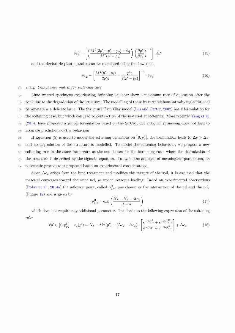
The use of the sigmoid equation appears very appropriate to model the degradation experienced at yield257
by lime treated materials. For both concentrations in lime, there is a very good agreement between the258
experimental results and the model. The degradation is initiated at the right effective mean stress and with259
the correct rate, and both sets converge toward the correct normal compression line.260
20
0 500 1000 1500 2000
p′ (kPa)
1.35
1.40
1.45
1.50
1.55
1.60
Specificvolumev(−
)
ncld
nclr
[CaO]=0.0 %
[CaO]=0.5 %
[CaO]=1.0 %
Simulation
Figure 14: Validation of the formulation on 0.5% and 1% lime treated specimens – ncld: normal compression line of the
untreated state, nclr: normal compression line of the residual state.
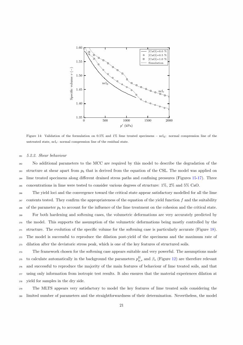
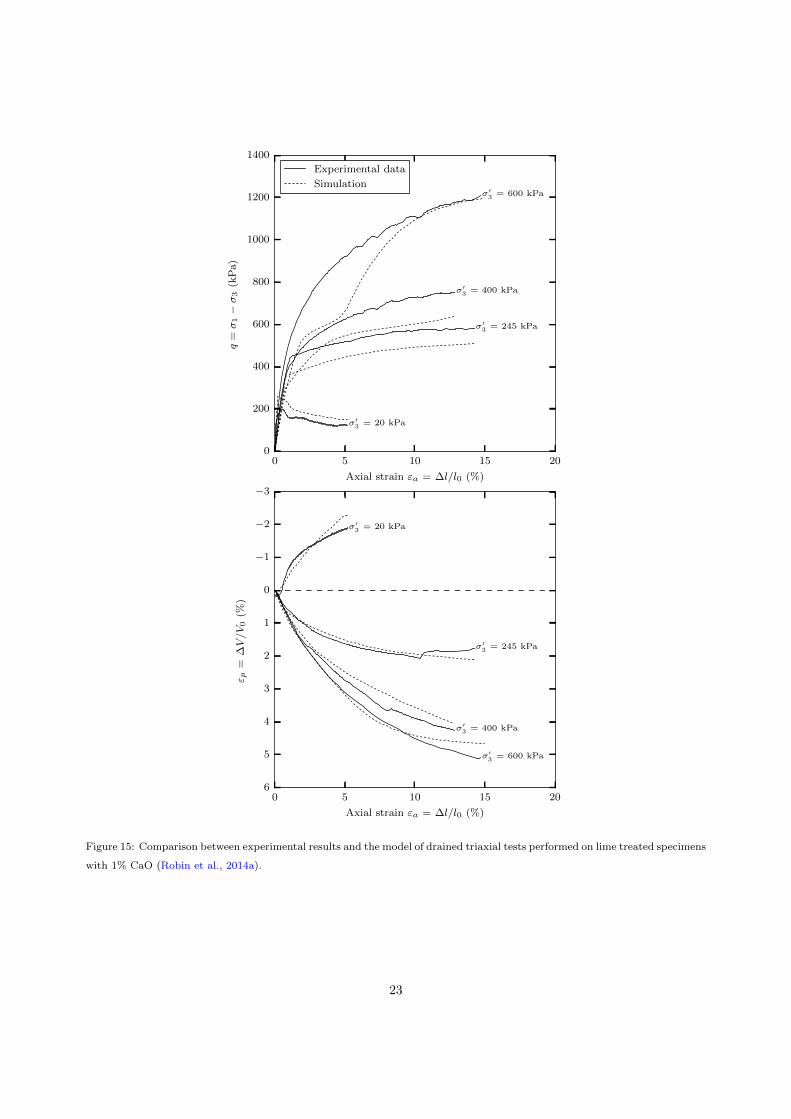
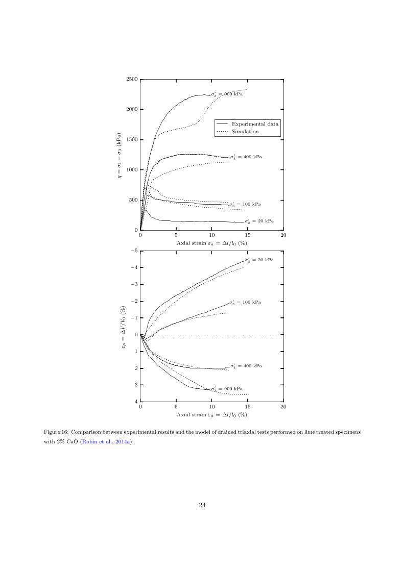
5.2.2. Shear behaviour261
No additional parameters to the MCC are required by this model to describe the degradation of the262
structure at shear apart from pb that is derived from the equation of the CSL. The model was applied on263
lime treated specimens along different drained stress paths and confining pressures (Figures 15-17). Three264
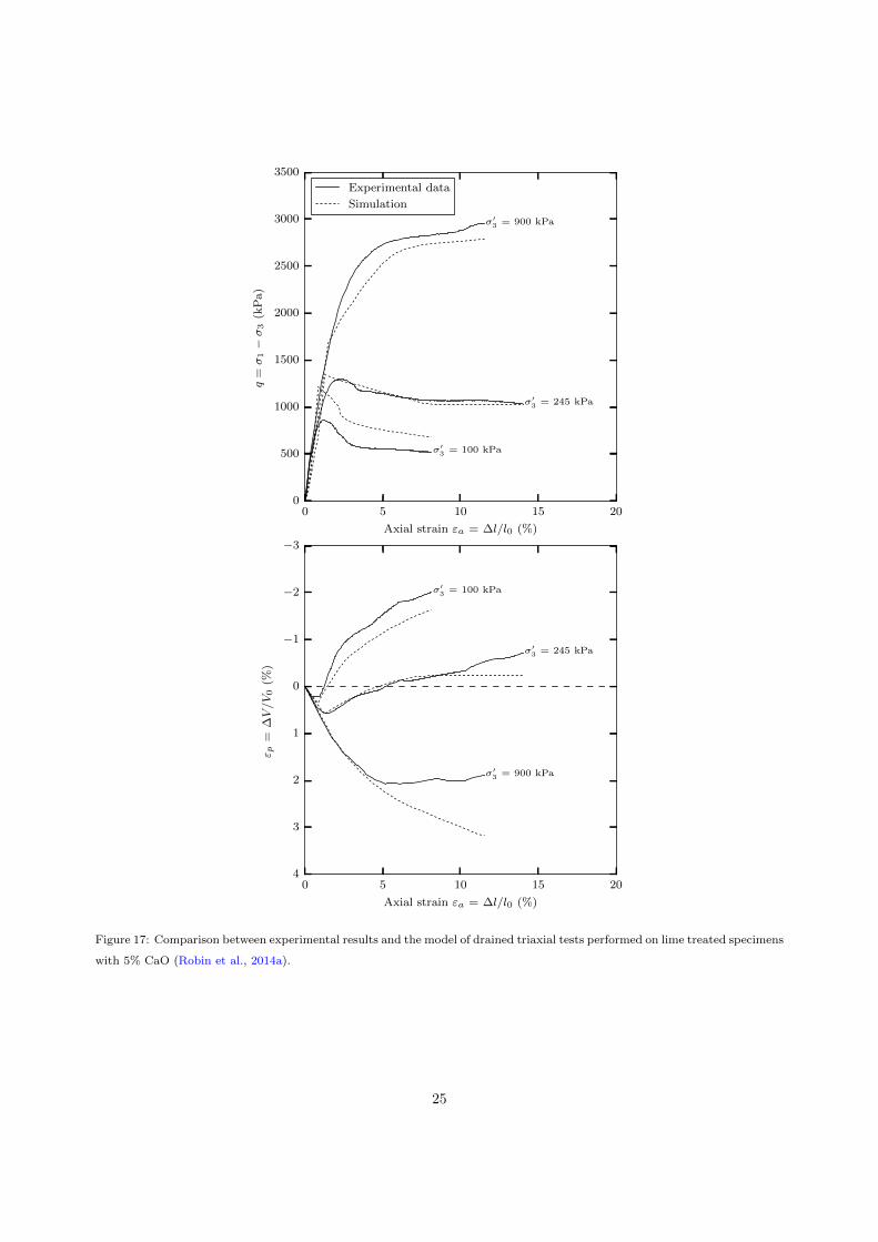
concentrations in lime were tested to consider various degrees of structure: 1%, 2% and 5% CaO.265
The yield loci and the convergence toward the critical state appear satisfactory modelled for all the lime266
contents tested. They confirm the appropriateness of the equation of the yield function f and the suitability267
of the parameter pb to account for the influence of the lime treatment on the cohesion and the critical state.268
For both hardening and softening cases, the volumetric deformations are very accurately predicted by269
the model. This supports the assumption of the volumetric deformations being mostly controlled by the270
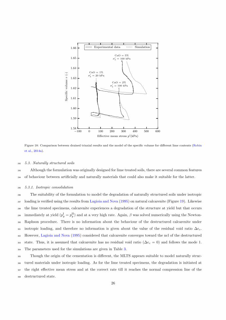
structure. The evolution of the specific volume for the softening case is particularly accurate (Figure 18).271
The model is successful to reproduce the dilation post-yield of the specimens and the maximum rate of272
dilation after the deviatoric stress peak, which is one of the key features of structured soils.273
The framework chosen for the softening case appears suitable and very powerful. The assumptions made274
to calculate automatically in the background the parameters pIIy,s and βs (Figure 12) are therefore relevant275
and successful to reproduce the majority of the main features of behaviour of lime treated soils, and that276
using only information from isotropic test results. It also ensures that the material experiences dilation at277
yield for samples in the dry side.278
The MLTS appears very satisfactory to model the key features of lime treated soils considering the279
limited number of parameters and the straightforwardness of their determination. Nevertheless, the model280
21

tends to deviate from the experimental results during the post-yield stage before converging back toward281
the critical state at high axial strains for some samples subjected to a high preconsolidation pressure (600282
kPa in Figure 15, 900 kPa in Figure 16). In this model, potentials f and g are associated and hardening283
is controlled by the plastic volumetric deformations εpp only (f(σ, εpp)). This has for consequences to reflect284
the degradation of the structure on the deviatoric stress. However, lime treated specimens experiencing285
hardening do not show any sign of this phenomenon for any of the concentrations tested. This might come286
from the fact that the contribution of εpq was neglected in this model, and/or that the ‘amount’ of structure287
is too low to significantly affect the stresses.288
For samples in the dry side, the model predicts larger values for the yield loci than what is experimentally289
observed. One of the known limitations of the MCC is that it overestimates the values in such situation;290
the fact that we extended the yield function in the tensile domain with pb amplifies this feature.291
22
0 5 10 15 20
Axial strain εa = ∆l/l0 (%)
0
200
400
600
800
1000
1200
1400
q=
σ1−
σ3(kPa)
σ′3 = 20 kPa
σ′3 = 245 kPa
σ′3 = 400 kPa
σ′3 = 600 kPa
Experimental data
Simulation
0 5 10 15 20
Axial strain εa = ∆l/l0 (%)
−3
−2
−1
0
1
2
3
4
5
6
ε p=
∆V/V0(%
)
σ′3 = 20 kPa
σ′3 = 245 kPa
σ′3 = 400 kPa
σ′3 = 600 kPa
Figure 15: Comparison between experimental results and the model of drained triaxial tests performed on lime treated specimens
with 1% CaO (Robin et al., 2014a).
23
0 5 10 15 20
Axial strain εa = ∆l/l0 (%)
0
500
1000
1500
2000
2500
q=
σ1−
σ3(kPa)
σ′3 = 20 kPa
σ′3 = 100 kPa
σ′3 = 400 kPa
σ′3 = 900 kPa
Experimental data
Simulation
0 5 10 15 20
Axial strain εa = ∆l/l0 (%)
−5
−4
−3
−2
−1
0
1
2
3
4
ε p=
∆V/V0(%
)
σ′3 = 20 kPa
σ′3 = 100 kPa
σ′3 = 400 kPa
σ′3 = 900 kPa
Figure 16: Comparison between experimental results and the model of drained triaxial tests performed on lime treated specimens
with 2% CaO (Robin et al., 2014a).
24
0 5 10 15 20
Axial strain εa = ∆l/l0 (%)
0
500
1000
1500
2000
2500
3000
3500
q=
σ1−
σ3(kPa)
σ′3 = 100 kPa
σ′3 = 245 kPa
σ′3 = 900 kPa
Experimental data
Simulation
0 5 10 15 20
Axial strain εa = ∆l/l0 (%)
−3
−2
−1
0
1
2
3
4
ε p=
∆V/V0(%
)
σ′3 = 100 kPa
σ′3 = 245 kPa
σ′3 = 900 kPa
Figure 17: Comparison between experimental results and the model of drained triaxial tests performed on lime treated specimens
with 5% CaO (Robin et al., 2014a).
25
−100 0 100 200 300 400 500 600
Effective mean stress p′(kPa)
1.58
1.59
1.60
1.61
1.62
1.63
1.64
1.65
1.66
Specificvolumev(-) CaO = 1%
σ′3 = 20 kPa
CaO = 2%
σ′3 = 100 kPa
CaO = 5%
σ′3 = 100 kPa
Experimental data Simulation
Figure 18: Comparison between drained triaxial results and the model of the specific volume for different lime contents (Robin
et al., 2014a).
5.3. Naturally structured soils292
Although the formulation was originally designed for lime treated soils, there are several common features293
of behaviour between artificially and naturally materials that could also make it suitable for the latter.294
5.3.1. Isotropic consolidation295
The suitability of the formulation to model the degradation of naturally structured soils under isotropic296
loading is verified using the results from Lagioia and Nova (1995) on natural calcarenite (Figure 19). Likewise297
the lime treated specimens, calcarenite experiences a degradation of the structure at yield but that occurs298
immediately at yield (pIy = pIIy ) and at a very high rate. Again, β was solved numerically using the Newton-299
Raphson procedure. There is no information about the behaviour of the destructured calcarenite under300
isotropic loading, and therefore no information is given about the value of the residual void ratio ∆ec.301
However, Lagioia and Nova (1995) considered that calcarenite converges toward the ncl of the destructured302
state. Thus, it is assumed that calcarenite has no residual void ratio (∆ec = 0) and follows the mode 1.303
The parameters used for the simulations are given in Table 3.304
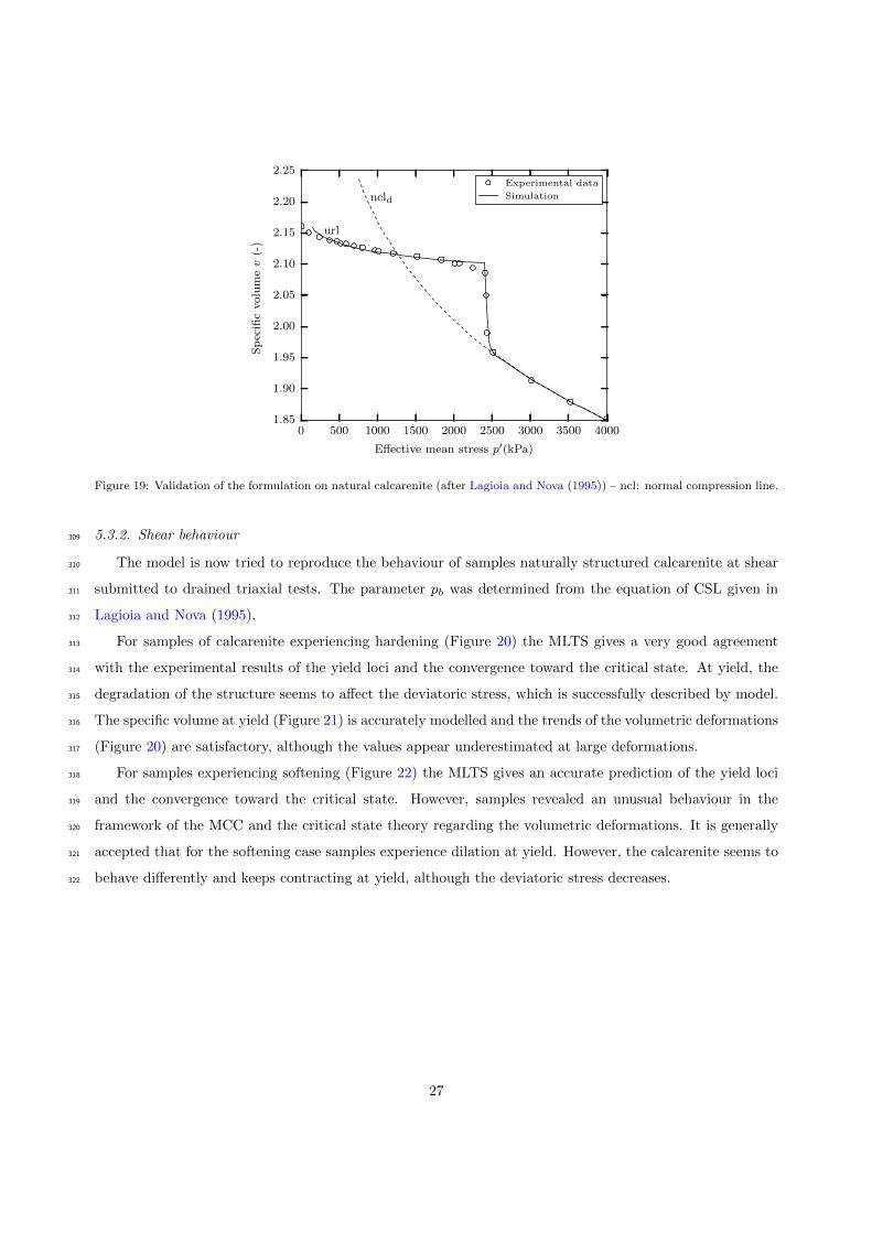
Though the origin of the cementation is different, the MLTS appears suitable to model naturally struc-305
tured materials under isotropic loading. As for the lime treated specimens, the degradation is initiated at306
the right effective mean stress and at the correct rate till it reaches the normal compression line of the307
destructured state.308
26
0 500 1000 1500 2000 2500 3000 3500 4000
Effective mean stress p′(kPa)
1.85
1.90
1.95
2.00
2.05
2.10
2.15
2.20
2.25
Specificvolumev(-)
url
ncld
Experimental data
Simulation
Figure 19: Validation of the formulation on natural calcarenite (after Lagioia and Nova (1995)) – ncl: normal compression line.
5.3.2. Shear behaviour309
The model is now tried to reproduce the behaviour of samples naturally structured calcarenite at shear310
submitted to drained triaxial tests. The parameter pb was determined from the equation of CSL given in311
Lagioia and Nova (1995).312
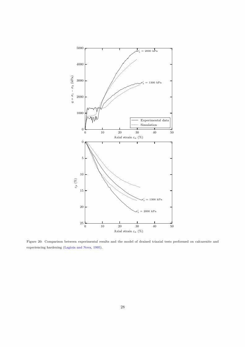
For samples of calcarenite experiencing hardening (Figure 20) the MLTS gives a very good agreement313
with the experimental results of the yield loci and the convergence toward the critical state. At yield, the314
degradation of the structure seems to affect the deviatoric stress, which is successfully described by model.315
The specific volume at yield (Figure 21) is accurately modelled and the trends of the volumetric deformations316
(Figure 20) are satisfactory, although the values appear underestimated at large deformations.317
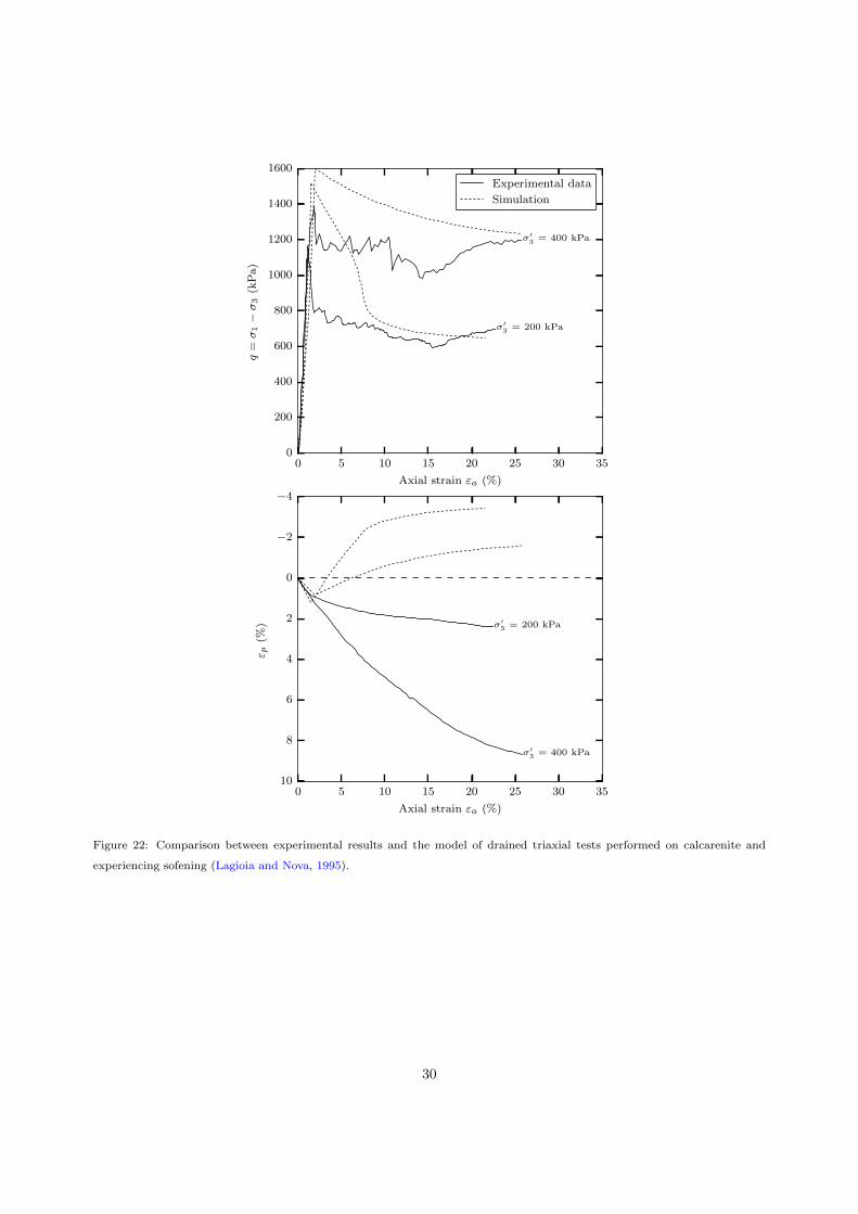
For samples experiencing softening (Figure 22) the MLTS gives an accurate prediction of the yield loci318
and the convergence toward the critical state. However, samples revealed an unusual behaviour in the319
framework of the MCC and the critical state theory regarding the volumetric deformations. It is generally320
accepted that for the softening case samples experience dilation at yield. However, the calcarenite seems to321
behave differently and keeps contracting at yield, although the deviatoric stress decreases.322
27
0 10 20 30 40 50
Axial strain εa (%)
0
1000
2000
3000
4000
5000
q=
σ1−
σ3(kPa)
σ′3 = 1300 kPa
σ′3 = 2000 kPa
Experimental data
Simulation
0 10 20 30 40 50
Axial strain εa (%)
0
5
10
15
20
25
ε p(%
)
σ′3 = 1300 kPa
σ′3 = 2000 kPa
Figure 20: Comparison between experimental results and the model of drained triaxial tests performed on calcarenite and
experiencing hardening (Lagioia and Nova, 1995).
28

0 1000 2000 3000 4000 5000
Effective mean stress p′(kPa)
1.5
1.6
1.7
1.8
1.9
2.0
2.1
2.2
Specificvolumev(-)
1300 kPa
2000 kPa
Experimental data Simulation
Figure 21: Comparison between the experimental results and the model for the specific volume (Lagioia and Nova, 1995)
29
0 5 10 15 20 25 30 35
Axial strain εa (%)
0
200
400
600
800
1000
1200
1400
1600
q=
σ1−
σ3(kPa)
σ′3 = 200 kPa
σ′3 = 400 kPa
Experimental data
Simulation
0 5 10 15 20 25 30 35
Axial strain εa (%)
−4
−2
0
2
4
6
8
10
ε p(%
) σ′3 = 200 kPa
σ′3 = 400 kPa
Figure 22: Comparison between experimental results and the model of drained triaxial tests performed on calcarenite and
experiencing sofening (Lagioia and Nova, 1995).
30
5.4. Discussion: influence of the initial void ratio on the degradation mode323
The MLTS can successfully reproduce a large number of features of both lime treated soils and naturally324
structured soils. However, the model deviates from the experimental results for 1) lime treated specimens325
subjected to high preconsolidation pressures experiencing hardening, and 2) samples of calcarenite experi-326
encing softening. In this section, we propose a hypothesis to explain these limitations using the initial void327
ratio of the material.328
During the early post-yield stage, the degradation of the structure seems to affect the stress:strain329
response for samples of calcarenite experiencing hardening, but not for the lime treated specimens. Fur-330
thermore, for the softening case, lime treated specimens experience dilation, as predicted by the critical331
state theory, but this is not the case for the samples of calcarenite, which experience contraction despite the332
decrease of deviatoric stress at yield.333
For the calcarenite, the initial additional void ratio at yield ∆ei and the range of stresses are similar to334
those measured on lime treated soils with 5% CaO. The only difference between the two materials lies in335
the initial specific volume (around 1.6 for the lime treated specimens and 2.2 for the calcarenite). When336
the calcarenite starts yielding, the structure is rapidly degraded due to the brittleness of the material.337
Lagioia and Nova (1995) stated that some softening could take place under isotropic loading, and explained338
that the plateau of the deviatoric stress is associated with debonding. However, what was interpreted as339
softening under isotropic loading is more likely to be collapse since the specific volume decreases during the340
destructuration. Once the particles are released from the cementation, they immediately collapse and start341
filling the voids as the axial deformation increases. During this stage, there is no effective friction inside the342
material and therefore no additional deviatoric stress is necessary to increase the axial deformation. The343
effective friction is restored once the particles are close enough and the porosity is significantly reduced,344
which leads to an increase of the deviatoric stress followed by convergence toward the critical state. This345
mechanism also explains why samples experiencing softening do not have a dilatant behaviour at yield as346
predicted by the critical state theory. The dilation process is the direct result of the interlocking of the347
particles; in the case of the calcarenite, the fast degradation of the structure leads to the collapsing of the348
particles and therefore to the contraction of the sample. Although the deviatoric stress decreases at yield,349
since there is no interlocking of the particles, there is no dilation of the sample.350
For the lime treated specimens of this study, the initial conditions were chosen to match those used351
on-site and obtained from the Proctor compaction test (Robin et al., 2014a). In these conditions, the void352
ratio is too low to generate a noticeable collapse in the material, and the destructuration is a slower process.353
The degradation of the structure takes place but particles are already in contact, which maintains a friction354
between them and leads to increase in the deviatoric stress with the axial deformation. Therefore, the355
degradation of the structure is not observed directly on the stress:strain response. If the conditions imply356
strain softening, interlocking happens and therefore dilation, which is observed on the experimental results357
31
and properly reproduced by the MLTS.358
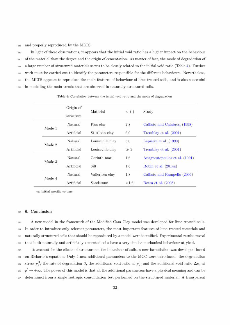
In light of these observations, it appears that the initial void ratio has a higher impact on the behaviour359
of the material than the degree and the origin of cementation. As matter of fact, the mode of degradation of360
a large number of structured materials seems to be closely related to the initial void ratio (Table 4). Further361
work must be carried out to identify the parameters responsible for the different behaviours. Nevertheless,362
the MLTS appears to reproduce the main features of behaviour of lime treated soils, and is also successful363
in modelling the main trends that are observed in naturally structured soils.364
Table 4: Correlation between the initial void ratio and the mode of degradation
Origin ofMaterial vi (-) Study
structure
Mode 1Natural Pisa clay 2.8 Callisto and Calabresi (1998)
Artificial St-Alban clay 6.0 Tremblay et al. (2001)
Mode 2Natural Louiseville clay 3.0 Lapierre et al. (1990)
Artificial Louiseville clay � 3 Tremblay et al. (2001)
Mode 3Natural Corinth marl 1.6 Anagnostopoulos et al. (1991)
Artificial Silt 1.6 Robin et al. (2014a)
Mode 4Natural Vallericca clay 1.8 Callisto and Rampello (2004)
Artificial Sandstone <1.6 Rotta et al. (2003)
vi: initial specific volume.
6. Conclusion365
A new model in the framework of the Modified Cam Clay model was developed for lime treated soils.366
In order to introduce only relevant parameters, the most important features of lime treated materials and367
naturally structured soils that should be reproduced by a model were identified. Experimental results reveal368
that both naturally and artificially cemented soils have a very similar mechanical behaviour at yield.369
To account for the effects of structure on the behaviour of soils, a new formulation was developed based370
on Richards’s equation. Only 4 new additional parameters to the MCC were introduced: the degradation371
stress pIIy , the rate of degradation β, the additional void ratio at pIy, and the additional void ratio ∆ec at372
p′ → +∞. The power of this model is that all the additional parameters have a physical meaning and can be373
determined from a single isotropic consolidation test performed on the structured material. A transparent374
32
and powerful procedure was developed for the softening rule. The two parameters required by the sigmoid375
function to model the degradation are automatically determined from the 4 parameters obtained from the376
isotropic tests.377
The model was applied for lime treated soils and naturally structured samples of calcarenite. The378
formulation is in good agreement with the experimental results and the main trends are properly reproduced.379
The formulation proposed as softening rule is successful to model the dilation observed on lime treated380
samples at yield and the maximum rate of dilation after the peak, one of the most representative features381
of structured soils. However, the results on the calcarenite have risen interesting considerations for the382
modelling of the structured materials in general, naturally or artificially.383
The initial porosity appeared to be the key parameter controlling the influence of the mode of structure384
degradation on the mechanical behaviour of lime treated specimens and the calcarenite. Once the material385
starts yielding the degradation of the bonding structure takes place, and therefore the release of the particles.386
Depending on the initial void ratio, the material can either experience dilation (particles are in contact and387
expand due to the interlocking) or collapse until particles start interacting again. This can lead to reduction388
of volume even for heavily over consolidated samples.389
Further work must be carried out to develop a model capable of accounting for the influence of the initial390
void ratio on the post-yield behaviour.391
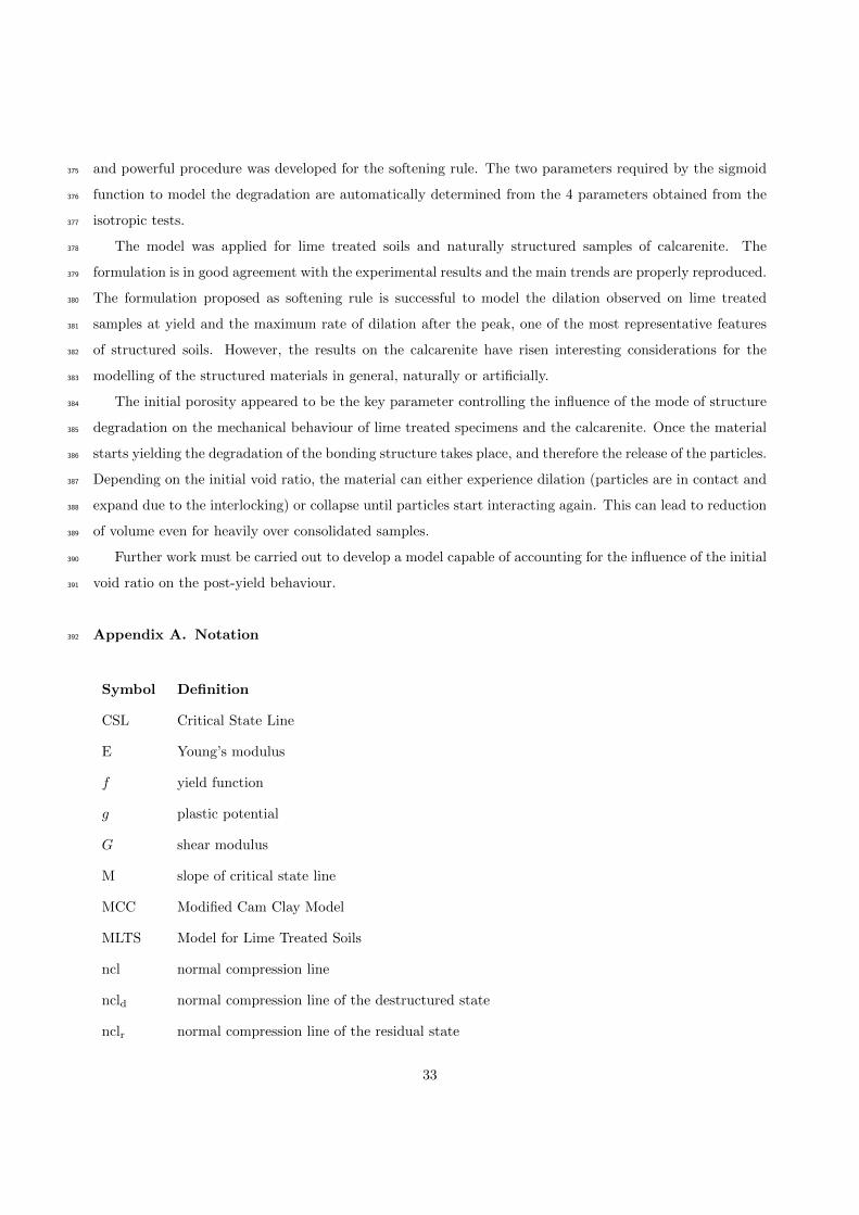
Appendix A. Notation392
Symbol Definition
CSL Critical State Line
E Young’s modulus
f yield function
g plastic potential
G shear modulus
M slope of critical state line
MCC Modified Cam Clay Model
MLTS Model for Lime Treated Soils
ncl normal compression line
ncld normal compression line of the destructured state
nclr normal compression line of the residual state
33
Symbol Definition
nclmcc normal compression line of modified Cam Clay model
Nλ specific volume at p′ = 1 kPa
p′ effective mean stress
pb tensile stress
pIy primary yield stress
pIIy degradation stress
pIIy,s degradation stress for softening case
q deviatoric stress
url unloading-reloading line
v specific volume
vs specific volume for the structured soil
α parameter of bijection for softening case
β rate of degradation
βs rate of degradation for softening case
β0 rate of degradation for monotonic decreasing function vs
∆ec residual additional void ratio at p′ → +∞
∆ei initial additional void ratio at p′ = pIy
εp, εep, ε
pp total, elastic, and plastic volumetric strains
εq, εeq, ε
pq total, elastic, and plastic deviatoric strains
κ elastic stiffness parameter for changes in effective mean stress
λ plastic stiffness parameter for changes in effective mean stress
ξ gradient of the curve (v : p′) at p′ = pIIy
σ1, σ3 axial, radial stress
34
7. References393
Ahnberg, H., 2007. On yield stresses and the influence of curing stresses on stress paths and strength measured in triaxial394
testing of stabilized soils. Canadian geotechnical journal 44 (1), 54–66.395
Anagnostopoulos, a. G., Kalteziotis, N., Tsiambaos, G. K., Kavvadas, M., 1991. Geotechnical properties of the Corinth Canal396
marls. Geotechnical and Geological Engineering 9 (1), 1–26.397
Aversa, S., 1991. Mechanical behaviour of soft rocks: some remarks. In: Proc. of the Workshop on ”Experimental characteri-398
zation and modelling of soils and soft”. Vol. 98. pp. 191–223.399
Balasubramaniam, A., Buessucesco, B., Oh, Y.-N. E., Bolton, M. W., Bergado, D., Lorenzo, G., 2005. Strength degradation400
and critical state seeking behaviour of lime treated soft clay. In: International Conference on Deep Mixing-Best Practice401
and Recent Advances. Vol. 1. Stockholm, pp. 35–40.402
Baudet, B., Stallebrass, S., 2004. A constitutive model for structured clays. Geotechnique 54 (4), 269–278.403
Brandl, H., 1981. Alteration of soil parameters by stabilization with lime. In: 10th International Conference on Soil Mechanics404
and Foundation Engineering. Stockholm, pp. 587–594.405
Burland, J. B., 1990. On the compressibility and shear strength of natural clays. Geotechnique 40 (3), 329–378.406
Burland, J. B., Rampello, S., Georgiannou, V. N., Calabresi, G., 1996. A laboratory study of the strength of four stiff clays.407
Geotechnique 46 (3), 491–514.408
Callisto, L., Calabresi, G., 1998. Mechanical behaviour of a natural soft clay. Geotechnique 48 (4), 495–513.409
Callisto, L., Rampello, S., 2004. An interpretation of structural degradation for three natural clays. Canadian Geotechnical410
Journal 41 (3), 392–407.411
Consoli, N. C., Lopes, L. d. S., Prietto, P. D. M., Festugato, L., Cruz, R. C., 2011. Variables Controlling Stiffness and Strength412
of Lime-Stabilized Soils. Journal of Geotechnical and Geoenvironmental Engineering 137 (6), 628–632.413
Corless, R. M., Gonnet, G. H., Hare, D. E. G., Jeffrey, D. J., Knuth, D. E., 1996. On the Lambert W Function. Advances in414
Computational Mathematics 5, 329–359.415
Cotecchia, F., Chandler, R. J., 2000. A general framework for the mechanical behaviour of clays. Geotechnique 50 (4), 431–447.416
Cuisinier, O., Auriol, J.-C., Le Borgne, T., Deneele, D., 2011. Microstructure and hydraulic conductivity of a compacted417
lime-treated soil. Engineering Geology 123 (3), 187–193.418
Cuisinier, O., Masrouri, F., Pelletier, M., Villieras, F., Mosser-Ruck, R., 2008. Microstructure of a compacted soil submitted419
to an alkaline PLUME. Applied Clay Science 40 (1-4), 159–170.420
Flora, A., Lirer, S., Amorosi, A., Elia, G., 2006. Experimental observations and theoretical interpretation of the mechanical421
behaviour of a grouted pyroclastic silty sand. In: Proc. VI European Conference on Numerical Methods in Geotechnical422
Engineering, NUMGE 06. Graz, Austria.423
Gens, A., Nova, R., 1993. Conceptual bases for a constitutive model for bonded soils and weak rocks. Geotechnical engineering424
of hard soils-soft rocks 1 (1), 485–494.425
Horpibulsuk, S., Liu, M. D., Liyanapathirana, D. S., Suebsuk, J., 2010. Behaviour of cemented clay simulated via the theoretical426
framework of the Structured Cam Clay model. Computers and Geotechnics 37 (1-2), 1–9.427
Kavvadas, M., Amorosi, A., 2000. A constitutive model for structured soils. Geotechnique 50 (3), 263–273.428
Lagioia, R., Nova, R., 1995. An experimental and theoretical study of the behaviour of a calcarenite in triaxial compression.429
Geotechnique 45 (4), 633–648.430
Lapierre, C., Leroueil, S., Locat, J., 1990. Mercury intrusion and permeability of Louiseville clay. Canadian Geotechnical431
Journal 27 (6), 761–773.432
Leroueil, S., Vaughan, P. R., 1990. The general and congruent effects of structure in natural soils and weak rocks. Geotechnique433
40 (3), 467–488.434
Little, D. N., 1995. Stabilization of pavement subgrades and base courses with lime. Kendall Hunt Pub Co.435
35
Liu, M. D., Carter, J. P., 2002. A structured Cam Clay model. Canadian Geotechnical Journal 39 (6), 1313–1332.436
Liu, M. D., Carter, J. P., 2003. Volumetric Deformation of Natural Clays. International Journal of Geomechanics 3 (2), 236–252.437
Maccarini, M., 1987. Laboratory studies for a weakly bonded artificial soil. Ph.D. thesis, Imperial College London (University438
of London).439
Malandraki, V., Toll, D. G., 2001. Triaxial Tests on Weakly Bonded Soil with Changes in Stress Path. Journal of Geotechnical440
and Geoenvironmental Engineering 127 (3), 282–291.441
Muir Wood, D., 2004. Geotechnical modelling. Vol. Applied Ge. CRC Press.442
Nguyen, L. D., Fatahi, B., Khabbaz, H., 2014. A constitutive model for cemented clays capturing cementation degradation.443
International Journal of Plasticity 56, 1–18.444
Nova, R., Castellanza, R., Tamagnini, C., 2003. A constitutive model for bonded geomaterials subject to mechanical and/or445
chemical degradation. International journal for numerical and analytical methods in geomechanics 27 (9), 705–732.446
Oliveira, P. V., 2013. Effect of Stress Level and Binder Composition on Secondary Compression of an Artificially Stabilized447
Soil. Journal of Geotechnical and Geoenvironmental Engineering 139 (5), 810–820.448
Rampello, S., Callisto, L., 1998. A study on the subsoil of the Tower of Pisa based on results from standard and high-quality449
samples. Canadian Geotechnical Journal 35 (6), 1074–1092.450
Richards, F., 1959. A flexible growth function for empirical use. Journal of experimental Botany 10 (29), 290–300.451
Robin, V., Cuisinier, O., Masrouri, F., Javadi, A. A., 2014a. Chemo-mechanical modelling of lime treated soils. Applied Clay452
Science 95, 211–219.453
Robin, V., Javadi, A. A., Cuisinier, O., Masrouri, F., 2014b. A new formulation to model the degradation in structured soils.454
In: 8th European Conference on Numerical Methods in Geotechnical Engineering. Delft, pp. 97–102.455
Roscoe, K. H., Burland, J. B., 1968. On the generalized stress-strain behaviour of wet clay. Engineering Plasticity, 535–609.456
Rotta, G. V., Consoli, N. C., Prietto, P. D. M., Coop, M. R., Graham, J., 2003. Isotropic yielding in an artificially cemented457
soil cured under stress. Geotechnique 53 (5), 493–501.458
Rouainia, M., Muir wood, D., 2000. A kinematic hardening constitutive model for natural clays with loss of structure.459
Suebsuk, J., Horpibulsuk, S., Liu, M. D., 2010. Modified Structured Cam Clay: A generalised critical state model for destruc-460
tured, naturally structured and artificially structured clays. Computers and Geotechnics 37 (7-8), 956–968.461
Suebsuk, J., Horpibulsuk, S., Liu, M. D., 2011. A critical state model for overconsolidated structured clays. Computers and462
Geotechnics 38 (5), 648–658.463
Tremblay, H., Leroueil, S., Locat, J., 2001. Mechanical improvement and vertical yield stress prediction of clayey soils from464
eastern Canada treated with lime or cement. Canadian Geotechnical Journal 38 (3), 567–579.465
Vatsala, A., Nova, R., Srinivasa Murthy, B. R., 2001. Elastoplastic Model for Cemented Soils. Journal of Geotechnical and466
Geoenvironmental Engineering 127 (8), 679–687.467
Wissa, A. E., Ladd, C. C., Lambe, T. W., 1965. Effective stress strength parameters of stabilized soils. In: International468
conference on soil mechanics and foundation engineering. Montreal, pp. 412–416.469
Yang, C., Carter, J. P., Sheng, D., 2014. Description of compression behaviour of structured soils and its application 933 (July470
2013), 921–933.471
Yong, R., Nagaraj, T., 1977. Investigation of fabric and compressibility of a sensitive clay. In: Proceedings of the International472
Symposium on Soft Clay, Asian Institute of Technology. pp. 327–333.473
Zytynski, M., Randolph, M., Nova, R., Wroth, C., 1978. On modelling the unloading-reloading behaviour of soils. International474
Journal for Numerical and Analytical Methods in Geomechanics 2 (1), 87–93.475
36


