
Hidden Markov Models
Machine Learning CSx824/ECEx242
Bert Huang Virginia Tech
Outline
• Hidden Markov models (HMMs)
• Forward-backward for HMMs
• Baum-Welch learning (expectation maximization)
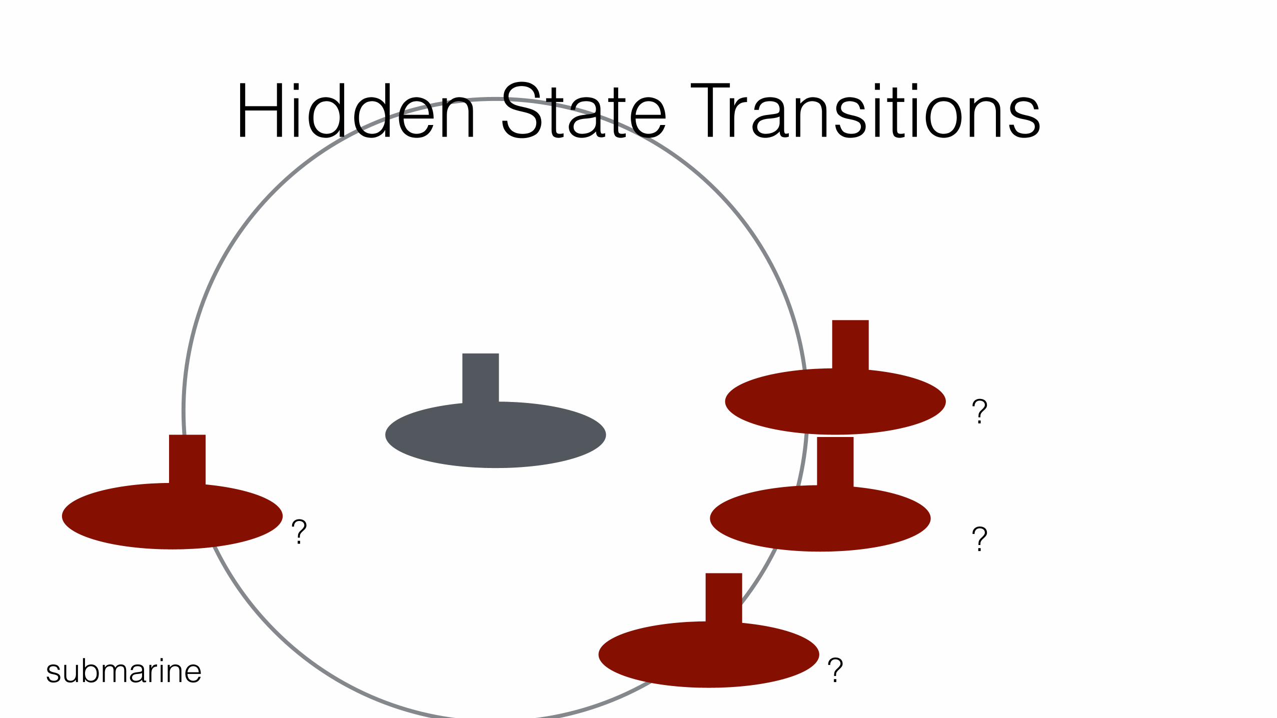
Hidden State Transitions
submarine
?
?
?
?

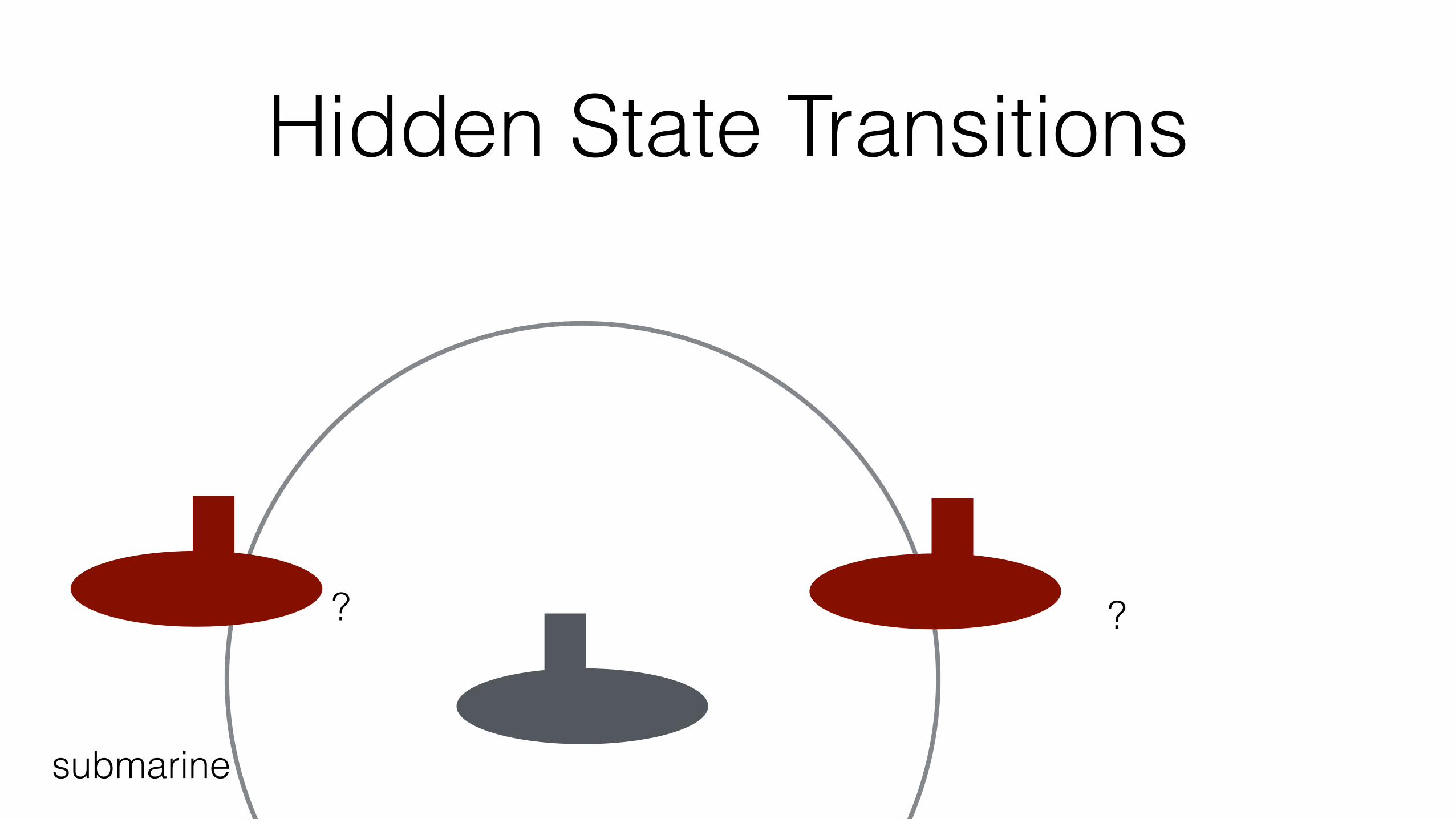
Hidden State Transitions
submarine
?
?
?
?
Hidden State Transitions
submarine
??
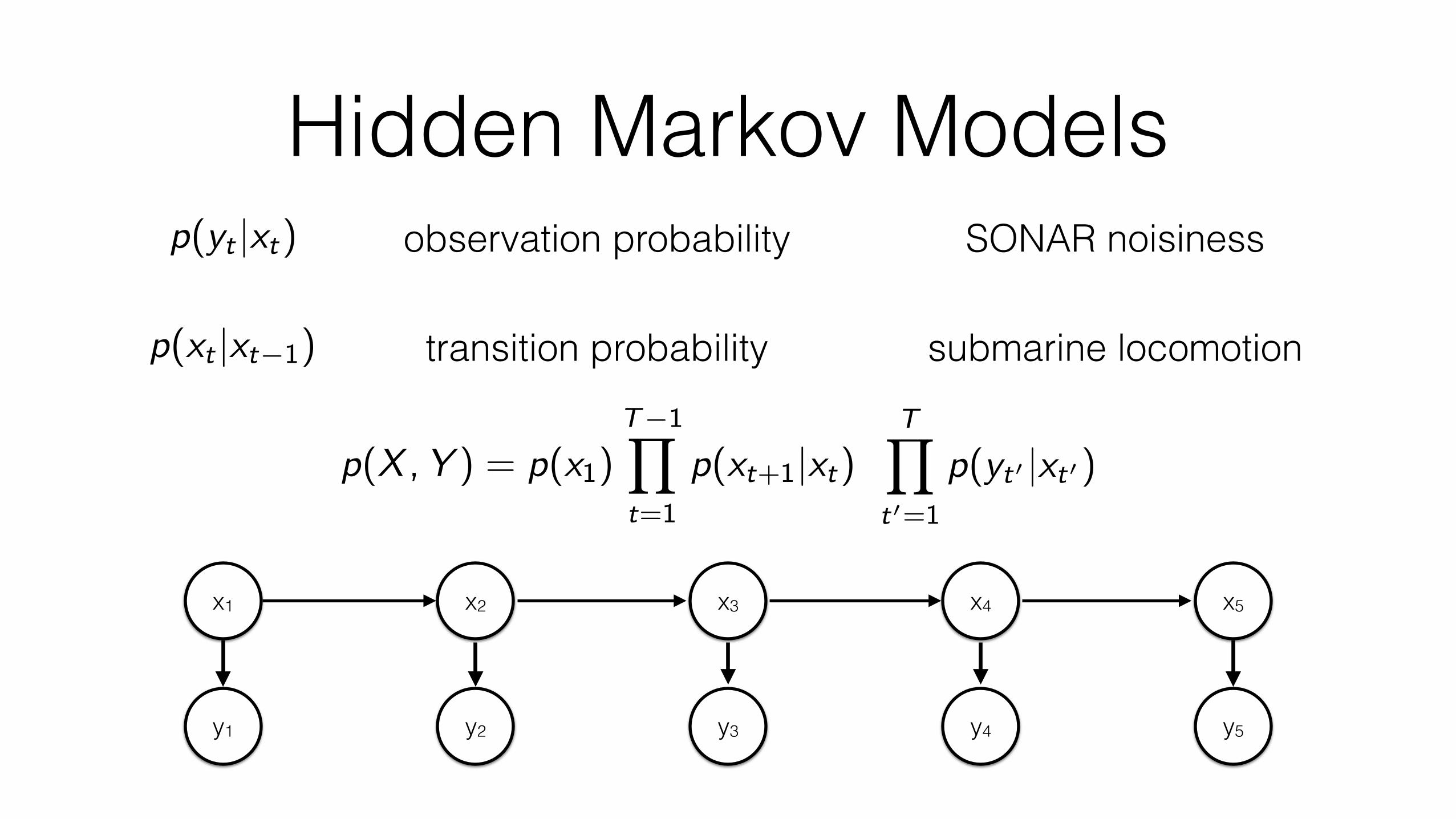
Hidden Markov Modelsp(yt |xt)
p(xt |xt�1)
observation probability
transition probability submarine locomotion
SONAR noisiness
p(X ,Y ) = p(x1)T�1Y
t=1
p(xt+1|xt)TY
t0=1
p(yt0 |xt0)
x1 x2 x3 x4 x5
y1 y2 y3 y4 y5

Hidden State Inferencep(X |Y ) p(xt |Y )
↵t(xt) = p(xt , y1, ... , yt) �t(xt) = p(yt+1, ... , yT |xt)
↵t(xt)�t(xt) = p(xt , y1, ... , yt)p(yt+1, ... , yT |xt) = p(xt ,Y ) / p(xt |Y )
normalize to get conditional probability
note: not the same as p(x1, ... , xT ,Y )
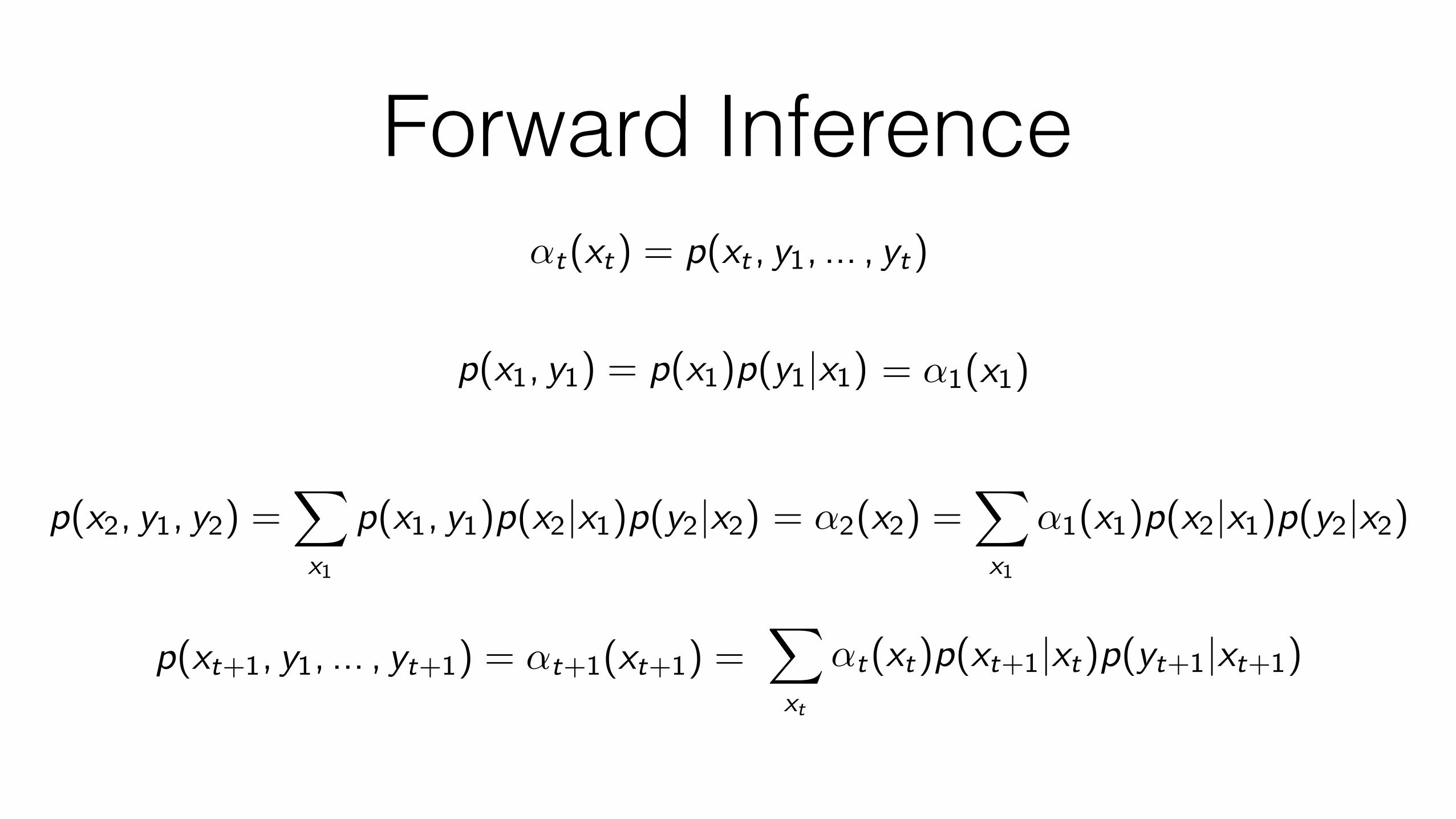
Forward Inference
p(x1, y1) = p(x1)p(y1|x1)
p(x2, y1, y2) =X
x1
p(x1, y1)p(x2|x1)p(y2|x2) = ↵2(x2) =X
x1
↵1(x1)p(x2|x1)p(y2|x2)
= ↵1(x1)
↵t(xt) = p(xt , y1, ... , yt)
p(xt+1, y1, ... , yt+1) = ↵t+1(xt+1) =X
x
t
↵t
(xt
)p(xt+1|xt)p(yt+1|xt+1)

Backward Inference�t(xt) = p(yt+1, ... , yT |xt)
p({}|xT ) = 1 = �T (xT )
�t�1(xt�1) = p(yt , ... , yT |xt�1) =X
x
t
p(xt
|xt�1)p(yt , yt+1, ... , yT |xt)
=X
x
t
p(xt
|xt�1)p(yt |xt)p(yt+1, ... , yT |xt)
=X
x
t
p(xt
|xt�1)p(yt |xt)�t
(xt
)
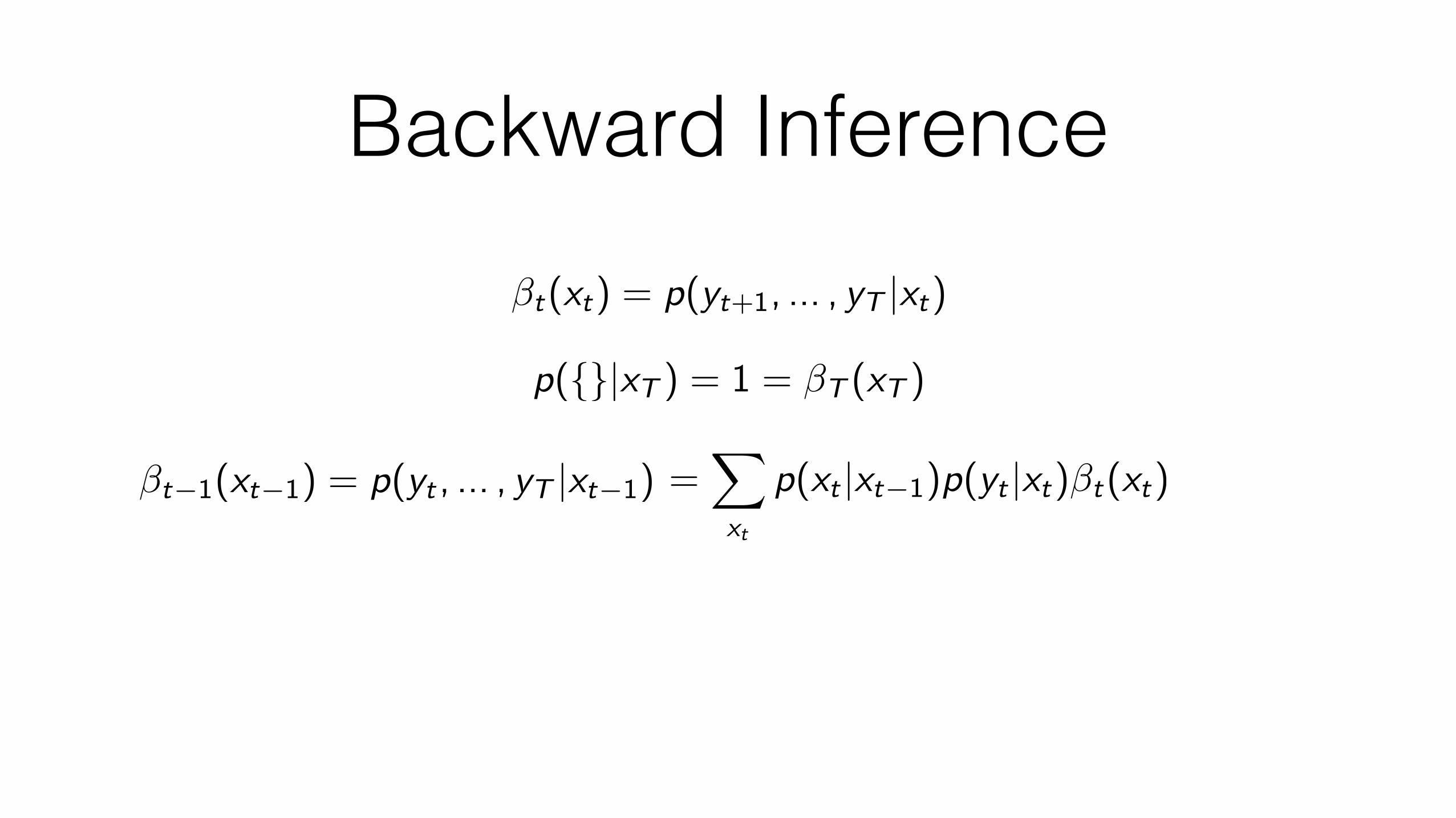
Backward Inference�t(xt) = p(yt+1, ... , yT |xt)
p({}|xT ) = 1 = �T (xT )
�t�1(xt�1) = p(yt , ... , yT |xt�1) =X
x
t
p(xt
|xt�1)p(yt |xt)�t
(xt
)
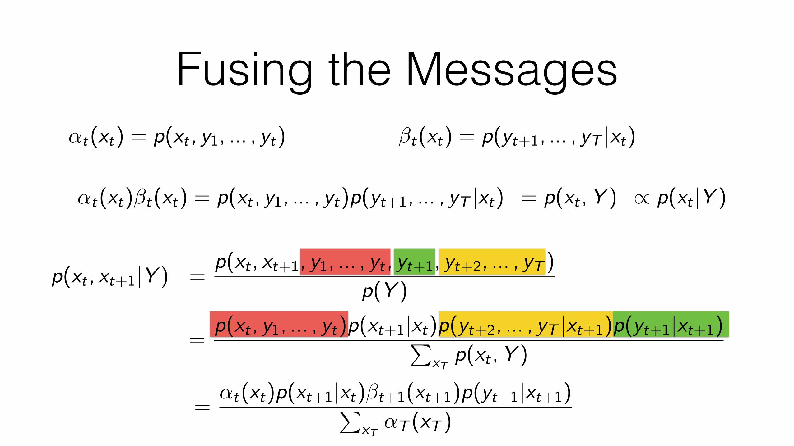
Fusing the Messages↵t(xt) = p(xt , y1, ... , yt) �t(xt) = p(yt+1, ... , yT |xt)
↵t(xt)�t(xt) = p(xt , y1, ... , yt)p(yt+1, ... , yT |xt) = p(xt ,Y ) / p(xt |Y )
p(xt , xt+1|Y )
=p(x
t
, y1, ... , yt)p(xt+1|xt)p(yt+2, ... , yT |xt+1)p(yt+1|xt+1)Px
T
p(xt
,Y )
=p(xt , xt+1, y1, ... , yt , yt+1, yt+2, ... , yT )
p(Y )
=↵t
(xt
)p(xt+1|xt)�t+1(xt+1)p(yt+1|xt+1)P
x
T
↵T
(xT
)
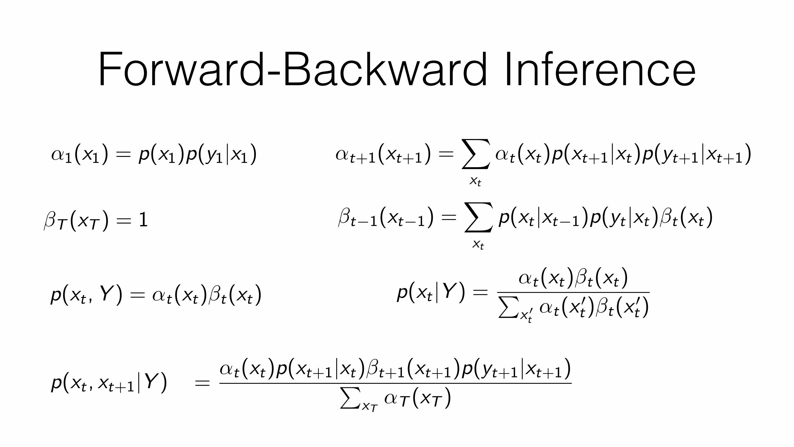
Forward-Backward Inference↵1(x1) = p(x1)p(y1|x1) ↵
t+1(xt+1) =X
x
t
↵t
(xt
)p(xt+1|xt)p(yt+1|xt+1)
�T (xT ) = 1 �t�1(xt�1) =
X
x
t
p(xt
|xt�1)p(yt |xt)�t
(xt
)
p(xt ,Y ) = ↵t(xt)�t(xt) p(xt
|Y ) =↵t
(xt
)�t
(xt
)Px
0t
↵t
(x 0t
)�t
(x 0t
)
p(xt , xt+1|Y ) =↵t
(xt
)p(xt+1|xt)�t+1(xt+1)p(yt+1|xt+1)P
x
T
↵T
(xT
)

Normalization
↵̃t
(xt
) =↵t
(xt
)Px
0t
↵t
(x 0t
)�̃t
(xt
) =�t
(xt
)Px
0t
�t
(x 0t
)
To avoid underflow, re-normalize at each time step
Exercise: why is this okay?
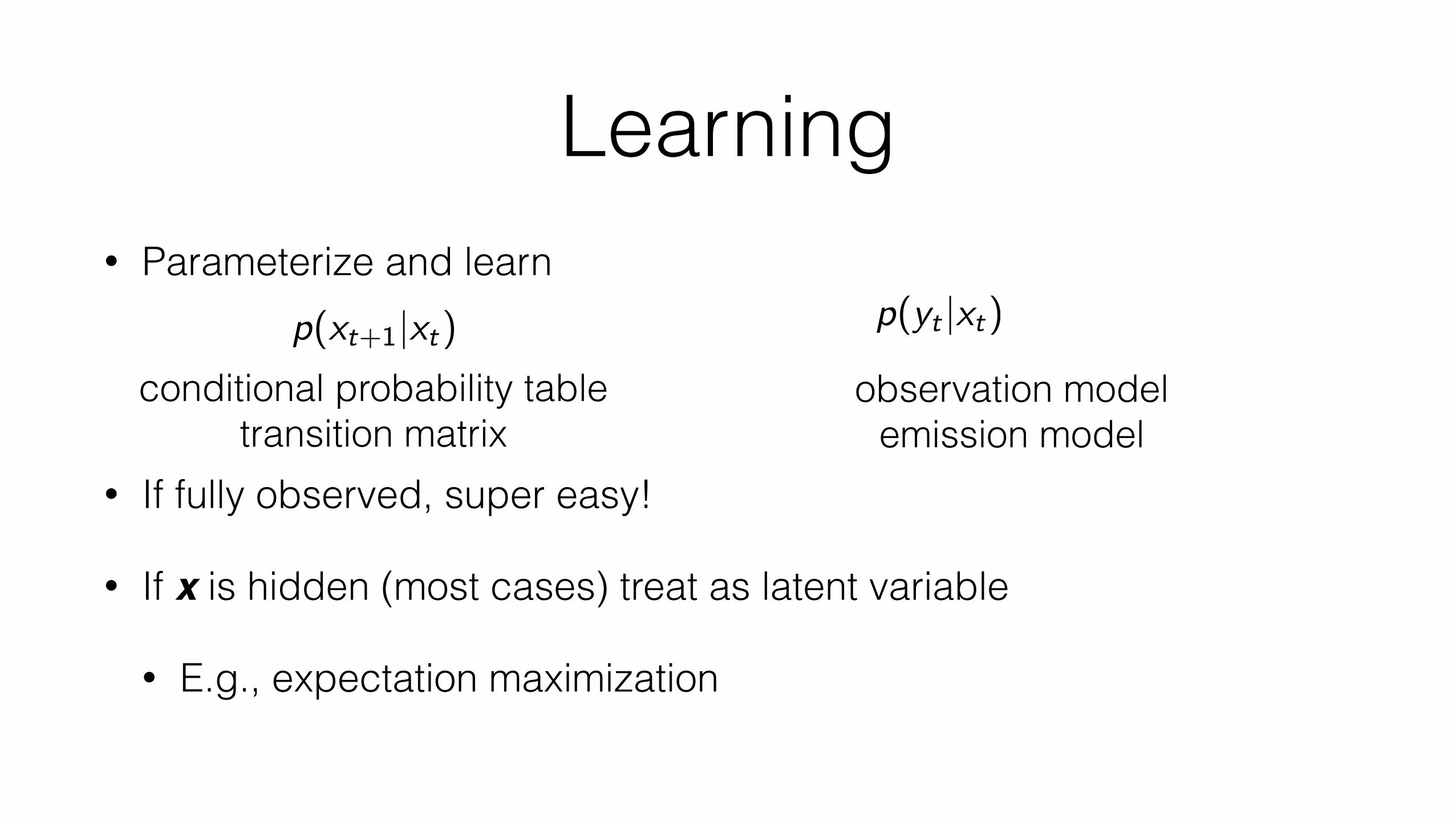
Learning• Parameterize and learn
• If fully observed, super easy!
• If x is hidden (most cases) treat as latent variable
• E.g., expectation maximization
p(xt+1|xt) p(yt |xt)
conditional probability table transition matrix
observation model emission model

Baum-Welch Algorithm
EM using forward-backward inference as E-step
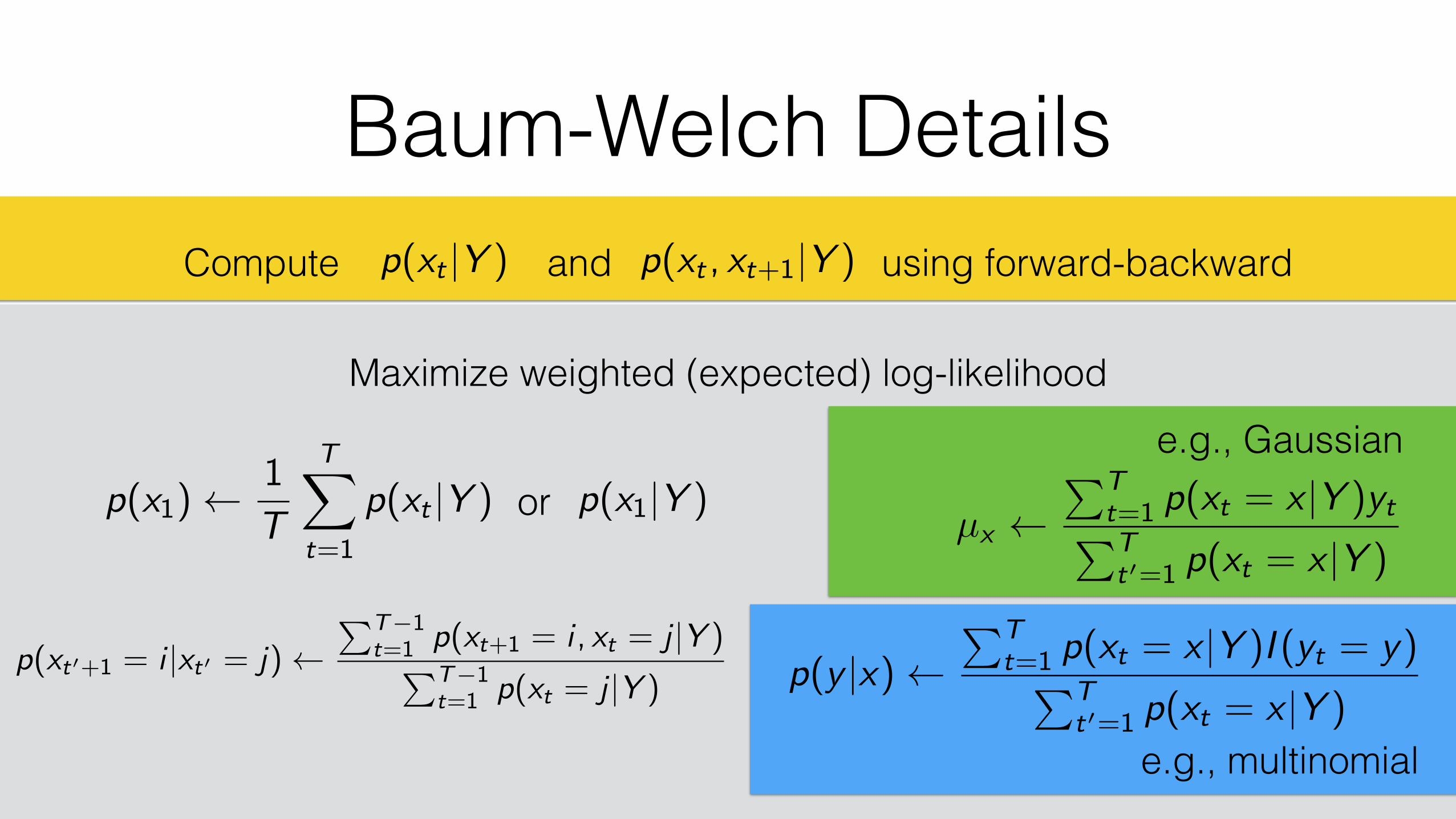
Maximize weighted (expected) log-likelihood
Baum-Welch Detailsp(xt |Y )Compute using forward-backwardp(xt , xt+1|Y )and
p(x1) 1
T
TX
t=1
p(xt |Y ) p(x1|Y )or
p(xt0+1 = i |xt0 = j) PT�1
t=1 p(xt+1 = i , xt = j |Y )PT�1
t=1 p(xt = j |Y ) p(y |x) PT
t=1 p(xt = x |Y )I (yt = y)PT
t0=1 p(xt = x |Y )
e.g., multinomial
e.g., Gaussian
µx
P
T
t=1 p(xt = x |Y )ytP
T
t
0=1 p(xt = x |Y )
Summary• HMMs represent hidden states
• Transitions between adjacent states
• Observation based on states
• Forward-backward inference to incorporate all evidence
• Expectation maximization to train parameters (Baum-Welch)
• Treat states as latent variables


