
Draft – 05/24/2011
Quality Assurance Project PlanQuality Assurance Project Plan for EPA
funded grant PC-00J281-01: WDOE Channel Migration Assessments
Puget Sound SMA StreamsEPA Region 10 Scientific and Technical
Investigation Grant
May 2011Publication No. 11-03-1xx

Publication Information
Each study conducted by the Washington State Department of Ecology (Ecology) must have an approved Quality Assurance Project Plan. The plan describes the objectives of the study and the procedures to be followed to achieve those objectives. After completing the study, Ecology will post the final report of the study to the Internet.
The plan for this study is available on Ecology’s website at www.ecy.wa.gov/biblio/11031??.html
Ecology’s Activity Tracker Code for this study is xx-xxx.
Author and Contact InformationPatricia L Olson, Senior Hydrogeologist, PhD, LHG P.O. Box 47600 Shorelands and Environmental Assistance ProgramWashington State Department of EcologyOlympia, WA 98504-7600
This plan was prepared by a licensed hydrogeologist. A signed and stamped copy of the report is available upon request.
For more information contact: Communications Consultant, phone 360-407-6834.
Washington State Department of Ecology - www.ecy.wa.gov/
o Headquarters, Olympia 360-407-6000
o Northwest Regional Office, Bellevue 425-649-7000
o Southwest Regional Office, Olympia 360-407-6300
o Central Regional Office, Yakima 509-575-2490
o Eastern Regional Office, Spokane 509-329-3400
Any use of product or firm names in this publication is for descriptive purposes only and does not imply endorsement by the author or the Department of Ecology.
If you need this document in a format for the visually impaired, call 360-407-6834.
Persons with hearing loss can call 711 for Washington Relay Service.
Page 0

Persons with a speech disability can call 877- 833-6341.
Page 1

Quality Assurance Project Plan for EPA funded grant PC-00J281-01: WDOE Channel Migration
Assessments
Puget Sound Region SMA StreamsEPA Region 10 Scientific and Technical Assistance
GrantsMay 2011
Approved by:
Signature: Date:
Burney Hill, EPA, Project Officer, EPA Region 10
Signature: Date: name, EPA, QA Manager, EPA Region 10
Signature: Date: Patricia L Olson, Author / Project Manager & Principal Investigator, SEA
Signature: Date: Brian Lynn, Author’s Unit Supervisor, SEA
Signature: Date: Gordon White, Author’s Program Manager, SEA
Signature: Date: Bill Kammin, Ecology Quality Assurance Officer
Signature: Date:
Signatures are not available on the Internet version.
SEA: Shoreline and Environmental Assessment Program
Page 2

Table of Contents
Page
List of Figures and Tables........................................................................................................................4
Abstract........................................................................................................................................................... 5
Project Description and Objectives.....................................................................................................5
Background............................................................................................................................................ 5
Description............................................................................................................................................. 6
Project Purpose.................................................................................................................................... 7
Project Objectives................................................................................................................................ 8
Organization and Schedule..................................................................................................................... 8
Project personnel organization/responsibilities..................................................................8
Project schedule.................................................................................................................................11
Secondary Data..........................................................................................................................................12
Secondary data sources/specification.....................................................................................12
Quality Control Procedures..................................................................................................................16
Secondary data requirements.....................................................................................................16
Procedures for quality control of the secondary data and derived products........17
EPA evaluation of quality of data...............................................................................................18
Data analysis, interpretation, and management.........................................................................18
Data analysis methods....................................................................................................................18
Assessment Method: Existing channel migration studies...............................................20
Field verification................................................................................................................................21
Data reduction....................................................................................................................................22
Statistical analysis.............................................................................................................................23
Reporting..................................................................................................................................................... 25
Deliverables.........................................................................................................................................25
GIS Derived Products.......................................................................................................................25
Final Reports.......................................................................................................................................26
References................................................................................................................................................... 27
Appendices.................................................................................................................................................. 29
Appendix A. Draft Data Management Memo........................................................................30
Page 3

DRAFT - Technical Memorandum.............................................................................................31
Ecology CMZ Project Data Management Outline:...............................................................31
Appendix B. Relative water surface elevation methods.................................................35
Method 1: Relative Surface Model: Tin Interpolation (GeoEngineers).....................36
Method 2: Relative Water Surface Elevation (RWSE).......................................................39
TIN Interpolation Methodology..................................................................................................39
Method 3: Relative Water Surface Elevation (RWSE).......................................................47
IDW Interpolation Methodology................................................................................................47
Appendix C. Data Reduction Forms.........................................................................................54
Form 1: Summarized information for general mapping description and / or maps, photos.....................................................................................................................................................55
Appendix D. Glossary, Acronyms, and Abbreviations......................................................58
Page 4

List of Figures and Tables
Page
Figures
Figure 1: Location of stream reaches to have channel migration zones generally mapped for this project..............................................................................................................................................................7
Figure 2: Organizational chart showing project personnel, major responsibility including QA, and relationship to other project participants.............................................................................................................................................................9
Tables
Table 1: Qualifications and responsibilities for key staff are listed below..............................................................................................................................................................9
Table 2: Proposed schedule for completing project tasks and reports and lead staff.............................................................................................................................................................11
Table 3: The data, source and use of GIS data in this project is listed. .............................................................................................................................................................13
Table 4: Matrix showing the assumed dominant processes, variability, biodiversity by valley geology setting.............................................................................................................................................................24
Page 5

AbstractRiver floodplains and channel migration zones (CMZs) are ecologically productive areas heavily impacted by development. Their importance is detailed in the NMFS Biological Opinion declaring the FEMA program results in “take” of Puget Sound Chinook salmon and steelhead. Flood hazards consist of both inundation and erosion (channel migration). Understanding the extent of a CMZ is critical to assessing risks to development as well as habitat. The Shoreline Master Program (SMP) requires identifying CMZs but this has not been done for over 550 miles of Puget Sound shorelines. Moreover, already completed CMZs methods and delineations are not consistent and often do not address future erosion risks and the loss of historic CMZ areas due to development. Current methodologies do not include evaluating future channel response to altered hydrologic and sediment regimes from climate change and development. Tasks include updating the CMZ mapping methodology, map areas for baseline trend analysis, and develop technical assistance for integrating with SMP and floodplain management and restoration/protection strategies including climate change scenarios.
Project Description and Objectives BackgroundThe project is funded through the U.S. Environmental Protection Agency, Region 10 Puget Sound Scientific Studies and Technical Investigations Assistance Program in Support of Implementing the Puget Sound Action Agenda. The Puget Sound Partnership (PSP) has identified loss of floodplain functions and processes as a threat to ecosystem benefits in six of their eight project areas. The PSP action strategies include reconnecting floodplains, side channels and increasing channel complexity and implementing the state Shoreline Master Program (SMP) and Floodplain Management Programs. Priority Action A.2 identifies permanently protecting the intact areas of the Puget Sound ecosystem that still function well as a keystone piece of Puget Sound protection. The Action Agenda Priority A also addresses identifying areas at immediate risk to conversion or development and updating Shoreline Master Programs as near-term actions.
In the Puget Sound ecoregion, channel migration is the primary floodplain geomorphic process that creates a shifting mosaic of habitat patches of different ages within the river corridor (Fetherston et al 1995). This mosaic provides highly productive ecological areas for aquatic organisms as well as terrestrial species. The channel migration processes occur on a variety of spatial and temporal scales from local bank erosion to avulsions that create many kilometers of new channel to entire reworking of floodplains. Rivers erode some patches each year while other patches accrete sediment and gradually rise in elevation above the river bed (Nanson and Beach, 1977; Brummer, Abbe and others 2006). The high density of complex boundaries between ecotones (Ward et al 1999) creates more environmental complexity, maintained by interactions between river channels and floodplain forests.
The regulatory and legal environment also recognizes the importance of channel migration processes and areas in creating critical habitat in the Puget Sound. In accordance with the judicial order in NWF v. FEMA, 345 F. Supp. 2d 1151 (W.D. Wash. 2004), the National
Page 6

Marine Fisheries Service (NMFS) Biological Opinion declared the Federal Emergency Management Agency (FEMA) floodplain management program results in a “take” of Puget Sound Chinook salmon, steelhead and Orca whales (NMFS 2008). The NMFS opinion allows for reasonable and prudent alternatives to be implemented that would avoid the likelihood of jeopardizing the continued existence of listed species or result in destruction or adverse modification of critical habitat. The NMFS discussed with the FEMA the availability of a reasonable and prudent alternative that the FEMA can take to avoid violation of the Endangered Species Act section 7(a)(2) responsibilities (50 CFR 402.14(g)(5)). The FEMA lists the Washington State Shoreline Master Program updates as a reasonable and prudent alternative to implementing the channel migration requirements of the biological opinion.
The Washington State Shoreline Master Program guidelines, administered through the Washington Department of Ecology, identify channel migration areas as critical freshwater habitats. The SMP guidelines require general identification of CMZs [WAC 173-26-201(3)(c)(vii):] and restrict type and extent of development in these areas in order to protect critical habitat and reduce hazards to public and infrastructure. Yet the quality of mapping efforts to date has been inconsistent and not done for most of the Puget Sound.
In contrast, channel migration is also a flood hazard to people, property, critical infrastructure, and potential pollutant sources such as waste water treatment sites and old landfills that are located within floodplains. Where rapid migration occurs, risk to people and infrastructure often is much greater than flooding alone. This contrast creates an inherent conflict between land uses and the beneficial services provided by floodplain ecosystems. Control of channel migration processes including channelization, dredging, gravel mining, levees, dikes, bank hardening and wood removal has contributed to listing of salmon under the Endangered Species Act (NMFS 2008).
These stressors have consequences not only for the sustainability of fluvial ecosystems but also society. The extent of flood inundation is becoming a greater societal issue as floodplain natural functions such as storage and aquatic habitats are lost due to increased floodplain development. The sustainability of these ecosystems is important for traditional cultures and present and future regional economics.
DescriptionIn August 2009, Ecology identified approximately 550 miles of shoreline stream in the Puget Sound Basin having channel migration potential using geology and soil erosion potential, valley to channel characteristics, orthophoto time series, and LiDAR (Figure 1). The purpose was to provide information to communities updating their Shoreline Master Programs. However, this information only identified potential and not the spatial channel migration area, processes, habitat, floodplain condition or hazards. This study will build on this analysis.
Existing channel migration assessments will be compiled and evaluated in terms of usefulness for identifying hazards and protection and restoration opportunities. This information will be discussed under an update of best available science literature and information on processes and delineation methodologies. Methods described in Rapp and Abbe (2003) and in the Ecology’s channel migration web guidance (Olson 2008) will be used and results will be compared. Using information synthesized from literature review
Page 7

and the method comparisons, we will identify and map channel migration areas and habitats, areas for protection and restoration, high hazard areas, and evaluate relationships between valley setting, migration, channel planform, habitat and climate change.
Figure 1: Location of stream reaches to have channel migration zones generally mapped for this project.
Archival mapping methods have been the mainstay of channel migration analyses and mapping for over 2 decades (e.g., Collins et al 2003, Rapp and Abbe 2003). Mapping the historic and current channel migration area is not by itself adequate to address hazards and restoration questions. For example, air photos and archival maps have limitations for evaluating channel migration on smaller streams that are heavily vegetated. Other methods such as LiDAR, stream power analyses (e.g., Church 2002), geology and soils, valley configuration, and field observations will be used and evaluated for streams where traditional archival mapping does not work. Key elements for delineating a CMZ, as discussed in Rapp and Abbe (2003), but which have not been applied in much of the CMZ mapping to date involve the erosion potential of earth materials, the influence of vegetation (e.g. Michelli et al. 2004), and geotechnical setbacks along high banks susceptible to erosion. These elements will be included in our assessment.
Project PurposeProvide channel migration maps to the Puget Sound local communities for their SMP updates and floodplain management; evaluate existing channel migration methods and assessments as to
Page 8

their usability for predicting future channel response under different development and climate change scenarios; refine the existing Ecology decision framework for conducting channel migration assessments using appropriate methodologies; and update existing scientific literature review documents.
Project ObjectivesThe project objectives are:
To generally map the channel migration area along approximately 550 stream miles (Figure 1) in the Puget Sound region for inclusion in local community Shoreline Master Program updates (WAC 176-26-201(3)(vii) and floodplain management.
Evaluate existing channel migration assessments and delineations on differences and adequacy in addressing future conditions under increased sediment and peak flow due to development and climate change and reducing hazards to people, infrastructure and critical habitat.
Update the existing Ecology channel migration scientific literature review document (Rapp and Abbe 2003) regarding channel migration and response.
Refine existing channel migration methodologies based on credible science and lessons learned from previous tasks and test methods on a subset of streams.
Evaluate method results in terms of actions such as placement of future development, protection and restoration under existing and climate change scenarios.
Update CMZ guidance documents based on components 1 and 2.
Organization and ScheduleProject personnel organization/responsibilitiesThe Washington Department of Ecology, Shorelands and Environmental Assistance Program is the project lead. Dr. Patricia Olson is the Project Manager and Principal Investigator. Ecology has hired consultants and University of Washington staff to assist on the project. Project organization, titles, relationships among participants and QA responsibilities are outlined in Figure 2, Table 1.
Page 9

WA Dept of EcologyPatricia L Olson, PhD, LHG
Principal InvestigatorProject Manager, Project QA
WA Dept of EcologyJerry Franklin, MS
GIS LeadSEA GIS QA team lead
Cardno EntrixTim Abbe, PhD, LEG, LHG
Principal in charge, Science director
University of Washington, Earth and Space Sciences
Brian Collins, PhD, Research ScientistScience advisor
Cardno EntrixEric Harlow, MS, CFM
Project Manager
Cardno EntrixTim Abbe, PhD, LEG, LHGSenior Technical Director,
Internal QA
Cardno EntrixMike Ericson, MS
Shawn Higgins, MSGeomorphology/hydrology
Cardno EntrixJenna Scholz, MS
Stakeholder facilitation
GeoEngineersMary Ann Reinhart, MS, LG, LEG
Senior Technical Director, internal QA
GeoEngineersChris Bellusci, MS PEData management
Data management/sharing QA
GeoEngineersJodie Lamb, MS LG, LEG
Geomorphology/hydrology
Consultant Science/technical project support
Figure 2: Organizational chart showing project personnel, major responsibility including QA, and relationship to other project participants
Table 1: Qualifications and responsibilities for key staff are listed below.
Name Title Responsibility
Patricia Olson, PhD, LHGphone: 360-407-7540email:[email protected]
Ecology, senior scientist (hydrogeology series) for SEA program with focus on stream hydrology and fluvial geomorphology
Principal Investigator and overall Project Manager. Science and technical lead for project, review methods and products, CMZ mapping and revised methods, science literature review, Writes the QAPP, conducts QA review of data, analyzes and interprets data. Writes the draft report and final report
Jerry Franklin, MSphone: 360-407-7470email: [email protected]
Ecology, SEA program senior GIS staff, floodplain mapping
Project lead GIS staff, develop GIS methods, evaluate GIS data, coordinates with GeoEngineers data management and GIS staff, conducts QA review on GIS data, assists Project manager on writing QAPP
William R. Kammin Phone: 360-407-6964
Ecology Quality Assurance Officer
Reviews the draft QAPP and approves the final QAPP.
Page 10

Brian Collins, PhD Univ. of Wash., Earth and Space Sciences, Research Scientist, Fluvial geomorphology and GIS
Provide CMZ delineation review, review science documents, develop channel migration typology
Tim Abbe, PhD, LEG, LHG Cardno ENTRIX, Technical Director, Vice-President, Geomorphology/restoration program manager
Project scoping and design, senior science and technical review, internal QA
Mary Ann Reinhart, LG, LEG
GeoEngineers Associate Fluvial Geomorphologist & Geologist
Technical lead for GeoEngineers, senior analyst and reviewer, internal QA
Eric Harlow, MS, CFM Cardno ENTRIX Project Scientist, Hydrologist
Consultant project manager responsible for managing communications and budgets, technical analyst for hydrology and cumulative effects.
Mike Ericsson, MS Cardno ENTRIX Project Geomorphologist
Project geomorphologist, technical analyst for geomorphology, and CMZ delineation
Shawn Higgins, MS Cardno ENTRIX Sr. Staff Geomorphologist
Project geomorphologist, technical analyst for geomorphology and CMZ delineation
Chris Bellusci, PE GeoEngineers Technical Program Manager
GIS lead and database management.
Jodie Lamb, LG, LEG GeoEngineers Sr. Project Geologist
Project geomorphologist, technical analyst for geomorphology and CMZ delineation.
Ecology contracted with Brian Collins, University of Washington through an interagency agreement. Ecology issued an RFP for consultant scientific and technical support. The RFP meet the state requirements for large personal services contracts as well as Federal requirements. Ecology contracted with Cardno ENTRIX as the prime consultant. GeoEngineers is the sub-consultant to Cardno ENTRIX for this project. Cardno ENTRIX and GeoEngineers have committed to working together and with Ecology by signing a teaming agreement that describes how the companies will interact with each other and with Ecology as equal partners. This teaming agreement includes elements that go beyond typical subcontracting agreements. Key elements relevant to this QAPP are:
As teaming partners, both parties are expected to contribute roughly 50 percent of the work effort for both the proposal and the project work scope.
As teaming partners, both parties will be included in, and/or informed of, all communications with Ecology.
Both parties will be fully represented in all work products, including maps, memos, reports, and digital files.
No work products will be submitted to Ecology unless they are reviewed and approved by both Cardno ENTRIX and GeoEngineers.
GeoEngineers will provide data management services for the project team. The data management will be designed to provide full on-demand access to the data base for designated Cardno ENTRIX and Ecology staff. Protocols specific to data base compilation, utilization, and version control will be developed in concert with Ecology and Cardno ENTRIX GIS technical staff.
Page 11

Upon completion of the project, all digital files, including intermediate and final work products, will be distributed to all parties
Project scheduleTable 2: Proposed schedule for completing project tasks and reports and lead staff
Project Management Due date Lead staff
Issue RFP for personal services & hire, hold scoping, data sharing meeting
12/2010 Patricia Olson/Jerry Franklin
Semi-annual reports to EPA Semi-annual: April, Oct
Patricia Olson
Write QAPP 5/2011 Patricia Olson
Assess existing CMZ delineations Due date Lead staff
Evaluate existing CMZ delineations 09/2012 Patricia Olson, Tim Abbe, Mary Ann Reinhart, Brian Collins
Apply CMZ methodologies Due date Lead staff
Update channel migration literature/report due
07/201212/2012
Patricia Olson
Generally map CMZ for SMP 09/2011 Patricia Olson, Tim Abbe, Mary Ann Reinhart, Brian Collins
Submit data/maps to QA review 10/2011 GIS generated data: Jerry Franklin, Maps, reports, models: Patricia Olson, Tim Abbe, Mary Ann Reinhart, Brian Collins
Meet with communities to discuss results & implement
11/2011 Patricia Olson, Ecology regional shoreline and floodplain managers
Streamline methods, identify/specifically assess/map sample stream reaches
09/2012 Patricia Olson, Tim Abbe, Mary Ann Reinhart, Brian Collins
Submit data/maps to QA review 11/2012 GIS generated data: Jerry Franklin, Maps, reports, models: Patricia Olson, Tim Abbe, Mary Ann Reinhart, Brian Collins
Compare previous delineations to new delineations/report
03/2013 Patricia Olson, Tim Abbe, Mary Ann Reinhart, Brian Collins
Create peer review group for external scientific review and QA/QC
10/2012 Patricia Olson
Draft due to peer reviewer 10/2012 Patricia Olson
Update CMZ guidance documents Due date Lead staff
Update CMZ web based guidance and publish hard copies of guidance
09/2013Patricia Olson
Create peer group to review guidance 03/2013 Patricia Olson
Draft due to peer reviewer 04/2013 Patricia Olson
Final (all reviews done) due to Plain Talk 11/2013 Patricia Olson
Page 12

& publications coordinator
Final guidance due on web 01/2014 Patricia Olson/Cedar Bouta
Public Meetings/Disseminate Information Due Date Lead Staff
Final guidance due on web09/2013 Patricia Olson, Jenna Scholz,
Ecology regional shoreline and floodplain managers
Report on meeting, responses 11/2013 Jenna Scholz
Final report Due date Lead staff
Draft due peer reviewer 10/2013 Patricia Olson
Peer review comments incorporated 12/2013 Patricia Olson
Final (all reviews done) due to plain talk and publications coordinator
12/2013Patricia Olson
Final report due on web 02/2014 Patricia Olson/Cedar Bouta
Final report due to EPA 01/2014 Patricia Olson
Secondary Data Secondary data sources/specification In this project Ecology will not be analyzing discrete environmental data. Ecology (and its consultants) will be interpreting and measuring from existing data for identifying the extent of channel migration and erosion and evaluating channel response and developing methodologies. Field observations will consist of verifying a subset of channel migration boundaries. No discrete sampling is proposed. If this changes, specific measurements are including in the field observations an amendment to this QAPP will be provided to EPA.
The project relies primarily on secondary data including:
GIS (Table 3, layers, sources, scale/resolution and purpose).
Historic maps and aerial photography not currently in a GIS environment.
Geologic reports from the USGS and Washington Department of Natural Resources.
Existing channel migration assessments and delineations.
Photographs, restoration projects and other information that shows channel conditions.
Data generated from other EPA funded projects such as the Puget Sound Watershed Characterization Project and the NetMap project. The later will provide information on sediment sources, delivery and routing to streams.
Page 13

Table 3: The data, source and use of GIS data in this project are listed. State Acronyms: University of Washington (UW); Washington Department of Natural Resources (DNR); Washington Department of Fish and Wildlife (WDFW); Washington Department of Ecology (Ecology); Washington Department of Transportation (WDOT). All have metadata that meets the Washington State Geographic Information Council Geospatial Data Guidelines or FGDC Content Standards for Digital Geospatial Metadata.
Data Source/custodian Scale/ resolution
Purpose
National Hydrography Data USGS/EPA 1:24k Base streamline layer for comparison to stream location in aerial photograph time series assessment
SSURGO soil data NRCS 1:24k Soil erosion potential for floodplains and stream banks (see attachment A for method)
Washington State Geology DNR 1:100k Geology erosion potential and sediment source information. The larger map scale on Geology layers does not alter the final products for channel migration maps because the geology detail is sufficient to identify erosion potential and sediment sources
Liquefaction Susceptibility DNR 100k
Landslides (DGER) DNR-DGER 1:24k
LiDAR Puget Sound LiDAR consortium
2 meter horizontal accuracy; vertical accuracy
Mapping channels and producing relative water surface elevation maps, developing channel and valley characteristics such as gradient, channel width, sinuosity, confinement, stream power
DEM 10 m UW/USGS 24k The 10 meter DEM is used to evaluate general valley and stream characteristics, for example, valley and stream gradient, valley configuration where LiDAR is not available.
DEM 10 meter hillshade Ecology 24k
NAIP orthophotos National Agricultural Imagery Program
Various resolutions
Mapping channel location over time and measuring migration rates over time. The historic channel migration zone boundaries are determined from current and historic stream locations. ESRI imagery data used to evaluate stream conditions and proposed channel migration maps on a 3-D platform (Arc Explorer). Note: Because of certain license
DOQQ USGS 36 inch horizontal accuracy
Page 14

restrictions, Ecology cannot use Google Earth. However, consultants can use it and will use it. The imagery is the same.
Washington State 24K DRG Image Library
USGS 1:24k
ESRI World satellite imagery ESRI NA
Historic air photos, maps Puget Sound River History Project, UW
various
LandSat Images 1972-2010 USGS/Ecology 30-meterProvides information on large changes in land use, wetlands, and stream planform pattern (meander, straight, braided, multi-channel.
Land Cover: 1991-2006 NOAA NA Provides information for evaluating channel response related to changes in land cover that influence sediment and hydrologic regimes and delivery
Impervious surface: 1986-2006
Sanborn/NOAA NA
Forest Canopy 1991-2006 Sanborn NA
FEMA Flood Hazard Zones FEMA 1:24kLocation of FEMA floodplains in relation to channel migration areas and developing channel migration erosion hazard maps
Shoreline Management Act (SMA) Suggested Arcs
Ecology 1:24k Provides location of the upstream point for state shorelines
Priority and critical species and habitat
WDFW NA For identifying reaches with priority and critical habitat
Salmon and Steelhead Habitat Inventory and Assessment Program (SSHIAP)
WDFW 1:24k
For evaluation fish related conditions for identifying important fish habitat reaches
ESA Salmon Listing NOAA-NMFS 1:100k For identifying reaches with ESA salmon species
Salmon Recovery Regions WDFW 1:500kIdentifying reaches salmon recovery needs ,existing Endangered Species Act listings, proposed listings, and where there is a strong likelihood for future listings
Page 15

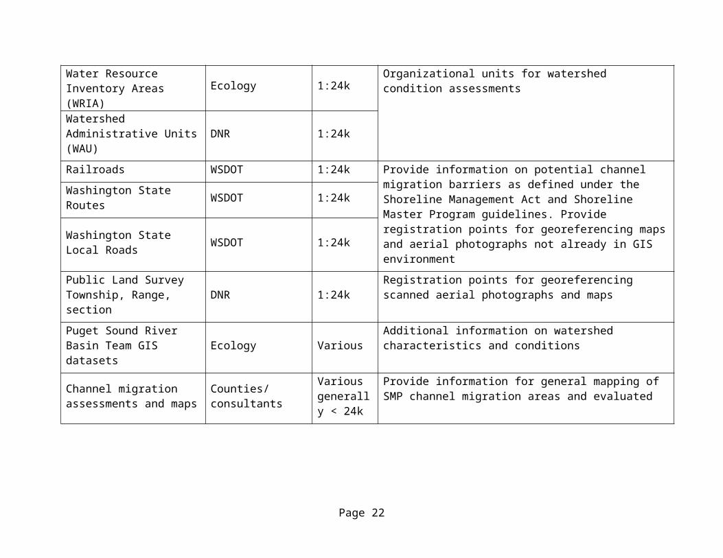
Water Resource Inventory Areas (WRIA)
Ecology 1:24k Organizational units for watershed condition assessments
Watershed Administrative Units (WAU)
DNR 1:24k
Railroads WSDOT 1:24k Provide information on potential channel migration barriers as defined under the Shoreline Management Act and Shoreline Master Program guidelines. Provide registration points for georeferencing maps and aerial photographs not already in GIS environment
Washington State Routes WSDOT 1:24k
Washington State Local Roads
WSDOT 1:24k
Public Land Survey Township, Range, section
DNR 1:24kRegistration points for georeferencing scanned aerial photographs and maps
Puget Sound River Basin Team GIS datasets
Ecology VariousAdditional information on watershed characteristics and conditions
Channel migration assessments and maps
Counties/ consultants
Various generally < 24k
Provide information for general mapping of SMP channel migration areas and evaluated
Page 16

Quality Control Procedures Secondary data requirements The Washington Department of Ecology (Ecology) has no agency QAPP for using secondary data nor does it have quality metrics for assessing channel migration or channel response processes. Quality metrics or standard operating procedures are generally available through Ecology’s GIS/IT program. These, in addition to project specific requirements, are used to develop quality requirements and quality control.
All GIS data will meet the Washington State Geographic Information Council Geospatial Data Guidelines or FGDC Content Standards for Digital Geospatial Metadata and National Map Accuracy Standards.
Ecology uses the following data storage and import standards. All GIS data, if not in the datum, projection and coordinate system listed below will be projected into these. All GIS data produced for this project will meet these standards.
Horizontal Datum NAD 83 HARN*
Vertical Datum NAVD-88**
Projection System Lambert Conic Conformal
Coordinate System Washington State Plane Coordinates
Coordinate Zone South (or zone-appropriate if not statewide)
Coordinate Units U.S. Survey Feet
Accuracy Standard +/-40 feet or better
Vector Import Format ArcExport E00 file, Shapefile, File Geodatabase, Personal Geodatabase
Raster Import Format TIFF, BIL/BIP, RLC,GRID, ERDAS
MetadataFederal Geographic Data Committee (FGDC), Metadata Content Standards*
* More information is available on the Washington Geographic Information Council (WAGIC) website at http://wagic.wa.gov/Techstds2/standards_index.htm.
** North American Vertical Datum 1988 (NAVD88) as defined by the National Geodetic Survey (NGS) is the official civilian datum for surveying and mapping in the United States.1 The Washington Department of Ecology is adopting NAVD88 as the agency standard vertical datum. All elevation data created by or submitted to Ecology should be collected in or converted to NAVD88. The collection method used to determine elevation should be specified. Elevations may be recorded in either feet or meters as long as the unit of measure is explicitly stated in the metadata
All maps and aerial photographs not in a GIS environment will meet National Map Accuracy Standards.
Standards for Spatial Point Attributes Stored in Non-Spatial Databases (web site): Ecology databases should support the following spatial features and address methods throughout agency level database systems. This structure will insure: consistency; understanding; and ease of integration between both tabular and geospatial data systems. A spatial address refers to the geographic point location of an object, and is used to define the point of that object or "Ecology thing" that information is being collected about (e.g. well, spill, facility). The standard of point data collection method is in latitude-longitude degrees, minutes, seconds. This
Page 17

allows one standard way to collect and report information within the agency. This suggested format will provide the agency with greater pay back in uniformity, ease of data comparison and compilation, and lessen the storage of redundant data.
Published data will have been scientifically peer-reviewed.
Existing channel migration assessments and mapping should meet Ecology standards for GIS data and spatial attributes.
Procedures for quality control of the secondary data and derived products Much of the project GIS data is developed and maintained by county, state and federal agencies (Table xx) and comply with the Washington State Geographic Information Council Geospatial Data Guidelines or FGDC Content Standards for Digital Geospatial Metadata and National Map Accuracy Standards (Geospatial data and map: http://nationalmap.gov/gio/standards/). The accuracy of this information is the responsibility of the agencies and organizations that disseminate the data. Use of such digital databases, in the absence of independent validation of their accuracy, is commonplace in academia, government (including in the EPA), and the private sector.
Ecology has access to these databases and their metadata. This data is shared with Ecology’s consultants for this project. The following outlines our steps for maintaining consistency in GIS analysis, interpretation and management.
All GIS data not in Ecology specified datum, projection and coordinate system listed below will be projected into these. All GIS data produced for this project will meet Ecology standards (http://www.ecy.wa.gov/services/gis/data/standards/standards.htm and http://wagic.wa.gov/Techstds2/standards_index.htm ).
All created data not in GIS will meet Ecology Standards for Spatial Point Attributes Stored in Non-Spatial Databases.
The scale of most of the primary GIS data used in the project scale is 1:24000. This scale is adequate to identify development, erosion potential, base streamline, channel planform pattern (meander, straight, multi-channel, and braided), valley characteristics and form, riparian vegetation change, and other factors that influence channel migration processes. Products produced from this data will adhere as closely as possible to National Map Accuracy Standards for 1:24000 scale maps. The standard specifies that 90 percent of well-defined features are to be within 0.02 inches, which is 40 feet, of the true mapped ground position. Some existing geospatial data that is to be incorporated into the GIS is originally produced at scales smaller than 1:24000. The positional accuracy of the data will be refined by editing point and vertice positions to match the features as they appear on an aerial image that meets the required accuracy.
All GIS products developed in this project will be reviewed by the GIS Lead (Jerry Franklin) and Chris Bellusci (GIS Lead, GeoEngineers) for accuracy and meeting GIS standards and to insure that data processing uses consistent GIS methods and that data interpretation follows a consistent sequence. Review will include evaluating consistency, map accuracy, and data limitation assumptions and appropriateness.
Page 18

Data will be managed by Chris Bellusci as per draft memo, May 18, 2011 (Appendix A).
All products developed in this project will go through a quality review by the Project Manager (Patricia Olson) and consultant technical and scientific leads (Tim Abbe, Mary Ann Reinhart). The review includes checks for computational accuracy, technical soundness of analysis, reasonableness of results and conclusions, clarity of presentation, and appropriateness of the limitations of the data. All reviewers are licensed geology professionals in Washington and must adhere to highest standards as per licensure requirements.
Historic maps and aerial photographs created by the federal agencies usually meet the National Map Accuracy Standards. Published maps meeting these accuracy requirements shall note this fact in their legends, as follows: "This map complies with National Map Accuracy Standards." Published maps whose errors exceed those standards must omit from their legends all mention of standard accuracy. In those cases, the accuracy of any map may be tested by comparing the positions of points whose locations or elevations are shown upon it with corresponding positions as determined by surveys of a higher accuracy.
Existing channel migration assessments and maps will be reviewed based on Ecology GIS and spatial attribute standards and products will be tested for accuracy by comparing positions of known features from GIS data with higher standards or accuracy.
EPA evaluation of quality of data
EPA will not be evaluating the quality of the secondary data. A disclaimer will be added to any project deliverable to indicate that the quality of the secondary data has not been evaluated by EPA for this specific application.
Example Disclaimer Language: The Environmental Protection Agency is not responsible for insuring that the secondary data and subsequent products meet specified data quality and accuracy standards. Washington Department of Ecology is the responsible agency for insuring data quality and accuracy for this project.
Data analysis, interpretation, and management Data analysis methodsArchival mapping methods have been the mainstay of channel migration analyses and mapping for over 2 decades (e.g., Collins et al 2003, Rapp and Abbe 2003). Channel migration change over time is generally identified from historic maps and orthophotos and field verification and measurements. In this project mapping of channel migration stream lines, active channel, channel bars and other fluvial landforms, channel width and gradient, valley width and gradient over time is done at a display scale of 1:5000 or less. Most GIS aerial photographs and orthophotos (Table 3) resolutions are sufficient for mapping at this display scale.
Page 19

While channel migration assessment methods based on secondary data are well developed and reported in peer-reviewed science literature these methods may not apply for some conditions:
Erosion potential or erosion hazard area: Lahar, glacial or fluvial terraces can be easily eroded by channel migration processes. Vegetation (e.g. Michelli et al. 2004) also influences bank and floodplain susceptibility to erosion. Most channel migration assessments do not include geotechnical setbacks along high banks susceptible to erosion or the influence of vegetation. These erosion processes and controls are not always obvious from the aerial photograph and map record. Methods to identify and quantifying these processes without more extensive field evaluation will be evaluated. Methods include using regime theory models (e.g. Millar 2000, 2005) and bank stability models (e.g. Simon, A., Langendoen 2006).
Small streams with vegetation canopy: air photos and archival maps have limitations for evaluating channel migration on smaller streams that are heavily vegetated. Other methods such as LiDAR, stream power analyses (e.g., Church 2002), geology and soils, valley configuration, and field verification will be used.
Recent channel response to development and climate change: The relationships are not well documented in historic maps, aerial photographs or other secondary data sources. New USGS and National Park studies identify some streams that are responding to changes in headwaters glaciers and provide channel dimension and sediment data and other relevant information documenting recent changes. The channel and sediment data from these studies can be used to identify the magnitude of change and possible trajectories for future channel response. Increase in peak flows can also alter channel response. Peak flow hydrograph analysis using Bulletin 17B procedures incorporated into the USGS model PEAKFQ (Flynn et al 2006a, 2006b). The peak flow analysis is done on the entire annual peak flow record, and then the time series are divided into pre-change and post-change series. Records before Water Year (WY) 1950 are often used for the pre-climate change series. On gages without long-term records, the time series comparison is 1) earliest record to most recent annual peak flow; 2) 1970 to present.
Part of this project is to develop new methods where standard methods do not apply. Analysis methods are being developed to meet the 3 conditions listed above. Remote sensing will continue to play a critical role in our analysis because it is the most practical and cost-effective way, to evaluate and understand time-sensitive processes important to creating fluvial responses and landforms especially in terms of varying temporal and spatial scales. In particular, LiDAR (LIght Distance And Ranging, also known as Airborne Laser Swath Mapping or ALSM), in combination with digital high resolution orthophotos and aerial photographs, will be used to develop higher resolution DEMS to identify and measure landforms and to some extent human created features in the floodplain, determine vegetation canopy coverage; habitat type, channel migration history, quantify changes in the geomorphic floodplain; and assess flood and erosion hazards such as avulsions.
Relative water surface elevation models, also called height above water surface (e.g. Jones 2006) created from the LiDAR bare earth DEMS provide information on channel location
Page 20

and features, fluvial and hillslope processes over time and potential avulsion paths. Methods are included in Appendix B. The results of the 3 relative water surface elevation methods will be compared across valley configuration and stream pattern to determine if all methods: 1) provide equivalent results, 2) one provides better results across all valley configurations; or 3) different methods provide better results based on valley configuration or channel planform pattern.
LiDAR will be used to evaluate results of channel migration assessment methods that used standard archival methods without using LiDAR. LiDAR will be used also to evaluate more practical and cost-effective tools for local communities to identify channel migration areas for floodplain and shoreline management, areas for ecological protection and/or restoration and identify relevant processes and templates for restoration. LiDAR bar earth data area also used to measure channel width and gradient for stream power analyses as well as develop relative water surface elevation models and identify historic and current fluvial landforms in the valley bottoms.
The channel gradient data is used for a stream power analysis. Unit stream power indicator (fluid density ( ), acceleration of gravity (g)*channel gradient (S)* effective discharge ρ(Q) /active or bankfull channel width (w)) provides information on stream sediment transport capacity that is the ability of the stream to transport sediment:
P= ρgSQw
Stream power from this equation is watts per unit channel width or unit power (Newton·m s-1). High transport capacity can result in channel incision and bank erosion. Low transport capacity may cause channel aggradation. Bankfull discharge can be calculated from instantaneous annual peak flow data available from USGS or Ecology stream gages. On streams that have no discharge gage stations or none in close proximity to reaches of interest, the USGS Streamstats program will be used to estimate the bankfull flood discharge (http://water.usgs.gov/osw/streamstats/Washington.html). Our definition for bankfull discharge is the discharge where sediment transport, channel movement and other geomorphic work is done.
Although the average bankfull discharge in Washington approximates the 1.4-1.5-year flood frequency (Castro and Jackson 2002), the bankfull discharge varies depending on channel geometry and other factors. Since there are no predictive equations for these flood recurrence intervals, we assume that the 2-year flood is bankfull.
GIS analysis, interpretation and mapping of vegetation, floodplain landforms, channel migration and floodplain inundation boundaries will be done in ArcGIS 9.xx and 101. Office delineation will be followed up with field inspections to refine delineation and assess the accuracy of remote sensing and GIS methods.
Assessment Method: Existing channel migration studiesKey questions include:
1) Were the CMZs constrained by infrastructure?
2) How were rates of migration determined?1 Ecology has not updated to ArcGIS 10 yet. But our consultants use ArcGIS 10.
Page 21

3) System classification system: (based on typology being developed in this project?
4) How were soil types considered?
5) Was LiDAR used?
6) What protocol was used?
7) Classification date relative to storm events and determination of key storm events since?
8) How much field data was collected? (Desktop vs. field classification)
9) Were changes in hydrology or climate change considered?
10) Were changes in sediment supply or transport capacity considered?
11) Was the influence of riparian vegetation considered?
12) Were avulsions considered? If so, how were they considered?
Once the evaluation criteria have been established and significant events in each basin identified, an evaluation matrix will be populated by applying the evaluation criteria to the existing CMZ delineations.
The individual CMZ delineations will be evaluated to see how it responded to recent storm events by comparing delineations and stream banks with recent aerial photos or LiDAR maps. Areas with poor coverage or obscured by riparian cover will be identified. Past CMZ delineations will be classified as having passed, where the current channel configuration is within that predicted by the report, or failed, where the streams exceeded mapped CMZ delineations or moved at a rate faster than predicted. Passing streams will be further subdivided into the following categories: a) no significant events occurred within the basin, b) a significant event occurred and the method and margin of safety was appropriate, and c) a significant event occurred, but the method or the margins of safety were inappropriate. A report will be prepared focusing on the streams that failed, the streams that passed for the wrong reasons, and an analysis of the probable causes. Project staff will not evaluate reports authored by their own company.
Field verificationField verification of fluvial features and channel migration processes and boundaries will be done on some stream reaches. For the SMP general CMZ maps, field verification will be done on a as needed basis. Need is defined as the reaches, mostly smaller streams with heavy canopy cover, where channel migration processes could not be determined remotely. For evaluating previously existing channel migration assessments and new methodologies, sample reaches will be chosen using a stratified approach where valley geologic setting is the top-level stratification, the next level is landscape units (e.g., alluvial fan, fluvial valley, hillslope-stream valley), and then channel planform.
The locations of fluvial features related to channel migration and identifiable channel migration indicators and boundaries and other significant features will be recorded using an automated GPS/GIS field mapping system. GIS base map data will be transferred to the mobile GPS/GIS mapping system (Trimble Geo XT, sub meter, with GPS Pathfinder Office and TerraSync Professional field software). The location of known targets for mapping will be entered or marked in the system. The GPS/GIS mapping system will be used to navigate
Page 22
to GIS mapped boundaries and fluvial features. Ecology has standard operating procedures (SOP) for using hand-held GPS receivers (Janisch, 2006, ECY_EAP_SOP_013AssigningGPSCoordinates, approved 09/6/2006 by Ecology QA Officer). This SOP will be used to maintain QA/QC on GPS measurements. Photographs will be taken with a digital camera and the photo id numbers will be recorded in the GPS/GIS system. All information will be transferred back to the GIS data and attributes added.
Riparian vegetation plays an important role in mediating channel response and channel migration, degree of site disturbance and habitat quality. Riparian vegetation structure will be visually characterized using Ecology SOP for Visual Characterization of Riparian Vegetation Structure for the Extensive Riparian Status and Trends Monitoring Program (Werner, 2009, SOP067VisualCharacterizationofRiparianVegetion_v1_0, approved by Ecology QA Officer, 11/27/2009). This SOP will be used to maintain QA/QC on visual riparian characterization.
Data reductionData reduction forms have been developed for this project (Appendix C). The forms are to:
1. Organize and reduce GIS data and results for general channel migration mapping under Shoreline Master Program guidelines.
2. Reduce data from more detailed assessments including field data.
Each person developing specific data related to this project will use the appropriate forms2. Their data will be independently validated for data emissions or errors by other project staff. Data that is missing is identified and data sources (e.g., GIS, maps, aerial photos etc) are checked to identify data absence reasons. If omission rather than data not available, the data will be added.
Accuracy refers to the closeness of a measured or computed value to its true value, where the true value is obtained with perfect information. Due to the natural heterogeneity and random variability of many environmental systems, this true value exists as a distribution rather than a discrete value. In geomorphic process studies, the underlying distributions for channel response and channel migration are often not known.
Data accuracy or errors instead will be based on the assumption that data generated for a specific parameter falls within an acceptable range of values for that parameter. Data that fall outside of acceptable limits, for example physical constraints on parameters such as channel gradient, channel width, channel location, stream power, and LiDAR generated DEMS and relative water surface elevation models, are identified by staff. These data errors or accuracy will be reviewed and validated by lead or senior project staff: Patricia Olson, Jerry Franklin, Brian Collins, Tim Abbe, and Mary Ann Reinhart.
Statistical analysisGeomorphic data:
The project is exploratory because there is little or no published (or other sources) studies or methods to determine error and bias in cases such as:
2 The data forms may be changed during the project if the current ones do not meet the project data requirements.
Page 23

Conducting channel migration assessments on small streams that are not readily visible on aerial photographs and only coarsely mapped on historic maps.
Channel migration approaches or methodologies addressing migration processes and channel responses by valley configuration, channel planform pattern, land development/management, or changes in sediment or hydrologic reaches.
Quantifying channel migration related erosion hazard areas for lahars, fluvial or glacio-fluvial terraces.
Descriptive statistics such as means, variances, coefficient of variation, minimum and maximum values can be used to provide summary information on variables such as high and peak flows, channel migration rates, changes in active channel parameters, changes in vegetation cover, channel bars, sinuosity and others. Descriptive statistics may also provide measures for testing differences in some parameters, such as migration rates, channel bar changes, stream power between different valley configurations (geologic control) or stream planform pattern for cases where the rate parameters are developed over similar aerial photo and map time series3. Many geomorphic parameters are not normally distributed. Some, such as channel length, can be normalized through a log normal transformation. Other transformations may be needed for other parameters. Non parametric significance tests will be used for those that cannot be normalized.
Detailed inferential and more robust statistical testing methods will not be determined until the project moves into assessing existing channel migration studies and developing channel migration typology. Even then more robust statistical testing may not be particularly useful.
There are limitations to using statistics in this type of study:
Sample size is often very small, e.g., 3-7 aerial photo or map time series.
As is often the case with geomorphic process related investigations, hypothetical testing may not provide a better understanding of real processes involved with channel response and migration in relatively newly disturbed landscapes (e.g. Pleistocene and alp line glaciation, Holocene landslides, earthquakes and other tectonic forces) as well as those being influenced by external factors such as changes in land use or sediment and hydrologic regimes.
o For example, for some streams there is a relationship between peak flow recurrence intervals and channel migration rates or channel response. But in other similar streams, there is no relationship. To make it more challenging, the underlying distributions are not known.
Since geomorphic processes and landscape (channel) responses are highly influenced by interactions between time and space. Multivariate statistics would likely be more useful for evaluating the conceptual or system modeling. Relationships within and among subsystems are depicted with canonical structures usually as a schematic diagram as a geomorphic interpretation of a system model. These diagrams may show
3 Annual migration rates often decrease as time between aerial photographs or maps increases. For example, on the White River, near Buckley, the mean annual migration rate between the 1936 and-2009 photos is 0.75 meters. The mean annual migration rate between 1998 and 2006 is 3.4 meters. The mean annual migration rate between 2006 and 2009 is 6.8 meters.
Page 24
the nature (direct or inverse), direction (dependent/independent), and strength of linkages within and among subsets of variables.
While there are several conceptual models concerning channel response and migration, the underlying theory is not adequately developed particularly for channels in recently disturbed landscapes. The theories become more tenuous where these streams are also responding to changing external factors such as sediment and flood regimes and land development patterns. This also limits the usefulness of standard statistical procedures.
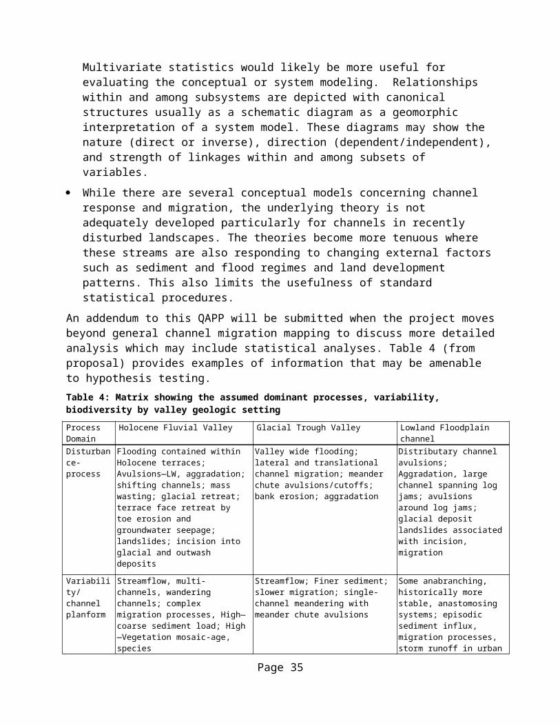
An addendum to this QAPP will be submitted when the project moves beyond general channel migration mapping to discuss more detailed analysis which may include statistical analyses. Table 4 (from proposal) provides examples of information that may be amenable to hypothesis testing.
Table 4: Matrix showing the assumed dominant processes, variability, biodiversity by valley geologic setting
Process Domain
Holocene Fluvial Valley Glacial Trough Valley Lowland Floodplain channel
Disturbance-process
Flooding contained within Holocene terraces; Avulsions—LW, aggradation; shifting channels; mass wasting; glacial retreat; terrace face retreat by toe erosion and groundwater seepage; landslides; incision into glacial and outwash deposits
Valley wide flooding; lateral and translational channel migration; meander chute avulsions/cutoffs; bank erosion; aggradation
Distributary channel avulsions; Aggradation, large channel spanning log jams; avulsions around log jams; glacial deposit landslides associated with incision, migration
Variability/ channel planform
Streamflow, multi-channels, wandering channels; complex migration processes, High—coarse sediment load; High—Vegetation mosaic-age, species
Streamflow; Finer sediment; slower migration; single-channel meandering with meander chute avulsions
Some anabranching, historically more stable, anastomosing systems; episodic sediment influx, migration processes, storm runoff in urban areas
Biodiversity Highest Medium-high High
Hydrologic peak flow data:
Hydrologic characteristics are more amenable to statistical analysis and transformations to meet statistical test assumptions (e.g. normally distributed). Bulletin 17B (Interagency Advisory Committee on Water Data, 1982) will be used to evaluate and summarize instantaneous annual peak flow for changes over time. Bulletin 17B is the standard used by Federal agencies such as USGS, FEMA and USCOE for determining flood recurrence intervals. The USGS software PeakFQ is used to calculate recurrence intervals and annual exceedance probabilities based on Bulletin 17B (Flynn et al 2006a, 2006b). PeakFQ provides estimates of instantaneous annual-maximum peak flows for a range of annual-exceedance probabilities of 0.6667, 0.50, 0.4292 0.20, 0.10, 0.04, 0.02, 0.01, 0.005, and 0.002. The Pearson Type III frequency distribution is fit to the logarithms of instantaneous annual peak flows following Bulletin 17B guidelines. The parameters of the Pearson Type III frequency curve are estimated by the logarithmic sample moments (mean, standard deviation, and coefficient of skewness) with adjustments for low outliers, high outliers, historic peaks, and generalized skew.
Page 25

ReportingDeliverablesAll project participants work as a team. The deliverables are developed by the team.
General channel migration methods and maps with suggested hazard, protection and restoration areas and a report on data used to support results, reach descriptions, map limitations and errors associated with delineation;
Standard desktop GIS products and tools that can be reasonably used by local government and a reference manual for using the GIS data including limitations, errors and accuracies.
A report that discusses methods used in existing channel migration assessments and delineations. The report will also include information matrix developed during the evaluation of existing channel migration studies
A series of reports that incorporate relevant peer review comments: a) description of appropriate methodologies based on the extrinsic and intrinsic controls; b) migration maps, data and methods, rationale for delineations, limitations and errors associated with delineations and comparisons with previously mapped areas; c) actions identified including hazard reduction, habitat protection, and habitat restoration based on identified risks (including threats and drivers) and potential climate change driven modifications to hydrologic, sediment and wood regimes;
Documentation of meeting minutes, including meeting objectives and conclusions and appropriate suggestions for amending maps from local community meetings
Scientifically credible guidance applicable to regulatory programs.
Final documents for channel migration technical guidance, methods manual, GIS based foundation for local communities to use in planning and implementing regulations, and peer-reviewed scientific documents on channel migration processes in western Washington, methods, project results and discussion, and recommendations.
GIS Derived ProductsAll products will include metadata and secondary data sources used to develop them. GIS products produced from the interpreted existing GIS data include:
Relative water surface elevation map from LiDAR bare earth data
Shapefiles of channel characterizations, current and historical: streamlines, active channel, channel gradient, channel width, stream power, riparian conditions / changes
General maps of channel migration areas as per SMP guidelines
Areas for protection/restoration
Areas amenable to future development
Stream classification based on channel migration typology / classification
Channel migration areas uploaded to the Coastal Atlas (http://www.ecy.wa.gov/programs/sea/sma/atlas_home.html )
Page 26

Final ReportsFinal reports include:
Channel migration maps and reports covering assessment protocol, analysis, interpretation and recommendations for SMP and floodplain management including restoration or protection actions
Existing channel migration studies assessment results
Revised Ecology Channel Migration Web Guidance
Updated scientific literature review
Results of comparing existing channel migration assessments
Journal articles on method assessment, channel migration typology / classification, improved or new delineation methods
Page 27

ReferencesBrummer, C. J., T. B. Abbe, et al. (2006). Influence of vertical channel change associated with wood accumulations on delineating channel migration zones, Washington, USA. Geomorphology, 80(3-4): 295-309.
Collins, B.L., Montgomery, D.R., and Sheikh, A.J., 2003, Reconstructing the Historical Riverine Landscape of the Puget Lowland, Pages 79-128, in D.R. Montgomery et al, eds. Restoration of Puget Sound Rivers, Center for Water and Watershed Studies, University of Washington Press, Seattle, WA.
Collins, B. D. and D. R. Montgomery, 2011. "The legacy of Pleistocene glaciation and the organization of lowland alluvial process domains in the Puget Sound region." Geomorphology 126(1-2): 174-185.
Church, M. 2002. Geomorphic thresholds in riverine landscapes. Freshwater Biology 47: 541-557.
Environmental Protection Agency, 2011. NRMRL QAPP Requirements for Secondary Data Projects, revision (0).
Fetherston, K.L., Naiman, R.J., Bilby, R.E., 1995. Large woody debris, physical process, and riparian forest development in montane river networks of the Pacific Northwest. Geomorphology 13, 133-144
Flynn, K.M., Kirby, W.H., and Hummel, P.R., 2006a, User's manual for program PeakFQ, Annual Flood Frequency Analysis Using Bulletin 17B Guidelines: U.S. Geological Survey Techniques and Methods Book 4, Chapter B4, 42 pgs
Flynn, K.M., Kirby, W.H., Mason, R.R., Cohn, T.A., 2006b, Estimating magnitude and frequency of floods using the PeakFQ program: U,S. Geological Survey Fact Sheet 2006-3143, 2 pgs.
Interagency Advisory Committee on Water Data, 1982, Guidelines for determining flood-flow frequency: Bulletin 17B of the Hydrology Subcommittee, Office of Water Data Coordination, U.S. Geological Survey, Reston,Va., 183 p., http://water.usgs.gov/osw/bulletin17b/bulletin_17B.html
Janisch, J., 2006. Standard Operating Procedure for Determining Global Position System Coordinates ,Version 1.0. Washington State Department of Ecology, Olympia, WA., SOP Number EAP013. www.ecy.wa.gov/programs/eap/quality.html
Jones, J.L., 2006, Side channel mapping and fish habitat suitability analysis using LIDAR topography and orthophotography: Photogrammetric Engineering & Remote Sensing, November 2006, vol. 71, no. 11, p. 1202-1206
Lombard, S. and C. Kirchmer, 2004. Guidelines for Preparing Quality Assurance Project Plans for Environmental Studies. Washington State Department of Ecology, Olympia, WA. Publication No. 04-03-030. www.ecy.wa.gov/biblio/0403030.html.
Micheli, E.R., J.W. Kirchner, and E.W. Larsen, 2004. Quantifying the effect of riparian forest versus agricultural vegetation on river meander migration rates, Central Sacramento River, California, U.S.A., River Research and Applications, 20, 537-548,
Page 28
Millar, R. G. (2000). Influence of bank vegetation on alluvial channel patterns. Water Resour Res 36(4): 1109-1118.
Millar, R. G. (2005). Theoretical regime equations for mobile gravel-bed rivers with stable banks. Geomorphology 64: 207–220.
Nanson, G.C., Beach, H.F., 1977. Forest Succession and sedimentation on a meandering-river floodplain, northeast British Columbia, Canada. Journal of Biogeography 4, 229-251
National Marine Fisheries Service (NMFS), 2008. Biological Opinion from the Endangered Species Act Section 7 Formal Consultation and Magnuson-Stevens Fishery Conservation and Management Act Essential Fish Habitat Consultation for the on-going National Flood Insurance Program carried out in the Puget Sound area in Washington State. HUC 17110020 Puget Sound., 238 pp, September 22, 2008, NOAA, Seattle, WA
Olson, P.L, (2008), Web Guidance for Channel Migration Assessment under SMA, Washington Department of Ecology Publication 08-06-013, Olympia WA http://www.ecy.wa.gov/biblio/0806013.html http://www.ecy.wa.gov/programs/sea/sma/cma/index.html
Rapp, C. and Abbe, T., 2003. A Framework for Delineating Channel Migration Zones, Washington Department of Ecology Publication 03-06-027, Olympia WA, http://www.ecy.wa.gov/biblio/0306027.html
Simon, A., Langendoen, E.J. 2006. A deterministic bank-stability and toe-erosion model for stream restoration. In: Proceedings of the Environmental and Water Resources Congress (R. Graham, Ed.), May 21-25, 2006, Omaha, Nebraska.
Washington Department of Ecology, 1993. Field Sampling and Measurement Protocols for the Watershed Assessments Section. Washington State Department of Ecology, Olympia, WA. Publication No. 93-e04. www.ecy.wa.gov/biblio/93e04.html
Werner, Liz, 2009. Standard Operating Procedure for Visual Characterization of Riparian Vegetation Structure for the Extensive Riparian Status and Trends Monitoring Program, Washington State Department of Ecology, Olympia, WA., SOP Number EAP067 (http://www.ecy.wa.gov/programs/eap/qa/docs/ECY_EAP_SOP_067VisualCharacterizationofRiparianVegetation_v1_0.pdf )
Page 29

Appendices
Page 30

Appendix A. Draft Data Management Memo
Page 31

DRAFT - Technical Memorandum
GeoEngineers: 8410 154th Avenue NE, Redmond, Washington 98052, Telephone: 425.861.6000, Fax: 425.861.6050 www.geoengineers.com
Cardno Entrix: 200 First Avenue West, Suite 500, Seattle, Washington 98119, Telephone 206-269-0104, Fax 206-269-0098 www.cardnoentrix.com
To: Washington State Department of EcologyAuthored by: Chris P. Bellusci, Mary Ann Reinhart, LEG and Jodie D.
Lamb, LEG, GeoEngineers, Inc.Reviewed by: D. Eric Harlow, Cardno Entrix, Inc.Date: May 18, 2011Subject: Ecology CMZ Project Data Management Outline and Spatial Data
Standards
Ecology CMZ Project Data Management Outline:ObjectiveThis document outlines the systems, processes and naming conventions related to the exchange of GIS data for the Washington State Ecology (Ecology) Channel Migration Zone (CMZ) project.
Systems OverviewTwo systems are in place for project data exchange, which are outlined below along with their uses.
Project SharePoint Site:■ Storage and exchange of GIS Shape files and other project documentation
(maximum file size limit 25M).■ GIS Folders will have alerts. As data is “dropped off”, GIS contacts will be notified
via e-mail. Project FTP Site:
■ Used only for exchange of GIS Data (maximum file size limit 100M).■ Data will be purged after an agreed upon time frame to reduce potential errors,
e.g., every 2 weeks (GIS users will be notified prior to purge).■ GIS contacts will notify users of GIS data via e-mail when a file has been
uploaded to the FTP site.Note: Large base data sets such as LiDAR and/or Imagery will not be exchanged between systems (SharePoint/FTP).
Page 32

GIS Points of ContactTo streamline communication on data related tasks and coordination, two GIS data stewards have been identified for each work group as indicated below.
Ecology:1. Patricia Olson - Primary2. Jerry Franklin - Secondary
GeoEngineers:1. Jodie Lamb - Primary2. Mary Ann Reinhart - Secondary
Cardno Entrix:1. Eric Harlow - Primary2. Sean Higgins - Secondary
SharePoint GIS File StructureThe GIS Shape file library will be organized by county with sub-folders organized by streams or watershed as outlined below:
County Folders:■ Clallam ■ Kitsap ■ Mason ■ Skagit ■ Mason Non Puget Sound
County subfolders will be organized by major drainages as shown in the example below:
■ Clallam Clallam Deep Creek East Twin Hoko Lyre Creek Etc.
Drainage subfolders will be organized into two sub-folders, “Draft” and “Final” as shown in the example below:
Page 33

■ Clallam Draft - This folder will store working revisions of the associated shapefiles. Final – This folder will store the final QA/QC’d data for the respective section
of the stream/watershed.An example of a full SharePoint document library path for shape files is shown below:
■ Clallam PS CMA Clallam
o Drafto Final
GIS File Naming ConventionA standardized naming convention will be used for the exchange of GIS shape files between the teams. The proposed file naming is based on the following: County (abbreviation); Stream Number; Segment Number; and Revision Number.
To keep naming consistency, a coding system will be used for Steam Number and Segment Number:
Example:
County_StreamNumber_SegementNumber_FileIndentifer_Revision Number would equal CLM_16_01_Lidar_Rev.03
The numbering convention will be developed by the project GIS team and a conversion table will be published to the team for reference. Segments will be numbered starting at the stream mouth.
Revisions
Revisions for this project is defined if a GIS Shape File is downloaded and modified in any way then uploaded back to the project web site; the analyst will update the revision number before uploading the file. The revision number will begin with Rev1 for the first shape file loaded to the project site and progress in ascending order for subsequent file revisions.
When a GIS shape file is complete and final, the revision number will be replaced with the word “Final.” Example:
CLM_16_01_Lidar_Rev.03 > CLM_16_01_Lidar_Final
The final file will be saved with the QA/QC form in the final folder under each stream folder on SharePoint.
Page 34
Loading GIS Shape FilesWhen loading GIS shape files to the project website there will be a meta data form to fill out. The site will automatically prompt the user to fill out basic information about the GIS shape file being loaded. Meta data fields will cover the following:
Field Name Definition
Modified By Who modified the file
Edit Comments Brief description of edits made
QA/QC Status Check box indicating – Waiting, Final
Spatial Data Standards (Ecology requirements)The Department of Ecology uses GIS software from Environmental Systems Research Institute (ESRI):
■ ArcGIS Version 9.3■ ArcGIS Server 9.3■ ArcIMS 9.3■ ArcSDE 9.3.
Data submitted to Ecology should be in ESRI ArcExport (E00), shapefile, ESRI Personal Database or File Geodatabase format. (Note: Because of the different version of Esri ArcGIS sw being used by the CMZ team, Personal and File Geodatabase cannot be used on this project)
The agency utilizes the following data storage and import standards:
Horizontal Datum NAD 83 HARN*
Vertical Datum NAVD-88**
Projection System Lambert Conic Conformal
Coordinate System Washington State Plane Coordinates
Coordinate Zone South (or zone-appropriate if not statewide)
Coordinate Units U.S. SurveyFeet
Accuracy +/-40 feet or betterPage 35
Standard
Vector Import Format
ArcExport E00 file, Shapefile, File Geodatabase, Personal Geodatabase
Raster Import Format TIFF, BIL/BIP, RLC,GRID, ERDAS
Metadata Federal Geographic Data Committee (FGDC), Metadata Content Standards*
Referencehttp://www.ecy.wa.gov/services/gis/data/standards/standards.htm
Page 36

Appendix B. Relative water surface elevation methods
Page 37

Method 1: Relative Surface Model: Tin Interpolation (GeoEngineers)This is a step-by-step explanation GIS practitioners can use to create a relative surface model. This explanation is geared toward river systems and generating water surface models.
Definition: A relative surface model is a way by which a user-defined surface can be shown graphically across varying terrain. For example, an inundation map can be created showing which areas on a floodplain (variable surface) are below the flood stage elevation (user-defined surface).
Theory
The basic theory behind relative surface models is simple. First, a base-surface must be available for the project area. The base surface is most commonly derived from LiDAR. Secondly, a user-defined surface is created. This user-defined surface is commonly a water surface depicting a flood stage, or base flow in a perched river system. The two surfaces are subtracted from one another creating a new “relative” surface with the value “zero” equal to the user-defined surface elevation. As a result, it is easy for the user to graphically display those areas above the user-defined surface (positive numbers) in one color gradation and those areas below (negative numbers) in a different color gradation. This can be used to show flood inundation areas, perched floodplains, cut and fill areas in a grade plan, or any other comparison between two surfaces.
Where the theory becomes more complex is during the user-defined surface creation. It is not practical to manually populate an entire grid with specified elevations. Also, in the case of water surfaces, the user-defined surface should be relatively flat. A series of 3-D cross sections is the best approximation method from which the user-defined surface can be created in a river system. In the simplest scenario, the river would run perfectly straight, parallel to the valley it occupies. As a result, all cross sections would be perpendicular to both the river and the valley, and the user-defined surface would be relatively flat across the entire floodplain. Because rivers have meanders and often do not flow either straight or parallel to the valley, a compromise must be made. The compromise is that cross sections should be drawn both perpendicular to the valley and perpendicular to the channel. To do this, the cross sections often end up with kinks or bends in them. The fewer the kinks the better, but drawing a cross section that is perpendicular to the channel and perpendicular to the valley is key. Depending on the water surface being modeled, the cross sections should be drawn roughly perpendicular to the dominant flow vector. Sometimes the high flow vectors are much more uniform in their direction than are the low flow vectors. As a result, fewer kinks should be required to model a high flow given this scenario.
The goal is to create a user-defined surface that accurately portrays the predicted water surface across the entire floodplain from a series of cross sections. To achieve this, once the cross sections are drawn, each cross section line must be populated with an elevation equal to the elevation of the water surface at that location. Then all of the cross sections are combined into a surface (Tin then converted to a Grid). When the created surface is subtracted from the base surface, the difference represents the value above or below the calculated surface.
Page 38

*Warning* This method does not produce a true inundation area; it simply illustrates the areas above or below the specified surface throughout the modeled extent. It is up to the user to determine if the results of the surface model accurately reflect inundation potential.
Methods
Create cross sections spanning the entire valley as would be done in HEC-RAS, or use the HEC-GeoRAS cross sections.
Add a field to the cross sections called “Elev”
o Use the field “Double” to ensure enough decimal places.
Close the cross sections and remove them from the MXD.
Navigate to where the cross sections shapefile is saved using file explorer (not Arc Catalog), and open the cross section *.dbf file with Excel.
Populate the “Elev” column with the desired elevations. The “Elev” field can be populated with water surface elevations copied-and-pasted from HEC-RAS (since the cross sections correspond with those in HEC-RAS) or otherwise defined as required by the user. If not using HEC-RAS, the user-defined elevation will typically equal the water surface elevation at the point where the cross section intersects the river in the LiDAR.
o Format the cells in this column as “Number” with up to 10 decimal places.
Add the cross section shapefile to the MXD again.
Using 3D Analyst, convert features to 3D
o Select the cross section shapefile
o Select “Elev” as the input feature attribute
Using 3D Analyst, Create a Tin from features
o Click in the box for the 3D cross sections
Set the height source = “Elev”
o Click in the box for a Bounding Polygon (if you have created one)
Set the height source = “none”
Select “Hard Clip”
Using 3D Analyst, convert Tin to Raster
o Set the cell size equal to the cell size of the base raster (LiDAR).
Using Spatial Analyst – Raster Calculator
o Expand the calculator to view all options by clicking the right-facing double arrow button.
o Click “Float” under Arithmetic to calculate using floating values.
o Within the parantheses of the “Float” command, subtract the new surface grid from the base (LiDAR) grid. The algorithm should look like this:
Page 39

Float([LiDAR]-[newGrid])
o If the calculation isn’t working properly try:
Close everything.
Reboot the computer,
Save the LiDAR and new Grid in their own file on the C:/ drive
Make sure there are no spaces or long names in the path to the chosen directory on the C:/ drive
Open a new MXD with only the LiDAR and new Grid
Turn off all other programs
Try the calculation again.
Change the symbology as necessary to display the new Relative Surface Model as desired.
Double check the results to see if there are any abnormal surface features (holes or peaks).
Right click on the calculation in the Table of Contents and select “Make Permanent”
Save the Relative Surface Model in the project folder.
Create a README text file in the same folder with an explanation of the values used to create the Relative Surface Model and anything else that should be documented with regard to the creation and use of the Relative Surface Model. Be sure to include the full path of the Relative Surface Model in the README text so the two can be reunited if separated.
Page 40

Method 2: Relative Water Surface Elevation (RWSE)TIN Interpolation Methodology
Jerry Franklin, Ecology
This method uses user-defined cross sections containing bare earth LiDAR elevations at the water surface. Cross sections are used to create a water surface TIN. The TIN is then converted to a water surface raster and subtracted from the bare earth LiDAR DEM to produce a relative water surface with values ranging from the maximum water depths, to zero at the water surface, and up to the maximum topographic heights of the input data sets.
Data processing is organized in the following steps:
Prepare Elevation datasets
Create Cross Sections
Add elevation data
Create Water Surface TIN & Rasters
Calculate final Relative Water Surface Elevation Grid (RWSE)
Page 41

Elevation dataset preparation Mosaic ‘Bare Earth’ LiDAR tiles if necessary to create one continuous surface for analysis
ArcToolbox [data management tool|raster|mosaic to new raster][set cell size to 6’ (equal to LiDAR)]
Create shaded reliefSpatial Analyst [surface analysis|hillshade]
[set cell size to 6’ (equal to LiDAR)][name file and specify output location]
Use 3D Analyst to determine cross section extent
Cross Sections Create cross sections of the valley floor perpendicular to the mainstem
Use [New line graphic tool]
Page 42

Use Xtools Pro to Convert Graphics to ShapesSelect all graphic lines
[xtools pro|feature conversions|convert graphics to shapes]Name shapefile “xsections”
Calculate elevation values Add elevation to attribute table
Open cross section attribute table[OPTIONS| addfield| Name: ‘elev’|Type:Double]
Edit attribute table to add elevations from LiDAR shade relief[Editor|start editing]Label the cross section shapefile to see ID’sOpen cross section attribute table and move aside to view the LiDAR shaded relief
Extract Bare Earth DEM’ elevation valuesUsing the shaded relief as a guide, use the Identity Tool to Identify from the ‘Bare Earth DEM‘ elevation pixel values where the cross sections intersect with the mainstem.[It is important to extract water surface elevations from the Bare Earth DEM]Manually enter pixel values into attribute tableby selecting the ‘elev’ cell of the correspondingpolyline and typing in the pixel value
When done entering all elevation values[ Editor|stop editing|save edits]
Page 43

Convert Features to 3D for use in creating Relative Water Surface Raster TIN
3D Analyst: [Convert Features to 3D]Input features = xsect.shpSource of heightsInput feature attribute: ‘elev’Output 3D xsection shapefile
Create Rasters Create a Raster Tin from 3D cross sections
[3D Analyst: Create/Modify Tin| Create TIN from features]input layer= 3D xsection shapefile
height source = ‘Elev’triangulate as = ‘hardline’output TIN
The resulting TIN should appear similar to the image above
Page 44
Create Raster Grid from the 3D TIN to subtract the RWSE grid from the Bare Earth elevation grid.
[3D Analyst| convert Tin to Raster]Input TIN = wse_tin Attribute = ElevationZ factor = 1.000Cell size = 6 (the cell size of Bare Earth grid)Output RWSE Raster
Open the resulting grid properties and change the symbology to stretched and a color ramp of blue.The grid should appear similar to the image above.
Create final Relative Water Surface Elevation Grid (RWSE)Each cell of the RWSE grid should contain values of zero at the water surface taken from the Bare Earth grid and range from the greatest elevation difference above and below the extracted water surface elevation (e.g. zero at the water surface to six feet of bathymetry below the water and hundreds of feet of topography above the water.)
Spatial Analyst – Raster Calculator (Subtract Raster_WSE from LiDAR)Expand the calculator[Choose the ‘Float’ Arithmetic function][Choose the Bare Earth grid first, subtraction, then choose the new wse grid][Evaluate]The calculation should look as follows: Float([LiDAR]-[new wse])
Page 45

Save new Relative Water Surface Elevation grid Right click on the calculation grid in the Table of Contents and select “Make Permanent”
Or, because there is always more than one way...
Arc Toolbox3D Analyst Tools|Raster Math|MINUSChoose Bare Earth and raster input 1|Choose new WSE grid as raster input 2Out put new RWSE grid
The grid should appear similar to the image above.
Page 46

Classify and Ramp Symbology
Open the RWSE grid properties|symbology|Show as Classified|Choose classification method as ‘defined interval’
Choose ‘exclusion’ to minimize the relative elevations to the floodplainExclude values above the desired range of elevations relative to channel migration.
Color ramp light blue to dark blueThe grid should appear similar to the image below.
Page 47

Explore the grid for accuracy.
For example, change the color of zero (theoretically the water surface) to bright yellow to see if the Relative Water Surface Elevation grid values reflect the true water surface.
Page 48

Method 3: Relative Water Surface Elevation (RWSE)IDW Interpolation Methodology
Jerry Franklin, Ecology
This method uses user-defined points containing bare earth LiDAR elevations at the water surface. Points are used to create a water surface raster and subtracted from the bare earth LiDAR DEM to produce a relative water surface with values ranging from the maximum water depths, to zero at the water surface, and up to the maximum topographic heights of the input data sets.
Data processing is organized in the following steps:
Prepare Elevation datasets
Create Points
Add elevation data
Create IDW Raster
Calculate final Relative Water Surface Elevation Grid (RWSE)
Page 49
Elevation dataset preparation Mosaic ‘Bare Earth’ LiDAR tiles if necessary to create one continuous surface for analysis
ArcToolbox [data management tool|raster|mosaic to new raster][set cell size to 6’ (equal to LiDAR)]
Create shaded reliefSpatial Analyst [surface analysis|hillshade]
[set cell size to 6’ (equal to LiDAR)][name file and specify output location]
Use 3D Analyst to determine cross section extent
Elevation Points Create points along the mainstem watersurface
Use [New point graphic tool]
Page 50

Use Xtools Pro to Convert Graphics to ShapesSelect all points
[xtools pro|feature conversions|convert graphics to shapes]Name shapefile “wse_pnts”
Calculate elevation values Add elevation to attribute table
ArcToolbox [Spatial Analyst Tools|Extraction|Extract Values to points]Input Point Feature = wse_pntsInput Raster = Bare Earth LiDAROutput shapefile = wse_pnt_el
The resulting table should contain elevation values at the intersection of the point file and raster dataset.
This function will add an attribute to the output point file “rastervalu’Add a new field called ‘elev’ and calc ‘elev’ = ‘rastervalu’
Add elevation attribute to tableOpen point attribute table
[OPTIONS| addfield| Name: ‘elev’|Type:Double]
[right click on the title ‘rastervalu’|Options :delete field]
Create Raster using IDW Interpolation function
ArcToolbox[Spatial Analyst Tool|Interpolation|IDW]input point featurer= 3D pointfileZ value = ‘Elev’Output Cell size = 6
Choose Environments at the bottom of the boxChoose General SettingsExtent = same as bare earth LiDAR extent
Page 51
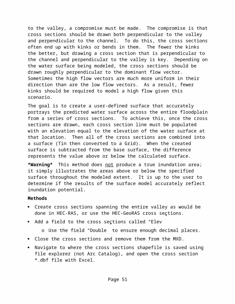
The grid should appear similar to the image above.Export the resulting ‘calculation’ file as a grid; cell size = 6
Open the resulting grid properties and change the symbology to stretched and a color ramp of blue.The grid should appear similar to the image above.
Create final Relative Water Surface Elevation Grid (RWSE)Each cell of the RWSE grid should contain values of zero at the water surface taken from the Bare Earth grid and range from the greatest elevation difference above and below the extracted water surface elevation (e.g. zero at the water surface to six feet of bathymetry below the water and hundreds of feet of topography above the water.)
Spatial Analyst – Raster Calculator (Subtract Raster_WSE from LiDAR)Expand the calculator[Choose the ‘Float’ Arithmetic function]
Page 52

[Choose the Bare Earth grid first, subtraction, then choose the new wse grid][Evaluate]The calculation should look as follows: Float([LiDAR]-[new wse])
Save new Relative Water Surface Elevation grid Right click on the calculation grid in the Table of Contents and select “Make Permanent”
Or, because there is always more than one way...Arc Toolbox3D Analyst Tools|Raster Math|MINUSChoose Bare Earth and raster input 1|Choose new WSE grid as raster input 2Out put new RWSE grid
The grid should appear similar to the image above.
Page 53

Classify and Ramp SymbologyOpen the RWSE grid properties|symbology|Show as Classified|Choose classification method as ‘defined interval’
Choose ‘exclusion’ to minimize the relative elevations to the floodplainExclude values above the desired range of elevations relative to channel migration.
Color ramp light blue to dark blueThe grid should appear similar to the image below.
Page 54

Explore the grid for accuracy.
For example, change the color of zero (theoretically the water surface) to bright yellow to see if the Relative Water Surface Elevation grid values reflect the true water surface.
Page 55

Appendix C. Data Reduction Forms
Page 56

Form 1: Summarized information for general mapping description and / or maps, photosReaches Description
River Miles if available or other descriptor of location
Length (ft or m)
Existing infrastructure
Channel movement barriers 4
Ecological value/critical habitat
Reach gradient (TTools or other GIS extraction method)
Channel width (ft or m) (Ttools or ArcGIS Analyst near distance tool)
Channel planform
Sinuosity
Valley width (ft or m)
Valley type5
Valley configuration
Valley geology
Floodplain features
Floodplain geology/soil type
Terrace features
Terrace geology/soil type
Bank material6
Sandy soils (sand > 35%) as a % of floodplain/banks
Clay soils (clay>15%) as a % of floodplain/banks
Sediment sources7
Form 2: Still in review. Will be submitted when finished.
4 Those meeting requirements in WAC 5 Glacial trough, post-glacial valley, lowland, underfit6 If known or can be determined by existing aerial or on ground photos or soil composition7 See if the Puget Sound watershed characterization provides adequate information or information from Lee Benda and Dan Miller
Page 57

Page 58

Appendix D. Glossary, Acronyms, and AbbreviationsGlossaryChannel migration: Channel migration is a natural process associated with streams8. Streams may migrate across valleys due to a variety of processes including channel and bank erosion processes, meander chute cutoff, avulsion, and vertical movement. The channel migration zone represents the area within which a given stream may migrate over time and includes avulsion hazard and erosion hazard zones (Rapp and Abbe 2003).
Datum is a surface or point relative to which measurements of height and/or horizontal position are reported. A vertical datum is a horizontal surface used as the zero point for measurements elevation; a horizontal datum is a reference for positions given in terms of latitude-longitude, State Plane coordinates, or Universal Transverse Mercator (UTM) coordinates.
Instantaneous Annual Peak Flow: The maximum instantaneous peak discharge, that is the highest discharge at an instant in time in a water year.
Parameter: A physical, chemical or biological property whose values determine environmental characteristics or behavior.
Reach: A specific portion or segment of a stream.
Recurrence interval (return period): The average interval of time within which the given flood will be equaled or exceeded once (USGS).
Regime: 1) "Regime theory" is a theory of the forming of channels in material carried by the streams. As used in this sense, the word "regime" applies only to streams that make at least part of their boundaries from their transported load and part of their transported load from their boundaries, carrying out the process at different places and times in any one stream in a balanced or alternating manner that prevents unlimited growth or removal of boundaries. 2) A stream, river, or canal of this type is called a "regime stream, river, or canal." A regime channel is said to be "in regime" when it has achieved average equilibrium; that is, the average values of the quantities that constitute regime do not show a definite trend over a considerable period--generally of the order of a decade. In unspecialized use "regime" and "regimen" are synonyms (USGS).
Regimen of a stream: The system or order characteristic of a stream; in other words, its habits with respect to velocity and volume, form of and changes in channel, capacity to transport sediment, and amount of material supplied for transportation. The term is also applied to a stream which has reached an equilibrium between corrosion and deposition or, in other words, to a graded stream (USGS).
Riparian: Relating to the banks along a natural course of water.
Streamflow: Discharge of water in a surface stream (river or creek).
8 The term stream encompasses all sizes of flowing water bodies.
Page 59

Surface waters of the state: Lakes, rivers, ponds, streams, inland waters, salt waters, wetlands and all other surface waters and water courses within the jurisdiction of Washington State.
Water Year: In Washington, the water year is the 12-month period extending from October 1 through September 30. The water year is designated by the calendar year in which it ends and which includes 9 of the 12 months. Thus, the year ended September 30, 1959, is called the "1959 water year."
Watershed: A drainage area or basin in which all land and water areas drain or flow toward a central collector such as a stream, river, or lake at a lower elevation.
Acronyms and AbbreviationsFollowing are acronyms and abbreviations used frequently in this report.
e.g. For example
Ecology Washington State Department of Ecology
EPA U.S. Environmental Protection Agency
et al. And others
GIS Geographic Information System software
GPS Global Positioning System
i.e. In other words
QA Quality assurance
RM River mile
SMA Shoreline Management Act
SMP Shoreline Master Program
SOP Standard operating procedures
USGS U.S. Geological Survey
WAC Washington Administrative Code
WDFW Washington Department of Fish and Wildlife
WRIA Water Resource Inventory Area
Units of Measurement
cfs cubic feet per second
cms cubic meters per second, a unit of flow.
ft feet
Page 60

kcfs 1000 cubic feet per second
kg kilograms, a unit of mass equal to 1,000 grams.
km kilometer, a unit of length equal to 1,000 meters.
m meter
mm millimeter
Page 61


