Download - © Michael Ruetz 2019

VIX Futures Return Decomposition
A THESIS SUBMITTED TO THE FALCULTY OF THE GRADUATE SCHOOL OF
THE UNIVERSITY OF MINNESOTA
By
Michael Ruetz
IN PARTIAL FULFILLMENT OF THE REQUIREMENTS FOR THE DEGREEE OF
MASTER OF SCIENCE
Glenn Pederson, Adviser
June 2019

© Michael Ruetz 2019

i
Abstract
VIX futures contracts have produced negative returns. I develop a method to decompose
the daily returns of VIX futures contracts in to the return components of roll down and
level. I show that roll down is the largest contributor to the negative returns. The return
decomposition analysis is carried out across the VIX futures term structure which
includes the one- to six-month VIX futures contracts. I use time series regressions to
estimate the beta coefficients of the return components relative to the VIX. The results of
the regression analyses are used to create a VIX curve strategy that is combined with the
S&P 500 Index.
ii
Table of Contents
List of Tables……………………………………………………………………………..iii
List of Figures…………………………………………………………………………….iv
Chapter 1: Introduction……………………………………………………………………1
Chapter 2: Data…………………………………………………………….…………….13
Chapter 3: Methods………………………………………………………………………35
Chapter 4: Results………………………………………………………………………..45
Chapter 5: Application…………………………………………………………………...54
Chapter 6: Summary and Conclusion……………………………………………………62
Bibliography…………………………………………………………………………… 66
Appendix ………………………………………………………...…………………...69

iii
List of Tables
Table 2.1: Average Daily Slopes between VIX and VIX Futures Contracts…………….14
Table 2.2: Statistical Characteristics of Daily Returns for VIX and VIX Futures
Contracts…………………………………………………………………………………20
Table 2.3: Daily Returns and Standard Deviation of the One-Month, Three-Month, and
Five-Month VIX Futures Contract Ranged by VIX Quintile……………………………24
Table 2.4: VIX Futures Cumulative P&L………………………………………………..27
Table 4.1: Regression Results for VIX and VIX Futures………………………………..47
Table 4.2: Eigenvectors and Percent of Variance Explained from PCA with VIX Returns
and Total Returns of One- to Six-Month VIX Futures Contracts………………………..52
Table 5.1: Results from Regressing the Daily Returns of the Three-Month VIX Futures
Contract on the One-Month VIX Futures Contract…………………………………...…58
Table 5.2: Risk and Return Statistics for the S&P 500 Index, VIX Strategy, and Portfolio
Strategy…………………………………………………………………………………..59
Table B.1: Statistical Characteristics of Daily Returns for VIX and VIX Futures
Contracts………………………………………………………………...……………….70
Table B.2: VIX Futures Cumulative P&L……………………………………………….71
Table D.1: Correlation Matrix Derived from Daily Returns…………………………….76

iv
List of Figures
Figure 1.1: Average Daily VIX and VIX Futures Closing Prices………………………...7
Figure 2.1: Average, Maximum, and Minimum Daily Closing Prices for VIX and
Constant nth Month VIX Futures Contracts……………………………………………..17
Figure 2.2: Plot of the Autocorrelations for the VIX Daily Return……………….……..31
Figure 2.3: Plot of the Autocorrelations for the Daily One-Month VIX Futures Roll Down
Return…………………………………………………………………………….………32
Figure 2.4: Plot of the Autocorrelations for the Daily One-Month VIX Futures Level
Return…………………………………………………………………………………….33
Figure 2.5: Plot of the Autocorrelations for the Daily One-Month VIX Futures Total
Return…………………………………………………………………………………….34
Figure 4.1: Proportion of Variance Explained by Each Principal Component…………..51
Figure C.1: Plot of the Partial Autocorrelations for the VIX Daily Returns..…………...72
Figure C.2: Plot of the Partial Autocorrelations for the Daily One-Month VIX Futures
Roll Down Return………………………………………………………………………..73
Figure C.3: Plot of the Partial Autocorrelations for the Daily One-Month VIX Futures
Level Return……………………………………………………………………………...74
Figure C.4: Plot of the Partial Autocorrelations for the Daily One-Month VIX Futures
Total Return…………………………………………………………………...…………75

1
Chapter I
Introduction
In Chapter 1 I review the Chicago Board Options Exchange’s Implied Volatility
Index (VIX) and VIX futures. I discuss the mechanics and pricing of each and provide
context regarding the historical performance of VIX futures contracts. I also provide
several theoretical explanations for the implied volatility term structure and discuss how
the VIX futures term structure has negatively impacted the performance of VIX futures
contracts. I conclude by discussing how this paper extends the current literature
regarding the performance attribution of VIX futures contracts.
1.1 Implied Volatility Index (VIX)
The price of an options contract is derived in a model, and the required model
inputs include price of the underlying, strike price, number of days until expiration,
interest rate, and implied volatility. Of the option pricing model inputs, option implied
volatility is the only variable that is inferred from the option’s price and is not directly
observed. Option implied volatility is the market’s expectation for the realized volatility
of the underlying asset from the current period until expiration of the options contract
(Natenberg, 2014). For example, the 30-day implied volatility of an at-the-money S&P
500 Index options contract is the market’s expectation for the realized volatility of the
S&P 500 Index over the next 30-days.
In finance it is a stylized fact that options contracts traded on financial assets,
such as equities and bonds, have implied volatilities that on average exceed the realized
volatility of the underlying asset (Coval and Shumway, 2001). The difference between

2
the implied volatility embedded in an options contract price and the subsequent realized
volatility is called the volatility risk premium (i.e. realized volatility minus implied
volatility). Bakshi and Kapadia (2003) find that a negative volatility risk premium exists
for buyers of equity index options and the premium is the price option investors are
willing to pay away to protect their equity position.
Equity market implied volatility generally increases when equity prices decline.
That has been especially true during periods of sharp equity market price declines, as
market participants expect higher realized volatility in the future which leads to higher
implied volatilities. The inverse price relationship between the S&P 500 Index and the
VIX is evident from their observed historical negative return correlation. The negative
correlation of returns between the S&P 500 Index and the VIX highlights why owners of
equity securities who are concerned about price declines might have a desire to own the
VIX or a VIX-related derivative contract.
The Chicago Board Options Exchange (CBOE) introduced the CBOE Implied
Volatility Index (VIX) in 1993 to provide a timely and consistent measure of equity
market implied volatility. Today, the VIX is widely quoted in the media and is often
used to gauge the market’s expectation for future realized volatility.
Originally, the VIX represented the 30-day implied volatility for the S&P 100
Index and was derived from exchange-traded S&P 100 Index option contracts. In 2003,
the CBOE, in conjunction with Goldman Sachs, modified the VIX calculation
methodology to reflect the 30-day implied volatility for the S&P 500 Index using price
information from CBOE-traded S&P 500 Index option contracts. The VIX calculation

3
methodology was enhanced in 2014 to include price information from S&P 500 Index
weekly option contracts.
The VIX price is quoted as the S&P 500 Index 30-day implied volatility
(annualized). The VIX is calculated from the prices of CBOE S&P 500 Index put and
call contracts that have more than 23 days but less than 37 days to expiration. To
maintain a constant 30-day implied volatility, the VIX calculation proportionally weights
one-month and two-month option contracts. The proportion changes each week.1
The option contracts used to calculate the VIX include CBOE out-of-the-money
(OTM) puts and calls on the S&P 500 Index. The center strike price of the puts and calls
is the strike price that sits just below the calculated forward S&P 500 Index price. Option
contracts with a zero-bid price are excluded from the VIX calculation and the number of
different strike prices used in the calculation is limited by the number of consecutive
strike prices with a non-zero bid price. The VIX price-squared is equal to the 30-day
variance swap rate (Zhang et al., 2010).
A unique characteristic of the VIX relative to other indices is that the VIX is not
directly investable since a VIX cash market does not exist. The reason for a nonexistent
VIX cash market is due to the cost prohibitive nature of replicating the VIX, which would
require buying and selling OTM puts and calls that are generally less liquid and have
wide bid-ask spreads. Transacting in a market with wide bid-ask spreads usually results
in outsized trading costs. For example, Buetow and Henderson (2016) find that the
average bid-ask spread for OTM S&P 500 Index puts and calls traded on the CBOE are
46.2% and 50.5% (bid-ask spread as percentage of midpoint price), respectively. Their
1 Refer to the equation in Appendix A for VIX calculation details.

4
research shows that buying OTM options at the offer price and then selling them at the
bid price, ceteris paribus, would result in a 50% loss in value. Furthermore, since the
VIX is a measure of constant 30-day implied volatility, the options used in the calculation
are continually changing as time passes. This implies that several transactions would be
required monthly to replicate the VIX.
In March 2004, the CBOE launched trading of VIX futures contracts. VIX
futures contracts are listed and traded electronically on the CBOE Futures Exchange (the
Exchange). The Exchange lists nine consecutive monthly futures contracts and six
consecutive weekly futures contracts. Each contract price is quoted as the forward S&P
500 Index 30-day implied volatility (annualized). For example, the price of a VIX
futures contract with three months remaining until expiration is the market expectation
for the S&P 500 Index 30-day implied volatility three months from now.
The notional value of each futures contract is equal to the futures contract price
multiplied by $1,000 and the minimum price interval is 0.05 points which is equal to $50.
On the day of expiration, the expiring VIX futures contract is cash-settled and will settle
at VIX spot based on the opening trades of the S&P 500 Index option contracts used in
the VIX calculation. The expiration date for the expiring monthly VIX futures contract is
30-days prior to the third Friday of the month immediately following the contract month.2
Since their inception, VIX futures have experienced a dramatic increase in trading
volume and open interest. The average daily volume of the one-month VIX futures
contract increased over 500 times and the total open interest of all listed VIX futures
contracts increased over 600 times (from March 2004 to June 2017). On December 4,
2 http://cfe.cboe.com/cfe-products/vx-cboe-volatility-index-vix-futures/contract-specifications

5
2017, the total outstanding notional amount of all VIX futures contracts listed was
approximately $8.1 billion, which compares to a total notional amount of approximately
$20.1 million on March 31, 2004.
A unique feature of the VIX futures contracts, relative to other markets that offer
futures contracts, is that a VIX cash market does not exist. The absence of a VIX cash
market diminishes the relationship between the price of the VIX and VIX futures
contracts since market participants are not able to execute cash and carry trades.3 The
lack of a cash VIX market also contributes to a wider VIX basis.4 Buetow and
Henderson (2016) point out that during extreme market events the difference in prices
(and returns) between the VIX and the first and second month VIX futures contracts can
be explained by the lack of a VIX cash market.
The financial performance of VIX futures contracts can be evaluated from either
the change in price and associated dollar profit and loss or percentage change in price (or
return). For example, consider a VIX futures contract that changes in price from 10 at
time t to 10.50 at time t+1. The change in price and profit is 0.50 and $500, respectively,
and the percentage change in price is equal to 5.0% (= 0.50/10).
During December 2009-December 2017, VIX futures experienced negative
average returns and the point on the VIX futures term structure with the sharpest declines
came from the one-month VIX futures contract. The leading contributor to the negative
returns of VIX futures contracts is the roll down. Roll down is the return that comes from
3 Cash and carry refers to buying (selling) a cash market instrument and simultaneously selling (buying) a
derivative instrument of the same market. The ability of market participants to engage in cash and carry
trades preserves the cash and theoretical derivatives pricing relationship. 4 Basis refers to the price differential between the cash price, or spot, and a futures contract of the same
market.

6
a change in price due to the VIX futures contract moving down the VIX term structure as
it approaches expiration. For example, when the VIX futures term structure is upward
sloping, the price of each futures contract declines with the passage of time as each
futures contract moves down the term structure. The magnitude of the price decline is
determined by the slope, or steepness, of the term structure. I define the slope as the
difference in price between two points on the term structure (e.g., the one-month VIX
futures price minus the two-month VIX futures price). The roll down return from an
upward sloping (contango) futures curve will be negative while the roll down from an
inverted (backwardated) futures curve will be positive holding all else constant.
The slope is most negative between the one-month and two-month VIX futures
contracts relative to all other term structure combinations using one- to six-month
contracts. For example, the daily average slope between the one- and two-month VIX
futures contracts is -0.9 versus a daily average slope of -0.2 for the five- and six-month
VIX futures contracts (during December 16, 2009-December 19, 2017).
The rounded cumulative compound return of the one-month VIX futures contract
is -100%. Other points on the term structure lost a similar amount with the three- and
five-month VIX futures contracts producing cumulative compound returns of -99.1% and
-95.3%, respectively. This research will show that most, if not all, of the negative return
of VIX futures contracts is accounted by the roll down.
1.2 VIX Term Structure
A VIX term structure exists and can be inferred from the price of VIX futures
contracts with different expirations or from S&P 500 Index option contracts using the

7
VIX calculation methodology and different expiration dates. Most of the time the VIX
term structure is upward sloping and is described by VIX spot having the lowest price
and each successive VIX futures contract with a longer time to expiration having a higher
price. An upward sloping VIX term structure is analogous to an upward sloping US
Treasury yield curve where the yield-to-maturity is greater for longer maturities.
VIX spot was lower than the price of the six-month VIX futures contract 92.6%
of the time with an average daily price differential of -4.4 (during December 2009-
December 2017). The graph below illustrates the average shape of the VIX term
structure by plotting and connecting the average daily VIX price with the average daily
VIX futures contract prices (during December 2009-December 2017).
Figure 1.1: Average Daily VIX and VIX Futures Closing Prices (December 2011 to December 2016)
There are various theoretical and empirical explanations for the shape of the
implied volatility term structure. The main explanations include the expectations

8
hypothesis, volatility mean reversion, and the risk premia of variance risk. The
theoretical concept of the expectations hypothesis is summarized well by Campa and
Chang (1995). They note that long-dated foreign currency implied volatility is equal to
the average of short-dated implied volatilities spanning the same time until expiration.
The expectations hypothesis postulates that an upward sloping implied volatility
term structure is explained by the market’s expectation for higher implied volatility in the
future. Mixon (2007) rejected the expectations hypothesis but found that the slope of the
implied volatility term structure was able to forecast short-dated implied volatility. After
correcting their model for the variance risk premium, the results improved but not enough
to satisfy the expectation hypothesis. An important insight from the research of Mixon
(2007) is that the implied volatility term structure is based on the risk neutral measure,
but real world implied and realized volatility is based on the objective measure.5 The
differences in the VIX term structure between the risk neutral and objective measures is
discussed by Nossman and Wilhelmsson (2009) and Simon and Campasano (2014).
Nossman and Wilhelmsson (2009) find stronger evidence of the expectations
hypothesis relative to Mixon (2007). They use VIX futures and conclude that the
expectations hypothesis holds for VIX futures over a 1-to-21-day forecasting horizon
after adjusting for the variance risk premium. The variance risk premium is negative and
is derived by estimating the risk neutral and objective parameters using a constant
elasticity stochastic variance model with jumps in the variance.6 The results show that
5 Options are priced from the risk neutral measure which imply arbitrage-free pricing, a complete market,
and discounted security values that follow a martingale process. Objective measures are probability
densities based on actual price innovations. 6 The constant elasticity stochastic variance model is a diffusion process with instantaneous volatility. The
model measures the mean reversion and instantaneous volatility of the variance process.

9
the variance risk premium is larger for long-dated option expirations when VIX spot is
high. Additionally, Nossman and Wilhelmsson (2009) find that the negative correlation
between VIX futures and the S&P 500 Index is enough to incentivize investors to pay a
variance risk premium for being long an instrument that will hedge S&P 500 Index
losses.
Using a normal inverse Gaussian maturity dependent risk premium model,
Huskaj and Nossman (2013) suggest that the variance risk premium for short-dated VIX
futures contracts is negative while being positive for long-dated contracts. This is
supported by showing that the beta7 and correlation of VIX futures contracts and VIX
declines as the time to expiration increases.
Johnson (2017) strongly rejects the expectations hypothesis for the VIX term
structure. He proposes that changes in the term structure are due to variation in the
variance risk premia embedded in the option contracts that are used to compute the VIX.
Johnson (2017) shows that longer maturity VIX contracts have smaller absolute Sharpe
ratios8 compared to the absolute Sharpe ratios of short-dated VIX contracts. This
indicates that variance risk is being priced differently at different maturities.
The differences in correlation between VIX futures contracts with different
expirations and VIX was also noted by Zhang et al. (2010). However, Zhang et al.
suggest that the VIX and VIX futures relationship can be established by modelling the
instantaneous variance using a square root, mean-reverting process with a stochastic
7 Slope coefficient estimated from an ordinary least squares regression. 8 Sharpe ratio is a measure of return per unit of standard deviation (
𝑟𝑖−𝑟𝑟𝑓
𝜎𝑖).

10
long-term mean level. Zhang et al. conclude that the term structure for VIX futures
volatility is downward-sloping and is explained by mean reversion of volatility.
Several previously written research papers have discussed the negative returns of
VIX futures contracts, and many have suggested the negative returns are due to the
upward sloping VIX futures term structure and the associated negative roll down.
However, very few papers in the existing literature attribute the daily returns of VIX
futures contracts to the two return components of roll down and level (changes in VIX).
Also, the existing literature does not provide an analysis of the return attribution for the
VIX futures term structure. The current literature focuses the return attribution on the
one-month VIX futures contract.
Alexander and Korovilas (2013) emphasize that in most market regimes the VIX
futures term structure is in contango and that has eroded the returns of exchange-traded
funds that buy and hold VIX futures contracts. Their research focuses on the early
redemption and front running issues associated with exchange-traded funds and
exchange-traded notes that trade VIX futures contracts. Buetow and Henderson (2016)
discuss why a cash VIX market does not exist and how that has led to a decoupling of
VIX and VIX futures pricing. They show that replicating a cash VIX market is cost
prohibitive due to the average illiquidity and wide bid-ask spreads of the out-of-the-
money options used in the VIX calculation.
Simon and Campasano (2014) study the VIX futures basis (slope) and assess its
ability to forecast changes in the VIX. Through their research they conclude that the VIX
futures basis was not able to predict changes in the VIX but was able to forecast changes
in the prices of VIX futures contracts. Using their research findings, they devise a

11
profitable trading strategy that buys and sells short VIX futures contracts. However, they
did not quantify how much the roll down return contributed to the negative returns of
VIX futures contracts.
The research conducted by Whaley (2013) finds that VIX futures contracts are
comprised of two return components, one relating to changes in VIX (level) and the other
being roll down. He shows that the calculation of roll down return is deterministic and is
quantified as the slope divided by the price of the constant maturity VIX futures contract
measured the previous day. Whaley provides summary statistics for the slope measured
at various points on the VIX futures term structure. While his work advances the
literature of decomposing the VIX futures returns, it does not provide an attribution
analysis for the VIX futures term structure.
1.3 Objective
Prior VIX futures research leaves open the question: how much do changes in
VIX level returns and roll down returns account for the realized returns of VIX futures?
My research proposes to help fill this gap by decomposing the daily returns of VIX
futures and attributing the returns to the return components (roll down and level).
My first research objective is to determine what proportion the roll down return
represents of the negative total return to VIX futures contracts. I plan to accomplish this
using daily VIX futures prices from the CBOE and developing a methodology for
decomposing and attributing the VIX futures returns. The expectation is that the roll
down return component can account for a large proportion of the negative returns of VIX
futures contracts.

12
The second objective of my research is to evaluate how returns, and return
components, vary across the VIX futures term structure. Specifically, I want to answer
the question: how do the total return and return components change for each contract on
the term structure relative to changes in VIX? I plan to use daily returns of the VIX and
the two return components (roll down and level) to conduct a regression analysis that
measures the sensitivity of each return component to changes in the VIX.
The third objective of my research is to evaluate whether the regression results
will allow me to construct a long-short VIX trading strategy using one-month and three-
month VIX futures contracts. More specifically, I want to determine if a VIX futures
curve strategy can be combined with a passive S&P 500 Index investment to create a
more efficient investment compared to the passive S&P 500 Index. I plan to evaluate the
dynamic nature of the estimated beta coefficients to determine the number of three-month
VIX futures contracts needed to hedge a single one-month VIX futures contract in
different market regimes.
1.4 Approach and Organization
In Chapter 2 I describe the data, calculations for each return component, and
provide summary statistics. In Chapter 3 I describe the time series regression model I use
to derive the sensitivities of each return component to the returns of the VIX. Chapter 4
is a discussion of the results from the regression and principal component models.
Chapter 5 provides the results of combining the S&P 500 Index returns with the returns
of a VIX futures curve strategy. In Chapter 6 I offer concluding comments and the
potential for future research.

13
Chapter II
Data
In this chapter I describe my original data by using basic statistical measures and
graphs. I then show and discuss how I decompose the total return of the VIX futures
contracts into two return components, roll down and level. I provide basic statistical
measures for the roll down and level returns and conclude by discussing the
autoregressive properties of the various return series.
2.1 VIX Futures Data
The analysis in this chapter is based on the daily total returns for the VIX and
VIX futures contracts. In addition, I analyze the daily returns of the VIX futures return
components, roll down and level. The total returns are calculated from the closing prices
of the VIX and monthly VIX futures contracts which are sourced from Excel data files
(file) posted by the CBOE on their website. Each file represents a single monthly VIX
futures contract and includes the daily open, close, high and low, and settlement prices. I
calculate the total returns and derive the returns of the return components for the one- to
six-month VIX futures contracts. Roll down and level returns are not calculated for the
VIX given that it is a spot price. All returns are calculated for the period of December
16, 2009 to December 19, 2017. The daily returns of each monthly VIX futures contract
are calculated from the settlement date of the prior contract up to and including the day
before the settlement date of the current contract.

14
2.2 The VIX Futures Term Structure
In chapter 1 I discuss that the price of a VIX futures contract represents the
expected VIX price, which is equivalent to the annualized 30-day implied volatility of the
S&P 500, at expiration of the VIX futures contract. For example, if on April 8, 2018 the
July VIX futures contract has a price of 19 this indicates the VIX is expected to be 19 on
July 18, 2018.
The VIX term structure is constructed from the closing prices of the VIX and each
VIX futures contract with expirations of one to six months. The shape of the term
structure is determined by the slope, or difference in price, between two points on the
term structure. In this analysis I measure the slope between each point on the term
structure starting with VIX and including each successive monthly VIX futures contract.
A steep term structure is characterized by large slopes between each point on the term
structure, whereas a flat term structure is distinguished by small to zero slopes between
each point. An inverted term structure is identified by VIX having the highest price on
the term structure and each successive VIX futures contract having a lower price.
Table 2.1: Average Daily Slopes Between VIX and VIX Futures Contracts (December 15, 2009 to
December 19, 2017)
VIX minus
1-month
1-month
minus
2-month
2-month
minus
3-month
3-month
minus
4-month
4-month
minus
5-month
5-month
minus
6-month
VIX Range
Average Slope -0.9 -1.1 -0.8 -0.6 -0.5 -0.4
Percent Negative Slope 84.2% 88.4% 91.7% 92.5% 92.6% 91.5%
Average Slope by VIX Level
VIX Level 1st Quintile -1.3 -1.3 -0.9 -0.7 -0.6 -0.5 9 to 13
VIX Level 2nd Quintile -1.2 -1.3 -0.9 -0.7 -0.5 -0.5 13 to 15
VIX Level 3rd Quintile -0.9 -1.3 -1.0 -0.7 -0.7 -0.6 15 to 17
VIX Level 4th Quintile -0.8 -1.4 -1.0 -0.7 -0.6 -0.5 17 to 21
VIX Level 5th Quintile -0.1 -0.4 -0.3 -0.2 -0.3 -0.2 21 to 48

15
Table 2.1 includes the average slopes and average slopes based on a quintile
ranking of the VIX price. I calculate the slope by subtracting from the closing price of
VIX, or a VIX futures contract, the closing price of the next month VIX futures contract.
For example, on January 18, 2013 the VIX closing price was 12.46 and the one-month
VIX futures contract closed at 14.65 which corresponds to a slope of -2.19. The average
slope is the arithmetic average of the daily slopes. I use Table 2.1 to illustrate that the
VIX term structure is upward-sloping and is steepest in the first couple of months.
The average slope can be used to compare the relative steepness between two
points on the term structure. In Table 2.1, observe that the average slope between the
one-month and two-month VIX futures contracts is -1.1 which is the most negative
among all the average slopes. The second most negative average slope (-0.9) is between
VIX and the one-month VIX futures contract. They compare to the negative average
slope of just -0.4 between the fifth and sixth month VIX futures contract. This highlights
that on average the front part of the VIX term structure (i.e., from VIX to the three-month
VIX futures contract) is steeper when compared to the rest of the term structure.
The Percent Negative Slope is the percentage of daily calculated slopes for a point
on the term structure that are negative. For example, the slope of the VIX and one-month
VIX futures contract is negative 84.2% of the time. Similarly, the four-month VIX
futures price is lower than the five-month VIX futures price 92.6% of the time. Each
highlighting that the VIX term structure is upward-sloping most of the time.
The price of VIX will influence the shape of the VIX term structure. This is
shown in the bottom half of Table 2.1 where the average slopes are provided based on a
quintile ranking of the VIX closing price. The average VIX closing price from the data

16
set is 17.11. When the VIX price is above its average, the VIX term structure becomes
relatively flat. Conversely, when the VIX is below its average the VIX term structure is
steeper.
When the VIX is between 9 and 13 the average slopes between VIX and the one-
month VIX futures contract (-1.3) and between the one-month and two-month VIX
futures contracts (-1.3) are more negative relative to the slopes between the other VIX
futures contracts. This illustrates that when the VIX closing price is well below its
average the VIX term structure becomes upward sloping and relatively steep. However,
when the VIX closing price is between 21 and 48 (fifth quintile) the average slope of the
VIX and one-month VIX futures contract (-0.1) is less negative than the slope between
the four- and five-month contracts (-0.3) highlighting that the VIX term structure
becomes flat (slope near zero) with above average VIX closing prices.
Figure 2.1 portrays the three possible shapes (relatively steep, relatively flat,
inverted) for the VIX term structure. These curves display the minimum, maximum, and
average prices for the VIX and VIX futures contracts that have a constant number of days
until expiration. I calculate the closing price of the constant nth month VIX futures
contract as,
𝐶𝑀𝑛,𝑡 =𝐷𝑡
𝑇𝑡∗ 𝐹𝑛,𝑡 +
𝑇𝑡−𝐷𝑡
𝑇𝑡∗ 𝐹𝑛+1,𝑡 , (1)
where, CMn,t is the closing price of the constant nth month VIX futures contract at time t,
Dt is the number of days remaining until the expiration of the one-month VIX futures
contract (including day t but not including the settlement date), Tt is the total number of
trading days of the current one-month VIX futures contract from the settlement date of

17
the prior one-month contract until one day prior to the current contract settlement date,
and Fn is the closing price of the nth month VIX futures contract.
Figure 2.1: Average, Maximum, and Minimum Daily Closing Price for VIX and Constant nth Month
VIX Futures Contracts (December 15, 2009 to December 19, 2017)
The line representing the maximum depicts an inverted term structure which is
identified by VIX having the highest closing price and the constant five-month VIX
futures contract having the lowest closing price. In most cases, an inverted VIX term
structure has been the result of large price declines for the S&P 500 Index. An inverted
VIX term structure is uncommon and one lasting more than a few months is quite rare.

18
2.3 Two-Component Return Calculation
A daily total return can be calculated for VIX and each VIX futures contract.
Additionally, the daily total return of each VIX futures contract can be decomposed into
two return components, roll down and level. The total return of VIX futures contract
over the interval [t-1, t] is given by,
𝑟𝑡 = 𝐹𝑛,𝑡
𝐹𝑛,𝑡−1− 1 =
𝑃𝑛,𝑡
𝐹𝑛,𝑡−1, (2)
where over the interval [t-1, t] the terms Fn and Pn denote the nth month VIX futures
closing price and change in price of the nth month VIX futures contract, respectively.
The multiperiod compounded return for k periods can be written as,
𝑟𝑡[𝑘] = (∏ (1 + 𝑟𝑡−𝑗)) − 1𝑘−1𝑗=0 , (3)
where 𝑟𝑡[𝑘] is the product of the k one-period returns.
The total return can be decomposed as,
𝑟𝑡 = 𝐶𝑟𝑡 + 𝐿𝑟𝑡 , (4)
where Crt and Lrt denote the roll down return and level return, respectively. More
specifically, I define the roll down return at time t as,
𝐶𝑟𝑡 =𝐶𝑛,𝑡
𝐹𝑛,𝑡−1, (5)

19
where the term Cn,t denotes the one day roll down of the nth VIX futures contract at time
t. The roll down of F1 is calculated relative to the closing price of VIX and for all other
VIX futures contracts (Fn+1), the roll down is calculated relative to an n-1 constant month
VIX futures closing price. I calculate the roll down at time t as,
𝐶𝑛,𝑡 = 𝐶𝑀𝑛−1,𝑡−1−𝐹𝑛,𝑡−1
𝐷𝑡, (6)
and where Dt is the number of trading days remaining until the expiration of F1 including
day t but not including the settlement date. The constant nth month VIX futures closing
price (𝐶𝑀𝑛,𝑡) is calculated as the daily proportion of the n and n+1 VIX futures closing
prices (as in equation 1).
I define the level return at time t as,
𝐿𝑟𝑡 = 𝑟𝑡 − 𝐶𝑟𝑡 . (7)
2.4 Characteristics of Return Series
In the following sections I provide and discuss the return characteristics of the
VIX and the one-, three-, and five-month VIX futures contracts. I leave out the results of
the two-, four-, and six-month VIX futures contracts to keep the results compact but
without detracting from the analysis.9 In Section 2.4.1 I highlight the characteristics of
the entire return series and then in Section 2.4.2 I segment the returns and return
characteristics based on a quintile ranking of the VIX price. In Section 2.5 I provide the
output of testing the various returns series for stationarity and autocorrelation.
9 Results for the two-, four-, and six-month VIX futures contracts are provided in Appendix B.
20
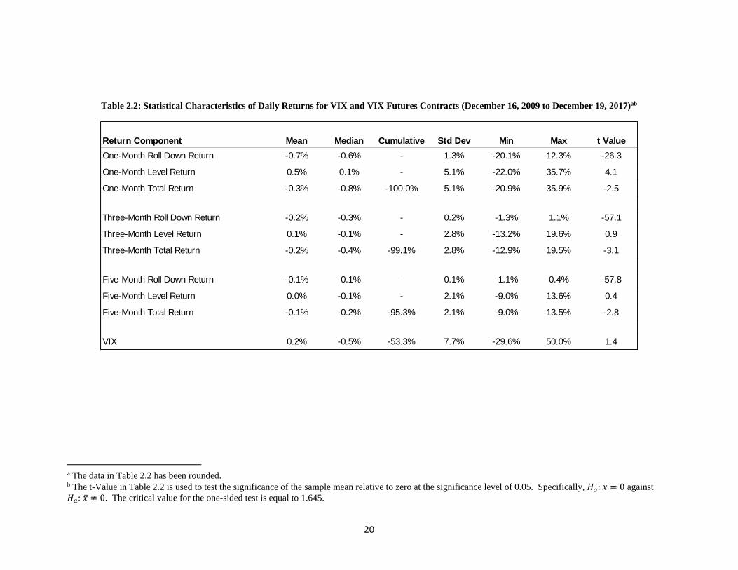
Table 2.2: Statistical Characteristics of Daily Returns for VIX and VIX Futures Contracts (December 16, 2009 to December 19, 2017)ab
a The data in Table 2.2 has been rounded. b The t-Value in Table 2.2 is used to test the significance of the sample mean relative to zero at the significance level of 0.05. Specifically, 𝐻𝑜: �̅� = 0 against
𝐻𝑎: �̅� ≠ 0. The critical value for the one-sided test is equal to 1.645.
Return Component Mean Median Cumulative Std Dev Min Max t Value
One-Month Roll Down Return -0.7% -0.6% - 1.3% -20.1% 12.3% -26.3
One-Month Level Return 0.5% 0.1% - 5.1% -22.0% 35.7% 4.1
One-Month Total Return -0.3% -0.8% -100.0% 5.1% -20.9% 35.9% -2.5
Three-Month Roll Down Return -0.2% -0.3% - 0.2% -1.3% 1.1% -57.1
Three-Month Level Return 0.1% -0.1% - 2.8% -13.2% 19.6% 0.9
Three-Month Total Return -0.2% -0.4% -99.1% 2.8% -12.9% 19.5% -3.1
Five-Month Roll Down Return -0.1% -0.1% - 0.1% -1.1% 0.4% -57.8
Five-Month Level Return 0.0% -0.1% - 2.1% -9.0% 13.6% 0.4
Five-Month Total Return -0.1% -0.2% -95.3% 2.1% -9.0% 13.5% -2.8
VIX 0.2% -0.5% -53.3% 7.7% -29.6% 50.0% 1.4

21
2.4.1 Basic Statistics
In Table 2.2 I display basic statistical characteristics for the daily total returns of
the VIX and VIX futures contracts as well as the two VIX futures return components.
VIX futures contracts with expirations of one, three, and five months are shown to
illustrate the differences in return statistics across the term structure.
In Table 2.2, the mean and median roll down returns are negative for each
monthly VIX futures contract. The average roll down returns of the one-month VIX
futures contract (-0.7%) are more negative than the average roll down returns of the
three- (-0.2%) and five-month (-0.1%) contracts, which supports the view that the VIX
term structure is on average upward sloping and steeper in the front-end. A futures
contract has a finite life and as the time to expiration approaches, the contract loses value
if an upward-sloping term persists. Hence, the negative return on an upward-sloping
term structure.
Unlike the average roll down returns, the average level returns are positive for
each monthly VIX futures contract. Although comparing the mean and median level
returns shows that the average level returns are pulled higher by the larger relative
changes in the price for VIX. For example, from December 16, 2009 to December 19,
2017 the average VIX price was 17.11 with a maximum price of 48 (180% from average)
and minimum price of 9.14 (47% from average). During the same period, the maximum
and minimum closing price, and average closing prices for the one-month VIX futures
contract were 45, 9.88 and 17.93, respectively.
The average level return of the one-month VIX futures contract (0.5%) compared
to the three- and five-month VIX futures contracts (0.1% and 0.0%) shows that the one-

22
month VIX futures contract has the greatest sensitivity to changes in the VIX price. This
is also supported by the large difference between the mean and median level returns of
the one-month VIX futures contract (0.5% versus 0.1%) relative to the difference in mean
and median level returns of the other two contracts.
The standard deviation of returns in Table 2.2 highlight that the total return
standard deviation for each monthly VIX futures contract is primarily accounted for by
the standard deviation of level returns. In fact, 96.6% of the total standard deviation of
the one-month VIX futures contract is accounted for by the level return component. I
calculate the percentage contribution of level return standard deviation to the total return
standard deviation as the covariance of level and total returns divided by the variance of
total returns. The reason that the level return standard deviation accounts for so much of
the total return standard deviation is due to the strong positive correlation between the
level and total returns (0.97) and the similar return standard deviations between the two
return components.
Since VIX is a spot price, it does not have a roll down return component and
therefore, it’s standard deviation of returns can be considered both level return and total
return standard deviation. The standard deviation of the level return declines starting
with VIX and as the time to expiration increases (i.e. each successive VIX futures
contract). For example, the VIX standard deviation of returns (7.7%) is 1.5 times greater
than the standard deviation of the one-month VIX futures contract level return (5.1%) and
more than 3.5 times the standard deviation of the five-month VIX futures contract level
return (2.1%). This shows that the term structure of realized volatility for the VIX and
VIX futures contracts is inverted. Zhang et al (2010) find similar results and conclude
23
that the downward sloping realized volatility term structure of VIX futures contracts is
explained by the volatility mean-reversion process.
The t-values shown in Table 2.2 are used to test the significance of the mean
return for each return component relative to zero. The one-tailed critical value at the 0.05
level is 1.645. All but the VIX, three-month level, and five-month level returns are
statistically different from zero at the 0.05 level. The t-values for the return components
of the one-, three-, and five-month VIX futures contracts highlight the relative magnitude
of loss from the roll down component and standard deviation of the level component.
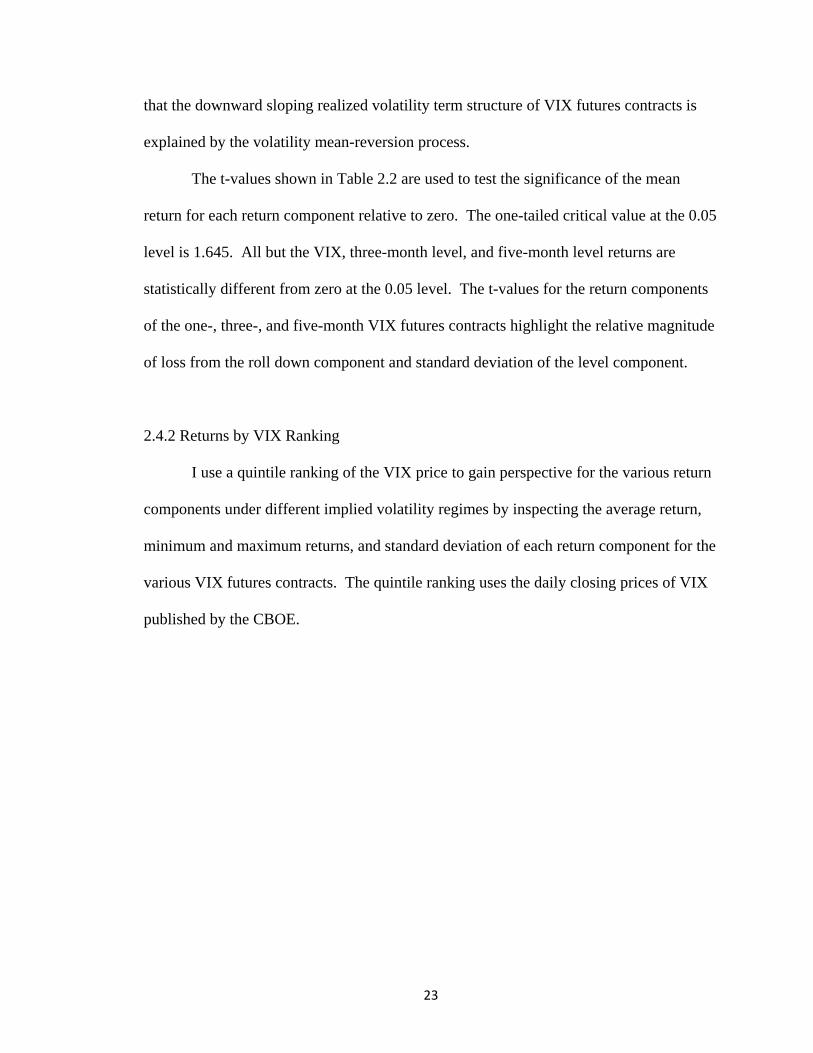
2.4.2 Returns by VIX Ranking
I use a quintile ranking of the VIX price to gain perspective for the various return
components under different implied volatility regimes by inspecting the average return,
minimum and maximum returns, and standard deviation of each return component for the
various VIX futures contracts. The quintile ranking uses the daily closing prices of VIX
published by the CBOE.

24
Table 2.3: Daily Returns and Standard Deviation of the One-Month, Three-Month and Five-Month VIX Futures Contracts Ranked by VIX Quintile
(December 16, 2009 to December 19, 2017)a
a The data in Table 2.3 has been rounded.
1-month Roll
Down Return
3-month Roll
Down Return
5-month Roll
Down Return
1-month Level
Return
3-month Level
Return
5-month Level
Return
1-month Total
Return
3-month Total
Return
5-month Total
ReturnVIX
First Quintile Avg Return -1.4% -0.3% -0.2% 0.2% -0.3% -0.2% -1.2% -0.6% -0.4%
Std Dev 1.5% 0.2% 0.1% 2.6% 1.6% 1.1% 2.7% 1.5% 1.1%
Min -20.1% -1.2% -0.7% -10.1% -11.1% -7.6% -19.3% -11.3% -7.6% 9.1
Max 0.3% 1.1% 0.0% 8.5% 4.0% 2.6% 6.1% 3.5% 2.3% 12.7
Second Quintile Avg Return -1.0% -0.3% -0.2% 0.0% -0.3% -0.3% -0.9% -0.6% -0.4%
Std Dev 1.1% 0.1% 0.1% 3.6% 1.8% 1.4% 3.4% 1.8% 1.4%
Min -10.2% -0.9% -1.1% -19.9% -7.9% -6.7% -16.5% -8.1% -6.7% 12.7
Max 3.4% 0.0% 0.0% 14.0% 4.1% 3.5% 14.1% 3.8% 3.1% 14.5
Third Quintile Avg Return -0.7% -0.3% -0.2% 0.1% -0.2% -0.1% -0.6% -0.4% -0.3%
Std Dev 1.2% 0.2% 0.1% 4.7% 2.6% 1.8% 4.8% 2.6% 1.8%
Min -10.7% -1.3% -0.8% -14.1% -7.6% -6.6% -13.1% -7.8% -6.7% 14.5
Max 12.3% 0.0% 0.0% 20.1% 10.5% 6.9% 32.4% 10.1% 6.8% 16.9
Fourth Quintile Avg Return -0.5% -0.3% -0.1% 0.6% 0.3% 0.1% 0.1% 0.0% 0.0%
Std Dev 0.9% 0.2% 0.1% 5.9% 3.1% 2.3% 5.8% 3.1% 2.2%
Min -8.9% -0.9% -0.5% -21.0% -12.8% -9.0% -20.9% -12.8% -9.0% 16.9
Max 3.8% 0.2% 0.0% 33.7% 10.6% 8.1% 31.0% 9.9% 7.8% 20.6
Fifth Quintile Avg Return -0.2% -0.1% -0.1% 1.3% 0.7% 0.6% 1.2% 0.7% 0.5%
Std Dev 1.2% 0.2% 0.1% 7.1% 4.0% 3.0% 7.1% 4.0% 3.0%
Min -7.3% -1.2% -0.8% -22.0% -13.2% -8.7% -16.8% -12.9% -8.7% 20.6
Max 5.2% 0.6% 0.4% 35.7% 19.6% 13.6% 35.9% 19.5% 13.5% 48.0
Roll Down Returns Level Returns Total Returns

25
The data in Table 2.3 offers some interesting insight regarding the characteristics
of the VIX term structure. For example, the large negative roll down returns of the one-
month VIX futures contract (-1.4%) compared with the negative roll down returns of the
three- (-0.3%) and five-month ( -0.2%) VIX futures contracts highlight the fact that the
front-end of the VIX term structure is generally steeper when the VIX is in the first
quintile (below 12.7) of its price history. However, when the VIX price is in the fifth
quintile (greater than 20.6) the average roll down returns of the one-month VIX futures
contract (-0.2%) is similar to the average roll down returns of the three- (-0.1%) and five-
month (-0.1%) VIX futures contracts. This illustrates the fact that the average VIX term
structure is flat when the VIX price is high.
The standard deviation and the range of roll down and level returns vary greatly
depending on the level of the VIX closing price. For example, the standard deviation of
the one-month level returns in the first quintile (2.6%) is less than half of the standard
deviation in the fifth quintile (7.1%). This demonstrates that the VIX is more volatile
when the VIX is above its average price.
Similarly, the range of level returns for the one-month contract significantly
expand between the first (18.6%) and fifth (57.7%) quintiles. However, the standard
deviation of the one-month roll down returns in the first quintile (1.5%) is slightly greater
than the fifth quintile (1.2%). And the range of roll down returns for the one-month
contract decline between the first (20.4%) and fifth (12.5%) quintiles. These results
support the view that the VIX term structure becomes flat when the VIX price is above its
average price of 17.11.

26
2.4.3 VIX Futures Profit and Loss
The returns shown previously are helpful in drawing conclusions about the total
return distribution of VIX futures contracts and return distributions for the roll down and
level return components. The cumulative profit and loss (P&L) from buying and holding
a VIX futures contract aid in illustrating the differences between the roll down and level
components.
I use Table 2.4 to show the cumulative profit and loss (P&L) from buying and
holding a one-, three-, and five-month VIX futures contract. Like the returns calculated
earlier, a buy-and-hold VIX futures strategy involves buying and holding the current
month contract up to and including one-day prior to the settlement date. On the day prior
to the settlement date, the buy-and-hold strategy sells the current contract at the closing
price and simultaneously buys the new month contract at the closing price.
The total, roll down, and level P&Ls are derived from equations 2, 6, and 7 and
are indicative of a buy-and-hold strategy with one VIX futures contract. For example,
during December 16, 2009 to December 19, 2017 the one-month VIX futures contract
lost 127.89 points or -$127,885 (-127.89*1,000). During the same period the roll down
component lost 228.753 points (-$228,753) and the level component gained 100.868
points ($100,868). The P&Ls shown in Table 2.4 are the summed daily P&Ls for each
component during December 16, 2009 to December 19, 2017 and for each component
from quintile one and five. The quintiles were determined by a quintile ranking of the
VIX price.
27
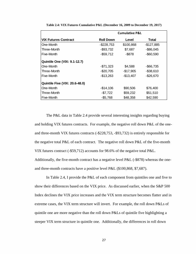
Table 2.4: VIX Futures Cumulative P&L (December 16, 2009 to December 19, 2017)
The P&L data in Table 2.4 provide several interesting insights regarding buying
and holding VIX futures contracts. For example, the negative roll down P&L of the one-
and three-month VIX futures contracts (-$228,753, -$93,732) is entirely responsible for
the negative total P&L of each contract. The negative roll down P&L of the five-month
VIX futures contract (-$59,712) accounts for 98.6% of the negative total P&L.
Additionally, the five-month contract has a negative level P&L (-$878) whereas the one-
and three-month contracts have a positive level P&L ($100,868, $7,687).
In Table 2.4, I provide the P&L of each component from quintiles one and five to
show their differences based on the VIX price. As discussed earlier, when the S&P 500
Index declines the VIX price increases and the VIX term structure becomes flatter and in
extreme cases, the VIX term structure will invert. For example, the roll down P&Ls of
quintile one are more negative than the roll down P&Ls of quintile five highlighting a
steeper VIX term structure in quintile one. Additionally, the differences in roll down
VIX Futures Contract Roll Down Level Total
One-Month -$228,753 $100,868 -$127,885
Three-Month -$93,732 $7,687 -$86,045
Five-Month -$59,712 -$878 -$60,590
Quintile One (VIX: 9.1-12.7)
One-Month -$71,323 $4,588 -$66,735
Three-Month -$20,705 -$17,905 -$38,610
Five-Month -$13,263 -$13,407 -$26,670
Quintile Five (VIX: 20.6-48.0)
One-Month -$14,106 $90,506 $76,400
Three-Month -$7,722 $59,232 $51,510
Five-Month -$5,768 $48,358 $42,590
Cumulative P&L

28
P&L between the monthly VIX futures contracts show that when the VIX price is low
(quintile one) the VIX term structure is steeper as illustrated by the greater roll down
losses.
The difference in level P&Ls between quintiles one and five highlight that the
level component produces the largest P&L when the VIX price is high. Additionally, the
level P&L is greater than the roll down P&L for each VIX futures contract in quintile
five. This finding implies that buying and holding a VIX futures contract when the VIX
price is at or above 20.6 results in a positive total P&L.
2.5 Stationarity and Autocorrelation of Returns
To evaluate the characteristics of the return series I assess the stability of the
mean and variance as well as correlation of returns with respect to time. A return series
that exhibits a mean and variance that is invariant with time and where the covariances
between xt and xt+h only depend on the distance between them is considered covariance
stationary. Covariance stationary time series offer a greater ability to make inferences
regarding future observations.
Time series regression analysis relies on a covariance stationary process in the
residuals. If the data series are not covariance stationary, or adjusted to be covariance
stationary, then the estimated variance of the regression coefficient(s) can be biased
leading to invalid t-statistics. For example, an independent variable that has a positive
autocorrelated series can result in an underestimation of the beta coefficient variance,
leading to overstated t-statistics. In finance it is common to assume that return series are
covariance stationary since the derived returns are a form of detrending transformation.

29
However, using return series does not jettison the need to check and possibly correct the
time series regression model for autocorrelated or heteroskedastic residuals.
In this section I discuss the results of the Augmented Dicky Fuller (ADF) unit
root test for stationarity in the daily returns of the VIX, and the daily total returns and
returns of each return component (roll down and level) for the one-month, three-month,
and five-month VIX futures contracts. Additionally, I present the autocorrelation test
results for the returns of the VIX and one-month VIX futures contract. The partial
autocorrelation test results are provided in Appendix C.
The ADF test is conducted for the VIX returns and the various returns (total, roll
down, level) of the VIX futures contracts. The ADF test includes a test of the null
hypothesis of a unit root (𝐻0: 𝛾 = 0) versus the alternative hypothesis (𝐻𝑎: 𝛾 < 0). The
equation for the ADF-test statistic can be written as,
𝐴𝐷𝐹 𝑡𝑒𝑠𝑡 = �̂�−1
𝑠𝑡𝑑(�̂�), (8)
where �̂� is estimated in a least-squares regression (Tsay, 2010, pp. 77). The estimating
equation is written as,
∆𝑦𝑡 = 𝜇 + 𝛽𝑡 + 𝛾 ∗ 𝑦𝑡−1 + ∑ ∅𝑖𝑝−1𝑖=1 ∆𝑦𝑡−𝑖 + 휀𝑡 , (9)
where ∅𝑖 = − ∑ 𝛾𝑘𝑝𝑘=𝑖+1 , 𝛾 ∗= (∑ 𝛾𝑖) − 1,
𝑝𝑗=1 and ∆𝑦 is the daily change in y (the total
return or return component).
Since each time series is comprised of daily derived returns, stationarity is not an
issue as most return series are covariance stationary. In fact, the ADF test for the returns
of the VIX and VIX futures contracts confirm this with each test result rejecting the null
30
hypothesis (non-stationary) for the alternative hypothesis (stationary) at all levels of
significance.
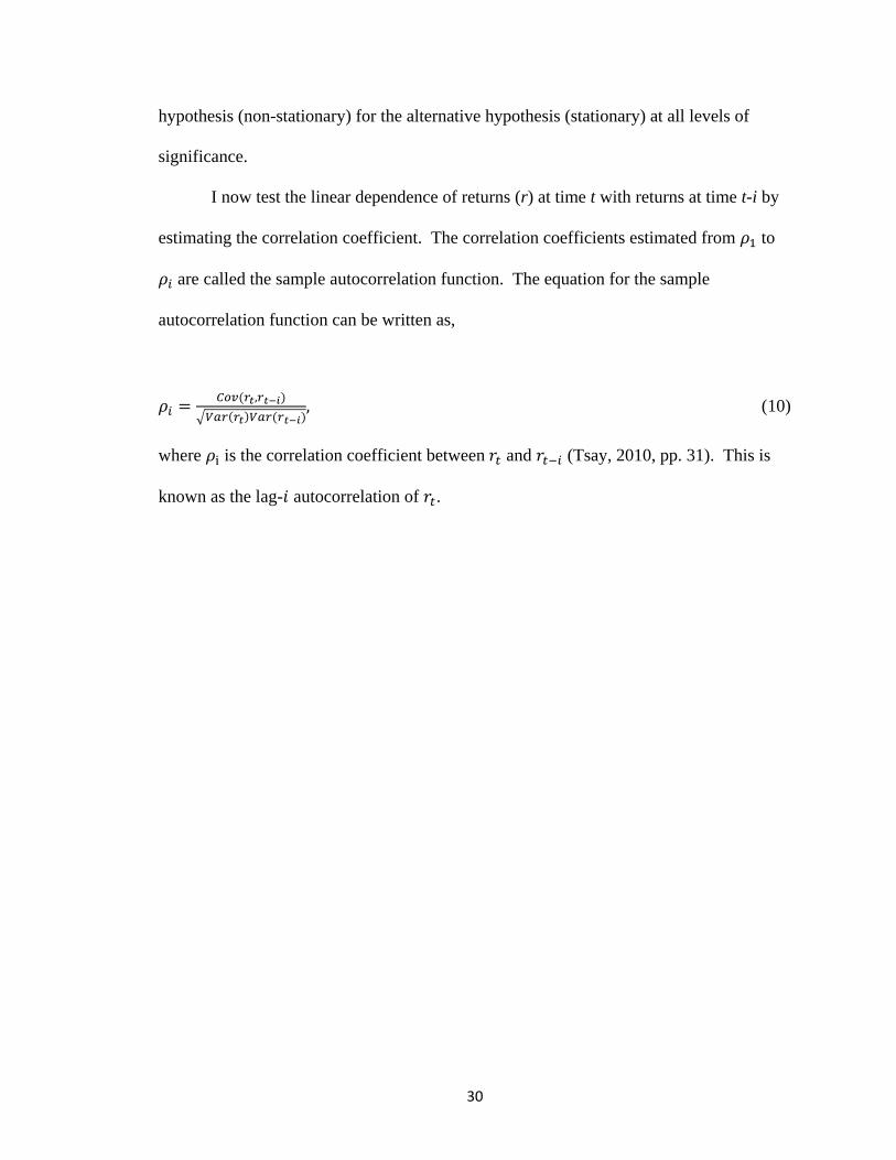
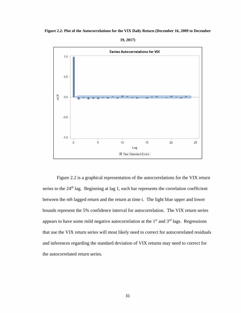
I now test the linear dependence of returns (r) at time t with returns at time t-i by
estimating the correlation coefficient. The correlation coefficients estimated from 𝜌1 to
𝜌𝑖 are called the sample autocorrelation function. The equation for the sample
autocorrelation function can be written as,
𝜌𝑖 =𝐶𝑜𝑣(𝑟𝑡,𝑟𝑡−𝑖)
√𝑉𝑎𝑟(𝑟𝑡)𝑉𝑎𝑟(𝑟𝑡−𝑖), (10)
where 𝜌i is the correlation coefficient between 𝑟𝑡 and 𝑟𝑡−𝑖 (Tsay, 2010, pp. 31). This is
known as the lag-𝑖 autocorrelation of 𝑟𝑡.
31
Figure 2.2: Plot of the Autocorrelations for the VIX Daily Return (December 16, 2009 to December
19, 2017)
Figure 2.2 is a graphical representation of the autocorrelations for the VIX return
series to the 24th lag. Beginning at lag 1, each bar represents the correlation coefficient
between the nth lagged return and the return at time t. The light blue upper and lower
bounds represent the 5% confidence interval for autocorrelation. The VIX return series
appears to have some mild negative autocorrelation at the 1st and 3rd lags. Regressions
that use the VIX return series will most likely need to correct for autocorrelated residuals
and inferences regarding the standard deviation of VIX returns may need to correct for
the autocorrelated return series.

32
Figure 2.3: Plot of the Autocorrelations for the Daily One-Month VIX Futures Roll Down Return
(December 16, 2009 to December 19, 2017)
Figure 2.3 illustrates the autocorrelations for the roll down returns of the one-
month VIX futures contract. These returns are highly autocorrelated and the return series
follows an autoregressive process with lags 1 through 10 positive and significant at the
5% level. The partial autocorrelations for lags 1, 3, and 5 are significant at the 5% level
indicating that the autoregressive process is driven by the first few lags. The residuals of
any time series regression analysis using the one-month VIX futures roll down returns
will need to be carefully examined and corrected for autocorrelation. Otherwise, the
variance of the estimated beta coefficient will be misstated leading to invalid t-statistics.
Additionally, the one-month VIX futures roll down return series should be corrected for
autocorrelation before inferences regarding the standard deviation are made.

33
Figure 2.4: Plot of the Autocorrelations for the Daily One-Month VIX Futures Level Return
(December 16, 2009 to December 19, 2017)
Figure 2.4 illustrates the autocorrelations for the one-month VIX futures level
return series. The return series appears to have mild negative autocorrelation at the 1st
and 5th lag that is significant at the 5% confidence level. Any inference the standard
deviation of returns or regression results for the one-month VIX futures level return may
need to be corrected for autocorrelation.

34
Figure 2.5: Plot of the Autocorrelations for the Daily One-Month VIX Futures Total Return
(December 16, 2009 to December 19, 2017)
Figure 2.5 illustrates the autocorrelations for the total returns of the one-month
VIX futures contract. The total return series of the one-month VIX futures contract does
not appear to be autocorrelated given that none of the correlation coefficients for the lags
are statistically different from zero. Therefore, the one-month VIX futures contract total
return series is considered covariance stationary. Although it is interesting to note that
the roll down and level returns of the one-month VIX futures contract were not
covariance stationary as shown in Figures 2.3 and 2.4.

35
Chapter III
Methods
I begin Chapter 3 by discussing the assumptions of a time series regression model.
I discuss covariance stationarity and highlight its importance with the asymptotic
properties of a least squares regression. Next, I review and provide details for the
univariate regression models that will be estimated. I conclude Chapter 3 by providing
my expectations for the output of the regression models.
3.1 Time Series Regression Model
Time series regression models are used extensively in economics and finance to
identify and explain the relationship between variables that are indexed by time. An
example of a time series regression model in finance is one that uses the returns of the
S&P 500 Index to explain the returns of a long/short equity hedge fund. Here, the returns
of the long/short equity hedge fund represent the dependent variable and the returns of
the S&P 500 Index represent the explanatory variable. Using this simple example, the
time series least squares regression model can be written as,
𝑦𝑡 = 𝛼 + 𝛽𝑥𝑡 + 𝑢𝑡 ,
where y is the return of the long/short equity hedge fund at time t, x is the return of the
S&P 500 Index at time t, 𝛽 is the estimated beta coefficient, and 𝑢 is the error term.
There are five assumptions that must hold for the estimated beta coefficient to be
the best linear unbiased estimator (𝛽) of the regression. The term “best” has the meaning

36
minimum variance and unbiased means that the estimates are unbiased across all time
periods (Wooldridge, 2013).
The first assumption of a time series regression model is that the model
parameters are linear. The second assumption necessitates that the independent variables
are not constant and are not perfectly correlated. The third assumption of a time series
regression model requires that the expected value of the error term, u, is zero for all time
periods. Assumption four imposes that the variance of error term is constant across all
time periods and assumption five requires that the error term be serially uncorrelated. If
only assumptions one, two, and three hold then the time series regression estimator, β, is
considered unbiased but is not considered the best linear unbiased estimator (Wooldridge,
2013).
The law of large numbers and central limit theorem applied to cross-sectional data
can be applied to time series data through sample averages and covariance stationarity.
As discussed in 2.4.3, a return series (rt) is said to be covariance stationary if both the
mean and variance of rt are time invariant and the covariance between rt and rt-h, where h
is an arbitrary integer, only depends on h. Covariance stationarity requires that the
correlation between rt and rt-h goes to zero sufficiently quickly as h increases. As we will
see, covariance stationarity is required for asymptotically valid regression results (Tsay,
2010).
As the size of the return series (T) goes to infinity, asymptotic distribution theory
can be used to describe the first and second moments (parameter estimates) of the
dependent and explanatory variables. The probability limit (e.g., 95% probability) that
the sample parameter estimates of the dependent and explanatory variables converge to

37
their true parameter estimates can be achieved with a sufficiently large T. When the
probability limit is reached, the parameter estimates are considered consistent. Although
a return series can be serially correlated, the sample parameter estimates can converge to
the true parameter estimates based on the probability limit provided the return series is
covariance stationary (Hamilton, 1994).
The first assumption of a time series regression model, linearity, is enhanced by
requiring that the independent and dependent variables be covariance stationary. The
third assumption of the time series regression model is relaxed by requiring that the
independent variable is contemporaneously exogenous. The fourth assumption is relaxed
so that the requirement is for contemporaneous homoskedastic errors conditioned on the
independent variable at time t. The assumptions of no perfect collinearity among the
independent variables and zero correlation in the errors across time remain. Provided the
time series regression model can meet these assumptions, the beta coefficient estimates
are consistent, and the various inferences (e.g., t-statistics, F-statistics) are asymptotically
valid (Wooldridge, 2013).
3.2 Model Estimation
I use univariate time series regressions to estimate the daily total returns and
return components, roll down and level, for the one-, three-, and five-month VIX futures
contracts based on contemporaneous daily returns of the VIX. Additionally, I use
univariate time series regressions to estimate the daily returns of VIX from
contemporaneous daily total returns of the S&P 500 Index. Three equations are

38
estimated for each VIX futures contract and one is estimated for the VIX, which yields
ten regression models estimated in total. The first set of equations are written as,
𝑂𝑉𝐹𝑖,𝑡 = 𝛼𝑖 + 𝛽𝑂𝑖𝑉𝐼𝑋𝑡 + 𝜖𝑖,𝑡 , (11)
where t is the counter for time and i=1,2,3 represents daily total return (1), roll down
return (2), and level return (3) of the one-month VIX futures contract (OVF), 𝛼𝑖 is the
intercept of the regression equation, 𝐵𝑂𝑖 is the beta coefficient, and 𝑉𝐼𝑋𝑡 is the daily
return of the VIX. The second set of equations are written as,
𝑇𝑉𝐹𝑗,𝑡 = 𝛾𝑗 + 𝛽𝑇𝑗𝑉𝐼𝑋𝑡 + 𝜖𝑗,𝑡 , (12)
where t is a counter for time and j=1,2,3 represents daily total return (1), roll down return
(2), and level return (3) of the three-month VIX futures contract (TVF), 𝛾𝑗 is the intercept
of the regression equation, 𝐵𝑇𝑗 is the beta coefficient, and 𝑉𝐼𝑋𝑡 is the daily return of the
VIX. The third set of equations are written as,
𝐹𝑉𝐹𝑘,𝑡 = 𝛿𝑘 + 𝛽𝐹𝑘𝑉𝐼𝑋𝑡 + 𝜖𝑘,𝑡 , (13)
where t is a counter for time and k=1,2,3 represents daily total return (1), roll down return
(2), and level return (3) of the five-month VIX futures contract (FVF), 𝛿𝑘 is the intercept
of the regression equation, 𝐵𝐹𝑘 is the beta coefficient, and 𝑉𝐼𝑋𝑡 is the daily return of the
VIX. The final set of equations are written as,
𝑉𝐼𝑋𝑡 = 𝜃𝑣 + 𝛽𝑣𝑆𝑃𝑋𝑡 + 𝜖𝑣,𝑡 , (14)
39
where 𝑉𝐼𝑋𝑡 is the daily return of the VIX and 𝑆𝑃𝑋𝑡 is the daily total return of the S&P
500 Index.
I expect the estimated beta coefficients for the total returns of the VIX futures
contracts to be positive. Additionally, I anticipate the beta coefficient for the total returns
of the one-month VIX futures contract being the largest of the VIX futures contracts and
then declining for each successive VIX futures contract. My expectation is based on the
inverted term structure for the realized volatility of VIX futures contracts which I
discussed earlier.
In addition, I anticipate that the level returns will have a positive and larger
estimated beta coefficient compared to the roll down returns given their contribution to
the volatility of total returns of VIX futures contracts. The estimated beta coefficient for
level returns of the one-month VIX futures contract should be larger than the level return
beta coefficients of the other VIX futures contracts given the inverted realized volatility
term structure of VIX futures contracts.
My expectations are supported by the findings of Huskaj and Nossman (2013) and
Zhang (2010) where they find that the realized volatility of the VIX futures term structure
is inverted and the estimated correlation coefficient between VIX and the VIX futures
contracts declines as the time to expiration increases.
3.3 Regression Model Testing and Calibration
The residuals of each regression are tested for autocorrelation and
heteroskedasticity. I discuss the testing methodologies and techniques used to correct for
significant autocorrelation and heteroskedasticity.

40
3.3.1 Testing for Autocorrelated Residuals
Each time series regression model is tested for significant (two standard
deviations) autocorrelation in the regression residuals. Autocorrelated residuals violate
assumption five of the time series regression model assumptions and cause issues with
the regression estimates and interpretation of the regression results. For example,
autocorrelated residuals result in biased variance estimates of the beta coefficient leading
to invalid t-statistics. The estimated correlation coefficient of each residual is written as,
𝜌ℎ =𝐶𝑜𝑣(𝑒𝑡,𝑒𝑡−ℎ)
√𝑉𝑎𝑟(𝑒𝑡)𝑉𝑎𝑟(𝑒𝑡−ℎ)=
𝐶𝑜𝑣(𝑒𝑡,𝑒𝑡−ℎ)
𝑉𝑎𝑟(𝑒𝑡), (15)
where 𝜌h is the correlation coefficient of the error term for the time series regression
between 𝑒𝑡 and 𝑒ℎ and where ℎ is an arbitrary integer (Tsay, 2010, pp. 31).
The result from equation 19 can be used to test the null hypothesis that 𝜌ℎ is equal
to 0 versus the alternative hypothesis that it is not equal to 0. The test statistic can be
written as,
𝑡 𝑟𝑎𝑡𝑖𝑜 = 𝜌ℎ
√(1+2 ∑ 𝜌𝑖2ℎ−1
𝑖=1 )/𝑇
, (16)
where 𝑇 is the total number of observations (Tsay, 2010, pp. 32). The null hypothesis
would be rejected if the absolute value of the t ratio, |t ratio|, is greater than 𝑍𝛼/2 (two-
tailed test critical value).
Each residual autocorrelation test is evaluated using the partial autocorrelations of
the regression residuals. The partial autocorrelations remove the indirect correlations of
the autocorrelation test. Meaning, the partial autocorrelation of the lag 2 residual (∅22) is

41
the autocorrelation coefficient of 𝑒𝑡 and 𝑒𝑡−2 removing the autocorrelation of 𝑒𝑡 and 𝑒𝑡−1.
The partial autocorrelations are used in conjunction with the autocorrelations to identify
the autoregressive process. The partial autocorrelation can be written as,
∅11 = 𝜌1, (17)
∅22 =𝜌2−𝜌1
2
1−𝜌12 , (18)
for lags 1 and 2, and for additional lags,
∅𝑠𝑠 =𝜌𝑠−∑ ∅𝑠−1
𝑠−1𝑗=1 ,𝑗𝜌𝑠−𝑗
1−∑ ∅𝑠−1𝑠−1𝑗=1 ,𝑗𝜌𝑗
, 𝑠 = 3,4,5 …. (19)
where ∅𝑠𝑠 is the partial autocorrelation of 𝑒𝑡 and 𝑒𝑡−𝑠 (Enders, 2015, pp. 65).
The statistical software SAS is needed to run and analyze each regression model.
For each regression SAS calculates the autocorrelation function (ACF) and partial
autocorrelation function (PACF). SAS produces separate ACF and PACF plots that
contain the autocorrelations and partial autocorrelations up to the 25th lag. Each plot
includes two standard error upper and lower bounds, which makes it easy to identify the
presence of significant (5% level) autocorrelation. Visually inspecting the ACF and
PACF plots serve as a reasonable substitute to calculating the Ljung-Box Q statistic.
3.3.2 Correcting for Autocorrelated Residuals
To correct for autocorrelated residuals, I use an autoregressive error model in
SAS, which relies on maximum likelihood estimates. The autoregressive error model

42
corrects for residual autocorrelation up to the specified lag. I determine the specified lag
from the ACF and PACF of the least squares regression and base it on the last residual
that is significantly autocorrelated at the 5% level. The corrected residuals from the
autoregressive error model are saved and used to test for heteroskedasticity.
3.3.3 Testing for Heteroskedastic Residuals
Tests for residual heteroskedasticity are conducted using the Ljung-Box Q(m) and
Lagrange Multiplier tests after the residuals have been corrected for significant
autocorrelation. I test for a null hypothesis of no heteroskedasticity against an alternative
hypothesis that heteroskedasticity exists at the 5% level. The null hypothesis is rejected
if the p-value is less than or equal to 5%. The Ljung-Box Q(m) statistic can be written as,
𝑄(𝑚) =𝑇(𝑇+2) ∑ 𝑎𝑘
2𝑚𝑘=1
𝑇−𝑘, (20)
where T is the sample size, 𝑎𝑘2 is the squared residual of the kth lag, and m is the number
of lags being tested (Tsay, 2010, pp. 32).
The Lagrange Multiplier statistics for heteroskedasticity can be written as,
LM statistic = 𝑛 ∗ 𝑅𝑢22 , (21)
where n is the sample size, and 𝑅𝑢22 is the r-squared from a regression of the OLS squared
residuals on the explanatory variables (Woolridge, 2013, pp. 277).
3.3.4 Correcting for Heteroskedastic Errors
To correct for significant heteroskedasticity I use a GARCH model. In the
presence of autocorrelated residuals I estimate the models as a combined autoregressive

43
error model and the GARCH model in SAS. The GARCH model is estimated as a
GARCH (q=1, p=1) model.
The SAS AR(m)-GARCH(q,p) regression model can be written as,
𝑦𝑡 = 𝑥𝑡′𝛽 + 𝑣𝑡,
where 𝑣𝑡 = 휀𝑡 − 𝜑1𝑣𝑡−1 − ⋯ − 𝜑𝑚𝑣𝑡−𝑚,
and 휀𝑡 = √ℎ𝑡𝑒𝑡 ,
where ℎ𝑡 = 𝜔 + ∑ 𝛼𝑖휀𝑡−𝑖2 + ∑ 𝛾𝑗ℎ𝑡−𝑗,
𝑝𝑗=1
𝑞𝑖=1
where 𝑣𝑡 is the corrected residual, 𝜑𝑚 is the autoregressive parameter at lag m, and ℎ𝑡 is
the conditional variance.13
3.4 Principal Component Analysis of Returns
Principal component analysis (PCA) reduces the dimensionality of the covariance
matrix by uniquely combining the return vectors of the covariance matrix into a smaller
set of components that explain most of the variance of the covariance matrix. More
specifically, a covariance matrix (∑𝑟) of k-dimensional return vectors, where 𝑟 =
(𝑟1, … . , 𝑟𝑘)′, is reduced to a smaller set 𝑦𝑖 through a unique linear combination of 𝑟𝑖 and
𝑤𝑖, where 𝑤𝑖 = (𝑤𝑖1, … . , 𝑤𝑖𝑘)′.
PCA is an orthogonal component analysis which requires that each 𝑦𝑖 component
be completely uncorrelated with all other 𝑦𝑖 components. The first principal component
will explain the greatest amount of variance of the covariance matrix compared to the
13http://support.sas.com/documentation/cdl/en/etsug/63939/HTML/default/viewer.htm#etsug_autoreg_sect024.htm

44
other components. The second component will explain the second greatest amount of
variance followed by the third component and so on. The variance and covariance of the
ith principal component (𝑦𝑖) can be written as follows,
𝑉𝑎𝑟(𝑦𝑖) = 𝑤𝑖′∑𝑟𝑤𝑖, (22)
for i = 1,…,k, and
𝐶𝑜𝑣(𝑦𝑖 , 𝑦𝑗) = 𝑤𝑖′∑𝑟𝑤𝑖, (23)
for i,j = 1,….,k (Tsay, 2010, pp. 484).
If we let the eigenvalues of ∑𝑟 be represented by 𝜆𝑖, where 𝜆𝑖 = (𝜆1, … . , 𝜆𝑘)′,
then we can show that the proportion of variance explained by the ith principal
component is written as,
𝑉𝑎𝑟(𝑦𝑖)
∑ 𝑉𝑎𝑟(𝑟𝑖)𝑘𝑖=1
=𝜆𝑖
𝜆1+⋯+𝜆𝑘 (Tsay, 2010, pp. 484). (24)
I conduct the principal component analysis using the total returns of the VIX
futures contracts and VIX returns to identify latent market variables that exist among the
return series of the VIX term structure. For the VIX futures contracts I use the total
returns of the one- to six-month contracts. My hypothesis is that the PCA results will
show that most of the variance of the VIX term structure can be explained by three
principal components (level, slope, and curvature). This expectation is backed by the
findings of Litterman and Scheinkman (1991), who find that three common factors (level,
slope, curvature) explain more than 90% of the variance of US government bond returns.

45
Chapter IV
Results
I briefly summarize the objectives of the regression analyses. Then I provide and
discuss the regression results highlighting the beta coefficients and goodness-of-fit
measures for the roll down, level, and total returns of the VIX futures contracts. Next, I
reference results from Chapters 2 and 4 to show that the realized volatility of the VIX
term structure is downward sloping. I conclude by discussing the results of the principal
components analysis.
4.1 Regression Results
The objective of the regression analysis is to study the relationship between the
return components (roll down, level, total) of the VIX futures contracts at different points
on the VIX futures term structure and the returns of VIX. I am interested to learn if the
linear relationship between VIX and the VIX futures contracts decreases as the time to
expiration for the VIX futures contracts increases. I use the regression models to
estimate the daily roll down, level, and total returns of the one-, three-, and five-month
VIX futures contracts by regressing the returns of the VIX futures contracts on the returns
of VIX. Additionally, I use the regression model to estimate the returns of VIX by
regressing the VIX returns on the total returns of the S&P 500 Index.

46
4.1.1 VIX and VIX Futures
In estimating each regression, I identified significant (1%) autocorrelated and
heteroskedastic residuals. The results shown in Table 4.1 are from models that combine
an autoregressive error model and GARCH model to correct for autocorrelated and
heteroskedastic residuals. The autoregressive error model corrects for the autocorrelated
residuals using the maximum likelihood method. The GARCH model is a (q=1, p=1)
model.
In Table 4.1 I report the results of the ten regressions including the estimated beta
coefficients and associated p-values. I also include the results for several goodness-of-fit
measures including the R-square, root mean square error (RMSE), Akaike information
criterion (AIC), and the Schwartz Bayesian information criterion (SBC).
The AIC and SBC measures are useful for evaluating and selecting a
parsimonious model. The AIC and SBC become smaller and approach −∞ as the model
fit improves. The AIC and SBC can be written as,
𝐴𝐼𝐶 = −2 ln(𝐿)
𝑇+
2𝑛
𝑇, (25)
𝑆𝐵𝐶 = −2 ln(𝐿)
𝑇+
𝑛ln(𝑇)
𝑇, (26)
where L is the maximized value of the log of the likelihood function, T is the number of
usable observations, and n is the number of parameters estimated (Enders, 2015, pp. 70).

47
Table 4.1: Regression Results for VIX and VIX Futures (December 16, 2009 to December 19, 2017)
The regression results in Table 4.1 offer insight regarding the relationship
between the returns of VIX futures contracts and the returns of VIX. For example, the
estimated beta coefficients for the total returns of the one-, three, and five-month VIX
futures contracts decrease as the time to expiration increases from one to five months.
The beta coefficient for the total return of the one-month VIX futures contract is 0.585,
which is more than twice the beta coefficient of the three-month VIX futures contract
VIXOne-Month VIX
Futures
Three-Month VIX
Futures
Five-Month VIX
Futures
Equation 14 11 12 13
Roll Down
α -0.006 -0.003 -0.002
prob > |t| <.0001 <.0001 <.0001
β -0.025 -0.002 -0.001
prob > |t| <.0001 <.0001 <.0001
r-square 0.24 0.68 0.74
RMSE 0.01 0.00 0.00
AIC -15021 -23855 -26013
SBC -14965 -23810 -25968
Level
α 0.002 0.000 -0.001
prob > |t| <.0001 0.1377 0.0146
β 0.594 0.289 0.197
prob > |t| <.0001 <.0001 <.0001
r-square 0.74 0.67 0.61
RMSE 0.03 0.02 0.01
AIC -9641 -11159 -12048
SBC -9602 -11120 -12020
Total
α 0.006 -0.005 -0.003 -0.002
prob > |t| <.0001 <.0001 <.0001 <.0001
β -6.690 0.585 0.284 0.196
prob > |t| <.0001 <.0001 <.0001 <.0001
r-square 0.65 0.70 0.65 0.61
RMSE 0.05 0.03 0.02 0.01
AIC -6778 -9448 -11101 -12019
SBC -6728 -9391 -11068 -11963

48
(0.284) and almost three times greater than the total return beta coefficient for the five-
month VIX futures contract (0.196). Each of the estimated beta coefficients is significant
at the 1% level. The estimated beta coefficients for the total returns of the one-, three-,
and five-month VIX futures contracts indicate that the contracts will change by
approximately 0.58%, 0.28%, and 0.20% for every 1.0% change in VIX, respectively.
The goodness-of-fit measures improve for each model going from the one-month
to the three- and five-month VIX futures contracts. The improvement can be seen by
comparing the RMSE, AIC, and SBC, which are all lower for the total returns of the five-
month VIX futures contract compared to the one- or three-month VIX futures contracts.
For example, the RMSE for the total returns of the five-month VIX futures contract is
0.01 whereas the RMSE for the one-month VIX futures contract is 0.03. However, the
differences among the goodness-of-fit measures is the result of a lower standard deviation
of total returns for the five-month VIX futures contract compared to either the one- or
three-month VIX futures contract.
The regression results for the level returns are like the regression results of the
total returns. For example, the level return beta coefficient of the one-month VIX futures
contract is 0.594 which compares to 0.289 and 0.197 for the beta coefficients of the three-
and five-month VIX futures contracts, respectively. The beta coefficient estimates for
each VIX futures contract is significant at the 1% level.
Like the total returns, the level return goodness-of-fit measures show slight
improvement in the three- and five-month VIX futures contracts versus the one-month
VIX futures contract. Additionally, the value of the goodness-of-fit measures for the
level returns are close to those of the total returns. For example, the RMSE of both the

49
one-month level and one-month total returns is 0.03. The similarity in regression results
between the level and total returns of each VIX futures contract is a result of the strong
positive correlation between the two return series and the return series having very
similar standard deviations. As noted earlier, the level returns of the one-month VIX
futures contract account for 96.6% of the one-month total returns.
The regression results for the roll down returns are quite distinct from the level
and total returns. The roll down beta coefficients are negative for the one-, three-, and
five-month VIX futures contracts. The moderately negative beta coefficients are to be
expected given the negative covariance between the roll down and VIX returns. This can
be inferred from the Pearson correlation matrix in the appendix (Table D.1). In addition,
the negative correlation between the roll down and VIX returns can be explained by the
average negative returns of the roll down component and the positive average returns of
VIX. As shown earlier, the average slope between each of the VIX futures contracts is
negative (i.e., upward sloping term structure) more than 84% of the time, which
explicates the negative roll down returns.
The regression results for VIX in Table 4.1 show that the VIX and S&P 500 Index
are negatively correlated and the VIX is much more volatile than the S&P 500 Index.
With an estimated beta coefficient of -6.690, the regression results indicate that the VIX
returns are more than six times as volatile as the S&P 500 Index returns. The RMSE of
the regression is approximately 5%, which indicates that the differences between the
actual and predicted values can be +/- 10% at the 95% level.

50
4.1.2 VIX Realized Volatility Term Structure
The results from Table 2.2 and Table 4.1 illustrate that the realized volatility term
structure for VIX (i.e., VIX and VIX futures contracts) is downward sloping. For
example, in Table 2.2 I find that the standard deviation of returns is greatest for VIX
followed in order by the total returns of the one-, three-, and five-month VIX futures
contracts. The total return beta coefficients in Table 4.1 are greatest for the one-month
VIX futures contract and decline for the three- and five-month VIX futures contracts.
The declining beta coefficients for the total returns of the VIX futures contracts is
illustrative of a downward sloping realized volatility term structure.
4.2 PCA Results
I provide and discuss the results of the principal component analysis. In the
discussion I draw conclusions regarding the eigenvector results and the roll down and
level return components.
4.2.1 VIX Futures
The PCA was conducted from the VIX returns and the total returns of the one- to
six-month VIX futures contracts. Using those seven return series provides a return for
each point on the VIX term structure from the spot (VIX) to the six-month point. The
eigenvalues and eigenvectors of each principal component are evaluated to identify latent
variables (i.e. hidden variables) that exist across the term structure of returns and explain
a large amount of the variance of returns. The relative size of each eigenvalue is used to
determine the relative importance as a principal component. I include all seven principal

51
components in the graph and table that follow but limit the analysis to the first three
principal components given the low amount of variance explained by the fourth to
seventh principal components.
Figure 4.1: Proportion of Variance Explained by Each Principal Component
Figure 4.1 is a graph showing the amount of variance explained by the principal
components. The x-axis represents each principal component (1 to 7). The y-axis is
representative of the proportion of variance explained by the ith principal component and
is calculated as the eigenvalue of the ith principal component divided by the total
eigenvalue of the PCA.
The first principal component explains 91.2% of the total variance of the return
series. The second and third principal components explain 4.8% and 2.6%, respectively.

52
In sum, the first three principal components explain 98.6% of the total variance of all the
return series.
Each principal component is derived through a unique linear weighting of the return
series for VIX and the VIX futures contracts. The unique weighting scheme of each
principal component is called the eigenvector. The eigenvectors in Table 4.2 are used to
identify latent variables that exist in the VIX and VIX futures return series. Given the
low amount of variance explained by principal components 4 to 7 (1.4%), I focus on
interpreting the eigenvectors of the first three principal components.
Table 4.2: Eigenvectors and Percent of Variance Explained from PCA with VIX Returns and Total
Returns of One- to Six-Month VIX Futures Contracts
The eigenvector of the first principal component (PC1) shows that the first
principal component is approximately an equally-weighted linear combination of all the
return series. The equal-weighted eigenvector values and large eigenvalue of PC1
(91.2%) results in PC1 being interpreted as a variable representing level returns. From
the PCA results I conclude that the level returns account for most of the variance in the
Variable PC1 PC2 PC3 PC4 PC5 PC6 PC7
VIX 0.341 0.801 0.486 -0.062 0.041 -0.010 -0.015
One-Month Total Return 0.373 0.279 -0.622 0.535 -0.324 0.062 0.043
Two-Month Total Return 0.386 0.029 -0.426 -0.311 0.716 -0.220 -0.104
Three-Month Total Return 0.390 -0.134 -0.076 -0.548 -0.271 0.491 0.457
Four-Month Total Return 0.390 -0.226 0.077 -0.242 -0.425 -0.195 -0.717
Five-Month Total Return 0.385 -0.305 0.266 0.188 -0.079 -0.637 0.490
Six-Month Total Return 0.380 -0.344 0.335 0.468 0.347 0.512 -0.152
Percent of Variance Explained 91.3% 4.8% 2.6% 0.7% 0.3% 0.2% 0.1%
Eigenvectors
53
VIX and VIX futures return series. My conclusion is consistent with the analysis
provided in section 2.4.1.
The second principal component (PC2) has positive eigenvector values for the
return series representing the front-end of the VIX term structure (VIX to two-month)
and negative eigenvector values for the return series representing the back-end of the
VIX term structure. In addition, the absolute eigenvector values are largest at the ends of
the VIX term structure (VIX and six-month). From that I interpret PC2 as a variable for
the slope of the VIX term structure. The slope variance accounts for 4.8% of the total
variance of the VIX return series.
Although the third principal component (PC3) only accounts for 2.6% of the total
variance of the return series, the eigenvector values indicate that it is a variable
representing the curvature of the VIX term structure.
54
Chapter V
Application
I review the Portfolio Strategy objectives which include constructing a portfolio
using the S&P 500 Index and a VIX futures curve strategy to earn a return that is equal to
or better than the S&P 500 Index while producing a lower standard deviation of returns.
I discuss the methodology for the Portfolio Strategy and highlight the weighting scheme
used for the S&P 500 Index and the VIX Strategy. I conclude by discussing the
regression and summary risk and return statistics.
5.1 Portfolio Strategy
The objective of the Portfolio Strategy is to construct an efficient portfolio that
consists of both a passive investment in the S&P 500 Index and a VIX futures curve
strategy that achieves a lower risk with the same or better return as the S&P 500 Index. I
define risk as the standard deviation of returns and drawdown. Drawdown is the
cumulative percentage return of the Portfolio Strategy conditioned on periods of sharp
declines for the S&P 500 Index. Having a lower risk implies that the Portfolio Strategy
will have a lower standard deviation of returns and will lose less when the S&P 500
Index experiences a sharp decline. Achieving a lower standard deviation of returns while
earning the same or better return as the S&P 500 Index will result in a higher risk-
adjusted return (i.e., Sharpe Ratio) compared to the S&P 500 Index. The Sharpe Ratio is
a measure of the return per unit of risk and is calculated as the return in excess of the
risk-free rate divided by the return standard deviation.
55
5.2 Portfolio Strategy Methodology
The Portfolio Strategy is constructed as a passive investment in the S&P 500
Index combined with an investment in the VIX futures curve strategy (VIX Strategy).
The VIX Strategy consists of a long position in the one-month VIX futures contract and
two short positions in the 3-month VIX futures contracts. The ratio of VIX futures
contracts (i.e., 1:-2) is held constant when deriving the VIX Strategy returns. VIX
Strategy returns are calculated as the total dollar profit or loss divided by the total
absolute notional amount of the VIX futures contracts.
The Portfolio Strategy returns are produced using a beginning of month weighting
scheme that weights the VIX Strategy returns by 60% and the passive S&P 500 Index
returns by 40%. The Portfolio Strategy weights are rebalanced back to 60% VIX
Strategy and 40% S&P 500 Index at the beginning of each new month. The 60%/40%
weighting scheme and monthly rebalancing is used because of its favorable risk-return
characteristics compared to other weighting schemes and rebalancing frequencies.
Multiple weighting combinations of the VIX Strategy and S&P 500 Index were tested
ranging from 10% VIX Strategy and 90% S&P 500 Index to 90% VIX Strategy and 10%
S&P 500 Index. Each combination involved changing the weights in 10% increments
while ensuring the total weight summed to 100%. Evaluating the different weighting
combinations included comparing the annualized returns, annualized standard deviations,
Sharpe Ratios, and drawdown returns.
I construct the VIX Strategy using the one- and three-month VIX futures contracts
based on the results from Table 2.3, Table 4.1, and Table 5.1. The level return
component is the most desirable VIX return component to have exposure to when

56
investing in the S&P 500 Index as the level return component will increase when the
S&P 500 Index decreases. Unlike the level return component, the roll down return
component is the least desirable return component to have exposure to as it produces
most of the negative returns of a VIX futures contract and will continue providing
negative returns when the VIX term structure is upward sloping.
The results provided in Table 2.3 show how the average returns and risk
characteristics for the one-, three-, and five-month VIX futures contracts vary conditional
on the VIX price. For example, the average roll down returns of the one-month VIX
futures contract change for each quintile and are most negative in the first quintile (-
1.4%) and least negative in the fifth quintile (-0.2%). This compares to the average roll
down returns of the three-month VIX futures contract, which is the same for quintiles 1 to
4 and only change by 0.2% in the fifth quintile. Comparing the conditional average roll
down returns of the one-, three-, and five-month VIX futures contracts across the
different quintiles illustrate that changes in the VIX futures term structure are most
pronounced at the one-month contract. The results also indicate that using a static ratio
(e.g., 1:-2) of one-month to three-month VIX futures contracts derived from
unconditional returns will result in the roll down returns of the VIX Strategy being over-
hedged or under-hedged depending on the VIX price.
The conditional average level returns of the one-month VIX futures contract
demonstrate similar return behavior as the one-month roll down returns. For example,
the one-month average level returns change in every quintile and are the smallest in the
first quintile (0.2%) and largest in the fifth quintile (1.3%). The results compare to the
average three-month level returns which are the same for quintiles one and two, negative
57
in quintiles 1 to 3, and only increase by a multiple of 2.3 between the first and fifth
quintiles. The results illustrate that being short the three- or five-month VIX futures
contract when the VIX price is below 16.9 will result in positive average returns.
The regression results from Table 4.1 show that the beta coefficient for the level
returns of the one-month VIX futures contract are the largest compared to the other level
return beta coefficients. In fact, the beta coefficient for the one-month level returns is
more than two times the beta coefficient of the three-month level returns and slightly
more than three times the beta coefficient for the five-month level returns. The
regression results from Table. 4.1 support the view that the one-month VIX futures
contract is the most responsive futures contract on the VIX futures term structure to
changes in the VIX price. Therefore, the one-month VIX futures contract provides the
greatest exposure to the level return.
The hedge ratio of one-month to three-month VIX futures contracts is determined
by regressing the returns of the three-month VIX futures contract on the one-month VIX
futures contract. I provide the regression results in Table 5.1. The regression residuals of
the roll down return component have been corrected for autocorrelation using the
autoregressive error model discussed in earlier. The regression residuals for the level and
total return components did not appear to be autocorrelated or heteroskedastic.
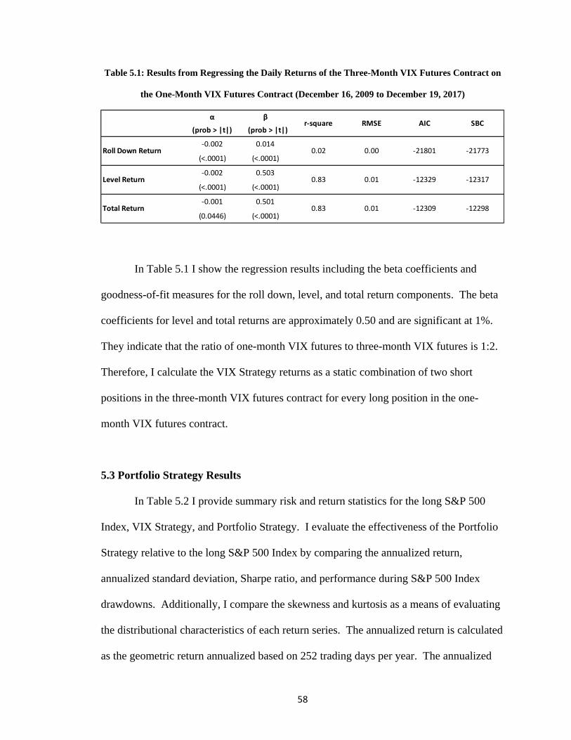
58
Table 5.1: Results from Regressing the Daily Returns of the Three-Month VIX Futures Contract on
the One-Month VIX Futures Contract (December 16, 2009 to December 19, 2017)
In Table 5.1 I show the regression results including the beta coefficients and
goodness-of-fit measures for the roll down, level, and total return components. The beta
coefficients for level and total returns are approximately 0.50 and are significant at 1%.
They indicate that the ratio of one-month VIX futures to three-month VIX futures is 1:2.
Therefore, I calculate the VIX Strategy returns as a static combination of two short
positions in the three-month VIX futures contract for every long position in the one-
month VIX futures contract.
5.3 Portfolio Strategy Results
In Table 5.2 I provide summary risk and return statistics for the long S&P 500
Index, VIX Strategy, and Portfolio Strategy. I evaluate the effectiveness of the Portfolio
Strategy relative to the long S&P 500 Index by comparing the annualized return,
annualized standard deviation, Sharpe ratio, and performance during S&P 500 Index
drawdowns. Additionally, I compare the skewness and kurtosis as a means of evaluating
the distributional characteristics of each return series. The annualized return is calculated
as the geometric return annualized based on 252 trading days per year. The annualized
α β
(prob > |t|) (prob > |t|)
-0.002 0.014
(<.0001) (<.0001)
-0.002 0.503
(<.0001) (<.0001)
-0.001 0.501
(0.0446) (<.0001)
r-square RMSE AIC SBC
Roll Down Return 0.02 0.00 -21801 -21773
Total Return 0.83 0.01 -12309 -12298
Level Return 0.83 0.01 -12329 -12317

59
standard deviation is calculated as the standard deviation of daily returns multiplied by
the square root of 252.
The returns presented in the S&P 500 Index Drawdowns section of Table 5.2 are
calculated as the cumulative compound returns during the period shown. The specific
dates were chosen based on the peak-to-trough decline for the S&P 500 Index.
Table 5.2: Risk and Return Statistics for the S&P 500 Index, VIX Strategy, and Portfolio Strategy
(December 16, 2009 to December 19, 2017)
The Portfolio Strategy outperforms the S&P 500 Index with approximately 28%
less standard deviation. The combination of a slightly better annualized return and lower
standard deviation results in the Portfolio Strategy having a higher Sharpe Ratio (1.1
versus 0.8) compared to the S&P 500 Index. Additionally, the skewness of the Portfolio
Strategy (-0.1) compared to the skewness of the S&P 500 Index (-0.4) indicates that the
Portfolio Strategy has less of a left tailed distribution compared to the S&P 500 Index.
S&P 500
Index
VIX
Strategy
Portfolio
Strategy
Annualized Return 11.7% 11.6% 11.8%
Annualized Standard Deviation 14.7% 12.4% 10.6%
Skewness -0.4 0.0 -0.1
Kurtosis 4.6 17.7 6.1
Sharpe Ratio 0.8 0.9 1.1
Means t -Test -0.3 0.4
F -Test 0.7 0.5
S&P 500 Index Drawdowns
May 2, 2011-Oct. 3, 2011 -19.4% 1.0% -7.6%
July 20, 2015-Aug. 25, 2015 -13.1% 1.9% -4.3%
Nov. 3, 2015-Feb. 11, 2016 -12.2% 0.2% -4.8%
60
The results for kurtosis show that the Portfolio Strategy has slightly more extreme
observations compared to the S&P 500 Index. However, the skewness results for the
VIX Strategy show that the extreme observations fall on both sides of the mean return.
During the periods identified as S&P 500 Index drawdowns, the Portfolio
Strategy greatly outperformed the S&P 500 Index. For example, during the period of
May 2, 2011-October 3, 2011 the S&P 500 Index declined 19.4% while the Portfolio
Strategy declined 7.6%. The outperformance during each drawdown period was a result
of the strong performance of the VIX and one-month VIX futures contract. For example,
the VIX increased in price from 16 to 45.45 from May 2, 2011 to October 3, 2011.
The Means t-Test values shown in Table 5.2 are the test statistics for comparing
the annualized returns of the Portfolio Strategy and VIX Strategy to the annualized
returns of the S&P 500 Index. The null hypothesis is equal annualized returns (i.e.,
𝐻0: 𝑟𝑝𝑜𝑟𝑡𝑓𝑜𝑙𝑖𝑜 𝑠𝑡𝑟𝑎𝑡𝑒𝑔𝑦 = 𝑟𝑆&𝑃 500 𝑎𝑛𝑑 𝑟𝑉𝐼𝑋 𝑠𝑡𝑟𝑎𝑡𝑒𝑔𝑦 = 𝑟𝑆&𝑃 500) against an alternative
hypothesis that they are not equal. The absolute critical value for a two-tailed test is 1.96.
The test statistics for the Portfolio Strategy (0.4) and VIX Strategy (-0.3) do not exceed
1.96 or -1.96 and therefore indicate that their annualized returns are not statistically
different from the annualized returns of the S&P 500 Index.
Table 5.2 includes the F-Test statistics for comparing the variances of the
Portfolio Strategy and VIX Strategy to the variance of the S&P 500 Index. The null
hypothesis is equal variances (i.e., 𝐻0: 𝜎𝑝𝑜𝑟𝑡𝑓𝑜𝑙𝑖𝑜 𝑠𝑡𝑟𝑎𝑡𝑒𝑔𝑦2 = 𝜎𝑆&𝑃 500
2 𝑎𝑛𝑑 𝜎𝑉𝐼𝑋 𝑠𝑡𝑟𝑎𝑡𝑒𝑔𝑦2 =
𝜎𝑆&𝑃 5002 ) against a two-tailed alternative hypothesis of unequal variances. The critical
value at the 0.01 significance level for a two-tailed F-Test is 1.000. The F-Test statistics

61
for both the Portfolio Strategy and VIX Strategy are less than 1.000 indicating that their
variances are statistically different from the variance of the S&P 500 Index.
The results shown in Table 2.3 and Table 5.2 compare to the results of Berkowitz
and DeLisle (2018) shown in Exhibit 5. Although the two analyses are conducted during
different dates and using different proportions of S&P 500 Index and VIX futures
contracts, the results from Table 2.3 and Table 5.2 can be used to compare against their
methodology and findings. For example, Berkowitz and DeLisle (2018) buy the new
month VIX futures contract only when the prior month-end VIX is below 20.2.
The results from Table 2.3 imply that Berkowitz and DeLisle (2018) should have
bought the new month VIX futures contract when the month-end VIX was equal to or
greater than 20.2. In Table 2.3 I show that the average total returns for the one-, three-,
and five-month VIX futures contracts are the greatest when VIX is equal to or greater
than 20.6 (fifth quintile). The results from Table 2.3 indicate that Berkowitz and DeLisle
(2018) could have produced more appealing results if they bought the new month VIX
futures contract when the prior month-end VIX was equal to or greater than 20.2.
The Portfolio Strategy results in Table 5.2 compare favorably to the results of
Berkowitz and DeLisle (2018) because of the VIX Strategy. The VIX Strategy mitigates
the negative roll down return of the one-month VIX futures contract by shorting three-
month VIX futures contracts while retaining an average positive level return. While they
don’t explicitly quantify the negative roll down returns of the VIX futures contracts, the
results from Table 2.4 show that the roll down component is accountable for the entire
negative total P&L (and return) of the one- and three-month VIX futures contracts.

62
Chapter VI
Summary and Conclusion
6.1 Summary of Findings
VIX futures began trading on the CBOE Futures Exchange in March 2004 and
have since provided a means of trading forward S&P 500 Index implied volatility. The
popularity of trading VIX futures contracts is measured by the increase in volume and
open interest of the one-month contract, which increased 500 times and 600 times,
respectively from March 2004 to June 2017. The VIX term structure is upward sloping
most of the time, although the realized volatility of the VIX term structure is inverted.
The performance of VIX futures contracts has garnered considerable attention in
the finance literature. However, most of the finance literature has focused on the total
returns with little attention directed at the decomposition of the returns. More
specifically, the finance literature has noted the negative performance of VIX futures
contracts but only a select number have tried to quantify how much of the negative return
is due to roll down. Therefore, my first research objective is to: determine what
proportion the roll down return represents of the negative total return to VIX futures
contracts.
I develop a methodology to decompose the total returns of VIX futures contracts
into the two return components, roll down and level. I find that roll down accounts for
most, if not all, of the negative returns for the one-, three-, and five-month VIX futures
contracts. Additionally, I derive the profit and loss (P&L) from roll down and level,
which is unique in the context of the existing finance literature.

63
The methodology extends to each point on the VIX futures term structure
allowing me to achieve the second research objective: to evaluate how returns, and
return components, vary across the VIX futures term structure. I present the time series
regressions I use to analyze the linear relationships between VIX and the return
components of the one-, three-, and five-month VIX futures contracts. Additionally, I
apply and discuss the principal component model to identify the latent factor structure of
the VIX term structure.
I discuss the results from my time series regression models. Specifically, I find
that the total return and level return beta coefficients decrease as the time to expiration
increases, which is indicative of an inverted realized volatility term structure. Using the
results of the principal component model, I find that level returns account for most of the
VIX futures variance.
I apply a Portfolio Strategy and compare the results to the return and risk
characteristics of the S&P 500 Index. The Portfolio Strategy is a combination of the VIX
Strategy and passive S&P 500 Index. The VIX Strategy is constructed using the time
series regression results. This analysis relates to my third objective: to evaluate whether
the regression results will allow me to construct a long-short VIX trading strategy using
one-month and three-month VIX futures contracts. I find that the Portfolio Strategy
outperforms the S&P 500 Index and has less risk.
6.2 Conclusions
These results indicate that the negative total return of the one- and three-month
VIX futures contracts is entirely due to the negative roll down returns. The negative roll

64
down return accounts for approximately 98.6% of the negative total return of the five-
month VIX futures contract. The results of the return and P&L decomposition for
multiple points on the VIX term structure are unique and add to the existing VIX term
structure literature. For example, the existing literature focuses on total return
calculations for the VIX futures contracts (Alexander and Korovilas (2013), Bekowitz
and DeLisle (2018), Simon and Campasano (2014), Whaley (2013)). Additionally,
literature showing P&L by roll down and level has not yet been identified.
Using these results, I conclude that the level return component is responsible for
more than 90% of the standard deviation of total returns for each VIX futures contract.
Additionally, the level return and total return standard deviations each decrease as the
time to expiration increases. These results are indicative of an inverted realized volatility
term structure and they are consistent with prior findings in the literature.
The Portfolio Strategy outperforms the S&P 500 Index with less risk. The
favorable results are attributable to the VIX Strategy. Specifically, the short three-month
VIX futures contracts offset the negative roll down of the one-month VIX futures
contract while the level return component of the one-month VIX futures contract
provides a hedge to a long position in the S&P 500 Index. These results highlight the
significance of disaggregating the total returns and P&L of the VIX futures contracts into
the components of roll down and level. Insight regarding the roll down and level
components from across the VIX term structure offer the ability to construct a strategy
that maximizes either component.

65
6.3 Future Areas of Research
The returns of the roll down and level return components vary greatly based on
the level of VIX. I find that the average roll down and level returns each increase as the
VIX level rises. Additionally, the standard deviation of the level return component
becomes greater as the VIX level increases. These results indicate that estimating the
time series regressions conditional on the VIX level would produce beta coefficient
estimates that materially change given different levels of VIX. For example, the
estimated beta coefficient of the level return component may become larger (smaller) for
higher (lower) levels of VIX. Additionally, the change in beta coefficient estimates for
different levels of VIX may not be linear, indicating that an element of convexity exists
in the return components.
A natural extension of this research is to conduct quantile regressions to estimate
the beta coefficients of the total return and return components (roll down and level) based
on quantile rankings of the VIX. The results from quantile regressions could be used to
conditionally adjust the ratio of one- and three-month VIX futures contracts used in the
VIX Strategy. A conditionally adjusted ratio should reduce the amount of under-hedge or
over-hedge during different market regimes.

66
References
Alexander, Carol and Dimitris Korovilas. “Volatility Exchange-Traded Notes: Curse or
Cure?” The Journal of Alternative Investments, Vol. 16, No. 2 (2013), pp. 52-70.
Anderson, T.W. and Raul P. Mentz. “On the Structure of the Likelihood Function of
Autoregressive and Moving Average Models.” The Journal of Time Series Analysis, Vol.
1, No. 2 (1980), pp. 83-94.
Berkowitz, Jason P. and R. Jared DeLisle. “Volatility as an Asset Class: Holding VIX in a
Portfolio.” The Journal of Alternative Investments, Vol. 21, No. 2 (2018), pp. 52-64.
Beutow, Gerald W. and Brian J. Henderson. “The VIX Futures Basis: Determinants and
Implications.” The Journal of Portfolio Management, Vol. 42, No. 2 (2016), pp. 119-130.
Brenner, Menachem, Jinghong Shu, and Jin E. Zhang. “The New Market For Volatility
Trading.” The Journal of Futures Markets, Vol. 30, No. 9 (2010), pp. 809-833.
Burghardt, Galen and Morton Lane. “How to tell if options are cheap.” The Journal of
Portfolio Management, Vol. 16, No. 2 (1990), pp. 72-78.
Byoun, Soku, Chuck C. Y. Kwok, and Hun Y. Park. “Expectations Hypothesis of the
Term Structure of Implied Volatility: Evidence from Foreign Currency and Stock Index
Options.” Journal of Financial Econometrics, Vol. 1, No. 1 (2003), pp. 126-151.
Campa, Jose Manuel, and P. H. Kevin Chang. “Testing the Expectations Hypothesis on
the Term Structure of Volatilities in Foreign Exchange Options.” The Journal of Finance,
Vol. 50, No. 2 (1995), pp. 529-547.
Carr, Peter and Liuren Wu. “Variance Risk Premiums.” The Review of Financial Studies,
Vol. 22, No. 3 (2009), pp. 1311-1341.
Cochrane, John H. and Monika Piazzesi. “Bond Risk Premia.” The American Economic
Review, Vol. 95, No. 1 (2005), pp. 138-160.
Cornell, Bradford. “Taking Stationarity Seriously.” The Journal of Portfolio
Management, Vol. 44, No. 3 (2018), pp. 1-4.
Coval, Joshua D., and Tyler Shumway. “Expected Option Returns.” The Journal of
Finance, Vol. 56, No. 3 (2001), pp. 983-1009.
Daigler, Robert T., Brice Dupoyet, Fernando M. Patterson. “The Implied Convexity of
VIX Futures.” The Journal of Derivatives, Vol. 23, No. 3 (2016), pp. 73-90.

67
Dew-Becker, Ian, Stefano Giglio, Anh Le and Marius Rodriquez. “The Price of Variance
Risk.” The Journal of Financial Economics, Vol. 123, No. 2 (2017), pp. 225-250.
Dotsis, George. “The Market Price of Risk of the Variance Term Structure.” Journal of
Banking and Finance, Vol. 84, (2017), pp. 41-52.
Enders, Walter. Applied Econometric Time Series. Wiley, Fourth Edition, (2015).
Eraker, Bjorn and Yue Wu. “Explaining the negative returns to volatility claims: An
equilibrium approach.” The Journal of Financial Economics, Vol. 125, No. 1 (2017), pp.
72-98.
Glasserman, Paul. “Forward and Future Implied Volatility.” The International Journal of
Theoretical and Applied Finance, Vol. 14, No. 3 (2001), pp. 407-432.
Hannan, E.J. “The Central Limit Theorem for Time Series Regression.” Stochastic
Processes and their Applications, Vol. 9, No. 3 (1979), pp. 281-289.
Heston, Steven L. “A Closed-Form Solution for Options with Stochastic Volatility with
Applications to Bond and Currency Options.” The Review of Financial Studies, Vol. 6,
No. 2 (1993), pp. 327-343.
Huang, Zhuo, Chen Tong, and Tianyi Wang. “VIX term structure and VIX futures
pricing with realized volatility.” The Journal of Futures Markets, Vol. 39, No. 1 (2019),
pp. 72-93.
Huskaj, Bujar and Marcus Nossman. “A term Structure Model for VIX Futures.” The
Journal of Futures Markets, Vol. 33, No. 5 (2013), pp. 421-442.
Johnson, Travis L. “Risk Premia and the VIX Term Structure.” The Journal of Financial
and Quantitative Analysis, Vol. 52, No. 6 (2017), pp. 2461-2490.
Lin, Yueh-Neng. “Pricing VIX Futures: Evidence from integrated physical and risk-
neutral probability measures.” The Journal of Futures Markets, Vol. 27, No. 12 (2007),
pp. 1175-1217.
Litterman, Robert and Jose Scheinkman. “Common Factors Affecting Bond Returns.”
The Journal of Fixed Income, Vol. 1, No. 1 (1991), pp. 54-61.
Lu, Zhongjin and Yingzi Zhu. “Volatility Components: The Term Structure Dynamics of
VIX Futures.” The Journal of Futures Markets, Vol. 30, No. 3 (2010), pp. 230-256.
Mixon, Scott. “The Implied Volatility Term Structure of Stock Index Options.” The
Journal of Empirical Finance, Vol. 14, No. 3 (2007), pp. 333-354.
Natenberg, Sheldon. Option Volatility & Pricing. McGraw-Hill Education, (2014).

68
Nossman, Marcus and Anders Wilhelmsson. “Is the VIX Futures Market Able to Predict
the VIX Index? A Test of the Expectations Hypothesis.” The Journal of Alternative
Investments, Vol. 12, No. 2 (2009), pp. 54-67.
Simon, David P. and Jim Campasano. “The VIX Futures Basis: Evidence and Trading
Strategies.” The Journal of Derivatives, Vol. 21, No. 3 (2014), pp. 54-69.
Tsay, Ruey S. Analysis of Financial Time Series. Wiley, Third Edition, (2010).
Whaley, Robert E. “Trading Volatility: At What Cost?” The Journal of Portfolio
Management, Vol. 40, No. 1 (2013), pp. 95-108.
Wooldridge, Jeffrey M. Introductory Econometrics A Modern Approach, South-Western
Cengage Learning, Fifth Edition, (2013).
Zhang, Jin E. and Yingzi Zhu. “VIX Futures.” The Journal of Futures Markets, Vol. 26,
No. 6 (2006), pp. 521-531.

69
Appendix A
VIX calculation
The VIX calculation is 𝜎2 =2
𝑇∑
∆𝐾𝑖
𝐾𝑖2 𝑒𝑅𝑇𝑄(𝐾𝑖) −
1
𝑇[
𝐹
𝐾0− 1]2 where 𝜎 =
𝑉𝐼𝑋
100, T is the time to
expiration where each calendar day is divided into minutes, F is the forward S&P 500 Index level
identified by the strike price where the absolute difference between call and put price is the
smallest, K0 is the at-the-money strike price and is the strike price that is immediately below F, Ki
is the ith out-of-the-money strike price for the calls and puts, ∆𝐾𝑖 =𝐾𝑖+1−𝐾𝑖−1
2 is the interval
between strike prices, R is the risk-free interest rate, and Q(Ki) is the midpoint of the bid-ask
spread for each option Ki.

70
Appendix B
Statistical Characteristics of VIX and VIX Futures
Table B.1: Statistical Characteristics of Daily Returns for VIX and VIX Futures Contracts (December 16, 2009 to December 19, 2017)ab
a The data in Table B.1 has been rounded. b The t-Value in Table B.1 is used to test the significance of the sample mean relative to zero at the significance level of 0.05. Specifically, 𝐻𝑜: �̅� = 0 against
𝐻𝑎: �̅� ≠ 0. The critical value for the one-sided test is equal to 1.645.

71
Table B.2: VIX Futures Cumulative P&L (December 16, 2009 to December 19, 2017)
VIX Futures Contract Roll Down Level Total
Two-Month -$122,322 $9,677 -$112,645
Four-Month -$67,014 -$5,426 -$72,440
Six-Month -$50,164 -$5,786 -$55,950
Quintile One (VIX: 9.1-12.7)
Two-Month -$27,715 -$20,005 -$47,720
Four-Month -$16,316 -$14,844 -$31,160
Six-Month -$11,553 -$13,137 -$24,690
Quintile Five (VIX: 20.6-48.0)
Two-Month -$7,686 $62,516 $54,830
Four-Month -$4,445 $49,845 $45,400
Six-Month -$4,620 $44,920 $40,300
Cumulative P&L

72
Appendix C
Partial Autocorrelations of VIX and VIX Futures Return
Figure C.1: Plot of the Partial Autocorrelations for the Daily VIX Return (December 16, 2009 to
December 19, 2017)

73
Figure C.2: Plot of the Partial Autocorrelations for the Daily One-Month VIX Futures Roll Down
Return (December 16, 2009 to December 19, 2017)
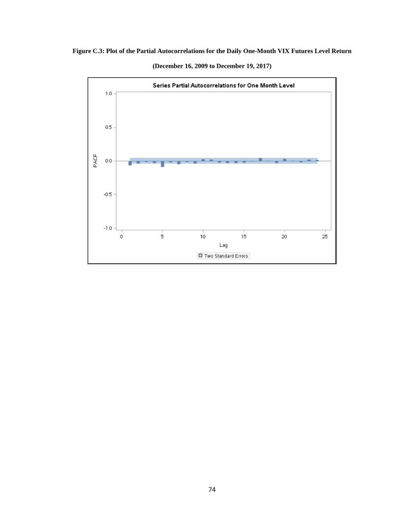
74
Figure C.3: Plot of the Partial Autocorrelations for the Daily One-Month VIX Futures Level Return
(December 16, 2009 to December 19, 2017)

75
Figure C.4: Plot of the Partial Autocorrelations for the Daily One-Month VIX Futures Total Return
(December 16, 2009 to December 19, 2017)

76
Appendix D
Return Correlation Matrix
Table D.1: Correlation Matrix Derived from Daily Returns (December 16, 2009 to December 19, 2017)
VIXOne Month
Roll Down
One Month
Level
One Month
Total
Three
Month Roll
Down
Three
Month
Level
Three
Month
Total
Five Month
Roll Down
Five Month
Level
Five Month
Total
VIX 1.00
One Month Roll Down -0.10 1.00
One Month Level 0.86 -0.12 1.00
One Month Total 0.83 0.13 0.97 1.00
Three Month Roll Down -0.09 0.36 -0.13 -0.04 1.00
Three Month Level 0.81 0.01 0.91 0.91 -0.05 1.00
Three Month Total 0.81 0.04 0.90 0.91 0.02 1.00 1.00
Five Month Roll Down -0.08 0.35 -0.12 -0.03 0.61 -0.05 -0.01 1.00
Five Month Level 0.78 0.00 0.87 0.86 -0.02 0.96 0.96 -0.05 1.00
Five Month Total 0.78 0.02 0.86 0.86 0.01 0.96 0.96 0.01 1.00 1.00
Pearson Correlation Coefficients


