doing justice to fundamentals in exchange rate forecasting

Doing Justice to Fundamentals in Exchange Rate

Forecasting: A Control over Estimation Risks

Biing-Shen Kuo∗

National Chengchi University

Taipei, Taiwan

Jan., 2007

Abstract

A shrinkage estimator that accounts for estimation risks is developed and employedto re-access whether the monetary fundamentals help predict changes in exchangerates. The suggested estimator is featured by optimally pooling information fromcross-sections across time and that from the individual time series of concern. Whilethe estimation risk in term of mean squared errors takes place in the presence of param-eter uncertainties, it is more problematic in the context of the exchange rate predictiveregression where the time series under study are typically short and the predictors arehighly persistent. Monte-Carlo simulations clearly demonstrate that comparing to theleast-square estimator, the magnitude of estimation errors associated with our shrink-age estimator is 10% to 35% less. Moreover, the risk reductions convert into sizablepower gains for tests for predictability, yielding a robust inference. In contrast to theprevious studies, a uniform evidence of the higher ability of monetary fundamentalsto forecast exchange rate movements is now found at both short and long horizons,whether in-sample or out-of-sample.

Keywords: random walk, fundamentals, exchange rate forecasting, shrinkage estimator,estimation risk, bootstrapJEL classification: C22, C52, C53, F31, F47

∗Correspondence: Department of International Business, National Chengchi University, Taipei 116, Tai-wan; Tel: (886 2) 2939 3091 ext. 81029, Fax: (886 2) 2937-9071, Email: [email protected]

1 Introduction

Whether economic fundamentals help predict exchange rate movements remains an unset-

tled issue. Messe and Rogoff in a series of papers in 80s first demonstrated that a simple

random walk forecast of the exchange rate outperforms alternative competing models based

on economic theories. This is to say that economic fundamentals such as money supplies,

interest rates and outputs simply contain little information in explaining future changes in

exchange rates, an evidence for the failure of the economic models. Some subsequent studies

do find success for fundamentals-related models that improve upon random walks out-of-

sample. Yet, the results do not lend enough credence to shaking the puzzling fact that the

exchange rates can be well-approximated as random walks, where their robustness remains

to be established. While it is still difficult to attribute fundamentals to changes in exchange

rates empirically, a recent theory of Engel and West (2004) justifies the near random-walk

behavior of the exchange rate, even in the presence of a link between exchange rates and

fundamentals.

Our study is motivated by one of the key assumptions on which the theory of Engel and

West is built: Fundamental variables have autoregressive unit roots. We take the assumption

as a natural beginning point of the study, and want to explore its empirical implications in

the predictive regressions used in the literature. In contrast to economic theory of Engel

and West, the paper attempts to offer econometric explanations to the near random-walk

exchange rates, and argues that previous empirical evidence for or against predictability in

exchange rate movements might have been considerably flawed by an existence of estimation

risk due to the strong persistence in fundamentals. The primary goal of the paper is in

a pursuit of a more reliable inference procedure for the predictability both in-sample and

out-of-sample by appropriately controlling for the estimation risk.

The persistence nature in fundamentals has created subtle problems for estimation of

and inference for the economic models. As one outstanding aspect of the problems, when

fundamentals are highly persistent, the OLS estimates are very likely to subject to small-

sample bias (Stambaugh, 1999). To correct for the bias, previous work appeals to the

bootstrap techniques (for example, Mark, 1995; Kilian, 1999). Although the bootstrap

helps reduce the bias, it introduces additional errors due to the bias estimation. On the

1

other hand, the persistence may lead to a substantial amount of variations in parameter

estimation in the region of near unit root, implying an efficiency loss (Phillips, 1998). As

a consequence of the loss, inferences for forecasting performance might well be biased in

favor of random walks, even when the data are generated by the fundamentals-based models

(Rossi, 2005). Nevertheless, it is well-known that there is a clear trade-off between bias and

estimation errors in small samples. Thus, much previous work just provides partial answers

to the predictability at issue by only looking at either bias or estimation errors. Little

existing work however investigates how the tradeoff would impact on model estimations and

forecasting inference.

The paper deals with both problems with small-sample bias and with estimation errors by

proposing a shrinkage estimator. The shrinkage estimator is derived by minimizing mean-

squared forecasting errors in the spirit of Judge and Mittelhammer (2004), and thus can

properly take into account the tradeoff. Specifically, the proposed estimator is an optimal-

weighted average of the OLS estimator from a certain exchange rate time series and the grand

average of the OLS estimators from the panel of the exchange rates series under study. In

this way, we exploit cross-sectional information as those using panel methods (Mark and

Sul, 2001), but in quite a different manner. By shrinking the asymptotically unbiased OLS

estimator full of estimation errors toward the biased grand average, the estimation risk can

now be considerably reduced. Of empirical significance is that the use of the shrinkage

estimator can potentially convert the estimation accuracy improvement into power gains for

the forecasting ability testing. As a result, when exchange rate variations is predictable,

the tests are ought to be more capable of detecting it, and the evidence by tests based

on the mounted estimator would tend to be more trustworthy than that presented before.

Our simulations clearly demonstrate the merits of the proposed semi-parametric estimator

in reducing the estimation risk. Calibrating parameters to the data set that Kilian (1999)

examined, our Monte-Carlo study shows that the power gains are found to be between 10%

and 30% greater than those using OLS estimates. A technical innovation of our approach lies

in an application of the bootstrap to parameter estimations, instead of plugging in consistent

estimates as suggested by Judge and Mittelhammer (2004).

Applying the newly developed estimator, we re-access the central issue of the study:

whether fundamentals can predict exchange rate movements. We also quantify potential

2

estimation risk which the previous research using conventional estimators could have been

subjected to. Significantly, we find that the fundamentals-based models now consistently

perform better than random walks, across various horizons. We conclude that the inability

of the economic models to yield better forecasts might well be due to the estimation risk

that has not been accounted for.

The remainder of the paper is organized as follows. Section 2 describes the monetary

models of exchange rate determination and the corresponding predictive regression. In Sec-

tion 3 we develop the shrinkage estimator used in the paper. Section 4 numerically analyzes

the statistical advantages of the shrinkage estimator over the conventional estimator. Section

5 re-examines the exchange rate predictability, and presents the empirical findings. Finally,

Section 6 concludes. Technical descriptions of the shrinkage estimator is left to the appendix.

2 A monetary model of exchange rates and its VAR

representation

We consider a standard long-run models of exchange rates where purchasing power parity

and uncovered interest parity are assumed to hold. Let eit be the log nominal exchange rate

at time t between currency i and the benchmark currency, denoted by ‘0’. The exchange

rate is currency i price of a unit of currency 0. Let rit be the nominal interest rate and pit

be the price level associated with currency i respectively. Thus,

rit − r0t = Eteit+1 − eit, (1)

eit = pit − p0t, (2)

where Et is the conditional expectation operator.

When money markets, both domestic and foreign, are in equilibrium,

mit − pit = λ yit − φ rit, (3)

m0t − p0t = λ y0t − φ r0t, (4)

where mit, yit and pit, respectively, are the log of money supply, output and price level

of currency i. The analogous variables for currency 0 are m0t, y0t, and p0t. Both money

equations share common income elasticity λ and interest semi-elasticity φ. Combining (1),

3

(2), (3) and (4),

Eteit+1 − eit = Et△eit+1 = −1

φ(fit − eit) = −1

φxit, (5)

where fit = (mit − m0t) − λ(yit − y0t) is the monetary fundamental values, and thus xit =

fit − eit is the deviation of the exchange rate from its fundamental value. The equivalence

relation simply states that the exchange rate is expected to react to deviations from its

fundamentals. The no bubble solution to the expectation difference equation (5) would

deliver the present value model:

eit =1

1 + φ

∞∑

j=0

(φ

1 + φ)jEtfit+j .

Deducting fit from both sides gives

eit − fit =

∞∑

j=1

(φ

1 + φ)jEt△fit+j .

These equations make it easy to explain a long-run equilibrium relation between exchange

rates and the monetary fundamentals. As long as fit is non-stationary processes, eit is an I(1)

process and fit − eit is an I(0) process by the aforementioned relation. As a result, there is a

cointegration between eit and fit with the pre-specified cointegrating vector (1,-1). Using the

VAR framework, the cointegration implies a bivariate vector error correction representation

for yit = (eit, fit)′: yit = c0 + c1yit−1 + · · ·+ cpyit−p +εit. Some re-arranging can yield another

vector error correction (VEC) model for eit and xit.1 In particular, our econometric analysis

centers on a VEC model that is frequently used in the exchange rate forecasting literature:

△eit = β(1)i xit−1 + ε1

it, (6)

△xit = αixit−1 +

pi∑

l=1

c2il△eit−1 +

pi∑

l=1

d2il△xit−1 + ε2

it, (7)

where (ε1it, ε2

it) are assumed to be i.i.d. with a vector mean zero and a nonsingular covariance

matrix. Equation (6) is the short-horizon predictive regression employed by Mark (1995),

Berkowitz and Giorgianni (1997), Groen (1997), Kilian (1997), Berben and Dijk (1998) and

Mark and Sul (2001) to study the exchange rate predictability. One of the goals of these

studies as well as ours is to investigate if the mean reversion of xit can improve the forecast

1This follows by noting that △xit = △fit −△eit.

4

accuracy by testing for β(1)i = 0 against β

(1)i > 0. The positive sign of the slope coefficient

β(i 1) suggests that eit is expected to decline when above its fundamentals. Both equation (6)

and (7) serve as data generating process in our bootstrapping algorithm after fitting them

to the data. Because the log exchange rate returns to its fundamental value over time, more

than 1-period ahead change in eit may be characterized by deviations from the monetary

fundamentals as well. Thus, the predictive regression (6) can in general be of the form:

eit − eit−k = β(k)i xit−k + εit, (8)

where k represents the forecast horizons and is set to 1, 4, 8, 12 and 16 in the analysis.

Not to complicate the use of notations, the superscript (k) will be saved from the exposition

following, unless there are confusions created.

Our analysis takes up two major related empirical concerns. As stated above, one would

be to search for the empirical validity for the monetary model of exchange rates using our

proposed estimator. By controlling for the estimation risk, the estimator is hoped to achieve

a high degree of statistical accuracy in establishing the proposition. Moreover, the previous

discussions suggest that for exchange rate to be predictable, exchange rates are ought to be

cointegrated with the monetary fundamentals first. Therefore, another task is to investigate

the existence of the cointegration between eit and fit based on the suggested estimator.

3 Econometric Framework

This section develops a shrinkage estimator that is to control potential estimation risks

associated with the predictive regression. The motivation for a need for the estimator will

be discussed immediately.

3.1 Sources of estimation risk

The OLS estimation of the slope coefficient tends to suffer more estimation risk than ordinary

regressions. It results from some distinctive characteristics for the predictive regressions.

First, the predictor xit, or the deviation of exchange rate from fundamentals, is documented

to be a highly persistently process. The high degree of persistence in forecasting variables,

however, may generate a biased estimate of βi in small samples, although do not alter the

unbiasedness asymptotically. The magnitude of the bias is positively proportional to the

5

degree of persistence in forecasting variables for a given sample size, as demonstrated by

Stambaugh (1999).

Second, the predictor possesses a much smaller variability than the dependent variable

does (Mark and Sul, 2004). It is regarded that the small variance might not affect some

statistical properties of the estimators asymptotically. But in finite samples, a small variance

in regressors suggests a small signal-to-noise ratio, yielding imprecise estimates of βi. It turns

out that the imprecision could not be safely ignored when taking into account another key

feature of predictive regressions as below.

Third, the dependent variable is long-horizon change in log exchange rate that amounts

to overlapping sums of short-horizon change in log exchange rates. Valkanov (2003) have

shown that in some parametric settings, the OLS estimator of βi might be inconsistent,

when the link of the small variance in predictors to the overlaps in dependent variables is

considered. In other words, the small-sample distributions of the estimates of βi is more

dispersed with the forecast horizon k. This is simply another reflection of the imprecise

estimation of βi due to the small variance.

The estimation risk appears to take a form of either bias or inefficiency, whether it is due

to the high persistence or the small variability. The little consensus emerging from empirical

findings in the literature may come from the fact that econometric methods adopted can only

deal with some parts of the risks. It is thus important to have a comprehensive approach

that is capable of controlling for the overall estimation risks. This will be the subject to be

studied in the next subsection.

3.2 A shrinkage estimator

To reduce the estimation risks in the context of predictive regressions, we consider a shrinkage

estimator for βi defined by

βi = ωi · βi + (1 − ωi) · β,

where ωi is the ‘shrinking factor’ that assigns weights to the two estimators in combination,

βi is the OLS estimator, and the grand average estimator is given by

β =

∑Ni=1 βi

N

6

which takes the average of all the OLS estimators of the slope coefficients of the N countries.

As it appears now, the shrinkage estimator considered is a Stein-like estimator which linearly

combines two alternative estimators that differ in their bias and precision characteristics.

Stein (1956) showed that shrinking sample means toward a fixed constant, under some

conditions, can reduce estimation risks. The key is to create a tradeoff between bias and

accuracy by introducing a biased estimator, represented by the fixed target, to combine with

the unbiased estimator, represented by the sample mean. The statistical decision theory

suggests the existence of an interior optimum in the tradeoff between bias and precision.

Taking a proper weighted average of the unbiased and the biased estimators would constitute

one of feasible approaches to attaining the optimal tradeoff. The idea of shrinkage has been

widely applied to the problem of portfolio selection (for example, Jorion, 1985; Dumas and

Jacquillat, 1990) and the context of prediction (Copas, 1983).

Our shrinkage estimator inherits the idea of Stein’s (1956) seminal work. To see this,

it is important to recognize that 1) the individual OLS estimator of the slope coefficient is

unbiased asymptotically, but has lots of estimation errors due to the small variance of and

high degree of persistence of the predictors, and that 2) the opposite is true for the grand

average of all the cross-sectional slope estimators which is subject to larger bias but less

estimation errors due to the averaging. Thus the intuition of the theory simply suggests that

taking a weighted average of the OLS estimator and the grand mean estimator is likely to

yield an estimator with less risk in the context of predictive regressions.

It is evident that the suggested estimator for the slope coefficients utilizes information

from cross-sections in a similar way that the panel-based estimators adopted by Groen (2000)

and Mark and Sul (2001) do. Like Stein, we are concerned with the estimation of several

unknown coefficients. It is natural that these Stein-like estimator makes best use of existing

information available. The implicit assumption underlying the use of information from cross-

sections for our estimator, however, is very much different from that for the panel-based

estimators. The panel-based estimators are built on the assumption that the slope coefficients

are all the same for all the cross-sectional countries. The panel approach to pooling the data

produces a single estimate. On the other hand, the shrinkage estimator allows for separate

slope estimate for each cross-section country as the OLS estimator does, but makes use of

the cross-sectional information that the OLS estimator does not. Thus both the shrinkage

7

estimator and the pooled estimator are the same to reduce the estimation errors, but differ

in the way how the cross-sectional information is processed. Yet, our shrinkage estimator has

the advantages of producing more reasonable slope estimates. When the truth is that the

slope coefficients are all the same across each cross-sectional countries, the difference between

the slope estimates from the two approaches should be insignificant, because by definition

the shrinakge estimator embraces the extreme situation. But if the slope parameters are all

different in each country, the panel approach by no means gives consistent slope estimate,

because of a false constraint imposed in estimation, while our shrinkage estimator still does,

as will be shown below.

The construction of the shrinkage estimator opens a few questions to be answered.

3.3 Shrinkage target

What is the rationale behind the choice of the grand average as the shrinkage target? The

grand average has been commonly employed in the literature. Lindley (1962) demonstrates

that the risk dominance of the Stein estimator when shrinking the sample mean toward the

grand mean estimator. Our choice reflects a belief that the slope coefficients is different and

near to each other. Like the constant target in the case of sample mean estimation, the grand

average plays the role of a restricted estimator, while the OLS estimator is the unrestricted

counterpart. Here the constraint imposed into our estimator is the slope coefficients of all

the country are the same. Conventional econometric wisdom would suggest that imposing

any structure or restriction in estimation brings forth efficiency gains, whether or not it is

true. Consequently, our shrinkage estimator performs best when each of the slope coefficients

coincides.

Alternative shrinkage targets as structures or constraints might exist. One shrinkage

target works well for a certain data set, but not necessarily for another. It is thus difficult

to tell which one works well a priori, without checking out-of-sample performance. This

study looks at a dataset of aggregate time series from major developed countries. Within

the circle, the transmission of shocks to fundamentals to exchange rates, if any, may vary

with the macro environment or the aggregate policy in each country, but at a similar speed.

The assumption of the slope heterogeneity is considered a reasonable one. We will show the

advantages of the chosen target through simulations.

8

3.4 Shrinking factor

Applications of the shrinkage estimator is not possible without knowing the shrinking factor

ωi. The subsection is devoted to how to determine and estimate it. The major goal for all

the existing estimators is in finite samples to minimize the estimation risk of the proposed

estimators. This entails a need to specify a loss function. We propose to use the quadratic

loss function. The loss function considers the tradeoff between bias and estimation errors

using a quadratic distance measure between the true and the estimated slope coefficient. It

gives rise to a risk function that calculates mean squared errors (MSE) as follows:

ℜ(βi, βi) = MSE(βi) = E[

(βi − βi)2]

.

Minimizing ℜ(βi, βi) with respect to ωi gives

ωi =MSE(β) − E

[

(βi − βi)(β − βi)]

MSE(βi) + MSE(β) − 2E[

(βi − βi)(β − βi)] .

We can describe the ‘optimal’ shrinking factor further, provided that the probability struc-

ture between the estimators is given. Without assuming normality, suppose the OLS esti-

mator and the grand average in finite samples is jointly distributed as:

[

βi

β

]

∼ P

[(

βi + γi,ls

βi + γi,g

)

,

(

σ2i,ls ρi

ρi σ2i,g

)]

,

where P can be any distribution function as long as the first and second moments exist and

are finite, and , and βi is the true value of the slope coefficient i. Note that γi,ls is the bias

associated with the OLS estimator due to the high degree of persistence in predictors, and

γi,g =P

i βi

N− βi, the distance of the true grand average from the true slope coefficient i.

Therefore, when the slope coefficients are all the same, γi,g = 0. A important feature from

the covariance matrix is to have the considered estimators correlated by an introduction of

ρi. The appearance of the correlation measure is unusual when understanding the shrinkage

estimator in an empirical Bayesian vein where it combines a prior, given by the grand

average estimate, with the sample information corresponding to the least squares estimate.

The typical empirical Bayesian approach assumes independence between prior and sample

information, regardless of whether the prior is estimated from the same dataset as the grand

average. Allowing for a correlation between the combined estimators may avoid damage in

9

estimations that takes place without considering the link.2 With some algebra calculations,3

ωi =1 −σi,ls + γ2

i,ls − ρi − γi,lsγi,g

σ2i,ls + γ2

i,ls + σ2i,g + γ2

i,g − 2ρi − 2γi,lsγi,g.

The expression offers some intuitions of how the weight is given to the combined estimators.

Higher weight is assigned to the grand average when the OLS estimator has a higher bias and

variance. But the estimator is drawn toward the OLS estimator in the case of high correlation

between the combined estimators. When there are increases in γi,g or σ2i,g, indications that

the true slope coefficients are so scattered not as the prior prescribes, the OLS estimator

receives more weight. This is because gains from information combination in both cases is

small. Thus, very importantly, the weight adapts itself to the data.

It is crucial both in theory and in applications to estimate the shrinking factor con-

sistently. A pre-requisite for establishing the consistency of the proposed estimator is the

weight consistency.4 Further, it controls the information quality represented by the com-

bined estimators. A correct inference from the data is very much dependent on a precisely

estimated weight. A technical innovation in this paper is to suggest a consistent bootstrap

procedure to estimate the weight parameter. The available estimator as suggested by Judge

and Mittelhammer (2004), though consistent, relies on the asymptotic argument, and its

finite-sample performance can be satisfactory only when the sample size is sufficiently large.

This might not be the case in the study because of a panel of short-spanned time series is

under investigation. Typically the bootstrap estimator have proven to display more robust

performance than the asymptotic counterpart. A more important justification for such a

bootstrap procedure is that no general consistent estimator has been mounted for the bias

parameters such as γit,l and γi,g. We appeal to the bootstrap procedure in order to render

our estimation and inference feasible in the subsequent empirical analysis. Very detailed

illustration of the bootstrap algorithm is given in the appendix to save the space.

2One more difference is that the Bayesian approach is in general not optimized with any particular lossfunction.

3A detailed derivation is given in the appendix.4We have shown in the appendix the consistency of the shrinkage estimator, given the existence of a

consistent estimator for the shrinking factor.

10

4 Risk reduction: simulation analysis

This section investigates to what extent the proposed estimator can improve over the tradi-

tional estimator in terms of risk reduction through simulations. To make our analysis more

realistic, the DGP calibrated to the actual data is considered. Further, to permit a direct

comparison, the data under simulation analysis now and empirical study later is the same

as that used in Kilian (1999).5 The data spans from 1973.I to 1997.IV, and contains the US

dollar exchange rates of the Canadian dollar, the German mark, the Japanese yen, and the

Swiss franc. Thus, the country number N = 4 in the study.

The DGPs are based on both the restricted VEC model under the null that the exchange

rate is unpredictable, and under the alternative that the fundamental helps to predict the

exchange rate, on the maintained assumption that the exchange rate and the fundamental are

cointegrated. The key difference in generating data under the null or the alternative thus lies

in whether βi is set to 0. The lag orders of △xit is determined using the Campbell-Perron’s

general-to-specific rule. A seemingly uncorrelated regression is then fit to the data after

the lag orders are settled. Each country is estimated a separate DGP, while the residuals

are allowed to be dependent cross-sectionally measured by the joint error covariance matrix

Σ. Vector sequence of the innovations are now drawn from N(0, Σ), where the covariance

matrix is estimated from the SUR residuals. The pseudo observations on △sit and △xit

are produced recursively based on the estimated version of (6) and (7). The MSEs under

the null and the alternative are computed and recorded individually using the artificial data

from 2000 replications.

Table (1) reports the relative empirical risks of the shrinkage estimator and the least-

square estimator under the null and the alternative processes, respectively. The important

and encouraging message coming out of the simulations is that the shrinkage estimator

empirically dominates the least-square estimator, regardless of which simulation scenario is

considered. But the dominance weakens slightly as the forecast horizon increases. Virtually

the risk reductions using the shrinkage estimator can be as large as between 10% and 35%.

A decomposition of the MSE clearly reveals that the risk reductions using the shrinkage

estimator attributes much more to the reductions in the estimation errors, implying accuracy

5All the data is available and can be downloaded from the homepage of Journal of Applied Econometrics.

11

gains. In some instances, the bias even increases due to use of the shrinkage estimator,

although the bias increases do not offset the error reductions.

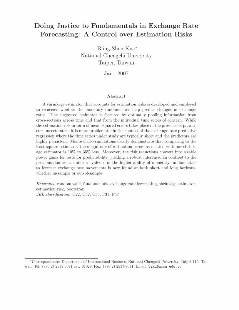
The risk improvements of the shrinkage estimator is embodied further into power gains in

testing. Table (2) presents the size-adjusted empirical power of using the shrinkage estimator

as the test statistic against the predictability alternative. An inspection of Table (2) shows

that the power gains from using the shrinkage estimator is 10% or more in many cases. For

Germany data, the power gain can be even up to 20%. An implication of the finding is merely

that the predictability alternative can now be better detected from the data when the test

statistics are based on the shrinkage estimator. Plot (1) depicts the clear difference between

the finite-sample distributions of the shrinkage estimator and the least-square estimator,

based on the Germany data. 6 In which, the distributions of the shrinkage estimator under

the null and the alternative are more centered. This is again due to the error reductions,

and exactly where power gains come.

5 A re-examination of the exchange rate predictability

We are in a position to re-examine the empirical validity of the exchange rate predictability

applying the shrinkage estimator. The testing strategy basically follows that utilized in Mark

(1995), Kilian (1999), and Mark and Sul (2001). These studies all base their inference on

the bootstrap approach in order to control for small-sample bias for which the asymptotic

approximation generally fails to correct. There are additional considerations for use of the

estimator. As discussed, the estimate for the optimal weight is given based on the bootstrap.

Next, the asymptotic theory for the proposed estimator has not been established yet. It is

expected that the asymptotic distributions of the statistics based on the shrinkage estimator

is ill approximated by the normal, because of the high degree of persistence characteristic in

predictors.

Before the asymptotic theory for the estimator is derived, inference on the predictability

here is mainly drawn from the bootstrap. The bootstrap conducted is very much the same as

described in the preceding simulation section, except the step about sampling innovations.

Instead of drawing samples from the parametric normal distribution, the re-samples are now

6Similar distribution patterns are also uncovered from other country’s data. They are not reported hereto economize the presentation.

12

drawn from a sequence of the restricted residual vectors. In other words, a non-parametric

bootstrap is employed. The restriction again is no exchange rate predictability, equivalently

βi = 0.

A by-product of the study is to test whether the exchange rate is cointegrated with

the fundamental, based on the shrinkage estimator. This can be done simply by imposing

another restriction that αi = 0 in (7) in the aforementioned re-sampling schemes.

5.1 A new look at cointegration

As has been emphasized, when the cointegration between the exchange rate and the funda-

mental does not come into existence, the exchange rate is simply unpredictable. We report

the results for testing for cointegration using the shrinkage estimator in Table (3).

The bootstrap coefficient test easily rejects the null of no cointegration between the

exchange rate and the fundamental, mostly at 5% significance level, with the exception of

Japan with k = 12. The testing results based on R2 lend additional credibility to the notion

of a cointegration between the exchange rate and the fundamental. Most of the corresponding

p-values for R2 are smaller than 5%, remarkably similar to those for the coefficient test.

Some obvious patterns on the estimated coefficients can be summarized from table. The

estimates for the slope coefficients are all shrunk further toward the grand average for all

the countries and all the forecast horizons (k). In general, the shrinkage estimates are less

dispersed than the OLS counterparts. This is to be expected from the shrinkage theorem. For

any particular country, the estimated slope coefficients increases as the horizons increases.

Nevertheless this should not be interpreted as an evidence for the increased long-horizon

predictability, as the cointegration can not be interchanged with the predictability in notions.

More importantly, the estimated slope coefficients for any fixed horizon are clearly seen to

vary to a certain degree. This appears to be consistent with our prior belief, but contradicts

the extreme assumption made in the panel-based approach that the slope coefficients are the

same for all the countries.

We now turn to the estimated optimal shrinking factors. The homogeneity in slope

coefficients would suggest that the estimated weights are similar in magnitude for any k. A

close inspection of the estimates shows however little evidence for the slope homogeneity. In

particular, some of the weights for Germany and Japan are negatively estimated. It is due to

13

that no constraint on the weight to be positive and smaller than one was placed in estimation.

Taking the normality approximation, if not too arbitrary, these negative weight estimates

are all covered in confidence intervals centered around the origin at 95% level, implying a

true weight indifferent from zero. In other words, the grand averages receives most of the

weight. Typically this might take place when the least square estimates are not reliable for

higher variance or larger bias. These are also the cases where the risk improvements over

the least square estimator may be substantial.

5.2 Out-of-sample forecast adjusted for risks

We access the relative forecast accuracy of the two competing models with DM (Diebold and

Mariano, 1995) statistic and Theil’s U statistic. It should be noted that the problem with

estimating the long-run variance precisely often leads to spurious inference, as documented

in the literature.

The forecast results are displayed in Tables (4) and (5). The former is based on the DM

statistic, and the latter the Theil’s U statistic. There is now stronger evidence presented for

the dominance of the monetary model over the random walk, after accounting for estimation

risks using the shrinkage estimates. With few exceptions, the p-values associated with the

shrinkage estimates for both statistics are smaller, relative to those associated with the least

square estimates.

It stands out from the results that controlling over the risks uncovers more favorable

evidence in supports of the monetary model, while there is essentially no evidence for so when

leaving the risks unattended. Instances of this are found more in Table (5) than in Table

(4). For example, at almost all horizons, the monetary model is found to be superior to the

random walk in terms of predictability for Germany and Japan. This contrasts sharply with

the previous findings where no predictability is reported. Considering the Theil’s U statistic

is more robust, this evidence lends quite a good deal of credence to the predictability at long-

horizon. Besides, there seems to have evidence of declining p-values as the prediction horizon

is increased, especially the results based on the Theil’s U statistic for all the countries but

Canada. Overall, by adjusting for the estimation risks, the evidence that the fundamentals

help forecast the exchange rate at short or even long horizon is stronger and clearer.

14

6 Conclusion

It is no denying that inference on the exchange rate predictability based on the univariate

predictive regression is not trustworthy due to estimation risks. The panel-based approach

exploiting cross-sectional information may reduce estimation errors, but incurs another type

of estimation risk with the extreme assumption of the parameter homogeneity. The shrink-

age approach proposed enjoys risk gains, while allowing for the parameter heterogeneity.

Our Monte-Carlo simulations further demonstrate that the merits of applying the shrink-

age approach converts into power gains in the testing context. Significant evidence for the

exchange rate predictability can now be found at least for short-horizons. Whether there

is evidence of higher predictability at longer horizons remains unconfirmed, although more

evidence points to be so after controlling over estimation risks.

One interesting question that deserves more research efforts is to investigate the effects of

the country number on the robustness of the inference. The shrinkage approach is basically

concerned with estimations of many unknown parameters. This is suggestive of further

risk improvements from utilizing more cross-sectional information. Rigorous research might

address to what degree an increase in country number can help reduce risks, and how much

economic value of additional risk reductions is worth.

Appendix 1: Derivation of the shrinking factor

The risk function as defined based on our shrinkage estimator can be expressed as

MSE(β(ωi)) = ω2i MSE(βi) + (1 − ωi)

2MSE(β) + 2ωi(1 − ωi)E[

(βi − βi)(β − βi)]

.

Minimizing it with respect to ωi gives the first-order condition as

2ωiMSE(βi) − (2 − 2ωi)MSE(β) + (2 − 4ωi)E[

(βi − βi)(β − βi)]

= 0,

from which the optimal shrinking factor can be found

ωi =MSE(β) − E

[

(βi − βi)(β − βi)]

MSE(βi) + MSE(β) − 2E[

(βi − βi)(β − βi)] .

15

as described. Note that

MSE(βi) = σ2i,ls + γ2

i,ls,

MSE(β) = σ2i,g + γ2

i,g,

E[

(βi − βi)(β − βi)]

= ρi + γi,lsγi,g.

Replacing with all the corresponding expressions above in the equation concerning the shrink-

ing factor then complete the derivation.

Moreover, it is easy to show that the optimal weight derived satisfies the second-order

condition, because

MSE(βi) + MSE(β) − 2 · E[

(βi − βi)(β − βi)]

= E[

(βi − β)2]

> 0.

In other words, βi is the minimum among all linear combinations of βi and β under the MSE

criterion.

Appendix 2: The consistency of the shrinkage estimator

We provide some regularity conditions under which the consistency can be established.

Suppose that T σ2i,ls

p→ σ2i,ls, T σ2

i,g

p→ σ2i,g, and T ρi

p→ ρi. Also assume that

γi,ls − γi,ls ≡ op(T−1), γi,g − γi,g ≡ Op(T

−1) and βi − βi ≡ Op(√

T−1

). Then, when σ2i,g 6= 0,

plim( ˜beta(ωi)) = plim[

ωiβi + (1 − ωi)β]

=plim(βi) + plim

[

ˆσi,ls2 + ˆγi,ls

2 − ρi − γi,lsγi,g

(βi − β)2· (βi − β)

]

=βi +Op(T

−1) + op(T−1) · op(T

−1) − Op(T−1) − op(T

−1) · Op(T−1)

Op(1) · Op(1)· Op(1)

=βi + op(1) = βi.

But if σ2i,g = 0, βi − βi ≡ Op(

√T

−1),

plim(β(ωi))

=plim(βi) + plim

[

T ˆσi,ls2 + T ˆγi,ls

2 − T ρi − T γi,lsγi,g

T (βi − β)2· (βi − β)

]

=βi +Op(1) + op(1) · op(T

−1) − Op(1) − op(1) · op(T−1)

Op(1) · Op(1)· op(1)

=βi + Op(1) · op(1) = βi.

16

This proves the consistency for the estimator.

Appendix 3: Bootstrap algorithm to estimating the optimal weight

The bootstrap procedures are to obtain robust estimates of the parameters appearing in the

optimal shrinking factor. The detailed illustrations are as follows:

1. Estimate △eit+k = βixit +εit+k and εi,t+k =∑m

l=1 ρilεi,t+k−l +vi,t+k with OLS, in which

the lag order m is chosen by the AIC criteria, and obtain βi, ρil, εi,t+k and vi,t+k.

2. Now draw from {vi,t+k} with replacements, and generate re-samples using the data-

generating process: △e∗it+k = βixit + ε∗it+k and ε∗i,t+k =∑m

l=1 ρilε∗

i,t+k−l + vi,t+k.

3. Regress △e∗it+k against xit with OLS and obtain the bootstrap estimates of the slope

coefficient, denoted by β∗

i .

4. Repeat steps 2 and 3 B0 times. Now compute the average bias byPB0

b=1βi−β∗

i,b

B0, and

deduct it from βi. This is the bootstrap bias-corrected estimate for the slope coefficient,

labeled asˆβi. Then the biased-corrected residuals can be computed accordingly by

ˆεit+k = △eit+k − ˆβixit.

5. Now generate the bootstrap samples based onˆβi, ˆεi,t+k, xi as if they are true ones by

repeating B0 times steps 2, 3, and 4. Thus, a sequence of { ˆβ∗

i } is generated. Repeat the

same procedures for different countries other than i, and obtain the bootstrap grand

average sequence of { ¯β∗} for the N countries.

Based on the two sequences of { ˆβ∗

i } and { ¯β∗} obtained from the aforementioned procedures,

the bootstrap estimate for the derived optimal shrinkage factor is computed as

ωi∗ =

∑

( ¯β∗ − ˆβi)

2 −∑

(ˆβ∗

i −ˆβi)(

¯β∗ − ˆβi)

∑

(ˆβ∗

i −ˆβi)2 +

∑

( ¯β∗ − ˆβi)2 − 2

∑

(ˆβ∗

i − ˆβi)(

¯β∗ − ˆβi)

.

References

[1] Berben, R.B. and D.J. van Dijk (1998), “Does the Absence of Cointegration Explain

the Typical Findings in Long Horizon Regressions,” Papers 9814/a, Erasmus University

of Rotterdam − Econometric Institute.

17

[2] Berkowitz, J. and L. Giorgianni (2001), “Long-Horizon Exchange Rate Predictability?”

Reviews of Economics and Statistics, 83(1), 81-91.

[3] Boswijk, H.P. (1994), ”Testing for an Unstable Root in Conditional and Structural Error

Correction Models,” Journal of Econometrics, 63(1), 37-60.

[4] Cheung, Y-W, M.D. Chin, and A. G. Pascual (2005), “Empirical Exchange Rate Models

of the Nineties: Are Any Fit to Survive?” Journal of International Money and Finance,

24, 1150−1175.

[5] Chinn, M.D. and R.A. Meese (1995), “Banking on Currency Forecasts: How Predictable

is Change in Money?” Journal of International Economics, 161−178.

[6] Diebold, F.X. and L. Kilian (2000), “Unit Root Tests are Useful for Selecting Forecasting

Models,” Journal of Business and Economic Statistics, 18, 265−273.

[7] Dumas, B. and B. Jacquillat (1990), “Performance of Currency Portfolios Chosen by a

Baysian Technique: 1967−1985,” Journal of Banking and Finance, 14, 539−558.

[8] Engel, C. and K.D. West (2005), “Exchange Rate and Fundamentals,” Journal of Po-

litical Economy, 113, 485−517.

[9] Engle, R.F., D.F. Hendry, and J.-F. Richard (1983), “Exogeneity,”, Econometrica, 51,

277−307.

[10] Efron, B. (1979), “Bootstrap Methods: Another Look at the Jackknife,” The Annals of

Statistics, 7(1), 1-26.

[11] Granger, C. W. J. and Newbold, P. (1974), “Spurious regressions in econometrics,”

Journal of Econometrics, 2, 111-120.

[12] Greene, W.H. (2000), Econometric Analysis, Prentice Hall, 4th Edition.

[13] Groen, J.J.J. (1999), “Long Horizon Predictability of Exchange Rates: Is it for Real?”

Empirical Economics, 24, 451−469.

[14] Groen, J.J.J. (2000),“The Monetary Exchange Rate Model as a Long-Run Phe-

nomenon,” Journal of International Economics, 52, 299−319.

18

[15] Hamilton, J.D. (1994), Time Series Analysis, Princeton University Press, Princeton,

NJ.

[16] Hansen, L.P. and R.J. Hodrick (1980), “Forward Exchange Rates as Optimal Predictors

of Future Spot Rates: An Econometric Analysis,” Journal of Political Economy, 88,

829−853.

[17] James, W. and C.M. Stein (1961), “Estimation with Quadratic Loss,” Proceedings of

the Fourth Berkeley Symposium on Mathematical Statistics and Probability (vol. 1),

Berkeley, California: University of California Press, 361−380.

[18] Jobson, J.D., B. Korkie and V. Ratti (1979),“Improved Estimation for Markowitz Port-

folios Using James-Stein Type Estimators,” Proceedings of the American Statistical As-

sociation, Business and Economics Statistics Section, 41, 279−284.

[19] Jorion, P. (1985), “International Portfolio Diversification with Estimation Risk,” Jour-

nal of Business, 58(3), 259−278.

[20] Jorion, P. (1986), “Bayes-Stein Estimation for Portfolio Analysis,” Journal of Financial

and Quantitative Analysis, 21, 279−291.

[21] Jorion, P. (1991), “Bayesian and CAPM Estimators of the Means: Implications for

Portfolio Selection,” Journal of Banking and Finance, 10, 717−727.

[22] Judge, G. G., W. E. Griffiths, R. C. Hill, and T.C. Lee (1980), The Theory and Practice

of Econometrics, New York: John Wiley & Sons.

[23] Judge, G.G. and M.E. Bock (1978), The Statistical Implications of Pre-Test and Stein-

Rule Estimators in Econometrics, Amsterdam: North−Holland.

[24] Judge G. G. and R. Mittelhammer (2004), “A Semiparametric Basis for Combing Esti-

mation Problems under Quadratic Loss,” Journal of American Statistical Association,

99, 479−487.

[25] Kendall, M.G. (1954), “Note on the Bias in the Estimation of Autocorrelation,”

Biometrika, 41, 403-404.

19

[26] Kilian L. (1999),“Exchange Rates and Monetary Fundamentals: What Do We Learn

from Long Horizon Regressions?” Journal of Applied Econometrics, 14, 491−510.

[27] Lindley, D.V. (1962), “Discussion of Professor Stein’s Paper,” Journal of the Royal

Statistical Society, Series B, 24, 285-288.

[28] MacKinnon, J.G. and Smith A.A. (1998), “Approximate Bias Correction in Economet-

rics,” Journal of Econometrics, 85, 205−230.

[29] Mark, N.C. (1995),“Exchange Rates and Fundamentals: Evidence on Long-Horizon

Predictability,” American Economic Review, 85, 201-218.

[30] Mark, N.C. and D. Sul (2001), “Nominal Exchange Rates and Monetary Fundamentals:

Evidence from a Seventeen Country Panel,” Journal of International Economics, 53,

29−52.

[31] Marriott, F.H.C. and J.A. Pope (1954), “Bias in the Estimation of Autocorrelations,”

Biometrika, 41, 393-402.

[32] Meese, R.A. and K. Rogoff (1983), “Emprircal Exchange Rate Models of the Seventies:

Do They Fit Out of Sample?” Journal of International Economics, 14, 3-74.

[33] Rossi, B. (2005), “Testing Long-Horizon Predictive Ability with High Persistence, and

the Meese-Rogoff Puzzle,” International Economic Review, 46, 61−92.

[34] Sclove, S.L., C. Morris, and R. Radhakrishman (1972), “Non Optimality of Preliminary

Test Estimators for the Multinormal Mean,” Annals of Mathematical Statistics, 43,

1481-1490.

[35] Stambaugh, R.F. (1999), “Predictive Regressions,” Journal of Financial Economics, 54,

375−421.

[36] Stein, C.M. (1955), “Inadmissibility of the Mean of a Multivariate Normal Distribu-

tion,” in Proceedings of the Third Berkeley Symposium on Mathematical Statistics and

Probability (vol. 1), Berkeley, California: University of California Press, 197−206.

[37] West, K.D. (1996), “Asymptotic Inference about Predictive Ability,” Econometrica,

64(5), 1067−1084.

20

[38] Zellner, A. and W. Vandaele (1974), “Bayes-Stein Estimators for k−Means, Regression

and Simultaneous Equation Models,” in S.E. Fienberg and A. Zellner, eds., Studies in

Bayesian Econometrics and Statistics in Honor of Leonard J. Savage, North−Holland,

Amsterdam, 627-653.

[39] Zviot, E. (1996), “The Power of Single Equation Tests for Cointegration when the Coin-

tegrating Vector is Prespecified,” Working paper, Department of Economics, University

of Washington.

21

-0.05 0.00 0.05 0.10 0.15

5

10

15

20

25

30OLS Stein

Null Alternative

Figure 1: The small-sample distributions of the shrinkage and OLS Estimators under H0

and Ha

22

Table 1: Relative estimation risk (Shrinkage/LS)

Country/Horizons 1 4 8 12 16H0

b Hac H0 Ha H0 Ha H0 Ha H0 Ha

MSE:a

Canada 0.829 0.830 0.817 0.822 0.801 0.836 0.817 0.857 0.848 0.865Germany 0.667 0.669 0.718 0.722 0.672 0.754 0.687 0.774 0.695 0.827Japan 0.621 0.624 0.701 0.774 0.655 0.809 0.682 0.840 0.706 0.861Switzerland 0.800 0.840 0.822 0.851 0.806 0.858 0.816 0.862 0.852 0.892

bias2:


variance:


a MSE is defined as the sum of the bias squared and the variance of the parameter estimates:

MSE(βi) = E[

(βi − βi)2

]

= E

{

[

(βi − E(βi)) + (E(βi) − βi)]2

}

= variance(βi) + bias(βi)2.

b The column gives the ratios of the MSE, bias squared, and variance of the Shrinkage estimates to by those of the

OLS counterparts, under the null of no predictability.c The column gives the ratios of the MSE, bias squared, and variance of the Shrinkage estimates to by those of the

OLS counterparts, under the alternative of predictability.

23

Table 2: Power performance of the shrinkage estimator

(a) 5% significance levelCountry/Horizons 1 4 8 12 16Canada 0.845a 0.850 0.854 0.792 0.723

(1.095)b (1.108) (1.131) (1.145) (1.172)Germany 0.616 0.680 0.607 0.540 0.507

(1.279) (1.444) (1.317) (1.239) (1.213)Japan 0.826 0.778 0.863 0.807 0.760

(1.309) (1.319) (1.214) (1.171) (1.193)Switzerland 0.735 0.715 0.757 0.720 0.628

(1.030) (1.033) (1.080) (1.136) (1.150)(b) 10% significance levelCountry/Horizons 1 4 8 12 16Canada 0.925 0.941 0.925 0.868 0.790

(1.085) (1.079) (1.087) (1.081) (1.078)Germany 0.802 0.783 0.804 0.770 0.713

(1.303) (1.288) (1.247) (1.207) (1.135)Japan 0.912 0.896 0.920 0.907 0.847

(1.078) (1.106) (1.108) (1.106) (1.107)Switzerland 0.896 0.849 0.867 0.818 0.754

(1.083) (1.060) (1.074) (1.068) (1.094)a The entries represent size-adjusted power of the Shrinkage estimator against the

alternative of exchange rate predictability.b The entries in parentheses represent the power performance of the Shrinkage

estimator relative to that of the OLS estimator (Shrinkage/OLS).

24

Table 3: Full-sample estimation results and tests for cointegration

statistics βia p-valueb R2 p-valuec βi β ωi std(ωi)

d

Canada:1 0.035 0.000 0.035 0.019 0.029 0.052 0.772 0.3114 0.131 0.000 0.104 0.010 0.106 0.207 0.734 0.2858 0.285 0.000 0.218 0.011 0.237 0.428 0.727 0.28912 0.370 0.011 0.194 0.031 0.230 0.625 0.742 0.31416 0.379 0.012 0.133 0.070 0.291 0.790 0.813 0.342

Germany:1 0.051 0.000 0.036 0.032 0.045 0.052 0.125 0.3404 0.195 0.021 0.119 0.004 0.178 0.207 0.183 0.2958 0.412 0.037 0.214 0.018 0.385 0.428 -0.035 0.28712 0.599 0.042 0.340 0.013 0.617 0.625 -0.047 0.32016 0.767 0.004 0.483 0.009 0.832 0.790 0.083 0.346

Japan:1 0.051 0.000 0.037 0.027 0.049 0.052 0.100 0.3284 0.199 0.042 0.121 0.006 0.207 0.207 0.008 0.3018 0.408 0.032 0.229 0.010 0.454 0.428 -0.067 0.31012 0.586 0.062 0.311 0.012 0.717 0.625 -0.111 0.32416 0.734 0.006 0.376 0.019 0.947 0.790 -0.145 0.347

Switzerland:1 0.072 0.000 0.064 0.000 0.087 0.052 0.578 0.3054 0.275 0.000 0.221 0.000 0.336 0.207 0.557 0.3218 0.542 0.000 0.366 0.001 0.634 0.428 0.589 0.30112 0.787 0.000 0.520 0.000 0.874 0.625 0.684 0.30516 1.048 0.001 0.722 0.000 1.090 0.790 0.874 0.320

a Shrinkage estimates is defined as βi = ωiβi + (1 − ωi)β, where βi is the OLS estimate of the slope

and the β is the grand average of the OLS estimates of the slopes of the 4 countries; ωi is the

estimated optimal weight.b,c P-value under the null of no exchange rate predictability (βi=0 and R2=0, respectively). Bold-

faced numbers refer to p-values less than 10%.d Standard deviation of the optimal weight estimates (ωi).

25

Table 4: Out-of-Sample forecast evaluations: DM Statistic

Country k DM(A)a p-value p-valueKc DM(20)b p-value p-valueKd

Canada 1 1.568 0.015 0.041 5.719 0.000 0.027

4 1.500 0.027 0.057 1.786 0.030 0.048

8 1.269 0.065 0.015 1.269 0.070 0.016

12 -0.518 0.333 0.064 -0.523 0.319 0.070

16 -1.378 0.655 0.110 -1.311 0.603 0.117maxe 1.568 0.052 0.060 5.719 0.005 0.056

Germany 1 0.534 0.095 0.151 0.841 0.093 0.1414 0.438 0.144 0.162 0.529 0.139 0.1608 0.433 0.169 0.218 0.433 0.180 0.21612 0.627 0.186 0.249 0.603 0.196 0.25016 0.796 0.191 0.321 0.777 0.195 0.314

max 0.796 0.288 0.273 0.841 0.300 0.268Japan 1 0.770 0.080 0.082 0.990 0.094 0.104

4 0.614 0.134 0.151 0.745 0.131 0.1448 0.855 0.129 0.133 0.890 0.136 0.13312 0.772 0.161 0.270 0.747 0.180 0.26916 0.729 0.170 0.451 0.717 0.180 0.433

max 0.855 0.283 0.240 0.990 0.280 0.253Germany 1 2.658 0.003 0.010 3.482 0.003 0.023

4 2.586 0.004 0.019 2.718 0.009 0.024

8 1.997 0.033 0.045 2.599 0.018 0.039

12 1.744 0.045 0.063 1.981 0.034 0.064

16 1.447 0.063 0.077 1.482 0.080 0.097

max 2.658 0.038 0.091 3.482 0.021 0.089

Notes: The DM statistic is defined as DM = d/q

2πfd(0)/Nf , where d = N−1

f

PTt=t0+k(u2

r,t −u2m,t) with ur,t and um,t

refer to the forecast errors of the random walk model and the monetary model, respectively. Nf is the number of recursive

forecasts, and t0 is the first date of forecast. fd(0) is the spectral density of (u2m,t − u2

r,t) evaluated at frequency 0. Its

consistent estimate fd(0) is obtained using Newey and West (1987).

a DM statistic computed with truncation lags under Bartlett window set to 20.b DM statistic with truncation lags under Bartlett window set by Andrews’s (1991) algorithm.c,d The corresponding p-value in Kilian (1999). Bold-faced numbers are those significant at 10% level.e Joint test statistic proposed by Mark (1995), taking the maximum of a sequence of DM statistics indexed by k.

26

Table 5: Out-of-sample forecast evaluations: Theil’s U

Country k Theil’s U p-value p-valueKa

Canada 1 0.971 0.009 0.042

4 0.936 0.030 0.068

8 0.900 0.043 0.057

12 1.063 0.549 0.094

16 1.179 0.761 0.151minb 0.900 0.081 0.137

Germany 1 0.989 0.061 0.1504 0.979 0.097 0.1698 0.961 0.109 0.21812 0.864 0.044 0.29116 0.729 0.010 0.473

min 0.729 0.013 0.283Japan 1 0.987 0.041 0.118

4 0.968 0.090 0.1578 0.927 0.069 0.14512 0.886 0.051 0.27416 0.838 0.045 0.534

min 0.838 0.053 0.250Swizerland 1 0.973 0.006 0.017

4 0.929 0.021 0.029

8 0.873 0.025 0.045

12 0.808 0.015 0.030

16 0.696 0.000 0.026

min 0.696 0.003 0.031

Notes: Theil’s U-statistic is defined as the ratio of the root-mean-square prediction

error of the monetary model based on the shrinkage estimator to that of the random

walk model. The null hypothesis is that the two models provide forecasts of equal

accuracy (U=1). The alternative hypothesis is that the monetary fundamentals is

more accurate (U<1).

a The corresponding p-values in Kilian (1999). Bold-faced numbers are those signif-

icant at 10% level.b Joint test statistic according to Mark (1995), which takes the minimun of a se-

quence of Theil’s U statistics indexed by k.

27

doing justice to fundamentals in exchange rate forecasting

Documents