2018 Nordic Conference on Development Economics

Helsinki, Finland

June 11-12, 2018

Does Relative Deprivation Induce Migration?

Evidence from Sub-Saharan Africa

Kashi Kafle, Rui Benfica, and Paul Winters

Research and Impact Assessment Division

IFAD, Rome, Italy

Motivation

• The traditional migration model (‘pull’ theory) considers wage or income

differentials between origin and destination as the primary cause of migration.

People migrate to maximize income or utility – welfare function approach (Harris and

Todaro 1970; Massey et al. 1993)

• The proponents of the ‘push’ theory of migration argue that social inequality

(relative deprivation) is one of the main causes of migration (Stark, 1984; Stark and

Taylor 1989, 1991)

• People migrate to minimize their feeling of deprivation relative to the community they

reside in- relative deprivation (RD) approach

• Some evidence on positive association between RD and migration (Quinn 2006;

Yitzhaki 1988; Stark and Taylor 1991)

• No conclusive evidence to support either approach (Flippen, 2013), the

longstanding ‘pull-push’ debate of migration is still unsettled.

Motivation

• Propensity to migrate is determined by both social inequality and absolute poverty

but it is expected to be higher in communities with higher social inequality (Stark

1984, stark and Yitzhaki 1988; Mehlum 2002; Czaika and de Haas 2012)

• While social inequality is believed to increase emigration, existing evidence

suggests that migration further increases inequality because migration led

economic growth is not broad-based (Barham and Boucher 1998; McKenzie and

Rapoport 2007; Czaika and de Haas 2012)

• Existing literature provides limited evidence on RD-Migration relationship, mostly

in the case of Mexico-US migration and the analysis is primarily based on relative

deprivation of income

• Examining RD-Migration in the SSA context is crucial because the region has

both persistent extreme poverty and a high degree of social inequality– factors that

fuel migration

Research Questions

• Does relative deprivation of consumption induce migration in sub-Saharan Africa?

• How does absolute consumption levels affect migration?

• Does relative deprivation of wealth have similar effects on migration?

• Does the RD-migration relationship persist over time and across countries?

Data

• First two waves of LSMS-ISA data from Tanzania, Ethiopia, Malawi, Nigeria,

Uganda

Wave 1 Wave 2 Attrition Panel

Country Year Sample Size Year Sample Size (%) Sample Size

Tanzania 2008/09 3265 2010/11 3168 2.9 3168

Ethiopia‡ 2011/12 3969 2013/14 3776 4.9 3776

Malawi 2010/11 3246 2013 3104 4.4 3104

Nigeria† 2010/11 4916 2012/13 4716 4.1 4437

Uganda† 2009/10 2975 2010/11 2716 8.7 2646

†In case of Uganda and Nigeria, the panel sample size is smaller than the wave 2 sample size because we lose observations to

measurement error. ‡All but Ethiopian sample is nationally representative.

Key Variables

• Outcome variable:

✓ Number of migrants in the household over the past 12 months

• Variables of interest:

✓ Monthly consumption per-adult equivalent (real dollars, local currency)

✓ Relative deprivation of consumption

✓ Wealth index (aggregated asset index)

✓ Relative deprivation of wealth

Key Variables

• Migration: Movement of individuals to any destination outside of the household

location for more than one continuous month in the last 12 months for

economic or other reasons, i.e., irrespective of the drivers of the movement.

• Relative Deprivation: Relative deprivation is an increasing function of not

having something one wants, sees someone else having, or sees as feasible to

have (Runciman, 1966).

✓ Hence a household’s relative deprivation depends on wellbeing status of other

households around it as well as the feeling of it’s members about their position

in the local wealth distribution.

Summary Statistics

Key variables Tanzania Ethiopia Malawi

Wave 1 Wave 2 Wave 1 Wave 2 Wave 1 Wave 2

Consumption (lcu) 56825.7 64622.7*** 538.9 451.2*** 14894.8 14621.8

(930.8) (1042.8) (10.3) (5.27) (295.7) (259.6)

Consumption (USD) [25.38] [28.86] [23.05] [19.3] [20.54] [20.16]

Consumption RD 0.30 0.31 0.34 0.30*** 0.30 0.31

(0.005) (0.005) (0.005) (0.005) (0.005) (0.005)

Wealth RD 0.73 0.79*** 0.65 0.61** 0.70 0.79***

(0.013) (0.014) (0.01) (0.01) (0.012) (0.013)

Number of migrants 0.45 0.63*** 0.28 0.28 0.18 0.38***

(0.016) (0.018) (0.012) (0.013) (0.01) (0.016)

Observations 3164 3164 3776 3776 3104 3104

Relative deprivation

• We follow Stark (1984) to calculate relative deprivation measure

• Relative Deprivation: 𝑅𝐷𝑖𝑟 𝑦 = 𝑦𝑟𝑖𝑦𝑟ℎ

1 − 𝐹 𝑥 𝑑𝑥

i: household

r: reference group (eg. enumeration area)

𝑦𝑟𝑖 is the value of consumption for household i,

𝑦𝑟ℎ is the highest value of consumption in the reference group r,

F(y): cumulative distribution of consumption y,

1-F(y): percentage of households with consumption higher than y,

• Similar approach for Relative deprivation of wealth

Empirical model

• Panel Fixed Effects:

𝑀𝑖𝑡 = 𝛼0 + 𝛼1𝑅𝐷𝑖𝑟𝑡 + 𝛽1𝐶𝑖𝑡 + θ𝑋 + 𝜇𝑖 + 𝑢𝑖𝑡

i, r, and t indicate a household, a reference group, and time, respectively

𝑀𝑖𝑡 is number of migrants

𝑅𝐷𝑖𝑟𝑡 is relative deprivation

𝐶𝑖𝑡 is logarithm of consumption expenditure.

𝑋 is a vector of control covariates,

𝜇𝑖 is fixed effects, and 𝑢𝑖𝑡 is idiosyncratic error.

• But, migration (𝑀𝑖𝑡) may be non-linear on consumption (𝐶𝑖𝑡), and endogenous

Is migration non-linear on consumption?

Methods: Empirical model

• Panel Fixed Effects: Quadratic (preferred model)

𝑀𝑖𝑡 = 𝛼0 + 𝛼1𝑅𝐷𝑖𝑟𝑡 + 𝛽1𝐶𝑖𝑡 + 𝛽2𝐶𝑖𝑡2 + θ𝑋 + 𝜇𝑖 + 𝑢𝑖𝑡

• Marginal effects of absolute consumption 𝛿𝑀𝑖𝑡

𝛿𝐶𝑖𝑡= 𝛽1 + 2. 𝐶𝑖𝑡 𝛽2

➢However, 𝛽1and 𝛽2 may be inconsistent because consumption is endogenous

i.e. 𝐸 𝑢 𝐶 ≠ 0

• We deal with endogeneity in two ways:

✓ IV: use multidimensional poverty index as IV for consumption

✓ Lagged regression: Regress 𝑀𝑖𝑡 in endline with baseline variables. Check

for consistency of results with main results

Results: Consumption space

LinearDependent Variable: Number of migrants

Tanzania Ethiopia Malawi Nigeria Uganda

Consumption RD 0.26* 0.24*** 0.11 0.26*** 0.45**

(0.14) (0.09) (0.10) (0.095) (0.18)

Log(Consumption) 0.35*** 0.030 0.068 0.06* 0.51***

(0.072) (0.043) (0.052) (0.034) (0.098)

Household size 0.15*** 0.054*** 0.11*** 0.16*** 0.77***

(0.018) (0.018) (0.014) (0.027) (0.034)

Dependency Ratio -0.013 -0.013** -0.015** 0.024*** -0.073***

(0.009) (0.005) (0.006) (0.007) (0.018)

Observations 6323 7288 6208 8780 5139

Other controls: Age, sex, and marital status of head, Rural and Ag. Household indicators

Results: Consumption space

QuadraticVariables Dependent Variable: Number of migrants,

Tanzania Ethiopia Malawi Nigeria Uganda

Consumption RD 0.46** 0.56*** 0.27** 0.36*** -0.20

(0.19) (0.11) (0.13) (0.10) (0.23)

Log(Consumption) 1.88* 1.49*** 1.35*** 0.97*** -3.51***

(1.05) (0.43) (0.51) (0.33) (0.93)

Log(Consumption) squared -0.067 -0.11*** -0.064** -0.049** 0.17***

(0.046) (0.032) (0.025) (0.018) (0.040)

Log(Cons.) + Log(Cons)2 =0

P-values 0.09 0.0005 0.008 0.003 0.0002

Marginal effects

25th percentile 0.495 0.286 0.187 0.136 0.017

50th percentile 0.443 0.199 0.132 0.088 0.187

75th percentile 0.381 0.107 0.072 0.038 0.368

95th percentile 0.273 -0.043 -0.039 -0.035 0.699

Observations 6323 7288 6208 8780 5139

Results: Demographic groupsConsumption space

Variables Rural Urban Female

headed

Male

headed

Fewer

youth

More

youth

Agricult

ural

Non-

agricultural

Tanzania:

Consumption RD 0.50* 0.31 0.31 0.72** 0.042 0.78** 0.68*** 0.031

(0.29) (0.36) (0.25) (0.34) (0.23) (0.33) (0.25) (0.37)

Log (Consumption) 1.98 2.81 0.96 4.42** 0.13 3.72** 2.50 1.83

(1.88) (1.80) (1.32) (1.89) (1.18) (1.68) (1.69) (1.69)

Ethiopia:

Consumption RD 0.59*** 0.82 0.35 0.68*** -0.21 0.93*** 0.59*** -0.088

(0.12) (0.87) (0.23) (0.13) (0.25) (0.16) (0.14) (0.36)

Log (Consumption) 1.68*** 1.44 1.10 1.61*** 0.17 2.15*** 1.48*** -0.10

(0.46) (2.51) (0.69) (0.52) (0.77) (0.64) (0.51) (1.18)

Malawi:

Consumption RD 0.50*** -0.32 0.39 0.22 0.17 0.10 0.27* 0.13

(0.14) (0.31) (0.26) (0.15) (0.18) (0.19) (0.15) (0.35)

Log (Consumption) 2.41*** -1.51 3.49*** 0.76 0.34 0.91 0.98 0.096

(0.70) (1.08) (1.15) (0.59) (0.70) (0.88) (0.66) (1.16)

RD increases migration

mostly in:

❑ Rural HHs

❑ Male headed HHs

❑ HHs with more youth

❑ Agricultural HHs

Results: Demographic groupsConsumption space

Variables Rural Urban Female

headed

Male

headed

Fewer

youth

More

youth

Agricul

tural

Non-

agricultural

Nigeria:

Consumption RD 0.33*** 0.55*** 1.13*** 0.23** -0.022 0.37** 0.49*** 0.073

(0.12) (0.21) (0.25) (0.11) (0.18) (0.15) (0.12) (0.24)

Log (Consumption) 0.85** 1.89*** 3.49*** 0.57 0.98** 0.62 1.32*** 0.98

(0.40) (0.73) (0.85) (0.37) (0.49) (0.50) (0.43) (0.60)

Uganda:

Consumption RD 0.094 1.18*** 0.074 0.48** 0.27 0.46 0.21 0.62***

(0.20) (0.45) (0.34) (0.21) (0.25) (0.28) (0.36) (0.23)

Log (Consumption) 0.27** 1.15*** 0.36** 0.51*** 0.27** 0.53*** 0.36* 0.57***

(0.11) (0.22) (0.18) (0.12) (0.13) (0.15) (0.20) (0.13)

RD increases migration

mostly in:

❑ Rural HHs

❑ Male headed HHs

❑ HHs with more youth

❑ Agricultural HHs

Results: Summary

• Results indicate that relative deprivation of consumption induces (increases)

migration, consistently so in multiple countries

• Absolute income (consumption) also increases migration but at a decreasing rate.

• People from households in the upper quartiles of consumption distribution are

less likely to migrate

• Relative deprivation of wealth also has positive association with migration

• The RD-Migration relationship does persist over time and across countries, in the

context of SSA.

• The positive effects of relative deprivation of consumption (and wealth) is mostly

concentrated in Rural, male headed, and agricultural households as well as

households with more youth

Conclusion

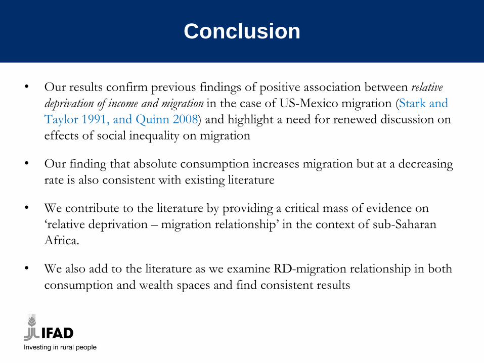
• Our results confirm previous findings of positive association between relative

deprivation of income and migration in the case of US-Mexico migration (Stark and

Taylor 1991, and Quinn 2008) and highlight a need for renewed discussion on

effects of social inequality on migration

• Our finding that absolute consumption increases migration but at a decreasing

rate is also consistent with existing literature

• We contribute to the literature by providing a critical mass of evidence on

‘relative deprivation – migration relationship’ in the context of sub-Saharan

Africa.

• We also add to the literature as we examine RD-migration relationship in both

consumption and wealth spaces and find consistent results

Implications

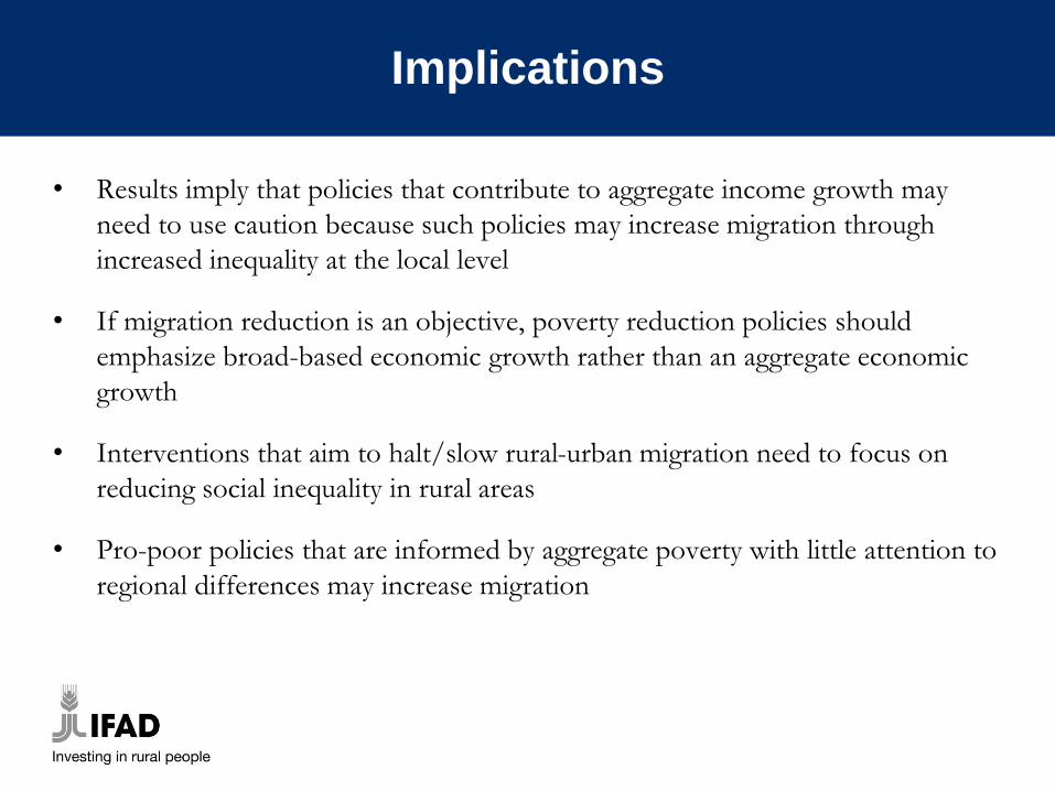
• Results imply that policies that contribute to aggregate income growth may

need to use caution because such policies may increase migration through

increased inequality at the local level

• If migration reduction is an objective, poverty reduction policies should

emphasize broad-based economic growth rather than an aggregate economic

growth

• Interventions that aim to halt/slow rural-urban migration need to focus on

reducing social inequality in rural areas

• Pro-poor policies that are informed by aggregate poverty with little attention to

regional differences may increase migration

THANK YOU!

Methods: Asset index

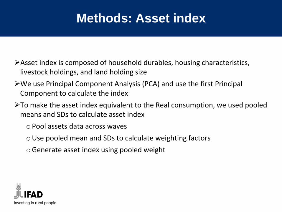
➢Asset index is composed of household durables, housing characteristics, livestock holdings, and land holding size

➢We use Principal Component Analysis (PCA) and use the first Principal Component to calculate the index

➢To make the asset index equivalent to the Real consumption, we used pooled means and SDs to calculate asset index

oPool assets data across waves

oUse pooled mean and SDs to calculate weighting factors

oGenerate asset index using pooled weight

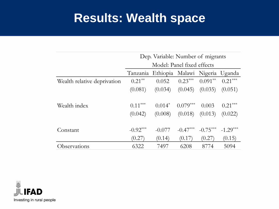
Results: Wealth space

Dep. Variable: Number of migrants

Model: Panel fixed effects

Tanzania Ethiopia Malawi Nigeria Uganda

Wealth relative deprivation 0.21** 0.052 0.23*** 0.091** 0.21***

(0.081) (0.034) (0.045) (0.035) (0.051)

Wealth index 0.11*** 0.014* 0.079*** 0.003 0.21***

(0.042) (0.008) (0.018) (0.013) (0.022)

Constant -0.92*** -0.077 -0.47*** -0.75*** -1.29***

(0.27) (0.14) (0.17) (0.27) (0.15)

Observations 6322 7497 6208 8774 5094

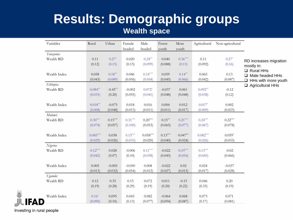
Results: Demographic groupsWealth space

Variables Rural Urban Female

headed

Male

headed

Fewer

youth

More

youth

Agricultural Non-agricultural

Tanzania:

Wealth RD 0.11 0.27* 0.020 0.24** 0.040 0.36*** 0.11 0.27*

(0.12) (0.15) (0.13) (0.099) (0.088) (0.13) (0.092) (0.16)

Wealth Index 0.058 0.18** 0.046 0.14*** 0.059 0.14** 0.065 0.13

(0.043) (0.089) (0.056) (0.054) (0.045) (0.066) (0.042) (0.087)

Ethiopia:

Wealth RD 0.084** -0.45** -0.002 0.072* -0.037 0.061 0.092** -0.12

(0.033) (0.20) (0.055) (0.041) (0.048) (0.048) (0.038) (0.12)

Wealth Index 0.018** -0.075 0.018 0.016 0.004 0.012 0.017* 0.002

(0.008) (0.048) (0.013) (0.011) (0.011) (0.017) (0.009) (0.023)

Malawi:

Wealth RD 0.30*** 0.15*** 0.31*** 0.20*** 0.15** 0.21*** 0.24*** 0.22***

(0.074) (0.057) (0.100) (0.053) (0.065) (0.077) (0.067) (0.078)

Wealth Index 0.085*** 0.038 0.15*** 0.058*** 0.13*** 0.047** 0.082*** 0.059*

(0.029) (0.026) (0.033) (0.020) (0.040) (0.024) (0.026) (0.033)

Nigeria:

Wealth RD 0.12*** 0.028 -0.006 0.11*** -0.022 0.19*** 0.13*** -0.02

(0.042) (0.07) (0.10) (0.038) (0.045) (0.054) (0.045) (0.066)

Wealth Index 0.005 -0.005 -0.050 0.008 -0.022 0.02 0.024 -0.037

(0.013) (0.032) (0.054) (0.012) (0.027) (0.015) (0.017) (0.028)

Uganda:

Wealth RD 0.12 0.35 0.15 0.072 0.011 -0.15 0.046 0.20

(0.19) (0.28) (0.29) (0.19) (0.20) (0.22) (0.33) (0.19)

Wealth Index 0.16* 0.095 0.043 0.082 -0.064 0.068 0.073 0.071

(0.090) (0.10) (0.13) (0.077) (0.094) (0.087) (0.17) (0.081)

RD increases migration

mostly in:

❑ Rural HHs

❑ Male headed HHs

❑ HHs with more youth

❑ Agricultural HHs

Summary statistics

Tanzania Ethiopia Malawi

Wave 1 Wave 2 Wave 1 Wave 2 Wave 1 Wave 2

Household characteristics

Household size 5.09 5.25** 5.13 5.78*** 4.79 5.24***

(0.050) (0.051) (0.037) (0.039) (0.040) (0.041)

Number of children, 0-14 2.34 2.34 2.43 2.41 2.29 2.45***

(0.034) (0.034) (0.028) (0.028) (0.029) (0.030)

Number of adults, 15-64 2.64 2.70 2.50 2.51 2.33 2.57***

(0.029) (0.029 (0.021) (0.021) (0.022) (0.024)

Dependency Ratio 1.65 1.70 1.56 1.97*** 1.79 1.68

(0.051) (0.053) (0.039) (0.044) (0.054) (0.048)

Rural residence (1=Yes, 0=No) 0.74 0.71*** 0.94 0.94 0.85 0.84

(0.008) (0.008) (0.004) (0.004) (0.006) (0.007)

Household head’s characteristics

Age 46.0 47.5*** 44.5 46.0*** 42.6 45.2***

(0.28) (0.27) (0.25) (0.25) (0.29) (0.28)

Sex (1=Female, 0= Male) 0.25 0.26 0.20 0.22 0.24 0.24

(0.008) (0.008) (0.006) (0.007) (0.008) (0.008)

Marital status (1= Married, 0=else) 0.73 0.72 0.81 0.78*** 0.76 0.76

(0.008) (0.008) (0.006) (0.007) (0.008) (0.008)

Key variables of interest

Consumption (local currency) 56825.7 64622.7*** 538.9 451.2*** 14894.8 14621.8

(930.8) (1042.8) (10.3) (5.27) (295.7) (259.6)

Consumption (US Dollars) [25.38] [28.86] [23.05] [19.3] [20.54] [20.16]

Consumption RD 0.30 0.31 0.34 0.30*** 0.30 0.31

(0.005) (0.005) (0.005) (0.005) (0.005) (0.005)

Wealth index -0.85 -0.81 -1.21 -1.03*** -0.55 -0.45*

(0.049) (0.051) (0.030) (0.023) (0.037) (0.041)

Wealth RD 0.73 0.79*** 0.65 0.61** 0.70 0.79***

(0.013) (0.014) (0.01) (0.01) (0.012) (0.013)

Household has migrants (1=Yes) 0.28 0.40*** 0.18 0.17 0.12 0.24***

(0.008) (0.009) (0.006) (0.006) (0.006) (0.008)

Number of migrants 0.45 0.63*** 0.28 0.28 0.18 0.38***

(0.016) (0.018) (0.012) (0.013) (0.01) (0.016)

Observations 3164 3164 3776 3776 3104 3104

Summary statistics

Nigeria Uganda

Wave 1 Wave 2 Wave 1 Wave 2

Household characteristics

Household size 5.89 6.42*** 5.90 6.42***

(0.047) (0.049) (0.069) (0.07)

Number of children, 0-14 2.47 2.58** 2.69 2.84**

(0.033) (0.034) (0.043) (0.042)

Number of adults, 15-64 2.93 3.29*** 2.75 2.87*

(0.027) (0.030) (0.035) (0.036)

Dependency Ratio 1.67 1.75 1.59 1.72

(0.042) (0.045) (0.051) (0.055)

Rural residence (1=Yes, 0=No) 0.70 0.70 0.78 0.84***

(0.007) (0.007) (0.008) (0.007)

Household head’s characteristics

Age 49.8 52.2*** 44.2 44.9

(0.23) (0.23) (0.31) (0.31)

Sex (1=Female, 0= Male) 0.15 0.15 0.28 0.31

(0.005) (0.005) (0.009) (0.009)

Marital status (1= Married, 0=else) 0.81 0.78*** 0.70 0.71

(0.006) (0.006) (0.009) (0.009)

Key variables of interest

Consumption (local currency) 8275.6 12262.2*** 76675.0 64842.3***

(105.7) (291.5) (2034.4) (1914.6)

Consumption (US Dollars) [22.9] [33.9] [21.30] [18.01]

Consumption RD 0.30 0.31** 0.35 0.38***

(0.005) (0.005) (0.006) (0.006)

Wealth index -0.01 -0.06 0.031 -0.047

(0.036) (0.035) (0.036) (0.036)

Wealth RD 0.68 0.68 0.70 0.69

(0.011) (0.011) (0.012) (0.011)

Household has migrants (1=Yes) 0.18 0.30*** 0.51 0.59***

(0.006) (0.007) (0.01) (0.009)

Number of migrants 0.33 0.58*** 1.13 1.53***

(0.014) (0.018) (0.032) (0.040)

Observations 4437 4437 2576 2576

Motivation

➢Migration, both international and domestic, is one of the major policy concerns in the world

➢So is the case in sub-Saharan Africa:

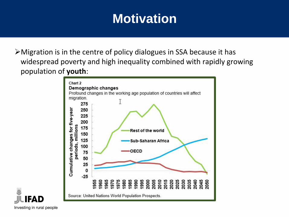
Motivation

➢Migration is in the centre of policy dialogues in SSA because it has widespread poverty and high inequality combined with rapidly growing population of youth: