does foreign innovation affect domestic wage inequality?

Journal of International Economics 47 (1999) 61–89

Does foreign innovation affect domestic wage inequality?a , b*Alison Butler , Michael Dueker

aDepartment of Economics, Florida International University, University Park, Miami, FL 33199,USA

bResearch Department, Federal Reserve Bank of St. Louis, P.O. Box 442, St. Louis, MO 63166,USA

Received 17 March 1996; accepted 23 December 1997

Abstract

We use an open-economy product-cycle model of domestic high-tech / low-tech wages tomotivate an empirical specification and test key model-implied restrictions. With data for 11countries from an internationally comparable data set from the OECD, we conduct panelcointegration analysis that supports the hypothesis that foreign and domestic innovationrates affect domestic wage inequality by equal and opposite magnitudes. The estimatedelasticities imply that a 10% increase in the domestic (foreign) innovation rate leads to a 3%increase (decrease) in the high-tech wage rate, relative to the low-tech wage. An atheoreticempirical regression that includes several of the same variables, but not the samespecification as the product-cycle model, fails to yield significant results, in contrast to thespecification derived from the product-cycle model. 1999 Elsevier Science B.V. Allrights reserved.

Keywords: Innovation; Wage differentials; Foreign competition; Patents

JEL classification: F41; J31; C23

1. Introduction

As international competition in high-technology goods increases and skillspremia widen within countries, the question arises: Is there any relationshipbetween the relative pace of innovation worldwide and changes in domestic wageinequality? Aspects of this issue have been examined in several diverse literatures.

*Corresponding author. Tel.: 11 305 3482682; fax: 11 305 3481524; e-mail: [email protected]

0022-1996/99/$ – see front matter 1999 Elsevier Science B.V. All rights reserved.PI I : S0022-1996( 98 )00014-2

62 A. Butler, M. Dueker / Journal of International Economics 47 (1999) 61 –89

Recent theoretical work in international trade has examined the reciprocalimplications of technological change and international trade, especially howinnovation affects the terms of trade, cross-country wage differentials and

1economic growth. These models, however, do not address the possible domesticredistributive effects of foreign innovation, because the models assume only onetype of worker in each country. Empirical work views the wage differential fromtwo related perspectives. One approach is to examine the effects of trade on wage

2inequalities. The other approach is to examine domestic reasons for changes in3wage inequality, particularly in the 1980s. While the latter research acknowledges

the key role technology may play, only Mincer (1991) includes a measure of4domestic innovative activity. Separately, these individual strands of research are

unable to address the public debate regarding the role of international competitionin new technologies on domestic wage differentials.

The work presented here attempts to bridge these divergent strands of researchby presenting a general equilibrium product-cycle model and using it as the basisfor an empirical examination of domestic high-technology/ low-technology wagesin countries. We use Butler’s (1997) open-economy product-cycle model, whichincludes two sectors in each country: An innovating (high-technology) sector andnoninnovating (low-technology) sector. Two types of workers populate theeconomy, with the more skilled workers employed in the innovating sector and the

5lower-skilled workers in the noninnovating sector. Once the production technolo-gy of a good becomes internationally available through technology transfer orpatent expiration, that variety is produced in the low-technology sector, where

6perfect competition holds and labor is cheaper. Because both countries have anoninnovating sector, production of a new variety is eventually transferred fromthe innovating sector of one country to the noninnovating sector of both countries.

This product-cycle model implies that the relative wage between workers inhigh- and low-technology industries within a country (hereafter called thedomestic relative wage) is a function of not only of the rate of domesticinnovation, but of foreign innovation as well. In particular, assuming free trade

1See, for example, Grossman and Helpman (1991b) and Stafford and Johnson (1993).2This literature has primarily focused on the U.S. economy. See the surveys by Burtless (1995) and

Kosters (1994) and the sources therein.3See, for example, Katz and Murphy (1992); Mincer (1991) for the United States and OECD (1993),

and Davis (1992) for European countries.4Berman et al. (1994) include R & D spending in their estimation, but they focus on labor demand

rather than wages.5We assume that the workers in the high-technology industries are higher skilled than those

employed in the low-technology sector. We find empirical support for this assumption, given thataverage wages are higher for workers in the high-technology sector for all countries and all years, forall three relative wage classifications.

6The model also examines what happens if the wage differential is less than one, that is, iflow-skilled workers are no longer cheaper than skilled workers. However, in the data set used, workersin the high-technology sector receive a higher wage for all countries across all years.

A. Butler, M. Dueker / Journal of International Economics 47 (1999) 61 –89 63

with immobile labor, the model implies that equivalent changes in the rate offoreign and domestic innovation affect the relative wage by equal (and opposite)magnitudes; the domestic relative wage depends on the worldwide supply ofhigh-tech workers, where foreign high-tech workers are weighted by their relativeinnovation rates.

To test for the impact that foreign and domestic innovation rates have on thedomestic relative wages, we use data for eleven industrial countries spanning theyears 1971–1992. The data are from an internationally comparable data setcompiled by the OECD that has consistent industrial classifications for manufac-turing wage and employment data. The model is estimated using modern panelcointegration methods that allow for heterogeneous cross-country dynamics andendogenous regressors. The theoretical model does not allow for technologytransfer across high-technology industries and so abstracts from the possiblespillover effect of innovation in one country on innovation in another. However,our measure of innovative activity will increase if an increase in innovation in onecountry leads to an increase in innovative activity in another, although the possibleinteraction is not included in the model.

The product-cycle model carries strong implications for domestic relative wagesby giving equal importance to foreign and domestic efficiencies in developing newproducts. This proposition finds strong support in the data. Although not all of therestrictions implied by the product-cycle model hold, the product-cycle modelsignificantly outperforms an atheoretic specification.

The next section presents Butler’s (1997) general-equilibrium, product-cyclemodel. The subsequent section contains a description of the data and highlights thehypotheses concerning foreign and domestic innovation rates. The econometricmethods and results follow. The paper concludes with a summary of the findings.

2. The model

2.1. The household sector

Consumers have identical time-separable preferences, characterized by astandard intertemporal utility function. Consumers value both variety and quantity,as represented by the following instantaneous constant elasticity of substitution(CES) utility function:

N 1 /ut

uu 5 E C(a) da 0 ,u , 1 (1)t 3 4a50

where: C(a)5consumption of variety a and u 5weight consumers place onquantity relative to variety.


Following Grossman and Helpman (1991a), we represent, without any loss ofgenerality, the set of brands available on the market by the interval [0, N(t)]. Withthis convention, the length N(t) represents the span of products invented beforetime t. To simplify notation, we refer to length N as the numerical ‘‘measure’’ or‘‘range’’ of available varieties.

To avoid the problem of diverging to an infinite range of available varieties,some varieties are assumed to go out of fashion and are no longer consumed (or

7produced) . The number of varieties that goes out of fashion is given at any timeby gN(t), where g is the parameter determining the rate at which varieties go out

8of fashion, g.0. Because preferences are the same in both countries, g is notcountry-dependent. Utility is maximized at each moment of time, given theamount of variety available. Consumer goods are produced in three sectors: The

9innovating sectors in the two countries and in the low-technology sector. Weassume the input and output markets for varieties produced in the low-tech sectorare characterized by perfect competition and that production technology in thelow-technology sector is the same in both countries. These assumptions, alongwith symmetric preferences, ensures the prices of low-tech goods are the sameacross varieties. Choosing low-tech varieties as a numeraire, normalizing on theprice of low-tech varieties, denoting relative prices and wages by upper-case lettersand solving results in the following demand functions:

Ca 5 Y /Z for any variety a produced by the low technology sector. (2)la

2´C 5 P Y /Z for any variety a produced by the highla 1a

2 technology sector in Country 1. (3)

2´C 5 P Y /Z for any variety a produced by the high2a 2a

2 technology sector in Country 2. (4)

N(t ) 12´where: Z5e P da, for any good a; P denotes the price of variety a0 a ja

7This assumption ensures there is not an infinite amount of variety in the model. Most models usingthis specification of utility allow infinite growth in variety, which we think is unrealistic, particularlyfor empirical work. For a closed-economy model where the rate at which goods go out of fashion isendogenous, see Young (1993). Not every variety ceases to be consumed, as not all types of varietiesgo out of fashion. Rather, some proportion of varieties stops being consumed. Another approach wouldbe to have quality cycles, where innovation takes the form of improvements in existing products.Quality cycles are generated using Cobb–Douglas utility, in which there can be no demand foruninvented products (see, for example, Grossman and Helpman, 1991a,b).

8To simplify the analysis, we assume an equal proportion of varieties goes out of fashion in eachsector.

9Because the variety available in the low-technology sector is the same in both countries, the countrysubscript is suppressed.


produced by the innovating sector of Country j; ´51/(12u ) is the (constant)elasticity of substitution between any two varieties, and Y5world income.

2.2. Worker types

There are two types of workers in each country: low-productivity workers, whocan only work in the low-technology sector, and high-productivity workers, whocan work in either the high- or low-technology sector. Within the high-tech sector,high-skilled workers can be assigned (at the same wage rate) to innovative activityor production of high-tech goods for which the technology has not yet diffused tothe low-tech sector. Returns to skill are assumed to be zero in the low-tech sector,so that if skilled workers are employed in that sector, they receive the same wage

10as low-productivity workers in the low-technology sector. Workers are immobileinternationally. High-productivity workers are assumed to be homogeneous withina country, but have varying productivity across countries. Because labor is theonly input, cross-country differences in the high-tech wage are due solely tocross-country productivity differences and not factor proportions. The labor marketis perfectly competitive and wages are flexible. The reservation wage is assumedto be sufficiently below the wage in the low-technology sector to ensure allworkers are employed.

2.3. High-technology firms

All firms within a sector have identical innovation and production functions, buthigh-tech firms cannot produce varieties invented through the innovative activityof another firm, because the technology is assumed to be nontransferable until itdiffuses to the low-tech sector. Innovating firms, therefore, are product monopol-ists in the sense that they innovate goods that only they can produce, but free entryin innovation and consumers’ perfect substitutability among different varietiesensure zero economic profits in the long run. R & D is required for innovation tooccur and any given variety is produced by a single firm, although each firm canproduce more than one variety. Because technology is linear, the number and scale

11of firms are indeterminate. Technology transfer is assumed to be costless and thenumber of varieties transferred per unit of time is a fixed proportion of the numberof varieties available in the high-tech sector. Once a technology is transferred, it isonly produced in the low-tech sector due to lower labor costs. The structure of the

10There is no mechanism for workers to invest in acquiring skills.11We assume the number of firms is large enough that there is no strategic behavior between firms,

either in a country or across countries. While adding strategic behavior would be interesting, it wouldgreatly complicate the model and alter the focus of the paper.


innovating sector is the same in both countries. All results are derived for Country121. Results for Country 2 can be found by changing country-specific parameters.

The innovating firm solves for the optimal time path of variety by maximizingtotal discounted profits, given the price and output level for each variety, whichcome out of a static maximization problem. The amount of R & D labor the firmhires determines the breadth of varieties it produces. High-tech firms always havean incentive to innovate because they are continually losing varieties, due totechnology transfer and varieties going out of fashion. Because the innovation andproduction functions are linear with respect to the decision variables, the problemis solved for a representative firm and then aggregated. The problem is solvedrecursively: The production choice, subject to the demand function, is a staticproblem and solved first; the choice of R & D investment, and therefore theamount of variety, is dynamic and thus solved second.

Production of any variety is characterized by constant returns to scale, and givenby:

PQ 5 a L , for any single good a produced in the innovating sector, (5)1a 1 1a

a 5the productivity parameter associated with production workers in the innovat-1Ping sector of Country 1 and L 5the number of high-tech workers employed in1a

the production of single variety a in the innovating sector of Country 1.Demand is given by Eq. (3). The firm maximizes the profit function subject to

the production and demand constraints. The solution to the static maximizationproblem is given by:

2´Q 5 P Y /Z (6)1a 1a

P 5 W /(a u ) (7)1a 1 1

where W is the wage paid to workers in the high-tech sector. Because the1

right-hand side variables in Eq. (7) do not change as a changes, the price for allvarieties in this sector is the same, a markup over the wage. High-tech wages varyacross countries, however, so high-tech varieties produced in different countriesare sold at different prices. Eqs. (6) and (7) define the monopolist’s price andquantity produced of each high-tech variety as a function of economy-widevariables, and we denote these solutions as P and Q .1 1

Let firms be indexed such that N represents the range of varieties produced by1j

firm j. Then the law of motion that determines the firm’s contribution to variety inthe innovating sector of Country 1, which is the same for all firms, is given by:

RdN /dt 5 i L 2 k N 2 gN , 0 , i , 0 , k , 1 (8)1j 1 1j 1 1j 1j 1 1

12The productivities of R & D and production workers in the high-technology sector of two countriesare allowed to differ. In addition, no assumptions are made regarding the relative size of the laborforces in the two countries.


Rwhere: N (0)50; L is the number of R & D workers in firm j; i is the1j 1j 1

productivity parameter associated with R & D workers in Country 1; and k is the1

rate of technology transfer for Country 1.The problem facing firm j is to maximize expected discounted profits, subject to

the innovation and production functions, the demand function, and the constraintthat R & D workers are required for innovation (that is, in the initial period thereare no high-tech varieties). Formally, firm j maximizes the following:

`2rt P P Rmax E e [P Q N 2 W (L 1 L )] dt, (9)1 1a 1j 1 1j 1j

R 0L 1j

Rsubject to (8), 0#L #L , L 5total high-technology labor in Country 1, and1j 1h 1h

r5producers’ discount rate, which is assumed to be the same for both countriesand equals the consumer’s discount rate.

Eq. (9) shows that the firm’s intertemporal decision concerns how muchresearch to conduct to produce the optimal number of varieties through time.Because of the linear nature of the differential equation in Eq. (8), the solution issingular. A singular solution is the unique interior solution, where the presentdiscounted value of future profits exactly equals the cost of R & D. If the initialconditions are such that the value of R & D workers is not consistent with thesingular solution for variety, there are two possible outcomes. If the cost of R & Dis low relative to future discounted profits, workers will be employed in R & Duntil the optimal level of variety is reached, at which point workers in that countrywill be allocated according to the singular solution. If the cost of R & D is toohigh relative to the future discounted profits there will be no innovating sector in

13that country (the optimal choice of R & D workers is zero).We cannot solve for the optimal number of R & D workers any one firm would

hire, because with linear technology the scale and number of firms is indetermi-nate, but we can characterize the conditions for a solution for the sector as awhole. Eq. (8) is linear and so can be aggregated across firms and then solveddirectly for the steady-state solution for the sector. Using that solution for the lawof motion of variety, the singular solution to the optimal control problem, and thelabor supply constraint gives the following steady-state allocations of production

14and R & D workers and variety in the innovating sector at the singular solution:

P*L 5 (r 1 k 1 g)uL /(k 1 g 1ur), (10)1 1 1h 1

13Because of this property, this equilibrium is locally but not globally stable. If the economy isperturbed away from the equilibrium, labor will move out of R & D or production (depending on thenature of the shock) until the cost of R & D once again equals discounted future profits. If a negativeshock is large enough, all innovation would cease in that country.

14The equation for variety is a first order linear differential equation that asymptotically reaches asteady state. We present optimal solutions for quantities rather than prices in order to match theavailable data in the empirical section.


R*L 5 (1 2u )(k 1 g)L /(k 1 g 1ur), (11)1 1 1h 1

*N 5 i (1 2u )L /(k 1 g 1ur), (12)1h 1 1h 1

Rwhere: * represents the value of that variable at the singular solution; L 5number1Pof R & D workers in Country 1; L 5number of production workers in Country1

One, and N represents the range of varieties produced in Country One at the1h

singular solution.

2.4. The Low-technology sector

The low-technology sector produces only varieties for which technology isinternationally available. This technology comes from the two innovating sectors.Thus, technology is transferred not only from one country to another, but alsobetween sectors within a country as well. Letting N denote the range of varietiesl

in the low-tech sector, Eq. (13) describes rate of change of variety in that sector.

dN /dt 5 k N 1 k N 2 gN , 0 , k , 1, 0 , k , 1 (13)l 1 1h 2 2h l 1 2

where k is the technology transfer rate for Country 2.215The steady-state solution for N is given by:l

i k L i k L(1 2u ) 1 1 1h 2 2 2h]] ]]]] ]]]]N 5 1 (14)F G F Gl g k 1 g 1ur k 1 g 1ur1 2

The production technology for low-technology workers is given by:

Q 5 a L (15)l l l

where a is the productivity parameter associated with low-tech workers. With freel

trade we get the standard Heckscher–Ohlin result; wage equalization in thelow-tech sector. Therefore, in equilibrium the real wage equals marginal product,that is:

P 5 W /a (16)l l l

3. Theoretical results

Applying the supply constraints and the steady-state solutions given above, thedomestic relative wage is given by:

P 12u u* * *W /W 5 (N L /L N ) (a /a ) u (17)1 l 1h l 1 l 1 l

15This equation is a first order linear differential equation that asymptotically reaches a steady state.The equation is globally stable and insensitive to changes in initial conditions.


12ugLl]]]]]]]]]]]]]]]]]]5S D(r 1 k 1 g)h[L k /(k 1 g 1ur)] 1 [(i /i )L k /(k 1 g 1ur)]j1 1h 1 1 2 1 2h 2 2

u3 (a /a ) u1 l

The model predicts that a relative increase in a country’s innovation rate has apositive effect on that country’s domestic relative wage and a negative effect onthe domestic relative wage in the other country. An increase in the efficiency of R& D workers increases variety and, therefore, the demand for high-technologyworkers in that country. An increase in innovation also leads to an increase invariety in the low-technology sector in both countries, which increases the quantitydemanded of low-skilled labor. The magnitude of the increased demand in thehigh-tech sector dominates the demand effect in the low-tech sector of that

16country, and the relative wage increases. In the other country, however, theincrease in the demand for labor in the low-technology sector is not offset by anychange in demand for high-skilled workers and so the other country’s domesticrelative wage declines. Thus, both foreign and domestic rates of innovation (or,more precisely, the relative productivity of R & D workers in the two countries)are significant determinants of the skill-based wage differential within a country.In the next section we investigate whether this proposed relationship betweeninnovation rates and the skills premium in domestic wages has empirical support.

In the high-tech sector, differences in production and R & D worker productivi-ty are the determinants of cross-country differences in high-tech wages. Assumingequal rates of technology transfer, the ratio of high-tech wages across countriessimplifies to

12uuW a i1 1 1] ] ]5 (18)S DS DW a i2 2 2

This relation suggests that production-worker productivity is more important indetermining the cross-country, high-tech wage ratio if the preference for quantityis high. Conversely, the relative innovation rates are the prime determinant of thewage differential if consumers highly value variety. The ratio of high-tech wagesis invariant to changes in endowments of workers. Thus, an increase in theendowment of high-tech workers in Country 1 will depress high-tech wages by thesame percentage throughout the world. In this way, wages in the high-technologysector across countries respond symmetrically to shocks that do not alter thedegree of heterogeneity across high-tech workers. High-tech wages respondasymmetrically to a change in the productivity parameters or innovation rates,because these alter the cross-country worker heterogeneity. Changes in u alter the

`value of having a comparative advantage in production vis-a-vis innovation and,therefore, alter the relative wage across the high-technology sectors.

16Proof of the comparative statics results are available on request from the authors.


4. Data and empirical specification

The data are annual for the period 1971–1992. Complete data are available for11 countries: eight European countries (Finland, France, the former West Ger-many, Italy, the Netherlands, Norway, Sweden and the United Kingdom), Japan,

17Canada and Australia. As explained below, we did not include data for theUnited States, because of the way we construct the measure of innovationefficiency. Wage, employment and output data come from the OECD StructuralAnalysis Industrial Database, which is a set of internationally comparable data

18constructed by the OECD for all industries. Figures for R & D spending comefrom the OECD’s Analytical Business Enterprise Research and Development(ANBERD) Database and are normalized to U.S. dollars using the OECD’spurchasing power parity exchange rates and are then deflated to constant 1992

19dollars. Patent data are available at the three-digit Standard Industrial Classifica-tion (SIC) level from the U.S. Patent and Trademark Office and then converted

20into the international classification system.There are several possible methods to determine which industries are considered

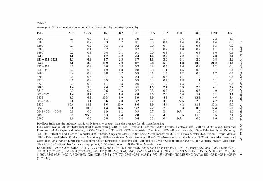
high-technology industries. One approach uses R & D intensity, defined as theratio of R & D to output. We look at two different estimates of this. The first usesan OECD study, ranking industries into high, medium, and low intensity. Thisclassification (based on an OECD average of 11 countries) is available for 1970and 1980 (see Table 2.11, OECD, 1986). In addition, disaggregated country-leveldata for R & D as a percentage of output are available for these countries. Weconstructed an average ranking of R & D as a percentage of output over thesample period for each of these industries by country, as shown in Table 1. Usingthe two measures of R & D intensity, there were three possible ways of definingindustries as high-technology industries. We use the ranking with the highestdomestic relative wage to divide the industries into high- and low-technologyindustries (see Table 2 for details). This follows the approach used by Juhn et al.(1991), who argue that ‘‘skill can be measured in terms of relative productivity, asreflected by an individuals position in the overall distribution of job offers.’’

One limitation is that complete wage and employment data are not available atthe three-digit International Standard Industrial Classification (ISIC) for thesample period, so a two-digit classification was generally used. An exception isfabricated metal products (ISIC 381), for which complete data are available for all

17We could have used many more OECD countries in our sample, but the OECD (1996) database weused in calculating innovation rates only included 15 countries including the United States. Denmark,Belgium and Spain were omitted for data incompleteness.

18For more information on the data and how it was created, see OECD (1992).19For more details on the data, see OECD (1996).20These were converted into ISIC using the concordance study by Jim Kristoff (1992) at the Bureau

of Census.

A.

Butler,

M.

Dueker

/Journal

ofInternational

Econom

ics47

(1999)61

–8971

Table 1Average R & D expenditure as a percent of production by industry by country

ISIC AUS CAN FIN FRA GER ITA JPN NTH NOR SWE UK

3000 0.7 0.9 1.1 1.8 1.9 0.7 1.7 1.6 1.1 2.2 1.73100 0.2 0.2 0.3 0.2 0.1 0.0 0.4 0.4 0.2 0.4 0.33200 0.1 0.2 0.3 0.2 0.2 0.0 0.4 0.2 0.3 0.3 0.23300 0.1 0.1 0.2 0.1 0.2 0.0 0.2 0.0 0.2 0.1 0.13400 0.2 0.3 0.4 0.1 0.1 0.0 0.3 0.1 0.3 0.6 0.13500 1.0 1.0 1.7 2.2 2.4 1.4 2.2 2.2 1.5 2.8 2.13511352–3522 1.1 0.9 1.7 2.5 3.7 1.1 3.0 3.1 2.0 1.8 2.23522 4.0 3.9 10.9 7.0 8.7 5.8 6.6 8.8 10.0 20.2 11.43531354 0.3 0.9 0.6 0.8 0.2 0.3 0.5 0.6 0.2 0.2 0.43551356 0.4 0.3 1.9 1.8 0.8 0.8 1.1 0.5 0.8 1.1 0.43600 0.4 0.2 0.8 0.7 0.5 0.1 1.5 0.2 0.6 0.7 0.53700 0.4 0.6 0.7 0.6 0.4 0.2 0.8 0.7 1.2 1.1 0.43710 0.5 0.3 0.5 0.5 0.5 0.2 0.7 0.8 1.1 1.1 0.43720 0.3 0.9 1.1 0.8 0.5 0.3 1.2 0.3 1.3 1.1 0.43800 1.4 1.8 2.4 3.7 3.1 1.5 2.7 3.3 2.3 4.1 3.43810 0.3 0.2 0.6 0.3 0.7 0.3 0.7 0.3 0.8 1.0 0.3382–3825 1.4 0.7 2.1 1.0 2.0 0.5 2.0 1.0 1.4 3.1 1.13825 1.2 6.8 10.3 6.0 5.9 5.9 4.5 6.3 12.5 4.6 8.4383–3832 0.8 1.1 3.6 2.0 3.2 0.7 3.5 72.5 2.9 4.2 3.13832 52.4 11.5 8.6 10.9 8.6 5.9 4.4 4.2 11.6 12.2 9.23845 0.8 10.5 1.4 14.6 23.2 7.2 7.6 3.3 0.6 12.4 15.038421384413849 0.9 0.8 1.9 1.2 0.9 0.7 2.4 NA 1.5 3.4 1.33850 3.5 NA 8.3 2.4 2.8 0.5 4.0 1.5 11.8 3.5 2.13900 1.0 0.3 0.8 0.4 0.4 0.2 0.4 NA 0.8 0.6 1.0

Boldface indicates the industry has R & D intensity greater than the average for all manufacturing.ISIC Classification: 30005Total Industrial Manufacturing; 31005Food, Drink and Tobacco; 32005Textiles, Footwear and Leather; 33005Wood, Cork andFurniture; 34005Paper and Printing; 35005Chemicals; 3511352–35225Industrial Chemicals; 35225Pharmaceuticals; 35313545Petroleum Refining;35513565Rubber and Plastics Products; 36005Stone, Clay and Glass; 37005Basic Metal Industries; 37105Ferrous Metals; 37205Non-Ferrous Metals;38005Fabricated Metal Products and Machinery; 38105Fabricated Metal Products; 382–38255Non-Electrical Machinery; 38255Office Machinery andComputers; 383–38325Electrical Machinery; 38325Electronic Equipment and Components; 38415Shipbuilding; 38435Motor Vehicles; 38455Aerospace;384213844138495Other Transport Equipment; 38505Instruments; 39005Other Manufacturing.Exceptions: AUS5NO MISSING DATA; CAN5ISIC 385 (1973–92); FIN5ISIC 3845, 38421384413849 (1973–78); FRA5382, 383 (1992); GER5351,352, 383 (1973–76); ITA5330 (1973–79), 351, 352 (1988–92), 3841, 3845, 38421384413849 (1992); JPN5NO MISSING DATA; NTH5371, 372, 382(1992), 38421384413949, 390 (1973–92); NOR53845 (1973–77), 38421384413849 (1973–85); SWE5NO MISSING DATA; UK538421384413849(1973–85).


Table 2Alternative measures of high-technology industries and the relative wages generated

Country Relative Relative RelativeWage 1 Wage 2 Wage 3

Australia 1.15 1.16 1.11Canada 1.14 1.16 1.13Finland 1.03 1.05 1.02France 1.23 1.20 1.07Germany 1.34 1.36 1.23Italy 1.40 1.50 1.38Japan 1.295 1.30 1.23Netherlands 1.17 1.23 1.12Norway 1.15 1.16 1.13Sweden 1.13 1.17 1.12United Kingdom 1.19 1.20 1.13

Where: The high-technology industries in relative wage 1 include ISIC: 35, 38; The high-technologyindustries in relative wage 2 include ISIC: 35, 38–381; The high-technology industries in relative wage3 include ISIC: 38.All other industries are in the low-technology sector.

countries and years. The ranking with the highest average relative wage, given thelevel of aggregation of the data, classified fabricated metal products as a low-technology industry. As a result, the industries are classified as high- and low-techas shown in Table 3.

High-and low-technology workers are measured by a head count of wage andsalary workers and divided into high- and low-tech employment in each countryby the classification discussed above. The data used to calculate the wage gap

Table 3Industry classification

High-technology industries

ISIC 350 Chemical products382 Nonelectric machinery,

office and computing equipment383 Electrical machines384 Transport equipment385 Professional goods

Low-technology industriesISIC 310 Food, beverages and tobacco

320 Textiles, apparel and leather330 Wood products and furniture340 Paper products and printing360 Nonmetallic mineral products370 Basic metal industries381 Fabricated metal products


between high- and low-tech workers are labor costs, which include the costs ofemployer payments for nonwage compensation such as medical coverage andpensions, and represent the total wage bill for that industry for a year. The wagebill per worker is given by summing labor costs over the industries in that sectorand dividing by the total number of workers in that sector for each country. Thedomestic relative wage is thus proxied by the ratio of annual wages per worker inthe high-tech sector relative to the low-tech sector. Fig. 1 plots the relative wagefor all eleven countries. Italy had the largest gap between high-tech and low-techwages throughout the sample period.

Finding an appropriate empirical measure of innovative activity is difficult andhas been discussed at length in the literature. For our purposes we need toconstruct a measure of the productivity of R & D workers. Ideally some standardproductivity measure would be used, such as patents per R & D workers.Complete data on employment of R & D workers are not available for any countryin the sample, however. An alternative, which we use, is the number of patents perdollar of R & D expenditure. This captures some measure of innovative output pereffort (measured in dollars rather than workers). Using patents as a proxy for the‘‘output’’ of R & D workers may be insufficient, because many new goods are notpatented. Nevertheless, patents do provide a means of measuring the degree towhich the production rights of products or processes are exclusive. In general,patents have been found to be a good indicator of unobserved inventive output(see, for example, Griliches, 1990).

A homogeneous unit for measuring the number of patents coming out of thehigh-tech sectors of countries such as Italy and Australia is the number of patents

21their industries filed in the United States.The United States is the largest single market, and most important innovations

are patented in the United States. However, to avoid home country bias, we do not22include the United States in our sample.

The number of U.S. patents taken out by foreign nationals is highly correlatedwith both home-country patenting and R & D intensity, minimizing the costs of

23not using patents filed within the country of origin. Patent data are available bythe date the awarded patent was filed for or the date the patent was received. Wechose to use the date filed, since that is when protection effectively begins.

Therefore, the proxy used for the productivity of R & D workers in each country

21As suggested by Zvi Griliches in conversation. Patents from U.S. companies account for only halfof all patents granted in the United States.

22While we realize this omits an important country, including the United States would overstate itsinnovation rate due to home-country bias. U.S. companies are more likely to file a U.S. patent for aninvention of like quality than a foreign national.

23See Soete and Wyatt (1983). For a discussion on the use of patents as an indicator of innovativeactivity, see Griliches et al. (1987), and Griliches (1990).


Fig. 1. Relative wages: High-tech to low-tech.


24is patents granted per R & D dollar. Foreign innovation is proxied by the totalnumber of patents in the other 10 countries divided by total R & D expenditure inthe other 10 countries. Fig. 2 plots the relative innovation rates for the elevencountries. Italy’s rate of foreign patenting relative to domestic patenting was thehighest throughout the sample. Norway, the smallest country, had the mostvariable relative innovation rate. The variability is not sufficiently great to causesignificant changes in the ranking of Norway’s innovation rate relative to othercountries, however. The small countries generally have more year-to-year variationin their relative innovation rates, due to lumpiness in the number of domesticpatents.

Another parameter from the theoretical model, production worker productivity,presents some challenges for empirical work. The model includes the ratio of laborproductivity in high-tech production to productivity in low-tech production. Theproxy used for the productivity of production workers in each sector is the value ofproduction per worker in that sector. Therefore the ratio of production workerproductivity is given by high-technology output per high-technology workerdivided by output per low-technology worker within the same country. Thismeasure does not perfectly capture differences in labor productivity, because thisratio does not control for capital intensity. No better proxy was available fromavailable international panel data, however, to capture differences in workerproductivity across countries and time.

The parameters characterizing obsolescence, utility and technology transferwere left as constant parameters in our estimated equations and not treated as data.Moreover, as illustrated below, many of these parameters are subsumed in theintercept of the estimated equation, so cross-country differences in the parametersare captured as fixed effects in the panel data.

One feature of innovation and technology transfer not included in this model isthe possibility of spillovers, whereby production of similar goods in one countryleads to spillover effects that make production less costly in other countries.Similar spillovers could take place in R & D, but the sign of the effect is notobvious. If a country undertakes R & D spending on research that is similar innature to spending in another country, the similarity might or might not make iteasier for the second country to generate new designs, patents and unique newgoods from its efforts. Analysis of the effects of possible spillovers within thistype of model is outside the scope of this paper. For this reason, we are able toavoid postulating any measure of ‘‘closeness’’ between goods and countries.

A more serious limitation is that the model does not include capital, so changesin our measure of production worker productivity could be the result of capitaldeepening. However, because the labor productivities only appear as a ratio,

24R & D expenditures were put into dollars using OECD purchasing power parities and thenconverted into 1992 U.S. dollars.


Fig. 2. Relative innovation rates: Domestic to foreign.


capital deepening will not tend to distort the relative productivities to the extentthat capital deepening occurs evenly across these industrialized countries.

4.1. The empirical examination

The section begins by deriving from the product-cycle model the specificationwe estimate. Second, we discuss the econometric methods we use. Third, wepresent and discuss the results in light of the model’s predictions.

5. Specification

The relative wage Eq. (17) is manipulated to have the form of a panel-dataregression equation, which leads to several hypothesis tests related to the model. Amaintained assumption is that the rate of technology transfer is the same acrosscountries in Eq. (17), so that k 5k 5k. We can then write the relative wage as1 2

12uW L1h lu] ]]]]5 f (a /a ) (19)1 lW i1l 2]1L 1 L 2S D1h 2hi1

where12ug(k 1 g 1ur)

]]]]f 5u S D(r 1 k 1 g)k

Rearranging the right hand side of Eq. (18) and taking logs, we obtain

W L i L1h 1h 2 2h] ] ]]ln 5 ln(f) 1u ln(a /a ) 1 (u 2 1)ln 1 (20)S D S D1 lW L i L1l l 1 l

where subscripts h and l denote the high-tech and low-tech industries, respectively.L denotes employment in high-tech industries in the ‘‘rest of the world,’’ i.e., the2h

other countries in the sample, L is worldwide low-tech employment, and il 2

denotes the innovation rate in the rest of the world. Eq. (20) suggests that for eachcountry, the domestic relative high-tech / low-tech wage is a function of theworldwide supply of high-tech workers, measured in innovation-adjusted units ofdomestic high-tech workers, relative to the worldwide endowment of low-techworkers.

Recalling from Eq. (1) that the preference parameter for quantity versus variety,u, is a parameter between zero and one, the model predicts a negative regressioncoefficient on the relative labor supplies equal to (u 21) in Eq. (20). The relativehigh-tech / low-tech labor productivity, proxied by the value of production perworker in the respective sectors, is predicted to have a positive regressioncoefficient equal to u.


We express the last term on the right-hand side of Eq. (20) as components that25separate the foreign and domestic innovation rates:

L i L L1h 2 2h h] ]] ]ln 1 5 ln 1 ln i 2 ln i (21)s d s dS D S D 2 1L i L Ll l l l

with a remainder on the right-hand side, derived from a second order Taylor seriesexpansion, equal to:

2 2L i L i1h 1 1h 1] ] ] ]2 1 2 .5 2 1S DS D S D S DL i L ih 2 h 2

where L is the worldwide supply of high-technology workers.h

This breakdown of the right-hand side variable is necessary to test whetherforeign and domestic innovation rates symmetrically affect the domestic wagedistribution. If the two innovation rates were left as a ratio, the hypothesis of equalinfluence would be maintained without ever being tested.

The specification directly implied by the theoretical model would impose equalcoefficients equal to (u 21) on all of these components, including the remainderterm. The predicted signs for the first three terms are easy to interpret in light ofthe product-cycle model. An increase in the foreign innovation rate diminishes thevalue of domestic R & D workers, whereas an increase in the domestic innovationrate enhances their marginal products. An increase in the worldwide supply ofhigh-tech workers relative to low-tech workers decreases their scarcity and thehigh-tech skills premium in a model in which labor supplies are viewed asexogenous factor endowments. The model-predicted negative sign on the remain-der term is somewhat less intuitive, because the remainder represents a compli-cated nonlinear interaction term between the relative innovation rate and countrysize.

In the regressions, we estimate separate coefficients for each of the fourcomponents from the right-hand side of Eq. (20) and the production workerrelative productivity to test the validity of various model restrictions:

W a L1h 1h 1h] ] ]ln 5 b 1 b ln 1 b ln 1 b ln(i ) 1 b ln(i )S D S DS Do 1 2 3 2 4 1W a L1l l l

2 2L i L i1h 1 1h 1] ] ] ]1 b 2 0.5 (22)FS DS D S D S D G5 L i L ih 2 h 2

Eq. (22) becomes an econometric specification with the addition of a mean zeroerror term. As discussed below, our estimation procedure will make allowances forcorrelation between the explanatory variables and the errors.

Several model-implied restrictions are (from most stringent to least stringent):

25See Appendix A for details.


b 5 b 1 1 and b 5 b 5 2 b 5 b1 2 2 3 4 5

b 5 b 5 2 b 5 b , 0 (23)2 3 4 5

b 5 2 b3 4

The restriction b 52b is a test of the hypothesis that foreign and domestic3 4

innovation rates symmetrically influence the domestic relative wage; that is, thedomestic relative wage would remain unchanged if both innovation rates were todouble or halve. We consider this to be our central hypothesis test and we examineit within the context of a specific model, which is important, because the atheoreticregression we run provides much less significant results than the theoreticspecification.

6. Econometric methods and assumptions

The OECD data set described above provides 20–25 observations per country(22 for the variables and countries in our sample). Because the time span is limitedand the theory is expected to apply to all countries, panel data offer a useful wayto increase the power of statistical tests. Coe and Helpman (1995) and Canzoneriet al. (1996) employ a panel-data approach when working with OECD data sets ofthis size. They also use recently developed results on testing for cointegration inpanel data sets. We follow their use of panel cointegration techniques whenestimating the product-cycle model-based specification. In particular, we usePhillips and Hansen (1990) fully-modified cointegrating least squares estimationand a grouped mean panel estimator, as in Pedroni (1996) and Canzoneri et al.(1996). One highly desirable feature of the Phillips–Hansen procedure is that theerror term can be correlated with the explanatory variables. The Phillips–Hansenprocedure makes several semiparametric adjustments for endogenous regressors,nonstationarity and serially correlated disturbances in cointegrating regressions.Another useful property of Phillips–Hansen fully-modified least squares is that teststatistics have standard t and F distributions. Finally, in panel data, with separatePhillips–Hansen semiparametric adjustments for serial correlation and regressorendogeneity for each country, the dynamics are allowed to be heterogeneousacross countries. Many other treatments of panel data, in contrast, imposehomogeneous dynamics across countries.

To obtain parameter estimates that characterize the panel data set and to utilizethe panel to generate more powerful hypothesis tests, we take the individualcountry parameter estimates and calculate a grouped mean estimate, weighted by


country size (each country’s sample-wide average share of the total number of26workers). The grouped mean estimator is

N]b 5Ov bi k ik

k51

where N is the number of countries in the panel and v is the vector of countryweights that sums to one. Use of the grouped-mean estimator is appropriate whenthe coefficients are assumed to be equal across countries. We test this assumptionin our application. For hypothesis testing, Pedroni (1996) and Im et al. (1995)prove that the grouped mean t-ratio, the properly scaled average of the country-specific t-ratios, is asymptotically standard normal:

20.5] 2t 5 Ov Ov tk k kS Dk k

The scaling factor,

20.52Ov kS Dk

preserves the variance of the t-ratio throughout the averaging process. Some of thehypotheses we wish to test with grouped mean t-ratios embody more than onerestriction. In these cases we take the ‘‘square roots’’ (Cholesky decompositions)of the individual countries’ F-statistics in order to average more than one

27orthogonal t-ratio per country.

7. Empirical results

Fig. 1 shows that for some countries the domestic wage premium has anobvious trend, whereas in others the wage premium simply fails to display signs ofmean reversion. As in Coe and Helpman (1995) and Canzoneri et al. (1996), it isimpossible with data sets of this size to be sure that the data are nonstationary, butwe can at least verify with available tests that the assumption of nonstationarity isnot clearly at odds with the data before applying cointegration methods. We testedthe variables for unit roots using Dickey–Fuller unit root tests for each variable,country by country, with and without time trends. The only instances where theunivariate Dickey–Fuller tests reject a unit root, for Japan only, were its relativeproductivity variable [ln(a /a )] and remainder term. For the other ten countries1h 1l

26One might argue that Norway’s results provide equally important confirmation of the hypotheses asGermany’s. But if the objective is to characterize the competitive situation facing the representativehigh-tech worker, then it seems desirable to weight the observations by country size.

27The t-ratios are asymptotically normal and removing correlation among them via the Choleskydecomposition makes them independent normals.


in all their variables, Dickey–Fuller tests do not find evidence against the nullhypothesis of nonstationarity. Out of nearly 70 univariate unit-root tests in a smallsample, it would not be surprising to have two cases of Type-I error. For thisreason, we pool the data across countries to increase the sample size and decreasethe number of tests performed. The panel unit-root test of Im et al. (1995) followsfrom the argument that the unit-root properties are similar across countries for thesame variable. Table 4 contains the results of this panel unit-root test for the sixvariables used in our study. For all six variables, the null hypothesis of a unit rootis not rejected.

In applying fully-modified least squares, two choices are required. The first isthe lag length to use in estimating the long-run variance–covariance matrix of theregression errors and the disturbances to the explanatory variables. We followed acommon rule of thumb by setting the lag length equal to the integer closest to

1 / 5T , which is two. The second choice is whether to allow for a time trend in thecointegrating relation. Our approach is to estimate with and without the time trendfor each country and include a time trend only for countries where it wassignificantly different from zero.

Table 5 contains the results of applying fully-modified least squares on acountry-by-country basis. The t-statistics for each estimated coefficient are inparentheses. France, Germany, Norway and Japan have significant innovationcoefficients with the expected signs, whereas the Netherlands and the UnitedKingdom have innovation coefficients with the expected signs that are notsignificant. The relative productivity variable is significant for Japan, Canada,Australia, Sweden and Norway, but has the wrong sign for Norway. The relativelabor supply has an equal number (four) of significant negative (expected) andpositive coefficients, making its effect ambiguous across the data set. On acountry-by-country basis, tests of the hypothesis that the foreign innovation ratecarries equal influence with the domestic innovation rate in determining domesticrelative wages [b 52b ] are readily available. Countries where the hypothesis is3 4

rejected are Canada, Finland, Italy, Norway, and Sweden.Before testing specific hypotheses related to the parameter estimates, we verify

Table 4Panel unit root tests from Im et al. (1995)

Critical value to reject is 28.35

Variable Test statistic

Relative wage 21.64Rel. Productivity 23.11Rel. Labor supply 24.98Foreign innov. rate 26.00Domestic innov. rate 22.91Remainder 26.54

82A

.B

utler,M

.D

ueker/

Journalof

InternationalE

conomics

47(1999)

61–89

Table 5Fully modified least squares estimation of product-cycle model t statistics are in parentheses

Country Intercept Rel. prod Lab supply For. innov Dom. innov Remainder Timeb b b b b b trend0 1 2 3 4 5

France 0.452 0.019 0.500 20.534 0.537 24.24(1.74) (0.240) (3.03) (23.01) (2.85) (22.23)

Germany 0.323 0.135 0.354 21.32 1.31 26.03(2.81) (2.04) (7.16) (23.24) (3.20) (23.17)

Italy 0.820 20.001 20.071 0.018 0.035 22.32 0.004(5.53) (20.020) (20.443) (0.230) (0.408) (21.35) (3.24)

Netherlands 0.447 20.022 0.427 21.42 0.144 27.42 20.006(2.28) (20.396) (1.91) (20.532) (0.553) (20.576) (22.76)

UK 20.565 0.148 21.09 20.073 0.038 0.575 0.006(21.77) (1.23) (23.88) (20.737) (0.403) (0.568) (2.43)

Norway 20.130 20.046 20.133 20.114 0.092 218.5(22.30) (24.59) (25.21) (24.59) (3.56) (23.56)

Sweden 20.015 0.385 1.39 0.111 20.195 6.36 20.018(20.043) (3.69) (3.32) (1.50) (22.18) (1.51) (23.63)

Finland 1.14 20.066 1.26 0.357 20.305 43.7 20.013(3.54) (20.774) (4.24) (1.53) (21.24) (1.52) (24.13)

Japan 0.283 0.289 20.569 20.286 0.312 20.791(1.83) (6.65) (26.32) (23.79) (3.76) (24.12)

Canada 0.493 0.178 20.065 0.071 20.033 0.217(2.59) (3.48) (20.653) (0.706) (20.328) (0.118)

Australia 20.425 0.450 20.422 0.322 20.361 13.4(20.856) (4.23) (23.89) (1.90) (22.31) (1.96)


Table 6Country sizes normalized relative to France

Country Relative size

France 1.00Australia 0.239Canada 0.358Finland 0.104Germany 1.76Italy 1.08Japan 2.88Netherlands 0.197Norway 0.066Sweden 0.195United Kingdom 1.25

that the null of no cointegration is rejected for the panel. Pedroni (1995) presents apanel-data cointegration test based on a panel analogue of the Phillips and Perron(1988) test. Canzoneri et al. (1996) also apply this cointegration test in their workand generalize the test for the case where not all cross-sectional units have thesame number of observations. Pedroni (1995) tabulates critical values for the test,based on the number of observations and the cross-sectional dimension. Pedroni’sTable B.3 suggests a critical value at the one percent probability level of 28.43.Our cointegrating residuals give a test statistic of 213.7, so we can easily rejectthe null of no cointegration in our panel.

Table 6 contains the vector of relative country sizes, as measured by acountry’s average share of the total number of workers throughout the sampleperiod. The relative country sizes are used to weight the estimates in forming thegrouped mean coefficient estimates. Table 7 presents the grouped mean coefficientestimates and their corresponding grouped mean t-ratios. We examine results forthree country groupings. The first is the sample of all eleven countries. The second

Table 7Grouped mean coefficient estimates with t-ratios in parentheses

Coefficient Full sample Euro1Japan Euro only

rel prod 0.165 0.157 0.089b (6.00) (5.36) (2.33)1

lab sup 20.175 20.173 0.029b (23.10) (22.87) (0.374)2

for innov 20.397 20.437 20.515b (24.60) (24.74) (23.84)3

dom innov 0.405 0.445 0.513b (4.61) (4.75) (3.80)4

remain 21.37 21.85 22.39b (21.99) (22.62) (22.25)5


Table 8Grouped mean t-ratios for equal coefficients across countries

Coefficient Full sample Euro1Japan Euro only

rel prod 0.141 0.079 20.501lab sup 3.21 3.05 3.95for innov 21.26 21.38 21.26dom innov 1.55 1.67 1.46remain 21.51 22.04 21.82

is for Europe plus Japan and the third is for European countries only. For the fullsample, all five coefficients have the expected signs and are significant. Thegrouped mean coefficient estimates are estimated with considerably greaterprecision than coefficients for individual countries.

The validity of the grouped mean coefficient estimates rests, however, on thehypothesis that each coefficient has the same value for all countries, so that for b ,1

28for example, b 5b ; j, k. Table 8 contains grouped mean t-ratios testing this1j 1k

hypothesis for each coefficient and suggests that, with the exception of the laborsupply coefficient, it is plausible to treat the grouped mean coefficient estimates asrepresentative of the data set as a whole. We might have expected to find evidenceof heterogeneous coefficients on the relative labor supply, because we have bothhighly significant positive and negative coefficients in the country-by-countryestimates.

We therefore discuss the grouped mean parameter estimates from Table 7 withsome confidence that they characterize the panel as a whole. For the full sampleand the sample of Europe1Japan, all coefficients have the model-implied signsand are significant. Using only the eight European countries, the innovationcoefficients remain highly significant with the right signs. The labor supplycoefficient, on the other hand, changes sign and is very close to zero. The relativeproductivity coefficient remains significant, although its t-statistic falls by half.Thus, the inclusion of Japan appears to influence some of the grouped meanparameter estimates significantly, but less so in the innovation coefficients. Table 9

Table 9Grouped mean t-ratios for coefficient restrictions across all countries

Hypothesis Full sample Euro1Japan Euro only

b 52b 1.88 1.75 0.5023 4

b 5b 52b 5b 25.75 25.92 22.342 3 4 5

b 5b 11 and1 2

b 5b 52b 5b 214.4 214.8 217.52 3 4 5

28Note that many applications of grouped mean estimators do not include this diagnostic test.


presents grouped mean t-statistics for three model-implied coefficient restrictionsfrom Eq. (23). Equal absolute innovation coefficients are not rejected for any ofthe three country groupings, but the broader model-implied restrictions are allrejected. The coefficients on relative productivity are all too low to have a unitdifference from the others. Similarly the coefficient on the remainder is generallytoo large to be equal to the innovation coefficients. For this reason, we checkwhether the coefficient on the remainder term is so large as to cause implausibleestimates of the average innovation elasticities.

The elasticity of the domestic relative wage with respect to the innovation ratesis

≠ln(w /W )h l]]]] (24)

≠ln(i )1

which depends on the derivative of the remainder with respect to i and, therefore,1

varies with country size and the relative innovation rate. We report an elasticity forthe ‘‘average’’ country for which i /i 51 and L /L 51/N, where N is the1 2 1h h

number of countries in the sample. In this case, the elasticities are

≠ln(w /w )h l]]]5 b 1 b /N (25)4 5≠ln(i )1

≠ln(w /w )h l]]]5 b 2 b /N (26)3 5≠ln(i )2

The sum of the average elasticities is zero under the hypothesis that b 52b .3 4

Panel-wide estimates of the ‘‘average’’ innovation elasticities are in Table 10. Incontrast to the instability in the coefficients on relative productivity and relativelabor supply depending on whether or not Japan is in the sample, the averageinnovation elasticities are quite stable across country groupings, with and withoutJapan. A robust finding is that an increase in the domestic innovation rate by tenpercent would lead to an increase in the domestic relative wage by more than twopercent in a country with an average number of workers and the average

Table 10Innovation elasticities for the effect of foreign and domestic innovation rates on the domestic relativewage

Elasticity Full sample Euro1Japan Euro only

domesticb 1b /N 0.280 0.239 0.2144 5

foreignb 2b /N 20.272 20.232 20.2153 5

sumb 1b 0.008 0.007 20.0013 4


Table 11Product-cycle model versus atheoretical regression with t-ratios in parentheses

Coefficient Full sample Euro only

model atheor model atheor

rel prod 0.165 0.153 0.089 0.065b (6.00) (4.64) (2.33) (1.49)1

lab sup 20.175 20.318 10.029 20.036b (23.10) (26.11) (0.374) (20.522)2

for innov 20.397 20.029 20.515 20.038b (24.60) (21.47) (23.84) (21.58)3

dom innov 0.405 0.023 0.513 0.029b (4.61) (1.24) (3.80) (1.45)4

remain 21.37 22.39b (21.99) (22.25)5

innovation rate. A corresponding increase in the foreign innovation rate would alsolower the domestic relative wage by essentially the same amount.

Having rejected several of the model-implied coefficient restrictions, but not thebasic proposition of cointegration and the importance of and symmetry betweenforeign and domestic innovation, a question remains: Does the product-cyclemodel simply help us identify variables that enter a cointegrating relationship? Inother words, would an atheoretical regression provide equally significant results?Using the product-cycle model simply to identify relevant variables for anatheoretical regression specification would lead one to include relative productivi-ty, the relative labor supply and the innovation rates. Thus, an atheoreticalspecification would include everything except the remainder term. For this reason,we examine results for a specification that omits the remainder term. Table 11provides the comparison and shows that the innovation rates lose their significanceif they do not interact with the remainder term. In particular, one would concludethat the elasticity of the domestic relative wage with respect to either innovationrate is essentially zero. The product-cycle model, on the other hand, implies aspecification in which the importance of the innovation rates becomes apparent.

8. Conclusions

This paper uses industry-level data from 11 advanced countries to carry outempirical tests of several propositions regarding domestic high-tech / low-techwages stemming from a product-cycle model. The most novel empirical finding isthe importance of foreign innovation in the high-tech sector in determining thedomestic relative wage. While there has been much rhetoric surrounding the effectsof increased competition in high-technology industries, these results demonstrateempirically how domestic and foreign innovation affect domestic wages in


high-technology industries. We find that foreign innovation has a significantnegative effect on the relative wage between domestic high- and low-tech workers.Similarly, an increase in domestic innovation has a significant positive effect onthe domestic wage differential. The latter result is consistent with the results ofMincer (1991) for the United States and provides more rigorous evidence for theargument discussed by Davis (1992) and elsewhere that domestic proficiency intechnological innovation, relative to foreign competitors, plays a significant role indetermining domestic relative wages. We find that increases in the foreigninnovation rate and in the domestic innovation rate impact domestic relative wagesby roughly equal and opposite magnitudes, as predicted by the product-cyclemodel.

Acknowledgements

We would like to thank Hassan Arvin-Rad, Peter Pedroni, Patricia Pollard,Robert Witt, Participants in the Macroeconomic Workshop at George WashingtonUniversity, the coeditor Jim Levinsohn and an anonymous referee for usefulcomments. The views expressed are those of the authors and do not necessarilyreflect official positions of the Federal Reserve Bank of St. Louis or the FederalReserve System.

Appendix A

To derive the breakdown of the variable in Eq. (21), we start with the followingidentity:

L i L i L i L1h 2 2h 2 1h 1 2h] ]] ] ] ] ]ln 1 5 ln 1 ln 1 ln 1S D S D S D S DL i L i L i Ll 1 l 1 l 2 1h

and take a second-order Taylor series approximation to

i L L L1 2h 2h h] ] ] ]ln 1 around the point ln 1 1 5 lnS D S D S Di L L L2 1h 1h 1h

Under the approximation,

2 2i L L L i L i1 2h h 1h 1 1h 1] ] ] ] ] ] ]ln 1 ¯ ln 1 2 1 2 0.5 2 1S D S D S D S D S Di L L L i L i2 1h 1h h 2 h 2

The term

2 2L i L i1h 1 1h 1] ] ] ]2 1 2 0.5 2 1S D S D S DL i L ih 2 h 2


is what we have called the remainder term, so we end up with the breakdown inEq. (21):

L i L L1h 2 2h h] ]] ]ln 1 ¯ ln (i ) 2 ln (i ) 1 ln 1 remainder.S D S D2 1L i L Ll 1 l l

References

Berman, E., Bound, J., Griliches, Z., 1994. Changes in the demand for skilled labor within U.S.manufacturing industries: Evidence from the annual survey of manufacturing. Quarterly Journal ofEconomics 109, 367–397.

Burtless, G., 1995. International trade and the rise of earnings inequality. Journal of EconomicLiterature 33, 800–816.

Butler, A., 1997. Product cycles and domestic wage inequality in innovating countries. CanadianJournal of Economics 30, 1007–1026.

Canzoneri, M., Cumby, R., Diba, B., 1996. Relative labor productivity and the real exchange rate in thelong run: evidence for a panel of OECD countries. NBER Working Paper No. 5676.

Coe, D.T., Helpman, E., 1995. International R & D spillovers. European Economic Review 39,859–887.

Davis, S.J., 1992. Cross-country patterns of change in relative wages. In: Blanchard, O., Fischer, S.(Eds.), NBER Macroeconomics Annual 1992. MIT Press, Cambridge, pp. 239–291.

Griliches, Z., 1990. Patent statistics as economic indicators: A survey. Journal of Economic Literature28, 1661–1707.

Griliches, Z., Pakes, A., Hall, B.H., 1987. The value of patents as indicators of inventive activity. In:Dasgupta, P., Stoneman, P. (Eds.), Economic Policy and Technological Performance. CambridgeUniversity Press, pp. 97–124.

Grossman, G.M., Helpman, E., 1991. Quality ladders in the theory of growth. Review of EconomicStudies 58, 43–61.

Grossman, G.M., Helpman, E., 1991. Quality ladders and product cycles. Quarterly Journal ofEconomics 106, 557–586.

Im, K., Pesaran, M.H., Shin, Y., 1995. Testing for unit roots in heterogeneous panels. Working paper,Department of Applied Economics, Cambridge University.

Juhn, C., Murphy, K.M., Topel, R.H., 1991. Why has the natural rate of unemployment increased overtime? Brookings Papers on Economic Activity, 75–126.

Katz, L.F., Murphy, K.M., 1992. Changes in relative wages, 1963–1987: Supply and demand factors.Quarterly Journal of Economics 107, 35–78.

Kosters, M.H., 1994. An overview of changing wage patterns in the labor market. In: Bhagwati, J.,Kosters, M.H. (Eds.), Trade and Wages: Leveling Wages Down? American Enterprise Institute,Washington, DC.

Kristoff, J., 1992. United States industries standard industrial classification regrouped to internationalstandard classification. Mimeo.

Mincer, J., 1991. Human capital, technology, and the wage structure: What do time series show? NBERWorking Paper No. 3581.

OECD, DSTI (ANBERD database), 1996.OECD, Employment Outlook, (July 1993).OECD, DSTI (STAN/Industrial Database), 1992.OECD, 1986. OECD Science and Technology Indicators, No 2: R & D, Invention and Competitiveness,

1986.


Pedroni, P., 1995. Panel cointegration: Asymptotic and finite sample properties of pooled time seriestests and application to the PPP hypothesis. Indiana University working paper.

Pedroni, P., 1996. Fully modified OLS for heterogeneous panels. Indiana University working paper.Phillips, P.C.B., Hansen, B.E., 1990. Statistical inference in instrumental variables regression with I(1)

processes. Review of Economic Studies 57, 99–126.Phillips, P.C.B., Perron, P., 1988. Testing for a unit root in the time series regression. Biometrika 75,

335–346.Soete, L.G., Wyatt, S.M.E., 1983. The use of foreign patenting as an internationally comparable science

and technology output indicator. Scientometrics 5, 31–54.Stafford, F.P., Johnson, G.E., 1993. International competition and real wages. American Economic

Review 83, 127–130.Young, A., 1993. Substitutability and complementarity in endogenous innovation. Quarterly Journal of

Economics 108, 775–807.

does foreign innovation affect domestic wage inequality?

Documents