does composition of public expenditure matter

Does Composition of Public Expenditure Matter for Economic Growth? Lessons from Sri Lanka

Real Wages, In�ation and Labour Productivity: Evidence from the Public and Private Sectors in Sri Lanka

Determinants of Micro�nance Interest Rates: Case of Sri Lanka

- Mayandy Kesavarajah

- Rohini D. Liyanage

- Indeewari U. Colombage and Tharanga A.D. Wijayakoon

27

59

Volume 49

No. 02 - 2019

Volume 49 No. 2 – 2019

CENTRAL BANK OF SRI LANKA

STAFF STUDIES

ii

ISSN 1391 – 3743

The views presented in the papers are those of the authors and do not necessarily indicate the views of the Central Bank of Sri Lanka.

iii

Research Advisory Panel of the Economic Research Department

Dr. C Amarasekara (Director of Economic Research, Chair)Dr. P K G HarischandraDr. D S T WanaguruDr. E W K J B EhelepolaDr. S JegajeevanDr. L R C PathberiyaDr. M M J D MaheepalaDr. S P Y W Senadheera

List of External Reviewers

Mr. Adam Remo (International Monetary Fund)Dr. Ananda Jayawickrama (University of Peradeniya) Mr. Ananda Silva (Central Bank of Sri Lanka, retired)Mr. K D Ranasinghe (Central Bank of Sri Lanka, retired)Dr. Koshy Mathai (International Monetary Fund)Dr. Manuk Ghazanchyan (International Monetary Fund) Dr. Missaka Warusawitharana (Federal Reserve System –USA)Prof. Nelson Perera (University of Wollongong)Prof. Prema-chandra Athukorale (Australian National University)Dr. Rahul Anand (International Monetary Fund) Dr. Shirantha Heenkenda (University of Sri Jayewardenepura)Prof. Sirimewan Colombage (Open University of Sri Lanka)Dr. T Vinayagathasan (University of Peradeniya)Prof. Sunil Chandrasiri (University of Colombo)

Editorial Committee

Dr. C Amarasekara (Editor)Mr. K R D Koswatte (Assistant Editor)Mr. S M Rajakaruna (Assistant Editor)

For all correspondence about the Staff Studies Journal, please contact:

Director of Economic ResearchCentral Bank of Sri Lanka30, Janadhipathi MawathaColombo 01Sri LankaEmail: [email protected]

11


Mayandy Kesavarajah 1

Abstrac t

In the context of surging public expenditure and crumbling output growth, the growth effects of public expenditure have provoked an extensive discussion in the economic and political arenas in Sri Lanka. Since 1977, both public expenditure and its composition have changed intensely and largely been accompanied by expansion in size of successive governments. Although it is difficult to determine whether Sri Lanka has reached its optimal size of public expenditure, understanding the growth effects of public expenditure would clearly link policy contributions made by public expenditure in spurring growth in Sri Lanka. The purpose of this study is to examine the growth effects of composition of public expenditure considering full implications of government budget constraints. This study considers public expenditure at a disaggregated level to isolate productive elements of public expenditure from the total. Accordingly, public expenditure on education, health, defence, agriculture and transport and communication are considered. These expenditure items are selected based on their share in total expenditure. This study found that the growth effects of public expenditure vary at disaggregated levels. A major finding showed that public expenditure in education, agriculture, transport and communication sectors is positively and significantly associated with economic growth while defence and health expenditure do not have any significant impact on growth. Given the high magnitude of positive and significant growth effects of public expenditure in the education sector, this study suggests reforming public expenditure in favour of human capital development is paramount to stimulate long-term growth in Sri Lanka.

Key Words : Public Expenditure, Economic Growth, Government Budget

JEL Class i f i ca t ion : H50, O40, H60

1 The author is currently serving as a Senior Economist at the Economic Research Department of the Central Bank of Sri Lanka. The author is grateful to Dr Katsushi Imai and Dr Yin-Fang Zhang of the University of Manchester, United Kingdom and anonymous reviewers for their valuable comments and suggestions in developing this research paper. The author also would like to thank Dr Chandranath Amarasekara, Director of Economic Research and the Chairman of the Research Advisory Panel, Mr K R D Koswatte, Mrs N S Hemachandra and Mr S M Rajakaruna of the Central Bank of Sri Lanka for their support and encouragement. The views expressed in this paper are those of the author and do not necessarily reflect those of the Central Bank of Sri Lanka. Corresponding email: [email protected]


Mayandy Kesavarajah1

Abstract

Key Words: Public Expenditure, Economic Growth, Government Budget

JEL Classification: H50, O40, H6

Central Bank of Sri Lanka – Staff Studies – Volume 49 Number II - 2019

2

2

1. Introduction

In the recent years, the growth effects of size and the nature of public expenditure have emerged as a major issue in economies that are in transition. Public expenditures are less flexible than fiscal revenues, but much more sensitive with regard to business cycles and policy decisions of the government. Government collects revenue through various taxes and allocates to several sectors of the economy to pursue number of objectives. However, allocation of such expenditures is directly and indirectly associated with growth in the respective economies (Barro, 1990; Tanzi and Zee, 1997; Bayraktar, et al. 2015). For instance, the supply of social and physical infrastructure, rule of law, and protection of property rights are assumed to be conducive for growth (Ram, 1986). Over the period, public expenditure policies in both advanced and emerging economies mainly aimed at promoting sustained and equitable economic growth. However, literature highlights growth effects of public expenditure are positive when the size of government is small, but it may become negative as the size gets larger (Grossman and Helpman, 1991).

In the context of surging public expenditure and crumbling output growth, the growth effects of public expenditure have provoked an extensive discussion in the economic and political arenas of Sri Lanka. Since 1977, both public expenditure and its composition have changed intensely and largely been accompanied by expansion in size of successive governments (Figure A2 in Appendix). However, on the empirical front, the existing studies for Sri Lanka (Herath, 2010; Lahirushan, and Gunasekara, 2015; Dilrukshini, 2004) have focused on either the growth effects of total public expenditure or the specific individual expenditure. To the best of our knowledge, a few studies have examined the growth effects of public expenditure at disaggregated levels (Kesavarajah, M and Ravinthirakumaran, N, 2011). This study, therefore, attempts to fill an existing gap in the literature in light of more recent evidence.

The present study departs from existing literature in four key aspects. First, this study uses a time series dataset covering the entire post-liberalization period from 1977 to 2016 and places special focus on the presence of structural breaks in both public expenditure and economic growth series1. Secondly, public expenditure will be used as opposed to government consumption expenditure. Thirdly, this study will consider public expenditure at a disaggregated level to isolate productive elements of public expenditure from total. Finally, the analytical approach adopted in this study will be different from previous studies.

Although it is difficult to determine whether Sri Lanka has reached its optimal size of public expenditure, understanding the growth effects of public expenditure would clearly link policy contribution made by public expenditure in spurring growth. Therefore, the main research

1 Sri Lankan economy was liberalised in 1977. The study period covered in this study contains two important break periods. First, the civil war started in 1983 ended in 2009. And second, the global financial crisis which emerged in 2008.

2nd Proof17/07/2020

3


3

question this study attempts to address is: have growing public expenditure really helped in stimulating economic growth in Sri Lanka. In addressing this question, a fundamental issue then is what components of public expenditure might be conducive or detrimental to economic growth in Sri Lanka? This study aims to provide fresh empirical insights for these research questions. Given the research questions, the primary objective of this study is to examine the growth effects of components of public expenditure in Sri Lanka. In this study, public expenditure on education, health, defense, agriculture and transport and communication are considered. These expenditure items are selected based on their share in total expenditure.

The rest of this paper is structured as follows. Section two briefly reviews theoretical and empirical literature relating to the relationship between public expenditure and economic growth. Section three highlights the data, econometric models and analytical framework adopted in this study. Section four offers quantitative insights on growth effects of both total and components of public expenditure. Final section summarizes major findings of the study, recommends appropriate policy responses, and suggests avenues for further research.

2. Literature review

2.1 Theoretical review

There are three main theories, namely Wagner’s law, Keynesian growth theory and endogenous growth theory, which discuss theoretical relationships between public expenditure and economic growth. According to Wagner’s law, public expenditure is an endogenous factor driven by growth of national income. It further states that economic activities undertaken by the government upsurges compared to the private sector during economic development (Wagner, 1883). In contrast, Keynesian growth theory (1936) considers public expenditure as an important exogenous variable in determining growth. It argues, given the assumption of price rigidity and possibility of excess capacity, expansion in fiscal policy stimulates growth through growing aggregate demand, which affects technical progress. Although both theories focus on short-run phenomenon of public expenditure, the causality between public expenditure and growth highlighted by these theories is different. According to Keynesian growth theory, causality runs from public expenditure to growth. Wagner’s law presents the opposite conclusion. However, several studies including Devarajan, et al. (1996), Afonso and Furceri (2008) and Bose et al. (2007) highlight that the nexus between public expenditure and growth depends on the nature of the expenditure. The endogenous growth theory highlights important factors that contribute to cross-country differences in both per capita income and growth rates. These factors comprise, investment in human capital (Lucas, 1988), knowledge spillovers, and investment in physical infrastructure. This theory argues that government’s policies, including fiscal policy, can

3

question this study attempts to address is: have growing public expenditure really helped in stimulating economic growth in Sri Lanka. In addressing this question, a fundamental issue then is what components of public expenditure might be conducive or detrimental to economic growth in Sri Lanka? This study aims to provide fresh empirical insights for these research questions. Given the research questions, the primary objective of this study is to examine the growth effects of components of public expenditure in Sri Lanka. In this study, public expenditure on education, health, defense, agriculture and transport and communication are considered. These expenditure items are selected based on their share in total expenditure.

The rest of this paper is structured as follows. Section two briefly reviews theoretical and empirical literature relating to the relationship between public expenditure and economic growth. Section three highlights the data, econometric models and analytical framework adopted in this study. Section four offers quantitative insights on growth effects of both total and components of public expenditure. Final section summarizes major findings of the study, recommends appropriate policy responses, and suggests avenues for further research.


2.1 Theoretical review

There are three main theories, namely Wagner’s law, Keynesian growth theory and endogenous growth theory, which discuss theoretical relationships between public expenditure and economic growth. According to Wagner’s law, public expenditure is an endogenous factor driven by growth of national income. It further states that economic activities undertaken by the government upsurges compared to the private sector during economic development (Wagner, 1883). In contrast, Keynesian growth theory (1936) considers public expenditure as an important exogenous variable in determining growth. It argues, given the assumption of price rigidity and possibility of excess capacity, expansion in fiscal policy stimulates growth through growing aggregate demand, which affects technical progress. Although both theories focus on short-run phenomenon of public expenditure, the causality between public expenditure and growth highlighted by these theories is different. According to Keynesian growth theory, causality runs from public expenditure to growth. Wagner’s law presents the opposite conclusion. However, several studies including Devarajan, et al. (1996), Afonso and Furceri (2008) and Bose et al. (2007) highlight that the nexus between public expenditure and growth depends on the nature of the expenditure. The endogenous growth theory highlights important factors that contribute to cross-country differences in both per capita income and growth rates. These factors comprise, investment in human capital (Lucas, 1988), knowledge spillovers, and investment in physical infrastructure. This theory argues that government’s policies, including fiscal policy, can


4

4

affects long-run growth. Although these theories highlight that public expenditure affects growth in several channels, empirically, however, each channel leads to varied conclusions.

2.2 Empirical evidence

Beyond theoretical outpourings, several empirical studies have investigated growth effects of public expenditure in both developed and developing economies. However, findings of these studies have brought inconclusive results. Some studies show that public expenditure has positive impacts on growth while others show detrimental impacts. Studies have also found neutral growth effects of public expenditure. Differences in outcome could be largely due to the nature of data and differences in econometric techniques. A study conducted by Barro (1990) integrating both developed and developing economies for the period 1960 to 1985 shows that the nexus between public expenditure and growth is weak. Komain and Brahmasrene (2007) focusing on Thailand find a significant positive impact of public expenditure on growth. They also highlight that a unidirectional causality goes from public expenditure to growth. Using cross section data for 71 countries, Cooray (2009) shows that the growth effects of both government size and quality of governance are positive. Castles and Dowrick (1990) use composition of public expenditure and find that social transfers and education expenditure have a positive impact on economic growth. A similar study was conducted by Ranjan and Sharma (2008) for the case of Indian economy and found growth effects of public expenditure to be positive and significant during the period 1950 to 2007.

Tanzi and Zee, (1997) find that public expenditure on infrastructure, human capital, science and technology influences positively on economic growth. Avila and Strauch (2003) show that the expenditure side of budget consistently affected growth in 15 member countries in European Union for the period 1960 to 2001. The study argues that investment expenditure had positive impacts on growth but expenditure on consumption and transfer payments had significant negative impacts on growth. However, Levine and Renelt (1992) show that growth effects of public expenditure are insignificant. Similarly, Devarajan, et al. (1996) investigate growth effects of various types of public expenditure and highlighted components of public expenditure matters for growth.

Although many studies establish positive growth effects of public expenditure, studies also showed opposite results. A study conducted by Folster and Henrekson (2001) for Organization for Economic Cooperation and Development (OECD) countries highlight negative growth effects of public expenditure. They show countries experienced with higher public expenditure registered lower output growth compared with countries registered low public expenditure. Ramayandi (2003) found adverse impacts of increased public expenditure on growth in Indonesia. Conducting a research for a sample of 96 countries,

4

affects long-run growth. Although these theories highlight that public expenditure affects growth in several channels, empirically, however, each channel leads to varied conclusions.

2.2 Empirical evidence

Beyond theoretical outpourings, several empirical studies have investigated growth effects of public expenditure in both developed and developing economies. However, findings of these studies have brought inconclusive results. Some studies show that public expenditure has positive impacts on growth while others show detrimental impacts. Studies have also found neutral growth effects of public expenditure. Differences in outcome could be largely due to the nature of data and differences in econometric techniques. A study conducted by Barro (1990) integrating both developed and developing economies for the period 1960 to 1985 shows that the nexus between public expenditure and growth is weak. Komain and Brahmasrene (2007) focusing on Thailand find a significant positive impact of public expenditure on growth. They also highlight that a unidirectional causality goes from public expenditure to growth. Using cross section data for 71 countries, Cooray (2009) shows that the growth effects of both government size and quality of governance are positive. Castles and Dowrick (1990) use composition of public expenditure and find that social transfers and education expenditure have a positive impact on economic growth. A similar study was conducted by Ranjan and Sharma (2008) for the case of Indian economy and found growth effects of public expenditure to be positive and significant during the period 1950 to 2007.

Tanzi and Zee, (1997) find that public expenditure on infrastructure, human capital, science and technology influences positively on economic growth. Avila and Strauch (2003) show that the expenditure side of budget consistently affected growth in 15 member countries in European Union for the period 1960 to 2001. The study argues that investment expenditure had positive impacts on growth but expenditure on consumption and transfer payments had significant negative impacts on growth. However, Levine and Renelt (1992) show that growth effects of public expenditure are insignificant. Similarly, Devarajan, et al. (1996) investigate growth effects of various types of public expenditure and highlighted components of public expenditure matters for growth.

Although many studies establish positive growth effects of public expenditure, studies also showed opposite results. A study conducted by Folster and Henrekson (2001) for Organization for Economic Cooperation and Development (OECD) countries highlight negative growth effects of public expenditure. They show countries experienced with higher public expenditure registered lower output growth compared with countries registered low public expenditure. Ramayandi (2003) found adverse impacts of increased public expenditure on growth in Indonesia. Conducting a research for a sample of 96 countries,

2nd Proof17/07/2020

5


5

Landau (1983) concluded expenditure on education and defense sectors has a weak impact on growth. He also confirmed that growth effects of total expenditure are negative.

Few studies have examined growth effects of public expenditure in Sri Lanka and results are inconclusive. Herath (2010) covering the period 1959 to 2003 found positive and significant impacts of public expenditure on economic growth. He also confirms positive growth effects of openness. Similar results have been established by Lahirushan and Gunasekara (2015) while confirming bidirectional causality between public expenditure and growth. Meanwhile, Jayawickrame (2004) stresses reduction in government consumption expenditure, transfer payments and investment expenditure, which have adverse impacts on growth. However, Dilrukshini (2004) shows that there is no empirical evidence in support of either Wagner’s Law or the Keynesian hypothesis in Sri Lanka.

3. Data, econometric models and analytical framework

3.1 Data This study uses time series annual data for the period 1977 to 2016. The data on fiscal variables are mainly based on annual reports of the Central Bank of Sri Lanka (CBSL). Data for other variables have been extracted from three different sources. Growth rates of GDP and gross fixed capital formation are mainly drawn from World Development Indicators. Further, growth rates of population and inflation are drawn from various publications of the Department of Census and Statistics (DCS) of Sri Lanka. The data on human capital variables are drawn from Barro and Lee (2000) data set. Detailed explanation on variables and their sources are given in Table A1 in Appendix.

3.2 Econometric models The analysis of this study will be based on the standard growth regression model. The standard growth regression model, which follows seminal contribution of Barro (1990), has been widely used in empirical research on economic growth. This model is based on a conditional convergence equation that relates output growth to initial levels of income, investment, human capital and population growth. However, to achieve the main objective of the present study, we augment standard growth regression model with both fiscal and non-fiscal variables. Accordingly, the basic empirical model is specified as follows.

!"! = !! + !!!!

!

!!!

+ !!!!

!

!!!

+ !!!!

!

!!!

+ Ԑ! (1)

5






!"! = !! + !!!!

!

!!!

+ !!!!

!

!!!

+ !!!!

!

!!!

+ Ԑ! (1)

5






!"! = !! + !!!!

!

!!!

+ !!!!

!

!!!

+ !!!!

!

!!!

+ Ԑ! (1)


6

6

Where, t is the year index, GR is the growth rate of real GDP, !! and !! are coefficients in regression model. Ԑ! is the error term assumed to be white noise process. Growth rate of real GDP is dependent variable and explanatory variables are classified into three groups: X, Y and Z. Group X consists of conditioning variables that are commonly appears in growth regression model, while group Y includes non-fiscal control variables that are generally included in empirical literature on economic growth. Fiscal variables that we are interested in this study are included in group Z.

Consistent with advocates of growth theory, we include gross investment, growth rate of population and human capital as conditioning variables. Although inclusion of different control variables results to different outcomes, the selections of control variables in this study are based on growth literature. As many countries registered higher growth consistent with export-led strategies, we include trade openness as the control variable. Following Easterly and Rebelo (1993), we include broad money and inflation to capture growth effects of monetary policy and macroeconomic instability. Further, lagged value of economic growth is included to capture growth inertia factors. We also introduce a dummy variable to examine the impacts of civil war on growth.

As Sri Lanka is confronted with fiscal constraints over the periods, we considered government budget constraints to eliminate coefficient bias resulting from their omission (Bose et al. 2007). Accordingly, we include public expenditures, tax revenues and fiscal balance to growth regression model. We also exclude some expenditure items to avoid any multicollinearity problem. As there is a time lag between the execution of public expenditure and its propagation on economy, we consider lagged value of public expenditure in the model.

Since we aim to examine growth effects of both total and components of public expenditure, we first estimate growth effects of total public expenditure as specified in equation 2 and then we jointly include five components of public expenditure as given in equation 3 to isolate productive elements of public expenditure from total.

!"! = !! + !!!!!!!! + !!!!

!!!! + !!!"#! + !!!!! + !!!"!+!!!"!!! +

!!!"#$! + !!

(2)

!"! = !! + !!!!!!!! + !!!!

!!!! + !!!"#! + !!!"#! + !!!"#! + !!!"! +

!!!"#! + !!!"! + !!!"!+!!!"!!! + !!!"#$! + !! (3)

(2)

2nd Proof17/07/2020

7


7

3.3 Analytical framework The analysis of this study will be conducted in five stages. Given that our sample involves the period around the end of the civil war in 2009 and the emergence of global financial crisis in 2008, we will first investigate structural changes in both economic growth and public expenditure series. The global maximiser test introduced by Bai and Perron (2003) will be used to determine any structural breaks.

As many time series variables contain unit root, in the second stage, we will examine stationary properties of all the variables using Augmented Dickey Fuller (ADF), Phillips Perron (PP) and Kwiatkowski-Phillips-Schmidt-Shin (KPSS) tests. We will use Akaike Information Criteria (AIC) with default lag order for selecting order of augmentation in ADF regression. Further, default settings of Bartlett Kernel and Newey-West Bandwidth will be used for KPSS tests.

Although Engel-Granger (1987) and Johenson and Juselious (1990) methods are widely used to examine co-integration among variables, these techniques are not reliable for small sample size and may not provide co-integration even when all variables are integrated with order I(1) (Kremers at el, 1992). Therefore, in the third stage, we will use the Autoregressive Distributed Lag (ARDL) approach introduced by Pesaran and Pesaran (1997) to examine long-run dynamics among variables. This approach can be applied even when variables are I(0) or I(1) or mixture of both. It also considers adequate number of lags to capture data generating process. Given the scope of this study, the ARDL model is specified as follows.

∆!"! = !! + !!!"!!! + !!!!!! + !!!!!! + !!!!!! + !!∆!"!!!!!!! +

!!∆!!!!!!!! + !!∆!!!!

!!!! + !!∆!!!!

!!!! + !!!"#$! + Ԑ! (4)

Equation 4 estimates (p+1)k number of regressions to obtain optimal lag length for each variable in the model. Where, p is the optimal lag to be used and k is the number of variables. ∆ is the first difference operator. As Schwarz Information Criteria (SIC) is widely known as parsimonious model and selects smallest possible lag length, we will use SIC to select optimal lag length in this study. If variables are found to be co-integrated, we will estimate ARDL Error Correction Model (ECM) to investigate short-run dynamics among variables. The error correction version of modified ARDL model is specified as follows.

7

3.3 Analytical framework The analysis of this study will be conducted in five stages. Given that our sample involves the period around the end of the civil war in 2009 and the emergence of global financial crisis in 2008, we will first investigate structural changes in both economic growth and public expenditure series. The global maximiser test introduced by Bai and Perron (2003) will be used to determine any structural breaks.

As many time series variables contain unit root, in the second stage, we will examine stationary properties of all the variables using Augmented Dickey Fuller (ADF), Phillips Perron (PP) and Kwiatkowski-Phillips-Schmidt-Shin (KPSS) tests. We will use Akaike Information Criteria (AIC) with default lag order for selecting order of augmentation in ADF regression. Further, default settings of Bartlett Kernel and Newey-West Bandwidth will be used for KPSS tests.

Although Engel-Granger (1987) and Johenson and Juselious (1990) methods are widely used to examine co-integration among variables, these techniques are not reliable for small sample size and may not provide co-integration even when all variables are integrated with order I(1) (Kremers at el, 1992). Therefore, in the third stage, we will use the Autoregressive Distributed Lag (ARDL) approach introduced by Pesaran and Pesaran (1997) to examine long-run dynamics among variables. This approach can be applied even when variables are I(0) or I(1) or mixture of both. It also considers adequate number of lags to capture data generating process. Given the scope of this study, the ARDL model is specified as follows.

∆!"! = !! + !!!"!!! + !!!!!! + !!!!!! + !!!!!! + !!∆!"!!!!!!! +

!!∆!!!!!!!! + !!∆!!!!

!!!! + !!∆!!!!

!!!! + !!!"#$! + Ԑ! (4)

Equation 4 estimates (p+1)k number of regressions to obtain optimal lag length for each variable in the model. Where, p is the optimal lag to be used and k is the number of variables. ∆ is the first difference operator. As Schwarz Information Criteria (SIC) is widely known as parsimonious model and selects smallest possible lag length, we will use SIC to select optimal lag length in this study. If variables are found to be co-integrated, we will estimate ARDL Error Correction Model (ECM) to investigate short-run dynamics among variables. The error correction version of modified ARDL model is specified as follows.


8 8

∆!"! = !!∆!"!!!!!!!! + !!∆!!!!

!!!!! + !!∆!!!!

!!!!! + !!∆!!!!

!!!!! +

!!"!!! + Ԑ! (5)

∆!"! = !!∆!"!!!!!!!! + !!∆!!!!

!!!!! + !!∆!!!!

!!!!! + !!∆!!!!

!!!!! +

!!"!!! + Ԑ! (6)

The coefficient (!) of EC, which shows the speed of adjustment on a yearly basis to long-run equilibrium after a short-run deviation, should be negative and significant. Finally, we will conduct appropriate diagnostic and stability tests to ensure goodness of fit of estimated ARDL model. The stability testing will be conducted using both Cumulative Sum (CUSUM) and Cumulative Sum of Squares (CUSUMSQ) methods suggested by Pesaran and Pesaran (1997).

4. Results and discussion

4.1 Testing for structural breaks The structural break tests based on global maximiser test for both public expenditure and economic growth confirmed absence of any structural break in both series (see Table B1 and B2 in Appendix B). Therefore, we proceed with the next step to examine order of integration of the variables.

4.1 Unit root test It is noted that except the human capital variable, which exhibits an upward trend, all other variables do not exhibit a clear trend (see Figure A1 in Appendix A). Hence, we included only an ‘intercept’ component in ADF test. It is confirmed that twelve variables are stationary in levels (see Table 1). However, it is found that three variables are non-stationary since the null hypothesis of series being stationary cannot be rejected in both ADF and PP tests at 5 percent level of significance. However, all three tests confirmed that the remaining variables are integrated with order one. Since variables used in this study have a mixed order of integration, we proceed with estimating ARDL models for co-integration testing.

4.1 Testing for structural breaks

4.1.1 Unit root test

2nd Proof17/07/2020

9


9

Table 1: Unit root tests – levels and first difference

Variables ADF Test PP Test KPSS Test Order of Integration

Level First Difference



gr -4.7984*** -9.1672*** -4.7945*** -25.6584*** 0.0871 0.5000** I(0)

X Variables

inv -3.7531** -5.0329*** -3.9757** -5.7959*** 0.0770 0.1242** I(0)

pg -5.6943*** -6.7098*** -6.7001*** -27.1822*** 0.1529** 0.5000** I(0)

hucp -1.7919 -6.7334*** -1.6342 -7.5965*** 0.1663** 0.2490 I(1)

Y Variables

opp -3.2233*** -8.0797*** -3.4230** -8.3629*** 0.1718** 0.2818 I(0)

m2 -1.9517 -6.1518*** -2.4967 -6.1777*** 0.0853 0.1337** I(1)

inf -5.6249*** -6.0579*** -5.6258*** -17.6133*** 0.0629 0.2825** I(0)

Z Variables

pexp -5.9531*** -6.5428*** -10.3866***

-29.0965*** 0.5000** 0.2721 I(0)

fb -6.4543*** -10.8657 -6.3894*** -13.3118* 0.0659 0.1223** I(0)

trev -3.7997*** -10.3300***

-5.4604*** -10.7585* 0.1202*** 0.5000 I(0)

edu -3.2261* -7.7934*** -3.2168*** -8.2004*** 0.1552** 0.0672 I(0)

hth -3.8563** -7.1914*** -3.9318** -10.3078*** 0.0608 0.6894** I(0)

trc -3.7958*** -9.3847*** -3.7665*** -9.8155*** 0.0919 0.1669** I(0)

agr -6.8661*** -3.5260** -2.9376 -7.5798*** 0.1793** 0.0613 I(0)

def -1.5893 -6.3729*** -1.4553 -6.4137*** 0.1839** 0.2627 I(1)

Notes: *indicates significance at 1%, ** indicates significance at 5%, *** indicates significance at 10%. Source: Author’s Estimation

4.2 Estimation of ARDL models

4.2.1 ARDL model for growth effects of total public expenditure

We estimated 20 ARDL models to examine growth effects of total public expenditure. The graphical representations of these 20 models are given in Figure 1. Based on the SIC, the ARDL model (1 0 1 0 1 1 0 0 1 1) was selected as the best model among them. Further, we conducted a stability test for estimated ARDL model (1 0 1 0 1 1 0 0 1 1). Since both CUSUM and CUSUMSQ statistics prevailed within the critical bounds of 5 percent level of significance, the null hypothesis of estimated coefficients of ARDL model is stable cannot be rejected (see Figure 2 and 3). This confirms that estimated ARDL model is stable.

10






gr -4.7984*** -9.1672*** -4.7945*** -25.6584*** 0.0871 0.5000** I(0)

X Variables

inv -3.7531** -5.0329*** -3.9757** -5.7959*** 0.0770 0.1242** I(0)

pg -5.6943*** -6.7098*** -6.7001*** -27.1822*** 0.1529** 0.5000** I(0)

hucp -1.7919 -6.7334*** -1.6342 -7.5965*** 0.1663** 0.2490 I(1)

Y Variables

opp -3.2233*** -8.0797*** -3.4230** -8.3629*** 0.1718** 0.2818 I(0)

m2 -1.9517 -6.1518*** -2.4967 -6.1777*** 0.0853 0.1337** I(1)

inf -5.6249*** -6.0579*** -5.6258*** -17.6133*** 0.0629 0.2825** I(0)

Z Variables

pexp -5.9531*** -6.5428*** -10.3866***

-29.0965*** 0.5000** 0.2721 I(0)

fb -6.4543*** -10.8657 -6.3894*** -13.3118* 0.0659 0.1223** I(0)

trev -3.7997*** -10.3300***

-5.4604*** -10.7585* 0.1202*** 0.5000 I(0)

edu -3.2261* -7.7934*** -3.2168*** -8.2004*** 0.1552** 0.0672 I(0)

hth -3.8563** -7.1914*** -3.9318** -10.3078*** 0.0608 0.6894** I(0)

trc -3.7958*** -9.3847*** -3.7665*** -9.8155*** 0.0919 0.1669** I(0)

agr -6.8661*** -3.5260** -2.9376 -7.5798*** 0.1793** 0.0613 I(0)

def -1.5893 -6.3729*** -1.4553 -6.4137*** 0.1839** 0.2627 I(1)





9






gr -4.7984*** -9.1672*** -4.7945*** -25.6584*** 0.0871 0.5000** I(0)

X Variables

inv -3.7531** -5.0329*** -3.9757** -5.7959*** 0.0770 0.1242** I(0)

pg -5.6943*** -6.7098*** -6.7001*** -27.1822*** 0.1529** 0.5000** I(0)

hucp -1.7919 -6.7334*** -1.6342 -7.5965*** 0.1663** 0.2490 I(1)

Y Variables

opp -3.2233*** -8.0797*** -3.4230** -8.3629*** 0.1718** 0.2818 I(0)

m2 -1.9517 -6.1518*** -2.4967 -6.1777*** 0.0853 0.1337** I(1)

inf -5.6249*** -6.0579*** -5.6258*** -17.6133*** 0.0629 0.2825** I(0)

Z Variables

pexp -5.9531*** -6.5428*** -10.3866***

-29.0965*** 0.5000** 0.2721 I(0)

fb -6.4543*** -10.8657 -6.3894*** -13.3118* 0.0659 0.1223** I(0)

trev -3.7997*** -10.3300***

-5.4604*** -10.7585* 0.1202*** 0.5000 I(0)

edu -3.2261* -7.7934*** -3.2168*** -8.2004*** 0.1552** 0.0672 I(0)

hth -3.8563** -7.1914*** -3.9318** -10.3078*** 0.0608 0.6894** I(0)

trc -3.7958*** -9.3847*** -3.7665*** -9.8155*** 0.0919 0.1669** I(0)

agr -6.8661*** -3.5260** -2.9376 -7.5798*** 0.1793** 0.0613 I(0)

def -1.5893 -6.3729*** -1.4553 -6.4137*** 0.1839** 0.2627 I(1)





9






gr -4.7984*** -9.1672*** -4.7945*** -25.6584*** 0.0871 0.5000** I(0)

X Variables

inv -3.7531** -5.0329*** -3.9757** -5.7959*** 0.0770 0.1242** I(0)

pg -5.6943*** -6.7098*** -6.7001*** -27.1822*** 0.1529** 0.5000** I(0)

hucp -1.7919 -6.7334*** -1.6342 -7.5965*** 0.1663** 0.2490 I(1)

Y Variables

opp -3.2233*** -8.0797*** -3.4230** -8.3629*** 0.1718** 0.2818 I(0)

m2 -1.9517 -6.1518*** -2.4967 -6.1777*** 0.0853 0.1337** I(1)

inf -5.6249*** -6.0579*** -5.6258*** -17.6133*** 0.0629 0.2825** I(0)

Z Variables

pexp -5.9531*** -6.5428*** -10.3866***

-29.0965*** 0.5000** 0.2721 I(0)

fb -6.4543*** -10.8657 -6.3894*** -13.3118* 0.0659 0.1223** I(0)

trev -3.7997*** -10.3300***

-5.4604*** -10.7585* 0.1202*** 0.5000 I(0)

edu -3.2261* -7.7934*** -3.2168*** -8.2004*** 0.1552** 0.0672 I(0)

hth -3.8563** -7.1914*** -3.9318** -10.3078*** 0.0608 0.6894** I(0)

trc -3.7958*** -9.3847*** -3.7665*** -9.8155*** 0.0919 0.1669** I(0)

agr -6.8661*** -3.5260** -2.9376 -7.5798*** 0.1793** 0.0613 I(0)

def -1.5893 -6.3729*** -1.4553 -6.4137*** 0.1839** 0.2627 I(1)






10 10

Figure 1: Model selection summary – Schwarz information criteria (top 20 models)

Note: The ordering of the variables is GR, PEXP, M2, OPP, INF, FB, TREV, HUCP, INV, PG. Detailed descriptions of the variables are given in Appendix Table A1.

Figure 2: CUSUM test Figure 3: CUSUM of square test

Source: Author’s Estimation

4.36

4.38

4.40

4.42

4.44

4.46

4.48

4.50

4.52AR

DL(1,

0, 1,

0, 1,

1, 0,

0, 1,

1)

ARDL

(1, 0,

1, 0,

1, 1,

0, 0,

0, 1)

ARDL

(1, 0,

1, 0,

1, 0,

0, 0,

1, 1)

ARDL

(1, 0,

1, 0,

1, 1,

0, 1,

1, 1)

ARDL

(1, 0,

1, 0,

1, 0,

0, 1,

1, 1)

ARDL

(1, 0,

1, 0,

1, 0,

0, 0,

1, 0)

ARDL

(1, 1,

1, 0,

1, 0,

0, 0,

1, 1)

ARDL

(1, 1,

1, 0,

1, 1,

0, 0,

1, 1)

ARDL

(1, 0,

1, 0,

1, 1,

1, 0,

1, 1)

ARDL

(1, 0,

1, 1,

1, 0,

0, 0,

1, 1)

ARDL

(1, 0,

1, 1,

1, 1,

0, 0,

1, 1)

ARDL

(1, 0,

1, 0,

1, 1,

0, 1,

0, 1)

ARDL

(1, 0,

1, 0,

1, 0,

0, 1,

1, 0)

ARDL

(1, 1,

1, 0,

1, 1,

0, 0,

0, 1)

ARDL

(1, 0,

1, 1,

1, 1,

0, 0,

0, 1)

ARDL

(1, 0,

1, 0,

1, 1,

1, 0,

0, 1)

ARDL

(1, 1,

1, 0,

1, 0,

1, 0,

1, 1)

ARDL

(1, 1,

1, 0,

1, 0,

0, 1,

1, 1)

ARDL

(1, 0,

1, 0,

1, 0,

1, 0,

1, 1)

ARDL

(1, 0,

1, 1,

1, 1,

0, 1,

1, 1)

Schwarz Criteria (top 20 models)

-15

-10

-5

0

5

10

15

96 98 00 02 04 06 08 10 12 14 16

CUSUM 5% Significance

-0.4

-0.2

0.0

0.2

0.4

0.6

0.8

1.0

1.2

1.4

96 98 00 02 04 06 08 10 12 14 16

CUSUM of Squares 5% Significance

2nd Proof17/07/2020

11


11

As estimated ARDL model is stable, we conducted ARDL-Bounds test to identify co-integration among variables in the model. The results of Bounds test are presented in Table 3. As calculated F-statistic is higher than upper bound critical values, the null hypothesis of no long-run (equilibrating) relationship can be rejected in all three significance level. This confirms the existence of a long-run relationship irrespective of order of integration of variables.

Table 3: ARDL bound tests for long-run relationship Test Statistic Value I(0): Lower Bound I(1): Upper Bound Asymptotic: n =1000 F-Statistic

6.78265

Significance Level Significance Level

10% 5% 1% 10% 5% 1% K

9

1.8

2.04

2.5

2.8

2.08

3.68

Source: Author’s Estimation Note: The critical value bounds are computed by stochastic simulations using 1000 replications. K represents the number of variables that we have included in the ARDL bound test.

4.2.2 ARDL model for growth effects of components of public expenditure

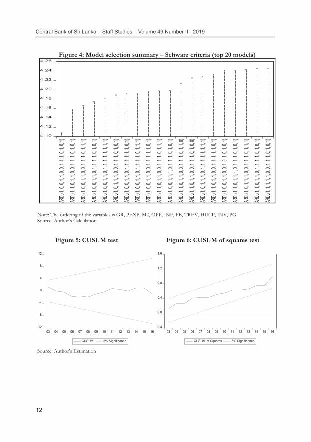
We estimated 20 ARDL models based on SIC to examine growth effects of components of public expenditure (see Figure 4). However, we selected ARDL (1, 0, 0, 1, 1, 0, 0, 1, 1, 1, 0, 1, 0, 1) model as the best model among all other models. Moreover, the stability of the estimated ARDL model was investigated using both CUSUM and CUSUMSQ methods. Since both CUSUM and CUSUMSQ statistics prevailed within the critical bounds of 5 percent level of significance, the null hypothesis of estimated coefficients of ARDL model is stable cannot be rejected. This confirms that the estimated ARDL model is stable.

As estimated ARDL model is stable, we applied ARDL Bounds tests to examine the long-run relationship among variables. Accordingly, it is found that the F-statistic value of 10.48238 exceeds the critical value of upper bounds in all three significance levels (see Table 4). Therefore, the null hypothesis of no long-run relationship can be rejected in all three significance levels and it can be concluded that all the variables move together in the long-run irrespective of their order of integration.

11

As estimated ARDL model is stable, we conducted ARDL-Bounds test to identify co-integration among variables in the model. The results of Bounds test are presented in Table 3. As calculated F-statistic is higher than upper bound critical values, the null hypothesis of no long-run (equilibrating) relationship can be rejected in all three significance level. This confirms the existence of a long-run relationship irrespective of order of integration of variables.

Table 3: ARDL bound tests for long-run relationship Test Statistic Value I(0): Lower Bound I(1): Upper Bound Asymptotic: n =1000 F-Statistic

6.78265

Significance Level Significance Level

10% 5% 1% 10% 5% 1% K

9

1.8

2.04

2.5

2.8

2.08

3.68

Source: Author’s Estimation Note: The critical value bounds are computed by stochastic simulations using 1000 replications. K represents the number of variables that we have included in the ARDL bound test.

4.2.2 ARDL model for growth effects of components of public expenditure

We estimated 20 ARDL models based on SIC to examine growth effects of components of public expenditure (see Figure 4). However, we selected ARDL (1, 0, 0, 1, 1, 0, 0, 1, 1, 1, 0, 1, 0, 1) model as the best model among all other models. Moreover, the stability of the estimated ARDL model was investigated using both CUSUM and CUSUMSQ methods. Since both CUSUM and CUSUMSQ statistics prevailed within the critical bounds of 5 percent level of significance, the null hypothesis of estimated coefficients of ARDL model is stable cannot be rejected. This confirms that the estimated ARDL model is stable.

As estimated ARDL model is stable, we applied ARDL Bounds tests to examine the long-run relationship among variables. Accordingly, it is found that the F-statistic value of 10.48238 exceeds the critical value of upper bounds in all three significance levels (see Table 4). Therefore, the null hypothesis of no long-run relationship can be rejected in all three significance levels and it can be concluded that all the variables move together in the long-run irrespective of their order of integration.

Value I(0): Lower Bound I(1): Upper Bound Asymptotic: n =1000


12

12

Figure 4: Model selection summary – Schwarz criteria (top 20 models)

4.10

4.12

4.14

4.16

4.18

4.20

4.22

4.24

4.26AR

DL(1,

0, 0, 1

, 1, 0,

0, 1, 1,

1, 0, 1

, 0, 1)

ARDL

(1, 1,

0, 1, 1,

0, 0, 1

, 1, 1,

0, 1, 0,

1)

ARDL

(1, 0,

0, 1, 1,

0, 0, 1

, 1, 1,

0, 1, 1,

1)

ARDL

(1, 0,

0, 1, 1,

0, 1, 1

, 1, 1,

0, 1, 0,

1)

ARDL

(1, 0,

0, 1, 1,

0, 1, 1

, 1, 1,

1, 1, 1,

1)

ARDL

(1, 0,

1, 1, 1,

0, 0, 1

, 1, 1,

0, 1, 0,

1)

ARDL

(1, 0,

0, 1, 1,

0, 1, 1

, 1, 1,

1, 1, 0,

1)

ARDL

(1, 0,

0, 1, 1,

0, 1, 1

, 1, 1,

0, 1, 1,

1)

ARDL

(1, 0,

0, 1, 1,

0, 0, 1

, 1, 1,

1, 1, 0,

1)

ARDL

(1, 1,

0, 1, 1,

0, 0, 1

, 1, 1,

0, 1, 1,

1)

ARDL

(1, 0,

0, 1, 1,

1, 0, 1

, 1, 1,

0, 1, 0,

1)

ARDL

(1, 1,

0, 1, 1,

0, 0, 1

, 1, 1,

0, 1, 1,

0)

ARDL

(1, 1,

0, 1, 1,

0, 0, 1

, 1, 1,

0, 1, 0,

0)

ARDL

(1, 0,

1, 1, 1,

0, 1, 1

, 1, 1,

1, 1, 1,

1)

ARDL

(1, 1,

0, 1, 1,

0, 0, 1

, 1, 1,

1, 1, 0,

1)

ARDL

(1, 0,

0, 1, 1,

0, 0, 1

, 0, 1,

0, 1, 0,

1)

ARDL

(1, 1,

0, 1, 1,

1, 0, 1

, 1, 1,

0, 1, 0,

1)

ARDL

(1, 0,

1, 1, 1,

0, 0, 1

, 1, 1,

0, 1, 1,

1)

ARDL

(1, 1,

0, 1, 1,

0, 1, 1

, 1, 1,

0, 1, 0,

1)

ARDL

(1, 1,

1, 1, 1,

0, 0, 1

, 1, 1,

0, 1, 0,

1)

Note: The ordering of the variables is GR, PEXP, M2, OPP, INF, FB, TREV, HUCP, INV, PG. Source: Author’s Calculation

Figure 5: CUSUM test Figure 6: CUSUM of squares test

Source: Author’s Estimation

-12

-8

-4

0

4

8

12

03 04 05 06 07 08 09 10 11 12 13 14 15 16

CUSUM 5% Significance

-0.4

0.0

0.4

0.8

1.2

1.6

03 04 05 06 07 08 09 10 11 12 13 14 15 16

CUSUM of Squares 5% Significance

2nd Proof17/07/2020

13


13

Table 4: ARDL bounds tests for long-run relationship Test

Statistic Value I(0): Lower Bound I(1): Upper Bound

Asymptotic: n =1000 F-Statistic 10.48238 Significance Level Significance Level 10% 5% 1% 10% 5% 1% K

13

1.76

1.98

2.41

2.77

3.04

3.61

Note: The critical value bounds are computed by stochastic simulations using 1000 replications. K represents the number of variables included in the model. Source: Author’s Estimation

4.3 The long-run impacts of public expenditure on economic growth

4.3.1 Total public expenditure

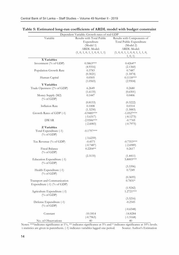
As estimated models in section 4.2.1 and 4.2.2 established a co-integration among variables, in the next step, we proceed with estimating long-run coefficients using respective ARDL specifications in two different settings. The first set of estimations, which includes total public expenditure along with other control variables, is presented in the second column of Table 5. The second set of estimation, which includes components of public expenditure, is given in the last column of Table 5.

As per model 1, total public expenditure has negative and significant impacts on growth. Holding other variables of the model constant, a one percent increase in public expenditure as a percentage of GDP is associated with approximately 0.18 percent decrease in long-term growth. This result is consistent with previous studies (Devarajan et al. 1996; Folster and Henrekson 2001), which argue that public expenditure has negative impacts on growth owing to inefficient and unproductive nature of such investments. However, the result contradicts with a previous study conducted by Herath (2010) who found positive growth effects of public expenditure for Sri Lanka. This conflicting result could be due to the inclusion of most recent data that captures recent changes in the economic structure and the usage of advanced econometrics techniques. However, given the increased public expenditure, examining the growth effects of public expenditure at disaggregated level is imperative for Sri Lanka. Therefore, a detailed analysis is conducted in the subsequent section.

13




13

1.76

1.98

2.41

2.77

3.04

3.61






13




13

1.76

1.98

2.41

2.77

3.04

3.61







14

14

Table 5: Estimated long-run coefficients of ARDL model with budget constraint Dependent Variable: Growth rates of real GDP

Variable Results with Total Public Expenditure

(Model 1) ARDL Model:

(1, 0, 1, 0, 1, 1, 0, 0, 1, 1)

Results with Components of Total Public Expenditure

(Model 2) ARDL Model:

(1, 0, 0, 1, 1, 0, 0, 1, 1, 1, 0, 1, 0, 1)

X Variables Investment (% of GDP) 0.5863*** 0.4264**

(4.9316) (2.1360) Population Growth Rate 0.3783 0.7487

(0.3021) (1.1874) Human Capital 0.0505 0.1118***

(1.0565) (2.9504) Y Variables

Trade Openness ((% of GDP) 6.2649 0.2680 (1.6135) (0.6501)

Money Supply (M2) (% of GDP)

0.1447 0.0406

(0.8153) (0.3222) Inflation Rate 0.1008 0.0314

(1.3230) (1.5883) Growth Rates of GDP (-1) -0.9485*** -1.0527***

(-5.6317) (-8.1275) DWAR -2.9306*** -0.7769

(-2.6083) (-0.7975) Z Variables

Total Expenditure (-1) (% of GDP)

-0.1797***

(-3.6259) Tax Revenue (% of GDP) -0.4571 -0.7353***

(-0.7487) (-2.6989) Fiscal Balance (% of GDP)

0.2204** 0.2617

(2.3135) (1.4411) Education Expenditure (-1)

(% of GDP) 5.8003***

(3.3396) Health Expenditure (-1)

(% of GDP) 0.7249

(0.3695) Transport and Communication Expenditure (-1) (% of GDP)

0.7831*

(1.9242) Agriculture Expenditure (-1)

(% of GDP) 1.2721***

(3.3216) Defense Expenditure (-1)

(% of GDP) -0.2545

(-0.6548) Constant -10.1814 -14.8284

(-0.7963) (-1.5168) No. of Observations 40 40

Notes: ***indicates significance at 1%, ** indicates significance at 5% and * indicates significance at 10% levels. t-statistics are given in parenthesis. (-1) indicates variables lagged one period. Source: Author’s Estimation

2nd Proof17/07/2020

15


15

4.3.2 Components of public expenditure

As evident from model 2, growth effects of total expenditure on education are found to be positive and statistically significant (see Table 5). The magnitude of growth effects of education expenditure is substantial. This result is consistent with new growth literature which strongly validates the argument of education expenditure as an essential factor in determining growth. Holding other variables constant, one percent increase in expenditure in education as a percentage of GDP is associated with an increase in average growth rate by 5.8 percent. Previous studies by Castles and Dowrick (1990) also established similar results. The positive impacts of education expenditure could be due to strong spill-over effects of investment in the education sector in raising the productivity of both human and physical capital. However, our results contradict with previous studies conducted by Barro and Sala-i-Martin (1992), Landau (1983) and Devarajan et al.(1996) that established insignificant impacts of education expenditure.

Health expenditure is considered as an investment in human capital that influences growth. However, this study found that health expenditure has a positive but insignificant impact on growth. Our finding contradicts with previous studies of Cole and Neumayer (2006) who showed positive and significant growth effects of health expenditure. Inclusion of budget constraints, which is absent in previous studies, and is limited to only Sri Lankan economy could partly explain reasons for different outcomes. To our knowledge, studies on growth effects of health expenditure are almost non-existent in the literature on Sri Lanka and therefore this study provides fresh empirical evidence.

Meanwhile, this study found growth effects of transport and communication expenditure are positive and significant. The result is consistent with previous studies conducted by Fedderke et al. (2006), who confirmed positive impacts of infrastructure on growth in South Africa. The present study also stresses that expenditure on transport and communication sector is crucial for growth. Furthermore, this study clearly establishes positive and significant growth effects of agriculture expenditure. Therefore, allocating funds towards agriculture sector would not only enhance growth but could also improve the wellbeing of rural population. Meanwhile, coefficient on defence expenditure is negative but statistically insignificant. This is consistent with previous studies such as Landau (1983) and Deger and Smith (1983). The diversion of expenditure towards unproductive sectors including defense results in a reduction of public savings and investments and thereby undermines growth. Although this study found adverse impacts of defence expenditure, some positive impacts are also justified in literature (see Frederiksen and Looney, 1983; Ram, 1986).

Looking at other variables that are considered in this study, while model 1 does not provide any evidence on growth effects of tax revenue, model 2 highlights negative and significant effects. The negative impacts of tax revenue could be identified from different channels. Increased taxation discourages both domestic and international investment and thereby adversely affects long-term growth. It also adversely affects investment in human capital and

15

4.3.2 Components of public expenditure

As evident from model 2, growth effects of total expenditure on education are found to be positive and statistically significant (see Table 5). The magnitude of growth effects of education expenditure is substantial. This result is consistent with new growth literature which strongly validates the argument of education expenditure as an essential factor in determining growth. Holding other variables constant, one percent increase in expenditure in education as a percentage of GDP is associated with an increase in average growth rate by 5.8 percent. Previous studies by Castles and Dowrick (1990) also established similar results. The positive impacts of education expenditure could be due to strong spill-over effects of investment in the education sector in raising the productivity of both human and physical capital. However, our results contradict with previous studies conducted by Barro and Sala-i-Martin (1992), Landau (1983) and Devarajan et al.(1996) that established insignificant impacts of education expenditure.

Health expenditure is considered as an investment in human capital that influences growth. However, this study found that health expenditure has a positive but insignificant impact on growth. Our finding contradicts with previous studies of Cole and Neumayer (2006) who showed positive and significant growth effects of health expenditure. Inclusion of budget constraints, which is absent in previous studies, and is limited to only Sri Lankan economy could partly explain reasons for different outcomes. To our knowledge, studies on growth effects of health expenditure are almost non-existent in the literature on Sri Lanka and therefore this study provides fresh empirical evidence.

Meanwhile, this study found growth effects of transport and communication expenditure are positive and significant. The result is consistent with previous studies conducted by Fedderke et al. (2006), who confirmed positive impacts of infrastructure on growth in South Africa. The present study also stresses that expenditure on transport and communication sector is crucial for growth. Furthermore, this study clearly establishes positive and significant growth effects of agriculture expenditure. Therefore, allocating funds towards agriculture sector would not only enhance growth but could also improve the wellbeing of rural population. Meanwhile, coefficient on defence expenditure is negative but statistically insignificant. This is consistent with previous studies such as Landau (1983) and Deger and Smith (1983). The diversion of expenditure towards unproductive sectors including defense results in a reduction of public savings and investments and thereby undermines growth. Although this study found adverse impacts of defence expenditure, some positive impacts are also justified in literature (see Frederiksen and Looney, 1983; Ram, 1986).

Looking at other variables that are considered in this study, while model 1 does not provide any evidence on growth effects of tax revenue, model 2 highlights negative and significant effects. The negative impacts of tax revenue could be identified from different channels. Increased taxation discourages both domestic and international investment and thereby adversely affects long-term growth. It also adversely affects investment in human capital and


1616

entrepreneurial activities. However, investigating growth effects of components of tax revenue is beyond the scope of this study. The budget surplus has significant positive impacts on growth in both models. Holding other variables constant, one percent increase in fiscal surplus as a share of GDP is associated with an increase in annual growth rate by an average of 0.22 and 0.26 percent in model 1 and 2 respectively. This highlights that controlling fiscal deficit is vital to enhance long-term growth.

Looking at growth effects of non-fiscal variables, the study found that investment played a crucial role in stimulating growth, which is consistent with neoclassical growth theory. Several previous studies including a study by Levine and Renelt (1992) also acknowledge investment as important determinants of growth. Holding other variables constant, one percent increases in total investment as a percentage of GDP is associated with an increase in growth rate by 0.6 percent in model 1 and 0.4 percent in model 2. This necessitates the creation of a conducive environment in Sri Lanka to attract both domestic and global investment. Human capital is found to have a positive impact on growth in both models though significance can be observed only in model 2. While inflation, population growth, money supply and trade openness accord well with theoretical predictions, they are turn out to be insignificant in both models. It is evident that growth can be accounted for by its own innovations. The study also confirmed that civil war had negatively affected growth in both models though the significance could be identified only in model 1.

4.4 Estimation of ARDL Error Correction Model (ECM) As the Bounds test established a long-run co-integration among variables, we will use ECM of ARDL to estimate short-run dynamics among the variables. The error correction term is negative and significant in both models. This shows a high level of speed of adjustment to long-run equilibrium following a short-run shock (see Table 6). About 34.41 percent and 52.70 percent of disequilibrium from previous year’s short-run shocks converges back to long-run equilibrium each year in model 1 and 2.

Although signs of short-run coefficients of total public expenditure are in line with Keynesian theoretical outpourings, its impact on growth is insignificant. It is found that total expenditure on education and agriculture, has a similar impact in the short-run too but with different magnitudes. However, the transport and communication expenditure that exhibited positive and significant impacts on long-run growth do not provide any evidence in the short-run. Growth effects of health expenditure is insignificant in the short-run as well. Similar to long-term results, growth effects of fiscal balance are positive though impact is significant only in model 1. However, the degree of impacts is much lower in the short-run compared to the long-run. This result strengthens the argument in favour of rapidly implementing effective policies for deficit reduction in Sri Lanka.

16

entrepreneurial activities. However, investigating growth effects of components of tax revenue is beyond the scope of this study. The budget surplus has significant positive impacts on growth in both models. Holding other variables constant, one percent increase in fiscal surplus as a share of GDP is associated with an increase in annual growth rate by an average of 0.22 and 0.26 percent in model 1 and 2 respectively. This highlights that controlling fiscal deficit is vital to enhance long-term growth.

Looking at growth effects of non-fiscal variables, the study found that investment played a crucial role in stimulating growth, which is consistent with neoclassical growth theory. Several previous studies including a study by Levine and Renelt (1992) also acknowledge investment as important determinants of growth. Holding other variables constant, one percent increases in total investment as a percentage of GDP is associated with an increase in growth rate by 0.6 percent in model 1 and 0.4 percent in model 2. This necessitates the creation of a conducive environment in Sri Lanka to attract both domestic and global investment. Human capital is found to have a positive impact on growth in both models though significance can be observed only in model 2. While inflation, population growth, money supply and trade openness accord well with theoretical predictions, they are turn out to be insignificant in both models. It is evident that growth can be accounted for by its own innovations. The study also confirmed that civil war had negatively affected growth in both models though the significance could be identified only in model 1.

4.4 Estimation of ARDL Error Correction Model (ECM) As the Bounds test established a long-run co-integration among variables, we will use ECM of ARDL to estimate short-run dynamics among the variables. The error correction term is negative and significant in both models. This shows a high level of speed of adjustment to long-run equilibrium following a short-run shock (see Table 6). About 34.41 percent and 52.70 percent of disequilibrium from previous year’s short-run shocks converges back to long-run equilibrium each year in model 1 and 2.


2nd Proof17/07/2020

17


17

Table 6: ARDL Error Correction Model of the growth equation Dependent Variable: Growth rates of real GDP

Variable Results with Total Public Expenditure

[ARDL (1, 0, 1, 0, 1, 1, 0, 0, 1, 1)]

Results with Components of Total Public Expenditure

[ARDL (1, 0, 0, 1, 1, 0, 0, 1, 1, 1, 0, 1, 0, 1)]

X Variables D(INV) 0.3441*** 0.5841***

(3.9959) (5.6434) D(PG) 0.3783 0.0314

(0.8623) (1.5883) D(HUCP) 0.1039

(1.2609) Y Variables

D(M2) -0.6560*** (5.3981)

D(INF) -0.0939*** -0.6632* (-2.9265) (-1.9409)

WRDUM -2.9306*** -7.7612*** (-8.2899) (-16.4002)

Z Variables D(PEXP(-1)) 0.0020

(0.0839) D(FB) 0.6889*** 0.5593***

(7.6513) (10.5940) D(EDU) 3.7185***

(7.6721) D(HTH) 0.0049

(0.0772) D(AGR) 0.2076**

(1.9636) ECM (-1) -0.3441*** -0.5270***

(-3.9959) (-8.5970) R-squared 0.8307 0.9274 Adj. R2 0.7989 0.9079

Durbin-Watson stat 1.9792 2.04265 Notes: ***indicates significance at 1%, ** indicates significance at 5% and * indicates significance at 10% levels. Source: Author’s Calculation



1818

Although growth effects of inflation are insignificant in the long-run, they have a negative and significant impact in the short-run. The main policy message is that reducing inflation by 1 percent could raise growth by 0.66 percent. This provides strong evidence to support the view of low inflation to stimulate short-term growth. Moreover, investigating channels through which inflation affects growth is essential, but it is beyond the scope of this study. Growth effects of investment exhibit positive and significant results in both models, which is consistent with long-run results. Although long-run growth effects of money supply are consistent with theoretical prediction, the study shows that money supply has significantly affected growth in the short-run. It is also evident that the civil war undermined economic growth in the short-run as well. The short-run impacts of all other variables are insignificant though they had expected sign in both models.

5. Conclusion

This study provides new empirical understanding on growth effects of public expenditure at both aggregate and disaggregate levels for Sri Lanka considering the full implication of government budget constraints. The present study found that the growth effects of public expenditure vary at the disaggregated level. The growth effects of total expenditure on education and transport and communication were found to be positive and statistically significant, while health, agriculture and defense expenditure were found to be statistically insignificant. Looking at growth effects of non-fiscal variables, the study found that investment and human capital played a crucial role in stimulating growth in Sri Lanka. Given the positive and significant growth effects of expenditure on education, agriculture, transport and communication and negative but insignificant impacts of defense expenditure, this study suggests that reforming public expenditure in particular in favor of human capital development could stimulate long-term growth in Sri Lanka. As it is found that the tax revenue has adversely affected economic growth, the present study recommends that controlling possible detrimental impacts of taxation is vital to enhance growth. Given the positive growth effects of fiscal surplus, this study recommends that controlling fiscal deficit is paramount for sustainable growth. Based on the findings, this study proposes several lines of further investigation and some possible extensions to the research content of this study. As growth effects of public expenditure at disaggregated levels have shown mixed results, in-depth studies focusing on disaggregated components even within these categories should be conducted. Although the present study showed valuable insights on growth effects of tax revenue, it is necessary to address potential growth implications arising from taxation at disaggregated levels.

2nd Proof17/07/2020

19


19

References

Afonso, A. and Furceri, D. 2008. “Government Size, Composition, Volatility and Economic Growth”. Working Paper Series 849, European Central Bank.

Avila, D. R. and Straugh, R. 2003. “Public Finances and Long-term Growth in Europe – Evidence from a Panel Data Analysis”, Working Paper Series. 246, European Central Banking.

Barro, R. 1990. “Government Spending in a Simple Model of Endogenous Growth”. Journal of Political Economy, 98(1), 103–117.

Barro, R. and Sala-i-Martin, X. 1992. “Public Finance in Models of Economic Growth”. Review of Economic Studies, 59, 645-661.

Bose, N., Haque, M. E. and Osborn, D. R. 2007. “Public Expenditure and Economic Growth: A Disaggregated Analysis for Developing Countries”. The Manchester School. 75 (5): 533-556.

Castles, F. G. and Dowrick, S. 1990. “Impact of Government Spending Levels on Medium Term Economic Growth in the OECD, 1960–1985”. Journal of Theoretical Policies. 2, 173–204.

Central Bank of Sri Lanka, Annual Reports, Various Years.

Cole, M. A. and Neumayer, E. 2006. “The Impact of Poor Health on Total Factor Productivity”. Journal of Development Studies, 42 (6), 918–38.

Cooray, A. 2009. “Government Expenditure, Governance and Economic Growth”. Comparative Economic Studies, 51 (3), 401-418.

Deger, S. and Smith, R. 1983. “Military Expenditure and Growth in Less Developed Countries”. Journal of Conflict Resolution, 27 (2), 335-353.

Devarajan, S., Swaroop, V. and Zou, H. F. 1996. “The Composition of Public Expenditure and Economic Growth”. Journal of Monetary Economics. 37 (2), 313–344.

Dilrukshini, W. A. 2004. “Expenditure and Economic Growth in Sri Lanka: Co-integration Analysis and Causality Testing”. Staff Studies, 34, 51–68.

Easterly, W. and Rebelo, S. 1993. “Fiscal Policy and Economic Growth: An Empirical Investigation”. Journal of Monetary Economics, 32, 417-458.

Fedderke, J., Perkins, P. and Luiz, J. 2006. “Infrastructural Investment in Long-run Economic Growth: South Africa 1875- 2001”. World Development, 34(6), 1037-1059.


2020

Folster, S. and Henrekson, M. 2001. “Growth Effects of Government Expenditure and Taxation in rich Countries”. European Journal of Political Economy. 45, 1501–1520.

Frederiksen, P. C. and Robert E. Looney. 1983. “Defense Expenditures and Economic Growth in Developing Countries: Some Further Evidence.” Journal of Economic Development. 7, 113–26.

Grossman, G. and Helpman, E. 1991. Quality Ladders in the Theory of Growth. The Review of Economic Studies, 58(1), 43-61.

Herath, S. 2010. “Size of the Government and Economic Growth: An Empirical Study of Sri Lanka”. SRE Discussion Papers 2010/05, WU Vienna University of Economics and Business, Austria.

Jayawickrama, A. (2004). “Fiscal Policy Sustainability: Evidence from Sri Lanka”. Sri Lanka Economic Journal 5(1): 55-74.

Johansen, S. and Juselius, K. 1990. “Maximum Likelihood and Inference on Cointegration with Applications to the Demand for Money”. Oxford Bulletin of Economics and Statistics, 52(3), 169-210.

Keynes, J. M. 1936. “General Theory of Employment, Interest and Money”. Harcourt, Brace and Co, New York, NY, USA.

Komain, J. and Brahmasrene, T. 2007. “Relationship between Government Expenditures and Economic Growth in Thailand.” Journal of Economics and Economic Education Research. 8 (1), 93–102.

Kremers J.J.M., Ericsson N. R., and Dolado, J. J. 1992. “The Power of Cointegration Tests.” Oxford Bulletin of Economics and Statistics, 54, 325–348.

Lahirushan, K. P. K. S. and Gunasekara, W. G. V. 2015. “The Impact of Government Expenditure on Economic Growth: A Study of Asian Countries”, International Journal of Humanities and Social Sciences. 9(9). 3152-3160.

Landau, D. 1983. “Government Expenditure and Economic Growth: A Cross-Country Study”. Southern Economic Journal, 49(3), 783-792.

Levine, Ross, and David Renelt. 1992. "A Sensitivity Analysis of Cross-Country Growth Regressions," American Economic Review, LXXXII, 942-63.

Lucas, R. E. 1988. “On the Mechanics of Economic Development”. Journal of Monetary Economics, 22, 3-42.

Pesaran, M. H, Pesaran, B. 1997. “Working with Microfit 4.0: Interactive Econometric Analysis”, Oxford University Press: Oxford.

20















Kesavarajah, M., 2012. Wagner’s Law in Sri Lanka: An Econometric Analysis, International Scholarly Research Network, Vol. Article ID 573826, pp. 1-9.

Kesavarajah, M., 2017. Growth Effects of Fiscal Deficits in Sri Lanka. Staff Studies, 47(1), pp.47–68.

2nd Proof17/07/2020

21


20















21

Ram, R. 1986. “Government size and Economic Growth: A New Framework and some evidence from Cross-section and Time-series data.” American Economic Review, 76(1), 191-203.

Ramayandi, A. 2003. “Economic Growth and Government Size in Indonesia: Some Lessons for the Local Authorities”. Working Papers in Economics and Development Studies, Padjadjaran University.

Ranjan, K. D. and Sharma, C. 2008. “Government Expenditure and Economic Growth: Evidence from India”. The ICFAI University Journal of Public Finance, 6 (3), 60-69.

Ravinthirakumaran, N. and Kesavarajah, M. (2011), "The Impact of Government Expenditure on Economic Growth in Sri Lanka: An Econometric Analysis" in Proceedings of the 8th International Conference on Business Management, Faculty of Management Studies and Commerce, University of Sri Jayewardenepura, Nugegoda, Sri Lanka.

Tanzi, V. and H. Zee. 1997. “Fiscal Policy and Long-run Growth”, IMF Staff Papers. 44 (2), 179-209.

Wagner, A. 1883. “Three Extracts on Public Finance”. in R.A. Musgrave and A.T. Peacock (eds) (1958), “Classics in the Theory of Public Finance”, London: Macmillan.

World Bank. 2018. World Development Indicators. Washington, DC: World Bank.


2222

Appendices

A.1 Information on data

Figure A1: Behaviour of the variables

Note: The detailed descriptions of the variables are given in Table A1

-4

0

4

8

12

80 85 90 95 00 05 10 15

GR

120

140

160

180

200

80 85 90 95 00 05 10 15

HUCP

0

5

10

15

20

25

30

80 85 90 95 00 05 10 15

INF

20

25

30

35

40

45

80 85 90 95 00 05 10 15

M2

.3

.4

.5

.6

.7

.8

80 85 90 95 00 05 10 15

OPP

15

20

25

30

35

40

45

80 85 90 95 00 05 10 15

PEXP

0.0

0.5

1.0

1.5

2.0

2.5

80 85 90 95 00 05 10 15

PG

8

12

16

20

24

28

80 85 90 95 00 05 10 15

TREV

0

2

4

6

8

10

12

80 85 90 95 00 05 10 15

AGR

0

5

10

15

20

25

80 85 90 95 00 05 10 15

CPEXP

12

16

20

24

28

80 85 90 95 00 05 10 15

CREXP

0

1

2

3

4

5

6

80 85 90 95 00 05 10 15

DEF

-20

-16

-12

-8

-4

80 85 90 95 00 05 10 15

FD

12

16

20

24

28

32

80 85 90 95 00 05 10 15

INV

1.0

1.2

1.4

1.6

1.8

2.0

2.2

80 85 90 95 00 05 10 15

HTH

0

1

2

3

4

5

6

80 85 90 95 00 05 10 15

TRC

1.5

2.0

2.5

3.0

3.5

80 85 90 95 00 05 10 15

EDU

0

1

2

80 85 90 95 00 05 10 15

WRDUM

2nd Proof17/07/2020

23


23

Table A1: Definition of the variables and data sources Variable Definition of Variables Data Source GDP Data gr Growth rate of GDP World Bank Development

Indicators Conditioning Variables (X) inv Gross fixed capital formation (% of GDP) World Bank Development

Indicators pg Population growth rate DCS hucp Human capital (primary, secondary and tertiary school

enrolment ratio) Barro and Lee (1994)

Control Variables (Y) opp Exports and imports share of GDP (trade openness) CBSL m2 Broad Money (M2) (% of GDP) CBSL inf Inflation rate as the percentage change of CPI DCS gr(-1) One period lag of growth rate of GDP CBSL wrdum Dummy variable to capture civil war

(1 for 1983-2009 and 0 for otherwise)

Fiscal Variables (Z) pexp Public expenditure (% of GDP) CBSL pexp(-1) One period lag of public expenditure

(% of GDP) CBSL

rev Government revenue (% of GDP) CBSL fb Fiscal Balance (surplus/deficit) (% of GDP) CBSL Components of Government Expenditure

edu Government expenditure in education (% of GDP) CBSL hth Government expenditure in health expenditure

(% of GDP) CBSL

trc Government expenditure in Transport and Communication (% of GDP)

CBSL

agr Government expenditure in Agriculture and Irrigation (% of GDP)

CBSL

def Government expenditure in Defense (% of GDP) CBSL Components of Government Revenue trev Tax revenue (% of GDP) CBSL

Note: CBSL-Central Bank of Sri Lanka, DCS-Department of Census and Statistics of Sri Lanka

A.2 Construction of human capital variable

Literatures including Easterly and Rebelo (1993) and Barro and Sala-i-Martin (1999) uses enrolment rates for human capital variable. However, in this study, we follow Bose et al. (2007) to construct the initial human capital variable. In this study, the human capital variable is a weighted sum of initial enrolment ratios in primary, secondary and higher education. The weights are 1 for primary school, 2 for secondary school and 3 for higher education. Weights are approximations to the relative values of three types of education. The construction of the human capital variable is based on the Barro and Lee (2000) data source.


24

24

Table A2: Descriptive statistics of the variables

Variable Obs Mean Median Min Max Std. Dev.

gr 40 5.1089 5.0999 -1.5454 9.1446 1.9028

pg 40 1.0978 1.1750 -2.2400 2.3500 0.8036

opp 40 0.5782 0.5958 0.3638 0.7741 0.1192

hucp 40 8.8883 9.3500 6.7200 10.3100 1.3528

inv 40 24.7176 24.7965 13.8298 31.3331 3.2970

inf 40 10.2500 9.6000 1.2000 26.1000 5.6426

m2 40 31.1175 30.9000 23.9000 40.7000 2.8616

pexp 40 27.6475 27.1000 17.3000 42.7000 6.1954

fb 40 -8.6025 -8.1000 -19.2000 -4.5000 2.7945

trev 40 15.5325 15.0500 10.1000 24.2000 3.0780

agr 40 2.1499 1.2802 0.6945 10.3932 2.2363

def 40 2.4672 2.4729 0.4897 5.2692 1.2292

edu 40 2.4252 2.4886 1.5597 3.2320 0.4166

hlth 40 1.5174 1.5370 1.1337 2.0169 0.2395

trc 40 2.4758 2.4027 0.7229 5.2158 0.8352

Note: The detailed descriptions of the variables are given in Table A1 in Appendix

Figure A2: Trends in public expenditure: disaggregated analysis

Source: Central Bank of Sri Lanka

0.0

5.0

10.0

15.0

20.0

25.0

30.0

35.0

40.0

45.0

0.0

2.0

4.0

6.0

8.0

10.0

12.0

1977

19

79

1981

19

83

1985

19

87

1989

19

91

1993

19

95

1997

19

99

2001

20

03

2005

20

07

2009

20

11

2013

20

15

Perc

ent

Perc

ent

Defence Education Health Agriculture Transport & Communication Total Expenditure (RHS)

2nd Proof17/07/2020

25


25

Table A3: Selection of optimal lag length

Lag LogL LR FPE AIC SIC HQ

0

-659.7271 NA 59.4367 35.3014 35.7755 35.4701 1 -359.8285 410.3875* 0.0062 25.8857 31.5742* 27.9096 2 -183.9458 138.8548 0.0022* 22.9972* 33.9000 26.8763*

Note: * indicates lag order selected by the criterion, LR: sequential modified LR test statistic, FPE: Final prediction error, AIC: Akaike information criterion, SIC: Schwarz information criterion, HQ: Hannan-Quinn information criterion (each test at 5% significance level)

Source: Author’s Calculation

A.3 Testing for structural breaks in public expenditure and economic growth

As our sample involves the time period around the financial crisis of 2008 and the end of the civil war in 2009, we examined structural breaks in public expenditure (PEXP) and economic growth (GR). This study uses a global maximiser test introduced by Bai and Perron (2003) to determine the years of any structural breaks.

Table A4: Identification of structural break for public expenditure

Dependent Variable: PEXP Method: Least Squares with Breaks Sample (adjusted): 1981 2016 Break type: Bai-Perron tests of L+1 vs. L sequentially determined breaks Break selection: Trimming 0.15, Max. breaks 5, Sig. level 0.05 No breakpoints selected

Variable Coefficient Std. Error t-Statistic Prob.

PEXP(-1) 0.560567 0.155598 3.602653 0.0011 PEXP(-2) 0.119634 0.174111 0.687113 0.4971 PEXP(-3) -0.002657 0.149258 -0.017801 0.9859 PEXP(-4) 0.233271 0.108040 2.159114 0.0387 Non-Breaking Variables

C 1.446762 1.785148 0.810444 0.4239 R-squared 0.877580 Mean dependent var 26.69167 Adjusted R-squared 0.861784 S.D. dependent var 5.219654 S.E. of regression 1.940532 Akaike info criterion 4.292048 Sum squared resid 116.7356 Schwarz criterion 4.511981 Log likelihood -72.25686 Hannan-Quinn criter. 4.368810 F-statistic 55.55670 Durbin-Watson stat 1.892250 Prob(F-statistic) 0.000000



26

26

Table A5: Identification of structural break for economic growth rate

Dependent Variable: GR Method: Least Squares with Breaks Sample (adjusted): 1981 2016 Break type: Bai-Perron tests of L+1 vs. L sequentially determined breaks Break selection: Trimming 0.15, Max. breaks 5, Sig. level 0.05 No breakpoints selected Variable Coefficient Std. Error t-Statistic Prob. GR(-1) 0.225703 0.179749 1.255657 0.2186 GR(-2) 0.043694 0.183342 0.238320 0.8132 GR(-3) -0.031467 0.183389 -0.171587 0.8649 GR(-4) -0.017750 0.180679 -0.098240 0.9224

Non-Breaking Variables C 3.921429 1.537254 2.550932 0.0159 R-squared 0.057263 Mean dependent var 5.037537 Adjusted R-squared -0.064381 S.D. dependent var 1.989329 S.E. of regression 2.052367 Akaike info criterion 4.404111 Sum squared resid 130.5786 Schwarz criterion 4.624044 Log likelihood -74.27400 Hannan-Quinn criter. 4.480874 F-statistic 0.470743 Durbin-Watson stat 1.998211 Prob(F-statistic) 0.756761


2nd Proof17/07/2020

27

27

Real Wages, Inflation and Labour Productivity: Evidence from the Public and Private Sectors in Sri Lanka

Rohini D. Liyanage1

Abstrac t

Productivity as a measure of efficiency, how productively a nation produces its goods and services using its limited resources, a measure of competitiveness among the nation in the global world, has been a current research interest of many. The main objective of this study is to examine and analyse the relationships between real wages, inflation and labour productivity in Sri Lanka during the period from 2006 to 2019 using quarterly, secondary and seasonally adjusted data. Identifying the factors affecting labour productivity and determining the causal relationship among variables are secondary objectives. The Ordinary Least Square (OLS) and Vector Auto Regression (VAR) models are employed to determine the static and dynamic relationship among Labour productivity (LPDCT), Colombo Consumer Price Index (CCPI), Real Wages in Government Sector (RWGSEC), Real Wages in Private Sector (RWPSEC) and Real Wages in Informal Private Sector (RWIPSEC). Accordingly, in the short run, a negative dynamic relationship between inflation and labour productivity, and a positive relationship between real wages of all sectors and labour productivity are identified. As per the results of FEVD, DLPDCT is a strongly endogenous variable while other variables are least exogenous. Real wages of Private Sector and Real Wages of Informal Private Sector employees’ contributions to labour productivity are significant compared to the Real Wages of Government Sector employees as per the analysis of the sample period. Results suggest that economic growth stimulating policies, and that well-managed lower level inflation, increasing Real Wages of PSEC employees, encourage PSEC by facilitating initial requirements, infrastructure, innovations, research and development to enhance labour productivity. Allocating and assigning more work to government sector employees can be recommended as a measure to further enhance labour productivity in Sri Lanka. One directional causality exists from DLPDCT towards DLCCPI. Further, inflation Granger caused real wages in Private Sector employees as per the Granger Causality Block Erogeneity test during the period studied.

Key Words : Labour Productivity, Inflation, Real Wages, VAR, Sri Lanka

1 The author is currently serving as a Senior Assistant Director of the Payments and Settlements Department. Corresponding email: [email protected] She would like to thank Mr A.T. Sooriyaarachchi and Ms. B.N.K. Fernando for their support. Further, the author is thankful to the anonymous reviewers for their comments and advice. The views presented in the paper are those of the author and do not necessarily indicate the views of the Central Bank of Sri Lanka

.

Abstract

Key Words: Labour Productivity, Inflation, Real Wages, VAR, Sri Lanka


28

28

1. Introduction

Productivity can be identified as a measure of efficiency of production, and a measure for competitiveness among nations. Therefore, the factors affecting productivity are also of paramount importance in order to identify the relationship and make recommendations to enhance productivity, as well as to achieve higher economic growth and other long-term objectives of any economy. "Productivity isn't everything, but in the long run it is almost everything. A country's ability to improve its standard of living over time depends almost entirely on its ability to raise its output per worker" (Krugman). It provides a basis for consumption, savings, investments, poverty reduction and is a vital factor of international competitiveness. Hence, productivity improvement is a substantial issue for many countries. Real wages and inflations can be identified as key determinants of labour productivity as per theoretical and empirical literature. Labour productivity is defined as the output per unit of labour input which is considered a measure of efficiency and expressed as a ratio of GDP. Wages can be identified as return to the labour compensation to the employer. Real wages are wages adjusted for inflation, measured by the consumer price index and providing a guide for the changes to the cost of living. Inflation can be identified as a continuous increase of the general price level of a country as measured by consumer price indices.

As per the Production function, production is a function of factors of production, namely labour and capital. In the short run, only labour can be changed while other factors change only in the long run. Other factors include capital, technological change and population growth. Wages are monetary compensation paid by a firm for the commitment of labour for the workers. Therefore, wages are the primary source of income and expenditure in a household. Real wages can be defined as wages adjusted for inflation, or the purchasing power of nominal wages that workers are interested in. Higher inflation leads to lower real wages due to erosion of the purchasing power of the nominal wages. Therefore, both wages and inflation are concerns in labour market related issues. Efficiency wages, average wages and minimum wages are found among labour market concepts. Countries have convergence in minimum wages to ensure the basic requirements of workers. (Shapiro and Stiglitz) found that the Efficiency wage theory is based on the idea that increasing wages can increase labour productivity. Efficiency wages can be identified as wages above the equilibrium level of the market, and there are reasons for existing efficiency wages in the market. Risk of the opportunity cost of job loss is higher and thus workers tend to work more efficiently. When labour cost is higher, firms change factor inputs by substituting capital for labour which causes increase in the Marginal Productivity of Labour (MPL). As per the Neo-classical theory, wage determination is based on the marginal productivity of labour. As per empirical evidence, the relationship between real wages and productivity are positive (Narayan and Smyth; Wakeford ; Strauss and Wohar; Alexander; Hall). Such findings are supported by the efficiency wage hypothesis and a mix of factor inputs from labour to capital. (Gordon) explains that factor

As per the Production function, production is a function of factors of production, namely labour and capital. In the short run, only labour can be changed while other factors change only in the long run. Other factors include capital, technological change and population growth. Wages are monetary compensation paid by a firm for the commitment of labour for the workers. Therefore, wages are the primary source of income and expenditure in a household. Real wages can be defined as wages adjusted for inflation, or the purchasing power of nominal wages that workers are interested in. Higher inflation leads to lower real wages due to erosion of the purchasing power of the nominal wages. Therefore, both wages and inflation are concerns in labour market related issues. Efficiency wages, average wages and minimum wages are found among labour market concepts. Countries have convergence in minimum wages to ensure the basic requirements of workers. (Shapiro and Stiglitz) found that the Efficiency wage theory is based on the idea that increasing wages can increase labour productivity. Efficiency wages can be identified as wages above the equilibrium level of the market, and there are reasons for existing efficiency wages in the market. Risk of the opportunity cost of job loss is higher and thus workers tend to work more efficiently. When labour cost is higher, firms change factor inputs by substituting capital for labour which causes increase in the Marginal Productivity of Labour (MPL). As per the Neo-classical theory, wage determination is based on the marginal productivity of labour. As per empirical evidence, the relationship between real wages and productivity are positive (Narayan and Smyth; Wakeford; Strauss and Wohar; Alexander; Hall). Such findings are supported by the efficiency wage hypothesis and a mix of factor inputs from labour to capital. (Gordon) explains that factor

29


29

substitution from labour to capital in response to inexorable/unstoppable increases in real wages has been at the heart of the economic growth process for centuries.

Inflation is a short-term objective of the monetary authorities of a country. In stabilization policies, which include fiscal and monetary policy, more attention has been paid to keeping a lower level inflation to achieve long term objectives of an economy. Some developed countries have converged to maintain a lower level of inflation that has defined below 2 per cent. Inflation negatively impacts productivity due to the impact of worker purchasing power, motivation and effort. Further, inflation impacts investment plans of firms, capital depreciation rates and substitution of factor inputs that is capital for labour. An inflation and real wages related study by (Hendry) concludes that inflation responds to many parts of an economy including labour cost and labour market. A negative relationship between inflation and labour productivity has been established in the majority of empirical analysis. (Freeman and Yerger "Does Inflation Lower Productivity? Time Series Evidence on the Impact of Inflation on Labor Productivity in 12 Oecd Nations") examine whether there is an empirical support to reduce already low rates of inflation to increase labour productivity growth and economic growth. Findings do not support the view that further reductions in inflation from already low single-digit levels would have a positive impact on labour productivity growth for major industrial countries. Therefore, it is a well-established fact that there must be a stable lower level inflation rate to stimulate economic activity and growth while a higher level of inflation is harmful to encourage economic activities. Several arguments point out that this inverse relationship is spurious due to cyclical movements of the variables.

In Sri Lanka, labour productivity has performed well compared to the other countries of the region. Being a competitive nation is important in the globalized world among its peer countries. Higher economic growth is a primary factor of increasing productivity. Countries with a higher economic growth enhance their productivity, living standards and competitiveness. Economic growth in Sri Lanka has been limited to around 5 per cent for the last two decades. Inflation also has been managed at mid-single digits level after the end of civil war in 2009. Wages of government and private sector employees increase with the bargaining powers of trade unions periodically, and for government sector employees, the COLA allowance is additionally annexed to the wages that link to the inflation. As per the Central Bank of Sri Lanka (Central Bank of Sri Lanka Annual Reports 2018; Central Bank of Sri Lanka Annual Report 2019) real wage erosion was prominent in both government and private sector employees. This might have resulted in deteriorating living standards, consumption and exposing employees to the poverty margin since wages are their primary source of expenditure. Lower real wages lead to lower labour productivity even with easing inflation. Inflation keeps at a lower level in Sri Lanka, and economic growth is slowly improving while real wages are improving in the government and informal private sectors. With these recent developments, it is required to examine whether there is a possibility to stimulate economic growth and enhance productivity to facilitate higher standard of living, competitiveness and achieve other


30

30

long-term objectives. Further, according to the (Asian Development Bank, International Labour Organisation and Regional Office for Labour the Pacific) Sri Lanka has entered a demographic transition characterized by lower birth and death rates. This causes the working-age population to decline with an ageing of society and the rising age dependency ratio. To sustain the expenses, a higher growth rate is to be achieved to cushion the requirements of pensions, health and other expenses. Further, Sri Lanka was categorized as an upper middle-income country based on the per capita gross national income in 2017, while later the category was downgraded to a lower middle-income country in 2020 considering revisions to national accounting methods and adjustments to keep income classification thresholds fixed in real time. However, it takes a long time to reach the upper level income status compared to other emerging market economies. Now the challenge of the Middle-Income Trap (MIT) must be overcome through efficiency-based productivity which comes by together with technology and innovations. In this regard, (Pruchnik and Zowczak) point out that being stuck in MIT could be led by decrease of productivity due to factors like less economic diversification, the inelastic and inefficient labour market, inefficient financial market, outdated infrastructure facilities, inefficient institutions and less innovations. As per the above categorization, Sri Lanka belongs to the lowest level of economic diversification and inefficient labour market. Therefore, in order to overcome this challenge, the next level would rely on efficiency driven productivity growth. Therefore, in all these scenarios, an increase in labour productivity is essential to sustain economic growth and thereby achieve a higher standard of living, the wellbeing of the nation and to maintain the economy’s competitiveness.

Studies have covered mostly developed countries such as the USA, the UK, European countries, Australia, Japan, Korea and Malaysia. Further, Studies has been limited to capture the real wages of the manufacturing and mining sector while contributions of other sectors are also substantially high in the economy. From the economic viewpoint, contributions of agriculture, industry and service sectors change when economic transits happen. Further, Panel data analysis techniques have been used to examine problems related to macro-economic variables that are different country-wise. In some studies, small sample and annual data have been employed while data frequency is monthly or quarterly for the macroeconomic variables. More attention is paid to the relationship between inflation and labour productivity and conclude with endless arguments that the relationship between inflation and productivity is spurious due to variables are not integrated in same order and cyclical movements of the variables. Further, no studies have been conducted on inflation, real wages and labour productivity in the case of Sri Lanka. Therefore, with the existing gap in the literature on the relevant field, this study tries to fill the vacuum in literature related to the relationship among inflation, real wages and labour productivity covering both government and private sectors using quarterly, secondary data. The direction of causality is also considered, which has been covered in many studies but has ended up in different findings based on the data. Therefore, this study contributes to fill the existing gap in literature and methodology, and makes policy

31


31

level recommendations in order to improve labour productivity subject to managing inflation and improving real wages and the wellbeing of the society. The aim of this study is to analyse the relationship among real wages, inflation and labour productivity of the public and private sectors in Sri Lanka from 2006 to 2019. Finally, the causality among inflation, real wages and labour productivity are examined to better predict variables using lag values of others.

The remainder of this paper is structured as follows: section 2 is allocated for conceptual, theoretical and empirical literature and critical reviews related to inflation, real wages and labour productivity and thereby a research gap is identified, and the importance of contribution in terms of theory, methodology and policy related recommendations are pointed out. Methodological aspects of the research are discussed in section 3 covering the economic approach, conceptual framework, analytical methods and data collection methods, sources etc. Data presentation and analysis are done in section 4. Finally, section 5 is devoted to the summary of findings, theoretical relevance, conclusions, inferences and policy recommendations.


2.1 Theory and empirical literature There are theories of inflation, real wages and productivity that are separately described in literature. Empirical literature on the topics can be categorized into three as the relationship between inflation and labour productivity, real wages and labour productivity, and inflation real wages and labour productivity, and is reviewed below.

2.2 Inflation and productivity Interest on inflation and productivity has been a growing concern with the stabilization policy conditions set under the fiscal and monetary discipline. Economists’ argument on inflation and productivity can be identified as inflation having a negative impact on productivity through price signalling to economic agents and sectors. Firstly, inflation impacts worker purchasing power, a mix of factor inputs and to the investment’s plans. Worker purchasing power is from the labour supply side factor and the other two are from a production point of view. (Feldstein) concludes that given the existing tax structure, inflation lowers the real return on capital. A number of studies have been conducted related to inflation and productivity. Research covers the USA and European countries with panel data analysis, and econometric techniques are used for annual or quarterly data while stationary test and cointegration test in Johansen methodology are followed. Findings of empirical literature are in line with theory and give somewhat different views from theoretical concepts. Accordingly, many studies (Clark; Bårdsen, Hurn and McHugh; Buck and Fitzroy; Christopoulos and Tsionas; De Gregorio; Narayan and Smyth; Smyth) conclude that there is a negative relationship between inflation and productivity.(Kim, Lim and Park) suggest that productivity


32

32

inflation nexus became stronger in Korea due to Asian financial crisis. One study from the few studies conclude with mixed findings. (Sbordone and Kuttner) conclude that there is a negative relationship between inflation and labour productivity. Further, they show that it is difficult to conclude as higher inflation causes productivity to fail. This conclusion is made regarding the US, covering the period of 1949-94 post-war evidence. (Cameron, Hum and Simpson) in the study of Stylized facts and stylized illusions, inflation and productivity revisit covering Canada, the USA, the UK and West Germany. They conclude that there is no evidence for any connection between inflation and productivity growth in the long run while there is a strong connection between inflation and productivity growth in the short run, and that it depends entirely on the cointegration and stationary properties of the variables.

(Freeman and Yerger "Inflation and Multifactor Productivity Growth: A Response to Smyth") conclude that the impact of inflation on multifactor productivity growth is so minor that it did not show up as statistically significant in the analysis. Moreover, (Freeman and Yerger "Does Inflation Lower Productivity? Time Series Evidence on the Impact of Inflation on Labor Productivity in 12 OECD Nations") show that there is no evidence of a consistent relationship between inflation and productivity growth with regard to either sign or magnitude. Therefore, study does not support to further reduction of low inflation to enhance labour productivity. In line with this (Hondroyiannis and Papapetrou "Temporal Causality and the Inflation-Productivity Relationship: Evidence from Eight Low Inflation Oecd Countries") argue that there is no important relationship between inflation and productivity. According to their study, the bivariate relationship between inflation and productivity is ‘spurious’ due to inflation and productivity being integrated in a different order and there is a unidirectional causality from inflation to productivity for five countries. Further it concludes that there is no evidence of a consistent relationship between inflation and productivity growth with regard to either sign or magnitude. (Papapetrou) examines the inflation and productivity relationship in Poland from 1991-1998 concluding the same, spurious relationship between inflation and productivity. (Christopoulos and Tsionas; Mehra) examine the relationship between inflation and productivity using unit root and cointegration techniques and conclude that there is a bidirectional relationship in the long run. Lack of consensus can be noticed in relation to the literature on inflation and labour productivity. Reasons could be considering only a nominal variable and the omission of other important variables related to labour productivity.

Accordingly, the majority of empirical literature suggests that the relationship between inflation and labour productivity is negative. Findings of other studies vary from negative to zero and towards an insignificant relationship. Causality between inflation and productivity is also a mixed finding that runs from inflation to productivity, and from productivity to inflation. Well-established direction of causality running from inflation to productivity appeared in many studies. Methodology used in early studies on inflation and labour productivity was the ratios, regressions analysis and time series analysis. Small samples used for the analysis lead towards distorting the power of the test and mislead conclusions which

33


33

are representative. Cointegration and causality have also been tested. There is an argument that the relationship between inflation and productivity is ‘spurious’ based on the different order of integration and cyclical movements of the variables. In this regard (Hendry) finds that UK inflation is best characterised as integrated at level variable, but non-stationary due to regime breaks over a very long sample. (Bruno and Easterly; Chowdhury and Mallik) argued that this negative relationship between inflation and productivity are only indicative for high frequency data and with the observation of higher inflation.

2.3 Real wages and labour productivity It has been proven that the increase of real wages increases labour productivity significantly. (Erenburg; Klein; Mora, Lòpez-Tamayo and Suriñach; Hsu) conclude that raising real wages lead to stimulate labour productivity which is supported by many reasons. Implying with efficiency wages which are higher real wages than equilibrium level exists, opportunity cost of jobless are higher. This leads to greater work efforts and avoids redundancy. Further, firms tend to substitute factor inputs from labour to capital due to higher wages. (Gordon) explains that, factor substitution from labour to capital in response to inexorable/unstoppable increases in real wages has been at the heart of the economic growth process for centuries. Therefore, the positive relationship between real wages and productivity is well-established in theory and empirical studies. According to (Wakeford ) there is a long-run relationship between productivity and real wages. Further, factor substitution from labour to capital could increase the marginal labour productivity. (Kim) studied real wages and nominal shock: evidence from Pacific-rim countries covering Japan, New Zealand. Korea and Australia. Findings suggest that positive real-wage responses are reported in Japan and New Zealand while negative responses are reported in Australia and Korea. Further, it recommends the sticky price model and the sticky wage model for the two countries respectively. In the transmission of nominal shocks to real economic activities, the findings show a sticky-price model to be more important in Japan and New Zealand, while a sticky-wage model plays a more dominant role in Australia and Korea. Efficiency wages, average wages and minimum wage are also considered in the labour market concept and a country-wise convergence on minimum wages can be seen to ensure the basic requirement fulfilment of workers. (Angeles-Castro, Juárez-Cruz and Flores-Ortega) discuss the effect of average wages on the economy, and show that average wage growth increases economic growth, reduces inflation and does not affect unemployment. Moreover, (Katovich and Maia) suggest that productivity is significantly associated with wages of all sectors of the economy in Brazil. (Maia and Sakamoto) in the study, “Does wage reflect labour productivity? A comparison between Brazil and the United States”, conclude that wages in the US are more attached to labour productivity while in Brazil average earnings grew initially much faster than labour productivity.

In contrast, (Alexander) examines the changing relationship between productivity, wages and unemployment in the UK during the period from 1955-1991. It was found that there is no


34

34

direct link between wages and productivity while causality runs from wages to unemployment but not conversely. (Islam, Kinyondo and Nganga) reveals that there is no clear pattern in the link between real wages and productivity which depends on the sector. Real incomes in the private sector have registered a negative growth and the opposite is evident in the public sector, while real wages have a significant impact on productivity in the manufacturing sector. (Brida, Risso and Carrera) study real wages as a determinant of labour productivity in the Mexican tourism sector and conclude that there is no evidence of a direct relationship between wages and productivity. Therefore, in empirical literature, findings of some studies are not in line with the theory.

Overall, the theoretically established positive relationship between real wages and productivity can be found in many empirical studies while several others have concluded that the relationship between the two variables is not significant or there is no direct link between variables. Direction of causality has been found from productivity towards real wages while it has changed later from inflation, real wages towards productivity. Many of the studies cover only real wages of the manufacturing and mining sector while one study examines that productivity is significantly impacted by real wages in all sectors in Brazil. Later, it further establishes that wages as well as average earnings impact labour productivity in the US and Brazil respectively. Further, it can be noticed that there is less attention to real wages and labour productivity compared to studies on inflation and labour productivity in the empirical literature.

In practice, there are rigidities for adjustment towards the equilibrium in the labour market. It can be observed as an upward adjustment and downward sticky wages. Government sector and private sector real wages are sticky compared to the informal private sector real wage adjustments with market forces. Consequently, any type of intervention to the market can be identified as a delay in adjustment towards the equilibrium. The sticky wage theory hypothesizes that the pay of employees tends to have a slow response to the changes in the performance of a company or the economy. According to the theory, when unemployment rises, the wages of those workers that remain employed tend to stay the same or grow at a slower rate than before rather than falling with the decrease in demand for labour. In this study, real wages of the Government and private sectors are sticky compared to the informal private sector real wages that are adjusted with market forces.

2.4 Real wages, inflation and labour productivity Empirical literature has established the relationship between real wages, inflation and labour productivity gradually with more attention to inflation and productivity than real wages and productivity. Later, it has incorporated all variables into one model as an interrelationship among inflation, real wages labour productivity in a trivariate model. In the empirical literature on inflation wages and labour productivity, different findings have been reported while some are in line with the theory. At least one of the variables has impacted significantly on labour

35


35

productivity in their studies. (Hondroyiannis and Papapetrou "Seasonality-Cointegration and the Inflation, Productivity and Wage Growth Relationship in Greece") find that in the short-run, dynamic results are indicative of a negative effect of inflation on productivity but not of a clear-cut effect of wages on productivity, while there has not been long run relationship among variables. Accordingly, inflation has an effect on productivity rather than wages in the short run. However, (Strauss and Wohar) in their study of the USA of the period 1956-96 show that prices are weakly exogenous and cause movements in unit labour cost. Further, there is a bidirectional causality between real wages and productivity while the relationship is not one-to-one. It examines the relationship between inflation and real wages, and real wages and productivity as well. The positive relationship between real wages and labour productivity is further confirmed by (Kumar, Webber and Perry) in their study on real wages, inflation and labour productivity in Australia for the period of 1965-2007, findings quantify that 1% increase in real wages of manufacturing sector is expected to increase productivity between 0.5% and 0.8% implying a positive significant relationship between wages and productivity while the effect of inflation on manufacturing sector productivity is not significant. In line with the same, (Narayan and Smyth) also confirm that a 1% increase in real wages generates a 0.6% increase in productivity while effects of inflation on productivity are insignificant. (Tang) on the study of the effect of real wages and inflation on labour productivity in Malaysia during 1970-2007, points out that there is a negative relationship between inflation and labour productivity while the effect of real wages on labour productivity is a non-linear/ U shaped one. In the causal relationship, real wages Granger cause productivity while reverse causation is not valid. A one directional relationship from real wages towards productivity has thus been identified supporting with efficiency wage theories. (Yildirim) studies the relationship among labour productivity, real wages and inflation in Turkey covering the 1988-2012 period, and concludes that inflation has a greater impact on productivity than real wages while Granger causality shows that there is a strong relationship between labour productivity and inflation. However, (Dritsaki) concludes that there is a negative relationship between inflation and productivity. Additionally, the impact of wages on labour productivity is far greater than the impact of inflation.(Eryılmaz and Bakır) examine real wages, inflation and labour productivity within the Turkish context in the period 1988-2012 and reveal that there is a long-term relationship among the variables from productivity and inflation towards the real wages. In the short run, a causality relationship exists both from inflation to real wages and from inflation to productivity. Thus, findings are supported the acceptance of the alternative hypothesis: there is a relationship among real wages, inflation and labour productivity against the null hypothesis; there the is no relationship among real wages, inflation and labour productivity.


36

36

2.5 Concerns of empirical literature There are many studies that analyse the relationship between labour productivity and wages, and labour productivity and inflation separately. Recent studies incorporate a trivariate model to examine the interrelationship among real wages, inflation and labour productivity. Several concerns are noted regarding this empirical literature. Firstly, the majority of studies are limited to developed countries such as the USA, the UK, European countries, Australia, Japan, Korea and Malaysia. Secondly, the studies cover only the manufacturing sector, while other sectors also play a vital role in the productivity process. As per the economic viewpoint, productivity in the agriculture sector is lower compared to the other sectors. In this research field, no attention has been paid towards a sector wise analysis though the base for any economy is primarily the agriculture sector. Thirdly, only a few recent studies have covered the analysis subject to testing basic properties of time series data. Other studies have employed panel data analysis techniques to examine the relationships between macro-economic variables which may vary country-wise. Cointegration analysis is conducted with small sample sizes which might distort the power of the test and cause reliability issues. More attention is placed on studies related to inflation and labour productivity. Further, there is an argument that the relationship which exists among the variables is ‘spurious’ which has been concluded based on all variables that have not been integrated at level and due to the cyclical movements of the variables. In this regard, (Hendry) finds that UK inflation is best characterised as integrated at level variable, but non-stationary due to regime breaks over a very long sample. In this regard (Bruno and Easterly) and (Chowdhury and Mallik) argued that this negative relationship between inflation and productivity are only indicative for high frequency data and with the observation of higher inflation. In some studies, sample period is limited, annual data has been used while movements of the variable are in quarterly or monthly data. In the case of Sri Lanka, no study has been conducted on inflation, real wages and labour productivity; accordingly, there is a vacuum in the literature.

With these concerns in empirical literature and the existing gap in literature on real wages, inflation and labour productivity, this study is conducted to examine the relationship among inflation, real wages and labour productivity, improving coverage of both government and private sectors, to find the key factors affecting labour productivity in Sri Lanka. Real wages are considered sector wise as Government, private and informal private sector to identify the sectoral contribution. Granger causality tests are conducted to check whether one or two direction causality exists among variables and for the use of predicting variables. Multi-equation time series analysis techniques subject to the basic diagnostic test of statistical properties of the variables are employed for the quantitative secondary quarterly seasonally adjusted data spanning from 2006-2019.

Accordingly, a null hypothesis is formed as there is no relationship among real wages, inflation and labour productivity against the alternative hypothesis that there is a relationship among real wages, inflation and labour productivity in Sri Lanka. The validity of the hypothesis is

37


37

tested using a time series statistical analysis model, VAR via the computer software package E-Views. Identifying strong evidence among inflation real wages and labour productivity can be used for shaping policy formulation to enhance productivity, control inflation, increase real wages, consumption simulation and achieving other long-term objectives of the economy.

3. Methodology

The aim of the study is to find and analyse the relationship between real wages, inflation and labour productivity in Sri Lanka during the period from 2006 to 2019. Both qualitative and quantitative analytical methodologies are used for the study. In order to analyse quantitative data, time series analytical techniques are used depending on the stationarity and cointegration of data. As per theoretical and empirical literature, labour productivity depends on real wages and inflation. Therefore, based on economic theory and empirical studies, labour productivity (Gross Domestic Product divided by Hours of work per week) is considered as the dependent variable while Real Wages of Government Sector Employees (RWGSEC), Real Wages of Private Sector Employees (RWPSEC), Real Wages of Informal Private Sector (RWIPSEC) employees and inflation are considered the independent variables. Data has been collected using various secondary sources such as Department of Census and Statistics (DCS) and Central Bank of Sri Lanka (CBSL). All data used in the study are seasonally adjusted in logarithm transformation form in order to remove the seasonality and heteroscedasticity problems.

As per economic approaches and empirical studies, the relationships between variables are described as follows:

𝑃𝑃𝐷𝐷𝐷𝐷𝐷𝐷𝑡𝑡 = 𝛽𝛽0 + 𝛽𝛽1𝑅𝑅𝑅𝑅𝑅𝑅𝑅𝑅𝑅𝑅𝐷𝐷𝑡𝑡 + 𝛽𝛽2𝑅𝑅𝑅𝑅𝑃𝑃𝑅𝑅𝑅𝑅𝐷𝐷𝑡𝑡 + 𝛽𝛽3𝑅𝑅𝑅𝑅𝑅𝑅𝑃𝑃𝑅𝑅𝑅𝑅𝐷𝐷𝑡𝑡 + 𝛽𝛽4𝐷𝐷𝐷𝐷𝑃𝑃𝑅𝑅𝑡𝑡 + 𝑒𝑒𝑒𝑒 (1)

Where,

PDCT: GDP/HWPW

GDP: Gross Domestic Product, 2010 =100, quarterly data

HWPW: Hours of work per week as given by labour force indicators, quarterly data. Quarterly figures are multiplied by 13 in order to get the total hours of work in the quarter.

RWGSEC1 : Real wages of Government Sector Employees measured by Wage Rate Index, 2010 = 100 quarterly data are calculated, using monthly data.

1 Employees governed under the circular of the Ministry of Public Administration


38

38

RWPSEC2 : Real Wages of Private Sector employees measured by WRI, 1978 =100, quarterly data, using monthly data.

RWIPSE 3: Real wages of Informal Private Sector Employees, 2012 = 100, quarterly data, using monthly data.

CCPI: Inflation as measured by price indices 2013= 100, quarterly data calculated, using monthly data.

Coefficient of β1, β2 and β3 of real wages shows the labour’s productivity elasticity in relation to real wages, and is expected to be positive. The coefficient β4 of inflation shows labour’s productivity elasticity, and is expected to be negative. Logarithmic transformation of the above equation is as follows:

𝑙𝑙𝑙𝑙𝑙𝑙𝐷𝐷𝐷𝐷𝐷𝐷𝑡𝑡 = 𝛽𝛽0 + 𝛽𝛽1𝑙𝑙𝑙𝑙𝑙𝑙𝑙𝑙𝑙𝑙𝑙𝑙𝑙𝑙𝐷𝐷𝑡𝑡 + 𝛽𝛽2𝑙𝑙𝑙𝑙𝑙𝑙𝑙𝑙𝑙𝑙𝑙𝑙𝑙𝑙𝐷𝐷𝑡𝑡 + 𝛽𝛽3𝑙𝑙𝑙𝑙𝑙𝑙𝑙𝑙𝑙𝑙𝑙𝑙𝑙𝑙𝑙𝑙𝐷𝐷𝑡𝑡 +

𝛽𝛽4𝑙𝑙𝑙𝑙𝐷𝐷𝐷𝐷𝑙𝑙𝑙𝑙𝑡𝑡 + 𝑒𝑒𝑒𝑒 (2)

Basic test to be followed for time series data, before estimation of the model, can be described as below.

3.2 Unit root test Since time series data are used for the analysis, a basic test to check the stationarity of the variables should be performed. In this regard, (Granger, Newbold and Econom) show that if all variables are not stationary there is a chance to estimate a spurious regression. Therefore, in order to find whether the series are integrated of order (0) or I (1), Dickey-Fuller (ADF) (1979, 1981) and Phillips-Perron (PP) (1988) tests are used in conducting unit root test and make a conclusion whether series are unit roots and the order I(0) or I(1). As per (Phillips and Ouliaris) results of the all of these test are shown to be asymptotically similar representations of their limiting distribution. Stationary variables give the best linear predictors.

3.3 Cointegration test Cointegration is associated with the long run relationship among the variables. If all variables are stationary or integration in order I (0) or level, then it is decided, there is no cointegration relationship among variables and a Vector Auto Regression (VAR) model is possible. In order to check whether there is a long run relationship among variables, a cointegration test is performed using (Johansen) methodology.

2 Wages governed by the wage board and trade union, contribute to the EPF, compiled by the Department of Labour 3 Employees who do not contribute to any of the formal Funds for retirement benefits

39


39

There are two ways of checking cointegration. For the variables/ series of integrated order I(1) are tested in (Engle and Granger) named as residuals tests. Also, there is the Johansen methodology (1988, 1991) which refers to a system of equations of the series and uses the method of maximum likelihood. Since in the study, several variables are considered, the Johansen methodology is used to check whether cointegration exists. There are two types of Johansen tests, test statistics with trace or with eigenvalue indicates the cointegration relationship and the rank.

3.4 Lag length criteria Determining the lag length of the autoregressive process for a time series is a crucial econometric exercise. Purpose of choosing an optimal lag is to reduce residual correlation. Information criterion for lag length selection in determining the autoregressive lag length are Akaike’s information criterion (AIC) and Final Prediction Error (FPE). According to (Liew) most economic sample data can seldom be considered “large” in size, and AIC and FPE are recommended for the estimation of the autoregressive lag length. In practice, the model is estimated as lag order criteria and the appropriate lag length is selected based on information criteria.

3.5 VAR estimation The VAR model is estimated to analyse the dynamic impact of random disturbances of the system of variables which are all endogenous, based on the stationarity and cointegration relationship among variables. Results of the VAR model are explained by means of impulse response functions and variance decomposition. Before VAR estimation, basic diagnostic test and after the estimation, stability test and residual tests are performed to measure the appropriateness of the model. The VAR model can be described using its own lags for each variable. Therefore, estimating a VAR using Y variable can be given as below.

If we assume, yt = (y1t, y2t,.ykt)’ Vector of endogenous variable as, k dimensional stochastic time series, t =1,2,3,….T, yt ~I(1), yit ~ I(1), I =1,2,3…..k

k is affected by exogenous time series of d dimension xt = (x1t, x2t,….xdt)’ Vector of exogenous variables, then, VAR model can be written as

yt = A1yt – 1 + A2yt – 2 +……..+ Apyt – p + Bxt + et (3)

yt = endogenous variable

xt = exogenous variable

A1, A2….Ap , k x k matrices of the lag of coefficients to be estimated

et = (e1t,e2t,…..ekt)’ k x 1 white noise term


40

40

After performing the basic diagnostic test for stationarity and cointegration, the VAR model is estimated using appropriate lag length based on information criteria. Post estimation tests (stability tests and residual tests) are conducted in order to see the robustness of the estimation. Results are discussed by means of impulse response functions and variance decomposition. All diagnostic tests, VAR Model, stability and the residuals test are performed using econometric software. Before VAR estimation, OLS regression is also estimated to analyse the static relationship among variables. Then the static versus dynamic relationship is discussed in the analysis.

3.6 Granger causality test Cointegration relationship indicates a relationship towards the equilibrium in the long run; it does not necessarily clarify the causation. In order to find the casual relationship, the Granger causality test is used. If A is helpful in explaining B, it is called, A can be the Granger cause of B and vice versa. If a Granger causality exists between variables, the null hypothesis is rejected and the alternative hypothesis is accepted. The bivariate regression form that runs the Granger causality test is as below.

Yt = a0+ a1 y(t-1) +….. + a1 y(t-l) + β1 x(t-1) +……+β1 x_(t-l) +et (4)

Xt = a0+ a1 x(t-1) +….. + a1 x(t-l) + β1 y(t-1) +……+β1 y(t-1)+ut (5)

et and ut are serially uncorrelated random disturbances with zero mean. It is required to test whether X Granger causes Y by following the hypothesis.

Null hypothesis for Y in equation 4 is and for X in equation 5 , H0 : a1 = a2 = a3 =… =an = 0 imply that there is no causation from Y to X. Same as Y Granger Cause by X is tested H0* : β_1 = β_2 = β_3 =… =β_n = 0. If Y can be explained by adding lag values of Y in the current period and lagged values of X, the X is said to Granger Cause Y. Results of the Granger causality test can be in 4 ways.

1. Unidirectional causality from X to Y, when coefficients are statistically significant 2. Unidirectional causality from Y to X, when coefficients are statistically significant 3. Bidirectional causality among X and Y, when both are statistically significant 4. No causality. Independence is identified, if both X and Y are not statistically significant.

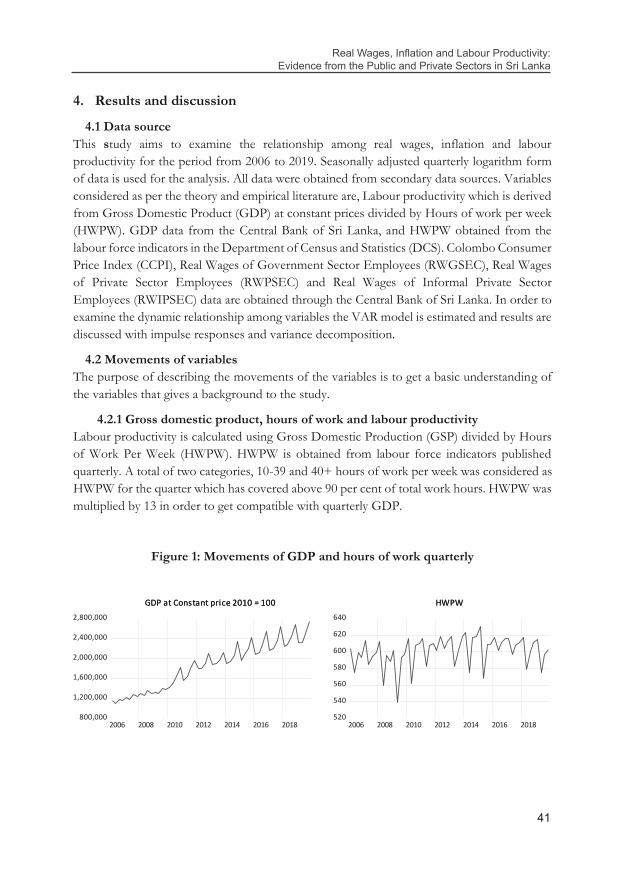
41


41


4.1 Data source This study aims to examine the relationship among real wages, inflation and labour productivity for the period from 2006 to 2019. Seasonally adjusted quarterly logarithm form of data is used for the analysis. All data were obtained from secondary data sources. Variables considered as per the theory and empirical literature are, Labour productivity which is derived from Gross Domestic Product (GDP) at constant prices divided by Hours of work per week (HWPW). GDP data from the Central Bank of Sri Lanka, and HWPW obtained from the labour force indicators in the Department of Census and Statistics (DCS). Colombo Consumer Price Index (CCPI), Real Wages of Government Sector Employees (RWGSEC), Real Wages of Private Sector Employees (RWPSEC) and Real Wages of Informal Private Sector Employees (RWIPSEC) data are obtained through the Central Bank of Sri Lanka. In order to examine the dynamic relationship among variables the VAR model is estimated and results are discussed with impulse responses and variance decomposition.

4.2 Movements of variables The purpose of describing the movements of the variables is to get a basic understanding of the variables that gives a background to the study.

4.2.1 Gross domestic product, hours of work and labour productivity Labour productivity is calculated using Gross Domestic Production (GSP) divided by Hours of Work Per Week (HWPW). HWPW is obtained from labour force indicators published quarterly. A total of two categories, 10-39 and 40+ hours of work per week was considered as HWPW for the quarter which has covered above 90 per cent of total work hours. HWPW was multiplied by 13 in order to get compatible with quarterly GDP.

Figure 1: Movements of GDP and hours of work quarterly

800,000

1,200,000

1,600,000

2,000,000

2,400,000

2,800,000

2006 2008 2010 2012 2014 2016 2018

GDP at Constant price 2010 = 100GDP at Constant price 2010 = 100

520

540

560

580

600

620

640

2006 2008 2010 2012 2014 2016 2018

HWPWHWPW


42

42

As depicted in figure 1, GDP at constant prices has increased over the period. If we consider the GDP growth rate, the growth rate is averaged to 5% during the period from 2006 to 2019, while growth has been limited to below 4-3 per cent recently. Hours of work per quarter averaged to 600 or per week 46 hours. In order to increase labour productivity, numerator, GDP can be increased with a same level of hours of work or with a same level of GDP, the denominator can be decreased. Practically, the number of hours of work is stable or can slightly be changed. Therefore, GDP must be increased to enhance labour productivity. Therefore, slowing down the economic growth means that productivity has also declined compared to the previous year. As per the above graph, it shows a decline in slightly hours of work after 2015. Labour productivity (GDP/HWPW) and the movements in CCPI are given below.

Figure 2: Labour productivity and inflation

Figure 2 depicts the labour productivity (GDP/HWPW) and Consumer Price Index for the period from 2006 to 2019. During the period, both inflation and labour productivity marginally increased. Increase in LPDCT is driven mainly by increase in GDP. The gap between labour productivity and Consumer price index has narrowed mainly due to inflation that has been managed at below 5 per cent.

4.2.2 Labour productivity and real wages

Real Wage Index of Government Sector (RWGSEC), Real Wage Index of Private Sector (RWPSEC) and Real Wage Index of Informal Private Sector employees are considered covering all sectors in the economy. For RWGSEC and RWIPSEC the base year is 2012 = 100, while the base year for RWPSEC is 1978 = 100. RWPSEC covered only the workers in wages board and trades. Movements of indices are discussed with labour productivity. RWGSEC and RWPSEC and REIPSEC are discussed separately.

7.4

7.6

7.8

8.0

8.2

8.4

2006 2008 2010 2012 2014 2016 2018

LPDCTLPDCT

3.8

4.0

4.2

4.4

4.6

4.8

5.0

2006 2008 2010 2012 2014 2016 2018

LCCPILCCPI

43


43

Figure 3: Movements of labour productivity, real wages of government and private sector employees

4.2

4.3

4.4

4.5

4.6

4.7

4.8

4.9

5.0

5.1

06 07 08 09 10 11 12 13 14 15 16 17 18 19

LRWGSEC LRWPSEC LRWIPSEC As per figure 3, productivity has gradually increased over the period while real wage indices of GSEC and PSEC have fluctuated during the period. REIPSEC has always moved above or in line with CCPI movements. The gap between two the Wage indices (RWGSEC and RWPSEC) narrows by 2012, and then it shows the equal movements in wage indexes up to 2014 in several years. After 2014 Q3, a stable parallel gap widens towards 2019 with respect to RWGSEC, RWPSEC and RWIPSEC. It is clear that after 2015 RWGSEC are higher compared to RWPSEC with increase of salary allowances in Government budget proposal that continued to 2020.

Real wages in PSEC declined compared to real wages of other two sectors. Private sector, being 43.4% remains the main employment generating sector in Sri Lanka and public sector contributed 20% to the total employment as per the DCS. Real wages of PSEC is lower compared to the GSEC and IPSEC. Further, after 2015 real wages of GSEC and PSEC assume a declining trend that shows wage pressure in the market. Wages are determined by the Wages Board for RWPSEC and the circulars issued by the Department of public administration for RWGSEC employees, showing some rigidities and sticky adjustment with the market compared to the both CCPI and REIPSEC. A continuous increase of the Real wages of informal private sector employees can be noticed since wages of IPSEC are determined by the market forces. As per the theory and empirical evidence, there is a positive significant relationship between labour productivity and real wages. Therefore, declining real wages would impact labour productivity negatively. Further, a massive salary increases for GSEC employees in 2015 has also impacted a decline in their real wages from 2015 to 2019. Therefore, the continuation of a sustainable wage increasing proposal is important to avoid real wage erosion and minimize differences with real wages of other sectors and to enhance productivity to a significant level.


44

44

4.3 Empirical tests Since time series data has special properties with time varying/ time ordered, it is required to check whether the series’ mean, variance and covariance are the same over the period. In order to check stationarity, ADF (Augmented Dickey-Fuller), PP (Phillips-Perron) and KPSS (Kwiatkowski–Phillips–Schmidt–Shin (KPSS) tests are performed to check the stationarity of variables. Accordingly, all variables are integrated at their first difference and therefore, can be identified as level (1) variables. Since variables are not integrated at I(0), it is required to check whether cointegration exists among variables.

4.4 Cointegration test If all variables are not stationary in level, it should be tested whether the variables are in equilibrium in the long run that we call the existing cointegration. Since all variables are not I (0) and integrated at their first difference, it is required to check whether a long run relationship exists among variables. To check cointegration, the Johansen methodology is used. Cointegration is detected in the Johansen methodology using two tests called the Trace test and the Eigen Value test. In this study, as per both test statistics, it has indicated no cointegration, and therefore the VAR model using first difference of the variables is decided as an appropriate technique to estimate the relationship among variables.

After estimating the VAR model, other tests to check appropriateness and robustness of the model, stability and residual test are performed. Results of the pre-test, stability and residual test are in Annexure.

4.5 Estimating Ordinary Least Squared (OLS) regression OLS is a type of linear least squares method for estimating the unknown parameters in a linear regression model. OLS selects the parameters of a linear function of a set of explanatory variables by the principle of least squares, minimizing the sum of the squares of the differences between the observed dependent variable in the given dataset and those predicted by the linear function. The OLS estimator is consistent when the regressors are exogenous, and optimal in the class of linear unbiased estimators when the errors are homoscedastic and serially uncorrelated. Under these conditions, the method of OLS provides minimum-variance mean-unbiased estimation, Best Linear Unbiased Estimator (BLUE) when the errors have finite variances. Under the additional assumption, the errors are normally distributed; OLS is the maximum likelihood estimator. Therefore, before estimating the VAR, Ordinary Least Square (OLS) estimation for the variables is performed to establish the linear static relationship among variables. The dependent variable is Labour productivity (LPDCT) and the independent variables are Colombo Consumer Price index (CCPI), real wages of government sector (RWGSEC), real wages of private sector (RWPSE) and real wages of informal private sector employee (RWIPSEC).

45


45

Results of the OLS regression are given below.

DLPDCT =β0 +β1 DLCCPI +β2DLRWGSEC+β3DLRWPSEC+β4DLRWIPSEC +e

= 0.008909 ̶̶ 0.029516 DLCCPI ̶̶ 0.128175DLRWGSEC + 0.237700DLRWPSEC + 0.690758DLRWIPSEC

t stat

(0.749401) (-0.057955) (-0.617124) (1.991358) (1.471382)

As per the OLS results, there is a positive significant relationship between labour productivity growth and real wages in private sector employees. As per the theory and empirical evidence, a positive relationship between labour productivity and real wages is established. In this study, the positive relationship between DLPDCT and DLRWPSEC and DLRWIPSEC is examined. The inverse relationship between labour productivity and inflation is in line with the expected results in empirical evidence but not significant. Real wages in government sector employees negatively impact labour productivity. If the results are quantified, a 1 per cent increase in growth of real wages in private sector employees is impacted to increase labour productivity by 0.23 per cent, on average subject to the assumption under ceteris paribus.

Findings support establishing a positive relationship between labour productivity and real wages which is in line with the theory and empirical literature. Therefore, increasing real wages of PSEC and IPSEC employees leads to an increase in productivity higher than increasing real wages of GSEC employees. Inflation negatively but not significantly impacts to enhance labour productivity for the research period covered from 2006 to 2019.

4.6 Estimating the VAR model In order to estimate a VAR model, firstly, the difference of all variables must be considered due to the absence of cointegration and because all variables are integrated at first difference. Then, appropriate lag length must be determined to indicate the dynamic adjustment of variables in the model. Lower lag length results in autocorrelation of the error term to a significant level and insignificant estimators. Higher lag would lead to reduce the degrees of freedom and thereby to estimate insignificant coefficients. Therefore, appropriate lag length is selected based on the LR Sequential modified LR test statistics, FPE Final Prediction Error, AIC Akaike Information Criterion, SC: Schwarz Information Criterion, HQ: Hannan -Quinn Information Criterion to decide appropriate lag length for the model. Lag order 7th is selected based on AIC. The VAR model using the first difference of the variables is estimated under fulfilment of the conditions in lag exclusion test, stability test and residual test performed and are in annex 1. Estimated results of the VAR model are discussed in below sections since


46

45

results of the pre-tests, stability and residual test (Gujarati) for the estimated model fulfil the requirements4 under the Gauss Markov theorem to have estimators with BLUE5 properties.

4.7 Impulse Response Functions (IRF) and Forecast Error Variance Decompositions (FEVD)

In the above estimated VAR model, results are discussed using impulse response functions and forecast error variance decompositions. An impulse response function shows the reaction of any dynamic system in response to external change/ shock. Therefore, the impulse response describes the reaction of the system as a function of time. In the study impulse responses indicate how each variable in the model would behave in response to a shock for variables of LPDCT, LCCPI, LRWGSEC, LRWPSEC and LRWIPSEC.

Figure 4: Impulse response functions: Impulses from DLPDCT, DLCCPI, DLRWGSEC, DLRWPSEC, DLRWIPSEC

4 The error term has a population mean of zero, All independent variables are uncorrelated with the error term, no endogeneity, Observations of the error term are independently distributed and uncorrelated with each other, no autocorrelation/ serial correlation, The error term has a constant variance, no heteroscedasticity Independent variable is not a perfect linear function of other explanatory variables, no multicollinearity 5 Best Linear Unbiased Estimator

-‐.04

-‐.02

.00

.02

2 4 6 8 10 12 14 16 18 20

Response of DLPDCT to DLPDCTResponse of DLPDCT to DLPDCT

-‐.04

-‐.02

.00

.02

2 4 6 8 10 12 14 16 18 20

Response of DLPDCT to DLCCPIResponse of DLPDCT to DLCCPI

-‐.04

-‐.02

.00

.02

2 4 6 8 10 12 14 16 18 20

Response of DLPDCT to DLRWGSECResponse of DLPDCT to DLRWGSEC

-‐.04

-‐.02

.00

.02

2 4 6 8 10 12 14 16 18 20

Response of DLPDCT to DLRWPSECResponse of DLPDCT to DLRWPSEC

-‐.04

-‐.02

.00

.02

2 4 6 8 10 12 14 16 18 20

Response of DLPDCT to DLRWIPSECResponse of DLPDCT to DLRWIPSEC

-‐.010

-‐.005

.000

.005

.010

2 4 6 8 10 12 14 16 18 20

Response of DLCCPI to DLPDCTResponse of DLCCPI to DLPDCT

-‐.010

-‐.005

.000

.005

.010

2 4 6 8 10 12 14 16 18 20

Response of DLCCPI to DLCCPIResponse of DLCCPI to DLCCPI

-‐.010

-‐.005

.000

.005

.010

2 4 6 8 10 12 14 16 18 20

Response of DLCCPI to DLRWGSECResponse of DLCCPI to DLRWGSEC

-‐.010

-‐.005

.000

.005

.010

2 4 6 8 10 12 14 16 18 20

Response of DLCCPI to DLRWPSECResponse of DLCCPI to DLRWPSEC

-‐.010

-‐.005

.000

.005

.010

2 4 6 8 10 12 14 16 18 20

Response of DLCCPI to DLRWIPSECResponse of DLCCPI to DLRWIPSEC

-‐.02

.00

.02

2 4 6 8 10 12 14 16 18 20

Response of DLRWGSEC to DLPDCTResponse of DLRWGSEC to DLPDCT

-‐.02

.00

.02

2 4 6 8 10 12 14 16 18 20

Response of DLRWGSEC to DLCCPIResponse of DLRWGSEC to DLCCPI

-‐.02

.00

.02

2 4 6 8 10 12 14 16 18 20

Response of DLRWGSEC to DLRWGSECResponse of DLRWGSEC to DLRWGSEC

-‐.02

.00

.02

2 4 6 8 10 12 14 16 18 20

Response of DLRWGSEC to DLRWPSECResponse of DLRWGSEC to DLRWPSEC

-‐.02

.00

.02

2 4 6 8 10 12 14 16 18 20

Response of DLRWGSEC to DLRWIPSECResponse of DLRWGSEC to DLRWIPSEC

-‐.02

.00

.02

2 4 6 8 10 12 14 16 18 20

Response of DLRWPSEC to DLPDCTResponse of DLRWPSEC to DLPDCT

-‐.02

.00

.02

2 4 6 8 10 12 14 16 18 20

Response of DLRWPSEC to DLCCPIResponse of DLRWPSEC to DLCCPI

-‐.02

.00

.02

2 4 6 8 10 12 14 16 18 20

Response of DLRWPSEC to DLRWGSECResponse of DLRWPSEC to DLRWGSEC

-‐.02

.00

.02

2 4 6 8 10 12 14 16 18 20

Response of DLRWPSEC to DLRWPSECResponse of DLRWPSEC to DLRWPSEC

-‐.02

.00

.02

2 4 6 8 10 12 14 16 18 20

Response of DLRWPSEC to DLRWIPSECResponse of DLRWPSEC to DLRWIPSEC

-‐.010

-‐.005

.000

.005

.010

2 4 6 8 10 12 14 16 18 20

Response of DLRWIPSEC to DLPDCTResponse of DLRWIPSEC to DLPDCT

-‐.010

-‐.005

.000

.005

.010

2 4 6 8 10 12 14 16 18 20

Response of DLRWIPSEC to DLCCPIResponse of DLRWIPSEC to DLCCPI

-‐.010

-‐.005

.000

.005

.010

2 4 6 8 10 12 14 16 18 20

Response of DLRWIPSEC to DLRWGSECResponse of DLRWIPSEC to DLRWGSEC

-‐.010

-‐.005

.000

.005

.010

2 4 6 8 10 12 14 16 18 20

Response of DLRWIPSEC to DLRWPSECResponse of DLRWIPSEC to DLRWPSEC

-‐.010

-‐.005

.000

.005

.010

2 4 6 8 10 12 14 16 18 20

Response of DLRWIPSEC to DLRWIPSECResponse of DLRWIPSEC to DLRWIPSEC

Response to Cholesky One S.D. (d.f. adjusted) Innovations ± 2 S.E.Response to Cholesky One S.D. (d.f. adjusted) Innovations ± 2 S.E.

45

results of the pre-tests, stability and residual test (Gujarati) for the estimated model fulfil the requirements4 under the Gauss Markov theorem to have estimators with BLUE5 properties.

4.7 Impulse Response Functions (IRF) and Forecast Error Variance Decompositions (FEVD)

In the above estimated VAR model, results are discussed using impulse response functions and forecast error variance decompositions. An impulse response function shows the reaction of any dynamic system in response to external change/ shock. Therefore, the impulse response describes the reaction of the system as a function of time. In the study impulse responses indicate how each variable in the model would behave in response to a shock for variables of LPDCT, LCCPI, LRWGSEC, LRWPSEC and LRWIPSEC.

Figure 4: Impulse response functions: Impulses from DLPDCT, DLCCPI, DLRWGSEC, DLRWPSEC, DLRWIPSEC

4 The error term has a population mean of zero, All independent variables are uncorrelated with the error term, no endogeneity, Observations of the error term are independently distributed and uncorrelated with each other, no autocorrelation/ serial correlation, The error term has a constant variance, no heteroscedasticity Independent variable is not a perfect linear function of other explanatory variables, no multicollinearity 5 Best Linear Unbiased Estimator

-‐.04

-‐.02

.00

.02

2 4 6 8 10 12 14 16 18 20

Response of DLPDCT to DLPDCTResponse of DLPDCT to DLPDCT

-‐.04

-‐.02

.00

.02

2 4 6 8 10 12 14 16 18 20

Response of DLPDCT to DLCCPIResponse of DLPDCT to DLCCPI

-‐.04

-‐.02

.00

.02

2 4 6 8 10 12 14 16 18 20

Response of DLPDCT to DLRWGSECResponse of DLPDCT to DLRWGSEC

-‐.04

-‐.02

.00

.02

2 4 6 8 10 12 14 16 18 20

Response of DLPDCT to DLRWPSECResponse of DLPDCT to DLRWPSEC

-‐.04

-‐.02

.00

.02

2 4 6 8 10 12 14 16 18 20

Response of DLPDCT to DLRWIPSECResponse of DLPDCT to DLRWIPSEC

-‐.010

-‐.005

.000

.005

.010

2 4 6 8 10 12 14 16 18 20

Response of DLCCPI to DLPDCTResponse of DLCCPI to DLPDCT

-‐.010

-‐.005

.000

.005

.010

2 4 6 8 10 12 14 16 18 20

Response of DLCCPI to DLCCPIResponse of DLCCPI to DLCCPI

-‐.010

-‐.005

.000

.005

.010

2 4 6 8 10 12 14 16 18 20

Response of DLCCPI to DLRWGSECResponse of DLCCPI to DLRWGSEC

-‐.010

-‐.005

.000

.005

.010

2 4 6 8 10 12 14 16 18 20

Response of DLCCPI to DLRWPSECResponse of DLCCPI to DLRWPSEC

-‐.010

-‐.005

.000

.005

.010

2 4 6 8 10 12 14 16 18 20

Response of DLCCPI to DLRWIPSECResponse of DLCCPI to DLRWIPSEC

-‐.02

.00

.02

2 4 6 8 10 12 14 16 18 20

Response of DLRWGSEC to DLPDCTResponse of DLRWGSEC to DLPDCT

-‐.02

.00

.02

2 4 6 8 10 12 14 16 18 20

Response of DLRWGSEC to DLCCPIResponse of DLRWGSEC to DLCCPI

-‐.02

.00

.02

2 4 6 8 10 12 14 16 18 20

Response of DLRWGSEC to DLRWGSECResponse of DLRWGSEC to DLRWGSEC

-‐.02

.00

.02

2 4 6 8 10 12 14 16 18 20

Response of DLRWGSEC to DLRWPSECResponse of DLRWGSEC to DLRWPSEC

-‐.02

.00

.02

2 4 6 8 10 12 14 16 18 20

Response of DLRWGSEC to DLRWIPSECResponse of DLRWGSEC to DLRWIPSEC

-‐.02

.00

.02

2 4 6 8 10 12 14 16 18 20

Response of DLRWPSEC to DLPDCTResponse of DLRWPSEC to DLPDCT

-‐.02

.00

.02

2 4 6 8 10 12 14 16 18 20

Response of DLRWPSEC to DLCCPIResponse of DLRWPSEC to DLCCPI

-‐.02

.00

.02

2 4 6 8 10 12 14 16 18 20

Response of DLRWPSEC to DLRWGSECResponse of DLRWPSEC to DLRWGSEC

-‐.02

.00

.02

2 4 6 8 10 12 14 16 18 20

Response of DLRWPSEC to DLRWPSECResponse of DLRWPSEC to DLRWPSEC

-‐.02

.00

.02

2 4 6 8 10 12 14 16 18 20

Response of DLRWPSEC to DLRWIPSECResponse of DLRWPSEC to DLRWIPSEC

-‐.010

-‐.005

.000

.005

.010

2 4 6 8 10 12 14 16 18 20

Response of DLRWIPSEC to DLPDCTResponse of DLRWIPSEC to DLPDCT

-‐.010

-‐.005

.000

.005

.010

2 4 6 8 10 12 14 16 18 20

Response of DLRWIPSEC to DLCCPIResponse of DLRWIPSEC to DLCCPI

-‐.010

-‐.005

.000

.005

.010

2 4 6 8 10 12 14 16 18 20

Response of DLRWIPSEC to DLRWGSECResponse of DLRWIPSEC to DLRWGSEC

-‐.010

-‐.005

.000

.005

.010

2 4 6 8 10 12 14 16 18 20

Response of DLRWIPSEC to DLRWPSECResponse of DLRWIPSEC to DLRWPSEC

-‐.010

-‐.005

.000

.005

.010

2 4 6 8 10 12 14 16 18 20

Response of DLRWIPSEC to DLRWIPSECResponse of DLRWIPSEC to DLRWIPSEC

Response to Cholesky One S.D. (d.f. adjusted) Innovations ± 2 S.E.Response to Cholesky One S.D. (d.f. adjusted) Innovations ± 2 S.E.

47


Impulse response functions for the variables are within the dotted lines, implying the significance of the movements towards the time periods. One shock to DLPDCT has initially a noticeable impact on DLPDCT itself in the current period and its minimum level is recorded in the 3rd quarter. In the medium run, growth of the LPDCT fluctuates, which stabilizes in the long-run with a lower level than the original. Therefore, it can be concluded that any shock to growth of the LPDCT leads to a decline in the growth of LPDCT drastically in the short run and in the long run as well. A sudden shock in DLPDCT has a noticeable impact and increases inflation, implying a negative effect between variables. As per the theory and empirical studies, inflation negatively impacts on economic activity and labour productivity as well. Many of the empirical studies(Clark; Bårdsen, Hurn and McHugh; Buck and Fitzroy; Christopoulos and Tsionas; De Gregorio; Narayan and Smyth; Smyth) conclude that there is a negative relationship between inflation and productivity. (Hondroyiannis and Papapetrou “Seasonality-Cointegration and the Inflation, Productivity and Wage Growth Relationship in Greece”) examine the relationship during the period 1975-1992 and found that in the short-run, dynamic results are indicative of a negative effect of inflation on productivity. The finding of the dynamic relationship between inflation and labour productivity in this study using VAR, is in line with empirical studies. Therefore, avoiding negative shock to productivity (GDP/HWPW) leads to managing inflation in the short run.

A shock from DLPDCT has a noticeable impact to decline real wages in all sectors. As per the theory and empirical evidence, a positive relationship between labour productivity and real wages has been established. The positive relationship between real wages and labour productivity is further confirmed by (Kumar, Webber and Perry) in their study on Real wages, inflation and labour productivity in Australia for 1965-2007; it is quantified that a 1% increase in real wages of manufacturing sector is expected to increase productivity between 0.5% and 0.8%, implying a positive significant relationship between wages and productivity while the effect of inflation on manufacturing sector productivity is not significant. In line with the same, (Narayan and Smyth) also confirm that a 1% increase in real wages generates a 0.6% increase in productivity while effects of inflation on productivity are insignificant. (Eryılmaz and Bakır) examine real wages, inflation and labour productivity, an evaluation within the Turkish context during the period of 1988-2012 and reveal that there is a long-term relationship among variables from productivity and inflation towards the real wages. Therefore, the findings of the relationship between real wages and labour productivity are in line with the theory and the empirical evid-ence. In this study findings refer to short run analysis followed by VAR.

Impulses from inflation have a noticeable impact on the decline and volatility of DLPDCT, increase real wages in Government and Informal private sector employees and decrease real wages in private sector employees. Impulses from real wages in Government sector employees are led to decrease and make volatile DLPDCT and inflation while leading real wages in other sectors to increase in the short run. A sudden shock in LRWPSEC has a noticeable impact in terms of increasing inflation and real wages in other sectors in the short run. Impulses from real wages in informal private sector impact to decline labour productivity growth and inflation in the medium run and fluctuate other sector real wages.


48 47

In conclusion, the impulses of LPDCT, LCCPI, LRWGSEC, LRWPSE and LRWIPSEC on other variables have a noticeable impact in the short run while shocks die out in the long run. A positive relationship between labour productivity and real wages, and a negative relationship between labour productivity and inflation can be noticed as per the impulse response functions. Further, higher inflation leads to increase in real wages in the Government and informal private sectors while private sector wages marginally increase. Therefore, policy measures must be identified to ensure minimum shock on LPDCT to achieve long-term economic growth. In this, keeping a well-managed lower level inflation will have a minimum impact on other variables since lower inflation causes a higher growth rate, lower growth of real wages in GSEC, IPSEC and minimum shocks to Real wages of PSEC employees.

4.8 Forecast Error Variance Decomposition (FEVD) on main variable This helps to determine the proportion of variation of the dependent variable explained by each of the independent variables. Variance decomposition enables to determine how much of the variability of the independent variable is lagged by its own variance. In addition, it shows you which of the independent variables is ‘stronger’ in explaining the variability in the dependent variables over the period. This evolves over time, so the shocks on time series variables may not be very important in the short-run but very important in the long run. On the other hand, the error variance decomposition shows how the importance of each shock explains the fluctuations in the variables in the model for the above variables. Accordingly, FEVDs are described below.

Table 1: Variance Decomposition of LPDCT

Period S.E. LPDCT LCCPI LRWGSEC LRWPSEC LRWIPSEC

1 0.029000 100.0000 0.000000 0.000000 0.000000 0.000000 2 0.035197 88.43588 5.233029 4.036736 1.937992 0.356360 3 0.039014 72.31407 17.52198 8.059185 1.625107 0.479661 4 0.042500 61.89649 23.67407 8.929126 4.882714 0.617602 5 0.047561 58.53307 19.11381 14.71565 6.380837 1.256630 6 0.053517 47.30266 18.49453 19.90920 5.065957 9.227654 7 0.055559 44.04469 19.09424 20.14761 4.767954 11.94550 8 0.058842 39.64846 19.88812 23.17052 6.412053 10.88085 9 0.060799 37.13731 21.41000 24.44272 6.150542 10.85944 10 0.063670 38.32583 19.56755 26.04983 5.983782 10.07301

49


48

FEVD indicates the amount of information each variable contributes to the other variables in the VAR model. In Table 1, variance decomposition of growth of LPDCT to other time series is given. It shows that, in the current period, DLPDCT is a strongly endogenous variable. Gradually, total variance is explained, in DRWGSEC, DLCCPI, DLRWIPSEC and DLRWPSEC in the long run, shows a strong influence on other variables. Over the period DLRWGSEC and DLCCPI variables reflect a higher percentage of variation of LPDCT in the long run. Only about 6% of the variance in DLPDCT is explained by DLRWPSEC.

4.9 Forecast error variance decomposition on other variables LCCPI has a strong influence on dependent variables, and therefore, can be identified as a strongly exogenous variable, since its variance reflects around 1-42 per cent in LPDCT and other variables. Variations in LCCPI are explained by LPDCT gradually towards the long run. Real wages of all three sectors have less variance of around 7% in LCCPI variance decomposition compared to LPDCT. Forecast error variance of RWGSEC, RWPSEC and RWIPSEC are in the annexures. As per FEVD of DLRWGSEC, 30-40 per cent variance in DLRWGSEC is explained by inflation and by DLPDCT. Error variance of DLPSEC is explained above 20 per cent by DLPDCT, and the least amount reflects in DLCCPI. About 60 - 40 per cent variance is explained by DLCCPI in FEVD of DLWRIPSEC. Accordingly, real wage increase in the private sector will enhance productivity with a minimum impact on inflation. Real wage increase in the Government sector will be reflected in inflation and in labour productivity.

Table 2: Variance decomposition of LCCPI

Period S.E. LPDCT LCCPI LRWGSEC LRWPSEC LRWIPSEC

1 0.010326 0.177803 99.82220 0.000000 0.000000 0.000000 2 0.014073 18.04624 73.97567 2.417170 4.700750 0.860173 3 0.014917 16.29932 75.34729 3.382805 4.204084 0.766502 4 0.015233 15.67582 74.58858 3.336973 4.190810 2.207825 5 0.015710 17.35756 70.28773 4.691908 5.532001 2.130801 6 0.015889 17.36766 68.95696 5.483103 5.574071 2.618201 7 0.016866 21.39691 62.43460 4.867201 6.603524 4.697768 8 0.017402 22.37063 58.68848 6.326622 6.726889 5.887373 9 0.018332 20.92091 59.53429 5.853680 6.121767 7.569354 10 0.018623 20.30051 58.06721 6.404412 7.719534 7.508337

4.10 Granger causality Direction of causality was examined using the Block exogeneity test. It explains whether lag values of X variable are helpful in explaining Y variable. The null hypothesis of the non - existence of a Granger causality between variables is rejected with p value lower than 0.05 level. Accordingly, the following causality relationships can be identified.


50

50

Figure 5: Causal relationship among variables

DLPDCT DLCCPI

DLRWPSECDLRWGSEC

As per Figure 5, one directional causality is identified as productivity growth Granger causes inflation at a 5 per cent significance level. Accordingly, lag values of productivity growth help to better predict inflation. Findings support the view that the productivity Ganger causes inflation in standard economic theory. (Kim, Lim and Park) also finds unidirectional Granger causality from productivity growth to inflation in Korea. (Jarrett and Selody) finds two-way causality from inflation to productivity for aggregate quarterly data in Canada. (Strauss and Wohar) examine the long run relationship between inflation, real wages and productivity in the US and findings were, in the long run, inflation Granger causes productivity and there is a bidirectional Granger causality between real wages and productivity. Further, in this study, there is a one directional causality from inflation towards real wage growth in the private sector, from DLRWGSEC towards DLRWPSEC. Therefore, past values of inflation and DLRWGSEC help to better predict current DLRWPSEC than past values of DLRWPSEC alone.

5. Conclusion and recommendations

The aim of this study is to examine and analyse the relationship among real wages, inflation and labour productivity in Sri Lanka during the period from 2006 to 2019 using secondary data sources. Other objectives are to identify key factors affecting labour productivity with inflation and sector wise real wages (GSEC, PSEC & IPSEC) and to identify the sector wise contribution to the labour productivity separately. In order to examine the static and dynamic relationship among variables, OLS regression and the VAR model were employed. Number of studies on real wages, inflation and labour productivity has been conducted covering developed and developing countries. Findings of the relationships between variables ends with mixed results. Majority of the studies have concluded that real wages positively impact labour

51


51

productivity while inflation has a negative impact in the short run or long run basis. This study was the initial study on real wages, inflation and labour productivity in Sri Lanka. Accordingly, there is a short run relationship among real wages, inflation and labour productivity. A negative relationship is identified between labour productivity and inflation while a positive relationship is identified between labour productivity and real wages in all three sectors in Sri Lanka during the period.

As per the IRF, a sudden shock in LPDCT has a noticeable impact to decline productivity itself, to increase inflation, and to decline real wages of all sectors by stabilising lower real wages in the long run. Results of the OLS regression are also in line with the findings of the VAR model which are reflected in the dynamic analysis. Accordingly, a negative relationship between labour productivity and inflation, and a positive relationship between real wages and inflation are established. Each of the IRFs on other variables are helpful to identify possible policy measures. Impulses on LPDCT lead to increases in inflation while causing real wages to decline. Impulses on LCCPI lead to decline of LPDCT, increase of real wages in GSEC, IPSEC while RWPSEC employees are not impacted much. Impulses of real wages among sectors are also considered. Impulses on real wages of GSEC and IPSEC employees are positively related with each other reactions. Impulses on RWPSEC are negatively related with the other two. In order to enhance labour productivity, increasing real wages of RWPSEC employees can be considered since there is a positive significant relationship to enhance productivity as quantify in OLS results and real wages of RWPSEC and inflation indicates less volatilities in LPDCT and LCCPI compared to real wages of the other two sectors. This would help to have a minimum impact on inflation while productivity is enhanced. Therefore, increasing real wages of private sector employees can be recommended as one of the policy measures to enhance labour productivity.

As well-established empirical analyses conclude, an increase in real wages leads to an increase in productivity. There is a positive statistically significant relationship between real wages and labour productivity (Narayan and Smyth; Kumar, Webber and Perry; Katovich and Maia). Therefore, the findings are in line with theory and empirical literature. In this analysis, Real wages of GSEC, PSEC and IPSEC were considered to identify the factors affecting labour productivity sector-wise. Accordingly, RWGSEC, RWPSEC and RWIPSEC employees’ contributions are positive in terms of labour productivity. Further, it can be concluded that the impact to the labour productivity by PSEC and IPSEC employees is higher compared to the GSEC employees. As per the OLS results, there is a negative insignificant relationship between labour productivity and real wages of GSEC employees. Therefore, real wages of GSEC employee’s contribution to labour productivity is not significant. In the VAR analysis too, a positive significant dynamic relationship was identified between labour productivity and real wages of PSEC and IPSEC employees compared to RWGSEC employees. Therefore, in order to enhance labour productivity in GSEC employees to a significant level, identifying, introducing and implementing additional assignable work to the GSEC employees should be


52

52

considered. Otherwise wage increases of GSEC employees will result in increased inflation and have an adverse impact on productivity too. GSEC employees being 20 per cent to the total employment in Sri Lanka should also have a positive significant impact on labour productivity. In this regard, measures in order to further improve labour productivity in GSEC employees are suggested as identifying and assigning more work allocation as per the Government requirement continuously, introducing to achieve targets for work attended compared with number of works received for the possible sectors. This will bring GSEC employees’ contribution to labour productivity towards a positive significant level as PSEC employees.

Relationship between inflation and labour productivity is identified as negative in the short run dynamic in Sri Lanka. Therefore, any negative shock to productivity will increase inflation immediately up to medium run and after that gradually fluctuate towards a higher level than the original while shocks are dying out throughout the period. Based on the negative relationship between labour productivity and inflation, it can be recommended that keeping a lower level of inflation will manage negative shocks to productivity in the short run. Higher inflation adversely impacts productivity in the short run in three ways: worker purchasing power, mix of factor inputs and impact to the investments plans as specified in empirical literature. Further, the sudden shock of inflation will have a noticeable impact to further increase real wages of GSEC and IPSEC employees as well. Real wages of private sector employees are minimally impacted by impulses on LCCPI. Therefore, as pointed out above, in order to enhance productivity, increasing real wages of PSEC employees can be considered. Further, Department of Census and Statistics, identified, PSEC being 43 per cent of the total employment in Sri Lanka, is the employment generating sector of the economy. Therefore, the Government also can further facilitate PSEC by supporting large scale investment projects, modernizing infrastructure facilities, contributing expenses related to research and development, innovations, and safeguarding the private sector.

As per the FEVD function, LPDCT is a strongly endogenous variable in the short run while all other variables are weakly exogenous in the short run. A higher portion of variance in DLPDCT is explained by DLRWGSE and DLCCPI. Further in FEVD of LCCPI, above 20 per cent of variance is explained by DLPCT. FEVD of Real wages in the private sector is explained above 20 percent of variance in productivity growth while the Government sector and informal private sector reflect higher variance in LCCPI. Therefore, FEVD of RWGSEC and RWIPSEC contributes to inflation highly compared to the RWPSEC that has much contribution to the variance of LPDCT. This close relationship between labour productivity and RWPSEC employees, inflation and RWGSEC, RWIPSEC is well established through IRF, FEVD and Granger causality. The private sector can be identified as a key factor of labour productivity as per the findings of this study. Therefore, growth stimulating policies, well- managed inflation, facilitating modern infrastructures, innovations, expenses on research and developments can be considered to encourage, in addition to increasing real wages of private

53


53

sector employees to enhance labour productivity. In FEVD of LPDCT, the contribution of real wages in all sectors is far greater than inflation. In the same way, FEVD of LDPCT is reflected mostly in DLRWPSEC while error variance in LCCPI is highly contributed by LPDCT and RWGSEC.

As per the results of the Granger Causality Block Exogeneity test, three one directional causality relationships were identified. Individually, there is one directional relationship from labour productivity towards inflation. A further one directional relationship exists from inflation towards real wages in private sector employees, from real wages in the Government sector towards real wages in the private sector. Other causality relationships were identified from all variables as jointly Granger cause labour productivity growth and inflation. The finding of the Granger causality running among variables and direction of the causality can be used for the better prediction of the variables, DLPDCT, DLCCPI and DLRWPSEC. This study can be further developed considering a new wage rate index for the private sector, incorporating other variables such as capital stock, technological changes and other factors that could enhance labour productivity.


54

54

References

Alexander, Carol O. "The changing relationship between productivity, wages and unemployment in the UK." Oxford bulletin of economics and statistics 55.1 (1993): 87-102. Print.

Angeles-Castro, Gerardo, Jonatan Juárez-Cruz, and Miguel Flores-Ortega. "The effect of average wages on the economy: the case of the United States." International journal of business and social science 5.11 (2014). Print.

Annual Report 2018: Central Bank of Sri Lanka, 2018. Print.

Annual Report 2019: Central Bank of Sri Lanka, 2019. Print.

Asian Development Bank, International Labour Organization, and Regional Office for Labour the Pacific. "Sri Lanka: fostering workforce skills through education: employment diagnostic study." (2017). Print.

Bårdsen, Gunnar, Stan Hurn, and Zoë McHugh. "Modelling wages and prices in Australia." Economic record 83.261 (2007): 143-58. Print.

Brida, Juan Gabriel, Wiston Adrián Risso, and Edgar J Sanchez Carrera. "Real wages as determinant of labour productivity in the Mexican tourism sector." European journal of tourism research 3.1 (2010): 67. Print.

Bruno, Michael, and William Easterly. "Inflation crises and long-run growth, data set." 1998. Print.

Buck, Andrew J, and Felix Fitzroy. "Inflation and productivity growth in the Federal Republic of Germany." Journal of post Keynesian economics 10.3 (1988): 428-44. Print.

Cameron, Norman, Derek Hum, and Wayne Simpson. "Stylized facts and stylized illusions: inflation and productivity revisited." Canadian journal of economics (1996): 152-62. Print.

Chowdhury, Anis, and Girijasankar Mallik. "A land locked into low inflation–how far is the promised land?" Economic analysis and policy 28.2 (1998): 233-44. Print.

Christopoulos, Dimitris K, and Efthymios G Tsionas. "Productivity growth and inflation in europe: evidence from panel cointegration tests." Empirical economics 30.1 (2005): 137-50. Print.

Clark, Peter K. "Inflation and the productivity decline." The American economic review 72.2 (1982): 149-54. Print.

55


55

De Gregorio, José. "Economic growth in Latin America." Journal of development economics 39.1 (1992): 59-84. Print.

Dritsaki, Chaido. "Real wages, inflation, and labor productivity: evidences from Bulgaria and Romania." Journal of economic & financial studies 4.05 (2016): 24-36. Print.

Engle, Robert F, and Clive WJ Granger. "Co-Integration and Error Correction: Representation, estimation, and testing." Econometrica: journal of the econometric society (1987): 251-76. Print.

Erenburg, Sharon J. "Productivity, private and public capital, and real wage in the US." Applied economics letters 5.8 (1998): 491-95. Print.

Eryılmaz, Filiz, and H Bakır. "Real wages, inflation and labor productivity: an evaluation within Turkish context." Hitit University journal of social sciences institute 11.3 (2018): 1946-59. Print.

Feldstein, Martin. "Did wages reflect growth in productivity?" Journal of policy modeling 30.4 (2008): 591-94. Print.

Freeman, Donald G, and David B Yerger. "Does inflation lower productivity? time series evidence on the impact of inflation on labor productivity in 12 OECD nations." Atlantic economic journal 28.3 (2000): 315-32. Print.

Inflation and multifactor productivity growth: A response to smyth. Applied economics letters 5.5 (1998): 271-74. Print.

Gordon, Robert J. "Productivity, wages, and prices inside and outside of manufacturing in the US, Japan, and Europe." European economic review 31.3 (1987): 685-733. Print.

Granger, Clive WJ, Paul Newbold, and J Econom. "Spurious regressions in econometrics." Baltagi, Badi H. A companion of theoretical econometrics (1974): 557-61. Print.

Gujarati, Damodar N. basic econometrics. Tata McGraw-Hill education, 2009. Print.

Hall, Stephen G. "An application of the granger & engle two‐step estimation procedure to United Kingdom aggregate wage data." Oxford bulletin of economics and statistics 48.3 (1986): 229-39. Print.

Hendry, David F. "Modelling UK inflation, 1875–1991." Journal of applied econometrics 16.3 (2001): 255-75. Print.


56

56

Hondroyiannis, George, and Evangelia Papapetrou. "Seasonality-cointegration and the inflation, productivity and wage growth relationship in Greece." The social science journal 34.2 (1997): 235-47. Print.

Temporal causality and the inflation-productivity relationship: evidence from eight low inflation oecd countries. International review of economics & finance 7.1 (1998): 117-35. Print.

Hsu, Pi-Fem. "Inter-industry wage premiums and industry-specific productivity in Taiwan." Applied economics 37.13 (2005): 1523-33. Print.

Islam, Rizwanul, Abel Kinyondo, and Joseph Nganga. "Real wages and labour productivity in Tanzania: How do they link?" Journal of African studies and development 7.3 (2015): 81-98. Print.

Jarrett, J Peter, and Jack G Selody. "The productivity-inflation nexus in Canada, 1963-1979." The review of economics and statistics (1982): 361-67. Print.

Johansen, Søren. "Statistical analysis of cointegration vectors." Journal of economic dynamics and control 12.2-3 (1988): 231-54. Print.

Katovich, Erik S, and Alexandre Gori Maia. "The relation between labor productivity and wages in Brazil: A sectoral analysis." Nova economia 28.1 (2018): 7-38. Print.

Kim, Doh-Khul. "Real wage and nominal shock: evidence from Pacific-Rim countries." International advances in economic research 11.3 (2005): 249-55. Print.

Kim, Sangho, Hyunjoon Lim, and Donghyun Park. "Does productivity growth lower inflation in Korea?" Applied economics 45.16 (2013): 2183-90. Print.

Klein, Nir. real wage, labor productivity, and employment trends in South Africa: A closer look. International Monetary Fund, 2012. Print.

Krugman, Paul R. The age of diminished expectations: US economic policy in the 1990s. MIT press, 1997. Print.

Kumar, Saten, Don J Webber, and Geoff Perry. "Real wages, inflation and labour productivity in Australia." Applied economics 44.23 (2012): 2945-54. Print.

Liew, Venus Khim-Sen. "Which lag length selection criteria should we employ?" Economics bulletin 3.33 (2004): 1-9. Print.

57


57

Maia, Alexandre Gori, and Arthur Sakamoto. "Does wage reflect labor productivity? a comparison between Brazil and the United States." Brazilian journal of political economy 38.4 (2018): 629-49. Print.

Mehra, Yash P. "Wage growth and the inflation process: an empirical note." The American economic review 81.4 (1991): 931-37. Print.

Mora, Toni, Jordi Lòpez-Tamayo, and Jordi Suriñach. "Are wages and productivity converging simultaneously in Euro area countries?" Applied economics 37.17 (2005): 2001-08. Print.

Narayan, Paresh, and Russell Smyth. "The effect of inflation and real wages on productivity: new evidence from a panel of G7 countries." Applied economics 41.10 (2009): 1285-91. Print.

Papapetrou, Evangelia. "The inflation and productivity relationship in Poland." Journal of economics and business 2003.2 (2003): 11-33. Print.

Phillips, Peter CB, and Sam Ouliaris. "Asymptotic properties of residual based tests for cointegration." Econometrica 58.1 (1990): 165-93. Print.

Pruchnik, Kamil, and Jakub Zowczak. Middle-income trap: review of the conceptual framework: ADBI working paper, 2017. Print.

Sbordone, Argia, and Kenneth Kuttner. "Does inflation reduce productivity?" Federal Reserve Bank of Chicago economic perspectives 18.6 (1994): 2-14. Print.

Shapiro, Carl, and Joseph E Stiglitz. "Equilibrium unemployment as a worker discipline device." The American economic review 74.3 (1984): 433-44. Print.

Smyth, David J. "Inflation and total factor productivity in Germany." Weltwirtschaftliches Archiv 131.2 (1995): 403-05. Print.

Strauss, Jack, and Mark E Wohar. "The linkage between prices, wages, and labor productivity: a panel study of manufacturing industries." Southern economic journal (2004): 920-41. Print.

Tang, Chor Foon. "A note on the non-linear wages-productivity nexus for Malaysia." (2010). Print.

Wakeford , Jeremy. "The productivity–wage relationship in South Africa: An empirical investigation." Development Southern Africa 21.1 (2004): 109-32. Print.

Yildirim, Zekeriya. "Relationships among labour productivity, real wages and inflation in Turkey." Economic research-ekonomska istraživanja 28.1 (2015): 85-103. Print.


58

59

61

Determinants of Microfinance Interest Rates: Case of Sri Lanka

Indeewari U. Colombage1 and Tharanga A.D. Wijayakoon2

Abstrac t

This research attempts to identify determinants of microfinance interest rates with a view to control and reduce such rates for the betterment of microfinance clients. Data from 30 microfinance institutions were gathered using a set format to capture required variables. The variables covered the cost of funds, efficiency, competition and company characteristics. Variables such as return on assets, non-performing accommodations, competition and average loan size were considered as endogenous. Therefore, a two stage least square panel regression using random effects was used to analyse the data. The identified determinants of microfinance interest rates were the prior period’s interest rate, cost of funds, efficiency, the size of firm and profitability. However, competition, the nature of microfinance institution and the experience of the firm did not give significant results. Accordingly, it is recommended that appropriate action should be taken to reduce the cost of funds, improve efficiency and transmit the profitability of institutions to the microfinance client. Further, policies should be developed to improve transparency in the pricing imposed by such institutions and to enhance financial literacy of the public to derive benefits of competition. Thereby, the size of firm, experience and regulatory position can be stimulated to minimize interest rates.

Key Words : Competition, Cost of Funds, Efficiency, Microfinance Institutions, Interest Rates

1The author is currently serving as a Senior Assistant Director of the Department of Macroprudential Surveillance at the Central Bank of Sri Lanka. Corresponding email: [email protected] 2 The author is currently serving as a Senior Assistant Director of the Department of Supervision of Non-Bank Financial Institutions at the Central Bank of Sri Lanka. Corresponding email: [email protected]. authors are thankful to the anonymous reviewers for their comments and advice. The views presented in this paper are those of the author and do not necessarily indicate the views of the Central Bank of Sri Lanka. the authors and do not necessarily indicate the views of the Central Bank of Sri Lanka.

Abstract

Key Words: Competition, Cost of Funds, Efficiency, Microfinance Institutions,

Interest Rates


60

62

1. Introduction

Microfinance is defined by the Consultative Group to Assist the Poor (CGAP) as “provision of financial services to low-income people”, CGAP (2017). This could include provision of credit, savings facilities, insurance and pension products, money transfer services, and training and consultation services. Banks have traditionally considered low-income persons as 'unbankable' as they have no conventional collateral to offer and micro-enterprises operated by such persons are rather small and risky. Microfinance Institutions (MFIs) provide access to finance for such individuals. However the role of microfinance extends beyond simply providing access to finance and thereby increasing financial inclusion. MFIs empower their clients by providing various training and development opportunities (Zerai & Rani 2011), to better utilize their finances. Microfinance, through employment generation empowers clients, helps reduce poverty, and helps reduce inequality in wealth distribution (Cotler & Almazan 2013).

In the 1970s, MFIs required substantial subsidies to serve their clients (Morduch et al. 2009). Therefore, as Lingerwood (2001) and Xhristen (1997) note, during this period microfinance projects were entirely donor funded with limitations on funds, time, economic activity and geographical location (as cited by Kipesha & Zhang 2013). In the 1980s and 1990s policy makers argued that MFIs should be profitable/financially sustainable (Morduch et al. 2009). It was argued that access to finance is more important than the price, and any price MFIs charge is justified, if it is below what the local money lenders charge (ibid.). According to this premise, both non-profit and for-profit MFIs were encouraged to raise interest rates. However, such high interest rates have not resulted in increased profits for MFIs (Roberts 2013). High rates of default, higher administration costs and policies of low interest rates were assumed to prevent MFIs from being profitable (Sanderatne 2007). According to Mardoch (2000) and Ottero (1999), MFIs continued to be affected by dependence on donor funds and poor fund management (as cited by Kipesha & Zhang 2013). This resulted in an argument for more efficient and sustainable MFIs (Kipesha & Zhang 2013). According to Christen (2001), Isern & Porteous (2006) and Ryne (1998), a profitable MFI would be able to reach more people while being less dependent on donor funds (as cited by Kipesha & Zhang, 2013). However, in Sri Lanka, both not-for-profit Non-Governmental organizations as well as for-profit MFIs operate parallelly.

Emphasis on financial sustainability has resulted in the number of for-profit MFIs increasing (Roberts, 2013). With the emphasis on profitability, the social objective of poverty alleviation of MFIs has moved towards the economic objective of providing sustainable and market based financial services (Zerai & Rani 2011). According to Ledgerwood (1999) Christen (1998) and Mordich (2000), MFIs have been pressured to adopt more “business” practices and to become more self-sufficient (as cited by Zerai & Rani, 2011). Therefore, modern MFIs are expected to meet the double objectives of alleviation of poverty, while maintaining their financial viability.

61


63

It is a common complaint against microfinance that its interest rates are excessive (Cotler & Almazan, 2013; Hudon 2007), which is relevant to Sri Lanka as well (news.lk 2015). Stronger for-profit orientation has been found to correspond with higher interest rates for MFI clients (Roberts, 2013). This has contributed to the problem of over-indebtedness seen in many microfinance markets (Schicks 2010), including Sri Lanka (The Sunday Times 2017). Gonzalez (2010) and Rosenberg, Gonazalez and Narain (2009) allege that high lending interest rates have led to the over-indebtedness of clients of MFIs and deviation from the essence of microfinance (as cited by Cotler and Almazon 2013), which is its social objective of poverty alleviation. It is also stated that such high interest rates are charged to obtain excessive profits. e.g. the case of Compartamos in Mexico obtaining high share prices due to profits earned through excessive interest rates (CGAP 2009).

A financial institution wishes to charge the highest lending interest rate possible, whereas the clients would prefer the lowest interest rate (Hudon 2007). Therefore, there is an inherent mismatch between these two objectives (ibid.). The role of a regulator of financial institutions would be to balance these two conflicting objectives in a way that ensures the viability and sustainability of financial institutions while reducing the burden on clients. Therefore, regulators should have a broad knowledge on determinants of lending interest rates in MFIs to effectively address this condition. Nevertheless, when considering previous literature, the findings differ according to the variables that affect lending interest rates/profits, and the correlations between variables. Moreover, the impact on interest rates from such variables has not been studied in the Sri Lankan context, even though adverse effects pertaining to exorbitant lending interest rates of MFIs are widely discussed by the public. Therefore, it is imperative to study the factors that determine the lending interest rates in the microfinance sector in Sri Lanka, in order to address the excessive interest rates problem through appropriate policy decisions. This study expects to address this issue and identify which determinants affect lending interest rates and their magnitude as well as correlations between variables, thereby enabling policy makers to identify and implement remedies to reduce lending interest rates of the microfinance sector of Sri Lanka.

1.1 Theoretical foundation In modern microfinance there is a debate between the financial systems approach, which states that it is essential that MFIs be profitable, and the poverty lending approach, which states that microfinance must make subsidized credit available to the poor, irrespective of profitability (Zerai & Rani 2011). These two types of MFIs, for-profit institutions and not-for-profit institutions, both function in the microfinance industry. Both approaches share the common goal of providing financial services to the poor, but being profitable would enable MFIs to raise capital through the capital markets and expand its operations (ibid). The poverty lending approach assumes that the poor cannot afford high interest rates (op.cit), which is confirmed by research that has found that the profit motive of MFIs is expected to have a negative


62

64

impact on the outreach to the poor (Kipesha & Zhang 2013). It is contended that with the profitability focus, the poorest of the poor would not be reached, due to the high cost of finance associated with servicing such clients (Sanderatne 2007). While self-sustained MFIs have become larger and more efficient, they also tend not to target the very poor, as targeting the less poor leads to increases in loan size and improves efficiency indicators (Kipesha & Zhang 2013).

Contrary to the above views, some research shows that profitability has a positive correlation with outreach (Kipesha & Zhang 2013). It is claimed that empirical evidence neither shows that the poor cannot afford higher interest rates, nor that there is a negative correlation between the financial sustainability of the institutions and the poverty level of the clients (Zerai & Rani 2011). Sanderatne (2007) states that microfinance clients pay much higher rates to informal lenders, who are their only substitute to finance provided by MFIs. Therefore, Sanderatne (2007) contends that MFIs can afford to offer much higher rates than those offered by commercial banks to their clients. Further, Adam, Graham and Von Pischke (1984) contend that empirical evidence has shown that subsidized lending has led to low repayment rates, a large number of unintended beneficiaries, and funds not being used for intended purpose (as cited by Sanderatne 2007). Low interest rates have a disadvantage for mobilisation of savings, since the savings deposits rate has to be lower than the on-lending rate. An MFI which gives credit at a low rate would be offering a low savings deposit rate as well, which would reduce its capacity to mobilize deposits. There is evidence to suggest that when a credit organisation disburses cheap credit, the borrowers perceive the credit to be a grant or a gift rather than a repayable loan (Sanderatne 2007). Therefore, it is clear that there is more weight for the adoption of the financial systems approach. In fact, regulators have recognized this approach by encouraging non-governmental organisations, which are not-for-profit organisations, to convert themselves into for-profit shareholder-owned companies, and to accept public deposits (CGAP brief). The Microfinance Act, No.6 of 2016 of Sri Lanka, also provides that applicants for licence under the Act must be public companies.

Woller (2000) asserts that the only way MFIs can adopt the financial systems approach and be sustainable while serving the poor, is by charging high enough interest rates to increase their income or by lowering their costs (as cited by Zerai & Rani 2011).

For an MFI, the main source of income is the interest income (Sandaratne 2007). Further, the interest paid to deposits mobilized by an MFI and the profitability margin of the MFI depend on the interest charged from lending to its clients. It is also argued that high interest margins reflect low efficiency, non-competitive market conditions, inadequate regulatory environments and a high degree of information asymmetry (Clayes &Vannet 2008). For an MFI to become profitable, the lending interest rate should reflect the cost of funds, administration cost, transaction cost and loan loss provisioning (Sandaratne 2007). However, in addition to interest rates, the operational and administrative efficiency of an MFI is also important in determining

63


65

its profitability (ibid). Effectively, for an MFI which is focused on profitability, it is the costs that should determine the realistic rate of interest it should charge (op. cit). Especially, in the case of microfinance, costs are higher compared to other financial institutions, due to the high administration cost of small loans, higher operational cost due to higher cost of accessibility of clients, and close monitoring of loans and the higher risk of default. However, all these costs can be reduced over time by improved practices, higher accountability of borrowers, improved information and reduced moral hazard, and improved operational efficiency. Therefore, in the long run, MFIs should attempt to cut their margins and their rates of interest, while maintaining profitability. At the same time, curtailment of expenditure by paying low salaries and recruiting poor quality staff might lead to an increase in costs due to inefficiency in operations. Therefore, it can be expected that in addition to profit margin, cost of funds and operational and administrative efficiency have an impact on the lending interest rates of an MFI.

In Creating a World without Poverty (2007), Mohamed Yunus has proposed a methodology for the evaluation of microcredit interest rates (Gonzalez 2010). The proposed methodology is based on calculating the interest rate premium, defined as the interest rate charged by the MFI and the cost of funds, at the market rate paid by the MFI (ibid). As per the methodology, if the premium is more than 15, the MFI is in the red zone, and is considered to be "profit maximizing". Lower premiums are categorized into Yellow and Green zones. Gonzalez (2010) analyses global MFIs using this methodology and comes to the conclusion that three out of four MFIs worldwide fall into the 'red zone'. As per Gonzalez (2010), the categorization can almost entirely be explained by operating expenses and loan sizes. There is no evidence that institutions in any of the zones are taking supernormal profits. In fact, the research reveals that even if the MFIs lowered their lending rates to a level which would make their profits zero, 61% of the institutions would still be in the red zone, compared to the actual figure of 75%, which is not a significant improvement. Therefore, it would be worth studying research that focuses on factors that determine the profitability of financial institutions (Gonzalez (2010). However, Rosenberg et al. (2009) state that even an interest rate which only covers the operational cost of MFIs without any profits can still be unreasonable if the costs are excessively high because of avoidable inefficiencies. Therefore, when studying the factors affecting interest rates, one may study the effects on lending interest rates rather than profits.

Further, regulators have adopted the method of imposing an interest rate cap as a solution for excessive interest rates. Interest rate caps are expected to reduce the debt burden of microfinance clients and can be used as an effective means of microfinance client protection. According to Maimbo and Gallegos (2014), 76 countries around the world use some sort of interest rate caps on loans. However, many writers agree that interest rate caps are detrimental to the microfinance industry. Maimbo and Gallegos (2014), CGAP (2004) and Fernando (2006), contend that interest rate caps lead to MFIs withdrawing from poorer segments of the market, while the increase of total cost of loans due to additional fees and


64

66

commissions makes it hard for new MFIs to emerge, reduces growth of MFIs, becomes less transparent about loan charges, discourages potential investors in the industry, reduces creditworthiness of MFIs-resulting in a decline in supply of credit to the industry, creates an artificially high demand from microfinance credit, and lowers deposit interest rates for microfinance clients.


Researchers have found a number of factors, both internal and external to MFIs, to be determinants of interest rates charged by MFIs. Hudon (2007) finds that competition is a main factor in determining interest rates. Cotler and Almazon (2013), studying MFIs in a number of countries, identify that funding costs, loan size and efficiency levels affect interest rates of MFIs. They find that while funding costs have a positive relationship, loan size and efficiency have a negative relationship with lending interest rates. Cotler and Almazon (2013) also detect a negative correlation between competition and interest rates only in Asia. Similarly, Fehmeen (2010) states that cost of funds, operating costs, provision for bad debts, tax expenses, credit rating of clients, profit, inflation, competition and financial literacy of clients are the determinants of interest rates. Rosenberg (2002) proposes that administrative expenses, loan losses, cost of funds, the desired capitalization rate and investment income determine the interest rate of an MFI. Gonzalez (2010) states that operating costs almost entirely explain the interest rates of MFIs. Petersen and Rajan (1995) finds that as market power increases, interest rates decline. Sandaratne (2013) argues that operational efficiency and cost of funds have an influence on interest rates.

Boot and Thakor (2000) claim that intense competition may prompt financial firms to reallocate resources to more relationship lending, resulting in smaller firms facing a reduction in interest rates. Contrary to Petersen and Rajan (1995), Boot and Thakor (2000) find that as market power increases interest rates increase. With similar findings, Marquez (2002) and McIntosh & Wydick (2005) argue that as competition among financial institutions increase, interest rates follow a similar path.

Carbo-Valverde et al. (2009) show that the correlation between competition and interest rates is sensitive to how market power is assessed. If market power is supported by the Lerner Index, the results support the conventional theory that greater market power implies higher interest rates. However, if market power is defined by concentration indexes, the results are the opposite, and the conventional theory is discarded.

Rosenberg et al. (2009) find that interest rates are not affected by unreasonable loan losses. It is further stated that profits are not a predominant driver of interest rates. For the median MFI, in the unlikely scenario of complete elimination of all profits, the interest rate would drop only by one-seventh. Rosenberg et al. (2009) also find that interest rates reduced in markets where microcredit has become competitive, except in the case of Bangladesh.

65


67

Cull et al. (2006) examine the determinants of profitability, portfolio at risk and loan size in the microfinance sector without taking into account how much competition lenders face because the typical proxies for measure of competition have endogeneity problems and do not measure how intense the competition is. They find that lending interest rates and capital costs affect the profitability of financial institutions. Zerai and Rani (2011), in relation to MFIs in India, find that empirical evidence does not support a tradeoff between outreach and financial sustainability.

Gonzalez and Rosenberg (2009) find that profitable MFIs grow much faster than unprofitable ones but growth is not linked to profitability, at least while the MFI is in its early years and maintains a modest level of clientele. They further find that the correlation between the loan size and profitability is very weak, and interest rates and spreads drive profitability more than costs or productivity do. Gonzalez and Rosenberg (2004) also found that scale (number of borrowers or assets' size) does not help explain profitability. They conclude that there is little conflict between improving sustainability and reaching poor clients.

Dissanayake (2012) determines that cost per borrower and debt/equity ratio are statistically significant in determining the profitability of an MFI. He finds a negative relationship between operating expenses and profitability, and finds that cost per borrower and write-offs positively affect profitability.

Kipesha and Zhang (2013), in relation to 47 MFIs in 47 African countries, find a negative significant correlation between outreach and profitability. Kipesha and Zhang (2013), further find that the existence of tradeoffs between financial performance and outreach to the poor depend on the variables used and estimation model specifications.

3. Methodology

The study was carried out using data obtained from members of the Lanka Microfinance Practitioners Association, out of which 30 MFIs responded to the request to answer a questionnaire provided by the authors. Therefore, convenience sampling1 has been used to obtain the sample for this study. Further, in order to obtain reliable data, the questionnaire was to be completed using audited data. The time span considered for the study was from 2005 to 2017. Majority of these MFIs were not in operation or had not formulated audited accounts before 2005. Therefore, data beyond this year were not sought for the research. As certain institutions have not been in operation since 2005, an unbalanced panel dataset was compiled. Altogether the sample comprised 199 data points.

1At present, MFIs are not supposed to report their financial details to a regulatory body. Therefore, it is difficult to obtain reliable data from MFIs. As such, data accumulation was done with the support of the Lanka Microfinance Practitioners Association which most MFIs are members of. However, only 30 MFIs responded to the questionnaire, despite consistent reminders.


66

68

In order to identify the determinants of interest rates, market experience gathered from various previous studies were used. Cotler and Almazon (2013), Rosenberg (2002), Fehmeen (2010), Rosenburg et al. (2009) and Gonzalez (2010) give an insight into identifying the data requirement for this study. Cotler and Almazon (2013) and Gonzalez (2010) have obtained secondary data from the Microfinance Information Exchange2 database. The data for this study was obtained by circulating a format that comprise financial components which were used to derive the required variables (the format used to collect data is given in Appendices Table A1.

A regression analysis was used to analyze the data. The lending rate was considered to be the dependent variable with the determinants as the independent variables. The lending interest rate can be identified according to two methods. i.e. weighted average interest rates, which is obtained through the rates actually charged by the MFIs, or the portfolio yield, which can be a proxy for interest rates (Gonzalez, 2010). The portfolio yield is calculated by dividing the interest by the average gross loan portfolio (Cotler & Almazon 2013; Gonzalez 2010). If the weighted average interest can be reliably obtained, it is a more precise measure of the interest rates. However, it is difficult to obtain this rate from MFIs as it involves a complex calculation using numerous products offered by such institutions. Further, requesting such data will give a clear indication of the interest rates, which such institutions are reluctant to disclose, and thereby tend to underestimate. Furthermore, the main positive impact of obtaining the portfolio yield is that it captures the effective interest rate.

Independent variables, which are the possible determinants of interest rates, are funding costs, indicators of efficiency, characteristics of the MFI, market power and economic environment (Cotler & Almazon 2013). Proxies for cost of funds, market power and characteristics of the MFI and efficiency are considered as the independent variables in this study. Cost of funds is derived through interest expenses and clients are considered as market power for this particular sample by identifying the number of borrowers as a percentage of total borrowers of the sample for that particular time period. Operating expenses as a percentage of loan portfolio, non-performing accommodation and average loan size are used to account for the efficiency. Characteristics of an MFI such as its experience measured through number of years in operation, size of the firm measured through total assets, profitability measured through return on assets and nature of the firm are used. The question whether regulated MFIs charge higher interest rates compared to other MFIs is captured by segregating the nature of institutions appropriately. The derivation of all variables is given at Table 1.

2Microfinance Information Exchange is “an online platform that allows users to assess market conditions, individual Financial Service Providers’ performance, and the financial inclusion landscape.”

68

In order to identify the determinants of interest rates, market experience gathered from various previous studies were used. Cotler and Almazon (2013), Rosenberg (2002), Fehmeen (2010), Rosenburg et al. (2009) and Gonzalez (2010) give an insight into identifying the data requirement for this study. Cotler and Almazon (2013) and Gonzalez (2010) have obtained secondary data from the Microfinance Information Exchange2 database. The data for this study was obtained by circulating a format that comprise financial components which were used to derive the required variables (the format used to collect data is given in Appendices Table A1.

A regression analysis was used to analyze the data. The lending rate was considered to be the dependent variable with the determinants as the independent variables. The lending interest rate can be identified according to two methods. i.e. weighted average interest rates, which is obtained through the rates actually charged by the MFIs, or the portfolio yield, which can be a proxy for interest rates (Gonzalez, 2010). The portfolio yield is calculated by dividing the interest by the average gross loan portfolio (Cotler & Almazon 2013; Gonzalez 2010). If the weighted average interest can be reliably obtained, it is a more precise measure of the interest rates. However, it is difficult to obtain this rate from MFIs as it involves a complex calculation using numerous products offered by such institutions. Further, requesting such data will give a clear indication of the interest rates, which such institutions are reluctant to disclose, and thereby tend to underestimate. Furthermore, the main positive impact of obtaining the portfolio yield is that it captures the effective interest rate.

Independent variables, which are the possible determinants of interest rates, are funding costs, indicators of efficiency, characteristics of the MFI, market power and economic environment (Cotler & Almazon 2013). Proxies for cost of funds, market power and characteristics of the MFI and efficiency are considered as the independent variables in this study. Cost of funds is derived through interest expenses and clients are considered as market power for this particular sample by identifying the number of borrowers as a percentage of total borrowers of the sample for that particular time period. Operating expenses as a percentage of loan portfolio, non-performing accommodation and average loan size are used to account for the efficiency. Characteristics of an MFI such as its experience measured through number of years in operation, size of the firm measured through total assets, profitability measured through return on assets and nature of the firm are used. The question whether regulated MFIs charge higher interest rates compared to other MFIs is captured by segregating the nature of institutions appropriately. The derivation of all variables is given at Table 1.

2Microfinance Information Exchange is “an online platform that allows users to assess market conditions, individual Financial Service Providers’ performance, and the financial inclusion landscape.”

67


69

Table 1: Derivation of Variables

Variable Derivation of the variable Lending interest rate Interest Income divided by loan portfolio and multiply by 100 Cost of Funds Interest expenses divided by loan portfolio and multiply by100 Non-Performing Accommodations The non-performing accommodations as a percentage of total loan

portfolio of the microfinance institution Average loan size Total loan portfolio divided by the number of loans Operational efficiency Operational expenses as a percentage of total loan portfolio Return on Assets Profit as a percentage of total assets Outreach Number of branches of the microfinance institution Provision percentage Provisions/impairment as a percentage of total assets Age Number of years the microfinance institution has been conducting

microfinance Market Power Number of borrowers in a particular microfinance institution as a

percentage of the total number of borrowers of the sample microfinance institutions

Size of firm The natural log of total assets of the microfinance institution Nature of firm If the microfinance institution is a finance company = 1

If the microfinance institution is an institution other than a finance company = 0

3.1 Hypotheses

Cost o f Funds H1 – Lending interest rates will be indifferent on cost of funds of the microfinance

institution

Efficiency

H2 – Lending interest rates will be indifferent on Non-performing accommodation Rate

H3 – Lending interest rates will be indifferent on average loan size

H4 – Lending interest rates will be indifferent on operating expenses Competition

H5 – Lending interest rates will be indifferent on competition Company Characteristics

H6 – Lending interest rates will be indifferent on experience of the microfinance institution

H7 – Lending interest rates will be indifferent on profitability

H8 - Lending interest rates will be indifferent on size of microfinance institution

H9 - Lending interest rates will be indifferent on nature of microfinance institution

However, it is observed that there may be variables that can be considered as independent, depending on interest rates and other variables. Return on assets, average loan size, market power and non-performing accommodations can be considered to be such variables.

Return on assets and average loan size are dependent upon profitability goals, and interest rates determine the profitability goals of any institution (Cotler & Almazon 2013, Cull et al.

69

Table 1: Derivation of Variables

Variable Derivation of the variable Lending interest rate Interest Income divided by loan portfolio and multiply by 100 Cost of Funds Interest expenses divided by loan portfolio and multiply by100 Non-Performing Accommodations The non-performing accommodations as a percentage of total loan

portfolio of the microfinance institution Average loan size Total loan portfolio divided by the number of loans Operational efficiency Operational expenses as a percentage of total loan portfolio Return on Assets Profit as a percentage of total assets Outreach Number of branches of the microfinance institution Provision percentage Provisions/impairment as a percentage of total assets Age Number of years the microfinance institution has been conducting

microfinance Market Power Number of borrowers in a particular microfinance institution as a

percentage of the total number of borrowers of the sample microfinance institutions

Size of firm The natural log of total assets of the microfinance institution Nature of firm If the microfinance institution is a finance company = 1

If the microfinance institution is an institution other than a finance company = 0

3.1 Hypotheses

Cost o f Funds H1 – Lending interest rates will be indifferent on cost of funds of the microfinance

institution

Efficiency

H2 – Lending interest rates will be indifferent on Non-performing accommodation Rate


H4 – Lending interest rates will be indifferent on operating expenses Competition

H5 – Lending interest rates will be indifferent on competition Company Characteristics

H6 – Lending interest rates will be indifferent on experience of the microfinance institution


H8 - Lending interest rates will be indifferent on size of microfinance institution


However, it is observed that there may be variables that can be considered as independent, depending on interest rates and other variables. Return on assets, average loan size, market power and non-performing accommodations can be considered to be such variables.

Return on assets and average loan size are dependent upon profitability goals, and interest rates determine the profitability goals of any institution (Cotler & Almazon 2013, Cull et al.

Cost of Funds


68

70

2006). Cotler and Almazon (2013) further state that the average loan size is dependent upon efficiency, experience of the company, market power and lending interest rates. Return on assets is dependent upon efficiency, outreach, cost of funds, lending interest rates and provisions.

Market power is another possible endogenous variable. One of the main criteria that have to be considered by a borrower is the interest rate the microfinance institution offers. Therefore, the number of borrowers attracted to a particular microfinance institution, which indicates the market power, may be dependent on the interest rate.

Non-performing accommodations may also be dependent on interest rates. When interest rates are high, borrowers will have to pay higher installments. When installment sizes are high, it is apparent that propensity to default a loan is high. Therefore, non-performing advances may change depending on the interest rates.

Regression equations to derive Return on Assets, Average Loan Size, Market Power and Non-Performing Accommodations are as follows:

R = b + yY + cC + eE + oO + pP

L = d + yY + cC + eE + aA + mM

M = e + yY + cC + oO

N = f + yY + eE + oO + mM

As this is a panel dataset that contains endogenous variables the two stage least square technique (2SLS) was used. The econometric package e-views was used to analyze the data. The reduced form equation for the endogenous variables was obtained and an ordinary least square regression was carried out. The fitted values were obtained for such regressions and a panel data regression with random effects was carried out on various combinations to obtain the final results. The random effect used as the sample was obtained randomly, and the fixed effect could not be used as the nature of the MFI is used as the time constant variable. The instrumental variables used in this 2SLS regression are the predicted values of the endogenous variables.


4.1 Descriptive statistics The descriptive statistics of all the variables under consideration are given in Table 2. The highest interest rate reported is 107.79%, which indicates that there are instances where borrowers pay twice as much the amount they have borrowed. Further, there are instances where the rate has only been 2%, which is from a not-for-profit organization. The cost of funds has been zero in a not-for-profit organization whereas the highest has been 37%. The details of other variables are as follows:

69


71

Table 2: Descriptive Statistics of the Variables Item Experience Average

Loan Size Cost of Funds

Market Power

Interest Rates

Log Total Assets

Mean 10.86 97,325.05 6.76 5.78 27.44 19.75 Median 10.00 37,163.68 5.88 1.13 25.06 19.54 Maximum 42.00 838,712.50 37.07 100.00 107.79 25.16 Minimum 1.00 482.00 - 0.01 2.00 14.95 Std. Dev. 8.37 169,382.70 6.47 14.84 14.06 2.15 Skewness 2.71 3.14 2.01 4.50 2.38 0.37 Kurtosis 10.87 12.38 8.74 24.23 12.53 2.78 Observations 199 199 199 199 199 199

Item Nature of Company

Operational Expenses

Non-Performing

Assets

Outreach Provision % Return on Assets

Mean 0.24 20.78 5.38 27.73 2.20 0.52 Median - 17.70 3.00 13.00 0.75 1.68 Maximum 1.00 87.77 94.59 158.00 56.57 20.96 Minimum - (0.68) - - (8.50) (71.67) Std. Dev. 0.43 13.92 9.74 38.10 6.25 8.40 Skewness 1.24 1.70 5.36 1.86 5.70 (3.80) Kurtosis 2.54 7.07 41.91 5.71 43.21 31.58 Observations 199 199 199 199 199 199

4.2 Statistical analysis

Reduced Form Equations In order to trigger the statistical analysis, obtaining fitted values of the reduced form equations was necessary. Various combinations of variables for the endogenous variables were tested and the summary results are given in Table 3.

Table 3: Results of Endogenous Variables

Variables Return on Assets Market Power NPA

Constant 2.2994* -1.5782 3.9816*

(1.1031) (2.7690) (1.7399)

Interest Rate 0.3419* 0.1378* -0.1242*

(0.0428) (0.0693) (0.0578)

Cost of Funds -0.4541*

(0.0862)

Operating Expenses -0.2687*

0.2126*

(0.0862)

(0.0614)

NPA -0.4045*

(0.0451)

Outreach

0.1342* 0.0528*

(1.5782) (0.0253)

Market Power

-0.2282*

(0.0511)

R-squared 51.57% 8.30% 11.65% Durbin-Watson 1.2321 0.6982 1.3109

* 5% Significance level

71

Table 2: Descriptive Statistics of the Variables Item Experience Average

Loan Size Cost of Funds

Market Power

Interest Rates

Log Total Assets

Mean 10.86 97,325.05 6.76 5.78 27.44 19.75 Median 10.00 37,163.68 5.88 1.13 25.06 19.54 Maximum 42.00 838,712.50 37.07 100.00 107.79 25.16 Minimum 1.00 482.00 - 0.01 2.00 14.95 Std. Dev. 8.37 169,382.70 6.47 14.84 14.06 2.15 Skewness 2.71 3.14 2.01 4.50 2.38 0.37 Kurtosis 10.87 12.38 8.74 24.23 12.53 2.78 Observations 199 199 199 199 199 199

Item Nature of Company

Operational Expenses

Non-Performing

Assets

Outreach Provision % Return on Assets

Mean 0.24 20.78 5.38 27.73 2.20 0.52 Median - 17.70 3.00 13.00 0.75 1.68 Maximum 1.00 87.77 94.59 158.00 56.57 20.96 Minimum - (0.68) - - (8.50) (71.67) Std. Dev. 0.43 13.92 9.74 38.10 6.25 8.40 Skewness 1.24 1.70 5.36 1.86 5.70 (3.80) Kurtosis 2.54 7.07 41.91 5.71 43.21 31.58 Observations 199 199 199 199 199 199

4.2 Statistical analysis

Reduced Form Equations In order to trigger the statistical analysis, obtaining fitted values of the reduced form equations was necessary. Various combinations of variables for the endogenous variables were tested and the summary results are given in Table 3.

Table 3: Results of Endogenous Variables

Variables Return on Assets Market Power NPA

Constant 2.2994* -1.5782 3.9816*

(1.1031) (2.7690) (1.7399)

Interest Rate 0.3419* 0.1378* -0.1242*

(0.0428) (0.0693) (0.0578)

Cost of Funds -0.4541*

(0.0862)

Operating Expenses -0.2687*

0.2126*

(0.0862)

(0.0614)

NPA -0.4045*

(0.0451)

Outreach

0.1342* 0.0528*

(1.5782) (0.0253)

Market Power

-0.2282*

(0.0511)

R-squared 51.57% 8.30% 11.65% Durbin-Watson 1.2321 0.6982 1.3109

* 5% Significance level

2.2994*(1.1031)0.3419*(0.0428)-0.4541*(0.0862)-0.2687*(0.0862)-0.4045*(0.0451)

51.57%1.2321

-1.5782(2.7690)0.1378*(0.0693)

0.1342*(1.5782)

8.30%0.6982

3.9816*(1.7399)-0.1242*(0.0578)

0.2126*

(0.0614)

0.0528*(0.0253)-0.2282*(0.0511)11.65%1.3109


70

72

Return on asse t s ROA = 2.2994 + 0.3419*Interest Rate - 0.4540*Cost of Funds -0.2687*Operational

Expenses - 0.4044*Non-Performing Accommodations It is evident that when interest rates increase and cost of funds decreases, the net interest margin of institutions will increase. Thereby, the profitability of the institutions increases. This coincides with the views of Sanderatne (2007) on interest income being the main source of income of an MFI and that profitability depends on interest rates.

When operating expenses increase, the return on assets decreases, as the cost of the company increases, deteriorating the income/return of such an institution. This is similar to the views of Dissanayake (2012), who states that there is a negative relationship between profitability and operational expenses.

Furthermore, when non-performing accommodations increase, the return from loans, which is the main income source of an MFI, decreases as the borrowers refrain from honoring obtained loans. Thereby, the return on assets decreases. These factors conform to the analyses done by Sanderatne (2007), and Cotler and Almazan (2013).

Outreach was also assumed to be a factor which determines profitability. However, outreach proved to be insignificant in this analysis. This could be because MFIs are dispersed beyond the number of branches as service centres, collection centres etc. Further, employees visit door-to-door in order to provide services. Therefore, the number of branches was irrelevant in deciding profitability in this sample.

Average loan s ize Even though, average loan size was expected to be determined by interest rates similar to Cotler and Almazon (2013), this was not observed in the sample considered. Therefore, the endogenous assumption made did not materialize, and the fitted value of average loan size was not required to proceed with the analysis. It can be assumed that the average loan size is mainly decided by the requirements of the borrowers and not necessarily based on the interest rates or profitability goals of a particular MFI.

Market power Market power = -1.5782 + 0.1378*Interest Rates + 0.1342*Outreach

The observation that when interest rates increase, the market power increases is peculiar because when interest rates increase the number of borrowers attracted to such institutions should reduce. Nevertheless, this indicates that microfinance borrowers may not have the financial literacy to assess the interest rates offered by companies and choose the lowest interest rate. Further, there are many ways in which an MFI could camouflage the high interest rates they charge from borrowers. Quoting daily, weekly and monthly rates where

Return on assets

Average loan size

Market power

71


73

the borrower does not know how to annualize and get the actual interest rates is commonly done by MFIs. Further, quoting the installment instead of the interest rate also makes it difficult for the borrower to identify the actual interest rate. Therefore, when interest rates are high, MFIs may use such gains to advertise and market their products and increase their market power. This increase in market power is possible as the clients are ignorant of the interest rates. As expected, when the outreach is increased by increasing the number of branches the number of borrowers increases inevitably. Therefore, market power will increase.

Non-per forming ac commodat ions Non-performing Accommodations = 3.9817 - 0.1242*Interest Rates +

0.2126*Operational Expenses - 0.2282*Market Power + 0.0528*Outreach

When interest rates increase the expectation was that non-performing accommodations would increase. However, the results indicate otherwise. This could be linked to the irresponsible lending practices of MFIs in Sri Lanka. When interest rates are high the installments that need to be repaid are high, resulting in the inability of a borrower to honor the payment on time. MFIs in Sri Lanka tend to lend to clients to repay another loan (ever-greening of loans). Due to this practice non-performing accommodations may go down. Thus, when interest rates go up, the borrower will tend to borrow from other financial institutions to repay the loan, which may reduce non-performing accommodations. Due to this scenario the actual impact of interest rates on non-performing accommodations is distorted.

When operational expenses and outreach increase, the number of loans granted may increase and the rate of default may increase. Therefore, non-performing accommodations may increase. Further, when market power increases, the influence an MFI has on a borrower is higher, which will lead to stringent recovery action. Therefore, as expected, non-performing accommodations will decrease.

Determinants o f in t er e s t ra t e s

Out of the numerous combinations tested with independent variables and fitted values of the endogenous variables, a summary of the five models used for the analysis is given in Table 4. Model 1 – 5 – Regression models with various combinations of the variables considered were analyzed to identify the best fitting model. Model 5 indicated the highest number of variables being significant. This model also resulted in the highest R2. Therefore, it is the most feasible model, and can be presented as follows:

Interest Rate = -10.9185 + 0.2353*Interest Rate (-1) + 0.8835*Cost of Funds + 0.6564*Operating expenses + 0.7942*Return on Assets + 0.6875*ln Total Assets

Non-performing accommodations

Determinants of interest rates

Table 4. Model 1–5 – Regression models with various combinations of the variables


72

74

Table 4: Combinations for the Analysis on Determinants of Interest Rates Variables Model 1 Model 2 Model 3 Model 4 Model 5 Constant 10.7005* 11.2157* 2.6258 11.6103* -10.9185*

(3.1284) (8.6963) (1.2679) (1.4679) (5.1059)

Lag of Interest Rates - 0.3893* 0.2440* 0.4034* 0.2353*

- (0.0459) (0.0379) (0.0480) (0.0364)

Cost of Funds 1.2189* 1.0684* 0.8911* 1.0356* 0.8835*

(0.1551) (0.1108) (0.0872) (0.1153) (0.0801)

Operating Expenses - - 0.6288* - 0.6564*

- - (0.0466) - (0.0458)

Non-Performing Accommodations

0.9732* 0.4724* - - - (0.2779) (0.1694) - - -

Average Loan Size

0.0000 -

(0.0000) -

Market Power 0.2371 - - - -

(0.1602) - - - -

Return on Assets 0.4421* 0.4265* 0.8014* 0.2013 0.7942*

(0.1848) (0.1411) (0.1016) (0.1217) (0.0969)

Experience 0.0912 - - - -

(0.1786) - - - -

Total Assets

-0.1043 - - 0.6875*

(0.4439) - - (0.2441)

Nature

-2.6189 1.8864 -2.9465 -

(2.3796) (1.3185) (1.6902) -

Adjusted R2 28.21% 51.23% 71.38% 49.72% 71.73% Durbin-Watson 1.544 1.5568 1.2645 1.2122 1.2536

* 5% significance level

Lag o f in t e r e s t ra t e s

Lag of interest rate was significant and positive in all combinations tested, indicating that when the prior year’s lending interest rate is high, this year’s interest rates will go up. This conforms to the expected outcome and indicates that there is a tendency to increase interest rates over time.

Cost o f funds H1 – Lending interest rates will be indifferent on cost of funds of the microfinance institution Cost of funds has to be the main determining factor of interest rates. This is evident through this analysis, similar to Sanderatne (2007) and Cotler and Almazon (2013). Any rational entity attempts to obtain a gross profit (i.e. result after deducting the cost of sales from revenue) to become profitable. Cost of funds is synonymous with cost of sales in the context of financial institutions. Therefore, MFIs will also be conscious of their cost of funds when deciding the optimum interest rates to charge from its borrowers. Hence, when the cost of funds increases the interest rates are synonymously increased.

Lag of interest rates

Cost of funds

73


75

Eff i c i ency Out of the efficiency indicators, only non-performing accommodations rate and operational expenses were significant, whereas average loan size was not significant. It was also observed that when efficiency decreases interest rates increase, similar to the studies carried out by Cotler and Almazon (2013), Fehmeen (2010), Gonzalez (2010), Sandaratne (2007).

H2 – Lending interest rates will be indifferent on Non-Performing Accommodation Rate

When non-performing accommodations increase, MFIs will not have revenue generating assets and may have to incur an expense on monitoring and recovering such accommodations, and thereby, their profitability will reduce. Therefore, such institutions may try to increase interest rates to recover their profitability covering the operational cost incurred on non-performing accommodations. When interest rates increase, the profitability is assumed to increase. Therefore, when non-performing accommodations increase there is a tendency for the interest rates to increase as well.


Average loan size is set by companies based on their profitability goals and the requirements of their borrowers. Further, when the average loan size increases the cost to service the loan increases as the operational costs increase. Therefore, it was assumed that when the average loan size increases, the number of loans to service is less, leading to high profitability. Therefore, interest rates will not have to compensate for the inefficiencies of the MFI. However, this will mainly be based on the requirements of the borrower, which could be the reason for the non-dependence of interest rates on average loan size, even though Cotler and Almazon (2013) found otherwise.

H4 – Lending interest rates will be indifferent on operating expenses

Increasing operating expenses as a percentage of the loan portfolio is an indication of the operational efficiency of any entity. Therefore, like other efficiency indicators, it was assumed that when efficiency increases interest rates will decrease. This phenomenon is observed with regard to operational expenses as well. When operational expenses as a percentage of the total loan portfolio increases, the interest rate increases in order to cover the costs. This complements the studies carried out by Cotler and Almazon (2013), Fehmeen (2010), Rosenburg et al. (2009) and Gonzales (2010).

Compet i t ion H5 – Lending interest rates will be indifferent on competition

When competition increases the interest, rates have to go down in order to attract borrowers from other microfinance service providers. Hudon (2007) has identified competition as a main factor that determines interest rates and Cotler and Almazon (2013) have found that

Efficiency

Competition


74

76

when competition increases interest rates go down in Asian contexts. Fehmeen (2010), Peterson and Rajan (1995), Boot and Thakur (2000), and Mcintosh and Wydick (2005) have also found that competition has a significant effect on interest rates.

However, this was not observed in the MFI context in Sri Lanka as the market power variable did not report any significant results. Further, the analysis on whether competition is dependent on interest rates also did not give results as expected. Therefore, it is evident that competition does not have a positive effect to reduce interest rates as expected. This could be mainly due to the camouflaging of actual interest offered by MFIs. Therefore, the expected effectiveness from competition is not achieved.

Company charac t e r i s t i c s H6 – Lending interest rates will be indifferent on the experience of the microfinance institution

It was presumed that the experience of an MFI has an effect on its interest rates. When the experience of a firm is high it will be able to reduce its interest rates. Nevertheless, this could be the other way round too, because if the experience of a firm is high, their bargaining power increases against the borrowers, which may enable them to charge higher interest rates. However, such effects were not identified in the considered sample.


Profitability and interest rates of a firm go hand in hand. When return on assets, which is the profitability indicator considered in this study, increases, the interest rates increase. This result was as expected. When profitability increases an MFI will want to increase it even further by increasing its lending interest rates.

H8 - Lending interest rates will be indifferent on the size of the microfinance institution

As presumed, when the size of the microfinance institution increases, its lending interest rates increase. When the microfinance institution is large, it indicates that the institution is well established and sustainable. Therefore, their bargaining power is high and they need not take additional effort to reduce their interest rates to attract borrowers. Therefore, the interest rates may increase when the size of the firm increases.


The MFIs considered here were finance companies and institutions that are not finance companies. This is also the segregation of regulated MFIs and non-regulated MFIs. Hence, it was expected to test whether there is a difference in the way regulated and non-regulated entities set the interest rates. The ideal situation is that regulated entities should charge lower interest rates. This is because they have access to low cost funding sources such as deposits

Company characteristics

75


77

and low cost borrowings through recognition as a regulated entity, compared to non-regulated entities. Further, regulators are continuously monitoring the practices and procedures carried out by MFIs, which will be for the benefit of the clients of such institutions. Therefore, interest rates have to be lower for finance companies compared to other non-regulated companies. However, as the nature of the MFIs variable is insignificant, this expectation has not been achieved in the Sri Lankan context. This may be due to the cost of compliance these entities incur.

5. Conclusion

The lending interest rates of MFIs in Sri Lanka are considerably high. This deprives the low-income earning segment of the country access to finance, which is against the main objectives of microfinance. Therefore, high interest rates may result in persons with low income remaining within the 'cycle of poverty'. However, previous research indicates that microfinance borrowers are willing to pay and can afford a comparatively higher interest rate than bank borrowers. Further, considering the risks MFIs face and the higher administration and operational costs MFIs incur, charging a higher interest rate can be justified from the point of view of the sustainability of MFIs. However, it is important to attempt to control and reduce interest rates to an acceptable level, with a view of meeting the social objective of microfinance. Thus, identifying the determinants of microfinance interest rate was of importance.

The study revealed that the prior period’s interest rate, cost of funds, non-performing accommodations, operating expenses, return on assets and natural log of total assets of the MFIs increase interest rates. Therefore, main determinants of interest rates where policy decisions can be taken are the cost of funds, efficiency, profitability and size of the institution. Nevertheless, competition, nature and experience of MFIs, which can be expected to contribute as positive factors to reduce interest rates did not show as significant in the study.

5.1 Policy recommendations

Mainly there are two methods to reduce the interest rates of MFIs, without subsidizing, which are practiced in other countries: imposing an interest rate ceiling and controlling the determinants of interest rates.

Imposing an interest rate ceiling The most apparent answer to curtail interest rates is imposing a ceiling on interest rates. The ceiling could be either imposed directly for lending interest rates or a ceiling for interest margin, which will control both lending interest rates and costs of funds. The Reserve Bank of India (RBI) has been practicing a cap on the interest rate margin. Even so, whether this ceiling has helped to control the lending interest rates as expected is questionable. In the RBI


76

78

context, the interest margin cap is imposed based on the size of the entity and the loan rate will be the cost of funds plus the margin (RBI 2014).

However, according to Porteous and Helms (2005), this step comes with a negative effect of microfinance lenders being reluctant to grant loans to low income persons, resulting in limited access to credit for them. Therefore, Porteous and Helms (2005) is of the view that it is best to let the interest rates be determined by market forces. Further, if a ceiling is set, even the MFIs that charge lower interest rates will be forced to move towards a higher rate.

Controlling the determinants of interest rates Cost o f Funds

Cost of funds can be reduced by encouraging entities to come within the regulatory purview and have access to low cost funding sources such as deposits and borrowings. Another method is to impose a ceiling on the cost of sources of funds. At present, the Licensed Finance Companies in Sri Lanka are operating subject to an interest rate ceiling on public deposits, which is linked to Treasury Bill rates.

Eff i c i ency All MFIs should be encouraged to identify and eliminate unnecessary operational costs, which reduce their profits and also to reduce the costs to an optimal level. This is especially important in relation to MFIs which receive donor funds, which makes them follow a relaxed approach on operational and administrative costs.

Compet i t ion Even though, competition was not significant in the results of this study, it is one of the main tools used to reduce interest rates. The number of microfinance service providers may not reflect the level of effective competition in the Sri Lankan context. Microfinance clients may be unable to make a proper differentiation between microfinance service providers due to weak transparency. Further, the large number of institutions have led to over-indebtedness of the sector. Firstly, the terms and conditions imposed by MFIs should be made comparable and easily understandable to the clientele of microfinance. Porteous and Helms (2005) state that if disclosures on interest rates are appropriately made and information is widely available, enabling comparison between entities, it will stimulate price competition, enabling lower interest rates.

Secondly, the public should be made aware of their right to obtain information regarding loan products, understand terms and conditions, and such conditions should be available in their preferred language. The importance of transparency of the pricing policy was highlighted as a policy recommendation by Hudon (2007). Further, financial education and literacy levels have to be improved in order to enable borrowers to compare and understand the product that offers them the lowest interest rates. Therefore, improving transparency will lead to determination of interest rates through market forces.

Cost of Funds

Efficiency

Competition

77


75

Characteristics of the MFI Exper i ence , s ize and pro f i tab i l i t y

Policies to increase size and profitability of an MFI will not produce good results as indicated in the study. Until competition is increased through transparency, experienced and stable firms which perform well in the market will continue to charge higher interest rates from their borrowers, without passing the benefits to them by reducing interest rates.

Nature o f MFI Regulatory attention needs to be given to the result of this variable. The regulated entities should logically be setting lower interest rates compared to un-regulated entities. Despite this fact, this variable did not give any significant results in this study. Therefore, regulators of finance companies should be more considerate on the interest rates such companies offer.

5.2 Limitations This study only considers the factors in relation to MFIs. The borrowers’ perspective in relation to interest rates charged by MFIs was not taken into consideration. As Fehmeen (2010), who has considered the financial literacy level of the microfinance borrowers, states, factors specific to the borrowers of MFIs that may influence interest rates must be considered in future research. Further, replicating this study after the regulatory framework introduced by the Microfinance Act, No. 6 of 2016 is implemented through licensing and registering of MFIs, will also add value to the research, by enabling comparison of regulated entities and unregulated entities. Keeping in mind the above mentioned limitations, this study attempts to initiate research on microfinance interest rates of Sri Lanka, which lacks updated research. Further, in-depth research in this area will add more value to effective policy formulation in the microfinance regulatory arena.

Experience, size and profitability

Nature of MFI


78

80

References

Boot, Arnoud WA, and Anjan V. Thakor. "Can relationship banking survive competition?" The journal of Finance 55.2 (2000): 679-713.

Carbo-Valverde, Santiago, Francisco Rodriguez-Fernandez, and Gregory F. Udell. "Bank market power and SME financing constraints." Review of Finance 13.2 (2009): 309-340.

CGAP, [Online] “What is Financial Microfinance? How does it relate to Financial Inclusion?” Available from: http://www.cgap.org/about/faq/what-microfinance-how-does-it-relate-financial-inclusion-0. [Accessed 11 May 2017], 2017

Duval, Ann. "The impact of interest rate ceilings on microfinance." CGAP Donor Brief No 18 (2004).

Claeys, Sophie, and Rudi Vander Vennet. "Determinants of bank interest margins in Central and Eastern Europe: A comparison with the West." Economic Systems 32.2 (2008): 197-216.

Cotler, Pablo, and DeyaniraAlmazan. "The lending interest rates in the microfinance sector: searching for its determinants." (2013).

Cull, Robert, AsliAsliDemirgüç-Kunt, and Jonathan Morduch. "Microfinance meets the market." Journal of Economic perspectives 23.1 (2009): 167-92.

Dissanayake, D. M. N. S. W. "The determinants of return on equity: evidences from Sri Lankan microfinance institutions." (2012).

Fehmeen, [Online] 10 Determinants of Interest Rates in Microfinance, Available from: http://creationinvestments. com/news/10-determinants -of-interest –rates -in-microfinance/. [Accessed 10 May 2017], 2010

Fernando, Nimal A. "Understanding and dealing with high interest rates on microcredit: A note to policy makers in the Asia and Pacific region." (2006).

Gonzalez, Adrian, and Richard Rosenberg. "The State of Microfinance–Outreach, Profitability, and Poverty." Washington, DC: Consultative Group to Assist the Poor (CGAP Working Paper) (2006).

Gonzalez, Adrian. "Analyzing microcredit interest rates: A review of the methodology proposed by Mohammed Yunus." (2010).

Hudon, Marek. "Fair interest rates when lending to the poor." (2007).

Kipesha, Erasmus Fabian, and Xianzhi Zhang. "Sustainability, profitability and outreach tradeoffs: evidences from microfinance institutions in East Africa." European Journal of Business and Management 5.8 (2013).

79


81

Maimbo, Samuel Munzele, and Claudia Alejandra Henriquez Gallegos. Interest rate caps around the world: still popular, but a blunt instrument. The World Bank, 2014.

Marquez, Robert. "Competition, adverse selection, and information dispersion in the banking industry." The Review of Financial Studies 15.3 (2002): 901-926.

McIntosh, Craig, and Bruce Wydick. "Competition and microfinance." Journal of development economics 78.2 (2005): 271-298.

News.LK.,[Online] “A cap on the Interest Rate on Micro Finance Lending”, Available from: https://www.news.lk/news/world/item/5986-a-cap-on-the-interest-rates-on-micro-finance-lending. [Accessed 08 May 2017], 2015

Petersen, Mitchell A., and Raghuram G. Rajan. "The effect of credit market competition on lending relationships." The Quarterly Journal of Economics 110.2 (1995): 407-443.

Porteous, David, and Brigit Helms. "Protecting microfinance borrowers." (2005).

Reserve Bank of India, Non-Banking Financial Company – Microfinance Institution Directions

Roberts, Peter W. "The profit orientation of microfinance institutions and effective interest rates." World Development 41 (2013): 120-131.

Rosenberg, Richard. 2002. “Microfinance Interest Rates.” Occasional Paper, CGAP, 2014

Rosenberg, Richard, Adrian Gonzalez, and SushmaNarain. "The new moneylenders: are the poor being exploited by high microcredit interest rates?." Moving beyond storytelling: Emerging research in microfinance. Emerald Group Publishing Limited, 2009. 145-181.

Sanderatne, Nimal.[Online] “Financial Viability and sustainability of Microfinance: The Financial System Approach. Association of Professional Bankers, Sri Lanka, 19th Anniversary Convention.” Available from: http://www. apbsrilanka.org/ articles/ 19_ann_2007 / 1_Dr.%20Nimal%20Sandaratne.pdf. [Accessed 12 June 2017], 2007

Schicks, Jessica. "Microfinance Over-Indebtedness: Understanding its drivers and challenging the common myths." Centre Emile Bernheim (CEB) Working Paper 10 (2010): 047.

The Sunday Times, “Microfinance Blamed for Rising Indebtedness in North”, Sunday, October 15, 2017

Zerai, Bereket, and Lalitha Rani. "Is there a tradeoff between outreach and sustainability of micro finance institutions? Evidence from Indian microfinance institutions (MFIs)." European Journal of Business and Management 4.2 (2012): 90-98


80

80

Appe

ndic

es

Tab

le A

.1 In

form

atio

n on

dat

a

Nam

e of

Com

pany

: D

ate

of E

stab

lishm

ent:

Dat

e of

Com

men

cem

ent o

f Mic

rofin

ance

relat

ed o

pera

tions

: N

atur

e of

Com

pany

(pub

lic c

ompa

ny, p

rivat

e co

mpa

ny, f

inan

ce c

ompa

ny, N

GO

etc

.):

Year

Interest Income

Fee Income

Loan Portfolio

Financial Expenses

Non-Performing Accommodation Rate

Operational Cost

Capital Cost

Number of Loan

Granted

Number of Borrowers

Total Assets

Profit After Tax

Profit Before Tax

Equity

2005

2006

2007

2008

2009

2010

2011

2012

2013

2014

2015

2016


STAFF STUDIESCENTRAL BANK OF SRI LANKA

Dr. Chandranath AmarasekaraDirectorEconomic Research DepartmentCentral Bank of Sri Lanka

Dr. Chandranath Amarasekara - Editor ([email protected])Mr. Dheeshana Koswatte - Assistant Editor ([email protected])Mr. Shakthi Rajakaruna - Assistant Editor ([email protected])


Real Wages, In�ation and Labour Productivity: Evidence from the Public and Private Sectors in Sri Lanka

Determinants of Micro�nance Interest Rates: Case of Sri Lanka

- Mayandy Kesavarajah

- Rohini D. Liyanage

- Indeewari U. Colombage and Tharanga A.D. Wijayakoon

27

59

Volume 49

No. 02 - 2019

does composition of public expenditure matter

Documents