Doctoral Thesis

Free Energy Landscape of Dipolar System: Statistical and Dynamical Analysis

Yohichi Suzuki

Department of Chemistry, Graduate School of Science, Kyoto University

1

Acknowledgments

I could not have gotten to this point without the help of many peoples. First of all I

would like to express my sincere gratitude to Prof. Yoshitaka Tanimura, for all his

advices and encouragement during my years at Kyoto University.

During this period I have benefited from the help and support of many people. I am

indebted to Prof. K. Ando, Dr. H. D. Kim, and Dr. M. Nishiyama of Kyoto University,

Prof. A. Yoshimori, and Prof. R. Akiyama of Kyushu University, Prof. S. Saito of the

Institute for Molecular Science, Prof. M. Maroncelli of Pennsylvania State University,

Prof. J. Onuchic of the University of California San Diego and Prof. B. Bagchi of the

Indian Institute of Science for our fruitful discussions and their useful comments.

I would like to thank all the present and former members of the Tanimura laboratory.

In particular, Ms. Y. Ueno gave me a pleasant environment to study. I wish to thank Dr.

A. Horikoshi, Dr. H. Kuninaka, Dr. Y. Nagata and Mr. A. Ishizaki for their kind help.

The days we have passed together will remain a good memory forever. I wish to

acknowledge my deep appreciation to Prof. Y. Fujitani of Keio University for his

encouragement in research pursuits at Kyoto University.

I am grateful to all friends and, especially to my parents, Toshiki and Kazu Suzuki,

for their constant moral support.

The research presented in this dissertation was supported by the research fellowship

of Global COE program, International Center for Integrated Research and Advanced

Education in Material Science, Kyoto University, Japan.

Last but not least, I would like to thank my wife Eriko for all her support and

patience.

2

3

Contents 1 General Introduction................................................................................................... 5

1.1 Definition of Free Energy Landscape .......................................................................5 1.2 Dynamics on Free Energy Landscape.......................................................................6 1.3 Modeling of System and Calculation of FEL ...........................................................8 1.4 Multidimensional Spectroscopy .............................................................................. 11 1.5 Organization of This Thesis ....................................................................................12

2 Free Energy Landscape Analysis for Ionic Solvation System ............................... 15 2.1 Introduction..............................................................................................................15 2.2 Simulation Model for Ionic Solvation ....................................................................16 2.3 Wang-Landau Algorithm .........................................................................................19 2.4 Density of State and Free Energy Landscape .........................................................21 2.4 Conclusion ...............................................................................................................28

3 Free Energy Landscape Analysis for Electron Transfer System ........................... 31 3.1 Introduction..............................................................................................................31 3.2 Simulation Model and Reaction Coordinate...........................................................33 3.3 Results and Discussion ............................................................................................37

A. Free Energy Landscapes of a 26-Dipolar-System .............................................. 37 B. Free Energy Landscapes of a 92-Dipolar-System............................................... 46 C. Energy Gap Low for ET Reaction Rates ............................................................ 50

3.4 Conclusion ...............................................................................................................54 4 Exploring a Free Energy Landscape by Means of Multidimensional Infrared Spectroscopy.................................................................................................................. 57

4.1 Introduction..............................................................................................................57 4.2 Simulation Model ....................................................................................................58 4.3 Dynamics and Observable of Dipolar System ........................................................62

A. Master Equations for Single and Single-Double Flips Dynamics ...................... 62 B. Laser-System Interactions................................................................................... 63 C. First- and Third-Order Response Functions ....................................................... 64

4.4 Free Energy Landscapes ..........................................................................................65 4.5 Optical Responses....................................................................................................70

A. One-Dimensional Signals ................................................................................... 70 B. Two-Dimensional Signals ................................................................................... 74

4.6 Smoluchowski Equation Approach .........................................................................80 4.7 Conclusion ...............................................................................................................86

4

5 Conclusion .................................................................................................................. 89 Appendix A Brief Summary of Random Energy Model (REM) ................................... 93 Appendix B Derivation of the Smoluchowski Equation ............................................... 95 Appendix C Linear Absorption Signal from Smoluchowski Equation Approach......... 97 References...................................................................................................................... 99

5

Chapter 1 General Introduction

1.1 Definition of Free Energy Landscape Ensembles of atomic or molecular systems with competing interactions exhibit

intriguing behaviors. In a glass and an amorphous solid, the long time relaxation

processes play a major role as temperature lowered, leading to a slowing down and a

broadening in the dynamical response.[1] The incomplete crystallization of polymers

due to their topological connectivity and initial configuration makes the polymer

chains fold back and forth to form crystalline lamellae.[2] Despite of complex

energetics between a reactant and a product along with their surrounding solvent,

electron transfer (ET) processes can be well characterized by the inverted parabolic

dependence of ET rates as the function of energy gap.[3][4] Protein molecules fold

into precise three-dimensional shapes under the entropic frustration associated with the

chain connectivity.[5] Much of this complexity can be described and understood by

taking a statistical approach to the energetics of molecular conformation, that is, to the

free energy landscape (FEL). While the potential energy surface only deals with

energetics, the FEL can deal with both the energetics and entropy.[6][7][8] The FEL concept was introduced by Landau to explain a phase transition between

liquid and crystal or between different crystal structures.[ 9 ] The FEL is a

conformational substate of the free energy. For a macroscopic variable X, it is

defined by

( ) ln ( )BF X k T Z X= − , (1.1.1)

where

( ) for fixes

exp /j Bj X

Z X E k T⎡ ⎤= −⎣ ⎦∑ (1.1.2)

is the partition function for fixed X. The Helmholtz free energy is then expressed as

ln ( )BF k T dXZ X⎡ ⎤= − ⎣ ⎦∫ . (1.1.3)

6

The function ( )F X is regarded as the constrained free energy with X . In the

Landau case, X is the order parameter that represents the difference between the

phases such as liquid and crystal. Although X is functionally important and is decidedly

present, X is not necessary to be an externally controllable physical variable. In that

sense, there are various ways of choosing X. The free energy and FEL are defined

under the thermal equilibrium and ( )( )exp / BF X k T− corresponds to a probability

which the macroscopic quantity of the system takes X . The definition of the FEL

contains the thermal fluctuation, thus the FEL plays an important role in critical

phenomena. Various mathematical techniques were developed to treat regular magnetic

systems and spin glass systems.[10]. The basic assumption of this argument is that the

system prefers to take the energy minimal of ( )F X from other metastable states. A

state in different phases is explained by a local minimal point of F(X), such as

( 1)F X = for liquid phase and ( 0)F X = for solid phase. In this sense, an analysis of

( )F X in phase transition explores the basins on the FEL rather than the entire

structure of the FEL.

1.2 Dynamics on Free Energy Landscape When system dynamics on free energy landscape (FEL) is discussed in terms of

the entire structure of the FEL, a time-dependent Ginzburg-Landau (TDGL) approach

is employed, where a driving force of X is assumed to be proportional to dF(X)/dX.

This formalism was introduced to investigate dynamical phenomena of

superconductors [ 11 ], and used to explain a motion of domain walls or

interfaces.[12][13]

As the TDGL approach has been used successfully used to study critical

phenomena, the FEL becomes important theoretical tools to analyze electron transfer

(ET) reaction problems. In such problems, the FELs of the reactant and product states

are expressed in terms of a reaction coordinate consisting of reactant and product along

with their surrounding of solvent. Marcus evaluated the free energy of a given

7

polarization and predicted the inverted parabolic or bell-shaped dependence of ET rates

as the function of energy gap [3] , which was later observed

experimentally.[14][15][16] A reaction coordinate could be adequately defined by the

microscopic interaction energy [17][18][19][20] and a number of computer simulations

were carried out to confirm the legitimacy of Marcus’s theory.[21][22][23][24] At the

present time, the FEL for ET processes is fairly understood at least for

high-temperature cases and the interest of FEL analysis is shifting to a low temperature

case, where the solvent motion freezes.[25] [26]

While the FEL of ET system was characterized by a simple parabolic shape,

systems with involving complex interaction networks exhibit complex FELs depending

on a choice of X. The examples are found in such systems as spinglass [10], glass

[27][28], atomic cluster [29], polymers [30][31], and proteins [32][33][34][35][36][37],

and indicate that a full understanding of the dynamical process requires a global

overview of the FELs. Many basins corresponding to metastable states are exhibited in

the systems and the dynamics among the basins is believed to govern the dynamical

properties of the materials. Special attentions have been paid for protein folding

problems, where the energy landscapes of protein have a single dominant basin and an

overall funnel topography.[38][39]

Although the FEL analysis is proven to be a useful theoretical framework and is

widely used to discuss the structure and dynamics of complex system, there are

difficulties to investigate the dynamics at low temperature. The difficulties arise from

the calculations for the FEL analysis; even in a small system, an enormous number of

states need to be generated. For instance, for fifty two-level spins system, more than 1510 states must be generated for the calculation which cannot be handled by present

computers. Several sampling methods were developed to simulate FEL for a large

system [40][41], however the sampling procedures may truncate the dynamical

pathways of the system and may differ the dynamical aspects especially at low

temperature. The nature of FEL itself raises a fundamental question; the systems with

different dynamics can have the same FEL. For example, a system described by either

8

the Langevin dynamics [42] or Monte Carlo (Glauber dynamics) [43] can have the

same FEL if the system part of the Hamiltonian is the same. Since the FEL is defined

by the equilibrium state where dynamical behaviors become invisible, it is possible to

consider the FEL and the dynamics are independent issues of discussions. From the

experimental side, it is difficult to justify the validity of the FEL theory, since the FEL

itself is not observable and, in addition, X is usually not experimentally controllable

variable. A number of issues related with dynamical properties on FEL have been

postulated. Our aim of this research is to clarify some of the problems mentioned

above.

1.3 Modeling of System and Calculation of FEL First of all, the property of the FEL needs to be investigated in a wide temperature

range. One possible approach is to perform a full molecular dynamics (MD) simulation

and to sample relevant states for a given temperature. However this approach is

inappropriate for obtaining the FEL at low temperature, since the molecules consisting

of the system have many degrees of freedom and the state of the system is trapped in

the local energy minima. Thus we employ a simple model approach to reduce the

degrees of freedom. For the protein folding problem, a freely jointed monomer chain

model with simplified interactions is an example of the coarse graining for complex

systems.[38][44][45][46][47] Several studies based on such model approach have been

conducted to study static and dynamic aspects on solvation at high temperature. For

example, the Brownian dipolar lattice model, which consists of point dipoles fixed on a

simple cubic lattice [48][49], and the self-consistent continuum model in a spherical

Onsager cavity[50], were used to investigate dielectric relaxation. Papazyan and

Maroncelli introduced an ion in a Brownian dipole lattice to study ionic solvation.[51]

Several theories for solvation dynamics [52][53] were developed and compared with

computer simulations.[54][55][56] These models were sufficiently simple to apply for

dynamical simulations, however, they still contain too many degrees of freedom to

9

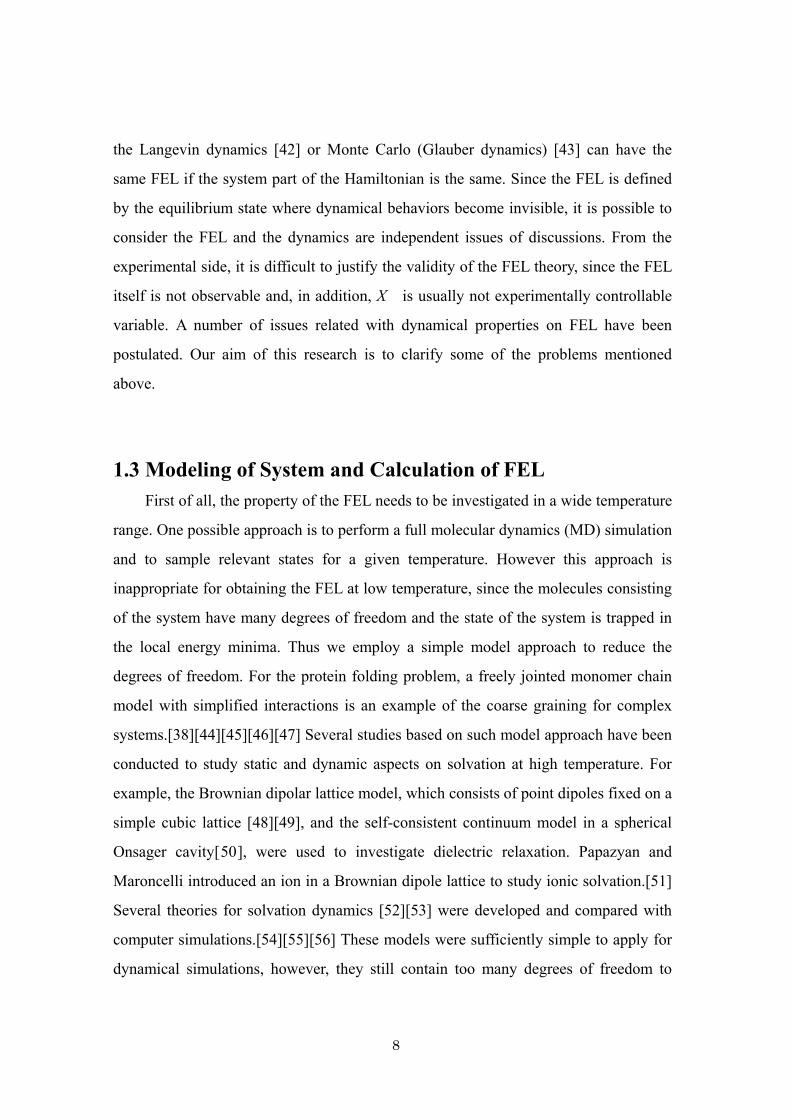
calculate the FELs especially at low temperature. Therefore we take a minimalist

model approach for investigating the FEL, which was originally introduced by

Onuchic and Wolynes to study glassy behavior of solvent molecules in electron and

charge transfer reactions.[57] In this approach, ionic solvation on a polar solvent is

modeled by a central charge surrounded by dipolar molecules with rotational dynamics

represented by dipoles pointing only in two directions, the inward and outward

directions relative to the ion as shown in Fig. 1.1. The simplicity of this model allows

us to thoroughly explore how the energetics of solvation depend on solute charge,

solvent dipole, and number of solvent molecules with an aid of random energy model

(REM) theory, where the interaction energies among solvent molecules were assume to

have a Gaussian distribution independent of the microscopic details of the molecular

interactions.[58][59] Note that the approach based on the REM approximation was

used for the protein folding problem by Bryngelson and Wolynes.[60] The minimalist

model was also applied to investigate the dynamical phase transition [61][62] using

Monte Carlo kinetics in addition to thermodynamic phase transition by utilizing the

(mean) first passage time idea [63]. The extension of the minimalist model to

multilayer solvent molecules with all dipole-dipole and charge-dipole interactions were

applied to investigate the multiple glassy transitions associated with the freezing of the

different solvent layers.[64]

10

q

Figure 1.1: Minimalist model originally introduced by Onuchic and Wolynes. The ionic solvation on a polar solvent is modeled by a central charge surrounded by dipolar molecules with simple rotational dynamics represented by dipoles pointing only in two directions, the inward and outward directions relative to the ion. The translational motion of the surrounding dipoles is omitted and the dipoles are located on a single shell with random displacements.

For large systems, it is not appropriate to generate all states to calculate the FEL,

because the huge number of states exists. Thus the sampling method is suitable,

however it is expected that the state trapping in local minima occurs at low temperature

using the Monte Carlo method with Metropolis algorithm [65] even if the degrees of

freedom decrease. To overcome the difficulty, the generalized-ensemble algorithms

[66] have been developed. The algorithms enable us to sample relevant states even in

the low temperature case by using non-Bortzmann sampling weigh factors. One of the

most well-known generalized-ensemble algorithms might be the multicanonical

algorithm proposed by Berg and Neuhaus.[67][68] The entropic sampling [69][70],

Wang-Landau sampling [71][72] and adaptive umbrella sampling [73] of the potential

energy [74] also refer to the multicanonical algorithm. The generalized-ensemble

algorithm has been applied to many problems such as spin glass, proteins and

polymers.[75][76][77][78] Okumura and Okamoto suggested the multidimensional

11

extensions of the multicanonical algorithm.[79][80] In Chapter 2, we explain the detail

of the Wang-Landau algorithm.

1.4 Multidimensional Spectroscopy For investigating the state dynamics on the FEL, we monitor the dynamics not

only by linear absorption spectroscopy but also by multidimensional spectroscopy.[81]

Since the multidimensional spectroscopy is proven to be a powerful tool for surveying

molecular nature [ 82 ], several theoretical [ 83 ][ 84 ][ 85 ][ 86 ], experimental

[87][88][89][90] and computational [91][92][93][94][95] efforts have been made to

understand the manifold information for molecular motions and interactions. The

multidimensional spectroscopy is the optical counterpart of multidimensional

NMR[96] that can sensitively prove dynamical aspects of molecules in condensed

phases. An observable in multidimensional vibrational spectroscopy is multibody

correlation function of polarizability or dipole moment. The n-body correlation

function is given as

( ) ( ) ( ) ( ) ( )1 2 1 1 2 1, , , , ,nn n n nC t t t V t V t V t V− − − −

⎡ ⎤⎡ ⎤⎡ ⎤⎡ ⎤= ⎣ ⎦⎣ ⎦⎣ ⎦⎣ ⎦ (1.4.1)

where ( )tV is the Heisenberg operator of V and represents the ensemble

average. The operator V is the polarizability and the dipole moment for Raman and

infrared (IR) spectroscopy, respectively. The three-body and four-body correlation

functions are observed in the cases of fifth-order Raman and second-order IR and in

those of seventh-order Raman and third-order IR, respectively. When a particle is

driven by the harmonic potential and interacts with the external filed linearly, the three-

and four-body correlation functions vanish because of the Gaussian integrals involved

in the thermal average or cancellation of the coherence involved in the different

Liouville paths. The multidimensional spectroscopy is sensitive to the anharmonisity

and nonlinearity of system and is one of the available tools for investigating the

microscopic details of the system such as mode-mode coupling [97][98][99][100] and

dephasing mechanisms.[ 101 ][ 102 ][ 103 ][ 104 ][ 105 ] Note that the sensitivity is

12

applicable not only to the kinetic systems following the quantum or classical dynamics,

but also to the non-kinetic systems following the master equation or Smoluchowski

equation.[106] The sensitivity of the multidimensional spectroscopy is fully taken into

account when the dynamics is explored on different FELs.

1.5 Organization of This Thesis In this thesis we introduce three types of models to investigate the properties of

the FEL. In Chapter 2 we analyze a model for representing the ionic solvation which is

the association of dipolar or ionic solvent molecules with a solute ion.[3] The model

consists of a central charge surrounded by dipolar molecules posted on

two-dimensional distorted lattice with simple rotational dynamics. Our interest is the

structure of the FEL especially in the low temperature case. After obtaining the FEL for

the ionic solvation system, we compare the results with the FEL given by employing a

random energy model (REM) approximation.[58][59] We discuss how the structure of

the FEL changes depending on the central charge in a wide temperature range.

In Chapter 3 we consider the FEL for the electron transfer system and introduce a

model consists of a solute dipole surrounded by dipolar molecules with simple

rotational dynamics located on the three-dimensional distorted lattice sites. The

interaction energy between the solute and solvent dipoles as a reaction coordinate is

adopted and the FELs are calculated by generating all possible states for a

26-dipolar-system and by employing the Wang-Landau sampling algorithm for a

92-dipolar-system. For the high temperature case the structure of the FEL is quadratic

form, while for the low temperature case a notched structure appears on the FEL

because of the complex interactions among solvent dipoles. The formation of the

notched structure is analyzed with a statistical approach. The analysis indicates that the

amplitude of the notched structure depend upon the segment size of the reaction

coordinate and characterized by the interaction energy among dipoles. Using the

simulated FEL, we calculate the reaction rates as a function of the energy gap for

13

various temperatures.

In Chapter 4 a general purpose model for investigating the relationship between

the FEL structure and relaxation dynamics is introduced. A dipolar crystal system is

modeled by dipolar molecules posted on two-dimensional lattice sites with two-state

librational dynamics. All dipole-dipole interactions are included to have frustrated

interactions among the dipoles. To relate the FEL to the direct observable quantity, the

reaction coordinate is chosen to be the polarization. For investigating dynamical

aspects of the system, single flip and single-double mixed flips dynamics of dipoles are

incorporated into the model with an aid of a master equation. The first- and third-order

response functions of polarization, which are the observables of linear and

two-dimensional (2D) IR or far IR spectroscopies, are calculated for different

conditions characterized by the FEL. Since the profile of 2D IR spectroscopy is

expected to detect the dynamics hidden in FEL, thus we are able to demonstrate the

different dynamics following the Smoluchowski equation. The validity of the

Smoluchowski equation approach to study the dynamics of system on the calculated

FEL is also examined by calculating 1D and 2D signals to compare with the dynamics

following the master equation.

In Chapter 5, we summarize this thesis and our conclusion is stated.

14

15

Chapter 2 Free Energy Landscape Analysis for Ionic Solvation System

2.1 Introduction Ionic solvation is the process of attraction and association of solvent molecules

with solute ions. Solvation plays an important role in many chemical processes in

condensed phases such as electron and charge transfer reactions.[3][4] Complex

dipolar interactions among solvent molecules cause the energy fluctuation which is

necessary for thermally activated processes. To explore a role of solvation, one

possible theoretical approach is to perform full molecular dynamics (MD) simulations

by placing the charge in a collection of explicit solvent molecules. To have a fairly

complete view of the solvent effect, one has to make an ensemble average over all

possible trajectories of molecular motions. This approach is possible for high

temperature case [ 107 ]; however, it is extremely difficult to apply for a low

temperature case since the solvent molecules have too many degrees of freedom and

there are too many local minima in the free energy landscape (FEL) at low

temperatures. Despite of the complexity of the system, there is a still possibility to

explain a role of solvent using a single macroscopic variable. For example, Marcus

introduced a FEL as a function of a macroscopic variable representing the collective

nature of the solvent molecules.[3] The solvent is treated as homogeneous dielectric

continuum and the FEL is expressed as a quadratic function of the solvent polarization,

which is adopted as the reaction coordinate for representing rearrangements of the

solvent environment. Electron transfer (ET) rates are then evaluated in terms of the

FELs for solvated reactants and products. The advantage of analyzing the system by

means of the FEL is on the inclusion of entropic contributions upon the possible paths

of chemical processes. For example, in electron transfer (ET) and charge transfer (CT)

problems, a reaction rate may be calculated by averaging over all possible reaction

paths with relevant statistical weight [19] [20] [21][22][23][24], since there are infinite

16

numbers of reaction paths due to so many degrees of freedom arise from the solvent

states. This procedure is almost impossible to carry out except for the high temperature

case. The success of Marcus theory indicates that introducing a FEL is indeed an

effective way to describe the reaction processes at least above the freezing temperature.

Since the macroscopic variable may not be sensitive to the microscopic details of the

interactions, we may employ a simple model to gain insight into a role of ionic

solvation. For example, if we separate the rotational and translational degrees of

freedom of solvent molecules, we can simplify the statistical analysis and facilitate

construction of reliable energy landscapes at low temperatures. As mentioned in the

Chapter 1, there are several studies based on such model approach suitable for studying

dynamical aspects of solvation at high temperature, however they still contain too

many degrees of freedom to calculate FELs. For this purpose, we take a minimalist

model approach [57] and calculated the FELs as a function of the polarization.

The organization of this chapter is as follows. In section 2.2, a model composed of

a single charge and dipolar solvent is described. The FEL is introduced as a function of

a collective solvent variable. In section 2.3, the Wang-Landau algorithm is introduced

to calculate the density of states as a function of energy and polarization. The

numerical results are presented in section 2.4, and the final section is devoted to the

conclusion.

2.2 Simulation Model for Ionic Solvation The original minimalist model consists of a charged cavity and a single shell of

solvent molecules represented by dipoles with simple rotational dynamics. These

dipoles were allowed to point only two directions, inward to and outward from the

charged cavity. Tanimura et al. extended the single shell of solvent molecules to two

layers.[64] Monte Carlo simulations were carried out on this system including all

dipole-dipole and charge-dipole interactions. We post the dipoles on a two-dimensional

square lattice having lattice constant L and containing structural disorders (Fig. 2.1).

17

The position of the j th dipole jr can be expressed using a lattice point vector

ja and displacement vector from the lattice point jaδ , i.e., jjj aar δ+= . The

strength and the unit vector specifying the direction of a dipole are μ and

jS respectively, where ||/ jjj rrS = . If we introduce the sign operator 1±=jσ ,

where the sign depends on whether the dipoles are pointing toward or away from the

charge, the dipole movement is expressed as jjSμσ− . Thus, the charge-dipole and

dipole-dipole interactions are explicitly given by

{ }( )1

1 2 1( )

jN N

tot i i i jk j ki j k

E q Jσ ξ σ σ σ−

= = =

= − +∑ ∑∑ , (2.2.1)

where we set

2( )ii

qqrμξ = − , (2.2.2)

and

( )( )2

25

3j k jk j jk k jkjk

jk

J μ⋅ − ⋅ ⋅

=S S r S r S r

r (2.2.3)

with kjjk rrr −= . The system exhibits a glassy behavior at various low temperatures

because of these complex interactions with structural disorder. For the units of

parameters, we employ values typical of ET or CT systems in polar solvents. Thus, q ,

μ and L are chosen to be 0.1 of the electron charge, the unit of Debye, and the unit

of 2.1 A , respectively. Adopting such typical units, the energy unit becomes 201008.1 −× J, which is about 2.5( TkB ) at room temperature. Then, simulations are

carried out for 85.1=μ and 1=L for different q and temperatures. The

displacements from the lattice points obey a Gaussian distribution with average

0=jaδ and standard deviation 1.02 =jaδ . As a collective solvent coordinate,

we introduce the total polarization defined by

p n n− += − (2.2.4)

where +n and −n represent the number of dipoles directed inward to and outward

from the charged cavity, respectively, and the total number of dipoles are given by

N n n− += + . (2.2.5)

18

We further introduce the average polarization per dipole defined by Npx /= . The

FEL is then expressed in terms of x and T as

{ }( )( ){ }

( , ) ln exp /i

Btot i B

x

k TF x T E k TN N σ

σ∈

= − −∑ , (2.2.6)

where the summation is taken over all configurations for which { }( )ixx σ= . Even in

the present model which consists of a charged cavity and 80 dipoles on a 99×

two-dimensional square lattice, there are too many states to enumerate all

configurations in this summation. The procedures for efficiently sampling relevant

states are essential in order to construct the FELs. Our approach is described in the

following section.

q

L

Figure 2.1: Schematic view of the solute and solvent model system. A solute molecule

is represented by a point charge on the center of two-dimensional square lattice.

Solvent molecules are expressed by dipoles located on disordered lattice sites

surrounding the central charge. Each dipole is allowed to direct only two directions,

toward and opposite to the central charge.

19

2.3 Wang-Landau Algorithm The difficulty in evaluating Eq. (2.2.6) arises from the astronomically large

number of states involved in the summation. Fortunately, such large number of states

allows us to employ a statistical treatment. If we obtain a subset of the ensembles that

are the representative of all of the states in the summation in Eq. (2.2.6), we may

evaluate ),( TxF from the subset. The Monte Carlo method with Metropolis

algorithm[65] has been used to generate such representative ensembles, but this

approach is time consuming for a glassy system at low temperature, because the

trajectory of sampled states generated by the Monte Carlo method is easily trapped in

the local energy minima. To overcome this difficulty, Berg and Neuhaus proposed the

multicanonical algorithm [67][68], which has been applied to such problems in spin

glasses, proteins and polymers.[75][76][77][78] The important aspect of this algorithm

is the generation of a uniform sampling of configurations in energy space using

artificial sampling weights instead of the Boltzmann weights. It means that the

algorithm performs a random walk in energy space that allows the system to overcome

energy barriers. From a set of sampling data, one can obtain thermodynamic averages

at arbitrary temperatures and the calculation of the entropy and the free energy, both of

which are associated with the partition function, is possible. Many researchers have

attempted to improve the efficiency of such algorithms.[66][108] Recently an efficient

algorithm for estimating the weight factors was developed by Wang and

Landau.[71][72] This algorithm consists of two steps; the first step is obtaining the

artificial weight factors by recursive updates, which enables us to get a flat histogram

from the uniform sampling data in the energy space and the second step is generating

configurations using such weight factors and calculating physical quantities by

re-weighting probabilities to conform to the Gibbs ensemble. This algorithm is

efficient for evaluating the free energy, but in order to calculate the FEL, which is a

function of the polarization per molecule, an extension is necessary. We use the

two-dimensional Wang-Landau algorithm to obtain the proper weighting factor not

only for the energy space, but also for the polarization space. This algorithm enables us

20

to obtain the FEL for all possible ranges of the polarization at any temperatures.

The outline of our procedure is as follows. First we introduce the weight factor

),( xEg as a function of the energy E and the average polarization per dipole x .

The transition probability from ),( 11 xE to ),( 22 xE is then defined by

( ) 1 11 1 2 2

2 2

( , )( , ) ( , ) min ,1( , )

g E xp E x E xg E x

⎡ ⎤→ = ⎢ ⎥

⎣ ⎦, (2.3.1)

where ),( 11 xE and ),( 22 xE refer to states before and after a single dipole is

flipped. Next we introduce the histogram ),( xEH defined by the number of visits

made to each state ),( xE . If we can make the histogram sufficiently flat using the

transition rule (2.3.1), the density of states ),( xEn will satisfy the following relation

at arbitrary ),( 11 xE and ),( 22 xE :

1 1 1 1

2 2 2 2

( , ) ( , )( , ) ( , )

n E x g E xn E x g E x

= (2.3.2)

To obtain a flat histogram, first we set 1),( =xEg for all possible ranges of energy

and polarization. If the system attains to the states of energy E and polarization x for each time step during the update procedure Eq. (2.3.1), the weight factor is

modified as ),(),( 0 xEgfxEg → where 0f is the modification factor set by

71828.20 ≅= ef . If the transition ),(),( 2211 xExE → is rejected, we also modify the

factor as ),(),( 11011 xEgfxEg → . Iterating this update procedure yields the random

walk in energy and polarization space and the modification of weight factors within the

accuracy of 0f . When the histogram ),( xEH becomes sufficiently flat, we update

the modification factor 0f as 01 ff = and reset the histogram. In practice, it is not

easy to obtain a perfectly flat histogram, thus if ),( xEH for all possible E and x

attains larger than 80% of the averaged value, ),( xEH , we regard the histogram is

flat. This procedure will be repeated for new modification factor if for 1>i with

1−= ii ff . The updating of if enables us to modify the weight factor more finely.

We stop this iteration when 00000001.1<if . After we obtain the weight factors to

satisfy Eq. (2.3.2), we can normalize the density of states ),( xEn using the condition

,

( , ) 2N

E xn E x =∑ . (2.3.3)

21

Substituting Eq. (2.3.2) into (2.3.3) yields

,

( , )( , ) 2( , )

N

E x

g E xn E xg E x

=∑

. (2.3.4)

Finally, from Eq. (2.2.6), we have the expression of the FEL as

( , ) ln ( , ) expB

E B

k TF T x En E xN N k T

⎛ ⎞⎛ ⎞= − −⎜ ⎟⎜ ⎟⎜ ⎟⎝ ⎠⎝ ⎠

∑ . (2.3.5)

In our simulation, we divide the regions of energy [-700,700] and polarization

[-1.0,1.0] into 1401 and 81 segments, respectively. Since the directions of the dipoles

are restricted to point inward to and outward from the central charged cavity, the

periodic boundary conditions are not appropriate for our model. To avoid artificial

errors from the boundary, we have used the open boundary condition. While we study

the effects of the central charge upon the surrounding dipoles, we can suppress the

influence of boundary dipoles by choosing a large lattice. The validity of the model can

be easily checked by changing the lattice size.

2.4 Density of State and Free Energy Landscape Following the procedure in the previous section, we have carried out simulations

of a system composed of a charged cavity and 80 dipoles on the 99×

two-dimensional square lattice with 85.1=μ and 1=L . In order to adjust the lattice

size, we repeated the simulations for the 77× and 1111× lattices and found that the

properties of the FEL do not change qualitatively if the size is larger than 77× . The

displacements from the lattice points obeyed a Gaussian distribution with the average

0=jaδ and the standard deviation 1.02 =jaδ . Using the two-dimensional

Wang-Landau algorithm, we obtained the density of states (DOS) as the function of the

energy E and the polarization x , ),( Exn , for different central charges 0=q and

10 and the temperatures 20=T , 7 and 1. For comparison we also evaluated the

average DOS, ),( Exn , used in the random energy model (REM) theory, where all

22

dipole-dipole and charge-dipole interactions are assumed to have a random Gaussian

distribution function. Although the REM theory assumes the unrealistic interactions

among the molecules, this allows us to obtain a handy analytical expression for a FEL.

The outline of the REM theory is explained in Appendix A. Note that, the theory

may not predict the energy landscape properly at temperatures below the freezing point.

Since a glassy system becomes frozen in low energy states such temperatures, the FEL

has local minima in shape. However, since the theory averages over the local minima,

the landscape is no longer a ragged function.

In order to adapt the REM theory to the simulation model, we set the two sets of

parameters for the zero central charge, q=0, and the strong central charge, q=10. For

the former set, the average charge-dipole interaction is set as 0.0)( =qξ , the

dipole-dipole interaction 05.0−=J , and their standard deviations 0.02 =Δξ and

91.02 =ΔJ , while for the latter, the parameters are set respectively 90.2)( −=qξ ,

05.0−=J , 64.142 =Δξ and 91.02 =ΔJ .

We plot ),(ln Exn in Figs. 2.2(a) and 2.2(b), and ),(ln Exn in Figs. 2.2(c) and

2.2(d) as contour maps for 0=q and 10=q , respectively. In the peak region

denoted by the solid lines, both the simulation and REM for 0=q show symmetrical

profiles, whereas (b) and (d) for 10=q show unsymmetrical ellipsoidal profiles in

the x -direction due to the energy difference between the inner and outer directions of

dipoles arising from the charge-dipole interaction. For the low energy region

0.200−<E , the distributions of ),(ln Exn are always broader than those of

),(ln Exn . This is because, to adapt to the simulation results, we have overestimated

the width of a Gaussian distribution of the interaction energies used in the REM theory.

The energy distribution from the simulation, which is not shown here, is characterized

by the sum of narrower non-Gaussian peaks.

The free energy landscape (FEL) is calculated from Eq. (2.3.5). For comparison

we also have evaluated the FEL for the REM case from

23

( )( ) ( ) ( )

( ) ( )( )( ) ( )

2

REM1/ 2

1 for 2, /

1 2 for

c

c

EE x TS Nx T T xN TF x T N

E x E S Nx T T xN

∗

∗

⎧ ⎛ ⎞Δ− − >⎪ ⎜ ⎟⎪ ⎝ ⎠= ⎨

⎪ −Δ ≤⎪⎩

( )( ) ( )

( ) ( )( )

( )

22 4

REM

2 43/ 2

ln 22 2 12,

3 4 ln 22ln 2 2 24 ln 2 96 ln 2

c

c

E T TT x q x zJ x T T xTNF x T

N EEE x q x zJ x T T xN N N

ξ

ξ

⎧ ⎛ ⎞Δ ⎛ ⎞ ⎛ ⎞− + + + + + + >⎪ ⎜ ⎟ ⎜ ⎟ ⎜ ⎟⎝ ⎠ ⎝ ⎠⎝ ⎠⎪

= ⎨ ⎛ ⎞⎛ ⎞ Δ +Δ⎪ ⎜ ⎟−Δ + + + + + ≤⎜ ⎟⎪ ⎜ ⎟ ⎜ ⎟⎝ ⎠ ⎝ ⎠⎩

(2.4.1)

(2.4.2)

with

( ) 1 1 1 1ln ln2 2 2 2

x x x xS Nx N∗ ⎡ ⎤+ + − −⎛ ⎞ ⎛ ⎞ ⎛ ⎞ ⎛ ⎞= − −⎜ ⎟ ⎜ ⎟ ⎜ ⎟ ⎜ ⎟⎢ ⎥⎝ ⎠ ⎝ ⎠ ⎝ ⎠ ⎝ ⎠⎣ ⎦, (2.4.3)

by using the same parameters for the DOS calculation. (see Appendix A) The average

solvation energy at polarization x and the standard deviation of the solvation energy

are expressed as )(xE and EΔ , respectively. The FELs have two types of forms

above and below a polarization-dependent phase transition temperature )(xTc . Figures

2.3(a)-(c) show the FELs from the simulations (solid line) and the REM (dashed line)

for zero central charge, 0=q . Figures 2.3(d)-(f) show corresponding data for the

strong central charge, 10=q . The temperatures are set at 20=T , 7 and 1, the dotted

lines in Figs. 2.3 represent the fourth-order polynomial fits ∑=

=4

1)(

j

jj xaxF in

addition to a constant term.

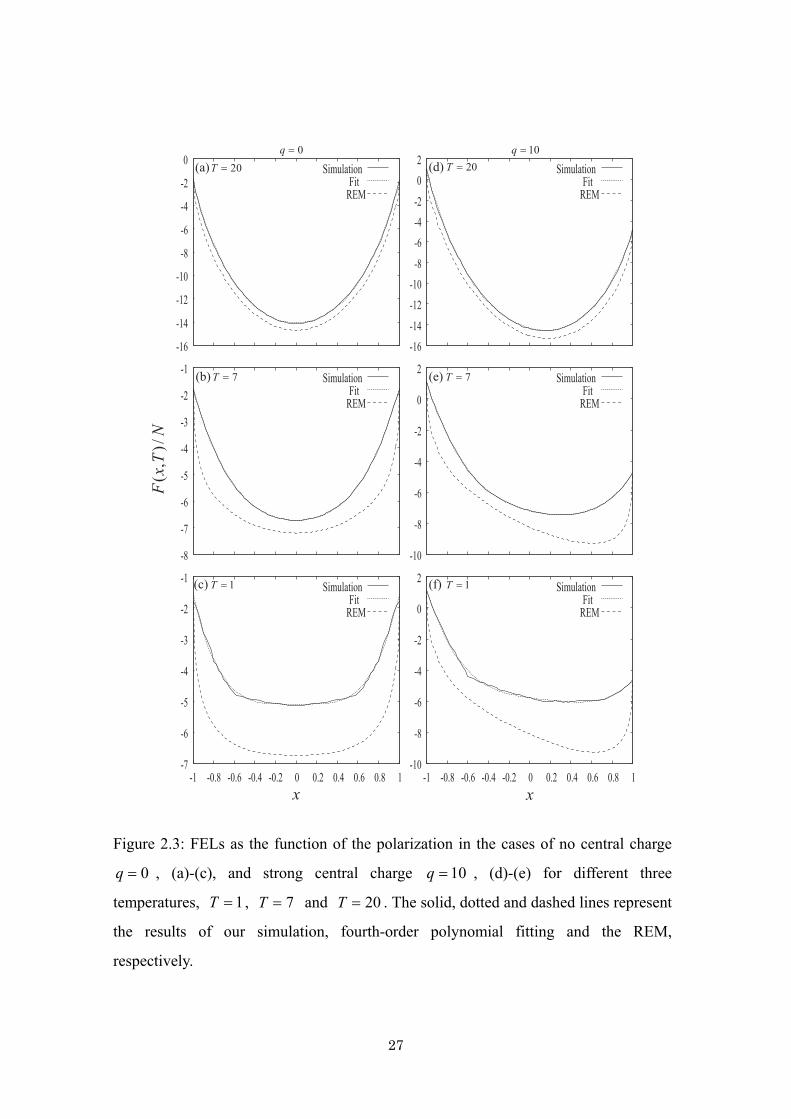
The high temperature case, 20=T is shown in Figs. 2.3(a) and 2.3(d). This

temperature satisfies )(xTT c> for the entire range of x and the REM results

denoted by the dashed lines are calculated only from Eq. (2.4.1). The FEL from the

simulation exhibits a similar profile as REM results. Both curves are parabolic for

small x as predicted by the Born-Marcus theory, but the curvature increases for large

x due to the entropic contribution. In the REM case, this contribution arises from

)(NxTS ∗ in Eq. (2.4.1) where )(NxS ∗ is a logarithmic function of x . To illustrate

the effects of the entropic contribution, we expand ( )REM , /F x T N in Eqs. (2.4.1) and

(2.4.2) for small x as

(2.4.4)

(2.4.5)

where z is the average number of dipoles interacting with each single dipoles.

As can be seen from Eq. (2.4.4), when the temperature becomes high, the

contribution of the second-order coefficient as well as the fourth-order contribution

24

increase. When a strong central charge is present, the dipoles tend to point outward to

decrease the energy. In the case, the term proportional to x in Eq. (2.4.4) also plays a

role in the REM case, the minimum point of landscape shifts to the positive direction.

In the simulation case, there is also a cubic contribution to the FEL. The fitting

function now involves all terms as ∑=

=4

1)(

j

jj xaxF . The lack of the cubic term in the

REM case is due to the oversimplification of charge-dipole interactions. In the

simulation model, the intensity of the charge-dipole interactions change depending on

the location of dipoles, which makes the FEL a complex function of the polarization.

In contrast, the REM theory assumes a spatially uniform interaction which makes the

free energy a linear function of the polarization.

Figs. 2.3(b) and 2.3(e) show the intermediate temperature cases, 7=T . The REM

results in the region of 8.0<x for Fig. 2.3(b) and 6.0<x for Fig. 2.3(e) are

calculated from Eq. (2.4.1) to satisfy )(xTT c> , whereas those in the remaining

regions are calculated from Eq. (2.4.2). The FELs calculated by the REM are broader

than the simulated ones, especially in the region around 1=x and 1−=x . As

illustrated in Fig. 2.2, this can be explained by the fact that a profile of the lower part

of average DOS is always broader because of the overestimation of energy distribution.

In the same manner as in the high temperature case, the FELs can be well fitted by a

polynomial function. As the temperature lowers, the fourth-order contribution of the

fitting curves becomes large as is illustrated by the REM theory. For the fixed

parameter 8.1−=Jz , the ratio 24 / aa in Eq. (2.4.4) increases with decreasing

temperature up to 6.3=T .

Figs. 2.3(c) and 2.3(f) show the results for the low temperature case, 1=T . The

REM results are calculated from Eq. (2.4.2), since this temperature meets )(xTT c<

for the entire range of x . At this very low temperature, the simulated FELs are no

longer smooth due to the presence of multiple local minima arising from the frustrated

interaction among the dipoles. This roughness can be clearly distinguished from the

numerical errors of the simulations, since the errors in these calculations are less than

the line width in Fig. 2.3.

25

Notice that the roughness depends upon the disorder of the dipoles. Thus, if we

make the ensemble average of the FELs for different configurations of dipoles, this

roughness may be smoothed over. On the contrary, the landscape for the REM is

smooth even at the low temperature, since the REM assumes the smooth Gaussian

function for the average DOS.

The profile of the FEL as shown in Fig. 2.3(c) is expressed by a quartic function 4

4)( xaxF ≈ , instead of the parabolic function except for the small roughness of the

lines. On the other hand in Eq. (2.4.5), the contribution of the parabolic term compared

with quartic term is not negligible as 75.0/ 42 =aa for 8.1−=Jz . Thus the quartic

profile of the FEL can not be explained only by the entropic contribution. Since the

dipole-dipole interactions are assumed to be Gaussian random variables, the complex

interactions depending on the position of dipoles are not considered in the REM theory.

Moreover the average energy at polarization x is given by the parabolic form. The

fact that the strong quartic dependence of the FEL is observed at the low temperature

suggests that the average energy contains a quartic term due to the spatial correlation

among dipoles.

Fig. 2.3(f) illustrates the energy landscape for the strong central charge of 10=q .

In addition to the parabolic and quartic contributions of x , the REM case exhibits the

linear contribution, i.e., 44

221)( xaxaxaxF ++≈ , whereas for the simulation case

exhibits the linear and cubic contributions, i.e., 44

33

221)( xaxaxaxaxF +++≈ . As

explained in the Fig. 2.3(d), both the linear and cubic contributions arise from the

charge-dipole interactions. Indeed, they appear even when we calculated the FEL for

the model without the dipole-dipole interactions (not shown).

26

40 30 20 10

-1

-0.5

0

0.5

1

-800 -600 -400 -200 0 200 400 600 800 -800 -600 -400 -200 0 200 400 600 800-1

-0.5

0

0.5

1

0=q 0=q

10=q 10=q

x

x

E E

Simulation REM

(a)

(b)

(c)

(d)

Figure 2.2: Counter maps of the logarithms of the density of states are plotted for the

cases of (a) no central charge 0=q and (b) strong central charge 10=q . For

comparison, the logarithms of the average density of states used in the REM

approximation are also plotted as contour maps for the cases of (c) no central charge

q=0 and (d) strong central charge q=10.

27

-16

-14

-12

-10

-8

-6

-4

-2

0Simulation

FitREM

-8

-7

-6

-5

-4

-3

-2

-1Simulation

FitREM

-7

-6

-5

-4

-3

-2

-1

-1 -0.8 -0.6 -0.4 -0.2 0 0.2 0.4 0.6 0.8 1

SimulationFit

REM

-16-14

-12-10

-8

-6-4-2

0 2

SimulationFit

REM

-10

-8

-6

-4

-2

0

2Simulation

FitREM

-10

-8

-6

-4

-2

0

2

-1 -0.8 -0.6 -0.4 -0.2 0 0.2 0.4 0.6 0.8 1

SimulationFit

REM

(a)

(b)

(c)

(d)

(e)

(f)

20=T

7=T 7=T

1=T 1=T

20=T 0=q 10=q

x x

N

Tx

F/)

,(

Figure 2.3: FELs as the function of the polarization in the cases of no central charge

0=q , (a)-(c), and strong central charge 10=q , (d)-(e) for different three

temperatures, 1=T , 7=T and 20=T . The solid, dotted and dashed lines represent

the results of our simulation, fourth-order polynomial fitting and the REM,

respectively.

28

2.4 Conclusion We calculated the free energy landscape (FEL) as a function of polarization for a

two-dimensional charge-dipole lattice model using the Wang-Landau algorithm. To

elucidate the entropic contributions to the free energy, we supplemented the

calculations using the random energy model (REM) approach by taking the parameters

from the simulation model. In the high temperature case without a central charge, the

FELs calculated from the simulation and REM are parabolic in shape for small

polarizations, as the Born-Marcus theory predicts. In the large polarization region, both

the simulated and the REM results also include a small quartic contribution that arises

from the entropic term in the definition of the free energy as pointed out by Onuchic

and Wolynes.[57]

For the strong central charge, the FEL becomes asymmetric as a result of

charge-dipole interactions. In addition to the quadratic and quartic terms, the FEL is

fitted by linear and cubic terms in the simulation case whereas by a linear term only in

the REM case, because the REM theory oversimplifies the form of the charge-dipole

interactions.

When the temperature decreases, the difference between the simulation and REM

results becomes pronounced. This can be explained more clearly when we plot the

density of states (DOS) as a function of both energy and polarization. The REM results

exhibit a broad DOS due to the overestimation of the interaction energies chosen to

adjust the simulation model to the REM theory. In the low temperature case, the FEL

observed in the simulations is no longer smooth. The roughness arises from the

inhomogeneous charge-dipole and dipole-dipole interactions and depends upon the

positions of the dipoles. By ignoring this roughness, the profile of the FEL is fitted by

a polynomial function up to the fourth-order of the polarization. As in the high

temperature case, the linear and cubic contributions appear when the strong central

charge is introduced.

In this Chapter we have calculated the FELs for a system composed of a charged

cavity and dipoles which are restricted to point only to two directions. The present

29

model is too simple to describe many important effects involved in solvation dynamics,

such as librational motion. Generalization to a realistic model with the large degrees of

freedom in three-dimensional space is necessary to explore the universality of our

results. Thermal as well as dynamical aspects of such system are important to relate the

FEL to real experiments of a relaxation.

30

31

Chapter 3 Free Energy Landscape Analysis for Electron Transfer System

3.1 Introduction The free energy landscape (FEL) of electron transfer (ET) system is of

fundamental importance to account for ET rates in solvent as recognized by

Marcus.[3][4] In this context, the FELs of the reactant and product are expressed in

terms of a reaction coordinate consisting of reactant and product along with their

surrounding of solvent. Marcus evaluated the free energy of a given polarization and

calculated the ET reaction rates as

( )2

exp4 B

Gk

k Tλ + Δ

−λ

⎛ ⎞⎜ ⎟⎜ ⎟⎝ ⎠

∼ (3.1.1)

where λ and GΔ− are the reorganization energy and the energy gap, respectively.

From the above expression, the energy gap law, Marcus has predicted that the inverted

parabolic or bell-shaped dependence of ET rates as the function of energy gap, which

indicates the ET rates increase in the small energy gap region (the normal region),

whereas they decrease in the large energy gap region (the inverted region). His

expression was based on a continuum dielectric model of solvent and thus the

molecular aspects of the solvent were missing.

Although Marcus’s theory explained the energy gap dependence reasonably well

[14][15][16], such macroscopic continuum model is not sufficient to describe ET

processes especially for dynamics of solvent.[109] The FELs of the macroscopic

dielectric system were given by a functional form of polarization.[4][110] To calculate

the FELs using models based on the microscopic molecular details, one has to define

relevant reaction coordinates. Taking statistical mechanics approach, Marcus has

explored ways to abstract small dimensional coordinates from the multidimensional

phase space using the technique of equivalent equilibrium distribution.[111] His idea

was later developed and utilized for the calculation of the ET rate by computer

32

simulations.[112] Calef and Wolynes showed that a reaction coordinate could be

adequately defined by the microscopic interaction energy [17][18], and several

computer simulations were carried out using the reaction coordinate which has the

energy dimension to confirm the legitimacy of Marcus’s theory.[21][22][23][24] An

expression of the free energy in terms of molecular distribution function including

dipole interactions was also given by using a density functional theory.[113][114]

Here, we introduce a factor { }( )iRf for configuration coordinates of solvent

{ }iR as

{ }( ) { }( ) { }( )R Pi i if R E R E R≡ − , (3.1.2)

where { }( ) { }( ) { }( )i i ii d s i s s iE R E R E R− −≡ + is the interaction energy for reactant

( i R= ) or product ( i P= ) consisting the solvent-solute interaction energy,

{ }( )id s iE R− , and solvent dipole-dipole energy { }( )i

s s iE R− .[19][20] If we define the

FELs of reactant and product by

( ) { }( )( ) { }( )( )( )1, ln exp /i iB N i i BG x T k T dR dR x f R E R k Tδ= − − −∫ , (3.1.3)

the free energies of the reactant and the product satisfy the relation,

( , ) ( , )R PG x T x G x T= + . (3.1.4)

Suppose if the FEL is expressed in a quadratic form as

2( , )RG x T ax bx= + , (3.1.5)

the ET rates are then evaluated as Eq.(3.1.1), in which G−Δ is the energy gap

between the two surfaces and a4/1=λ .

At present, the FEL for ET processes is fairly understood at least for the

high-temperature case, where the FEL is well approximated by the parabolic function.

At low temperature, however, it is difficult to calculate the reaction rates, since the

solvent molecules have enormous degrees of freedom and there are too many local

minima that trap molecular motions to acquire the reliable FELs. In order to deal with

such problem, a simple model is often introduced to reduce the degrees of freedom as

33

mentioned in Chapter 1. To study a possible role of solvent molecules influencing the

electron transfer (ET) or charge transfer (CT) reaction rates in glassy phase, we have

utilized the minimalist model approach.[57]

In this chapter, a survey of the FELs for the extended minimalist model as the

function of x defined by Eqs. (3.1.2) and (3.1.3) at temperatures below and above the

freezing point. In Sec. 3.2, we describe the model and the reaction coordinate. In Sec.

3.3, the FELs for different temperatures are numerically calculated by generating all

possible states for a 26-dipolar-system and by employing Wang-Landau sampling

algorithm for a 92-dipolar-system. From the calculated FELs, the ET reaction rates are

also evaluated. The final section is devoted to the conclusion.

3.2 Simulation Model and Reaction Coordinate To adapt minimalist model for ET reaction process, we have replaced the central

charged cavity by a solute dipole moment. Then we configure the solvent dipoles

around the solute dipole on the three-dimensional distorted lattice with the lattice

constant L . We have treated all solute-solvent and solvent-solvent interactions

explicitly, whereas they were assumed to be random Gaussian interactions in the

original minimalist model with the random energy model (REM) analysis. The

schematic view of our modified model is depicted in Fig. 3.1. The solute dipole

moment is represented by idμz , where z is the unit vector in the z direction and i

dμ

denotes the magnitude of the solute dipole for the reactant ( i R= ) and the product

( i P= ). We denote the position of each solvent dipole as jjj aar δ+= , where ja is

the j th lattice point vector and jaδ is the random displacement from the lattice

point. The magnitude and the direction of the jth solvent dipole is denoted by solvμ

and the unit vector jS , respectively, where ||/ jjj rrS = . If we introduce the sign

operator 1±=jσ , where the sign depends on whether the dipoles are pointing toward

or away from the solute dipole, the dipole movement is expressed as solv j jμ σ− S . Thus

all the interactions among solute and solvent dipoles are expressed as

34

( ) ( ) ( ), ,i i i id d s d s sE E Eμ μ− −= +σ σ σ . (3.2.1)

Here, the energy of the solute-solvent and the solvent-solvent dipoles are defined by

( ) ( )1

,N

i i id s d j d j

jE gμ μ σ−

=

= ∑σ (3.2.2)

and

( )1

2 1

N j

s s jk j kj k

E h σ σ−

−= =

= ∑∑σ , (3.2.3)

respectively, where

( ) ( )( )2

5

3j j j j ji ij d solv d

j

g μ μ μ⋅ − ⋅ ⋅

= −S z r S r z r

r (3.2.4)

and

( )( )22

5

3j k jk j jk k jkjk solv

jk

h μ⋅ − ⋅ ⋅

=S S r S r S r

r (3.2.5)

with kjjk rrr −= , and N is the total number of solvent dipoles This system exhibits

a glassy behavior at the low temperatures because of the complex interactions among

the solvent dipoles with the structural disorder. We chose values typical of ET or CT

systems in polar solvents as 85.1=solvμ and 1=L in the unit of Debye and the unit

of 2.1 A , respectively. The characteristic energy is then evaluated as 201008.1 −×=ΔU

J, which is about 2.5( TkB ) at room temperature. We employ two types of system: one

is 333 ×× lattice sites and the other is 5 5 5× × lattice, but we omit four dipoles on

each corner of the lattice for later system due to the limitation of our CPU power. Thus,

we used a total of 26 and 92 dipoles for their calculations. We utilize the open

boundary condition to avoid undesired effects arise from the treatment of boundary.

The displacements from the lattice points obey a Gaussian distribution with average

0=jaδ and standard deviation 1.02 =jaδ .

For our model, we rewrite Eq. (3.1.2) as

( ) ( ) ( ), ,R R P Pd df E Eμ μ= −σ σ σ . (3.2.6)

35

The FELs of the reactant ( i R= ) and the product ( i P= ) are calculated from

( ) ( )( )| |

,1, ln expi i

diB

f x x B

EG x T k T

C k T− <Δ

⎛ ⎞μ⎜ ⎟= − −⎜ ⎟⎝ ⎠

∑σ

σ. (3.2.7)

Here, the summation has taken over all configurations for which ( )σf takes a value

between 2/xx Δ− and 2/xx Δ+ , where xΔ is the segment (mesh) size of the

reaction coordinate. We introduce the dimensionless constant C to adjust the position

of ( )TxG i , . When we set C to be proportional to xΔ , the position of the energy

landscape of various segment sizes can be fixed if the assigned temperatures are the

same. In the following calculations, we set UxC ΔΔ= / , where 201008.1 −×=ΔU J is

the characteristic energy of the system. In Eq. (3.2.7), we adopt 0=Rdμ and 2=P

dμ

for a situation: a neutral solute is surrounded by the solvent in the reactant state and the

ET reaction occurs then is polarized.

For the 26-dipolar-case, we evaluate Eq. (3.2.7) by generating all configurations

of σ and classifying ( )σf in the range ( )/ 2 / 2i ix x f x x− Δ ≤ < + Δσ for ith

segment ix , which satisfies ii xxx −=Δ +1 . Although we can obtain the exact FEL for

any xΔ in such small system, we cannot generate all configurations by any means for

a large system. For example, a system with 92 dipoles involves enormous degrees of

freedom even with directional restrictions of the dipoles ( 922∼ ). Thus, it is essential to

sample relevant states for constructing the FEL, and then to use the Wang-Landau

algorithm explained in Chapter 2. We employ the reaction coordinate x defined in

Eqs. (3.2.6) and (3.2.7) instead of the polarization and adapt the two-dimensional

Wang-Landau algorithm to calculate the FEL. The parameters or conditions used in the

algorithm are shown as follows.

When the histogram ),( xEH defined by the number of sampled states ( )xE,

attains larger than 70% of the average value, ),( xEH , for all possible ranges, we

regard the sampling as having been done uniformly in the energy and reaction

coordinate space. In order to generate the sampling weight, we divide the regions of

energy -2000< /E UΔ <2000 and reaction coordinate -100< /x UΔ <100 into 4001

36

and ( ) 1/200 +ΔΔ xU segments, respectively. We generate the density of states (DOS)

after obtaining the artificial weight factors by recursive updates which enables us to

obtain a flat histogram of the uniform sampling data in the energy and reaction

coordinate spaces. We then calculate the FEL as the function of x by re-weighting

probabilities to conform to the Gibbs ensemble.

Figure 3.1: A schematic view of a solute and solvent model. A solute molecule is

represented by a dipole on the center of three-dimensional square lattice. Solvent

molecules are expressed by dipoles located on the disordered lattice sites surrounding

the central dipoles. Each solvent dipole is allowed to direct only two directions, toward

and opposite to the central dipole.

37

3.3 Results and Discussion A. Free Energy Landscapes of a 26-Dipolar-System

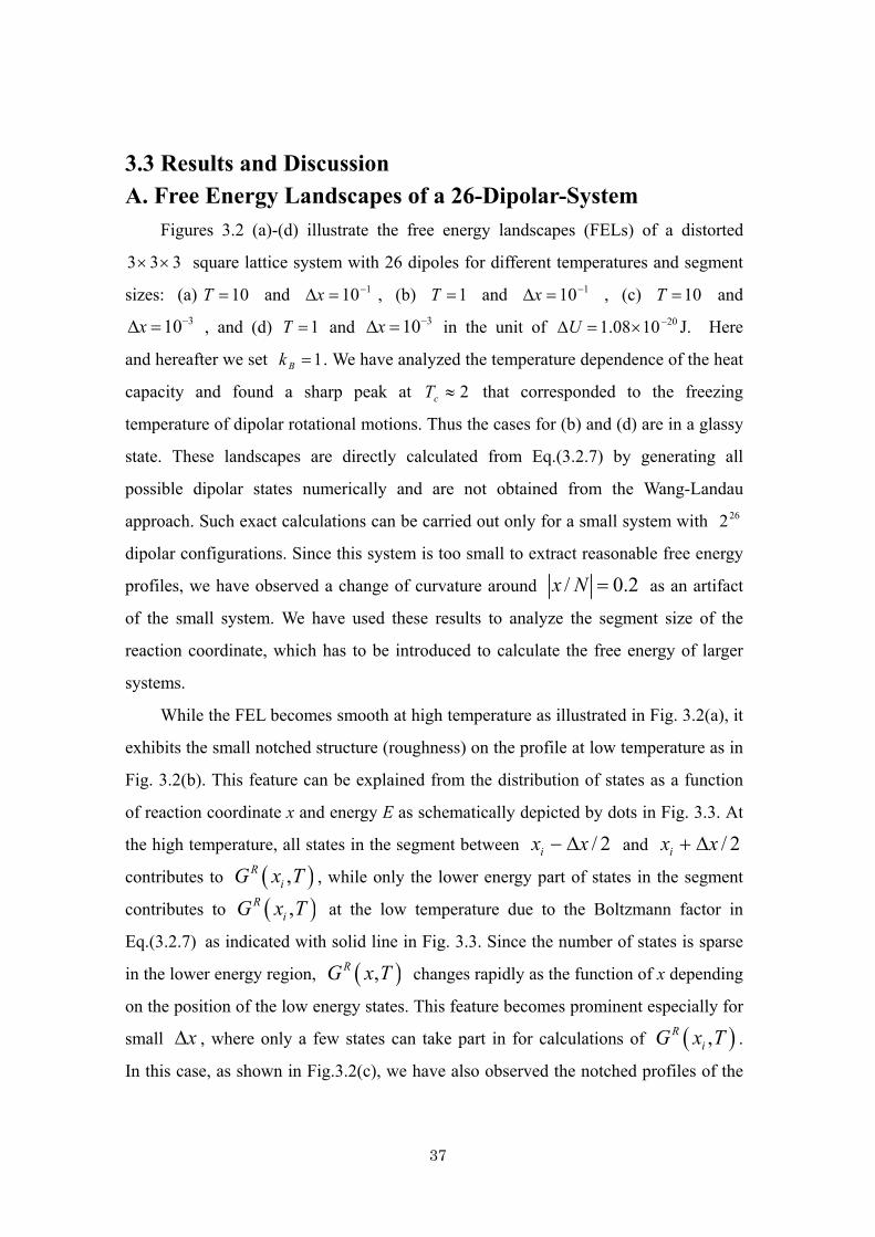
Figures 3.2 (a)-(d) illustrate the free energy landscapes (FELs) of a distorted

333 ×× square lattice system with 26 dipoles for different temperatures and segment

sizes: (a) 10=T and 110−=Δx , (b) 1=T and 110−=Δx , (c) 10=T and 310−=Δx , and (d) 1=T and 310−=Δx in the unit of 201008.1 −×=ΔU J. Here

and hereafter we set 1=Bk . We have analyzed the temperature dependence of the heat

capacity and found a sharp peak at 2≈cT that corresponded to the freezing

temperature of dipolar rotational motions. Thus the cases for (b) and (d) are in a glassy

state. These landscapes are directly calculated from Eq.(3.2.7) by generating all

possible dipolar states numerically and are not obtained from the Wang-Landau

approach. Such exact calculations can be carried out only for a small system with 262

dipolar configurations. Since this system is too small to extract reasonable free energy

profiles, we have observed a change of curvature around / 0.2x N = as an artifact

of the small system. We have used these results to analyze the segment size of the

reaction coordinate, which has to be introduced to calculate the free energy of larger

systems.

While the FEL becomes smooth at high temperature as illustrated in Fig. 3.2(a), it

exhibits the small notched structure (roughness) on the profile at low temperature as in

Fig. 3.2(b). This feature can be explained from the distribution of states as a function

of reaction coordinate x and energy E as schematically depicted by dots in Fig. 3.3. At

the high temperature, all states in the segment between / 2ix x− Δ and / 2ix x+ Δ

contributes to ( ),RiG x T , while only the lower energy part of states in the segment

contributes to ( ),RiG x T at the low temperature due to the Boltzmann factor in

Eq.(3.2.7) as indicated with solid line in Fig. 3.3. Since the number of states is sparse

in the lower energy region, ( ),RG x T changes rapidly as the function of x depending

on the position of the low energy states. This feature becomes prominent especially for

small xΔ , where only a few states can take part in for calculations of ( ),RiG x T .

In this case, as shown in Fig.3.2(c), we have also observed the notched profiles of the

38

landscape even at the high temperature.

Using the exact distribution of states, we analyzed the statistics of the notched

structure. First, we extrapolate the profiles of the FEL up to sixth-order using the

fitting function ( ) ( )∑=

=3

0

2/k

ki

Rfit NxaxG for the range 2.0/ ≤Nx . Due to the

conditions of ( ) ( )σσ −−= ff and ( ) ( )σσ −= ,, Rd

RRd

R EE μμ , ( ),RG x T is

symmetric with respect to 0=x and the polynomial function does not contain the

odd-order terms. Then we subtract ( )xG Rfit from NTxG R /),( and obtain the

notched part of free energy as ( ) ( ) ( )iRfiti

Ri xGNTxGxG −= /,δ , where ix is the

value of the reaction coordinate at ith segment which satisfies ii xxx −=Δ +1 .

NTxG R /),( for 1=T and 210−=Δx is depicted in Fig. 3.4 with solid line and the

fitted line is with the dashed line, in which the fitting parameters are 75.67316 =a ,

4 307a = − , 2 3.9a = and 0 2.26a = − . The inset of Fig. 3.4 shows the histogram of

( )iG xδ and the fitted normal distribution with dashed line where the average and the

standard deviation are 0.0=Gδ and 098.02 =Gδ , respectively. In the small

region of x, where the Gaussian fitting works well, the sequence of ( )ixGδ is

uncorrelated at the different 'ix and thus ( )ixGδ can be regarded as the white noise

with respect to ix .

Calculated 2Gδ as the function of temperature for different xΔ is plotted in

Fig. 3.5. The amplitude 2Gδ tends to be large for small xΔ , since the number of

the states involved in the free energy calculations becomes small and the statistical

deviation becomes large. For 10T < , the amplitude becomes large for small T ,

since only lower energy states in the segment can contribute to the free energy

calculations due to the Boltzmann factor in Eq. (3.2.7). At very low T , the lowest

energy state in the segment dominate the free energy and thus we have

( ) min,Ri iG x T E≈ , where min

iE is the lowest energy in the ith segment and therefore

the FELs becomes temperature independent. For 10>T , 2Gδ increases as the

temperature increases. At such high temperature, the Boltzmann factor play a lesser

role and thus the total number of states, n(xi), in the ith segment determines the value

of the free energy as )(ln iB xnTk− . Since n(xi) may change rapidly for small xΔ , the

39

amplitude will also change.

In Fig. 3.6, we plot UG Δ/2δ as the function of Ux ΔΔ / for different

temperatures, where UΔ is the characteristic energy scale for the system. The

calculated results can be well fitted by the linear functions in the logarithmic scales.

This indicates that we can always extrapolate their amplitudes 2Gδ from the values

in large xΔ .

Since the lowest energy miniE determines the free energy in the individual

segments especially for the low temperature case, the differences of the lowest energy

among the different segments give rise to the notched structure. To see this point more

clearly, we consider the change of the total energy and the reaction coordinate by

flipping one dipole while others being fixed. The energy of the k th dipole is evaluated

as

( ) 2

2

k k kj k jj k

k jj k

E h

h≠

≠

Δ σ → −σ = − σ σ

≈ − σ σ

∑

∑, (3.3.1)

where the interaction parameter kjh is approximated by their mean value h defined

by

1

1 11

N

kjk j k

h hN N= ≠

⎛ ⎞≡ ⎜ ⎟−⎝ ⎠

∑ ∑ . (3.3.2)

Similarly, the change of the reaction coordinate by flipping one dipole is given by

( ) ( )2

2

Pk k k d k

k

x g

g

Δ σ →−σ = μ σ

≈ σ, (3.3.3)

where the solute-solvent interaction parameter ( )Pdkg μ is approximated by their mean

value

( )1

1 NP

k dk

g gN

μ=

= ∑ . (3.3.4)

If all configurations of { }Nkk σσσσ ,,,, 111 +− occur with the same probability, 12/1 −N , the fluctuation (standard deviation) of the total energy and reaction coordinate

40

by flipping one dipole are given by

( )2 1flipE h NΔ = − , (3.3.5)

and

2flipx gΔ = , (3.3.6)

respectively. For the 26-dipolar-system, they are evaluated as 0.9h = and 0.05g = ,

and we have 0.1flipxΔ = and / 0.3flipE NΔ = . These values are roughly in

accordance with the relation in Fig. 3.6, which indicates that the amplitude of the

notched structures relates to the flipping energy and the corresponding change of the

reaction coordinate. We should also notice that although the true FELs have the

notched structures whose scale is much smaller than flipxΔ , a real transition may

occur only through the flipping of dipoles. Therefore the structure smaller than flipxΔ

on the FELs may not affect reaction processes.

41

Figure 3.2: The free energy landscapes of a distorted 333 ×× square lattice system

with 26 dipoles for different temperatures T and segment sizes xΔ : (a) 10=T and 110−=Δx , (b) 1=T and 110−=Δx , (c) 10=T and 310−=Δx , and (d) 1=T and 310−=Δx . T and xΔ are measured in the unit of 201008.1 −×=ΔU J and we set

1Bk = .

42

Δx

x

E

xi

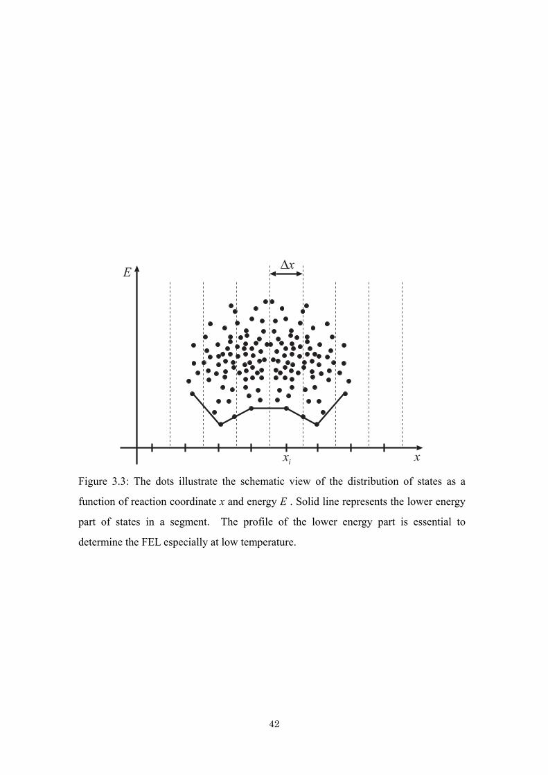
Figure 3.3: The dots illustrate the schematic view of the distribution of states as a

function of reaction coordinate x and energy E . Solid line represents the lower energy

part of states in a segment. The profile of the lower energy part is essential to

determine the FEL especially at low temperature.

43

-2.8

-2.6

-2.4

-2.2

-2

-1.8

-1.6

-1.4

-0.2 -0.15 -0.1 -0.05 0 0.05 0.1 0.15 0.2

0

0.01

0.02

0.03

0.04

0.05

0.06

-0.6 -0.4 -0.2 0 0.2 0.4 0.6Deviation from fitting curve

Nor

mal

ized

dis

tribu

tion

x N/

Gx

TN

R,

/(

)

×( )ΔU

×( )ΔU

Figure 3.4: The free energy landscape (solid line) and fitted curve (dashed line) of a

distorted 333 ×× lattice model for 1=T and 210−=Δx . The fitting function is

( ) ( )∑=

=3

0

2/k

ki

Rfit NxaxG with parameters 75.67316 =a , 4 307a = − , 2 3.9a = and

0 2.26a = − . The inset of the figure shows the histogram of ( )iG xδ , which is fitted by

the normal distribution (dashed line) with the average 0.0=Gδ and the standard

deviation 098.02 =Gδ .

44

0

0.02

0.04

0.06

0.08

0.1

0.12

0.14

0.16

0 5 10 15 20 25 30 35 40 45 50

Δx =1Δx = −10 1

Δx = −10 2

Δx = −10 3

Δx = −10 4

δG2

T

×( )ΔU

×( )ΔU

Figure 3.5: The standard deviation 2Gδ for the 26-dipolar-system as the function of

the temperature for various segment sizes.

45

-9

-8

-7

-6

-5

-4

-3

-2

-1

-4 -3 -2 -1 0

T =1T = 5T =10

log /Δ Δx U

ln/

δGU

2Δ

Figure 3.6: The standard deviation UG Δ/2δ for the 26-dipolar-system as the

function of the segment size Ux ΔΔ / , where UΔ is the characteristic energy scale of

the system. The calculated results can be well fitted by the linear functions in the

logarithmic scales.

46

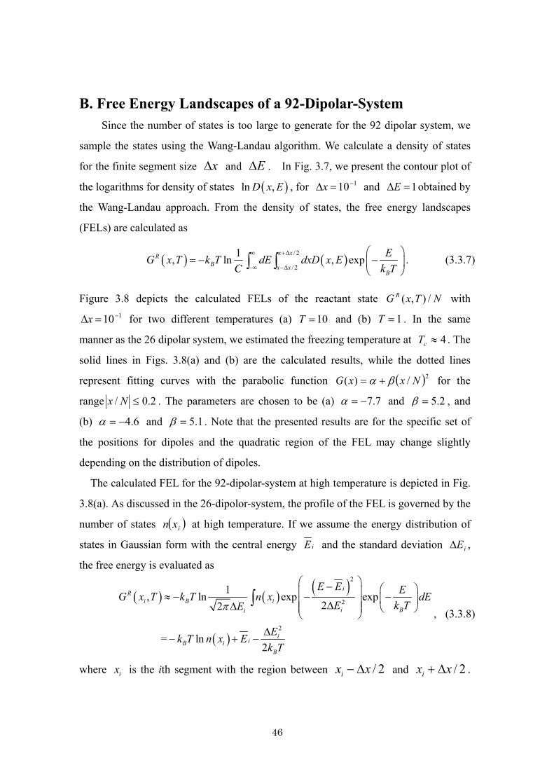
B. Free Energy Landscapes of a 92-Dipolar-System Since the number of states is too large to generate for the 92 dipolar system, we

sample the states using the Wang-Landau algorithm. We calculate a density of states

for the finite segment size xΔ and EΔ . In Fig. 3.7, we present the contour plot of

the logarithms for density of states ( )ln ,D x E , for 110−=Δx and 1=ΔE obtained by

the Wang-Landau approach. From the density of states, the free energy landscapes

(FELs) are calculated as

( ) ( )/ 2

/ 2

1, ln , expx xR

B x xB

EG x T k T dE dxD x EC k T

∞ +Δ

−∞ −Δ

⎛ ⎞= − −⎜ ⎟

⎝ ⎠∫ ∫ . (3.3.7)

Figure 3.8 depicts the calculated FELs of the reactant state NTxG R /),( with 110−=Δx for two different temperatures (a) 10=T and (b) 1=T . In the same

manner as the 26 dipolar system, we estimated the freezing temperature at 4≈cT . The

solid lines in Figs. 3.8(a) and (b) are the calculated results, while the dotted lines

represent fitting curves with the parabolic function ( )2/)( NxxG βα += for the

range 2.0/ ≤Nx . The parameters are chosen to be (a) 7.7α = − and 5.2β = , and

(b) 4.6α = − and 5.1β = . Note that the presented results are for the specific set of

the positions for dipoles and the quadratic region of the FEL may change slightly

depending on the distribution of dipoles.

The calculated FEL for the 92-dipolar-system at high temperature is depicted in Fig.

3.8(a). As discussed in the 26-dipolor-system, the profile of the FEL is governed by the

number of states ( )ixn at high temperature. If we assume the energy distribution of

states in Gaussian form with the central energy iE and the standard deviation iEΔ ,

the free energy is evaluated as

( ) ( )

( )

( )

2

2

2

1, ln exp exp22

= ln2

iR

i B ii Bi

iiB i

B

E E EG x T k T n x dEE k TE

Ek T n x Ek T

π

⎛ ⎞− ⎛ ⎞⎜ ⎟≈ − − −⎜ ⎟⎜ ⎟ΔΔ ⎜ ⎟ ⎝ ⎠⎝ ⎠

Δ− + −

∫, (3.3.8)

where ix is the ith segment with the region between / 2ix x− Δ and / 2ix x+ Δ .

47

Near the minimum of free energy surfaces 2.0/ ≤Nx , since a large number of states

are involved in ( )n x , we can assume Gaussian form for ( )n x based on the central

limiting theorem. For the high temperature case, the contribution from ( )lnB ik T n x−

is large and therefore we have the parabolic energy landscapes for 2.0/ ≤Nx . For

large Nx / , however, )(xn contains only a small number of states and deviates

from Gaussian due to the failure of the central limiting theorem. (See also Fig. 3.7).

Consequently, ),( ExG R shows parabolic and non-parabolic profiles for small and

large Nx / , respectively. We should notice, however, that although such feature

exists for any system, the deviation from the parabola may be too small to observe in a

real system, since it contains tremendous degrees of freedom that makes the deviation

very small.

Figure 3.8(b) shows the FEL for 1=T . In the low temperature case, FELs are

determined by the lower energy part of distribution D(x, E), because the Boltzmann

weight in Eq.(3.3.7) suppress the higher energy contributions. Since the lower energy

part of D(x, E) is not a smooth function of x as illustrated in Fig. 3.7, the calculated

FELs at low temperature exhibit the notched structure as presented in Fig. 3.8 (b).

Following the same procedure as the 26-dipolar-system, we have extracted the notched

part ( )xGδ for all ranges of x and analyzed their statistics. The amplitude of the

notched part of profiles 2Gδ changes depending upon the size of xΔ . Due to the

limitation of CPU power; however, we can calculate the values of 2Gδ for low

temperature 1=T only for relatively large segments, i.e. 1.0=Δx , 5.0 and 1 .

Thus, by assuming the relation between xΔ and 2Gδ found in 3.3.A, here we

have extrapolated the value of 2Gδ for small xΔ and found

87.2/log15.0/ln 2 −ΔΔ−=Δ UxUGδ . This relation is in accordance with the

change of the total energy and the reaction coordinate by flipping one dipole

represented by /flipE NΔ and flipxΔ . In the 92-dipolar-system, we estimate the

average solute-solute and solute-solvent interaction energies as 0.27h = and

0.01g = − , respectively, and therefore we have 0.02flipxΔ = and

/ 0.06flipE NΔ = . From the extrapolated function, we have 2 0.07Gδ = if we

48

regard flipxΔ as the segment size. This value is roughly in accordance with

/flipE NΔ , which indicates the changes of energy for flipping dipoles are reflecting

the amplitude 2Gδ .

For a system with large degrees of freedom, the minimal values of xΔ can be very

small, but, the energy landscape with the segment size flipx xΔ ≈ Δ is of practical

importance for reaction process as mentioned in 3.3.A.

-60 -40 -20 0 20 40 60-600

-400

-200

0

200

400

600

800

1000

1200 50 40 30 20 10 0

x

E

×( )ΔU

×( )ΔU

Figure 3.7: The contour plot of the logarithms of the density of states, ( )ln ,D x E , for

the 92-dipolar-system. The segment sizes for the reaction coordinate and energy are

chosen to be 110−=Δx and 1=ΔE , respectively. The density of states is obtained

by the Wang-Landau approach.

49

-8-7-6-5-4-3-2-1 0 1 2

-0.6 -0.4 -0.2 0 0.2 0.4 0.6

Fitting curve

-5

-4

-3

-2

-1

0

1

2

3

-0.6 -0.4 -0.2 0 0.2 0.4 0.6

Fittig curveT =1

T =10(a)

(b)

x N/

Gx

TN

R,

/(

)G

xT

NR

,/

()

×( )ΔU

×( )ΔU

×( )ΔU

Figure 3.8: The calculated free energy landscapes for the 92 dipolar system

NTxG R /),( with 110−=Δx for different temperatures (a) 10=T and (b) 1=T ,

respectively.

50

C. Energy Gap Low for ET Reaction Rates The FEL for ( )TxG P , is obtained from ( ),RG x T by using Eq. (3.1.4). Using

the energy landscapes for the 92-dipolar-system, we calculate the activation energy

G≠Δ as the function of energy gap GΔ . If we denote the minimum values of the

reactant and product states as RGmin and PGmin , respectively, and express the crossing

point of the two surfaces as x≠ , we have

( ) ( )min min, ,R R P PG x T G G x T G G≠ ≠− = − + Δ (3.3.9)

which allows us to calculate x≠ for fixed GΔ . Since the activation energy G≠Δ is

given by

( ){ }min,R RG G x T G≠ ≠Δ = − , (3.3.10)

we can depict the energy gap law by plotting ≠Δ− G as the function of GΔ− .

Figure 3.9 shows the energy gap dependence of the activation energy at the

temperatures 10=T (dashed line) and 1=T (solid line) calculated from the energy

landscapes with the segment size 1.0=Δx , which is slightly larger than flipxΔ . All

curves of the activation energy are symmetric with respect to the maximum point,

since the FEL for the reactant states is the even function. In the low temperature case,

1=T , the energy gap law exhibits roughness reflected on the notched structure of the

energy landscape. Although the profiles of the roughness may change depending upon

xΔ , the segment size smaller than flipxΔ is not necessary to consider the reaction

processes because the states can only change through the dipolar flipping in the order

of flipxΔ . Notice that the microscopic profiles of the roughness differ depending on

the distribution of the dipolar positions and if we take an ensemble average for

different distributions, such small roughness on the activation energy may not be

observed.

Due to the non-parabolic shape of energy landscapes, the energy landscapes are

not quadratic besides small | x |. The calculated energy gap decreases faster than the

quadratic function besides the range about 0.2GΔ ≤ . This deviation becomes large

51

for high temperature case, since the FEL becomes steep as explained by Eq.(3.3.8).

The energy gap low, Eq. (3.1.1), indicates the maximum reaction rate depends on

the reorganization energy λ . When a temperature rises, the profile of activation

energy also shifts to the left for 10T ≥ as illustrate in Fig. 3.10. For high temperature

case, the FEL can be written as ( ) ( ), lnRBG x T k T n x≈ − . Since ( )n x is

approximated by a temperature-independent Gaussian function for small x , we can

express the free energy as

2

min1( , )

2P PG x T aT x G

aT⎛ ⎞= − +⎜ ⎟⎝ ⎠

(3.3.11)

where a is some constant and minPG satisfies min min 1/ 4P RG G aT= − . Since the

crossing point and the activation energy are expressed as 1/ 4x G aT≠ = Δ + and

( ) ( )( )

( )

2

4G T

GTλ

λ≠

−Δ −−Δ = − , (3.3.12)

respectively, the peak position of the activation energy is equal to the reorganization

energy ( ) 1/ 4T aTλ = . The peak positions of the calculated results are plotted in Fig.

3.10. These results are well fitted by ( ) 1/ 4T aTλ = with 34.9 10a −= × as illustrated

by the solid line in the figure. For studying the solvation saturation effect, Milischuk

and Matyushov utilized the relation that the reorganization energy is proportional to

1/T for a dipolar solvation system at constant volume.[115] The present results are

consistent with their analysis.

52

-1.2

-1

-0.8

-0.6

-0.4

-0.2

0

-0.4 -0.3 -0.2 -0.1 0 0.1 0.2 0.3 0.4 0.5

T =1T =10

−≠

ΔGN/

−ΔG N/ ×( )ΔU

×( )ΔU

Figure 3.9: The energy gap dependence of the activation energy at the temperatures

10T = (dashed line) and 1T = (solid line) calculated from the energy landscapes

with 0.1xΔ = .

53

0

0.01

0.02

0.03

0.04

0.05

0.06

10 20 30 40 50 60 70 80

SimulationFitting curve

−(

)ΔG

TN

0/

T

×( )ΔU

Figure 3.10: The reorganization energy, ( )Tλ , which gives the minimum activation

energy is plotted for different temperatures for 10≥T (dots). The solid line

represents the fitting curve, ( ) 1/ 4T aTλ = , with 3109.4 −×=a .

54

3.4 Conclusion We calculated the free energy landscape (FEL) by generating all possible states

for a 26-dipolar-system and by using the Wang-Landau sampling algorithm for a

92-dipolar-system. Using the results from the 26-dipolar-system, we analyzed the

notched structure of the free energy profiles for different segment sizes of the reaction

coordinate xΔ . The notched part arose due to the difference in the lowest energy

states between the segments. The amplitude, the standard deviation, of the notched part 2Gδ increased as the segment size decreased especially for low temperatures. The

relation between the segment size and the amplitude was in accordance with the

relation between the change of reaction coordinate flipxΔ and the total energy flipEΔ

by flipping a dipole of the system. Although the true free FELs had notched structures

whose scale is smaller than flipxΔ , a real transition may occur only through the

flipping of dipoles. Therefore the scale of xΔ smaller than that of flipxΔ may not

affect on the reaction processes.

Our analysis in the 92-dipolar-system showed that the FEL has a parabolic shape

for the small reaction coordinate region at high temperature as the Marcus theory

predicted. In the large reaction coordinate region, the profiles exhibited a non-quadratic

shape, since the number of states for such segment region was very small and the

distribution of states becomes non-Gaussian. At low temperatures, we had estimated

the amplitude of the notched part and compared with flipxΔ and flipEΔ for the

92-dipolar-system. These values were also in accordance with the relation between

xΔ and 2Gδ . Although we could not calculate 2Gδ for very small xΔ , we

could evaluate 2Gδ for any xΔ with the relation found in the 26-dipolar-system.

We should mention that the directions of solvent dipoles used in this model are

restricted to pointing toward and opposite to the central solute dipole. This makes a

system extremely frustrated and the energy of the solvent dipoles in the equilibrium

state becomes much higher than that of a crystal with dipolar orientational relaxation.

The FELs below the freezing temperature may be smoother for a realistic system due

to the continuity of rotational motion of a solvent dipole.

55

Finally, the activation energy as the function of the energy gap was calculated by

using the FEL for the 92-dipolar-system. At high temperatures, the bell shaped reaction

rate was observed. Due to the non-quadratic FEL, the non-quadratic dependency

appeared as the energy gap increased. Thus the profile of the calculated reaction rate

became steeper than that derived from the quadratic FEL. When the temperature

decreased, the parabolic profile of activation energy G≠Δ shifted to the lower energy

part of GΔ , since the value of the free energy was proportional to the temperature at

the high temperature regime. At low temperatures, the profile of the reaction rate

became rough due to the notched structure of the FEL. The appearance of roughness is

depended on the distributions of dipolar positions and if we take an ensemble average

for different distribution of dipoles, this roughness may not be observed. In such case,

one should explore dynamical as well as thermal aspects of the system by means of the

nonlinear response function to separate inhomogeneous and homogeneous

contributions of reaction processes.[116]

56

57

Chapter 4 Exploring a Free Energy Landscape by Means of Multidimensional Infrared Spectroscopy

4.1 Introduction The stable structures of atomic or molecular system under the thermal equilibrium

are determined by the contribution of the interaction energy and entropy.[6][7][8] The

free energy landscape (FEL) is the effective potential which contains both effects and

is wildly used in several research fields. In glass and amorphous solid, inhomogeneous

structure of molecules accompanied by the quenching temperature [1][117] and the

native structure of proteins[118][119] are discussed in terms of the FEL. In addition to

understanding the stable structure of the systems, the FEL is of fundamental

importance to understand the inverted parabolic or bell shaped dependence of the

electron transfer (ET) rate.[3][4]

As mentioned in the Chapter 1, the FEL has been used in the framework for the

time-dependent-Ginzburg-Landau (TDGL) approach to investigate dynamical

phenomena of superconductors [11], domain walls and interfaces.[12][13] However

there is a possibility that the dynamical behavior is an independent issue for the FEL,

since the FEL is defined under the thermal equilibrium. In addition the FEL is highly

conceptual quantity because it is not direct observable. A final goal of our research is to

relate the structure of the FEL to the system dynamics on the FEL.

We have employed a simple model representing a dipolar crystal system to reduce

the degrees of freedom as was done for protein [44] and solvated ion system.[25]

[57][61][64] We consider the system consists of dipoles[120][121] and employ this

model to calculate the FEL at various temperatures by generating all possible states.

We depict the FEL as the function of total dipole moments (polarization), which is the

macroscopic observable of the system. We monitor the dynamics not only by linear

absorption spectroscopy, but also by multidimensional spectroscopy. The sensitivity of

58

two-dimensional (2D) spectroscopy is utilized to characterize the dynamics on

different FELs. Here, we calculate two-dimensional signals corresponding to infrared

(IR) and far IR defined by the four-body correlation functions of dipole operators.

The outline of this chapter is as follows. In the next section we briefly explain our

simulation model and procedure to calculate the FEL. In section 4.3, we set up the

master equations for the present model corresponding to the single flip and

single-double mixed flips dynamics. The procedures to calculate linear absorption and

third-order 2D signals are also explained. We present the calculated FEL in Sec. 4.4.

The 1D and 2D signals calculated from the microscopic master equation approach and

their analysis are given in Sec. 4.5. We compare our microscopic results with the

signals calculated from the phenomenological Smoluchowski equation approach in Sec.

4.6. We close with our conclusions in Sec. 4.7.

4.2 Simulation Model We start by assuming regular and distorted two-dimensional lattice models for

dipolar molecules, which is an extension of our formally used models developed to

analyze the energy landscape.[25][26] The position of each dipole is given by

j j jδ= +r a a where ja is the j th lattice point vector and jδa is the random

displacement from lattice point. The j th dipole is described by the angle jθ and

the fixed dipole strength μ ; that dipole moment is then expressed as ( )j jμ θS , where

( ) ( )cos ,sinj j j jθ θ θ=S is the unit vector of the dipole moment. All dipoles interact

through the dipole-dipole interaction expressed in the set of angels { }jθ=θ as

( ) ( )1

2

2 1,

jN

jk j kj k

E hμ θ θ−

= =

= ∑∑θ , (4.2.1)

where

( ) ( )( )2

5

( ) ( ) 3 ( ) ( ), j j k k jk j j jk k k jk

jk j k

jk

hθ θ θ θ

θ θ⋅ − ⋅ ⋅

=S S r S r S r

r (4.2.2)

with jk j k= −r r r and N is the total number of dipoles. Although this model is

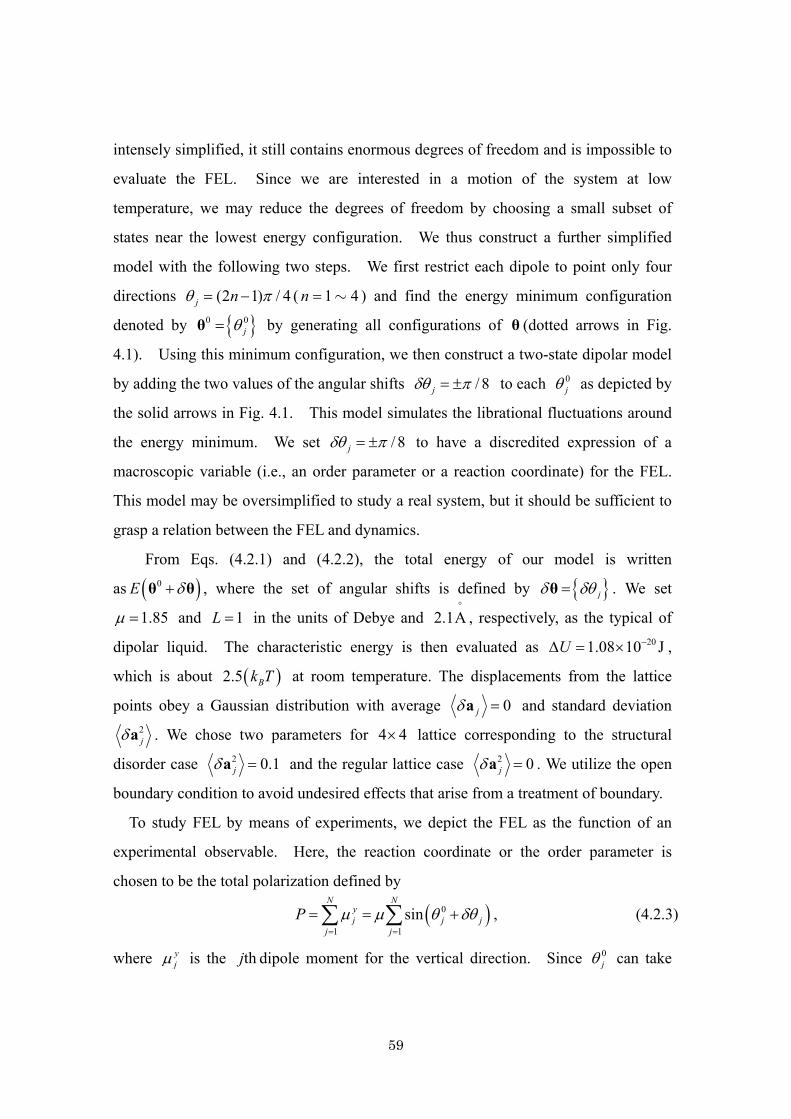
59

intensely simplified, it still contains enormous degrees of freedom and is impossible to

evaluate the FEL. Since we are interested in a motion of the system at low

temperature, we may reduce the degrees of freedom by choosing a small subset of

states near the lowest energy configuration. We thus construct a further simplified

model with the following two steps. We first restrict each dipole to point only four

directions (2 1) / 4j nθ π= − ( 1 4n = ∼ ) and find the energy minimum configuration

denoted by { }0 0jθ=θ by generating all configurations of θ (dotted arrows in Fig.

4.1). Using this minimum configuration, we then construct a two-state dipolar model

by adding the two values of the angular shifts / 8jδθ π= ± to each 0jθ as depicted by

the solid arrows in Fig. 4.1. This model simulates the librational fluctuations around

the energy minimum. We set / 8jδθ π= ± to have a discredited expression of a

macroscopic variable (i.e., an order parameter or a reaction coordinate) for the FEL.

This model may be oversimplified to study a real system, but it should be sufficient to

grasp a relation between the FEL and dynamics.

From Eqs. (4.2.1) and (4.2.2), the total energy of our model is written

as ( )0E δ+θ θ , where the set of angular shifts is defined by { }jδ δθ=θ . We set

1.85μ = and 1L = in the units of Debye and 2.1A°

, respectively, as the typical of

dipolar liquid. The characteristic energy is then evaluated as 201.08 10 JU −Δ = × ,

which is about ( )2.5 Bk T at room temperature. The displacements from the lattice

points obey a Gaussian distribution with average 0jδ =a and standard deviation 2jδa . We chose two parameters for 4 4× lattice corresponding to the structural

disorder case 2 0.1jδ =a and the regular lattice case 2 0jδ =a . We utilize the open

boundary condition to avoid undesired effects that arise from a treatment of boundary.

To study FEL by means of experiments, we depict the FEL as the function of an

experimental observable. Here, the reaction coordinate or the order parameter is

chosen to be the total polarization defined by

( )0

1 1sin

N Nyj j j

j jP μ μ θ δθ

= =

= = +∑ ∑ , (4.2.3)

where yjμ is the thj dipole moment for the vertical direction. Since 0

jθ can take

60

only (2 1) / 4j nθ π= − and we chose / 8jδθ π= ± , P takes discrete 1N + values for

N dipolar system with the constant step size ( )2 sin / 8P μ πΔ = . If N+ ( )N− is

the number of dipoles whose 0jθ satisfies 00 jθ π≤ < ( )0 2jπ θ π≤ < , the minimum

and maximum values of the reaction coordinate become

( ) ( )( )min sin / 8 sin 3 / 8P N Nμ π π+ −= − and ( ) ( )( )max sin 3 / 8 sin / 8P N Nμ π π+ −= − ,

respectively. For our model, N+ and N− satisfy / 2N N N+ −= = because the

systems are symmetric with the exclusion of the small deviated positions of dipoles.

The values of P is expressed by introducing an integer k which meets

/ 2 / 2N k N− ≤ ≤ in a symmetric form as

( ) 2 sin8

P k k πμ ⎛ ⎞= ⎜ ⎟⎝ ⎠

. (4.2.4)

The FEL is then given by

( )2

( ),1

( ) ln expN

i

iB P k P

i B

EF P k k T

k Tδ

=

⎛ ⎞= − −⎜ ⎟

⎝ ⎠∑ (4.2.5)

where iP and iE are the polarization and energy for the i th state, respectively, and

,a bδ is the Kronecker’s delta. We denote the polarization for the i th state by iP

and the reaction coordinate specified by an integer k by ( )P k .

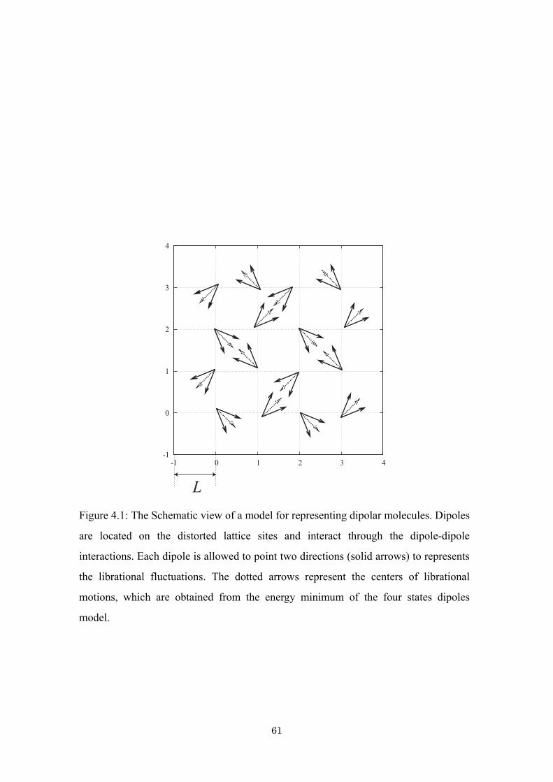
61

-1

0

1

2

3

4

-1 0 1 2 3 4

L

Figure 4.1: The Schematic view of a model for representing dipolar molecules. Dipoles

are located on the distorted lattice sites and interact through the dipole-dipole

interactions. Each dipole is allowed to point two directions (solid arrows) to represents

the librational fluctuations. The dotted arrows represent the centers of librational

motions, which are obtained from the energy minimum of the four states dipoles

model.

62

4.3 Dynamics and Observable of Dipolar System A. Master Equations for Single and Single-Double Flips Dynamics

First we should point out that our system is not kinetic, since our Hamiltonian is

specified by the configurations of the discretized dipoles and does not have a kinetic

term. To yield the time-evolution, we assume a stochastic dynamics among the

dipole states that brings the system to be in the thermal equilibrium state at t →∞ .

We do not use kinetic Monte Carlo (MC) approach introduced by Glauber [43], since

we must study dynamics at very low temperature, where the MC sampling does not

work properly. Taking an advantage of a small system, we use the master equation

approach for all 2N dipolar states. Since the master equation employs a probability

distribution function and does not rely on the sampling procedure, we can numerically

calculate the time-evolution of the system at the same CPU at any temperatures. We

ordered 2N states as 1 2 2NE E E< < < , where kE is the interaction energy

evaluated from Eq.(4.2.1) for the kth lowest energy state 0kθ θδ+ . The polarization of

kδθ is evaluated from Eq.(4.2.3) and is expressed as kP . We denote the probability

distribution for all states by vector ( ) 1 2 2( ), ( ), ( )N

tt t t tρ ρ ρ ρ⎡ ⎤= ⎣ ⎦ . This master

equation is a rate equation for the probability distributions and is expressed as

( ) ( )t ttρ ρ∂

= −∂

L , (4.3.1)

where −L is the transition matrix whose element ( )kl−L describes the transition

probability between the lth and kth states. We introduce the polarization vector given

by ( )( ) P kk

P P k D= ∑ , where

1 2 3 2

( ) ( ), ( ), ( ), ( ),, , , ,N

t

P k P k P P k P P k P P k PD δ δ δ δ⎡ ⎤= ⎣ ⎦ . (4.3.2)

The operator ( )P kD allows us to calculate the probability to have the polarization

( )P k from the probability distribution function ( )tρ . The total polarization is then

expressed as

( ) ( )P t P tρ= ⋅ , (4.3.3)

63

where the dot represents the inner product.

As was mentioned in Chapter 1, the FEL may be the same for the same system

with different dynamics. To illustrate this point, we consider two cases of −L that

can be specified by the connectivity coefficient of dipolar states. Consider the qth

lowest energy state qδθ . Suppose if we flip a dipole and energy becomes pE , the

connectivity coefficients are specified as ( )1, 1p qC = . Letting be unreachable p ′ th states

from qth state with a single dipole flipping, the coefficients satisfy ( )1, 0p qC ′ = for the

single flip case. If the state is in the qth lowest energy state qδθ and if the energy

becomes pE with a two-dipolar flipping, we set ( )2, 1p qC = and ( )2

', 0p qC = for

unreachable p ′ th state for the double flip case. The connectivity coefficients for n

flipping of dipoles ( ),n

p qC can also be defined accordingly. In Monte Carlo approach,

n=1 corresponds the single flip sampling per one MC step yielding the Glauber

dynamics, whereas n=2 corresponds to the double flip sampling. Since −L has to

satisfy the detailed balance condition, transition matrixes for n flipping dynamics have

to be in the form of

( ) ( )

( )

, ,( ),

,

exp / for ( )

for

ni j i j B i jn

i j ni j i j

C E k T E E

C E E

⎧ −Δ >⎪− = ⎨<⎪⎩

L , (4.3.4)

where ,i jEΔ is the energy difference between i th and j th states, i.e.

,i j i jE E EΔ = − . Here, we consider the linear combination of n=1 and 2 flippings

defined by

(1) (2)L L Lα β− = − − (4.3.5)

to discuss the different dynamics by a choice of the constants α andβ .

B. Laser-System Interactions To calculate response functions, we need to implement an external perturbation

based on physical considerations, since our model is not kinetic system. When we

apply an external field B to the system, the total energy of the system increases as

jP B− for the j th state. If B is small enough, we can expand the transition matrix

64

for the total Hamiltonian in terms of B. For the single flip case n=1, this is written as

( ) ( )( ) ( )1t B ttρ ρ∂

= − +∂

L μ , (4.3.6)

where −μ is the dipolar interaction whose elements are given by

( )1

, ,,

( ) / for 0 for

i j i j Bi j

P k T i ji j

⎧ − Δ >⎪= ⎨<⎪⎩

Lμ (4.3.7)

with ,i j i jP P PΔ = − . As discussed for −L , we may define the excitation for any

flipping number n. As we need to excite the system in the same manner to study the

effects of different time-evolution, we consider the single flip excitation case only.

C. First- and Third-Order Response Functions The optical observable of the system is expressed as the response functions of

dipole moment or polarization.[81] For the first-order linear and third-order

two-dimensional (2D) infrared, far infrared and THz spectroscopies, the signals are

expressed in terms of a dipole operator μ̂ as ( ){ }1 1ˆ ˆˆ ˆ( ) ( ) /eqS t i tr G tμ μ ρ×= and

( ){ }3 33 1 3 1

ˆ ˆ ˆˆ ˆ ˆ ˆ( ,0, ) ( ) ( ) /eqS t t i tr G t G tμ μ μ μ ρ× × ×⎡ ⎤= ⎣ ⎦ [86], where ˆeqρ is the equilibrium

distribution and we define ˆ ˆˆ ˆ/ [ , ] /iA B i A B× ≡ in the quantal case or ˆ ˆˆ ˆ/ { , }iA B A B× ≡ in the classical case.[122] By using the quantal or classical Liouville

operator of the system L̂ , the time-evolution operator is expressed as ˆ ˆ ˆ( ) e LtG t A A−≡ .

For the master equation, the response functions are expressed as

( ) ( )1 1( ) ( ),k

S t P k H P k t=∑ μ , (4.3.8)

and

( )3 1 3 1( ,0, ) ( ) ( ), , 0,k

S t t P k H P k t t=∑ μμμ , (4.3.9)

where

( )( ) ( ) [ ]1 1, exp eqP kH P k t D t ρ= −μ L μ , (4.3.10)

and

65

( )( ) ( ) [ ] [ ]3 1 3 1, ,0, exp exp eqP kH P k t t D t t ρ= ⋅ − −μμμ L μμ L μ . (4.3.11)

The vector eqρ represents the thermal equilibrium distribution whose component is

defined by

( ) ( )exp / /eq i BiE k T Zρ = − , (4.3.12)

in which Z is the partition function. Analogues to a quantal case, the right-hand

side of Eqs.(4.3.10) and (4.3.11) can be read from the right to left as follows. The total

system is initially in the equilibrium state eqρ . The initial state is then modified by the

first laser pulses via the dipole operator as μ at 0t = and is propagated for time 1t

by [ ]1exp t−L . The probability distribution functions is now given by [ ]1exp eqt ρ−L μ .

The linear absorption (1D) signal is the expectation value of polarization given by

( )1( ) ( ),kP k H P k t∑ μ . In the third-order 2D measurements, after the first excitation

and time evolution for 1t , the system is further excited by the second and third dipole

interactions expressed as μμ . After these excitations, the system is propagated for the

time period 3t by [ ]3exp t−L as [ ] [ ]3 1exp exp eqt t ρ− −L μμ L μ and, finally, the

expectation value of the dipole moment at 1 3t t+ is obtained by

( )3 1( ) ( ), , 0,kP k H P k t t∑ μμμ . Using the above procedure, we can calculate 1D and 2D

signals from master equation approach.

4.4 Free Energy Landscapes In Fig. 4.2, we illustrate the free energy landscapes (FELs) in the case of 4 4×

distorted and regular lattice at various temperatures: (a) 10T = , 2 0.1jδ =a ; (b)

1T = , 2 0.1jδ =a ; (c) 0.1T = 2 0.1jδ =a ; (d) 10T = , 2 0jδ =a ; (e) 1T = , 2 0jδ =a ; and (f) 0.1T = , 2 0jδ =a . Here and after, we set 1Bk = . We analyze the

temperature dependence of the heat capacity and find a sharp peak 1cT ≈ that are

corresponded to the freezing temperature of dipolar librational motions. Therefore the

cases for (c) and (f) are in the glassy state. These landscapes are directly calculated

66

from Eq. (4.2.5) by generating all possible dipolar states numerically.

To elucidate a profile for each of FELs, we introduce the density of states as the

function of ( )P k , and E expressed as

( )( ) ( )( ) ( )( ), ,n P k E dE P k g P k E dE= Ω (4.4.1)

where ( )( ),g P k E is the distribution of the density of state between E and E dE+

for fixed ( )P k and ( )( )P kΩ is the total number of states for ( )P k defined by

( )( ) ( ) ( )/ 2

/ 2 / 2!

/ 2 ! / 2 !

N

N r N r kr k

NP k C CN k N k−

=

Ω = =+ −∑ . (4.4.2)

From Eq. (4.4.1), the FEL given by Eq. (4.2.5) is evaluated as

( )( ) ( )( ) ( ) ( )( )*ln , exp /B BF P k k T dEg P k E E k T TS P k= − − −∫ , (4.4.3)

where ( )( ) ( )( )* lnBS P k k P k= Ω is the configuration entropy given by

( )( )* 1 1 1 1ln ln2 2 2 2B

k k k kS P k k N

N N N N⎡ ⎤⎛ ⎞ ⎛ ⎞ ⎛ ⎞ ⎛ ⎞

− + + + − −⎢ ⎥⎜ ⎟ ⎜ ⎟ ⎜ ⎟ ⎜ ⎟⎢ ⎥⎝ ⎠ ⎝ ⎠ ⎝ ⎠ ⎝ ⎠⎣ ⎦

. (4.4.4)

If we assume the energy distribution ( )( ),g P k E obeys Gaussian form with the

central energy ( )( )E P k and the standard deviation ( )( )E P kΔ , Eq. (4.4.3) is

evaluated as

( )( ) ( )( ) ( )( ) ( )( )2

*

2 B

E P kF P k E P k TS P k

k TΔ

= − − . (4.4.5)

The profile of the FEL is governed by the configuration entropy ( )( )*S P k at high

temperature. By expanding ( )( ) ( )( )*F P k TS P k≈ − in power of ( )P k up to

the fourth order, we have

( ) 2 4

2 4

2 4ln 23B

F P P Pk TN P N P N

⎡ ⎤⎛ ⎞ ⎛ ⎞≈ − − −⎢ ⎥⎜ ⎟ ⎜ ⎟Δ Δ⎝ ⎠ ⎝ ⎠⎢ ⎥⎣ ⎦ (4.4.6)

where ( )2 sin / 8P μ πΔ = . Analogues to the electron transfer case [26], this result

indicates that the profile of the FELs is parabolic for the small P, while an additional

quartic contribution to the FELs is found for the large P. Since the quartic term arises

67

from ( )( )*TS P k , this contribution is attributed to the entorpic origin. In the case of

Figs. 4.2(a) and 4.2(d), the FEL is looks parabolic in the small region of P.

When the temperature drops, the simulated FELs are no longer smooth and a

remarkable difference appears between the distorted case (Fig. 4.2(c)) and the regular

case (Fig. 4.2(f)). This feature can be explained from the distribution of states as a

function of the polarization P and the energy E as illustrated in Fig. 4.3. For the

regular case, the states are highly degenerated (the close circles in Fig. 4.3) due to the

symmetry of the system, while for the distorted case, the states are not degenerated and

irregularly distributed (the open circles in Fig. 4.3) because of the frustrated

interactions among the dipoles. Since the FELs are determined by the lowest energy

states at very low temperature due the Boltzmann factor in Eq. (4.2.5), the FEL of the

distorted lattice exhibits prominent irregular profiles.

68

-13-12-11-10

-9-8-7-6-5

-7.6-7.4-7.2

-7-6.8-6.6-6.4-6.2

-6

-7.6-7.4-7.2

-7-6.8-6.6-6.4-6.2

-6

-0.6 -0.4 -0.2 0 0.2 0.4 0.6

-13-12-11-10

-9-8-7-6-5

-7.4

-7.2

-7

-6.8

-6.6

-6.4

-6.2

-7.2

-7

-6.8

-6.6

-6.4

-6.2

-0.6 -0.4 -0.2 0 0.2 0.4 0.6

(a)

(b)

(c)

(d)

(e)

(f)

T =10 T =10

T =1 T =1

T = 0 1. T = 0 1.

P N/ P N/

Distorted lattice Regular latticeF

PN

()/

FP

N(

)/F

PN

()/

Figure 4.2: The FELs as the function of the polarization P in the case of 4 4×

distorted and regular lattices at various temperatures: (a) 10T = , 2 0.1jδ =a ; (b)

1T = , 2 0.1jδ =a ; (c) 0.1T = 2 0.1jδ =a ; (d) 10T = , 2 0jδ =a ; (e) 1T = , 2 0jδ =a ; and (f) 0.1T = , 2 0jδ =a .

69

P P

E EΔP ΔP

(a) (b)

Figure 4.3: The schematic pictures of the distribution of states as a function of the

polarization P and energy E . The solid line represents FELs for (a) a regular lattice

case and (b) a distorted lattice case. The states are highly degenerated due to the

symmetry of the system shown as the close circle, while the states are degenerated and

irregularly distributed shown as the open circle in (b). As a result, the FEL for the

distorted case exhibits prominent irregular profiles.

70

4.5 Optical Responses A. One-Dimensional Signals

Following the procedures explained in Sec. 4.3.C, we have calculated the first-

and third-order response functions and plotted them as the signals in one- and

two-dimensional spectroscopies. In Figs. 4.4 (a)-(f) , the linear absorption (1D)

signal ( )1S t for (i) the single-flip case, 1α = and 0β = (solid line), and (ii) the

single-double mixed flips case, 0.5α = and 1β = (dashed line), are plotted for the

same sets of parameters 2jδa and T used in Figs. 4.2 (a)-(f). Although the

relaxation rates are different in each case, we find that solid and dashed lines in Figs.

4.4(a) and 4.4(d) at the high temperature case are well fitted by a single exponential

function, whereas the solid and dashed lines in Figs. 4.4(b) and 4.4(e) are fitted by the

sum of exponential functions at the intermediate temperature. At the low temperature,

the solid lines are single exponential function, while the dashed lines are represented

by the sum of exponential functions in Figs. 4.4(c) and 4.4(f).

To investigate these features, we consider a relaxation mode analysis, which

utilizes the eigenvalues and eigenmodes of the master equation for a system with

complex interactions.[123][124] In this analysis, the time-relaxation of a two-body

correlation function is characterized by a sum of exponential functions with their decay

rates defined by the eigenvalues of the master equation. If the number of the

eigenmodes involved in the system is enormous and the eigenvalues are well

distributed in the energy space due to the complex interactions in the system, the signal

decays non-exponentially as shown in the case of a two-dimensional ± Ising model at

the critical point. Despite the complexity of the interactions between the dipoles,

present results decay more or less exponentially regardless of the temperatures. This is

because the excitation induced by laser pulses is highly symmetrical against to P and

therefore the laser interaction excites only a few modes which decay exponentially.

To see this point more closely, we depict ( )1,H P tμ given in Eq.(4.3.10) which

represents the deviation of the distribution from the equilibrium state after the laser

interaction μ at time 0t = for given P . Figures 4.5 (a)-(f) illustrate the change of

71

( )1,H P tμ in time for distorted cases and regular lattice cases at different temperatures

for the single flip dynamics in the same order of Figs. 4.4 (a)-(f). In each figure, the

line above the P axis shows the corresponding FEL. Here, we plot the single flip

case only, since the profiles of ( )1,H P tμ for different temperatures and

configurations in the single flip and single-double flips cases are approximately

analogues, if we normalized the time scale of each figures by their relaxation rates

estimated from Fig. 4.4. As all figures in Fig. 4.5 indicate, the primary cause of the

signal relaxation is not from the movement of ( )1,H P tμ toward the 0P = point but

from the decrease of ( )1,H P tμ for the fixed position of P. Since ( )1,H P tμ decays

monotonically with keeping their profiles at the high temperature and very low

temperature as shown in Figs. 4.5 (a) and (d) and Figs. (c) and (f), respectively, we

may conclude that the excited states are composed of either the single eigenmode or

the eigenmodes that have similar eigenvalues. At the intermediate temperature in Figs.

4.5(b) and 4.5(e), the profile of ( )1,H P tμ slightly change as time goes indicating

those excite states are composed of the eigenmodes with different eigenvalues.

72

0

0.2

0.4

0.6

0.8

1

0

0.2

0.4

0.6

0.8

1

0

0.2

0.4

0.6

0.8

1

0 1 2 3 4 5

0

0.2

0.4

0.6

0.8

1

0

0.2

0.4

0.6

0.8

1

0

0.2

0.4

0.6

0.8

1

0 1 2 3 4 5

Distorted lattice Regular lattice(a)

(b)

(c)

(d)

(e)

(f)

T =10 T =10

T =1 T =1

T = 0 1. T = 0 1.

α β=1 0. , =0.0

α β=1 0. , =0.0

α β=1 0. , =0.0

α β=1 0. , =0.0

α β=1 0. , =0.0

α β=1 0. , =0.0

α β= 0 5. , =1.0

α β= 0 5. , =1.0

α β= 0 5. , =1.0

α β= 0 5. , =1.0

α β= 0 5. , =1.0

α β= 0 5. , =1.0

t1 t1

St 1(

)S

t 1()

St 1(

)

Figure 4.4: The linear absorption (1D) signals ( )1S t for (i) single flip case, 1α =

and 0β = (solid line), and (ii) single-double mixed flips case, 0.5α = and 1β =

(dashed line), are plotted for the same sets of parameters 2jδa and T used in Fig.

4.2. The intensities of the signals are normalized by their initial values.

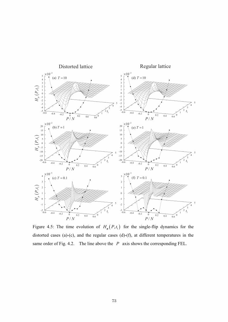
73

× −10 5 × −10 3

× −10 2

× −10 2 × −10 2

t1

t1

t1

t1

t1

t1

(a)

(b)

(c)

(d)

(e)

(f)

Distorted lattice Regular lattice

T = 0 1. T = 0 1.

T =1 T =1

T =10 T =10

HP

tμ

, 1(

)H

Pt

μ, 1

()

HP

tμ

, 1(

)

P N/

P N/

P N/

P N/

P N/

P N/

0 1

2 3

4 5

-0.6 -0.4 -0.2 0 0.2 0.4 0.6

-5-4-3-2-1 0 1 2 3 4 5

0 1

2 3

4 5

-0.6 -0.4 -0.2 0 0.2 0.4 0.6

-20

-15

-10

-5

0

5

10

15

20

0 1

2 3

4 5

-0.6 -0.4 -0.2 0 0.2 0.4 0.6

-2

-1

0

1

2

3

4

0 1

2 3

4 5

-0.6 -0.4 -0.2 0 0.2 0.4 0.6

-5-4-3-2-1 0 1 2 3 4 5

0 1

2 3

4 5

-0.6 -0.4 -0.2 0 0.2 0.4 0.6

-20

-15

-10

-5

0

5

10

15

20

0 1

2 3

4 5

-0.6 -0.4 -0.2 0 0.2 0.4 0.6

-3

-2

-1

0

1

2

3

× −10 2

Figure 4.5: The time evolution of ( )1,H P tμ for the single-flip dynamics for the

distorted cases (a)-(c), and the regular cases (d)-(f), at different temperatures in the

same order of Fig. 4.2. The line above the P axis shows the corresponding FEL.

74

B. Two-Dimensional Signals While we couldn’t observe any features specific to the FELs from 1D

measurements, we have investigated their third order response function ( )3 1,0,S t t .

We plot contour maps of 2D signals defined by ( )3 1,0,S t t for the distorted and

regular lattice cases at different temperatures in the same order as in Fig. 4.2. Figure

4.6 is for single-flip ( 1, 0α β= = ), while Fig. 4.7 is for single-double mixed flips

( 0.5, 1.0α β= = ) dynamics. Compared with the 1D case, 2D spectroscopy is much

more sensitive to the difference of temperatures, configurations of dipoles, and

dynamics. As can be seen in Figs. 4.2(a) and 4.2(d), the FELs at the high temperature

are similar due to the entropic contributions. The corresponding 2D signals in Figs. 4.6

(a) and 4.6(d) or Figs. 4.7(a) and 4.7(d) show a similar 2D profile, if we normalize the

time scales by the relaxation times estimated from Fig. 4.4. First we should notice that

if the dipole element of the laser interaction is a linear function of the system

polarization P, the 2D signals will be vanished for a harmonic potential due to the

destructive interference of the multiple laser excitations.[86] Although there is always

a quartic anharmonicity in the FELs as illustrated in Eq. (4.4.6), its contribution is too

small to have the signals comparable to the calculated results. In the present case, it is

the nonlinearity that causes 2D signals for the high temperature parabolic potential.

Based upon the profile analysis between the initial equilibrium distribution and the

laser excited distribution depicted in Fig. 4.5, we have found the effective dipole

element in the laser interactions is not linear but linear with the cubic function

expressed as 3P Pε− , where ε is the constant in the order of 210− . The nonlinear

contribution arises because we have constructed the dipole operator non-kinetic way

by expanding the Liouville operator with the external interaction defined with the

Boltzmann factors.

Regardless of the form of the laser interaction, the decays of signal profiles reflect

the system dynamics, since the time-evolutions of the system between the excitations

are governed by the system Liouvillian only. Thus, the 2D profiles in the high

temperature case decay monotonically as the function of 1t and 2t . For the

75

intermediate and lower temperature cases as shown in Figs. 4.2(b), 4.2(c), 4.2(e) and

4.2(f), the anharmonicity of potential is strong and the primary cause of the signals is

the anharmonicity of the FELs rather than the nonlinearly of dipole. While the signals

for the distorted and regular cases exhibit similar profiles at high temperature as shown

in Figs. 4.6(a) and (d) and in Figs. 4.7(a) and (d), they show clear differences at low

temperature as illustrated in Figs. 4.6(c) and (f) and in Fig. 4.7(c) and (f). These signals

seem to reflect the differences of the FEL profiles presented in Fig. 4.2, indicating a

possibility to detect a profile of FEL. The sensitivity of 2D spectroscopy also suggests

a possibility to detect the difference of dynamics on the same FELs, since the profiles

depicted in Figs. 4.6 and 4.7 are different if the dynamics is different even it is

governed by the same FELs.

To see underlying dynamics on 2D signals, we plot the distribution given in Eq.

(4.3.11). Figures 4.8(a)-(f) illustrate ( )3 1, , 0,H P t tμμμ with 1 0t = in the same order

as Figs. 4.2(a)-(f) for the single flip dynamics. Although ( )3 1, , 0,H P t tμμμ is not an

observable, it is as sensitive as 2D signals for the difference of dynamics. Thus,

( )3 1, , 0,H P t tμμμ for the single-double flips case exhibits some differences from the

single flip case presented in Fig. 4.8 unlike the case of 1D spectroscopy. Since a role

of FEL can be sufficiently explained from the single flip case, here we display the

single flip case only.

For the high temperature cases shown in Figs. 4.8(a) and (d), the distribution

profiles decay monotonically reflecting the monotonic decays of signals observed in

Figs. 4.6(a) and (d). Similar behaviors are observed in Figs. 4.7(a) and (d). The

differences between Figs. 4.6(a) and (d) and 4.7(a) and (d) are their time scales which

can be adjusted by the relaxation time estimated from Fig. 4.4(a) and (d). While the

FELs of distorted and regular cases appear similar at high-temperature due to the

entropic contribution, they become different at low temperature, which reflects the

differences in the system energetics. These differences in FELs seem to be detected by

2D spectroscopy as illustrated in Figs. 4.6(b) and (e) as well as 4.7(b) and (e). The

relaxations of distributions presented in Figs. 4.8(b) and 4.8(e) are no longer

76

monotonic, because the multiple excitations involved in 2D spectroscopies excite

various modes with different relaxation constants. Since the role of relaxation depends

on the time sequence 1t and 3t , the 2D spectroscopy can provide more information

than 1D spectroscopy.

When the temperature becomes very low, a remarkable difference appears

between the distorted and regular cases. This difference can be easily explained by

comparing the time-evolution of ( )3 1, , 0,H P t tμμμ as shown in Figs. 4.8(c) and (f).

The elongation of the peak in the 3t directed in Fig. 4.6 (f) can be attributed to the

trapping of the distribution in the local minima around / 0.25P N =± as illustrated in

Fig. 4.8(f). We also have observed the trapping of ( )3 1, , 0,H P t tμμμ in the

single-double mixed flips case (not shown), but the trapped distribution decays more

quickly than the single flip case and the elongated contribution in Fig. 4.7(f) is much

smaller than that in Fig. 4.6(f). Since other 2D signals do not show the elongation, this

implies the local minimum of the FEL may be detected as the elongated peak in the 3t

direction in the 2D IR spectroscopy.

77

Figure 4.6: The contour maps of the 2D signals for the single-flip dynamics. The

intensity of each plot is normalized by its maximum or minimum value.

78

Figure 4.7: The contour maps of the 2D signals for the single-double mixed flips

dynamics ( )0.5, 1α β= = . The intensity of each plot is normalized by its maximum

or minimum value. The insets of Figs. 4.7(a) and (d) show ( )3 1,0,S t t by using the

magnified scale.

79

t3

t3

t3

t3

t3

(a)

(b)

(c)

(d)

(e)

(f)

Distorted lattice Regular lattice

T = 0 1. T = 0 1.

T =1 T =1

T =10 T =10

t3

× −10 3

P N/

P N/

P N/

P N/

P N/

P N/

0 1

2 3

4 5

-0.6 -0.4 -0.2 0 0.2 0.4 0.6

-10-8-6-4-2 0 2 4 6 8

10−

0 1

2 3

4 5

-0.6 -0.4 -0.2 0 0.2 0.4 0.6

-4

-3

-2

-1

0

1

2

3× −10 1

0 1

2 3

4 5

-0.6 -0.4 -0.2 0 0.2 0.4 0.6

-6

-4

-2

0

2

4

6× −10 9

0 1

2 3

4 5

-0.6 -0.4 -0.2 0 0.2 0.4 0.6

-10-8-6-4-2 0 2 4 6 8

10× −10 3

0 1

2 3

4 5

-0.6 -0.4 -0.2 0 0.2 0.4 0.6

-6

-4

-2

0

2

4

6× −10 1

0 1

2 3

4 5

-0.6 -0.4 -0.2 0 0.2 0.4 0.6

-4

-3

-2

-1

0

1

2

3

4× −10 7

HP

tμμ

μ,

,,

30

0(

)H

Pt

μμμ

,,

,3

00

()

HP

tμμ

μ,

,,

30

0(

)H

Pt

μμμ

,,

,3

00

()

Figure 4.8: The time evolution of ( )3 1, ,0,H P t tμμμ for the single-flip dynamics with

1 0t = for the distorted cases (a)-(c), and the regular cases (d)-(f), at different

temperatures in the same order of Figs. 4.2(a)-(f). The line above the P axis shows

the corresponding FEL.

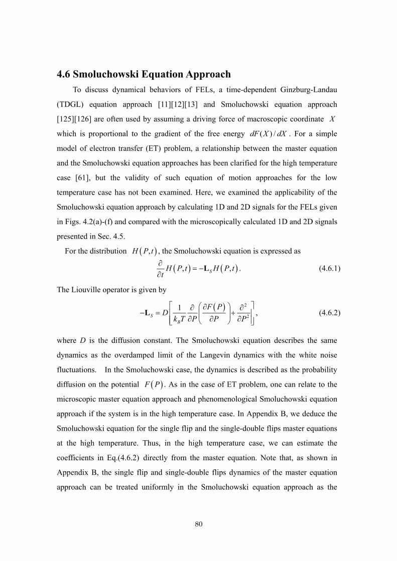
80

4.6 Smoluchowski Equation Approach To discuss dynamical behaviors of FELs, a time-dependent Ginzburg-Landau

(TDGL) equation approach [11][12][13] and Smoluchowski equation approach

[125][126] are often used by assuming a driving force of macroscopic coordinate X

which is proportional to the gradient of the free energy ( ) /dF X dX . For a simple

model of electron transfer (ET) problem, a relationship between the master equation

and the Smoluchowski equation approaches has been clarified for the high temperature

case [61], but the validity of such equation of motion approaches for the low

temperature case has not been examined. Here, we examined the applicability of the

Smoluchowski equation approach by calculating 1D and 2D signals for the FELs given

in Figs. 4.2(a)-(f) and compared with the microscopically calculated 1D and 2D signals

presented in Sec. 4.5.

For the distribution ( ),H P t , the Smoluchowski equation is expressed as

( ) ( ), ,SH P t H P tt∂

= −∂

L . (4.6.1)

The Liouville operator is given by

( ) 2

2

1S

B

F PD

k T P P P⎡ ⎤⎛ ⎞∂∂ ∂

− = +⎢ ⎥⎜ ⎟∂ ∂ ∂⎢ ⎥⎝ ⎠⎣ ⎦L , (4.6.2)

where D is the diffusion constant. The Smoluchowski equation describes the same

dynamics as the overdamped limit of the Langevin dynamics with the white noise

fluctuations. In the Smoluchowski case, the dynamics is described as the probability

diffusion on the potential ( )F P . As in the case of ET problem, one can relate to the

microscopic master equation approach and phenomenological Smoluchowski equation

approach if the system is in the high temperature case. In Appendix B, we deduce the

Smoluchowski equation for the single flip and the single-double flips master equations

at the high temperature. Thus, in the high temperature case, we can estimate the

coefficients in Eq.(4.6.2) directly from the master equation. Note that, as shown in

Appendix B, the single flip and single-double flips dynamics of the master equation

approach can be treated uniformly in the Smoluchowski equation approach as the

81

choice of diffusion parameters. Since the phenomenological features do not depend on

the diffusion parameters, here discuss the single flip case only to examine the validity

of Smoluchowski equation.

To calculate 1D and 2D signals, we need to define the dipole operator. As

mentioned in Sec. 4.5, the dipole element introduced in the master equation approach

contains the cubic polarization term. We consider the free energy with the electric

perturbation expressed as ( ) ( )3F P B P Pε− + , where B is a weak electric field and a

small constant. When we expand the free energy up to the first order by the

perturbation, we have the dipole operator in the form

26 3sB

D P Pk T P P

ε⎡ ⎤∂ ∂⎛ ⎞= − + +⎜ ⎟⎢ ⎥∂ ∂⎝ ⎠⎣ ⎦μ , (4.6.3)

where we evaluate 0.03ε=− from the master equation approach. Replacing the

Liouvillian and dipole operator in Eqs.(4.3.10) and (4.3.11) by those in Eqs.(4.6.2) and

(4.6.3), we can calculate the 1D and 2D signals from the Smoluchowski approach.

Note that the equilibrium state in the Smoluchowski approach is given by

( )( )exp /eq BF P k T∝ −ρ . In Figs. 4.9(a)-(c), we plot the 1D signals calculated from

the Smoluchowski approach for the FELs given in Figs. 4.2(a)-(f). In each figure, the

solid and dashed lines represent the distorted and regular lattice cases, respectively.

The nonlinearlity of the dipole element does not play a major role in the 1D case, since

it gives rise to a minor collection of the signals. We adjust the diffusion constants to fit

the results from the single flip master equation dynamics. For the high temperature

case, we use 7.14D = for the distorted and regular lattices which roughly agrees

with the value reduced from the master equation. In the high temperature case in

Fig.4.9(a) where the FEL profile becomes parabolic, we can analytically evaluate the

1D signals from Smoluchowski approach as described in Appendix C and the single

exponential decay of the signals, which was also observed in the master equation

approach, is explained as the relaxation of the harmonic mode. For the intermediate

and low temperature cases shown in Figs. 4.9(b) 1T = and 4.9(c) 0.1T = ,

respectively, the relaxation constants for the distorted and regular lattices are evaluated

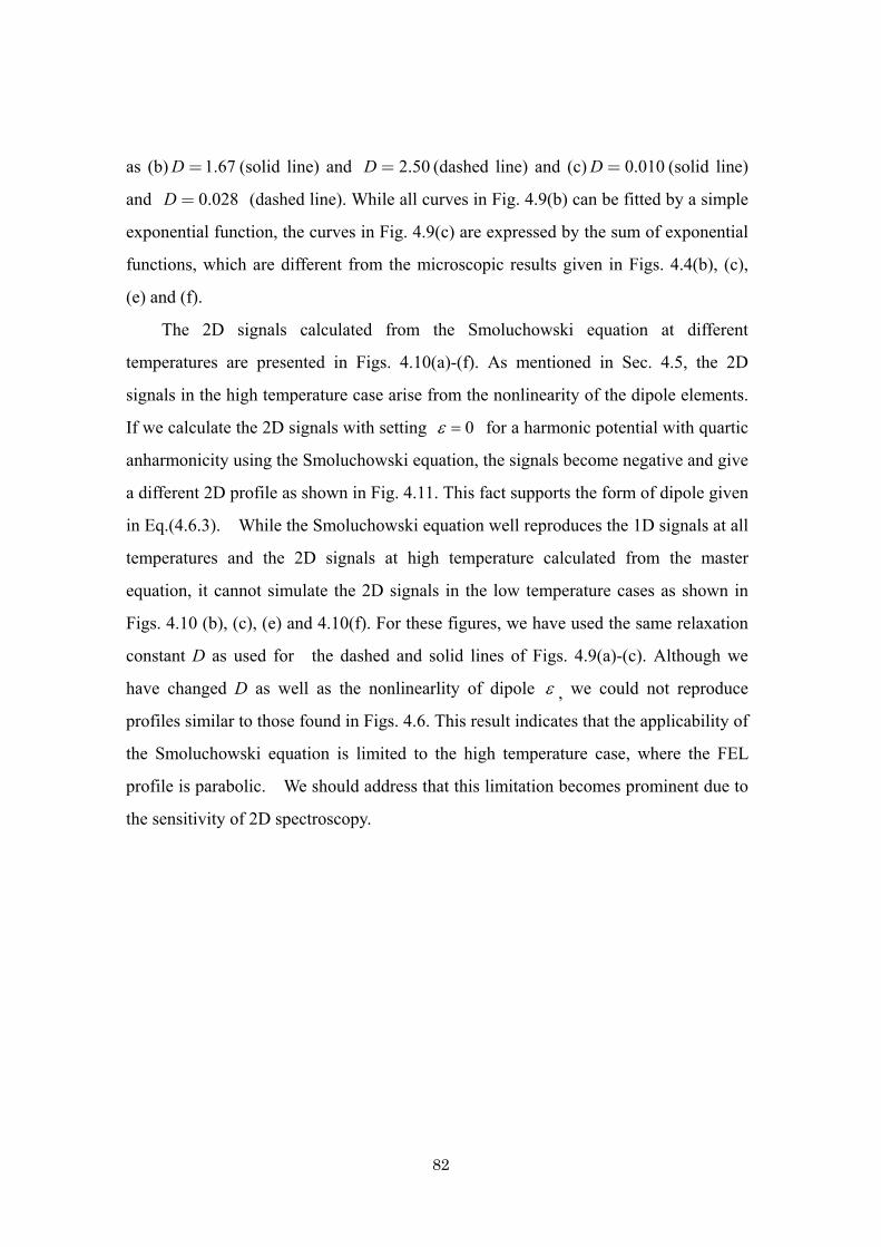
82

as (b) 1.67D = (solid line) and 2.50D = (dashed line) and (c) 0.010D = (solid line)

and 0.028D = (dashed line). While all curves in Fig. 4.9(b) can be fitted by a simple

exponential function, the curves in Fig. 4.9(c) are expressed by the sum of exponential

functions, which are different from the microscopic results given in Figs. 4.4(b), (c),

(e) and (f).

The 2D signals calculated from the Smoluchowski equation at different

temperatures are presented in Figs. 4.10(a)-(f). As mentioned in Sec. 4.5, the 2D

signals in the high temperature case arise from the nonlinearity of the dipole elements.

If we calculate the 2D signals with setting 0ε = for a harmonic potential with quartic

anharmonicity using the Smoluchowski equation, the signals become negative and give

a different 2D profile as shown in Fig. 4.11. This fact supports the form of dipole given

in Eq.(4.6.3). While the Smoluchowski equation well reproduces the 1D signals at all

temperatures and the 2D signals at high temperature calculated from the master

equation, it cannot simulate the 2D signals in the low temperature cases as shown in

Figs. 4.10 (b), (c), (e) and 4.10(f). For these figures, we have used the same relaxation

constant D as used for the dashed and solid lines of Figs. 4.9(a)-(c). Although we

have changed D as well as the nonlinearlity of dipole ε , we could not reproduce

profiles similar to those found in Figs. 4.6. This result indicates that the applicability of

the Smoluchowski equation is limited to the high temperature case, where the FEL

profile is parabolic. We should address that this limitation becomes prominent due to

the sensitivity of 2D spectroscopy.

83

(a)

(b)

t1

T =1

T = 0 1.

0

0.2

0.4

0.6

0.8

1

Distorted latticeRegular lattice

0

0.2

0.4

0.6

0.8

1

Distorted latticeRegular lattice

0

0.2

0.4

0.6

0.8

1

0 1 2 3 4 5

Distorted latticeRegular lattice

(c)

T =10

St 1(

)S

t 1()

St 1(

)

Figure 4.9: The 1D signals calculated from the Smoluchowski approach for the FELs

given in Fig. 4.2(a)-(f): (a) 10T = for the high temperature case, (b) 1T = , for the

middle temperature case and 0.1T = for the low temperature case. In each figure, the

solid and dotted lines represent the distorted and regular lattice cases, respectively.

84

Figure 4.10: The contour maps of the 2D signals calculated from the Smoluchowski

equation with the nonlinear excitation for the distorted cases (a)-(c), and the regular

lattice cases (d)-(f), at different temperatures in the same order of Figs 4.2(a)-(f). The

intensity of each plot is normalized by its maximum.

85

Figure 4.11: The contour map of the 2D signal calculated from the Smoluchowski

equation without the nonlinear excitation ( 0ε = ) for the high temperature case. The

intensity of the plot is normalized by its minimum.

86

4.7 Conclusion Having employed a simple model for the regular and the distorted dipolar systems,

we are able to have the exact FEL and collective dynamics of the system at any

temperatures, which allows us to explore a possibility to obtain information on the FEL

by spectroscopic means. The evaluated FEL exhibits the parabolic shape at high

temperature whereas it shows a bumpy profile with some minima at low temperature,

where the motion of dipoles is frozen. From the master equation approach, we

calculated the 1D and 2D singles for single flip and single-double flips dynamics.

While the 1D signals were characterized by the featureless exponential or sum of

exponential relaxation signals regardless of the FEL profiles, 2D spectra showed

distinct differences for different FEL profiles. The local minima of the FEL were

detected as the elongation of 2D signals in the 3t direction. This indicates that 2D

spectroscopy may be a useful tool to analyze FEL profile expressed as the function of

system polarization.

To examine the validity of Smoluchowski equation, we also have calculated the

1D and 2D spectra using the microscopically calculated FELs. For the high

temperature case, the dynamics described by the master equation and Smoluchowski

equation was essentially the same for the large system size thus their calculated 1D and

2D signals were the same. However, in the middle and low temperature cases, these

signals were different, which indicates that Smoluchowski equation might not be

accurate to describe the dynamics for the system with nonparabolic FELs.

Finally, we should address the limitation of the present analysis. To have the

accurate FEL with the decreasing the degrees of freedom, we had to discretize the

configuration of dipoles, which made the employment of kinetic dynamics impossible.

We thus employ the stochastic dynamics using the master equation. To make our

statement more concrete, we have to compare the present results with the kinetic ones.

For instance, although the Smoluchowski equation reproduces the stochastic results

only in the high temperature case, our statement for dynamics on the FEL may change

if we consider the kinetic system. The model dependence as well as the size

87

dependence of the present results has not been explored, which is essential to discuss a

real system.

88

89

Chapter 5 Conclusion

We have analyzed the free energy landscapes (FELs) for three types of models

representing ionic solvation, electron transfer (ET) and dipolar crystal systems in terms

of statistical and dynamical aspects. In general, the FEL is a useful concept for

explaining the static and dynamic behaviors of systems since it corresponds to the

probability of achieving a given state, and is well characterized by a simple functional

form even with complex interactions among atoms and molecules at high temperature.

One of our research interests is the structural change of the FEL depending on the

physical conditions such as temperature. For obtaining reasonable FELs, we introduced

models to decrease the degree of freedom and employed suitable calculation method,

Wang-Landau method.

The Chapter 2, a simulation model for ionic solvation in a polar solvent is

prepared, in which a central charge is surrounded by dipolar molecules posted on the

distorted lattice sites with simple rotational dynamics. The density of states is

calculated by applying the Wang-Landau algorithm to both the energy and polarization

states. The FELs of solvent molecules as the function of polarization are depicted to

explore the competition between the thermal fluctuation and solvation energy. Without

the central charge, for temperatures higher than the energy scale of the dipole-dipole

interactions, the energy landscape for the small polarization region exhibits a parabolic

shape as predicted by Marcus for ET reaction, while there is an additional quartic

contribution to the landscape for the large polarization region. When the temperature

drops, the simulated FELs are no longer smooth due to the presence of multiple local

minima arising from the frustrated interactions among the dipoles. The parabolic

contribution becomes negligible and the energy landscape becomes quartic in shape. If

the central charge is strong, the energy landscape exhibits an asymmetric profile due to

the contributions of linear and cubic terms that arise from the charge-dipole

interactions.

90

In Chapter 3, a model to simulate electron transfer (ET) reaction is prepared with

a solute dipole surrounded by dipolar molecules with simple rotational dynamics

posted on the three-dimensional distorted lattice sites. The interaction energy between

the solute and solvent dipoles as a reaction coordinate is adopted and FELs are

calculated by generating all possible states for a 26-dipolar-system and by employing

Wang-Landau sampling algorithm for a 92-dipolar-system. For temperatures higher

than the energy scale of dipole-dipole interactions, the FELs for the small reaction

coordinate region have the quadratic shape as predicted by Marcus, whereas for the

large reaction coordinate region, the shape of the landscapes is non-quadratic. When

the temperature drops, small notched structures appear on the free energy profiles

because of the frustrated interactions among the dipoles. The formation of notched

structure is analyzed with statistical approach and it is shown that the amplitude of

notched structure depend upon the segment size of the reaction coordinate and is

characterized by the interaction energy among the dipoles. Using simulated FELs, we

calculate the reaction rates as a function of the energy gap for various temperatures. At

high temperatures, the reactions rates follow a bell shaped (inverted parabolic) energy

gap law in the small energy gap regions, while the bell shape becomes steeper than the

parabolic shape in a large energy gap regions due to the FEL’s non-quadratic shape.

The peak position of the parabola also changes as the function of temperature. At low

temperatures, the profile of the reaction rates is no longer smooth because of the many

local minima of the FELs.

The other interest of our research is to explore the relationship between FEL and

system dynamics. The FEL corresponds to the thermal fluctuation of the system,

however the FEL does not perfectly govern the system dynamics. This is because the

FEL is defined by the thermal equilibrium state where the dynamical behaviors

become invisible. In addition, the FEL is a highly conceptual quantity because it is not

directly observable. Thus we introduced a model which enables us to calculate both

static and dynamic quantities and to attempt to explain the system dynamics on the

FEL by means of linear and nonlinear IR spectroscopies.

91

In Chapter 4, a model for the dipolar crystal system is employed to explore a role

of FEL, in which dipolar molecules are posted on two-dimensional lattice sites with

two-state librational dynamics. All dipole-dipole interactions are included to have

frustrated interactions among the dipoles. For the regular and distorted lattice cases, the

FEL is calculated from the interaction energies and the total polarizations for all

possible dipolar states at various temperatures. At high temperature, the shape of the

calculated FEL is smooth and parabolic, while it becomes bumpy at low temperature

exhibiting multiple local minima. To study dynamical aspects of the system, the

single flip dynamics and the single-double mixed flips dynamics of dipoles are

examined from a master equation approach. As the observables of linear absorption

and two-dimensional (2D) infrared and far infrared spectroscopies, the first- and

third-order response functions of polarization are calculated for different physical

conditions characterized by the FEL. While the linear absorption signals decay in time

in a similar manner regardless of the FEL profiles, the 2D signals exhibit prominent

differences for those profiles. This indicates that, we may differentiate the FEL profiles

by changing two-time valuables in 2D spectroscopy. As illustrated in the single-double

flips case, the FEL study by means of 2D spectroscopy, however, depends on the

dynamics which is set independently from the FEL. The Smoluchowski equation is

applied to examine the description of the collective dynamics on the microscopically

calculated FEL. We found that the 1D and 2D signals calculated from the

Smoluchowski equation agree with those from master equation only at the

temperatures where the FELs become parabolic shape.

92

93

Appendix A Brief Summary of Random Energy Model (REM)

In a framework of the random energy model (REM)[58][59], all dipole-dipole and

charge-dipole interactions are assumed to have a random Gaussian distribution

function characterized by the averaged charge-dipole and dipole-dipole interactions

)(qξ and J , and their standard deviations ξΔ and JΔ . The average solvation

energy is then given by,

( ) ( ) 2E x N x q zJxξ⎡ ⎤= +⎣ ⎦ , (A.1)

where z is the average number of dipoles interacting with each single dipoles. The

standard deviation of the solvation energy is assumed to be independent of x and

given by

2 2 2E N z Jξ⎡ ⎤Δ = Δ + Δ⎣ ⎦ . (A.2)

Introducing the probability distribution ),( Exg at polarization x as

( )( )( )2

2

1, exp22

E E xg x E

EEπ

⎡ ⎤−⎢ ⎥= −

Δ⎢ ⎥Δ ⎣ ⎦ (A.3)

yields an average density of states with polarization x and energy between E and

dEE +

( ) ( ) ( ), ,n x E Nx g x E= Ω , (A.4)

where

( )( ) ( )

! !! ! 1 / 2 ! 1 / 2 !N NNx

n n N x N x+ −

Ω = =⎡ ⎤ ⎡ ⎤− +⎣ ⎦ ⎣ ⎦

(A.5)

is the total number of states with polarization x . For 1),( >>Exn , one can

approximate ),(ln Exn by ),(ln Exn , and the entropy can be written by

( ) ( ) ( )( )( ) ( )

2

2, ln , ln ln 22

E E xS x E n x E Nx E

Eπ

−≈ = Ω − − Δ

Δ. (A.6)

94

( )( ) ( ) ( )

( ) ( )( )( ) ( )

2

REM1/ 2

12,

1 2

c

c

EE x TS Nx T T xN TF x T

E x E S Nx T T xN

∗

∗

⎧ ⎛ ⎞Δ− − >⎪ ⎜ ⎟⎪ ⎝ ⎠= ⎨

⎪ − Δ ≤⎪⎩

The above approximation is not valid below the critical energy,

( ) ( )( )1/ 22 lncE E x E Nx≈ −Δ (A.7)

since the entropy becomes negative. Therefore we set 0),( =ExS for )(xEE c< .

This result indicates a polarization-dependent phase transition at the temperature

( ) ( )cET x

S Nx∗

Δ= , (A.8)

where the configuration entropy )(* NxS is given by ( )( )NxNxS Ω= log)(* . In the

large N limit, the configuration entropy becomes

( ) 1 1 1 1ln ln2 2 2 2

x x x xS Nx N∗ ⎡ ⎤+ + − −⎛ ⎞ ⎛ ⎞ ⎛ ⎞ ⎛ ⎞= − −⎜ ⎟ ⎜ ⎟ ⎜ ⎟ ⎜ ⎟⎢ ⎥⎝ ⎠ ⎝ ⎠ ⎝ ⎠ ⎝ ⎠⎣ ⎦ (A.9)

with the aid of the Stirling’s formula. Then the free energy landscape for REM

approximation is expressed as

(A.10)

(A.11)

To determine the average number of interacting dipoles z for dipole-dipole

interactions, which affects long range, we use the following condition:

( ) ( ) ( )REM1, / 1, / 1 /F T N F T N E N= = (A.12)

Note that, in Eq. (A.12), we always use the free energy for )(xTT c≤ because )(xTc

becomes infinite when 1→x .

95

Appendix B Derivation of the Smoluchowski Equation

In this Appendix, we discuss the relation between the master equation and the

Smoluchowski equation. The time evolution of our system is given by the master

equation Eq. (4.3.1) and the probability distribution vector ( )tρ has 2N states. Here

we rewrite the Eq. (4.3.1) as the following form

( ) ( ) ( ) ( ) ( ), ,i j ii j j ij

t t ttρ ρ ρ∂ ⎡ ⎤= − − −⎣ ⎦∂ ∑ L L . (B.1)

For the high temperature case, the transition occurs absolutely if two states are

connected with given dynamics, thus the transition matrix, ( ) ( )1 2α β− = − −L L L , can

be written as

( ) ( ) ( )1 2, ,, i j i ji j

C Cα β− = +L , (B.2)

where ( ),n

i jC is the connectivity coefficient introduced in the section 4.3. Assuming a

single flip and double flips of dipole in the system whose polarization is jP , we can

construct the rate equation expressed as

( ) ( ) ( ) ( ) { }( )( ) ( ) { }( )

( ) ( ) ( ) ( ) { }( )( ) ( ) ( ) ( ) ( ) { }( )

1, , , ,

1, ,

2, , ,

2 2, , , ,

1 2

2

+ 2

i i j

j

i j

j j

i P i P j P i j i jj

j P i j i jj

i P j P i j i jj

j P i j i j j P i j i jj j

t N t t C P P Pt

t C P P P

N Nt t C P P P

t C P P t C P P P

ρ α ρ α ρ δ

α ρ δ

β ρ β ρ δ

β ρ δ β ρ δ

∂= − + − − Δ

∂

+ − + Δ

−− + − − Δ

+ − − + Δ

∑

∑

∑

∑ ∑

, (B.3)

where ( ), ii P tρ is the ith component of the probability distribution vector ( )tρ and

the subscript iP is introduced for representing the polarization of the ith state. Here

we calculate the polarization and time probability distribution function ( )( ),H P k t

by summing Eq.(B.3) over all states with the same polarization ( )P k .Operating

( ), iP k Piδ∑ to both sides of Eq.(B.3), we obtain

96

( )( ) ( )( )

( )( )

( )( )

( ) ( )( )

22

22

, ,4 2

1 ,2

1 ,2

3 1 1 3 2 ,8 4 2

N NH P k t N k H P k tt

N k H P k P t

N k H P k P t

N N k k N H P k P t

α β

α

α

β

⎡ ⎤⎛ ⎞∂= − + − +⎢ ⎥⎜ ⎟∂ ⎝ ⎠⎣ ⎦

⎛ ⎞+ + − −Δ⎜ ⎟⎝ ⎠⎛ ⎞+ + + + Δ⎜ ⎟⎝ ⎠⎧ ⎫

⎡ ⎤+ + + + − + − Δ⎨ ⎬⎣ ⎦⎩ ⎭

( ) ( )( )2

23 1 1 3 2 ,8 4 2

N N k k N H P k P tβ⎧ ⎫

⎡ ⎤+ + + + + + + Δ⎨ ⎬⎣ ⎦⎩ ⎭

. (B.4)

Here assuming ( )P k be continuous variable and taking large N limit, we get

( ) ( )2

2, ,H P t P D H P tt P P

γ⎛ ⎞∂ ∂ ∂

= +⎜ ⎟∂ ∂ ∂⎝ ⎠, (B.5)

where we set ( )2 Nγ α β= + and ( )2 / 2D N P Nα β= Δ + . The first and second

terms correspond to the drift term and diffusion terms, respectively.

97

Appendix C Linear Absorption Signal from Smoluchowski Equation Approach

If the potential is harmonic, the Smoluchowski equation for a given arbitrary

initial condition can be easily solved as

( ) ( ) 2

0, exp exp

2 2n nn

H P t a n t P H PD Dγ γγ

=

⎛ ⎞⎛ ⎞= − − ⎜ ⎟⎜ ⎟ ⎜ ⎟⎝ ⎠ ⎝ ⎠∑ , (C.1)

where ( )nH ξ are the Hermite polynomials and na are the initial values for n th

eigenfunctions. For 1D spectroscopy, the nonlinearity of dipole plays a minor role, so

we can set 0ε= in Eq.(4.6.3). At high temperature, the FEL is approximated by

parabolic function, so that the initial condition of the Smoluchowski immediately after

excitation is expressed by the first Hermite polynomial, i.e.

( ) ( ) ( )21,0 expH P H−∼ ξ ξ , where / 2DPξ γ= . Thus, the 1D signal for high

temperature is analytically evaluated as

( ) ( ) 21 1exp exp

2 2S t t dP P H P

D D

⎛ ⎞⎛ ⎞ ⎟⎜⎟⎜ ⎟− − ⎜⎟⎜ ⎟⎜⎟⎜ ⎟⎟⎝ ⎠ ⎜⎝ ⎠∫∼ γ γγ . (C.2)

This equation indicates the signal decays exponentially as the relaxation of collective

mode with the relaxation rate γ .

98

99

References

1 C. A. Angell, K. L. Ngai, G. B. McKenna, P. F. McMillan, S. W. Martin, J. Appl.

Phys. 88, 3113 (2000).

2 P. Welch and M. Muthukumar, .Phys. Rev. Lett. 87, 218302 (2001).

3 R. A. Marcus, Rev. Mod. Phys. 65, 599 (1993).

4 R. A. Marcus, J. Chem. Phys. 24, 966 (1956); 979 (1956).

5 C. L. Brooks III, M. Gruebele, J. N. Onuchic, and P. G. Wolynes , Proc. Natl. Acad.

Sci. USA, 95, 11037 (1998).

6 D. J. Wales, Energy Landscapes, (Cambridge University Press, 2004).

7 D. J. Wales and T. V. Bogdan, J. Phys. Chem. B, 110, 20765 (2006).

8 C. Chipot and A. Pohorille, Free Energy Calculations, (Springer-Verlag Berlin

Heisenberg, 2007).

9 L. D. Landau, Phys. Z. Sowjet., 11, 26 (1937); 11, 545 (1937).

10 M. Mézard, G. Parisi, and M. A. Virasoro, Spin Glass Theory and Beyond (World

Scientific, Singapore, 1987).

11 M. Cyrot, Reports on Progr. Phys. 36, 103 (1973).

12 K. Kawasaki, M. C. Yalabik, and J. D. Gunton, Phys. Rev. A, 17, 455 (1978).

13 S. Noguchi and T. Ohta, J. Phys. Soc. Jpn. 72, 1315 (2003).

14 J. R. Miller, L. T. Calcaterra, and G. L. Closs, J. Am. Chem. Soc. 106, 3047 (1984).

15 M. R. Wasielewski, M. P. Niemczyk, W. A. Svec and E. B. Pewitt, J. Am. Chem.

Soc. 107, 1080 (1985).

16 N. Mataga, T. Asahi, Y. Kanda, T. Okada and T. Kakitani, Chem. Phys. 127, 249

(1988).

17 D. F. Calef and P. G. Wolynes, J. Phys. Chem. 87, 3387 (1983).

18 D. F. Calef and P. G. Wolynes, J. Chem. Phys. 78, 470 (1983).

19 M. Tachiya, J. Phys. Chem. 93, 7050 (1989).

20 A. Yoshimori, T. Kakitani, Y. Enomoto, and N. Mataga, J. Phys. Chem. 93, 8316

(1989).

100

21 J. K. Hwang and A. Warshel, J. Am. Chem. Soc. 109, 715 (1987).

22 R. A. Kuharski, J. S. Bader, D. Chandler, M. Sprik, M. L. Klein, and R. W. Impey, J.

Chem. Phys. 89, 3248 (1988).

23 E. A. Carter and J. T. Hynes, J. Phys. Chem. 93, 2184 (1989).

24 K. Ando and S. Kato, J. Chem. Phys. 95, 5966 (1991).

25 Y. Suzuki and Y. Tanimura, J. Chem. Phys. 124, 124508 (2006).

26 Y. Suzuki and Y. Tanimura, J. Chem. Phys. 126, 054504 (2007).

27 G. Diezemann, U. Mohanty, and I. Oppenheim, Phys. Rev. E, 59, 2067 (1999).

28 T. Odagaki, T. Yoshidome, A. Koyama, and A. Yoshimori, J. Non-Cryst. Solids 352,

4843 (2006).

29 G. Adjanor, M. Athenes, and F. Calvo, Eur. Phys. J. B. 53, 47 (2006).

30 P. Welch and M. Muthukumar, .Phys. Rev. Lett. 87, 218302 (2001).

31 N. Go and H. A. Scheraga, Macromolecules, 9, 535 (1976).

32 A. Kitao, S. Hayward, and N. Go, Proteins, 33, 496 (1998).

33 A. Kitao and N. Go, Curr. Opin. Struct. Biol, 9, 164 (1999).

34 D. A. Evans and D. J. Wales, J. Chem. Phys. 119, 9947 (2003).

35 J. N. Onuchic, Z. Luthey-Schulten, and P. G. Wolynes, Ann. Rev. Phys. Chem. 48,

545 (1997).

36 J.-E. Shea, J. N. Onuchic, and C. L. Brooks, III, Proc. Natl. Acad. Scie. USA, 99,

16064, (2002).

37 P. Weinkam, C. Zong, and P. G. Wolynes Proc. Natl. Acad. Sci. USA, 102, 12401

(2005).

38 N. Go, Ann. Rev. Biophys. Bioeng. 12, 183 (1983).

39 J. N. Onuchic and P.G. Wolynes, Curr. Opin. Struct. Biol. 14, 70 (2004).

40 Y. Sugita, A. Kitao, and Y. Okamoto. J. Chem. Phys. 113, 6042 (2000).

41 M. Leitgeb, C. Schröder, and S. Boresch, J. Chem. Phys. 122, 084109 (2005).

42 W. T. Coffey, Y. P. Kalmykov, and J. J. Waldron, The Langevin Equation (World

Scientific, 2006).

101

43 R. J. Glauber, J. Math. Phys. 4, 294 (1963).

44 N. Go, J. Stat. Phys. 30, 413 (1983).

45 E. Shakhnovich, Curr. Opin. Struct. Biol. 7, 29 (1997).

46 P. F. N. Faisca and R. C. Ball, J. Chem. Phys. 116, 7231 (2002).

47 P. F. N. Faisca and R. C. Ball, J. Chem. Phys. 117, 8587 (2002).

48 R. Zwanzig, J. Chem. Phys. 38, 2766 (1963).

49 H.-X. Zhou and B. Bagchi, J. Chem. Phys. 97, 3610 (1992).

50 T.-W. Nee and R. Zwanzig, J. Chem. Phys. 52, 6353 (1970).

51 A. Papazyan and M. Maroncelli, J. Chem. Phys. 95, 9219 (1991).

52 P. G. Wolynes, J. Chem. Phys. 86, 5133 (1987).

53 L. E. Fried and S. Mukamel, J. Chem. Phys. 93, 932 (1990).

54 S. S. Komath and B. Bagchi, J. Chem. Phys. 98, 8987 (1993).

55 H.-X. Zhou, B. Bagchi, A. Papazyan, and M. Maroncelli, J. Chem. Phys. 97, 9311

(1992).

56 A. Papazyan and M. Maroncelli, J. Chem. Phys. 102, 2888 (1995).

57 J. N. Onuchic and P. G. Wolynes, J. Chem. Phys. 98, 2218 (1993).

58 B. Derrida, Phys. Rev. Lett. 45, 79 (1980).

59 B. Derrida, Phys. Rev. B. 24, 2613 (1981).

60 J. D. Bryngelson and P. G. Wolynes, J. Phys. Chem. 93, 6902 (1989).

61 V. B. P. Leite and J. N. Onuchic J. Phys. Chem. 100, 7680 (1996).

62 V. B. P. Leite, L. C. P. Alonso, M. Newton, and J. Wang, Phys. Rev. Lett. 95,

118301 (2005).

63 N. G. van Kampen, Stochastic Processes in Chemistry and Physics (North Holland

Publishing, Amsterdam, 1981).

64 Y. Tanimura, V. B. P. Leite, and J. N. Onuchic, J. Chem. Phys. 117, 2172 (2002).

65 N. Metropolis, A. Rosembluth, M. Rosembluth, and A. Teller, J. Chem. Phys. 21,

1087 (1953).

66 A. Mitsutake, A. Sugita, and Y. Okamoto, Biopolymers, 60, 96 (2001).

102

67 B. A. Berg and Neuhaus, Phys. Lett. B, 267, 249 (1991).

68 B. A. Berg and T. Newhaus, Phys. Rev. Lett. 68, 9 (1992).

69 J. Lee, J. Phys. Rev. Lett. 71, 211 (1993).

70 J. Lee, J. Phys. Rev. Lett. 71, 2353 (1993).

71 F. Wang and D. P. Landau, Phys. Rev. Lett. 86, 2050 (2001).

72 F. Wang and D. P. Landau, Phys. Rev. E 64, 056101 (2001).

73 M. Mezei, J. Comput. Phys. 68, 237 (1987).

74 C. Bartels and M. Karplus, J. Phys. Chem. B, 102, 865 (1998).

75 B. A. Berg and T. Celik, Phys. Rev. Lett. 69, 2292 (1992).

76 U. H. E. Hansmann, and Y. Okamoto, J. Comput. Chem. 14, 1333 (1993).

77 N. Urakami and M. Takasu, J. Phys. Soc.. Jpn. 65, 2694 (1996).

78 H. Noguchi and K. Yoshikawa, J. Chem. Phys. 109, 5070 (1998).

79 H. Okumura and Y. Okamoto, Chem Phys. Lett. 391, 248 (2004).

80 H. Okumura and Y. Okamoto, Phys. Rev. E 70, 026702 (2004).

81 S. Mukamel, Pronciples of Nonlinear Optical Spectroscopy, (ford University Press,

New York, 1995).

82 Y. Tanimura and S. Mukamel, J. Chem. Phys. 99, 9496 (1993).

83 K. Okumura and Y. Tanimura, J. Chem. Phys. 106, 1687 (1997).

84 K. Okumura and Y. Tanimura, J. Chem. Phys. 107, 2267 (1997).

85 Y. Tanimura, Chem. Phys. 233, 217 (1998).

86 Y. Tanimura, J. Phys. Soc. Jpn. 75, 082001 (2006).

87 P. Hamm, M. Lim, and R. M. Hochstrasser, Phys. Rev. Lett. 81, 5326 (1998).

88 P. Hamm, M. Lim, and R. M. Hochstrasser, J. Phys. Chem. B 102, 6123 (1998).

89 L.J. Kaufman, J. Heo, L.D. Ziegler, and G.R. Fleming, Phys. Rev. Lett. 88, 207402

2002).

90 K.J. Kubarych, C.L. Milne, S. Lin, V. Astinov, and R.J.D. Miller, J. Chem. Phys.

116, 2016 (2002).

91 A. Ma and R. M. Stratt, Phys. Rev. Lett. 85, 1004 (2000).

103

92 T. L. C. Jansen, J. G. Snijders, and K. Duppen, J.Chem. Phys. 114, 10910 (2001).

93 S. Saito and I. Ohmine, Phys. Rev. Lett. 88, 207401 (2002).

94 J. Cao, S. Yang, and J. Wu, J. Chem. Phys. 116, 3760 (2002).

95 Y. Nagata and Y. Tanimura, J. Chem. Phys. 124, 024508 (2006).

96 R. R. Ernst, G. Bodenhausen, and A. Wokaun, Principles of Nuclear Magnetic

Resonances in One and Two Dimensions (Clarendon, London, 1987).

97 K. Okumura, A. Tokmakoff, and Y. Tanimura, Chem. Phys. Lett. 314, 488 (1999).

98 K. Okumura, D. M. Jonas, and Y. Tanimura, Chem. Phys. 266, 237 (2001)

99 S. Hahn, K. Kwak, and M. Cho, J. Chem. Phys. 112, 4553 (2000).

100 Y. Nagata, Y. Tanimura, and S. Mukamel, J. Chem. Phys. 126, 204703 (2007).

101 N. Demirdoven, M. Khalil, and A. Tokmakoff, Phys. Rev. Lett., 89, 237401

(2002).

102 K. A. Merchant, W. G. Noid, D. E. Thompson, R. Akiyama, R. F. Loring, and M.

D. Fayer, J. Phys. Chem. B 107, 4 (2003).

103 K. F. Everitt, E. Geva, and J. L. Skinner, J. Chem. Phys. 114, 1326 (2001).

104 Y. Tanimura and K. Okumura, J. Chem. Phys, 106, 2078 (1997).

105 A. Ishizaki and Y. Tanimura, J. Chem. Phys. 125, 084501 (2006).

106 Y. Suzuki and Y. Tanimura, J. Chem. Phys. Accepted.

107 I. Benjamin, P. F. Barbara, B. J. Gertner, and J. T. Hynes, J. Phys. Chem. 99, 7557

(1995).

108 Y. Okamoto, J. Mol. Graph. Model. 22, 425 (2004).

109 B. Bagchi and A. Chandra, Adv. Chem. Phys. 80, 1 (1991).

110 B. U. Felderhof, J. Chem. Phys. 67, 493 (1977).

111 R. A. Marcus, Discuss. Faraday Soc., 29, 21 (1960).

112 A. Warshel, J. Phys. Chem. 86, 2218 (1982).

113 A. Chandra and B. Bagchi, J. Chem. Phys. 91, 7181 (1989).

114 A. Chandra and B. Bagchi, J. Chem. Phys. 94, 2258 (1991).

115 A. Milischuk and D. V. Matyushov, J. Phys. Chem. A, 106, 2146 (2002).

104

116 Y. Tanimura, H. Takano, and J. Klafter, J. Chem. Phys. 108, 1851 (1998).

117 F. H. Stillinger, Science, 267, 1935 (1995).

118 P. G. Wolynes, J. N. Onuchic, and D. Thirumalai, Science, 267, 1619 (1995).

119 P. E. Leopold, M. Montal, and J. N. Onuchic, Proc. Natl. Acad. Sci. USA, 89,

8721 (1992).

120 J. M. Luttinger and L. Tisza, Phys. Rev. 70, 954 (1946).

121 D. V. Matyushov, J. Chem. Phys. 120, 1375 (2004).

122 S. Mukamel, V. Khidekel , and V. Chernyak, Phys. Rev. E 53, R1 (1996).

123 H. Takano and S. Miyashita, J. Phys. Soc. Jpn. 64, 3688 (1995).

124 S. Koseki, H. Hirao, and H. Takano, J. Phys. Soc. Jpn. 66, 1631 (1997).

125 L. D. Zusman, Chem. Phys. 49,295 (1980).

126 H. Sumi and R. A. Marcus, J. Chem. Phys. 84, 4272 (1986).