contribution of · web viewa number of other researchers have contributed to the work found in...
TRANSCRIPT

Development of an Integrated Transport and
Emissions Model and Applications for Population
Exposure and Environmental Justice
Timothy Sider
Thesis
Department of Civil Engineering and Applied Mechanics
McGill University, Montréal
December 2013
Thesis submitted to McGill University in partial fulfillment
of the requirements for the degree of Master of Engineering
© Timothy Sider 2013


CONTRIBUTION OF AUTHORSA number of other researchers have contributed to the work found in this thesis.
The two major contributors are my co-supervisors, Professors Marianne
Hatzopoulou and Naveen Eluru, who co-authored the three research papers found
in Chapters 4-6. For development of the integrated transport and emission model,
assistance was received from: William Farrell (M.Eng candidate) for the regional
assignment model; Ahsan Alam (PhD candidate) for the running emission
simulation; and Gabriel Goulet-Langlois (B.Eng candidate) for the running and
start emission simulations. Gabriel Goulet-Langlois also contributed work to the
research on variability of emission estimates in Chapter 4. Meanwhile, Chapter 5
was co-authored by Ahsan Alam, Mohamad Zukari (B.Eng candidate), Hussam
Dugum (B.Eng candidate), and Nathan Goldstein (B.Eng candidate). Finally,
Chapter 6 was written in collaboration with Professor Kevin Manaugh.
3

ACKNOWLEDGEMENTSI would first like to acknowledge my two co-supervisors, Professors Marianne
Hatzopoulou and Naveen Eluru, for their tremendous support and guidance over
the past two and a half years. It has been a great privilege to have both as
supervisors. I would also like to thank other graduate students in the transportation
program that I’ve collaborated with, specifically William Farrell and Ahsan Alam.
At the same time, contribution to the research from a number of undergraduate
students has been invaluable. This includes Gabriel Goulet-Langlois, Mohamad
Zukari, Hussam Dugum, Nathan Goldstein, and Anthony Somos. Furthermore, I
would like to acknowledge the teachings of Professors Peter Brown, Mark
Goldberg and Nicolas Kosoy for inspiring the philosophical basis for my research
into the environmental and social impacts of our transportation systems. Finally, I
would like to thank my parents, my brother and my girlfriend, for being awesome.
Much love.
4

ABSTRACTRoad transport has a tremendous impact on local urban regions as well as global
planetary health. This impact is especially great given the large quantities of
greenhouse gases and local air pollutants released across the world, quantities that
continue to increase. For metropolitan regions, reductions in traffic-related air
pollution are paramount. Which baseline is used and which strategies should be
implemented are both vital questions in this regard. Integrated transport and
emissions models are important tools that aid metropolitan planners in answering
those questions. A regional traffic assignment model has been connected to a
detailed emission processor for the Montreal metropolitan region. The road
transport model contains details on all private driving trips across a standard 24-hr
workday, including congested link speeds and stochastic path distributions.
Meanwhile, the emissions processor incorporates local vehicle registry data and
Montreal-specific ambient conditions in the estimation of both running and start
emissions. Outputs include hourly link-level and trip-level emissions for
greenhouse gases, hydrocarbons, and nitrogen oxides. Three research studies were
then explored that were anchored by the integrated transport and emissions model.
The first involved testing model sensitivity to variations in input data and
randomness. The second study was aimed at understanding the land-use and
socioeconomic determinants of traffic-related air pollution generation and
exposure. The third study encompassed an equity analysis of social disadvantage,
traffic-related air pollution generation and exposure. Major findings include
evidence that: start emissions and accurate vehicle registry data have the biggest
impact on accurate regional emission inventories; neighbourhoods closer to
downtown tend to be low emitters while having high exposures to traffic-related
air pollution, while the opposite is true for neighbourhoods in the suburbs and
periphery of the region; and marginalized neighbourhoods with high social
disadvantage tend to have the highest exposure levels in the region, while at the
same time generating some of the lowest quantities of traffic-related air pollution.
These findings support the claim that traffic is creating environmental justice
issues at the metropolitan level.
5

RÉSUMÉ
L’impact des systèmes de transports sur les régions urbaines et la santé planétaire
est immense. Cet impact est notamment important parce-que les quantités de gaz à
effet de serre et les polluants atmosphériques continuent à augmenter autour du
monde. Pour les régions métropolitaines, les réductions de la pollution de l’air liée
à la circulation sont essentielles. Cependant, quel point de référence est appliqué,
et quelles stratégies devraient être mises en œuvre, sont deux questions vitales à
cet égard. Une simulation intégrée du transport et des émissions est un outil
important qui aide les planificateurs à répondre à ces questions. Une simulation de
la circulation régionale a été liée à un simulateur des émissions détaillées pour la
région métropolitaine de Montréal. La simulation de la circulation contient des
détails sur tous les déplacements ‘auto conducteur’ pour chaque heure d’une
journée normale de travail, incluant la vitesse de circulation encombrée, et
distributions des trajets stochastiques. Aussi, le simulateur des émissions
incorpore des données sur les types de véhicules et les conditions ambiantes
locales dans l’estimation des émissions de conduite et d’ignition. Les données
produisent sont des quantités d’émissions horaires au niveau des routes et des
déplacements pour les gaz a effet de serre, les hydrocarbures, et les oxydes
d’azote. Trois études de recherche ont été basées sur les résultats de la simulation
intégrée de la circulation et des émissions. La première examine la sensibilité de la
simulation aux variations dans les données. La deuxième évalue si l’utilisation du
sol ou les caractéristiques socio-économiques sont les déterminants de production
ou d’exposition à la pollution de l’air liée à la circulation. La troisième inclue une
analyse du désavantage social et de la production et de l’exposition à la pollution
de l’air liée à la circulation. On observe que les émissions à l’ignition et les
données d’immatriculation des véhicules ont le plus grand impact sur les
inventaires des émissions régionales. En terme d’exposition à la pollution de l’air,
les quartiers les plus proches du centre-ville ont tendance à produire le moins
d’émissions tandis qu’ils ont les niveaux d’exposition les plus élevés dans la
région, alors que l’inverse est vrai pour les quartiers de banlieue et à la périphérie.
Les quartiers caractérisés par un index de désavantage social élevé ont les niveaux
6

d’exposition les plus élevés et en même temps produisent de faibles taux
d’émissions. Ces résultats appuient l’hypothèse que la circulation contribue aux
problèmes de justice environnementale à l’échelle métropolitaine.
7

TABLE OF CONTENTS
CONTRIBUTION OF AUTHORS...................................................................................I
ACKNOWLEDGEMENTS..............................................................................................II
ABSTRACT......................................................................................................................III
LIST OF TABLES........................................................................................................VIII
LIST OF FIGURES.........................................................................................................IX
LIST OF ABBREVIATIONS...........................................................................................X
CHAPTER 1: INTRODUCTION....................................................................................1
1.1 BACKGROUND.............................................................................................................1
1.2 OBJECTIVES................................................................................................................2
1.3 THESIS STRUCTURE.....................................................................................................3
CHAPTER 2: CONTEXT................................................................................................4
2.1 INTEGRATED TRANSPORTATION AND EMISSION MODELS...........................................4
2.2 STUDY AREA..............................................................................................................7
CHAPTER 3: OVERALL MODEL STRUCTURE.....................................................11
3.1 BASE DATA SOURCES...............................................................................................13
Origin-Destination Survey.........................................................................................13
Vehicle Registry Data................................................................................................13
3.2 TRAFFIC ASSIGNMENT..............................................................................................14
3.3 VEHICLE ALLOCATION.............................................................................................15
3.4 RUNNING EMISSIONS MODEL...................................................................................16
Path Arrays................................................................................................................17
Vehicle EFs................................................................................................................17
3.5 START EMISSIONS MODEL........................................................................................18
3.6 MODEL VALIDATION................................................................................................21
Transport Model........................................................................................................21
Emissions Model........................................................................................................23
CHAPTER 4: EVALUATING THE VARIABILITY IN EMISSION
INVENTORIES................................................................................................................26
4.1 CONTEXT..................................................................................................................26
8

4.2 METHODOLOGY........................................................................................................27
4.3 RESULTS...................................................................................................................33
CHAPTER 5: LAND-USE AND SOCIOECONOMICS AS DETERMINANTS OF
TRAFFIC EMISSIONS AND INDIVIDUAL EXPOSURE TO AIR POLLUTION.42
5.1 CONTEXT..................................................................................................................42
5.2 METHODOLOGY........................................................................................................43
5.3 RESULTS...................................................................................................................46
Spatial Distribution of Emissions..............................................................................46
Statistical Analysis.....................................................................................................48
5.4 CONCLUSIONS...........................................................................................................53
CHAPTER 6: EQUITY IN THE GENERATION AND EXPOSURE TO TRAFFIC-
RELATED AIR POLLUTION.......................................................................................55
6.1 CONTEXT..................................................................................................................55
6.2 METHODOLOGY........................................................................................................58
Exposure to Traffic-Related Air Pollution.................................................................59
Social Disadvantage Index........................................................................................59
Statistical Analysis.....................................................................................................61
6.3 RESULTS...................................................................................................................62
6.4 CONCLUSIONS...........................................................................................................70
CHAPTER 7: CONCLUSIONS AND FUTURE PATHWAYS OF RESEARCH....72
REFERENCES.................................................................................................................74
9

LIST OF TABLESTable 1 – Atmospheric Conditions Used For Emission Modeling........................19
Table 2 – Comparison of Daily GHG Emission Inventories..................................24
Table 3 – Factor Analysis Results: Factor Loadings and Summarya.....................45
Table 4 – Multivariate Regression Results.............................................................49
Table 5 – Cross-Tabulation of Vehicles per Household vs. Model Year...............50
Table 6 – Comparison of Socioeconomic Variables Between SDI Deciles...........63
10

LIST OF FIGURES
Figure 1 – Population density of the MMR..............................................................8
Figure 2 – Map of the Island of Montreal and surrounding municipalities.............9
Figure 3 – Integrated modeling framework............................................................11
Figure 4 – Detailed framework..............................................................................12
Figure 5 – Road network of the MMR...................................................................15
Figure 6 – Start emissions for vehicle types and model years...............................19
Figure 7 – Start emissions for PCs as a function of soak time...............................20
Figure 8 – Comparison between measured and modelled traffic volumes............22
Figure 9 – Comparison between measured and modelled traffic volumes............22
Figure 10 – Hourly traffic volume profile on the bridges......................................23
Figure 11 – Link-level NOx emissions overlaid on a map of ambient NO2...........25
Figure 12 – Soak-time comparison........................................................................31
Figure 13 – Flowchart of changes to data inputs and model simulations..............33
Figure 14 – Sensitivity results for daily regional emission estimates....................35
Figure 15 – Daily emissions isolating for starts and season...................................38
Figure 16 – Daily emissions for travel speed aggregations and vehicle ages........39
Figure 17 – Daily emissions for different vehicle ages and types..........................39
Figure 18 – Daily start emissions for different soak-time distributions.................40
Figure 19 – Soak-time comparison of start emissions per hour.............................40
Figure 20 – Emitted NOx per person......................................................................47
Figure 21 – Link-level NOx emissions on a map of emitted NOx per person........47
Figure 22 – Exposed to NOx per km2.....................................................................48
Figure 23 – Emission factor vs. vehicle age derived from MOVES......................50
Figure 24 – Spatial distribution of the generated clusters......................................52
Figure 25 – Histogram of the raw values of the Social Disadvantage Index.........63
Figure 26 – Social Disadvantage Index deciles......................................................64
Figure 27 – Difference in rankings between SDI and exposure.............................65
Figure 28 – Sum of social disadvantage ranking and exposure ranking................66
Figure 29 – Difference in rankings between exposure and emission generation...67
Figure 30 – Ranking comparison between emission generation and exposure......68
Figure 31 – Equity of traffic-related air pollution generation and exposure..........69
11

LIST OF ABBREVIATIONSAMT – Agence Métropolitaine de Transport
CBD – Central Business District
CO – Carbon Monoxide
CO2 – Carbon Dioxide
CT – Census Tract
EF – Emission Factor
FSA – Forward Sorting Area
HC – Hydrocarbons
MMR – Montreal Metropolitan Region
MOVES – Mobile Vehicle Emissions Simulator
NO2 – Nitrogen Dioxide
NOx – Nitrogen Oxides
OD – Origin-Destination
PC – Passenger Car
PM – Particulate Matter
PPP – Polluter-Pays Principle
PT – Passenger Truck
SAAQ – Société de l’Assurance Automobile du Québec
SDI – Social Disadvantage Index
SE – Standard Error
SUV – Suburban Utility Vehicle
TAZ – Traffic Analysis Zone
TOD – Transit Oriented Development
USEPA – United States Environmental Protection Agency
VKT – Vehicle-Kilometres-Travelled
VOC – Volatile Organic Compound
12

CHAPTER 1: INTRODUCTION
1.1 Background
Transportation and its negative externalities have a significant impact on global
planetary health. As a sector, transport contributes 13.1 percent of global
greenhouse gas (GHG) emissions (IPCC, 2007) and 24 percent of Canada’s GHG
footprint (Environment Canada, 2011). Additionally, nearly half the world’s oil
usage is attributed to motorized transport, further increasing its total contribution
(Woodcock et al., 2007). Furthermore, on-road emissions are predicted to have the
highest impact on climate forcing of any economic sector in the near future (10-15
years), and the second highest impact over the long-term (100 years; Unger et al.,
2010). Road-transport, consisting of private light-duty cars and trucks, public
transit vehicles and heavy-duty freight trucks, is specifically estimated to make up
almost three-quarters of transport’s total contribution (IEA, 2012). While
technological improvements have lowered emission rates per vehicle, increases in
total vehicle-kilometres-travelled (VKT) have negated most of those gains.
At the same time, the negative externalities from road-transport have a significant
presence in urban environments. With the disappearance of urban industry over
the last few decades, road transport has now become the largest contributor of air
pollution in urban regions (Colvile et al., 2001). Local air pollutants from road
transport come in the form of carbon monoxide (CO), hydrocarbons (HC),
nitrogen oxides (NOx), and particulate matter (PM), while also contributing
significant amounts of noise pollution. Previous studies have found considerable
evidence that long-term exposure to local traffic-related air and noise pollution is
potentially dangerous to various aspects of human health including birth outcomes
(Brauer et al., 2008), children’s health (Kim et al., 2004; Zmirou et al., 2004;
Kramer et al., 2000) and respiratory and cardiovascular diseases, including lung
cancer (Gan et al., 2012; Selander et al., 2009; Chen et al., 2008; Babisch et al.,
2005; Hoek et al., 2002; and Kunzli et al., 2000).
13

Given the challenges that metropolitan regions face, road transport’s impact must
be reduced. Planners and policymakers need tools in this regard that aid in
quantifying the problem and assessing feasible solutions. Integrated transport and
emission models are the best bet in this respect. Integrated models combine two
streams of research through linkages between transportation modeling and
detailed emission modeling, a combined focus that has grown rapidly in the past
few years in light of the aforementioned issues facing metropolitan regions and the
global community at large. These integrated transport and emission models are a
crucial element for metropolitan planners in answering questions such as: What is
the carbon footprint of our metropolitan region? Who are the highest emitters?
Which neighbourhoods experience the greatest levels of traffic-related air
pollution? What steps need to be taken to reduce emissions by 15, 20, or 25%?
The purpose of this thesis is therefore to explore the various applications of an
integrated transport and emissions model with a focus on the Montreal region.
1.2 Objectives
The objectives of this thesis are as follows:
i. Development of a regional traffic assignment model for the Montreal
metropolitan region (MMR)
ii. Creation of an integrated transport and emission model that incorporates
the following details in an emission processor:
a. Vehicle allocation
b. Running emissions
c. Start emissions
iii. Evaluation of the sensitivity of emission estimates from integrated
transport and emission models to data inputs and model randomness
iv. Assessment of the extent that land-use and socioeconomic characteristics
play in determining traffic-related air pollution generation and exposure at
the zonal level in the MMR
v. Exploration of the equity of traffic-related air pollution generation,
exposure and socioeconomic status across the MMR
14

1.3 Thesis structure
The thesis begins with an overview of the context of this research. Specifically,
previous research into integrated transport and emission models is explored and a
summary of the study area (MMR) is included. From there, an entire section is
devoted to model development, which explores the creation of the regional traffic
assignment model, the emission processor, and validation of both models. The
following three chapters cover three individual research papers that were anchored
by the integrated transport and emissions model:
Chapter 4: Sensitivity of emission estimates
Chapter 5: Determinants of emissions generation and exposure
Chapter 6: Equity analysis
Each chapter has context-specific sections on literature review, methodology,
results and discussion. Finally, the thesis concludes with a summary of major
findings as well as a short overview regarding pathways of future research.
15

CHAPTER 2: CONTEXT
2.1 Integrated transportation and emission models
Research into accurately estimating emissions from road transport has been
growing over the past few decades. Unlike the estimation processes for stationary
sources such as power plants, estimating exhaust levels from mobile sources such
as road transport is quite difficult due to the numerous dimensions involved, such
as travel speeds, vehicle characteristics, ambient conditions, and more. Focussing
on private individual travel, instead of public or freight, has still resulted in a large
variety in emission models. To begin, it is important to define the term ‘emission
model’ and to describe how it interacts with transportation data inputs.
Emission modeling of mobile sources involves the use of a modeling platform to
simulate all types of emissions resulting from motor vehicles. Specifically, this
includes those occurring at engine ignition (start emissions), during vehicle
cruising (running emissions) and after engine shutdown (evaporative or soak
emissions). Running emissions have been the focus of most research given that
they typically constitute the majority of pollution emitted (Borrego et al., 2004;
Houk, 2004). A modeling platform is therefore used to generate running emission
factors (EFs) that dictate a relationship between vehicle, speed and quantity of
emitted pollutant. For instance, if a vehicle with specific characteristics (type,
model year, engine size, fuel type, presence of catalytic converter, etc.) drives at a
given speed with a certain behaviour (acceleration, deceleration, gradient) and
under particular ambient conditions (temperature, pressure, sun-exposure, etc.),
then it has an associated EF in grams per VKT. Transportation data comes into the
equation through travel speed and VKT, both considered crucial elements in
emission estimation (Smit, 2006). Overall, emission models from the previous two
decades span a wide spectrum of complexity, however this trend is neither time
dependent nor geographical in nature (ie. concentrated in developed, Western
nations). Emission models have certainly become more complex in general, yet
16

varying research objectives or data availability continue to favour the use of
simple models in many situations.
The simplest models are typically used to estimate basic national emission
inventories, for instance in Mexico (Solis and Sheinbaum, 2013), or in research
that studies the determinants of individual/household GHG footprints in regions
such as Quebec City, Canada (Barla et al., 2011), Seoul, South Korea (Ko et al.,
2011), and Oxford, England (Brand and Preston, 2010). Numerous assumptions
must be made across many of the model inputs. Transportation data is sourced
from stated VKT estimates from travel surveys, and then EFs derived from
average local fuel consumption rates are applied assuming a constant average
vehicle speed. Another set of models combine similar travel survey data with EFs
generated from an emission simulator. In North America, specifically in the Puget
Sound region of Washington (Frank et al., 2006; Frank et al., 2000), the MOBILE
series of emission modeling software developed by the United States
Environmental Protection Agency (USEPA) was used to generate more accurate
EFs for a range of pollutants and vehicle characteristics. A comparable approach
was also taken in Europe, specifically in the Sardinia region in Italy (Bellasio et
al., 2007), using the COPERT platform developed by the European Environmental
Agency (EEA). Lumbreras et al (2013) even developed a platform that created
more accurate transport and vehicle data for use in the COPERT emission
simulator in order to estimate emissions for the entire country of Spain. While
these types of models attempt to account for congestion in their composite EFs,
assumptions are still made regarding vehicle characteristics, and no sense of
spatial or temporal variation across their study areas is possible.
The spatial distribution of traffic-related air pollution on the road network is
paramount for the analysis of NOx, HCs, PM, and other local pollutants, especially
given that intra-urban variation can be larger than inter-urban variation (Crouse et
al., 2009a). Another set of models attempts to incorporate spatial issues through
the use of manual traffic counts as the transport data input. This process also
17

usually captures local variations in vehicle composition, and has been applied to
the northwest of England (Lindley et al., 1999), Beijing, China (Hao et al., 2000),
Santiago, Chile (Corvalan et al., 2002), and Beirut, Lebanon (Waked and Afif,
2012). Corvalan et al (2002) are even able to account for temporal variation by
using hourly counts.
However, the majority of research has focussed on the development of truly
integrated transport and emission models incorporating detailed road-traffic
simulations. Road-traffic networks are modeled at a macroscopic or mesoscopic
scale, and then trips are assigned to the network on an hourly basis. Output data
include VKT and average link speeds, which are both used directly in conjunction
with the EFs generated from the emissions simulator. This process has garnered
international popularity and has been employed in cities and regions such as
Hamilton, Canada (Anderson et al., 1996), Helsinki, Finland (Karppinen et al.,
2000), Antwerp, Belgium (Mensink et al., 2000), Lisbon, Portugal (Borrego et al.,
2004), Hong Kong, China (Xia and Shao, 2005), Norwich, England (Nejadkoorki
et al., 2008), and Madrid, Spain (Borge et al., 2012). Beckx et al (2009a) and Hao
et al (2010) even incorporated activity-based models into their integrated
modeling frameworks applied respectively to the Netherlands and the Greater
Toronto Area, Canada. The advantage of integrated transport and emission models
is that they are able to combine congestion-related speed effects and detailed
vehicle data, often at the individual trip level. This provides significant detail
regarding spatial and temporal variation, and allows for connections to
socioeconomics or even to dispersion models that portray how meteorological
conditions and the built environment influence pollutant concentrations (De
Ridder et al., 2008).
Meanwhile, start emissions occur at engine ignition and typically occur during the
first two to three minutes of a trip. They are considered separate from those that
are emitted during an engine’s cruising phase, and they are mostly caused by: (1)
excess gasoline due to higher fuel enrichment; and (2) poor catalytic converter
18

performance due to the large gap between engine temperature at ignition and
optimum temperature for catalytic conversion. The gap between engine and
optimum temperatures is dependent on the ambient temperature, which varies by
season, and the engine’s ignition temperature, which is related to the engine soak-
time, ie. the amount of time since the engine was turned off. Therefore, an engine
that had been turned off recently would have a smaller soak-time and thus would
have an ignition temperature that is closer to the optimum temperature of the
catalytic converter. Start emissions are especially of concern when studying HC,
CO or NOx emissions, accounting for approximately 28 percent, 31 percent and 20
percent of total on-road VOCs, CO and NOx, respectively (Houk, 2004). Previous
research that had employed the MOBILE platform implicitly account for start
emissions through the generated running EFs (Hao et al., 2010; Frank et al., 2006;
Frank et al., 2000; Anderson et al., 1996). COPERT models account for starts in a
similar fashion (Lumbreras et al., 2013; Waked and Afif, 2013; Bellasio et al.,
2007). The current generation of emission software favours a distinct separation
between running and start emissions, with start EFs used to dictate the relationship
between vehicle characteristics, soak-time and amount of pollutants emitted
during engine ignition.
This research aims to build on the advancements in integrated transport and
emission models through the development of a connected regional traffic
assignment model and a comprehensive emission processor. The regional traffic
assignment model provides accurate average link speed and VKT data, while
accurate vehicle registry data is also incorporated. An emission simulator is used
to generate both running and start EFs.
2.2 Study Area
Our study area includes the MMR, which covers an area of approximately 7,000
km2 and has a population of about 3.8 million (Statistics Canada, 2011). The
region is dominated by the island of Montreal, with approximately 47 percent of
the region’s population and 71 percent of the region’s 1.4 million employment
19

opportunities (AMT, 2010). The remainder of the region consists of two sub-
regions north of Montreal: Laval and the twenty municipalities of the North Shore,
and another two sub-regions south of the island: Longueuil and the twenty-five
South Shore municipalities. Figure 1 provides the population distribution in terms
of density across the MMR with all the major sub-regions identified. Further, the
figure identifies the central business district (CBD) in a red box.
Figure 1 – Population density of the MMR
Figure 2 highlights the major boroughs on the island of Montreal as well as the
cities of Laval to the northwest and Longueuil to the east. The CBD is located
within the Ville-Marie borough.
20

Figure 2 – Map of the Island of Montreal and surrounding municipalities
The spatial economy of the Montreal region is anchored by the CBD; 59 percent
of the region’s employment opportunities are within 10 km of downtown, while
the remaining job distribution follows a concentric distance-decay curve
(Shearmur and Coffey, 2002). The other major employment centre in the region is
found near Montreal’s main airport in Ville-Saint-Laurent/Dorval, located 10-15
km west of downtown. The imbalance between jobs and residents previously
mentioned for the island of Montreal is especially large for the CBD and
surrounding central areas. In the central areas there are 24 workers for every 10
residents, an employment surplus that is being fed by Laval, Longueuil, and other
municipalities on the North and South shores (Shearmur and Motte, 2009).
Meanwhile, the island of Montreal is connected to the other sub-regions through a
system of bridges. Five bridges connect the island to the north and five to the
south, while two bridges at either end of the island connect the peripheral eastern
and western edges. With the very high proportion of off-island and on-island
21

commuters, bridges linking the island to the rest of the region have become the
salient element of the road network. At the same time, most of the residential
growth is occurring in the periphery zones of the region particularly in the north
and south shore municipalities (AMT, 2010). Overall, there are over two million
vehicles registered in the region, resulting in a regional household vehicle
ownership rate of about 1.2 vehicles (AMT, 2010).
22
CHAPTER 3: OVERALL MODEL STRUCTURE
The integrated transport and emission model has two base data inputs (OD survey,
vehicle registry) and two inputs generated from commercial software (emission
factors, traffic data). The primary outputs include emissions at both the link- and
trip-level. Developed as part of this thesis, the emission processor is the key
element of the integrated model, incorporating all four data inputs in generating
the desired output (Figure 3). The emission processor consists of: (1) a vehicle
allocation algorithm, (2) a running emissions model, and (3) a start emissions
model. The interactions between all the elements in the integrated framework are
highlighted in detail in Figure 4. The base data sources, specifically the travel
behaviour information and the vehicle registry data, are described first. The
platform used to generate running and start EFs is the Mobile Vehicle Emissions
Simulator (MOVES) developed by the USEPA.
Figure 3 – Integrated modeling framework
23

Figure 4 – Detailed framework (emission processor outlined in red)
24

3.1 Base Data Sources
Origin-Destination Survey
The base travel data for the integrated model encompasses the 2008 origin-
destination (OD) survey conducted by the Agence Métropolitaine de Transport
(AMT), the regional transit authority in the MMR. The OD survey data contains
information on 319,915 trips conducted in the MMR; each trip is associated with a
set of attributes including origin, destination, departure time, travel mode, and
attributes of the individual performing the trip including residential location. In
addition, every trip is associated with a weight or “expansion factor” which allows
us to scale the sample up to the total population. This survey is conducted every
five years and is the primary source in Montreal for information on travel habits.
The most recent survey was conducted in 2008 and the results were released in
2010. Participants in the survey were identified through a random sample of the
Montreal population using telephone listings; the sample is validated against
census data using a wide range of variables (age, gender, employment status,
home location, work location, etc.). In 2008, 66,100 households (representing 4%
of the population) were interviewed including 156,700 individuals. Telephone
interviews took place in autumn, a time period when most urban travel habits are
stable.
Vehicle Registry Data
The vehicle registry database was obtained from the provincial registry at the
Société de l’Assurance Automobile du Québec (SAAQ) for the base year of 2011.
The SAAQ database includes vehicle ownership information for the Montreal
region at the level of the Forward Sorting Area (FSA), indicated by the first three
characters of the postal code. Within each FSA, the total number of vehicles by
type (e.g. passenger car (PC), sports utility vehicle, minivan, small truck, large
truck) and model year (1981-2011) is provided. The SAAQ data contains 12
vehicle designations. These designations were collapsed into two groups, one for
PCs and one for passenger trucks (PTs; which includes SUVs, minivans, and pick-
up trucks).
25

While it is possible that the 12 vehicle designations have different emission
profiles, it is important to recognize that vehicle emissions on roadways are not
only dependent on vehicle types and models but also influenced by fuel and
engine technology, engine displacement, model year group, and regulatory class
(USEPA, 2010). In fact the emission differences between different PCs of the
same model year (and regulatory class) undergoing the same drive-cycle are
smaller than emission differences for the same car undergoing different driving
patterns. In real-road conditions, the differences due to vehicle make within the
same category (PT or PC) can be neglected. For this reason the USEPA’s model
MOVES 2010 has aggregated passenger vehicles into two broad categories: (1)
PCs (i.e. all sedans, coupes, and station wagons manufactured primarily for the
purpose of carrying passengers) and (2) PTs (which includes SUVs, minivans, and
pick-up trucks) coming from a larger vehicle classification which was included in
the older MOBILE6 series. The distribution of the fleet was computed for each
FSA, based on the two vehicle types and thirty model years provided.
3.2 Traffic Assignment
A regional traffic assignment model was developed for the MMR (Figure 5). The
model takes as input the 2008 OD trip data for the MMR provided by the AMT
and assigns it on the road network using a stochastic assignment in the VISUM
platform (PTV Vision, 2009). The regional network consists of 127,217 road links
and 90,467 nodes associated with 1,552 traffic analysis zones (TAZs). All levels
of road types were included in the model, ranging from expressways to arterials to
local roads. It also contains various road characteristics such as length, speed
limit, capacity, and number of lanes, as well as intersection characteristics such as
capacity and turning restrictions.
Only the driving trips were extracted from the OD survey for the purpose of this
study and segmented into twenty-four 1-hour OD matrices based on trip departure
times. The OD matrices were generated at the TAZ level. The simulated traffic
was assigned to the network employing the stochastic user equilibrium approach
26

(SUE) in VISUM. The SUE approach allows for route choice distribution based
on perceived travel times thus incorporating realistic route choice behavior
compared to the traditional deterministic user equilibrium approach (PTV Vision,
2009). Output from the traffic assignment simulations consisted of an array that
contained a detailed description of all paths connecting pairs of OD zones in all 24
hourly periods. This “path array” contains anywhere from 5,000 to 250,000 paths
per hour for which the following characteristics are listed: links along the path,
traffic volumes per link, average speed per link, link type and traffic volume per
path.
Figure 5 – Road network of the MMR
3.3 Vehicle Allocation
In order to maintain vehicle consistency between the estimation methods for
running and start emissions, the first step in emission estimation involved
allocating a vehicle to each of the driving trips in the 2008 OD survey (162,364
27

trips). Working at the household level, the main elements involved with vehicle
allocation are the number of vehicles owned and each vehicle’s time of
availability and geographic coordinates. A vehicle’s availability time was
considered to be the end time of the previous trip if it ends at home. Trip end times
are approximated using the regional traffic assignment model described in Section
3.2. Hourly travel times were estimated for average driving routes between the
1552 TAZs, and were then added to the start times for each trip in order to
approximate trip end times. In a second step, an array was created for each
household that had a number of elements equal to the number of vehicles owned.
Each vehicle in the array was initialized at the household’s geographic
coordinates. An algorithm then ordered all household trips chronologically and
assigned every trip an index based on vehicle availability (time and geographic
coordinates). Finally, each vehicle index was randomly allocated a vehicle type
and model year based on the cumulative distribution function of the vehicle fleet
composition of the household’s residential area. Therefore, every driving trip in
the OD survey was allocated a vehicle type and model year that remained constant
over a day’s worth of trip chains.
3.4 Running Emissions Model
Linked with the regional traffic assignment model, an emission processor was
developed that incorporated the two main data sources described in Section 3.1
(OD survey data, vehicle registry) with two additional data sources as inputs
(paths array, EF look-up tables). Two outputs were obtained, the individual
running emission level for each individual trip and hourly link-level emissions for
all roads in the regional network. The processor goes through the list of
individuals in the OD survey and randomly selects a path for each trip based on
the cumulative path volume distribution from the path array. For each link along
the path, based on the link type, average speed, and vehicle type/age, it attaches an
EF in g/veh.km, and finally, multiplies the EF by the length of the link. After
generating an emission per individual trip, total emissions per person are
28

aggregated and assigned to the TAZ where the individual resides. We also
calculate total emissions occurring on the network in each TAZ.
Four main databases are used to calculate individual trip emissions, these include:
1) the OD trip table, 2) the vehicle ownership database, 3) the paths array, and 4)
the EF look-up table. The OD trip table and the vehicle ownership database are
covered previously in Section 3.1.
Path Arrays
The path array output from the regional traffic model contains information on each
path between every active OD pair. Every path in the array has information on the
volume of vehicles for that path as well as the type, length, speed, and volume of
each link along the path. A path was allocated to each driver based on their origin
and destination TAZs. In the case of multiple paths for one OD pair, a path was
randomly allocated based on the volume proportion between the multiple paths.
Vehicle EFs
Vehicle EFs were generated using MOVES. All default input distributions within
MOVES were replaced with Montreal-specific data reflecting the vehicle fleet,
fuel composition, and ambient conditions. These EFs (in g/veh.km) vary by
vehicle type (PC and PT), age (30 model years), fuel (gasoline), average speed (15
speed bins ranging from 2.5mph to >65mph), season (winter, summer), and
facility type (uninterrupted, interrupted). The latter is based on MOVES’
differentiation between two different driving behaviors based on two different
types of road facilities. Uninterrupted facilities are roadways that have controlled
access points with no signal control (i.e. expressways), resulting in more free-
flowing traffic. Interrupted facilities, on the other hand, are roadways with
intersections, signal lights, or stop signs, resulting in more stop-and-go driving.
The ambient environmental data applied to the summer and winter scenarios are
highlighted in the next section. Emissions are computed for NOx, HC, and
greenhouse gases (as CO2-eq). This leads to a large multi-dimensional look-up table
with 10,800 EFs. Following the generation of the look-up table, trip emissions (in
29
grams) are calculated by matching the corresponding EF (g/veh.km) with each
link along the trip taking into account vehicle characteristics and multiplying by
the length of the link (km). EFs for link speeds that fall in between two speed bins
are linearly interpolated. Further, emissions for each path are multiplied by the trip
expansion factor and then assigned to the TAZ of the driver’s home location, as
well as allocated onto the TAZs of every link on the driver’s path.
3.5 Start Emissions Model
In order to estimate trip-level start emissions, the emission processor required that
each trip needed to have a soak-time and a vehicle-specific start EF. Soak-times
were estimated once the vehicle allocation process was completed. The entire trip
chain was tracked for every vehicle during the day and a sequence of engine
ignitions and shutdowns was used to calculate soak-times. Specifically, the soak-
time for a given trip is calculated as the start time of the current trip minus the end
time of the previous trip. The maximum soak-time was capped at 1440 minutes
(24 hours), and if a vehicle only had one trip in its trip-chain then it was given the
maximum soak-time. The vehicle-specific start EFs were generated using the
same platform (MOVES) as the running emissions with a similar Montreal-
specific context. EFs for HC were generated; a total of 960 start EFs were
computed in order to consider the effect of soak-time (8 bins), weather (2
seasons), vehicle type (2 types), vehicle model year (30 model years) and pollutant
type (HC) independently. Given that Montreal has significant seasonal variability
and that meteorological conditions can have a significant effect on start emissions,
we simulated EFs for both a summer and winter scenario (Table 1).
30

Table 1 – Atmospheric Conditions Used For Emission Modeling
Season DateTemperature
(oC)
Atmospheric
Pressure (kPA)
Relative
Humidity
Winter 31-01-2008 -6.5 101 88
Summer 14-06-2008 21.1 101 60
Source : http://climate.weatheroffice.gc.ca/
EFs for vehicle model years between 1978 and 2008 were generated for PCs and
PTs independently. As seen in Figure 6, increased vehicle age is associated with
increased start emissions. A similar relationship is observed for all pollutants and
atmospheric conditions considered. Vehicles manufactured before 1985 are
associated with considerably higher start EFs. It is also interesting to note that the
jump in start emissions for PTs coincides with the significant increase in SUV and
minivan popularity during the mid- to late-1990s.
1975 1980 1985 1990 1995 2000 2005 20100
10
20
30
40
50
60
70
PCs PTs
Model Year
Col
d-st
art E
mis
sion
Fac
tor
(gra
ms H
C p
er st
art)
Figure 6 – Start emissions for vehicle types and model years under winter conditions
31

Start EFs were developed for eight different soak-time bins in line with the eight
operating modes used for start emission calculations in MOVES. The eight
operating modes corresponded to the following time bins (ranges in minutes): (1)
0-6; (2) 7-30; (3) 31-60; (4) 61-90; (5) 91-120; (6) 121-360; (7) 361-720; and (8)
721-1440. The relationship between soak times and EFs is nearly logarithmic
(Figure 7) and compares well to previous findings into the connection between
start EFs and soak-times (Favez et al., 2009). Engine starts with soak-times greater
than 12 hours (720 minutes) are considered to be cold-starts. Trip-level start
emissions were estimated through the emission processor by assigning a start EF
to each vehicle/trip based on its soak-time bin and vehicle characteristics (type and
model year). The trip-level start emissions from the OD survey were then
expanded to the full population based on survey expansion factors to produce total
daily start emissions. In addition, hourly start emissions along with their spatial
distributions are estimated.
0 200 400 600 800 1000 1200 1400 16000
2
4
6
8
10
12
14
Soak Time (minutes)
Star
t Em
issi
on F
acto
r (g
ram
s of H
C p
er st
art)
Figure 7 – Start emissions for PCs (model year 2000) as a function of soak time under winter conditions
32

3.6 Model Validation
Transport Model
The regional traffic assignment model was validated using traffic counts
(integrated over a week) on 75 major arterials within the region as well as five
bridges linking the Island of Montreal with the rest of the region (one count for
each direction). The data were obtained using automatic and manual traffic counts
conducted by the city of Montreal between the years 2008 and 2012, and the total
number of count points was 160. The comparison between actual counts versus
predicted counts provides an R2 value for the 6AM - 7AM period of 0.78 (Figure
8) and a R2 value for the 7AM - 8AM period of 0.65 (Figure 9). The correlations
(R-values) for the remaining 24-hour periods range from 0.62 to 0.86. Currently,
traffic counts on highways remain unavailable to the research team and hence
validation was confined to arterial roads and bridges. We recognize this as a
significant limitation that will be addressed once highway traffic counts are
obtained. However, given the strong correlations across the 24-hour period, we
can confidently state that the model is adequately capturing the regional travel
behaviour.
As mentioned earlier, a large portion of the MMR includes the Montreal Island
which is heavily dependent on its bridges. To validate our MMR model we also
examine simulated traffic volumes across the day on Montreal bridges (Figure 10).
33

Figure 8 – Comparison between measured and modelled traffic volumes (6 - 7 AM)
Figure 9 – Comparison between measured and modelled traffic volumes (7 - 8 AM)
34

Figure 10 – Hourly traffic volume profile on the bridges
Emissions Model
Initially, attempts were made to validate the emission results by comparing
regional daily GHG emission estimates across several Canadian metropolitan
regions (Table 2). Each estimate incorporates all private vehicle travel (PCs and
PTs) from a standard workday, and measures GHG levels as CO2-eq emissions. The
comparison includes two estimates for Montreal from varying years and
geographic boundaries, as well as two from the Toronto area and another from
Metro-Vancouver. Despite the difficulties in assessing inventories across different
regional sizes, estimate years, and methodologies, the results are still relatively
similar especially compared to the previous Montreal-based estimates. The one
outlier from Hao et al (2007), with estimates over two-times greater, is expected
given that the Greater Toronto and Hamilton Area is over two-times the size of the
MMR.
35

Table 2 – Comparison of Daily GHG Emission Inventories from Private Vehicle Operation
Region Source Year of EstimateGHG Estimate
(tons per day)
MMRIntegrated transport
and emission model2008 11,920
Montreal CMAStatistics
Canada (2012)2007 11,900 – 14,500 a
Island of Montreal Logé (2006) 2003 10,070 – 12,790 a
City of TorontoICF International
(2007)2004 17,040 – 20,690 a
Greater Toronto &
Hamilton AreaHao et al. (2007) 2001 24,120 – 25,810
Metro Vancouver BC MoE (2013) 2010 10,600 – 12,872 a
a Calculated from a yearly estimate by assuming 261 workdays per year and that 70-85% of traffic
occurs during the week
While it is hard to validate link-level NOx emissions at a regional level, we
propose to validate our link-level NOx emissions (in grams) by evaluating their
association with near-road NO2 levels (in parts per billion) derived previously. For
this purpose, the NOx concentrations estimated at the TAZ level (grams per km2)
are compared to ambient NO2 concentrations from a land-use regression (LUR)
model developed previously for the island of Montreal. The LUR model was
created by Crouse et al (2009a) through a series of dense air quality monitoring
campaigns whereby NO2 samplers were placed at 133 near-roadway points at a
height of 2.5 meters. Data on land-use and road density were then obtained for all
locations, and a resulting multivariate regression model was estimated and used to
predict NO2 concentrations in areas without measurements.
The resulting overlay between link-level NOx emissions and NO2 levels is
presented in Figure 6. Based on the number of raster cells falling in each TAZ, we
calculate the average NO2 level (in ppb) per TAZ and correlate this level with the
level of NOx emissions occurring in the same TAZ per km2. While the aggregation
to the level of the TAZ is expected to introduce disparity in the two datasets
36

(therefore reducing the correlation coefficient), a visual inspection of Figure 6
clearly indicates that our highest simulated NOx emissions do correspond to the
areas with the highest NO2 levels in Montreal. Furthermore, we observe that the
overall correlation between our NOx link emissions and NO2 concentrations along
roadways is around 0.8.
Figure 11 – Link-level NOx emissions overlaid on a map of ambient NO2
37

CHAPTER 4: EVALUATING THE VARIABILITY IN EMISSION INVENTORIES
4.1 Context
The importance of accurate emission inventories has never been greater given the
current impact that transportation systems have on the local and global
environment, highlighted in Section 1.1. The current state of practice in research
primarily involves the estimation of inventories through integrated traffic and
emission models. Increases in model complexity have generally resulted in
improved estimates, yet the improvements often come at the cost of investing in
resource-intensive data inputs. In addition, not all investments in more accurate
data inputs yield similar increases in estimate accuracies. For the research sector,
this may not be a significant issue, yet for primary practitioners (ie. metropolitan
planning agencies, provincial/state governments, etc.) involved in environmental
and public health policy, this becomes much more relevant.
Input data are often either non-existent or resource- and time-intensive to gather,
therefore simplifying assumptions must be made. Yet which simplifying
assumptions are reasonable, and which result in estimation errors, is still not
entirely known. Previous literature reveals two main studies in the past decade that
have attempted a comprehensive review of best practices in emission modeling.
Kioutsioukis et al. (2004) were the first in assessing the uncertainty and sensitivity
of emission models of the late 1990s and early 2000s. Their summary of previous
research concluded that accurate activity data was as important as accurate
emissions data in generating better emission inventories, and that sensitivity
analysis must also be added to all emission models. More recently, Smit et al.
(2010) performed a review and meta-analysis of integrated traffic and emission
models, specifically concerning validation techniques. They had a similar finding
in that there was an inadequate understanding of uncertainties in traffic emission
models. Furthermore, they concluded that there was likely a modeling optimum
that would balance input accuracy and model accuracy. This optimum point is
characterized by diminishing marginal returns in model accuracy if more
38

resources are invested in input accuracy, and vice versa. Model development, ie.
which details to focus on, and model application, ie. which data is most relevant to
collect, were put forward as two key elements in establishing a modeling
optimum.
This chapter aims to explore the different input elements within an integrated
transport and emission model and identify those that contribute the most to the
accuracy of the final emission inventory. For this purpose, we estimate total daily
HC emissions from passenger travel at the metropolitan level through the
integrated modeling framework described in Section 3. The primary inputs of both
running and start emission models are then altered in order to test the effects of
different levels of aggregation in model inputs on the final estimates. We also test
the effects of prevailing assumptions frequently made when emission inventories
are conducted within government agencies.
4.2 Methodology
With the development of the integrated traffic assignment and emission model, a
series of model runs were then undertaken in order to systematically evaluate the
effects of input data precision on the final emission inventory. In addition, the
effect of randomness we built into the model and which pertains to the vehicle
allocation as well as path allocation processes is evaluated through multiple model
runs leading to the generation of a standard error associated with every daily
regional emission estimate.
A total of 7 sets of model inputs were varied; these include: 1) the inclusion or
exclusion of start emissions; 2) ambient temperature (winter vs. summer); 3) level
of speed aggregation extracted from the assignment model (average network
speed, trip speed, link speed); 4) vehicle age distribution (average vehicle age in
the province vs. real distribution obtained from registry data); 5) vehicle types
distribution (assuming all PCs vs. real distribution obtained from registry data); 6)
soak-time distribution (assuming all starts are cold starts, assuming that all starts
39

are warm starts, using default soak time distributions, and deriving the real soak
time distribution from trip start and end times); and 7) path selection (shortest path
or stochastic assignment).
1) Inclusion of start emissions – Excess emissions during engine starts have been
estimated to account for nearly 28-31 percent of total on-road VOC emissions
under summer conditions (Borrego et al., 2004; Houk, 2004). Kioutsioukis et al.
(2004) also found that cold start effects in relation to average trip lengths were one
of the three most important elements in accurate VOC estimates. While earlier
emission inventories have accounted for starts through three different types of
running EFs (cold-transient, hot-transient, and hot-stabilized), the current
generation of emission simulators tend to separate running and start EFs.
Therefore, in order to evaluate the effect of start emissions on daily regional
emission inventories in isolation from other factors, we ran the model while
including and excluding start emissions.
2) Season – For regions and urban areas with high temperature differentials
between summer and winter, season becomes an important consideration in
developing emission inventories. Emission rates, especially the excess ones from
starts, tend to significantly change under winter conditions, with start
contributions rising to over 50 percent of total on-road emissions (Houk, 2004).
Therefore, total emissions (start and running) were evaluated under summer and
winter conditions in order to assess the isolated effect of ambient temperature.
3) Travel speed – There are varying levels of detail with regard to travel speed
aggregations used in emission modeling. The simplest assumption involves
applying the average network speed (daily or peak-period) to all trips (Ko et al.,
2011; Brand and Preston, 2010). Certain models have increased the level of detail
by assuming average trip speeds for emission calculations (Borge et al., 2012;
Barla et al., 2011; Frank et al., 2000; Hao et al. 2000). Adding another layer of
detail, the majority of emission models tend to use average link-speeds (Borge et
40

al., 2012; Hao et al., 2010; Beckx et al., 2009a; Xia and Shao, 2005; Borrego et
al., 2004; Anderson et al., 1996). The detail in travel speed has been repeatedly
shown to be highly significant with regards to emission estimates. Smit (2006)
concluded that congestion and its impact on travel speeds was the second most
important element in HC estimates after VKT. Anderson et al. (1996) found that
HC estimates increased by 56 percent when using congested versus free-flow
speeds. Therefore, three different travel speed assumptions were tested. The first
was the most detailed and involved estimating link emissions using the congested
speed of every link in a trip’s path. The second involved calculating an average
trip speed for every OD trip using the trip length and time, and then estimating
link emissions using this speed. The third speed assumption was to apply an
hourly network-wide average speed to each link/trip.
4) Vehicle age – Vehicle age is a significant factor in emission modeling. Previous
studies have made three common assumptions: (1) all trips use the same vehicle
age (Ko et al., 2011; Hao et al., 2000); (2) all trips are assigned a single EF
representing the actual distribution of vehicles (obtained from fleet registry data;
Borge et al., 2012; Xia and Shao, 2005; Borrego et al., 2004; Frank et al., 2000;
Anderson et al., 1996); or (3) each trip is allocated a model year that is related to a
unique EF (Barla et al., 2011; Hao et al., 2010; Brand and Preston, 2010).
Therefore for this study two different vehicle age assumptions were tested. One
involved creating a set of EFs from Montreal-specific fleet information for 30
different model years (1978-2008). When each trip was assigned a unique vehicle
age, it was also associated with a single EF for that same model year. The second
involved using an EF for one model year, and assuming that all trips were made
using that same vehicle age. The vehicle age used was the average for the
Montreal fleet, which is eight years old (model year 2000 in 2008, the year of our
simulation).
5) Vehicle type – Common misconceptions in operational emission modeling
frameworks is to assume that all household vehicles are of the same type, often
41

assumed to be PCs (Ko et al., 2011; Brand and Preston, 2010; Anderson et al.,
1996). For this reason, we evaluated the effects of two different vehicle type
distributions: a) the actual household vehicle types existing in Montreal including
PCs, and PTs, a category that covers light-duty trucks and sports utility vehicles;
and b) the assumption that every trip was made using a PC.
6) Soak-time – The time between turning an engine off and its successful re-
ignition is known as the vehicle soak-time, and is a primary determinant of start
emissions. Previous generations of emission models employed default soak-time
distributions in order to account for start emissions. Over a certain period, all the
trips would be randomly allocated soak-times based on that hour’s distribution.
Nair et al. (2000) recommended replacing the default distribution with regional-
specific data if possible. For this study, individual soak-times for each vehicle/trip
were estimated based on the vehicle allocation algorithm. Three other soak-time
configurations were also tested for the start emissions analysis. The second and
third involved the assumptions that every start was a cold start (largest soak-time
bin), or a warm start (smallest soak-time bin). The fourth configuration is based on
the assumption that all vehicles in the survey data are randomly assigned a soak-
time based on default cumulative distributions from MOBILE6 (USEPA, 1998).
The MOBILE series is the previous generation of emission models developed by
the USEPA, with MOVES being its successor. Given that numerous studies have
used either MOBILE6 (Hao et al., 2010) or a previous generation of the MOBILE
model (Frank et al., 2000; Anderson et al., 1996), it is interesting to assess its
impact compared to emission estimates generated from locally derived soak-times.
The comparison between soak-time distributions derived from local travel diaries
in Montreal (for 2008) and from MOBILE6 is illustrated in Figure 12. The
differences across several hours seem to be relatively consistent between the
MOBILE6 distribution and the travel diary distribution, however the overall
differences between the two distributions are fairly large. The travel-diary
distribution favours larger soak-times (greater than 12 hours), whereas the
MOBILE6 distribution has a more relatively balanced range. Initially, this
42

suggests that the MOBILE6 soak-time distribution might underestimate the total
start emissions given that the soak-times are smaller on average.
1 2 3 4 5 6 7 80.0
0.1
0.2
0.3
0.4
0.5
0.6
0.7
0.8
0.9
1.0
7-8am - MOBILE 7-8am - Diaries4-5pm - MOBILE 4-5pm - Diaries
Soak-Time Bin
Cum
ulat
ive
Dis
trib
utio
n
Figure 12 – Soak-time comparison between local travel diary information and MOBILE6 defaults
7) Path selection – Not to be confused with path allocation (where vehicles are
allocated to different paths linking their origin and destination based on volume
distributions on each path resulting from the traffic assignment), path selection
involves the choice of path used for any trip between an OD pair that is
determined by the assignment type employed in the regional traffic model.
Various assignment types used in conjunction with emission models include: (1)
shortest path (Barla et al., 2011); (2) deterministic user equilibrium (Beckx et al.,
2009a; Borrego et al., 2004; Anderson et al., 1996); (3) stochastic user equilibrium
(Hao et al., 2010); and (4) dynamic user equilibrium (Borge et al., 2012; Xia and
Shao, 2005). Otherwise, VKT data are sometimes gathered directly from travel
surveys (Ko et al., 2011; Brand and Preston, 2010; Frank et al., 2000; Hao et al.,
2000). For computational reasons, both deterministic and dynamic user
43

equilibrium assignments were ignored in this study, resulting in two path selection
algorithms being tested. One involves a stochastic path selection, which randomly
allocates a trip to a path within a probability-based path set for every OD pair. The
other involves the simplification that all trips select the shortest path.
The final element of interest in the framework is the variance within the emission
processor. Assuming all other inputs remain constant, the variance within the
emission output is caused by randomness in both the vehicle allocation and the
path allocation steps. The vehicle allocation step entails randomly assigning each
vehicle a model year and type based on the cumulative vehicle fleet distribution
characterizing the household’s residential zone. The cumulative distribution
function was created using vehicle registry data, broken down into number of
vehicles owned by type and model year. Therefore, the individual vehicles change
between model runs, however the aggregate makeup of each zone remains
consistent with the actual fleet distribution. Meanwhile, the path allocation step
entails randomly assigning a trip to a certain path between its origin and
destination TAZs based on a cumulative path volume distribution function. The
cumulative distribution function is created for every path set and is based on the
volumes assigned to each path from the regional traffic assignment model.
Therefore, individuals will have a higher chance of taking the most popular (ie.
least congested) paths, yet there are lengthier alternatives also available.
In order to account for this variance, the model was run under three different
vehicle allocation simulations as well as three different path allocations combined
to create three model iterations. These three iterations will form the basis for error
estimation, and every input (belonging to the seven categories presented) is
evaluated three times thus leading to three values for the total emissions output.
The three values are averaged and a standard error (SE) is calculated, totaling 27
total model runs and an additional 12 runs of the start emissions processor to
assess soak-times. Figure 13 details the process used in testing five sets of data
input, with each tree being generated for both seasons of analysis (soak-time is
44

omitted from the results tree since it uniquely effects start emissions). The results
are presented in the same format with the mean and SE from the three iterations
for each inventory estimated.
Figure 13 – Flowchart of changes to data inputs and model simulations
4.3 Results
Results of all the data input permutations that were tested are presented in the two
trees that show daily regional emission estimates in tons per day, along with SE
values (Figure 14). The two trees serve to differentiate two sets of emission
models with one involving a common omission: start-emissions. The figure shows
an estimate that includes start emissions (top tree) versus a less accurate one that
ignores starts (bottom tree). The uppermost branch of the top tree reveals the most
detailed emission estimate of about 18 tons per day, a quantity comparable to
previously estimated daily HC inventories for similar Canadian metropolitan areas
(Hao et al., 2010; Anderson et al., 1996). Meanwhile, it is important to note that
the SE of all estimates is due to randomness in the vehicle and path allocation
steps and accounts for at most 0.36 percent of the daily regional emission
estimate. This means that the variance in allocating vehicles to individual trips
based on zone-level registry data is insignificant given the size of the region and
45

the fact that we are only looking at total daily emissions. More specifically,
vehicle ownership trends (type and age) at the zonal level are respected during
each iteration resulting in relatively consistent emission estimates, even though
vehicle allocation at the individual level may be varying drastically. The same
conclusion can be reached for the randomness due to the path allocation process.
Individuals are likely taking different paths over different iterations, however at
the aggregate level the variance is small. These results are contrasted with the
substantial inaccuracy when solely making assumptions based on vehicle
ownership data. For instance, estimates involving a simplification in vehicle age
actually result in overestimations of 4 to 32 percent. Larger overestimations occur
in scenarios where start emissions are included, owing to the fact that they are
highly dependent on vehicle age (Figure 6).
Figure 14 also highlights the impact of various assumptions in combination. For
instance, the lowest branch of the lower tree shows the multiplying effect of
simplifications regarding start-exclusion, speed aggregation, vehicle type and age,
and path selection. Together, those impacts lead to an underestimation of 28
percent compared to the detailed estimate excluding starts, and an underestimation
of 76 percent compared to the most accurate estimate including starts. However,
making all those assumptions while including starts results in an underestimate of
7 percent.
46

Figure 14 – Sensitivity results for daily regional emission estimates (values in parentheses include daily mean HC amount followed by its SE)
Analyzing the effect that starts have on daily estimates, it is clear that ignoring
start emissions will result in significant underestimations. Daily regional emission
estimates increase threefold when including starts under summer conditions and
this increase can rise to as much as eight times if winter conditions are considered
(Figure 15). These results show that starts alone can contribute 67 to 86 percent of
total daily HC emissions, percentages that are twice as large as those suggested in
47

previous research (Borrego et al., 2004; Houk, 2004). These results also highlight
two important points with regards to season, in that: 1) substantial differences in
weather conditions do not have a significant effect on running emissions, at least
for HCs; and 2) that any impact seasonality has on running estimates pales in
comparison to its pivotal role in start estimates.
Meanwhile, the effect of different assumptions on travel speed aggregation is
summarized in Figure 16. The effect of using average trip speeds in emission
calculations reduces the total daily estimate by 2 percent from the baseline, which
employs more accurate average link speed data. Applying the more simplistic
assumption that all drivers travel at average hourly network speeds also results in
an underestimation of about 6 percent. The fact that both simplifications result in
underestimation comes as no surprise given that congestion effects tend to be lost
in speed aggregation. However, the impacts are much smaller than anticipated.
This is possibly caused by aggregating hourly running emissions, which typically
vary significantly in peak versus non-peak traffic, into one daily estimate. Yet
hourly emissions from all three speed inputs were compared and no significant
differences between the aggregations were observed over the 24-hr period. The
reasons for this are likely twofold: 1) the EFs are not that sensitive to speeds since
instantaneous second-by-second speeds are not simulated, and 2) the speed
impacts are negated by the sheer magnitude of regional VKT.
Regarding the co-impacts of vehicle age, the assumption that all trips are made
with an average model year (8 years old) results in a consistent overestimation of
about 4 percent across each of the speed aggregation scenarios. The error bars in
Figure 16 represent the range of estimate totals from model randomness. The
smaller error bars of the constant vehicle age scenarios clearly indicate that the
bulk of model randomness lies in the vehicle allocation step.
If the effect of vehicle type in combination with vehicle age is then isolated, the
resulting outputs show that assuming all trips are made with PCs leads to a large
48

underestimation in emission estimates (Figure 17). The underestimate from this
assumption is nearly 25 percent and is consistent whether applying the full fleet
age distribution or assuming an average vehicle age. Similarly when including
starts, the underestimation is 22 percent. This indicates that vehicle type has a
much larger impact than vehicle age on estimate accuracy. In addition, the size of
the error bars in Figure 17 again highlight that model randomness is largely due to
variance in vehicle allocation.
Moreover, the type of path selection algorithm employed in the transportation
model has a significant impact on the daily emission estimate. The assumption
that all trips were taken on the shortest path results in a 7 percent drop in total
regional emissions from the baseline, in which a path set is created through a
stochastic distribution (Figure 14).
The results of analyzing the effects of soak time on starts can be seen in Figure 18.
The error bars shown represent the range in values from different vehicle
allocations. The soak-time distribution from detailed travel diaries estimated 12.00
tons of start-based HCs. Assuming all trips began under warm-start conditions
resulted in a drastic decrease of 94 percent, whereas the total start emissions rose
by 33 percent under the assumption that all trips were cold-starts. Given that start
emissions are responsible for the majority of total HC emissions, it is important
that soak-time distributions are accurate due to the wide range of values seen in
Figure 18. Another finding of note is that the total daily start emission estimates
are relatively similar when using the local soak-time distributions derived from
travel diaries versus the default distribution in MOBILE6. Although the
contribution from starts was higher under the soak-times derived from travel
diaries (12 tons per day vs. 11.5 tons per day), the differences are smaller than
expected (Figure 12). If hourly start emissions are compared, it is evident that the
discrepancy in estimates is primarily due to differences in the morning and
afternoon peak-periods (Figure 19). Meanwhile, the distributions from travel
49

diaries vs. MOBILE6 provide nearly identical start emission totals for all other
times of day.
Ignoring Starts Including Starts0
5000000
10000000
15000000
20000000
25000000
30000000
35000000
40000000
45000000
50000000
Summer Winter
Dai
ly R
egio
nal E
mis
sion
s (T
ons)
5.92-5.97 5.82-5.86
17.84-18.01
42.69-42.93
Figure 15 – Daily regional emissions ignoring and including the effect of starts and season
50

Link Speed Trip Speed Network Speed5300000
5400000
5500000
5600000
5700000
5800000
5900000
6000000
6100000
6200000
6300000
Age Distribution Constant Age (8 Years Old)
Dai
ly R
egio
nal E
mis
sion
s (T
ons)
Figure 16 – Daily regional emissions for different travel speed aggregations and vehicle ages (ignoring starts)
PCs + SUVs PCs4000000
4500000
5000000
5500000
6000000
6500000
Age Distribution Constant Age (8 Years Old)
Dai
ly R
egio
nal E
mis
sion
s (T
ons)
Figure 17 – Daily regional emissions for different vehicle ages and types (ignoring starts)
51

Travel
Diaries
MOBILE6 Defa
ult
All-Warm
All-Cold
0
2000000
4000000
6000000
8000000
10000000
12000000
14000000
16000000
18000000
Soak-time Distribution Type
Dai
ly R
egio
nal S
tart
Em
issi
ons (
tons
)
Figure 18 – Daily regional start emissions for different soak-time distributions
0 5 10 15 200
200000
400000
600000
800000
1000000
1200000
1400000
1600000
Travel Diaries MOBILE6
Hour
Star
t Em
issi
ons (
kg o
f HC
per
hou
r)
Figure 19 – Soak-time comparison of start emissions per hour
4.4 Conclusions
52

The level of accuracy in travel behaviour data is highly linked to accurate
emission inventories (Kioutsioukis et al., 2004). Using accurate travel behaviour
data as the baseline, the question remains as to which inputs contribute the most to
the accuracy of emission estimates. To address this question, the integrated traffic
and emission model was used to estimate daily regional emissions for the MMR.
The detailed model was set as the baseline, and then seven different data inputs
were altered in isolation, as well as several in combination, to assess their impact
on daily emission inventories. Overall, start emissions had the largest impact.
Even under summer conditions, start emissions are estimated to make up two
thirds of total on-road HC emissions. The impact of starts would likely be less if
inventories were being made for other pollutants such as NOx. Vehicle registry
data is the next element with the highest impact, specifically data on vehicle type
distribution. SUVs and light-duty trucks emit more running and start emissions
than PCs with similar model years, and so regions with high levels of PT use need
to account for them. Meanwhile, speed aggregation and path selection type both
have significant impacts on regional emission estimates, however nowhere close
to the extent of including starts or accurate vehicle data. Our results also seem to
support the argument that VKT remains a significant element in determining trip
emissions. For practitioners, reaching the modeling optimum that balances input
accuracy with model accuracy likely means investing resources in start emissions
and accurate vehicle ownership data.
53

CHAPTER 5: LAND-USE AND SOCIOECONOMICS AS DETERMINANTS OF TRAFFIC EMISSIONS AND INDIVIDUAL EXPOSURE TO AIR POLLUTION
5.1 Context
The objective of this chapter is to better understand the generation of traffic-
related air pollution at a metropolitan scale and identify the regions that are
potentially the most affected by these emissions. We propose two measures of
traffic emissions that potentially capture inequity in the spatial distribution of
emissions: (1) the average level of emissions generated per individual and (2) the
level of emissions occurring in a zone as a proxy for air pollution exposure. These
indicators are estimated at the TAZ level through the integrated transport and
emission model. We examine the spatial distribution of emissions as well as
capture the determinants of emissions generated and exposed to through a
multivariate regression analysis of the two indicators against a set of land-use and
socio-economic variables.
Using significantly more aggregate travel and emission modeling tools, a number
of studies have calculated individual and household emissions (from transport
only) at a metropolitan level and analyzed the relationship between emissions and
a host of socio-economic, land-use and transport supply variables. In one of the
earliest studies conducted in California, Khan (1998) found that richer households
might have higher vehicle emissions because they drive more often and own more
vehicles. Poorer households were likely to have higher emissions as well because
of their older, higher polluting vehicles. Frank et al. (2000) explored the
relationship between land use patterns and household vehicle emissions in the
Puget Sound region and found that household density, work tract employment
density, and street connectivity (block density) were inversely related to
household vehicle emissions, while commute trip distance had a positive
influence. More recently, Brand and Preston (2010) estimated CO2 emissions at
the individual level for the Oxfordshire region in the United Kingdom. They found
54

a significant relationship between individual CO2 emissions and age, gender and
car ownership. Income, household location, working status and accessibility were
not found to be significant. In another study with a similar methodology focusing
on the Seoul metropolis area, Ko et al. (2011) found that household location and
income were significant in relation to individual CO2 emissions, along with age
and car ownership. Barla et al. (2011) observed similar effects in Quebec City.
5.2 Methodology
The emission post-processor estimates two indicators of traffic-related emissions:
1) an average level of emissions generated per person for each TAZ calculated by
dividing the total emissions generated by residents of the TAZ with the TAZ’s
population. This measure is an indicator of the “polluting power” of the TAZ; and
2) an average level of emissions occurring in a TAZ calculated by dividing the
total emissions allocated to that TAZ by its area (in km2)1. This measure relates to
the amount of pollution experienced by a TAZ; in this chapter we use it as a proxy
for air pollution exposure in the absence of an air pollution dispersion model. In
our analysis, we restrict ourselves to examining the NOx related emissions2 as they
have the highest co-locational association with other traffic-related pollutants
(Beckerman et al., 2008; Wheeler et al., 2008).
In order to capture the strengths of associations between vehicle emissions and
land-use and socio-economic attributes, a regression analysis was performed on
the two TAZ-level indicators: 1) average emissions generated per individual, 2)
emissions exposed to per km2. Multivariate regressions were run on the logarithm
of the two indicators as both distributions are lognormal. In this respect, an
extensive database of variables potentially affecting emissions was computed at
the TAZ level for the MMR. The database includes a range of socio-economic,
land-use and transportation related variables (e.g. population, residential density,
1 The same measure is used in Chapter 6, however the estimation process differs and is explained in Section 6.2. 2 Start emission estimates were not available at the time of this study, and so NOx was chosen as the target pollutant (in contrast to Chapters 4 and 6, where HC was favoured due to its strong connection to start emissions).
55

highway length, etc.). The population data was estimated through data from the
2008 OD survey (AMT, 2010). Factor analysis is then employed in order to
structure the large dataset into a number of factors for use in the linear regression.
The individual variables were first classified into two categories: (1) variables
affecting travel demand (e.g. car ownership, average income, vehicle age, etc.),
and (2) variables affecting transport supply (e.g. network density, bus stop density,
walkability, etc.).
The results of the factor analysis are shown in Table 3. Based on the six demand
variables, three factors were derived. The first factor (i.e. high income, newer
vehicles) represents the effect of household income and vehicle age. A zone that
exhibits a high value for this factor can include more households with high income
and newer vehicles. The second and third factors represent high vehicle ownership
and larger vehicles (second factor) and older vehicles (third factor). Cumulatively,
the three factors account for 81.5% of the variability in the six demand-based
variables. Based on the supply variables three factors were derived to capture the
effects of zones that are: (1) dense, walkable and have transit oriented
development (TOD), (2) commercial, and (3) government and institutional.
56

Table 3 – Factor Analysis Results: Factor Loadings and Summarya
Demand Factorsb
Components
High income,
newer vehicles
High vehicle
ownership,
larger vehicles
Older vehicles
TAZ average income 0.657
Vehicles per household 0.884
Ratio of light-duty trucks vs. cars 0.772
Fraction of model year: 1981 to 1990 0.949
Fraction of model year: 1991 to 2000 -0.966
Fraction of model year: 2001 to 2011 0.956
Summary Statistics
Eigen Value
Variance accounted for (%)
2.32
38.62
1.44
24.03
1.13
18.89
Supply Factorsb
Components
Dense,
walkable and
TOD
CommercialGovernment &
institutional
TAZ Walkscore 0.690
Residential density (%) 0.732
Length of highways (km) -0.630
Local road density (%) 0.862
Open water density (%) -0.803
Bus stop density (%) 0.638
Commercial area (km2) 0.935
Government and institutional area (km2) 0.981
Summary Statistics
Eigen Value
Variance accounted for (%)
3.21
40.08
1.04
13.00
1.03
12.91a Principal components estimation, varimax rotation and kaiser normalization were used in creating
the factorsb Factor loadings below 0.4 are considered insignificant and not shown in the table
57

5.3 Results
Spatial Distribution of Emissions
The average emitted NOx per person (am and pm peak periods only) across the
1,552 TAZs in the region ranges from 0.0 to 17.5 grams. The spatial distribution
of results across the region is shown in Figure 20. As expected, the high emitting
individuals tend to reside on the periphery of the region, which is furthest from the
CBD. Concurrently, the majority of low emitting individuals live centrally, on the
island, much closer to the CBD. Overall, these results clearly confirm the intuitive
hypothesis that high polluting individuals reside away from the downtown in
suburban areas. When we overlay the map of emissions occurring on the network
onto Figure 20, it is evident that most of the emissions occur in areas where the
lowest polluting individuals reside (Figure 21). This is confirmed when plotting
the emissions occurring within a TAZ. Indeed, it is clear that there is much higher
pollution along the main highway corridors and in the areas closer to downtown.
In addition, emissions are very low for all of the zones on the region’s periphery.
The spatial distribution of NOx emissions per km2 is presented in Figure 22.
58

Figure 20 – Emitted NOx per person for the MMR (island outlined in red)
Figure 21 – Link-level NOx emissions overlaid on a map of emitted NOx per person
59

Figure 22 – Exposed to NOx per km2 for the MMR (island outline in red)
Statistical Analysis
In order to better understand the underlying factors associated with the generation
and exposure to emissions, the two indicators of emissions were regressed against
the set of factors derived from socio-economic, land-use and transport supply
variables at the TAZ level. A summary of the regression results is presented in
Table 4.
60

Table 4 – Multivariate Regression Results for ln (emitted NOx / person) and ln (exposed to NOx / km2)
Factors
Ln (emitted NOx
/ person)
Ln (exposed to NOx
/ km2)
B t-stat B t-stat
Constant 0.077 2.543 7.103 96.02
Dense, Walkable, TOD zones -0.082 -2.166 0.687 7.883
Government & Institutional -0.042 -1.390 -0.120 -1.610
Commercial -0.111 -3.497 0.238 3.147
Older Vehicles -0.304 -9.702 -0.408 -5.507
High car ownership, larger vehicles 0.666 15.74 -0.856 -9.747
High income, newer vehicles -0.096 -3.134 0.115 1.535
Summary Statistics
Adjusted R2 0.314 0.192
We observe that the emitted NOx per person per TAZ are positively associated
with high car ownership and larger vehicles and negatively associated with dense,
walkable, TOD zones. Commercial zones also tend to decrease the average
individual emissions since zones with higher amounts of commercial land-use
tend to be located in areas with higher accessibility, thus reducing trip length. In
addition, zones with high income and newer vehicles tend to decrease individual
level emissions. This is likely because newer vehicles have lower emission
factors. It is important to distinguish this factor from ‘high car ownership and
larger vehicles’. This factor (high income, newer vehicles) seems to represent
high-income urban dwellers who are not necessarily high emitters. This is an
interesting finding, since it indicates that income influences emissions generation
only when it is connected to higher car ownership. The final factor with negative
association is ‘older vehicles’. The negative sign is counter-intuitive since older
vehicles tend to have significantly higher emission factors (Figure 23). This
finding is however confirmed by examining the level of car ownership of owners
of older vehicles. Indeed, a cross tabulation of car ownership and average vehicle
age (Table 5) confirms that the factor ‘older vehicles’ also includes low vehicle
ownership. In fact, there is clear evidence indicating that a lower vehicle
61

ownership leads to lower vehicle mileage (NHTS, 2009). We can then conclude
that households with older vehicles tend to make fewer trips therefore offsetting
the higher emissions of their vehicles.
Figure 23 – Emission factor vs. vehicle age (at a constant speed of 25 mph)
derived from MOVES
Table 5 – Cross-Tabulation of Vehicles per Household vs. Model Year: 1981-1990 (%)
Vehicles per Household
Total0-0.5 0.5-1 1-1.5 1.5-2 2-2.5 2.5-3 3+
Fraction of
model year:
1981 to 1990
0-0.01 2 0 0 0 0 0 0 2
0.01-0.15 32 8 22 33 3 0 0 98
0.015-0.02 55 67 114 121 20 3 1 381
0.02-0.025 66 181 180 163 26 1 0 617
0.025-0.03 73 78 48 41 7 0 0 247
0.04-0.04 42 39 17 49 22 1 1 171
0.04-0.05 18 3 4 7 3 0 0 35
0.05+ 1 0 0 0 0 0 0 1
Total 289 376 385 414 81 5 2 1552
62

The multivariate regression model for NOx emissions occurring per km2 (used as a
proxy for air pollution exposure) had four significant factors. Zones that were
dense, walkable, and accessible by transit or had more commercial land-use were
positively associated with air pollution exposure. Meanwhile, zones with high car
ownership and larger vehicles or ones with older vehicles were negatively
correlated with exposure to NOx per km2. This is likely because zones with higher
car ownership and larger vehicles are located further away from the downtown
and do not attract as much traffic.
The regression analysis points towards asymmetry in the roles of the factors
influencing emissions generated and exposed to. To further explore this
asymmetry, we conducted a two-step cluster analysis based on the two indicators.
The cluster analysis divided the 1,552 zones into four clusters: 1) low emitter,
high exposure; 2) low emitter, moderate exposure; (3) high emitter, moderate
exposure; and (4) high emitter, low exposure. Based on the spatial distribution of
the clusters (Figure 24), it is evident that the lowest emitting zones (highlighted in
white and the lightest shade of grey) are also the ones that are exposed to the
highest emissions. They are mostly located in central areas and in the CBD. In
contrast, high emitting zones (dark grey) are also exposed to low amounts of
pollution and located outside of the urban core. This analysis points towards
spatial and socio-economic disparities in air pollution generation and exposure.
63

Figure 24 – Spatial distribution of the generated clusters (island outlined in red)
It is interesting to situate these results within the context of the region’s spatial
economy. As has been mentioned, the central areas of Montreal have a large
disparity in jobs vs. residents, matched on the opposite side of the spectrum by
areas such as Laval or Longueuil, which only have between 6-7 jobs for every 10
residents. It has also been shown that the CBD is the only employment centre
attracting labour from across the entire region, in contrast to smaller suburban
centres that tend to have local labour catchments (Shearmur and Motte, 2009). The
central areas of Montreal therefore rely on the suburbs for labour. At the same
time, a form of income redistribution is occurring wherein income, often high
income, is made through employment in the CBD and is then transferred back to
the suburbs where the high-income earners typically live (Shearmur and Motte,
2009). This income redistribution is mirrored by the results of our study which
show an opposite redistribution of traffic’s negative externalities from suburbs to
64

central areas downtown. Downtown residents are therefore faced with a net loss of
wealth along with a net gain in pollution, the majority of which they are not
responsible for.
5.4 Conclusions
In this chapter, we have estimated two key indicators of emissions through the
development of a multi-model framework involving a regional traffic assignment
model, a vehicle emissions model, and an emission post-processor. The two
indicators are: (1) the average level of NOx emissions generated per individual in a
TAZ, and (2) the average level of NOx occurring in a TAZ per km2. Our findings
indicate significant spatial disparity between the areas that generate or are
responsible for high levels of individual emissions and areas that experience high
emissions. Both measures were a function of socioeconomic and built
environment characteristics. We observe that the factors that positively influence
the emissions generated are also the ones that negatively influence the emissions
occurring in a zone therefore pointing towards equity issues in the generation and
distribution of traffic-related emissions.
These findings are of significant relevance to policy evaluation at the metropolitan
level. When cities are faced with challenges such as reducing traffic emissions by
2030 to a certain percentage less than 1990 levels; a main question arises: Are
these the emissions generated within the city or emissions generated by
individuals residing in the city? In areas where residents living outside the city
generate most of the traffic emissions, policy development becomes a challenging
task. The modeling framework that we propose provides a way to quantify the
responsibility for emissions generated and the impact of every individual’s
emissions on the region. It will be used to simulate regional-level transport
policies and their effects on the spatial distributions of emissions and on equity in
emissions generated and exposed to.
65

The developed modeling framework is associated with a range of limitations. In
our emission modeling exercise, we focus our attention on private vehicle
emissions. We are currently introducing transit emissions but we have not yet
considered emissions generated by commercial traffic (freight and delivery
trucks). The task of obtaining data on commercial traffic is far from trivial. In
terms of traffic assignment, we employed the Stochastic User Equilibrium
algorithm. We do intend to explore more advanced assignment procedures
including Dynamic Traffic Assignment for generating inputs to the emission post-
processor. Moreover, our current implementation of vehicle allocation is based on
the vehicle type/age distribution of the residential zone of the trip-maker while not
explicitly accounting for factors related to household vehicle use and potential trip
chaining. In future research attempts, a vehicle allocation model based on data
related to the use of specific vehicles for specific trips and by specific individuals
will be developed. The nearest future extensions for this model include: linkage
with dispersion models, estimation of population exposure, quantification of
equity, and the evaluation of policy scenarios.
66

CHAPTER 6: EQUITY IN THE GENERATION AND EXPOSURE TO TRAFFIC-RELATED AIR POLLUTION
6.1 Context
Equity in the field of transportation and land-use planning has traditionally dealt
with the equal distribution of resources in the transportation system in order to
support equal levels of accessibility and mobility. At the same time, there has been
a parallel stream of equity research into issues of environmental justice, which
tend to focus on whether marginalized or disadvantaged communities bear the
brunt of pollution, be it from energy production, waste management, or
transportation externalities. With the disappearance of most industry and energy
production in urban areas, transportation is now the biggest contributor to urban
air pollution (Colvile, et al., 2001). Traffic-related air pollution is a byproduct of
the combustion process that occurs in the majority of automobiles and trucks,
producing a host of pollutants such as PM, NOx, VOCs, and more. A significant
amount of research over the past 10-15 years has linked the aforementioned
pollutants with a host of chronic and acute health effects (Brauer et al., 2008; Gan
et al., 2012; Selander, et al., 2009). Furthermore, the spatial distribution of traffic-
related air pollution is not uniform across urban metropolitan regions, resulting in
exposure disparities across different population groups. Previous research has
consistently shown that areas with higher levels of social disadvantage tend to
have worse levels of air quality, creating a ‘double-burden’ of high disadvantage
and high risk of air pollution related illness (Fan et al., 2012; Goodman et al.,
2012; Jephcote and Chen, 2012; Crouse et al., 2009b; Jerrett, 2009).
In this chapter, we test two hypotheses related to the distributional effects of
traffic-related air pollution in a large metropolitan area. First, we test the
traditional hypothesis that individuals living in neighborhoods characterized by a
high social disadvantage metric are also exposed to the highest levels of traffic
emissions. In addition, another hypothesis is tested that neighbourhoods
experiencing a certain level of traffic emissions are also responsible for similar
67

levels of emission generation (through travel behavior of inhabitants), often
termed as the polluter-pays principle (PPP). To assess these two hypotheses, two
measures of traffic-related air pollution are estimated: (1) an average level of
traffic-based emissions generated per household in each TAZ and (2) an average
density of experienced traffic-based emissions, also calculated at the TAZ. A
cumulative index of social disadvantage is also estimated in order to highlight the
most marginalized zones within the study area. Our analysis aims to investigate
the relationships between the index of social disadvantage and traffic-related air
pollution generation and exposure.
Traffic-related air pollution has been an important environmental justice concern
since the late 1990s, and has spurred an array of studies into the linkages between
exposure and socio-economic status (SES). Most of this research has focused on
assessing whether inequities exist in the spatial distribution of air pollution across
metropolitan regions. The two critical elements in such evaluations include (1) air
pollution levels used for exposure estimates, and (2) socioeconomic indicators of
disadvantage. The baseline for exposure in most studies is often established
through measurement campaigns that collect ambient air pollution levels at
specific points across urban areas. This method has been used in several cities
across Canada, including Hamilton (Jerrett et al., 2001), Toronto (Buzzelli &
Jerrett, 2007), and Montreal (Crouse et al., 2009b), as well as in London, UK
(Goodman et al., 2012). At the same time, several other studies have attempted to
directly estimate traffic’s contribution to air pollution through the use of emission
models whereby a density of traffic emissions is used as a proxy for air pollution
levels without the reliance on dispersion modelling. Outputs from an emission
model are then used to estimate residential exposure levels, with this method
being used in studies in Christchurch, New Zealand (Kingham et al., 2007);
Leicester, UK (Jephcote and Chen, 2012); Hong Kong, China (Fan et al., 2012);
and Great Britain (Mitchell and Dorling, 2003). Several studies have even used
proximity to high-density roads as a surrogate for exposure to traffic related air
pollution (Bae et al., 2007).
68

Groups and neighbourhoods with lower SES have consistently been shown to
experience higher levels of air pollution, a conclusion further confirmed in a
summary review by Jerrett (2009). Nonetheless, Buzzelli and Jerrett (2007) found
that certain centrally located, high-status zones were also susceptible to higher
exposures. Crouse et al (2009b) found similar central areas where exposure levels
crossed social and economic boundaries. Mitchell and Dorling (2003) also
concluded that the poorest experienced the worst air quality, yet the least poor did
not have the best air quality. Several of the aforementioned studies also tried to
address the issue of the PPP, wherein neighbourhoods with high exposure levels
contribute equally high levels of pollution thereby negating the sense of inequity.
Mitchell and Dorling (2003) found that the PPP was applicable to a certain
percentage of high exposure zones across Great Britain, while Jephcote and Chen
(2012) found similar results for the central areas of Leicester, UK.
Regarding the socio-economic side of equity research, there has been much
interest in the identification of marginalized or disadvantaged segments of the
population. The history of measuring social disadvantage (often termed
deprivation) has evolved over time, leading to the creation of a measure of
cumulative disadvantage through combinations of a set of socio-economic
measures. Cumulative disadvantage indicators tend to incorporate factors that are
linked to the independent variable being studied, for instance with car ownership
for transportation equity studies, or with parental education for a study on
pediatric health (Bauman et al., 2006). The motivation behind the cumulative
disadvantage approach is that a combination of socio-economic factors is more
representative of a population’s disadvantage, in that it can account for both
material and social elements. Certain studies have found that social disadvantage
indicators should be tailored to country-specific conditions (Sanchez-Cantalejo et
al., 2008). Kingham et al (2007) employed a similar methodology in using a
deprivation index that was unique to New Zealand. This line of research has also
been extended to Quebec, and even Montreal. Langlois and Kitchen (1996) first
proposed the use of a Montreal-specific index of General Urban Deprivation
69

employing the number of young residents, low-quality housing, unemployment
rate, ethnicity, and youth employment participation. Pampalon and Raymond
(2000) developed a similar Quebec-specific Deprivation Index that consisted of
education level, employment rate, household income, marriage status, single-
parent families, and number of people living alone. Meanwhile, Apparicio et al
(2007) also created a Montreal-specific index of social deprivation, again
accounting for the common factors of income, lone-parent families,
unemployment rate, education level, and immigration. Most recently, Foth et al
(2013) developed an index of social disadvantage for Toronto that combines a
weighted average of median income, unemployment rate, rate of immigration
within the last 5 years, and rate of households that spend over 30% of their income
on rent.
In this chapter, advancements in emission modeling are used to directly estimate
traffic’s contribution to intra-urban air pollution. This contribution is extended to
capture residential exposure levels to total HC, a common traffic-related pollutant
and smog precursor, while at the same time quantifying ‘responsibility’ through
estimating the generation of car-based HC. The two traffic-related pollution
measures are then combined with a social disadvantage index to form a three-
dimensional analysis involving social and environmental inequities.
6.2 Methodology
Three measures are estimated in this chapter: (1) generation of emissions per
household; (2) exposure to emissions via residential zone; and (3) index of social
disadvantage. The first two measures are based on outputs from the integrated
transport and emission model. Specifically, the first measure regarding emission
generation is the daily average emissions generated per household, calculated by
normalizing total daily TAZ emissions by the number of households
(kg/household).
70

Exposure to Traffic-Related Air Pollution
The second measure involves deriving population exposure levels to traffic-related
emissions for the same set of TAZs across the Montreal region. In the absence of a
dispersion model, we use the emissions occurring in the residential TAZ as a
measure of population exposure. This is the same measure as was used in Chapter
5, however the estimation process differs in that it employs buffers and accounts
for start emissions. Rounded buffers were created around each link to approximate
dispersion effects. The buffer sizes are dependent of road type and range from 10
meters for local roads to 50 meters for expressways. The range of buffer sizes
employed parallel findings from field measurements (Padro-Martinez et al., 2012)
and is more conservative than typical residential buffers used in previous literature
(Bae et al., 2007). Link-level running emissions generated in section 3.4 are then
spatially allocated to each TAZ based on the intersecting percentage of the road
buffer. At the same time, vehicle start emissions are assumed to occur entirely in
the origin TAZ of each trip. Average exposure values are then calculated by
normalizing the total HC emitted by the land-area of the TAZ to generate an
average emission density (kg/km2).
Social Disadvantage Index
The estimation of a social disadvantage index (SDI) follows a similar
methodology to the one used in Foth et al (2013), although there is a difference in
spatial resolution. The SDI is estimated at the TAZ level instead of the census
tract (CT) level in order to maintain consistency with the measures for traffic-
related emissions. At the same time, TAZs are at an even finer level of detail than
CTs, which are often delineated in order to capture relatively homogeneous socio-
economic neighborhoods. The improvement in resolution should serve to provide
clearer associations with exposure to traffic emissions, as has been previously
found in Goodman et al (2011). The following socio-economic data from the 2006
census were retrieved at the CT and census subdivision level (Statistics Canada,
2006):
71

Median household income
Unemployment rate (percentage of labor force that is unemployed)
Percentage of population that had immigrated within the last 5 years
(2001-2006)
Percentage of households that spend over 30% of their income on rent
Despite the fact that no correlation was found between immigration status and
disadvantage in previous studies (Crouse et al., 2009b), immigration rate was still
included in order to ensure that the elements of social disadvantage
(unemployment and immigration) were equally as present as elements of material
disadvantage (income and % of income spent on rent).
After the four variables were retrieved for all CTs and census subdivisions in the
region, the amount of habitable land was estimated for each TAZ based on land-
use information for the region (all land-uses aside from ‘open water’ and ‘parks
and recreation’ were considered ‘habitable’; DMTI, 2007). The area of habitable
land was then used to create area-based weights, and subsequently population-
based weights, that were used in converting the four variables from CT to TAZ
level. Each variable was then standardized and weighted equally to create the SDI
(see equation 1).
SDI=ZUnemployment Rate+Z Immigration Rate+Z30 %of Incomeon Rent – ZMedian Income (1 )
For instance, a zone with a median household income of $48,758 (Z-score = -
0.196), unemployment rate of 7.8% (Z-score = 0.246), recent immigration rate of
11.4% (Z-score = 1.567), and having 32.6% of households that spend over 30
percent of income on rent (Z-score = 1.388), has an SDI of 3.397. A correlation
matrix was calculated to ensure that the index is capturing similar socio-economic
groups, and the four variables were all significantly correlated with Pearson
coefficients above 0.44 (significant at the 0.01 level). The SDI results were then
normalized into deciles and each TAZ was given a score between 1-10 based on
72

its respective decile. There were zones with either no reported population or
insignificant data available and so TAZs with populations below 1 were omitted
from the analysis, resulting in a sample size of 1513 TAZs.
Statistical Analysis
An empirical analysis was conducted to examine the relationships between the
estimated SDI and the two measures of traffic emissions (emissions generated per
household and emissions occurring in a TAZ); both measures accounting for
running and start emissions. Analyses were conducted using data normalized in
deciles, as has been favoured in several equity studies previously conducted (Fan
et al., 2012; Mitchell & Dorling, 2003).
Social disadvantage and exposure
The first measure is calculated by taking the difference between the social
disadvantage decile and the exposure decile. This measure ranges from -9 to 9,
and serves to test the relationship between disadvantage and exposure. For
instance, if there are many values clustered around zero then there is likely a
positive relationship between disadvantage and exposure (ie. zones with high
disadvantage have high exposure, and zones with low disadvantage have low
exposure). Otherwise, a high positive value means that the zone has high
disadvantage and low exposure, and a high negative value means low
disadvantage and high exposure. In addition to that, the sum of SDI and exposure
deciles is taken in order to spatially highlight zones that face a ‘double-burden’ of
greater disadvantage and higher amounts of air pollution.
Exposure and emission generation
Another measure is calculated that aims to capture whether the responsibility in
emission generation is being matched with equivalent exposure to air pollution.
This ‘polluter-pays index’ is calculated by taking the difference in the exposure
decile and the emissions decile, with values ranging from -9 to 9. Inequity is
therefore evident if there are many zones in the lowest or highest areas of that
73

range, for instance if there are many neighbourhoods that have high exposure and
low emission responsibility or vise versa. Otherwise, if a majority of zones are
relatively close to zero, then the polluter-pays principle likely applies.
Social disadvantage, exposure and emissions
The final measure involves adding the third dimension of emission generation to
the previously explored concept of disadvantage combined with air pollution
exposure. The measure is calculated by taking the sum of the SDI decile and the
‘polluter-pays index’ [SDI + (Exposure – Emissions)]. Only the uppermost and
lowermost values are of interest in this analysis. The uppermost values correspond
with zones that are highly disadvantaged, have high exposure to air pollution and
generate low amounts of emissions. Meanwhile, the lowermost values are those
with low disadvantage, low exposure and who generate the highest amounts of
traffic-related air pollution.
6.3 Results
The distribution of raw values for the social disadvantage index is slightly skewed
to the right, and range from – 13.64 to 13.54 (Figure 25). Table 6 illustrates the
SDI values divided into deciles; we observe large discrepancies in the four
socioeconomic factors between the lowest SDI values (1st decile) and the highest
(10th decile). The spatial distribution of the SDI deciles across the MMR can be
seen in Figure 26. The areas of highest social disadvantage are distributed across
the island of Montreal with the highest concentration around the denser inner parts
of the city. Other socially disadvantaged neighborhoods (8-9th deciles) are also
heavily concentrated in central areas on the island, including large portions of the
boroughs of Ahuntsic-Cartierville, Côte-des-Neiges, Hochelega-Maisonneuve, Le
Sud-Ouest, Parc-Extension, and Ville-Marie. At the same time, the wealthy
enclaves of Westmount, Outremont, and Mont-Royal are all visibly present near
downtown, as well as the suburban neighbourhoods in the west part of the island.
The spatial SDI results for the island of Montreal parallel similar findings in
previous research (Crouse et al., 2009b; Apparicio et al., 2007; Langlois and
74

Kitchen, 1996). Aside from Montreal, most of the region is almost entirely under
the 50th percentile for social disadvantage, aside from pockets in the cities of Laval
and Longueuil.
-14 to -10
-10 to -6
-6 to -3 -3 to -1 -1 to 1 1 to 3 3 to 6 6 to 10 10 to 140
0.05
0.1
0.15
0.2
0.25
Social Disadvantage Index
% o
f Z
ones
Mean = 0.00Std. Dev. = 3.38% of zones : < -1 = 43.8%≥ -1 & ≤ 1 = 20.7% > 1 = 35.5%
Figure 25 – Histogram of the raw values of the Social Disadvantage Index
Table 6 – Comparison of Socioeconomic Variables Between SDI Deciles (mean values)
Socioeconomic Variable 1st decile Mean 10th decile
i) Median Household
Income (CAD)91,319 52,856 29,759
ii) Unemployment
Rate (%)3.5 6.9 13.8
iii) Immigration Rate
(2001-2006; %)1.3 4.3 13.9
iv) Households that spend over 30%
income on Rent (%)3.0 16.3 35.8
75

Figure 26 – Social Disadvantage Index deciles across the MMR
Further examination of Figure 26 reveals that many of the most socially
disadvantaged neighborhoods are located in close proximity to major highways
that typically carry high traffic flows. Meanwhile, the majority of wealthier
neighborhoods appear to be in areas that are relatively free of major highways.
This initial observation suggests the existence of a socio-economic gradient in
traffic-related air pollution exposure. This relationship is further explored by
observing the difference in decile rankings between SDI and exposure (Figure 27).
We observe that 50% of zones have comparable rankings in SDI and exposure; the
difference between their SDI and exposure is between -1 and +1. This indicates
that a positive correlation between SDI and exposure exists; higher disadvantaged
neighbourhoods tend to have higher exposure levels and vice versa. The other
50% of zones are split almost equally between areas with ‘high social
disadvantage and low exposure’ (difference is greater than 1) and areas with ‘low
social disadvantage and high exposure’ (difference is less than -1).
76

-9 to -8 -7 to -6 -5 to -4 -3 to -2 -1 to 1 2 to 3 4 to 5 6 to 7 8 to 90
0.1
0.2
0.3
0.4
0.5
0.6
Social Disadvantage Index Decile - Exposure Decile
% o
f Zon
es
Mean = -0.01Std. Dev. = 2.47% of zones : < -1 = 24.7%≥ -1 & ≤ 1 = 50.0% > 1 = 25.2%
Figure 27 – Histogram of the difference in rankings between SDI and exposure
The second measure of social disadvantage and population exposure is calculated
involving the summation of SDI and exposure decile rankings. The spatial
distribution of the resulting measure can be seen in Figure 28. Neighbourhoods
with combined SDI and exposure greater than 18 were of most interest, as these
are the neighborhoods that experience the ‘double-burden’ of greatest
disadvantage and highest traffic-related air pollution exposure. The majority of
these neighbourhoods border the major highways that surround the central part of
the island of Montreal. Neighbourhoods within the Plateau Mont-Royal and
Rosemont boroughs also experience a similar double-burden through their
proximity to high traffic densities on arterial roads. At the same time, certain
neighbourhoods facing a double-burden exist outside of the central areas, as there
are pockets of ‘high disadvantage and high exposure’ in the borough of Montréal
Nord, northeast of Saint-Léonard, and in Longueuil.
The majority of the region outside of Montreal falls into the bracket of lowest
disadvantage and exposure. However, it is interesting to note that there are several
neighborhoods close to downtown, specifically Westmount, Outremont, and parts
77

of Mont-Royal, that are categorized in the same bracket. This finding contradicts
those in Crouse et al (2009b), which found that the very same central
neighborhoods in Montreal with higher SES also experienced relatively higher air
pollution. This discrepancy in findings is likely because the buffer sizes used in
linking road emissions to TAZs were more conservative than other methods for
generating spatially refined air quality levels.
Figure 28 – Sum of social disadvantage ranking and exposure ranking across the MMR
Aside from direct exposure inequity, it is also interesting to test whether the PPP
is in effect across the Montreal region. In order to test for PPP, a polluter-pays
index that takes the difference between exposure ranking and emission ranking
was calculated, and the resulting histogram is shown in Figure 29. Given that only
22.2% of zones have equivalent exposure and emission rankings, it seems as if the
polluter-pays principle is not generally applicable to the region. At the same time,
78
nearly 40% of neighborhoods ‘pay’ more than they contribute in terms of traffic-
related air pollution, while 38% are contributing more than they ‘pay’.
-9 to -8 -7 to -6 -5 to -4 -3 to -2 -1 to 1 2 to 3 4 to 5 6 to 7 8 to 90
0.05
0.1
0.15
0.2
0.25
Exposure Decile - Emissions Decile
% o
f Zon
es
Mean = 0.04Std. Dev. = 4.66% of zones : < -1 = 37.9%≥ -1 & ≤ 1 = 22.2% > 1 = 39.9%
Figure 29 – Histogram of the difference in rankings between exposure and emission generation
The polluter-pays index was mapped in order to observe whether the inequity has
a spatial component as well, or whether the neighbourhoods exhibiting PPP are
geographically linked (Figure 30). The spatial distribution across the MMR is
variable yet much of the central areas near downtown and along highway corridors
have higher rankings in exposure over emissions. There are also neighbourhoods
in the CBD and along the most heavily trafficked freeways with extreme gradients
between exposure and emission generation (differences of 8 or 9 deciles).
Neighbourhoods exhibiting PPP with a polluter-pay index between -1 and 1 are
scattered across Montreal, Laval and Longueuil, with no real spatial pattern.
Meanwhile, peripheral areas of the region are almost entirely on the negative side
of the distribution with differences in exposure vs. emissions ranging from -2 to -
9, a finding consistent with a similar study conducted in the UK (Jephcote and
79

Chen, 2012). Therefore, not only is the polluter-pays principle absent for most of
the MMR, the inequity is also spatially biased towards central neighborhoods
closer to Montreal’s downtown. While this finding is important, it is not altogether
surprising given that central neighbourhoods have some of the highest traffic
levels while at the same time having residents who make nearly half their trips by
public transit or active transportation (AMT, 2010). On the other hand, the
peripheral areas of the region are much more car-reliant yet reside in
neighbourhoods with light traffic volumes.
Figure 30 – Ranking comparison between emission generation and exposure
Finally, the last measure incorporating generation/exposure ranking and SDI was
calculated in order to add another dimension in combining the ideas of ‘polluter
pays’ with socioeconomic equity. The resulting spatial distribution is shown in
Figure 31, and confirms that there are numerous neighborhoods, primarily in the
central areas closer to downtown (shown in black), that have the ‘double-burden’
80

of social disadvantage, higher traffic-related air pollution and contribute very little
of the pollution they are experiencing. This finding contradicts several conclusions
made by both Mitchell and Dorling (2003) and Jephcote and Chen (2012) who
found that centrally located disadvantaged neighborhoods actually produced
comparable levels of traffic-related air pollution to those they were experiencing.
The difference in findings could be due to methodological differences, although it
could again be attributed to the high levels of transit use and lower car-based
travel distances amongst these central Montreal neighborhoods (AMT, 2010).
Again, the peripheral areas of the region are almost unanimously of low
disadvantage, with low exposure to traffic-related air pollution, while at the same
time often generating the highest amounts of emissions.
Figure 31 – Socioeconomic equity of traffic-related air pollution generation and exposure
81
6.4 Conclusions
This chapter has explored the relationships between traffic-related air pollution
generation, exposure, and socioeconomic disadvantage. Two measures of traffic-
related air pollution are estimated; one that captures the generation of HC
emissions per household, and another that captures location-based exposure to HC
emissions. In addition, an index of social disadvantage was developed that
incorporates elements of both social and material deprivation. The findings from
this study suggest three levels of environmental injustice occurring across the
Montreal region. The first is that neighborhoods with the highest social
disadvantage experience the worst exposures to traffic-related air pollution,
confirming similar findings across cities in North America and beyond. At the
same time, the polluter-pays principle is mostly absent given that the majority of
neighborhoods in central areas experience much higher levels of air pollution than
they are responsible for. In addition, there is a subset of those same central
neighborhoods that are highly disadvantaged communities who are being exposed
to higher levels of pollution that they have little to no role in producing. Given the
findings of social and environmental inequities, it would be interesting to extend
the analysis to testing whether a ‘triple-jeopardy’ situation exists that includes an
additional dimension of health inequities.
There were a few limitations with this analysis. Commercial truck traffic was not
factored into the exposure measure. This omission could result in an under-
prediction of pollution levels in the socially disadvantaged areas, given the
previous associations seen between lower-income areas and heavy-duty truck
traffic (Houston, et al., 2008). The index of social disadvantage employed in this
study does not capture elements that might show increased susceptibility to air
pollution exposure such as higher presence of young children, elderly people,
people with previous health issues, and even indigenous populations. Furthermore,
the measure of exposure does not employ dispersion models to account for local
variations in built environment or climactic conditions, nor does it account for a
wholly detailed source-receptor relationship, as described in Beckx et al (2009b).
82

Despite these limitations, this research highlights three levels of inequity
regarding socioeconomics and traffic-related air pollution in the Montreal region.
An unfair burden of negative externalities from transport is being placed on the
region’s disadvantaged populations, many of whom emit some of the lowest levels
of emissions. It falls to policy-makers to address these imbalances, either by
targeting the highest emitters or by creating buffers for those facing the double-
burden of social disadvantage and higher air pollution.
83

CHAPTER 7: CONCLUSIONS AND FUTURE PATHWAYS OF RESEARCH
An integrated transport and emission model has been developed for the MMR that
incorporates an average-speed regional traffic model with a comprehensive
emission processor. Detailed travel behaviour information, vehicle registry data,
and local environmental conditions are all accounted for in the model. Both
running and start emissions are estimated at the individual and link-level with a
temporal resolution of one hour. The integrated model captures the emissions of
both global pollutants, such as CO2-eq, and local pollutants, such as HC, NOx, and
CO. Link-level emissions are further extended using buffers to act as a surrogate
measure of exposure to traffic-related air pollution.
The outputs from the integrated model were first used to test the accuracy of
emission inventories, specifically the sensitivity to variability in input data. Start
emissions were found to have the greatest impact on estimates, followed by
accurate vehicle registry data. Building upon those accurate estimates, the research
moved forward to testing whether various land-use and socioeconomic
characteristics were determinants of either traffic-related air pollution generation
or exposure. Neighbourhoods with greater car ownership and larger vehicles were
found have higher emission rates per household, whereas areas with higher
network densities and better transit access had much higher exposure levels. In
addition, large spatial disparities in both generation and exposure were observed
between suburban areas and neighbourhoods closer to downtown. These
disparities were then explored further in conjunction with socioeconomic standing.
Three levels of inequity were observed in the MMR: (1) neighbourhoods with
higher social disadvantage tend to experience higher air pollution levels, (2)
neighbourhoods closer to downtown tend to experience greater levels of air
pollution than they create, and (3) neighbourhoods with the greatest disparities in
exposure versus generation often tend to be those with the highest social
disadvantage.
84

While several limitations of the integrated modeling framework have been
identified in previous chapters, it is worth highlighting them again especially in
light of future pathways for research. The first major exclusions from the
integrated model are public transit and commercial heavy-duty freight traffic, both
large components under the umbrella of road transport. Public transit is likely
easier to include in the analysis given that data are much more available than
information from private freight companies. Another model limitation is that the
current integrated framework does not include dispersion effects after the link-
level emissions are estimated.
Despite these limitations, the future for integrated transport and emission models
is bright. With the current state of computing, the models can be extended to entire
metropolitan regions and even certain countries, depending on size. Integrated
models are invaluable tools for planners in estimating accurate road transport
emission inventories, measuring intra-urban variations in residential exposure
levels, assessing metropolitan-wide levels of responsibility for emission
generation, and more. In addition, they are crucial for assessing the effectiveness
of future policy scenarios regarding emission reduction targets or regional air
quality management strategies.
Therefore, future pathways of research include incorporating public transit and
freight traffic into the integrated framework as well as adding a dispersion model.
At the same time, the regional traffic assignment model can be updated to one that
is based on activities and agents rather than trips and flows. The combination of an
activity- and agent-based model in conjunction with dispersion modeling would
provide highly detailed source-receptor relationships for use in exposure studies.
Overall, the addition of all previously mentioned elements would significantly
strengthen the capabilities of the integrated framework in assessing future
scenarios and policy implications.
85

REFERENCESAgence Metropolitaine de Transport (AMT) (2010). La mobilite des personnes
dans la region de Montreal: Faits Saillants. Enquete Origine-Destination
2008.
Anderson, W.P., Kanaroglou, P.S., Miller, E.J., and Buliung, R.N. (1996).
Simulated automobile emissions in an integrated urban model.
Transportation Research Record, 1520, 71-80.
Apparicio, P., Cloutier, M-S. and Shearmur, R. (2007). The case of Montreal’s
missing food deserts: evaluation of accessibility to food supermarkets.
International Journal of Health Geographics, 6 (4).
Babisch, W., Beule, B., Schust, M., Kerbett, N., & Ising, H. (2005). Traffic Noise
and Risk of Myocardial Infarction. Epidemiology, 16 (1), 33-40.
Bae, C-H., Sandlin, G., Bassok, A., and Kim, S. (2007). The exposure of
disadvantaged populations in freeway air-pollution sheds: a case study of
the Seattle and Portland regions. Environment and Planning B: Planning
and Design, 34, 154-170.
Barla, P., Miranda-Moreno, L.F., and Lee-Gosselin, M. (2011). Urban travel CO2
emissions and land use: A case study for Quebec City. Transportation
Research Part D, 16, 423-428.
Bauman, L.J., Silver, E.J, and Stein, R.E.K. (2006). Cumulative social
disadvantage and child health. Pediatrics, 117 (4), 1321-1328.
Beckerman, B., Jerrett, M., Brook, J. R., Verma, D. K., Arain, M. A., and
Finkelstein, M. (2008). Correlation of nitrogen dioxide with other traffic
pollutants near a major expressway. Atmospheric Environment, 42, 275–
290.
Beckx, C., Int Panis, L., Vankerkom, J., Janssens, D., Wets, G., and Arentze, T.
(2009a). An integrated activity-based modeling framework to assess
vehicle emissions: approach and application. Environment and Planning B:
Planning and Design, 36, 1086-1102.
Beckx, C., Int Panis, L, Uljee, I., Arentze, T., Janssens, D., and Wets, G. (2009b).
Disaggregation of nation-wide dynamic population exposure estimates in
86

the Netherlands: applications of activity-based transport models.
Atmospheric Environment, 43 (34), 5454-5462.
Bellasio, R., Bianconi, R., Corda, G., and Cucca, P. (2007). Emission inventory
for the road transport sector in Sardinia (Italy). Atmospheric Environment,
41, 677-691.
Borge, R., de Miguel, I., de la Paz, D., Lumbreras, J., Perez, J., and Rodriguez, E.
(2012). Comparison of road traffic emission models in Madrid (Spain).
Atmospheric Environment, 62, 461-471.
Borrego, C., Tchepel, O., Salmim, L., Amorim, J. H., Costa, A. M., and Janko, J.
(2004). Integrated modeling of road traffic emissions: application to
Lisbon air quality management. Cybernetics and Systems: An International
Journal, 35, 535-548.
Brand, C., and Preston, J.M. (2010). '60-20 emission' - The unequal distribution of
greenhouse gas emissions from personal, non-business travel in the UK.
Transport Policy, 17, 9-19.
Brauer, M., Lencar, C., Tamburic, L., Koehoorn, M., Demers, P., and Karr, C.
(2008). A cohort study of traffic-related air pollution impacts on birth
outcomes. Environmental Health Perspectives, 116 (5), 680-686.
British Columbia Ministry of Environment (BC MoE). (2013). Metro-Vancouver
Regional District. 2010 Community Energy and Emissions Inventory.
Buzzelli, M., and Jerrett, M. (2007). Geographies of susceptibility and exposure in
the city: environmental inequity of traffic-related air pollution in Toronto.
Canadian Journal of Regional Science, XXX (2), 195-210.
Colvile, R.N., Hutchinson, E.J., Mindell, J.S., and Warren, R.F. (2001). The
transport sector as a source of air pollution. Atmospheric Environment, 35
(9), 1537-1565.
Corvalan, R.M., Osses, M., and Urrutia, C.M. (2002). Hot emission model for
mobile sources: application to the metropolitan region of the City of
Santiago, Chile. Journal of Air & Waste Management Association, 52,
167-174.
87

Chen, H., Goldberg, M. S., & Villeneuve, P. J. (2008). A systematic review of the
relation between long-term exposure to ambient air pollution and chronic
diseases. Reviews on Environmental Health, 23 (4), 243-297.
Crouse, D.L., Goldberg, M.S., and Ross, N.A. (2009a). A prediction-based
approach to modelling temporal and spatial variability of traffic-related air
pollution in Montreal, Canada. Atmospheric Environment, 43 (32), 5075-
5084.
Crouse, D., Ross, N., and Goldberg, M. (2009b). Double burden of deprivation
and high concentrations of ambient air pollution at the neighbourhood
scale in Montreal, Canada. Social Science & Medicine, 69, 971-981.
De Ridder, K., Lefebre, F., Adriaensen, S., Arnold, U., Beckroege, W., Bronner,
C., et al. (2008). Simulating the impact of urban sprawl on air quality and
population exposure in the German Ruhr area. Part I: reproducing the base
state. Atmospheric Environment, 42, 7059-7069.
DMTI Spatial Inc. (2007). General land use for the Montreal region. Accessed
from the Transportation Research at McGill (TRAM) GIS database on
June 20th, 2013.
Environment Canada. (2011). “Distribution of greenhouse gas emissions by
economic sector, Canada, 2011” Table, http://www.ec.gc.ca/indicateurs-
indicators/default.asp?n=BFB1B398 accessed on July 30th, 2013.
Fan, X., Lam, K-C., and Yu, Q. (2012). Differential exposure of the urban
population to vehicular air pollution in Hong Kong. Science of the Total
Environment 426, 211-219.
Favez, J.-Y., Weilenmann, M., and Stilli, J. (2009). Cold start emissions as a
function of engine stop time: evolution over the last 10 years. Atmospheric
Environment, 43, 996-1007.
Foth, N., Manaugh, K., and El-Geneidy, A.M. (2013). Towards equitable transit:
examining transit accessibility and social need in Toronto, Canada, 1996-
2006. Journal of Transport Geography, 29, 1-10.
Frank, L.D., Sallis, J.F., Conway, T.L., Chapman, J.E., Saelens, B.E., and
Bachman, W. (2006). Many pathways from land use to health: associations
88

between neighbourhood walkability and active transportation, body mass
index, and air quality. Journal of the American Planning Association, 72
(1), 75-87.
Frank, L.D., Stone Jr., B., and Bachman, W. (2000). Linking land use with
household vehicle emissions in the central puget sound: methodological
framework and findings. Transportation Research Part D, 5 (3), 173-196.
Gan, W.Q., Davies, H.W., Koehoorn, M., and Brauer, M. (2012). Association of
long-term exposure to community noise and traffic-related air pollution
with coronary heart disease mortality. American Journal of Epidemiology,
175 (9), 898-906.
Goodman, A., Wilkinson, P., Stafford, M., and Tonne, C. (2011). Characterising
socio-economic inequalities in exposure to air pollution: a comparison of
socio-economic markers and scales of measurement. Health & Place, 17,
767-774.
Hao, J., He, D., Wu, Y., Fu, L, and He, K. (2000). A study of the emission and
concentration distribution of vehicular pollutants in the urban area of
Beijing. Atmospheric Environment, 34, 453-465.
Hao, J.Y., Hatzopoulou, M., and Miller, E.J. (2010). Integrating an Activity-Based
Travel Demand Model with Dynamic Traffic Assignment and Emission
Models. Transportation Research Record: Journal of the Transportation
Research Board , 2176, 1-13.
Hoek, G., Brunekreef, B., Goldbohm, S., Fischer, P., and van den Brandt, P.
(2002). Association between mortality and indicators of traffic-related air
pollution in the Netherlands: a cohort study. The Lancet, 360 (9341), 1203-
1209.
Houk, J. (2004). Making use of MOBILE6's capabilities for modeling start
emissions. Proceedings of the A and WMA's 97th Annual Conference and
Exhibition, (1884), 5115-5130.
Houston, D., Krudysz, M., and Winer, A. (2008). Diesel truck traffic in low-
income and minority communities adjacent to ports: environmental justice
89

implications of near-roadway land use conflicts. Transportation Research
Record: Journal of the Transportation Research Board, 2067, 38-46.
ICF International. (2007). Greenhouse gases and air pollutants in the City of
Toronto: Toward a harmonized strategy for reducing emissions. Prepared
for: the City of Toronto. In collaboration with: the Toronto Atmospheric
Fund and the Toronto Environment Office.
Intergovernmental Panel on Climate Change (IPCC). (2007). Contribution of
working groups I, II and III to the fourth assessment. Report of the
Intergovernmental Panel on Climate Change.
International Energy Agency (IEA). (2012). CO2 emissions from fuel
consumption: highlights. Prepared for: 18th Session of the Conference of
the Parties to the Climate Change Convention (COP 18).
Jephcote, C., and Chen, H. (2012). Environmental injustices of children’s
exposure to air pollution from road-transport within the model British
multicultural city of Leicester: 2000-2009. Science of the Total
Environment, 414, 140-151.
Jerrett, M. (2009). Global geographies of injustice in traffic-related air pollution
exposure. Epidemiology, 20 (2), 231-233.
Jerrett, M., Burnett, R.T., Kanaroglou, P., Eyles, J., Finkelstein, N., Giovis, C., et
al. (2001). A GIS-environmental justice analysis of particulate air pollution
in Hamilton, Canada. Environment and Planning A, 33, 955-973.
Kahn, M.E. (1998). A household level environmental Kuznets curve. Economics
Letters, 269-273.
Karppinen, A., Kukkonen, J., Elolahde, T., Konttinen, M., Koskentalo, T., and
Rantakrans, E. (2000). A modelling system for predicting urban air
pollution: model description and applications for the Helsinki metropolitan
area. Atmospheric Environment, 34, 3723-3733.
Kim, J.J., Smorodinsky, S., Lipsett, M., Singer, B.C., Hodgson, A.T., and Ostro,
B. (2004). Traffic-related air pollution near busy roads: the East Bay
children's respiratory study. American Journal of Respiratory and Critical
Care Medicine, 170 (5), 520-526.
90

Kingham, S., Pearce, J., and Zawar-Reza, P. (2007). Driven to injustice?
Environmental justice and vehicle pollution in Christchurch, New Zealand.
Transportation Research Part D, 12, 254-263.
Kioutsioukis, I., Tarantola, S., Saltelli, A., and Gatelli, D. (2004). Uncertainty and
global sensitivity analysis of road transport emission estimates.
Atmospheric Environment, 38, 6609-6620.
Ko, J., Park, D., Lim, H., and Hwang, I. (2011). Who produces the most CO2
emissions for trips in the Seoul metropolis area? Transportation Research
Part D, 16, 358-364.
Kramer, U., Koch, T., Ranft, U., Ring, J., and Behrendt, H. (2000). Traffic-related
air pollution is associated with atopy in children living in urban areas.
Epidemiology, 11 (1), 64-70.
Kunzli, N., Kaiser, R., Medina, S., Studnicka, M., Chanel, O., Filliger, P., et al.
(2000). Public-health impact of outdoor and traffic-related air pollution: a
European assessment. The Lancet, 356 (9232), 795-801.
Langlois, A., and Kitchen, P. (1996). Identifying and measuring dimensions of
urban deprivation in Montreal: An analysis of the 1996 census data. Urban
Studies, 50 (6), 119-139.
Lindley, S.J., Conlan, D.E., Raper, D.W., and Watson, A.F.R. (1999). Estimation
of spatially resolved road transport emissions for air quality management
applications in North West region in England. Science of the Total
Environment, 235, 119-132.
Logé, H. (2006). 2002-2003 Inventory of Greenhouse Gas Emissions. Montréal
Community, Ville de Montréal: Service des infrastructures, transport et
environnement, Direction de l’environnement et du développement
durable, Planification et suivi environnemental.
Lumbreras, J., Borge, R., Guijarro, A., Lopez, J.M., and Rodriguez, M.E. (2013).
A methodology to compute emission projections from road transport
(EmiTRANS). In press, Technological Forecasting & Social Change.
Mensink, C., de Vlieger, I., and Nys, J. (2000). An urban transport emission
model for the Antwerp area. Atmospheric Environment, 34, 4595-4602.
91

Mitchell, G., and Dorling, D. (2003). An environmental justice analysis of British
air quality. Environment and Planning A, 35, 909-929.
Nair, H.S., Bhat, C.R., and Kelly, R.J. (2000). Modeling soak-time distribution of
trips for mobile source emissions forecasting: techniques and applications.
Transportation Research Record, 1750, 24-31.
Nejadkoorki, F., Nicholson, K., Lake, I., and Davies, T. (2008). An approach for
modelling CO2 emissions from road traffic in urban areas. Science of the
Total Environment, 406, 269-278.
NHTS. (2009). National Household Travel Survey 2009. “Number of Vehicle
Miles (VMT) by Household Vehicle Count” Table, http://nhts.ornl.gov/
tables09/FatCat.aspx?action=excel&id=28 accessed on March 20th 2013.
Padro-Martinez, L.T., Patton, A.P., Trull, J.B., Zamore, W., Brugge, D., and
Durant, J.L. (2012). Mobile monitoring of particle number concentrations
and other traffic-related air pollutants in a near-highway neighborhood
over the course of a year. Atmospheric Environment, 61, 253-264.
Pampalon, R. and Raymond, G. (2000). A deprivation index for health and
welfare planning in Quebec. Chronic Diseases in Canada: A Publication
of Health Canada, 21 (3), 104-113.
PTV Vision. (2009). VISUM 11.0 Basics. Karlsruhe, Germany: PTV AG.
Sanchez-Cantalejo, C., Ocana-Riola, R., and Fernandez-Ajuria, A. (2008).
Deprivation index for small areas in Spain. Social Indicators Research, 89
(2), 259-273.
Selander, J., Nilsson, M.E., Bluhm, G., Rosenlund, M., Lindqvist, M., Nise, G.,
and Pershagen, G. (2009). Long-term exposure to road traffic noise and
myocardial infarction. Epidemiology, 20 (2), 272-279.
Shearmur, R., and Coffey, W.J. (2002). A tale of four cities: intrametropolitan
employment distribution in Toronto, Montreal, Vancouver, and Ottawa-
Hull, 1981-1996. Environment and Planning A, 34, 575-598.
Shearmur, R., and Motte, B. (2009). Weak ties that bind: do commutes bind
Montreal’s central and suburban economies? Urban Affairs Review, 44 (4),
490-524.
92

Smit, R., (2006). An examination of congestion in road traffic emission models
and their application to urban road networks, PhD dissertation, Griffith
University, Brisbane, Australia.
Smit, R., Ntziachristos, L, and Boulter, P. (2010). Validation of road vehicle and
traffic emission models – a review and meta-analysis. Atmospheric
Environment, 44, 2943-2953.
Societe de l’Assurance Automobile du Quebec (SAAQ) (2011). Vehicle Fleet
Registry Data for the entire Province of Quebec.
Solis, J.C., and Sheinbaum, C. (2013). Energy consumption and greenhouse gas
emission trends in Mexican road transport. Energy for Sustainable
Development, 17, 280-287.
Statistics Canada. (2006). 2006 Census of Population. Ottawa: Statistics Canada.
Statistics Canada. (2011). 2011 Census of Population. Ottawa: Statistics Canada.
Statistics Canada. (2012). Greenhouse Gas Emissions from Private Vehicles in
Canada, 1990 to 2007. “Households’ greenhouse gas emissions from
private vehicle operation, by census metropolitan area, 2007” Table,
http://www.statcan.gc.ca/pub/16-001-m/2010012/t006-eng.htm accessed
on August 8th 2013.
United States Environmental Protection Agency (USEPA). (1998). USEPA
Assessment and Modeling Division Report on ‘Modeling Hourly Diurnal
Emissions and Interrupted Diurnal Emissions based on Real-Time Data’.
United States Environmental Protection Agency (USEPA). (2010). MOVES2010
highway vehicle: population and activity data. EPA-420-R-10-026,
Assessment and Standards Division Office of Transportation and Air
Quality U.S. Environmental Protection Agency.
Unger, N., Bond, T.C., Wang, J.S., Koch, D.M., Menon, S., Shindell, D.T., and
Bauer, S. (2010). Attribution of climate forcing to economic sectors.
Proceedings of the National Academy of Sciences (PNAS), 107 (8), 3382-
3387.
Waked, A., and Afif, C. (2012). Emissions of air pollutants from road transport in
Lebanon and other countries in the Middle East region. Atmospheric
93
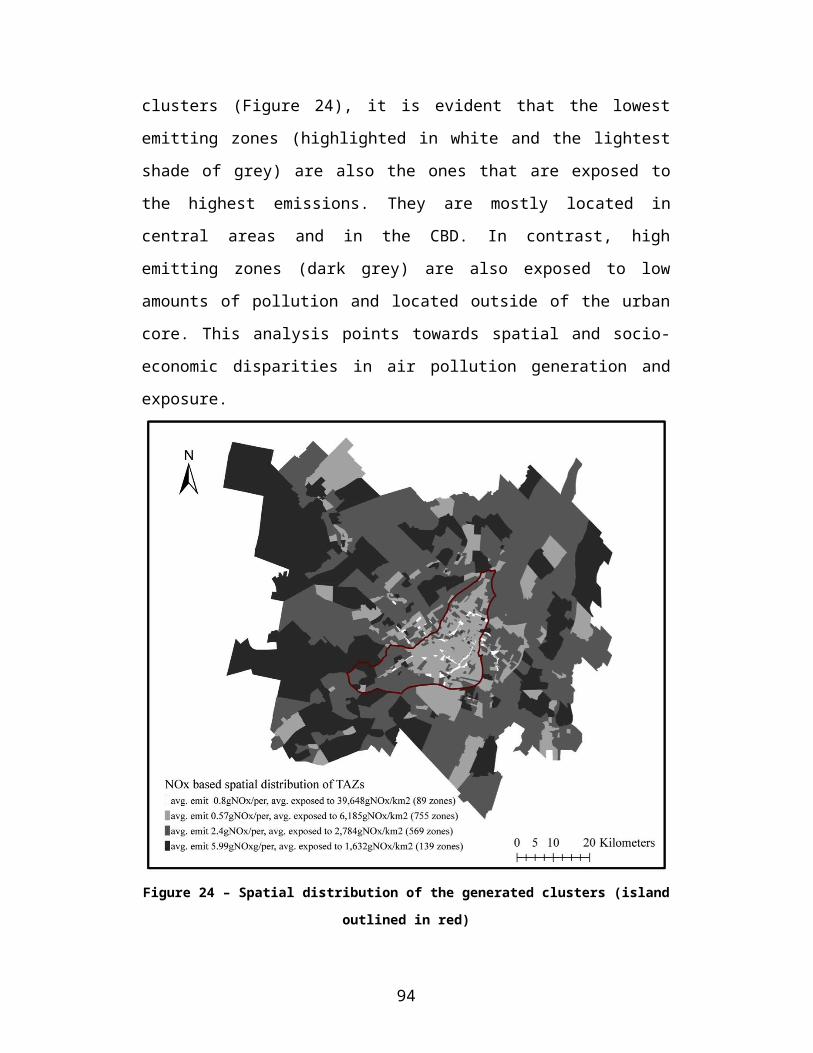
Environment, 61, 446-452.
Wheeler, A.J., Smith-Doiron, M., Xu, X., Gilbert, N.L., & Brook, J.R. (2008).
Intra-urban variability of air pollution in Windsor, Ontario – measurement
and modelling for human exposure assessment. Environmental Research,
106, 7–16.
Woodcock, J., Banister, D., Edwards, P., Prentice, A.M., and Roberts, I. (2007).
Energy and transport. The Lancet, 370, 1078-1088.
Xia, L., and Shao, Y. (2005). Modelling of traffic flow and air pollution emission
with application to Hong Kong Island. Environmental Modelling and
Software, 20, 1175-1188.
Zmirou, D., Gauvin, S., Pin, I., Momas, I., Sahraoui, F., Just, J. et al. (2004).
Traffic related air pollution and incidence of childhood asthma: results of
the Vesta case-control study. Journal of Epidemiology & Community
Health, 58, 18-23.
94