IZA DP No. 2870

Do You Receive a Lighter Prison SentenceBecause You Are a Woman? An Economic Analysisof Federal Criminal Sentencing Guidelines

Supriya SarnikarTodd SorensenRonald L. Oaxaca

DI

SC

US

SI

ON

PA

PE

R S

ER

IE

S

Forschungsinstitutzur Zukunft der ArbeitInstitute for the Studyof Labor

June 2007

Do You Receive a Lighter Prison Sentence Because You Are a Woman?

An Economic Analysis of Federal Criminal Sentencing Guidelines

Supriya Sarnikar Westfield State College

Todd Sorensen

University of Arizona and IZA

Ronald L. Oaxaca

University of Arizona and IZA

Discussion Paper No. 2870 June 2007

IZA

P.O. Box 7240 53072 Bonn

Germany

Phone: +49-228-3894-0 Fax: +49-228-3894-180

E-mail: iza@iza.org

Any opinions expressed here are those of the author(s) and not those of the institute. Research disseminated by IZA may include views on policy, but the institute itself takes no institutional policy positions. The Institute for the Study of Labor (IZA) in Bonn is a local and virtual international research center and a place of communication between science, politics and business. IZA is an independent nonprofit company supported by Deutsche Post World Net. The center is associated with the University of Bonn and offers a stimulating research environment through its research networks, research support, and visitors and doctoral programs. IZA engages in (i) original and internationally competitive research in all fields of labor economics, (ii) development of policy concepts, and (iii) dissemination of research results and concepts to the interested public. IZA Discussion Papers often represent preliminary work and are circulated to encourage discussion. Citation of such a paper should account for its provisional character. A revised version may be available directly from the author.

IZA Discussion Paper No. 2870 June 2007

ABSTRACT

Do You Receive a Lighter Prison Sentence Because You Are a Woman? An Economic Analysis of

Federal Criminal Sentencing Guidelines*

The Federal criminal sentencing guidelines struck down by the U.S. Supreme Court in 2005 required that males and females who commit the same crime and have the same prior criminal record be sentenced equally. Using data obtained from the United States Sentencing Commission’s records, we examine whether there exists any gender-based bias in criminal sentencing decisions. We treat months in prison as a censored variable in order to account for the frequent outcome of no prison time. Additionally, we control for the self-selection of the defendant into guilty pleas through use of an endogenous switching regression model. A new decomposition methodology is employed. Our results indicate that women receive more lenient sentences even after controlling for circumstances such as the severity of the offense and past criminal history. JEL Classification: J78, K14, K42 Keywords: discrimination, criminal justice, decomposition analysis,

limited dependent variable analysis Corresponding author: Ronald L. Oaxaca Department of Economics University of Arizona McClelland Hall, Room 401QQ Tucson, AZ 85721-0108 USA E-Mail: rlo@email.arizona.edu

* The authors gratefully acknowledge the helpful comments of participants at the 2006 Midwestern Economics Association meetings, the 2006 Western Economics Association meetings, and the 2006 WPEG conference at the University of Kent and of seminar participants at IZA.

Gender equity has been one of the major global social issues to emerge out of the

20th century. A major focus of economists in this regard is on disparate labor market

outcomes for men and women. Emphasis is placed on human capital explanations for

gender wage gaps though there is some scope for other explanations, such as Becker

taste-driven discrimination, statistical discrimination, and market power. Labor mar-

ket outcomes potentially a¤ect future criminal activities, and criminal activities can

a¤ect labor market outcomes. This paper examines the gender equity issue in the

criminal justice arena and notes that labor market outcomes and criminal justice

outcomes can be jointly determined. A popular perception in the criminal justice

system is that female criminal behavior is a less serious problem than male criminal

behavior. Detailed statistics compiled by the Bureau of Justice Statistics show that

women commit fewer o¤enses than men and substantially di¤erent types of o¤enses

than men. However, the statistics also reveal a rising trend in o¤enses committed

by females and an increase in the incarceration of females in recent years. Beyond

the labor market implications of gender equity in the criminal justice system there is

also a concern for allocative e¢ ciency regarding resources devoted to deterrence and

incarceration.

The Federal Sentencing Guidelines that arose out of the Sentencing Reform Act

of 1984 and that were subsequently struck down by the U.S. Supreme Court in 2005

(consolidated cases of United States v. Booker, No. 04-104, and United States v.

Fanfan, No. 04-105) required that males and females who commit the same crime and

have the same prior criminal record receive equal sentences. Critics of the sentencing

guidelines argue that women should be accorded separate treatment because females

who are caught in the criminal justice system �enter it due to circumstances that are

distinctly di¤erent from those of men�1. Others argue that gender is not a factor

1�Research on Women and Girls in the Justice System.� National Institute of Justice Report

(September 2000) at page iii. Available at http://www.ncjrs.gov/pd¢ les1/nij/180973.pdf.

2

that should enter into the sentencing decision. The Supreme Court in its split 5

to 4 decision argued that the mandatory guidelines violated the rights of criminal

defendants to have a jury rather than a judge decide if defendants had committed all

elements of a given crime. Consequently, the guidelines are only advisory to judges

who may increase the length of sentences if they determine that the circumstances

based on jury determination or admission of the defendant merit a longer prison

sentence (Chicago Daily Law Bulletin 27 December 2005). The 2005 decision created

some ambiguity in how far judges could stray from the now "advisory" sentencing

guidelines. Currently, the Supreme Court is considering a case in which a sentencing

judge departed from the guidelines, only to have an appellate court overrule the

judge�s sentencing decision. The decision the Supreme Court hands down in this case

may have as large an impact on the way sentences are given as the 2005 case2 (New

York Times Feb 20, 2007)

Whether the circumstances in which a crime is committed should be a consideration

in criminal justice is not a question that we propose to answer here. Rather, we

address the question of whether or not women do indeed receive more lenient sentences

despite the sentencing guidelines. The answer to this question is important to both

sides of the debate. Those in the justice system who favor equal treatment but

believe that women are let o¤ too lightly may be especially harsh when judging a

female accused of crime, while those who favor separate treatment of women but

believe that they are treated equally may be less stringent. Thus, perceptions of

unequal treatment, when they are not based on systematic study and sound facts,

may lead to actual inequality in the justice system. A systematic study of whether

bias actually exists is therefore not only necessary but timely given the rising trend

in o¤enses committed by women and the increase in female incarceration rates as

2The pending cases are Clairborne v. United States, No. 06-5618 and Rita v. United States, No.

06-5754.

3

evidenced by the data compiled by the Bureau of Justice Statistics. Further work

can begin to better tie the relationship between gender equity in the criminal justice

system with gender equity in the labor market.

An unpublished paper by Oaxaca and Sarnikar (2005) [henceforth OS] uses a rich

data set on sentencing outcomes from the United State Sentencing Commission to es-

timate separate logistic regressions for men and women, where the dependent variable

is a binary variable measuring whether or not convicted individuals received federal

prison time. While summary statistics from their data set show that females are less

likely to receive prison time than males, more sophisticated analysis can take account

of covariates that can explain some or all of the gender sentencing di¤erential.

In this paper, we consider outcomes from the sentencing process more broadly for a

sample of whites who were convicted while the mandatory sentencing guidelines were

still in e¤ect. Speci�cally, we look beyond the binary Prison/No-Prison outcome to a

continuous measure of prison sentence. Ideally, one would want to take into account

the fact that defendants must choose whether or not to plea bargain or to take their

chances in a trial. Given that we work with a sample of convicted individuals (we

do not have data on acquittals), we model the probability of whether the conviction

was the result of a trial versus a plea bargain. We treat sentences handed down due

to guilty pleas as outcomes from one regime, while sentences given to defendants

convicted in a trial are treated as outcomes from a separate regime. This approach

allows characteristics to be weighted di¤erently depending on the path to conviction.

One would expect that the average sentences of identical defendants facing identical

charges should be lower in the plea regime.3 In our data set, around 25% of all

criminal sentences involve no prison time. Because of this considerable mass point at

3 If the sentences were lighter in the trial regime it would be di¢ cult to believe that defendants

would ever do anything but plead not guilty, as this would generate a positive probability of facing

no sentence at all.

4

zero, it may be inappropriate to consider the distribution of sentencing outcomes to

be continuous. Also, the plea vs. trial regime is a choice variable for the defendant

so that we must account for self selection in our model. Accordingly, we treat the

outcome variable as a mixed discrete continuous variable. Therefore, our econometric

model is a censoring (Tobit) switching regression with endogenous switching, which

we estimate by full information maximum likelihood (FIML).

To measure how much of the male/female sentencing di¤erential can be attributed

to di¤erences in the characteristics of men and women, compared to how much of the

di¤erential can be explained by di¤erences in the weights applied to these character-

istics by judges, we develop a new decomposition. This decomposition builds upon

Neuman and Oaxaca (2004), which addresses the issue of selectivity in the context of

a Heckman sample selection model. We expand this analysis to decompose di¤eren-

tials in the switching regression model with censoring. Our approach takes account

of the fact that predicted outcome means will not generally match sample outcome

means because of the highly non-linear nature of the model.

Within our data set, the scarcity of observations on females and the preponderance

of observations in the plea regime conspire to leave us with an insu¢ cient sample

size to properly apply FIML to estimate the sentencing determination model sepa-

rately for females. In the decomposition developed here, we exploit an insight from

Oaxaca and Ransom (1994) that allows us to decompose the male-female regime and

sentencing di¤erentials without actually estimating the model for females. Rather

than comparing weights from a male only and female only model, we instead are

able to compare the estimated parameters from the model for males with parameters

estimated in a pooled model for males and females.

5

LITERATURE

Since the seminal work of Becker (1968), there has been a signi�cant amount of

research aimed at understanding the economics of crime. In the basic economic model

of crime, a rational individual decides whether or not to allocate his/her time to

criminal activity by comparing the expected net return from criminal activity to the

expected returns from legitimate activity. The expected net return to criminal activity

consists of the potential �nancial and psychic bene�ts (B) of committing the crime

minus the cost (C) of committing the crime. The cost to the individual of committing

the crime is determined as the product of the probability (p) of being caught by law

enforcement and the severity of the punishment (S). If the returns to legitimate labor

market activity is the wage (W), then a rational, risk-neutral individual will engage

in criminal activity only if B-pS > W. This static model therefore predicts that

criminal activity can be deterred by either increasing the probability of detection(p),

the severity of punishment(S) and/or the wage rate (W) in the labor market.

Economists have since subjected these theoretical predictions to empirical testing

using econometric models of varying degrees of sophistication. Ehrlich (1973) and

Levitt (1997) estimate the impact of increased law enforcement presence on crime

and �nd that increasing law enforcement e¤orts have the desired e¤ect of lowering

the incidence of crime. Ehrlich (1977) estimated the deterrence e¤ect of capital pun-

ishment on crime. Witte (1980) �nds that the deterrence e¤ect of higher legal wages

was small compared to the deterrence e¤ects of the severity and certainty of state

imposed penalties. Johnson, Kantor and Fishback (2007) study the e¤ect of social

insurance on crime rates. Block and Gerety (1995) reports on laboratory experiments

that examine di¤erences between the criminal population and the general population

in the relative responsiveness to the deterrence e¤ects of severity of punishment versus

the deterrence e¤ects of the certainty of punishment. The results showed that convicts

6

were more deterred by increases in the certainty of punishment whereas the student

subjects were more deterred by increases in the severity of punishment. Kuziemko

(2006) uses New York State�s reinstatement of the death penalty to identify the ef-

fect of capital punishment on plea bargaining outcomes. Freeman (1999), Grogger

(1998), and Gould, Weinberg and Mustard (2002) �nd that falling real wages were a

signi�cant determinant of increasing crime rates during the decades of the 1970s and

1980s.

The link between deterrence e¤orts and crime rates is an endogenous one. Deci-

sions to increase law enforcement e¤orts are often made in response to increasing crime

rates. Similarly, di¢ culty in �nding legitimate labor market employment might push

some individuals into criminal activity but the fact that an individual has engaged in

criminal activity also would lower that individual�s probability of �nding legitimate

employment. Myers (1983) investigates whether poor labor market prospects post-

release a¤ect the re-integration of ex-convicts into the mainstream. Using di¤erent

data sets, Myers �nds that better wages post-release signi�cantly reduced recidivism.

Witte and Reid (1980) also �nd that receiving a high wage on the �rst job after being

released from prison decreases recidivism and that the wage rate received by a prison

�releasee�depends mostly on the demand side characteristics such as the industry

and occupation rather than on the accumulated human capital of the �releasee�. Imai

and Krishna (2004) estimate a dynamic model of criminal behavior and show that

expected future adverse consequences in the labor market prove to be an e¤ective

deterrent to crime. Waldfogel (1994) estimated the e¤ects of conviction and impris-

onment on post-conviction income and employment probabilities and found that the

state-imposed sanctions were much smaller in comparison to the �market sanction�,

which he estimated as the income lost due to conviction and imprisonment. Also, the

�market sanction�was signi�cant only for those o¤enders who worked at jobs that

required much trust. Grogger (1995) used longitudinal data and concluded that the

7

strong negative correlation between arrests and subsequent labor market sanctions

that was found in earlier cross-sectional studies was largely due to unobserved char-

acteristics that in�uence both criminal and labor market behavior. Grogger (1995)

however does �nd that there are signi�cant negative consequences of arrests in the

labor market but that they are short-lived.

Consistent with the predictions of the economic model of crime, the Sentencing

Reform Act of 1984 (SRA 1984) increased the length of punishment for almost all

crimes, eliminated probation and reduced the possibility of parole for good behavior.

Kling (2006) estimates the e¤ect of this increased severity of punishment on labor

market prospects of criminals post-release. Kling �nds that there is no signi�cant

adverse e¤ect on employment or earnings of criminals due to longer incarceration

lengths and concludes that this may be because prison rehabilitation programs may

be o¤setting the loss of potential work experience and human capital depreciation

while in prison.

The sentencing guidelines formulated pursuant to the SRA 1984 aimed to provide

uniform sanctions for the same crime by eliminating gender, age, or racial disparities

in sentencing. While economists have studied the deterrence e¤ect of severity of pun-

ishment quite extensively, relatively little literature exists on the optimality and de-

sirability of uniform sentencing. Lott (1992) argues against uniform sentencing based

on the �nding that market sanctions in the form of lost incomes, opportunity costs

of imprisonment and the adverse impact of incarceration on labor market prospects

are disproportionately higher for individuals with higher incomes. Since the expected

total monetary penalty includes the reduction in legitimate earnings capability post

release, Lott argues that the state-imposed punishments should be proportionately

adjusted. Moreover, since mere conviction can restrict the post-conviction opportu-

nities for higher income individuals more severely than for lower skilled people, Lott

argues that in order to equalize the severity of punishment, higher income individuals

8

would have to be convicted much less frequently than low-income criminals. One

could argue that such equalization could be addressed by di¤erential sentence length.

However, the sentencing guidelines explicitly prohibited sentencing judges from con-

sidering factors such as the defendant�s socioeconomic status, race, sex, age, and

religion. The punishment was to be proportional to the severity of the crime and the

defendant�s criminal history alone. Judicial discretion to change the sentence based

on characteristics of the defendant was thus severely restricted under the guidelines.

Several studies in the criminology literature have examined gender and racial dis-

parities in sentencing prior to the formulation of sentencing guidelines. See Tonry

(1996) for a survey of these studies. Whether the guidelines have been successful in

reducing the disparity has also been studied extensively both in the criminology and

the law and economics literature. Anderson, Kling and Stith (1999), Kempf-Leonard

and Sample (2001) study sentencing disparities before and after the federal sentencing

guidelines. Mustard (2001) looks at racial and gender disparities in sentencing under

the federal guidelines and �nds that observed disparities in sentencing are mainly due

to the special circumstances when judges are allowed to depart from the guidelines

and not due to discriminatory tastes of judges. Schanzenbach (2005) estimates the

e¤ect of judicial demographics on sentencing outcomes and �nds that increasing the

proportion of female judges increases the gender disparity in sentencing and inter-

prets this as evidence that male judges are paternalistic and therefore lenient towards

female o¤enders.

Almost all of the studies mentioned infer gender-based discrimination in sentencing

from the statistically signi�cant coe¢ cient on a dummy variable indicating the gen-

der of the criminal o¤ender. Yet, sentencing discrepancies may be observed merely

because a judge takes into account extralegal circumstances of the defendant. If the

circumstances of male and female criminal defendants are substantially di¤erent, as

claimed by several authors, then the consideration of circumstances by judges may

9

appear as gender-based bias even when the judge exhibits no such discriminatory

tastes. Verdier and Zenou (2004) show that when there is statistical discrimination

in the labor market and everyone believes that blacks, for example, are more likely to

engage in criminal activity, then such beliefs lead to lower wages for blacks. When the

opportunity cost of a crime is thus lowered, such beliefs become self-ful�lling and lead

to higher crime rates among blacks. It is therefore important to thoroughly investi-

gate whether any bias actually exists in the criminal justice system since perceived

bias may itself lead to actual bias. Given the adverse labor market consequences of

incarceration, unequal treatment of men and women in the criminal justice system

may lead to unequal prospects for men and women in the labor market as well.

Our research design separates the e¤ect of di¤erences in circumstances from the

e¤ect of di¤erences in weights attached to circumstances by judges. If a judge attaches

di¤erent weights to the same circumstances of a male and a female o¤ender, then we

may attribute that to a gender-based bias. But if a judge attaches the same weights to

circumstances but on average awards di¤erent sentences to male and female o¤enders

then that di¤erence in sentencing might be due to di¤erences in circumstances of the

two defendants. Oaxaca and Sarnikar (2005) use decomposition analysis to investigate

whether there exists any leniency towards women in the binary decision of whether or

not to imprison a convicted person. The results of this decomposition show that the

di¤erences in characteristics explain more than 100% of the gender sentencing gap.

If, when determining whether or not to sentence a woman to prison, judges applied

the same weights on characteristics as they use for men, women would actually be

slightly less likely to face prison.

DATA

The data used in this study are obtained from the United States Sentencing Com-

mission�s data collection e¤orts and pertain to cases that terminated in convictions

10

over the period 1996-2002. The data set is available from the Federal Justice Resource

Statistics Center. In order to abstract from sentencing issues associated with race and

ethnicity, we have con�ned our attention to convicted white males and white females.

There were a total of 45,060 sentencing cases in our sample (37,104 cases for males

and 7,956 cases for women).

Table 1 presents a summary of the share of sentences involving no prison time.

Overall, a higher percentage of females receive no prison time upon conviction. This is

true for both the trial and guilty plea regimes. For both males and females, conviction

by a guilty plea is associated with a larger percentage of sentences involving no prison

time.

The variables reported in Table 2 are the ones we have constructed for use in our

sentence determination model. Both the measure of �nal o¤ense level and the criminal

history variable are set according to a �xed formula. To calculate the o¤ense level,

the case is assigned a base level for o¤ense and then adjusted for various aggravating

circumstances such as the use of a �rearm in the crime or obstruction of justice, or for

mitigating circumstances such as acceptance of responsibility. The criminal history

measure is a function of both the length of prior imprisonments and how recently these

sentences were given.4. While men on average are awarded longer prison sentences

(42 months) than women (17 months), the severity of their o¤enses as measured by

the �nal o¤ense level scores are greater on average than those of women. Also, men

on average have a higher past criminal history score than women. Convicted men are

on average two years older than convicted women and are more likely to have private

counsel. A higher percentage of men are college graduates (13% vs. 7%).

4For details on their construction of these variables, please see the following documents on the

USSC�s website:

http://www.ussc.gov/training/sent_ex_rob.pdf

http://www.ussc.gov/training/material.htm

11

In Table 3 we present summary statistics pertaining to the average length of sen-

tences imposed on both men and women in each of our sample years. Note that in

each year the average male sentence is more than twice that of the average female

sentence. If one were to only consider these summary statistics and no covariates, it

would appear that women receive considerably lighter sentences than do males, and

that this di¤erence is considerably greater in the trial regime. Overall and in the

trial regime, average male sentences generally declined over the sample period while

average female sentences actually rose. Average sentences in the plea regime tended

to rise for both males and females.

ECONOMETRIC MODEL

Below we describe the econometric methods used to estimate the necessary pa-

rameters to decompose the sentence di¤erentials. First, we describe the model we

use to decompose the sentence di¤erence into an explained portion (di¤erences in

characteristics) and an unexplained portion (di¤erences in weights).

Sentencing

In our data set, we observe the sentencing outcomes for defendants whose cases

reach the sentencing phase. Recall that there are two ways in which a defendant�s

case can reach the sentencing phase. While a signi�cant number of defendants faced

sentencing after being convicted by a jury, the most frequent way a defendant reached

the sentencing phase was by pleading guilty. Plea bargains reached with a prosecutor

are often the reason for this guilty plea; these defendants are sentenced under what

we call the plea regime. When a defendant pleads not guilty, but is convicted in a

trial, they are sentenced under the trial regime. We de�ne y as the months in prison

the defendant is sentenced to, X as the vector of the individual�s characteristics, and

12

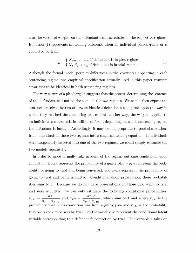
� as the vector of weights on the defendant�s characteristics in the respective regimes.

Equation (1) represents sentencing outcomes when an individual pleads guilty or is

convicted by trial:

yi =

�XPi�P + "Pi if defendant is in plea regimeXTi�T + "Ti if defendant is in trial regime.

(1)

Although the formal model permits di¤erences in the covariates appearing in each

sentencing regime, the empirical speci�cation actually used in this paper restricts

covariates to be identical in both sentencing regimes.

The very nature of a plea bargain suggests that the process determining the sentence

of the defendant will not be the same in the two regimes. We would then expect the

sentences received by two otherwise identical defendants to depend upon the way in

which they reached the sentencing phase. Put another way, the weights applied to

an individual�s characteristics will be di¤erent depending on which sentencing regime

the defendant is facing. Accordingly, it may be inappropriate to pool observations

from individuals in these two regimes into a single sentencing equation. If individuals

were exogenously selected into one of the two regimes, we could simply estimate the

two models separately.

In order to more formally take account of the regime outcome conditional upon

conviction, let �P represent the probability of a guilty plea, �T&C represent the prob-

ability of going to trial and being convicted, and �T&A represent the probability of

going to trial and being acquitted. Conditional upon prosecution, these probabil-

ities sum to 1. Because we do not have observations on those who went to trial

and were acquitted, we can only estimate the following conditional probabilities:

�PC =�P

�P + �T&Cand �TC =

�T&C�P + �T&C

; which sum to 1 and where �PC is the

probability that one�s conviction was from a guilty plea and �TC is the probability

that one�s conviction was by trial. Let the variable s� represent the conditional latent

variable corresponding to a defendant�s conviction by trial. The variable s takes on

13

a value of 1 if the defendant�s conviction is by trial, and a value of 0 if the defendant

enters a guilty plea. The vector index variable Zi is a set of variables a¤ecting this

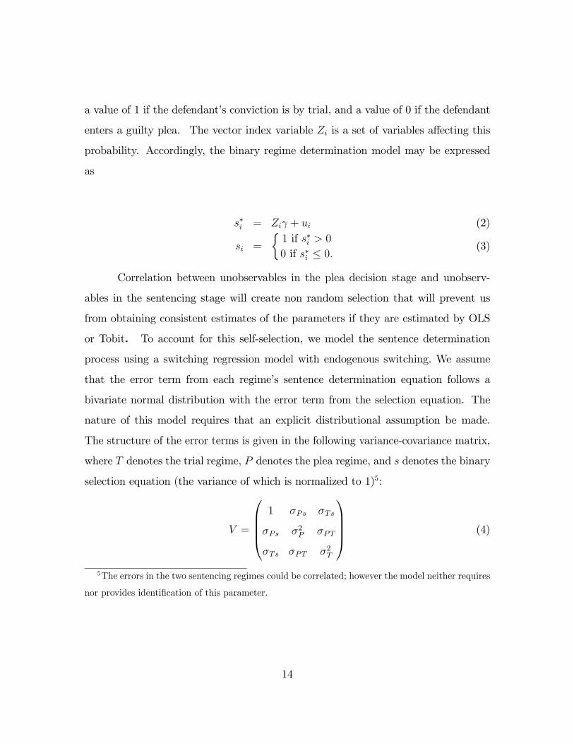
probability. Accordingly, the binary regime determination model may be expressed

as

s�i = Zi + ui (2)

si =

�1 if s�i > 00 if s�i � 0:

(3)

Correlation between unobservables in the plea decision stage and unobserv-

ables in the sentencing stage will create non random selection that will prevent us

from obtaining consistent estimates of the parameters if they are estimated by OLS

or Tobit. To account for this self-selection, we model the sentence determination

process using a switching regression model with endogenous switching. We assume

that the error term from each regime�s sentence determination equation follows a

bivariate normal distribution with the error term from the selection equation. The

nature of this model requires that an explicit distributional assumption be made.

The structure of the error terms is given in the following variance-covariance matrix,

where T denotes the trial regime, P denotes the plea regime, and s denotes the binary

selection equation (the variance of which is normalized to 1)5:

V =

0BBB@1 �Ps �Ts

�Ps �2P �PT

�Ts �PT �2T

1CCCA (4)

5The errors in the two sentencing regimes could be correlated; however the model neither requires

nor provides identi�cation of this parameter.

14

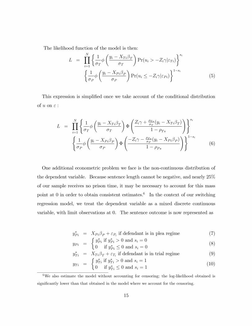
The likelihood function of the model is then:

L =NYi=1

�1

�T�

�yi �XTi�T

�T

�Pr(ui > �Zi j"Ti)

�si�1

�P�

�yi �XPi�P

�P

�Pr(ui � �Zi j"Pi)

�1�si(5)

This expression is simpli�ed once we take account of the conditional distribution

of u on " :

L =NYi=1

(1

�T�

�yi �XTi�T

�T

��

Zi +

�Ts�T(yi �XTi�T )

1� �Ts

!)si(1

�P�

�yi �XPi�P

�P

��

�Zi � �Ps

�P(yi �XPi�P )

1� �Ps

!)1�si(6)

One additional econometric problem we face is the non-continuous distribution of

the dependent variable. Because sentence length cannot be negative, and nearly 25%

of our sample receives no prison time, it may be necessary to account for this mass

point at 0 in order to obtain consistent estimates.6 In the context of our switching

regression model, we treat the dependent variable as a mixed discrete continuous

variable, with limit observations at 0. The sentence outcome is now represented as

y�Pi = XPi�P + "Pi if defendant is in plea regime (7)

yPi =

�y�Pi if y

�Pi > 0 and si = 0

0 if y�Pi � 0 and si = 0(8)

y�Ti = XTi�T + "Ti if defendant is in trial regime (9)

yTi =

�y�Ti if y

�Ti > 0 and si = 1

0 if y�Ti � 0 and si = 1(10)

6We also estimate the model without accounting for censoring; the log-likelihood obtained is

signi�cantly lower than that obtained in the model where we account for the censoring.

15

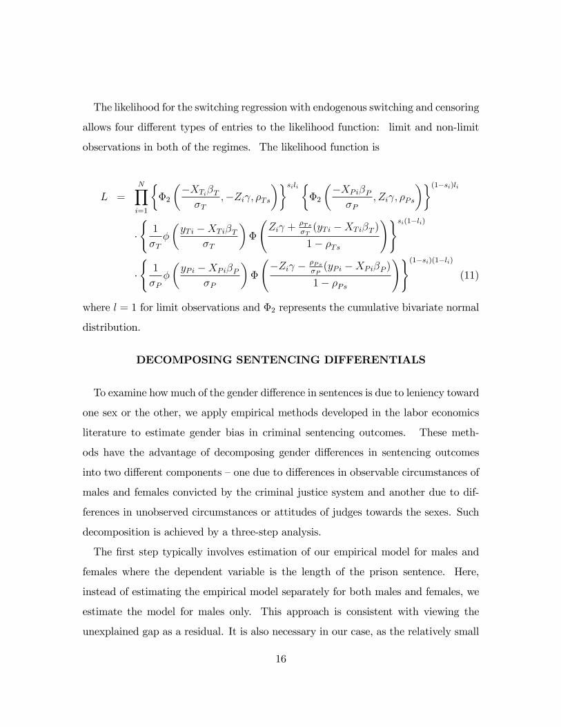
The likelihood for the switching regression with endogenous switching and censoring

allows four di¤erent types of entries to the likelihood function: limit and non-limit

observations in both of the regimes. The likelihood function is

L =

NYi=1

��2

��XTi�T�T

;�Zi ; �Ts��sili �

�2

��XPi�P�P

; Zi ; �Ps

��(1�si)li�(1

�T�

�yTi �XTi�T

�T

��

Zi +

�Ts�T(yTi �XTi�T )

1� �Ts

!)si(1�li)

�(1

�P�

�yPi �XPi�P

�P

��

�Zi � �Ps

�P(yPi �XPi�P )

1� �Ps

!)(1�si)(1�li)(11)

where l = 1 for limit observations and �2 represents the cumulative bivariate normal

distribution.

DECOMPOSING SENTENCING DIFFERENTIALS

To examine how much of the gender di¤erence in sentences is due to leniency toward

one sex or the other, we apply empirical methods developed in the labor economics

literature to estimate gender bias in criminal sentencing outcomes. These meth-

ods have the advantage of decomposing gender di¤erences in sentencing outcomes

into two di¤erent components �one due to di¤erences in observable circumstances of

males and females convicted by the criminal justice system and another due to dif-

ferences in unobserved circumstances or attitudes of judges towards the sexes. Such

decomposition is achieved by a three-step analysis.

The �rst step typically involves estimation of our empirical model for males and

females where the dependent variable is the length of the prison sentence. Here,

instead of estimating the empirical model separately for both males and females, we

estimate the model for males only. This approach is consistent with viewing the

unexplained gap as a residual. It is also necessary in our case, as the relatively small

16

number of female observations in the trial regime means that we are unable to identify

a number of parameters in an estimation of the model for females only. This approach

allows us to decompose the di¤erential without estimating the female weights, thus

circumventing the problem.

Our analysis departs from previous studies in the second step and adds greater

insight into the decision-making process that might lead to gender-based di¤erences

in criminal sentencing. In the second step, we predict the average sentence length

for females if they faced the male weights. In the third and �nal step, we use results

from the �rst two steps and decompose the di¤erences in length of sentences for

males and females into two components: one attributable to male-female di¤erences

in circumstances and a second attributable to unobserved di¤erences in attitudes of

judges towards the sexes and unobserved di¤erences in circumstances.

Decomposition methods such as the one described above were �rst developed in

labor market studies of gender and racial wage di¤erences [(Oaxaca 1973)] but have

not been used in studies of gender or racial bias in criminal sentencing decisions. Such

a method of estimating bias is valuable since it not only estimates any gender-based

di¤erences in sentencing outcomes but it also identi�es whether the observed bias

is due to gender di¤erences in circumstances or due to gender-based di¤erences in

weights attached to circumstances by judges.

In addition to the problems with identifying the female weights, we face two addi-

tional challenges which force us to expand beyond the Oaxaca (1973) decomposition.

The issue of selection bias in decompositions is addressed by Neuman and Oaxaca

(2004) in the context of a Heckit model. We are able to build o¤ of this work in the

decomposition we develop, as the Heckit is essentially a special case of an endogenous

switching regression model. Finally, we must account for the existence of the limit

observations in our data set.

17

Decomposing Sentencing Outcomes by Regime

First, consider the sentence determination equation for the trial regime:

y�Ti = XTi�T + "Ti if defendant is in the trial regime (12)

yTi =

�y�Ti if y

�Ti > 0; si = 1

0 if y�Ti � 0; si = 1(13)

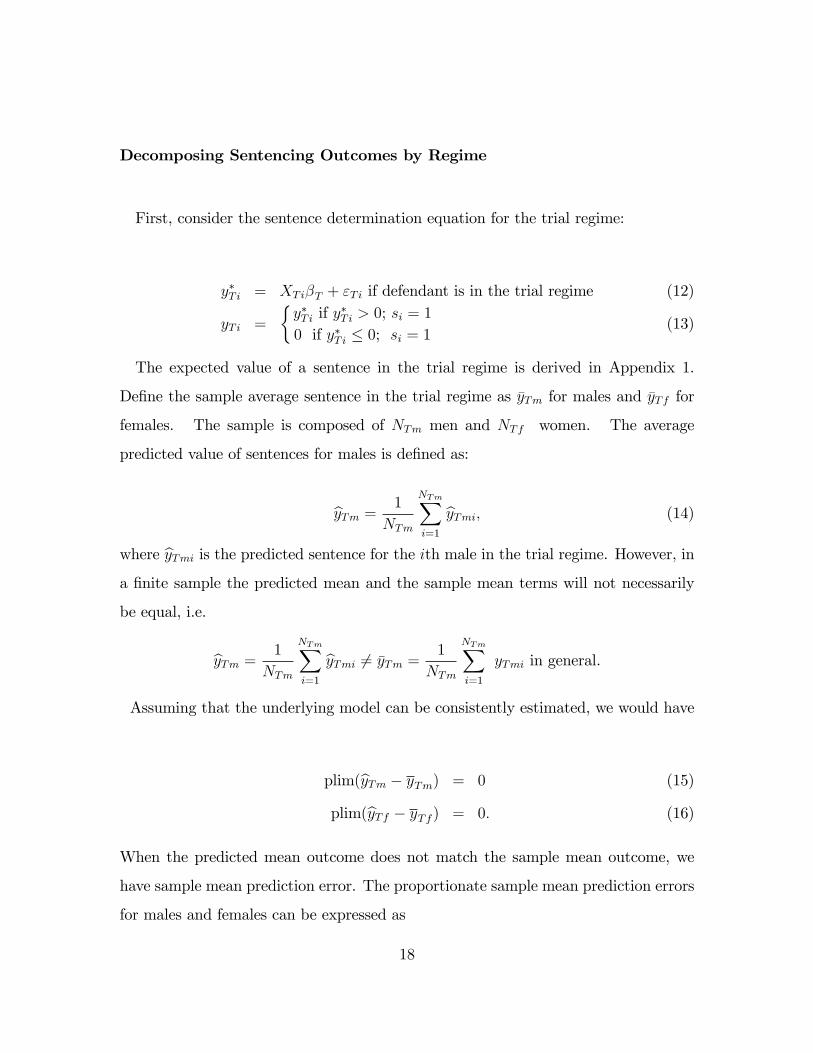
The expected value of a sentence in the trial regime is derived in Appendix 1.

De�ne the sample average sentence in the trial regime as �yTm for males and �yTf for

females. The sample is composed of NTm men and NTf women. The average

predicted value of sentences for males is de�ned as:

byTm = 1

NTm

NTmXi=1

byTmi; (14)

where byTmi is the predicted sentence for the ith male in the trial regime. However, ina �nite sample the predicted mean and the sample mean terms will not necessarily

be equal, i.e.

byTm = 1

NTm

NTmXi=1

byTmi 6= �yTm = 1

NTm

NTmXi=1

yTmi in general.

Assuming that the underlying model can be consistently estimated, we would have

plim(byTm � yTm) = 0 (15)

plim(byTf � yTf ) = 0: (16)

When the predicted mean outcome does not match the sample mean outcome, we

have sample mean prediction error. The proportionate sample mean prediction errors

for males and females can be expressed as

18

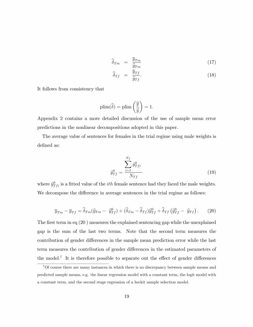
b�Tm =yTmbyTm (17)

b�Tf =yTfbyTf : (18)

It follows from consistency that

plim(b�) = plim�yby�= 1:

Appendix 2 contains a more detailed discussion of the use of sample mean error

predictions in the nonlinear decompositions adopted in this paper.

The average value of sentences for females in the trial regime using male weights is

de�ned as:

y0Tf =

NfXi=1

y0Tfi

NTf(19)

where y0Tfi is a �tted value of the ith female sentence had they faced the male weights.

We decompose the di¤erence in average sentences in the trial regime as follows:

yTm � yTf = b�Tm(byTm � by0Tf ) + (b�Tm � b�Tf )by0Tf + b�Tf �by0Tf � byTf� : (20)

The �rst term in eq (20 ) measures the explained sentencing gap while the unexplained

gap is the sum of the last two terms. Note that the second term measures the

contribution of gender di¤erences in the sample mean prediction error while the last

term measures the contribution of gender di¤erences in the estimated parameters of

the model.7 It is therefore possible to separate out the e¤ect of gender di¤erences

7Of course there are many instances in which there is no discrepancy between sample means and

predicted sample means, e.g. the linear regression model with a constant term, the logit model with

a constant term, and the second stage regression of a heckit sample selection model.

19

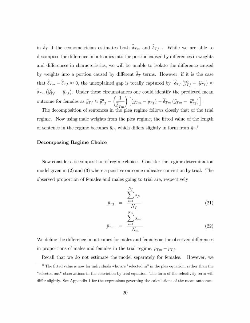
in �T if the econometrician estimates both b�Tm and b�Tf . While we are able to

decompose the di¤erence in outcomes into the portion caused by di¤erences in weights

and di¤erences in characteristics, we will be unable to isolate the di¤erence caused

by weights into a portion caused by di¤erent �T terms. However, if it is the case

that b�Tm � b�Tf � 0, the unexplained gap is totally captured by b�Tf �by0Tf � byTf� �b�Tm �by0Tf � byTf�. Under these circumstances one could identify the predicted meanoutcome for females as byTf � by0Tf � � 1b�Tm

�h�yTm � yTf

�� b�Tm �byTm � by0Tf�i :

The decomposition of sentences in the plea regime follows closely that of the trial

regime. Now using male weights from the plea regime, the �tted value of the length

of sentence in the regime becomes yP , which di¤ers slightly in form from yT .8

Decomposing Regime Choice

Now consider a decomposition of regime choice. Consider the regime determination

model given in (2) and (3) where a positive outcome indicates conviction by trial. The

observed proportion of females and males going to trial are, respectively

�pTf =

NfXi=1

sfi

Nf(21)

�pTm =

NmXi=1

smi

Nm(22)

We de�ne the di¤erence in outcomes for males and females as the observed di¤erences

in proportions of males and females in the trial regime, �pTm � �pTf .

Recall that we do not estimate the model separately for females. However, we

8 The �tted value is now for individuals who are "selected in" in the plea equation, rather than the

"selected out" observations in the conviction by trial equation. The form of the selectivity term will

di¤er slightly. See Appendix 1 for the expressions governing the calculations of the mean outcomes.

20

are still able to decompose the di¤erence in male and female outcomes into the por-

tion caused by di¤erences in characteristics and the portion caused by di¤erences in

weights. We go about these single model decompositions by decomposing di¤erentials

using only the estimated weights for males.

Here, we decompose the di¤erence in the propensity of males and females to be

convicted by trial regime using only male weights. Consider the regime determination

model estimated for males:

s�mi = Zmi m + ui (23)

smi =

�1 if s�mi > 00 if s�mi � 0

(24)

The estimated weights in this model allow us to obtain a predicted probability of

conviction by trial for each individual in the sample:

pTmi = �(Zmi m) (25)

We compute the average predicted probability by averaging the individual predicted

probabilities:

pTm =NmXi=1

�(Zmi m)

Nm(26)

Note that in the probit model, unlike the logit model, the average predicted prob-

ability of entering the trial regime will not necessarily equal the proportion of the

sample who do in fact enter the regime (for further work on the decomposition of

di¤erentials in the context of a probit model, see Fairly (2005) and Yun (1999)).

In practice the di¤erence is typically negligible. However, the selection probability

parameters in our model are obtained from FIML applied to the joint estimation of

the selection probability and sentencing equations. Hence, there is a need to scale the

mean predicted probabilities when conducting a decomposition of gender di¤erences

21

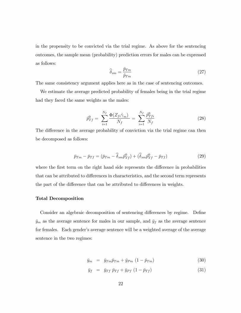
in the propensity to be convicted via the trial regime. As above for the sentencing

outcomes, the sample mean (probability) prediction errors for males can be expressed

as follows: b�sm = �pTmpTm

(27)

The same consistency argument applies here as in the case of sentencing outcomes.

We estimate the average predicted probability of females being in the trial regime

had they faced the same weights as the males:

p0Tf =

NfXi=1

�(Zfi m)

Nf=

NfXi=1

p0TfiNf

(28)

The di¤erence in the average probability of conviction via the trial regime can then

be decomposed as follows:

�pTm � �pTf = (�pTm � b�smp0Tf ) + (b�smp0Tf � �pTf ) (29)

where the �rst term on the right hand side represents the di¤erence in probabilities

that can be attributed to di¤erences in characteristics, and the second term represents

the part of the di¤erence that can be attributed to di¤erences in weights.

Total Decomposition

Consider an algebraic decomposition of sentencing di¤erences by regime. De�ne

�ym as the average sentence for males in our sample, and �yf as the average sentence

for females. Each gender�s average sentence will be a weighted average of the average

sentence in the two regimes:

�ym = �yTm�pTm + �yPm (1� �pTm) (30)

�yf = �yTf �pTf + �yPf (1� �pTf ) (31)

22

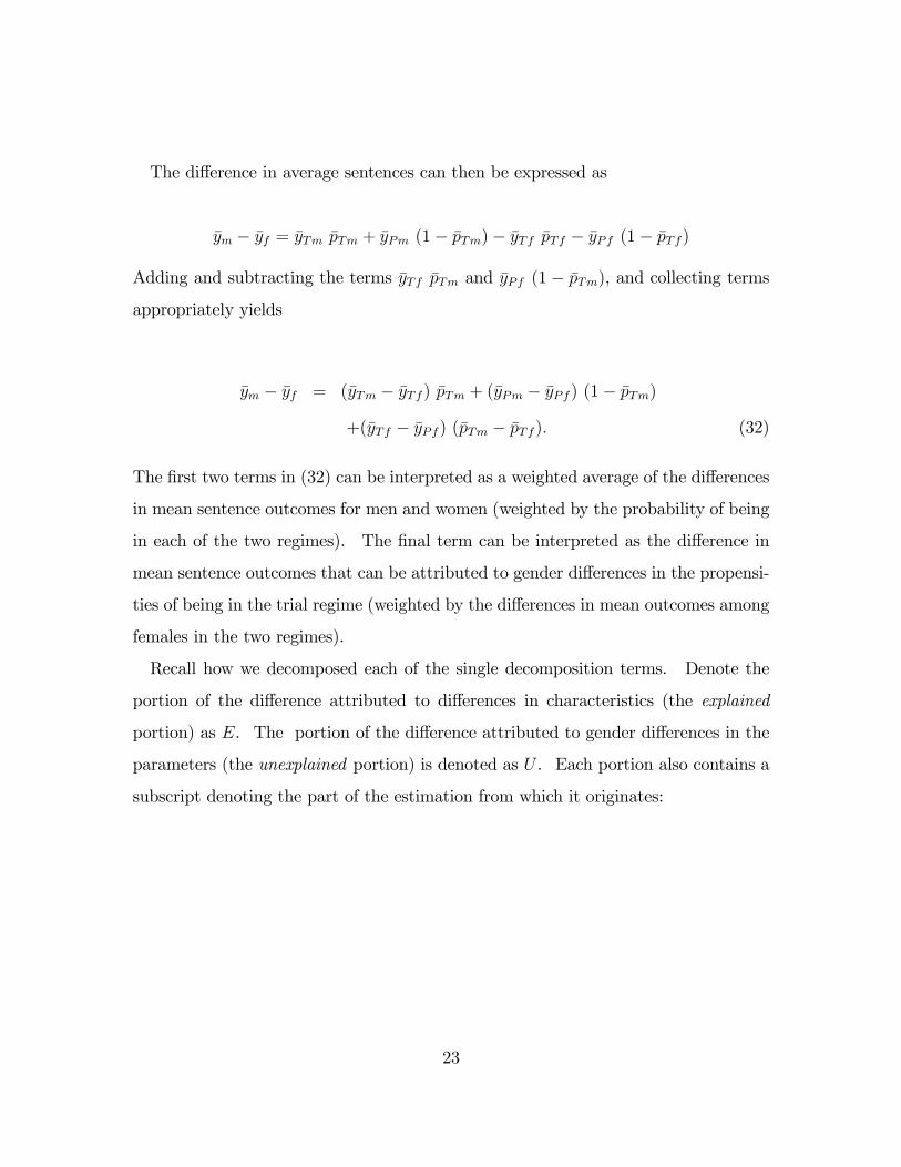
The di¤erence in average sentences can then be expressed as

�ym � �yf = �yTm �pTm + �yPm (1� �pTm)� �yTf �pTf � �yPf (1� �pTf )

Adding and subtracting the terms �yTf �pTm and �yPf (1 � �pTm), and collecting terms

appropriately yields

�ym � �yf = (�yTm � �yTf ) �pTm + (�yPm � �yPf ) (1� �pTm)

+(�yTf � �yPf ) (�pTm � �pTf ): (32)

The �rst two terms in (32) can be interpreted as a weighted average of the di¤erences

in mean sentence outcomes for men and women (weighted by the probability of being

in each of the two regimes). The �nal term can be interpreted as the di¤erence in

mean sentence outcomes that can be attributed to gender di¤erences in the propensi-

ties of being in the trial regime (weighted by the di¤erences in mean outcomes among

females in the two regimes).

Recall how we decomposed each of the single decomposition terms. Denote the

portion of the di¤erence attributed to di¤erences in characteristics (the explained

portion) as E. The portion of the di¤erence attributed to gender di¤erences in the

parameters (the unexplained portion) is denoted as U . Each portion also contains a

subscript denoting the part of the estimation from which it originates:

23

�yTm � �yTf =hb�Tm(byTm � by0Tf )i+ h(b�Tm � b�Tf )by0Tf + b�Tf �by0Tf � byTf�i

= ET + UT (33)

�yPm � �yPf =hb�Pm(byPm � by0Pf )i+ h(b�Pm � b�Pf )by0Pf + b�Pf �by0Pf � byPf�i

= EP + UP (34)

�pTm � �pTf = (�pTm � b�smp0Tf ) + (b�smp0Tf � �pTf )= Es + Us (35)

The decomposition of the overall gender sentencing gap can then be expressed as

�ym � �yf = [(ET + UT ) �pTm + (EP + UP ) (1� �pTm)]

+(�yTf � �yPf ) (Es + Us) (36)

= ET �pTm + EP (1� �pTm) + Es (�yTf � �yPf )| {z }E

+UT �pTm + UP (1� �pTm) + Us (�yTf � �yPf )| {z }U

;

where E is the total amount of the overall gender sentencing gap that is explained

by di¤erences in characteristics, and U is the total unexplained gap associated with

di¤erences in weights.

We note that a more straight forward total decomposition of the mean sentencing

di¤erences between men and women can be calculated as

�ym � �yf =��ym � �my0f

�+ (�my

0f � �yf ) (37)

where

y0f =

Pi

�p0Tfiy

0Tfi +

�1� p0Tfi

�y0Pfi

�Nf

and

�m =

�Pi [pTmiyTmi + (1� pTmi) yPmi]

Nm

��1

�ym

�:

24

In this decomposition y0f is the mean �tted overall sentence for females using the

male weights. Empirically, it turns out that both (36 ) and (37) yield virtually

identical values of the total explained and unexplained portions of the overall gender

sentencing gap. However, a shortcoming of the decomposition given by (37) is that

it obscures the sources of the overall gender sentencing gap revealed by the more

detailed decomposition given in (36).

RESULTS

Formal theory does not o¤er very much guidance on the actual speci�cation of the

regime selection and sentencing equations. The sentencing guidelines largely con�ned

federal court judges to considering only current o¤ense level and criminal history

when passing sentence. Speci�cally, the guidelines exclude race, sex, national origin,

creed, religion, and socioeconomic status. Furthermore, employment and family ties

and responsibilities are also not to be considered in awarding criminal sentences.

With only limited exception, age and education are not supposed to be relevant

for sentencing decisions. Judges are permitted to award lighter prison sentences to

elderly defendants. Since we have data on these various potential factors, we are able

to empirically determine the extent to which they turn out to in�uence sentences

because of, or despite, the guidelines. The variables that appear jointly in the regime

selection and sentencing equations are indicators for females (in the pooled sample),

education, marital status, the circuit court district, and year while the continuous

variables appearing jointly pertain to prior criminal history, number of dependents,

and age. An indicator for U.S. citizenship appears in the regime selection equation

but not in the sentencing equations. While judges should not take into account the

nationality of a defendant when determining her sentence, citizenship should serve

as a proxy for this defendant�s knowledge of and experience with the U.S. criminal

justice system; we would expect risk averse individuals with less knowledge of how

25

this process works to be less likely to take their chances in a trial rather than striking

a plea bargain deal. An indicator for a defendant�s �ne being waived appears in the

sentencing equation but not in the regime selection equation. This variable serves

as a crude proxy for income. Also, a cubic polynomial function of the severity of

the �nal o¤ense level appears in the sentencing equations but are excluded from the

regime selection equation. Both the �ne variable and the �nal criminal o¤ense level

variables are not determined at the time that the individual makes the decision about

going to trial. Given that defendants do not have perfect foresight, these variables

should determine the �nal sentence given but not a¤ect the plea decision.

Although our data span both cases and years, it is not treated as a panel. The data

are available as separate cross-sections by case for each year. Each case corresponds to

all prosecutions ending in convictions of an individual in the given year and the total

prison time awarded. While it is theoretically possible for an individual to appear in

more than one year�s cross-section, we suspect that this is not very common. Among

males the average prison sentence is 3.5 years over a period of 7 years. This does

not leave much time for multiple year convictions unless o¤enses are committed while

the individual is in prison. In the case of females the average prison sentence is 1.4

years over the period of our study. This would allow for multiple year convictions

except that the crime rate is still much lower for females. Female cases account for

just under 18% of the total number of cases in our data set.

To get a sense of whether or not there may be favoritism towards women, we �rst

estimate our model on a pooled sample of males and females, including an indicator

variable for whether the observation is that of a female o¤ender. In Table 4 we present

parameter estimates from this pooled sample of males and females The estimated

coe¢ cient on the female indicator variable is negative and signi�cant in the selection

equation, indicating that women are less likely to obtain their convictions via the trial

regime, where average sentences are higher. More educated and married individuals

26

are more likely to obtain their convictions through trial rather than through guilty

pleas. Being a U.S. citizen is associated with a lower probability of obtaining one�s

conviction via trial as opposed to a guilty plea. The chances that one would obtain

their conviction via trial rather than via a guilty plea rise with age until around 73

years after which the trial regime probability declines. The circuit court district in

which the conviction took place does a¤ect the probability of conviction via trial vs.

guilty plea. The year indicators (where 2002 is the omitted reference group) suggest

that the probability of obtaining conviction via trial relative to guilty plea steadily

declined over time. A more extensive past criminal history was positively associated

with conviction by trial vs. a guilty plea. Having a private defense counsel has a

statistically signi�cant negative impact on the probability of conviction by trial.

The estimated coe¢ cients on the female gender indicator are negative and statisti-

cally signi�cant in both sentencing regimes, but they are of a greater magnitude (in

absolute value) in the trial regime. Even before we allow all weights to di¤er by gen-

der, this indicates that women may receive lighter sentences than men. This would

seemingly violate the sentencing guidelines. Contrary to the guidelines, marital sta-

tus and number of dependents do a¤ect prison sentences, but only in the plea regime.

Married defendants receive shorter sentences in the plea regime. Having more depen-

dents leads to shorter sentences in the plea regime. Age and education exhibit some

e¤ect on sentences though ordinarily these are not considered relevant by the guide-

lines. Sentence length rises with age and peaks at 69 years if one is convicted in the

trial regime and peaks at 29 years in the plea regime. Although the guidelines permit

lighter sentences for the elderly, a peak of 29 years in the plea regime and the strong

signi�cance of the age terms in the trial regime would not seem to be entirely con-

sistent with the guidelines. Education appears to lower sentences in the plea regime

and raise them in the trial regime. Those who have been convicted and had �nes

waived receive longer sentences in the plea regime. If this variable adequately proxies

27

incomes of the defendants, then it would seem that poorer defendants receive longer

sentences in the plea regime. As expected the extent of a defendant�s criminal history

and severity of current �nal criminal o¤ense contribute to longer prison sentences in

both regimes. The signs and magnitudes of the linear, quadratic, and cubic terms

jointly imply that, for all relevant values of the variable, as the severity of the crime

for which one is convicted increases, sentence length increases at an increasing rate.

Having a private defense counsel lowered prison sentences in both conviction regimes.9

Similar to the case with conviction regime selection, the circuit court district in which

the conviction took place does a¤ect sentence lengths. The estimated coe¢ cients on

the time indicator variables reveal that, ceteris paribus, sentence length had been

declining over time in the trial regime while rising in the plea regime. Estimates of

the correlations between the conviction regime error and the sentencing regime errors

suggest that unobservables in the selection equation are negatively correlated with

unobservables in the trial sentencing equation and positively correlated with unob-

servables in the plea regime. Roughly speaking, this means that those who are more

likely to select into the conviction by trial regime can expect shorter sentences in the

trial regime and longer sentences in the plea regime. While this is a sensible result,

one potential problem is that the estimated correlation coe¢ cient between the regime

selection equation error term and the plea regime sentencing error term is close to

the boundary value of 1. It is probably the case that this extreme estimate of the

correlation coe¢ cient is caused by the fact that ninety �ve percent of the sample

9If the choice of defense counsel and the conviction regime are jointly determined, then the choice

of defense counsel would be endogenous in the model. Accordingly, we estimate a model to determine

if the decision to be represented by a private attorney is jointly determined with regime choice. By

estimating the model with a bivariate probit, we can test for this possible correlation in the two

error terms related to these decisions. Our estimation �nds the error term correlation coe¢ cient to

be insigni�cant, suggesting that the coe¢ cient on the defense counsel variable in the main model is

consistently estimated.

28

represent convictions via guilty pleas.

In Table 5 we report the FIML estimates based on just the male sample. Since

the results for males are qualitatively the same as those for the pooled sample, we

do not separately discuss these estimates. The major purpose behind estimating the

model separately for males is to provide us with the necessary parameter estimates

to compute the decomposition of gender di¤erences in prison sentences.

Decomposition results are reported in Tables 6 through 8. We begin with Table 6

which presents mean sentencing outcomes by regime and regime selection di¤erences

as well as predicted outcomes using estimated male weights. On average men are

awarded nearly 25 more months of prison than women. This varies by sentencing

regime. For those convicted by trial, men received an average of 69 more months of

prison than women. Among those who plead guilty, men received an average of almost

22 more months of prison time than women. A higher percentage of men than women

received their convictions via trial vs. a guilty plea, 5.5% vs. 3.5%. From the �tted

(predicted mean) sentences for males, we are able to calculate the proportionate mean

sample prediction errors. The most accurate prediction corresponds to the plea regime

which is the one into which the vast majority of the cases fall. The last column of

Table 6 reports the predicted outcomes for females using the FIML estimated weights

for men and are comparable to the calculated �tted values for men reported in the

next to the last column in Table 6. For the actual decompositions, the proportionate

mean prediction errors for men are applied to the predicted outcomes for women

obtained using the estimated male weights. The �gures in Table 6 clearly imply that

if females had faced the same sentence determination process as men, they would

have experienced longer prison sentences in each regime, though still less than those

of men, and would have had a higher propensity to have received their convictions

from the trial regime as opposed to the plea regime.

Our decompositions of gender sentencing di¤erences in each regime and gender

29

di¤erences in conviction regime probabilities are reported in Table 7. Di¤erences in

the female mean characteristics explain 46% of the gender sentencing di¤erential in

the trial regime and 66% of the sentencing di¤erential in the plea regime. We observe

that of the 69 month sentencing gap that favors women in the trial regime, nearly 38

months of the gap cannot be accounted for by gender di¤erences in circumstances.

Of the 22 month sentencing gap that favors women in the plea regime, 7 months of

the gap cannot be accounted for by gender di¤erences in circumstances. Only about

21% of the 2.1 percentage point gender gap in the propensity to obtain conviction in

the trial regime can be explained by gender di¤erences in characteristics. Females are

also less likely to be sentenced in the trial regime, though their characteristics suggest

they would actually be more likely to be sentenced in this regime if they were to face

the male weights (though still less likely than males).

In Table 8 we parse out the components that add to the overall gender sentencing

di¤erence across both conviction regimes. These components weight the explained

and unexplained portions of the sentencing gaps in each regime by the probabilities

of being in each regime and gender di¤erences in these probabilities. Of the nearly

25 month overall gender sentencing gap favoring women, 3.8 months (15.4%) arises

from gender sentencing di¤erences in the trial regime. Gender sentencing di¤erences

in the plea regime account for a little over 20 months (81.6%) of the overall gap. The

remainder of less than one month (3.0%) is accounted for by gender di¤erences in

conviction regime probabilities. Overall, the explained portion of the gap accounts for

about 15.4 months (62.7%) of the total gender sentencing di¤erence. This leaves about

9.5 months (38.3%) that cannot be explained by gender di¤erences in circumstances.

Table 8 disaggregates the explained and unexplained portions of the overall sentencing

gap by contributions from each sentencing regime and sentencing regime probabilities.

The plea regime accounts for the largest contribution to the overall explained gap (13.5

months or 87.6%) and to the overall unexplained gap (6.8 months or 72.0%). In fact

30

the largest single component of the constituent parts of the overall gender sentencing

gap is the 13.5 month explained gap from the plea regime which accounts for 54.0%

of the overall advantage of women in awarded sentences.

CONCLUSION

Unlike any studies in the literature so far, our study separates observed gender dif-

ferences in sentencing into two di¤erent components �one attributable to di¤erences

in circumstances of male and female criminal defendants, and the second attributable

to di¤erences in attitudes of sentencing judges towards male and female defendants

and the di¤erences due to unobservable characteristics of the male and female defen-

dants. Our model takes account of the joint determination of sentences by regime

and conviction regime selection as well as censoring occasioned by sentences that do

not involve prison time. We are able to determine the role of gender di¤erences in

selection regime probabilities. Such decomposition provides a better insight into the

decision-making process of sentencing judges. Knowing whether judges consider ex-

tralegal circumstances in their decision making is important, but knowing how they

consider extralegal circumstances is useful to policy makers in deciding how to re-

form sentencing guidelines to ensure equal treatment. This study not only examines

whether judges consider extralegal circumstances but if they do, it asks whether they

attach the same weight to circumstances of males and females. Even in light of the

Supreme Court�s decision in 2005 to strike down the Federal Sentencing Guidelines,

our results may o¤er some guidance as to what to expect now that judges are less

constrained in imposing sentences.

We �nd that women receive prison sentences that average a little over 2 years

less than those awarded to men. Even after controlling for circumstances such as

the severity of the o¤ense and past criminal history, women receive more lenient

sentences. Approximately 9.5 months of the female advantage cannot be explained

31

by gender di¤erences in individual circumstances. In other words if women faced the

same sentencing structure as men, women would on average receive 15.4 months less

prison time than men rather than 24.9 months less prison time. Most of the gender

gap arises from convictions via guilty pleas, which account for the vast majority of

the convictions observed in our data. Besides gender, we �nd evidence that judges

took into account factors such as family circumstances which are expressly prohibited

from consideration when awarding sentences.

One should bear in mind that our data permit us to examine only the end stage of

the criminal justice system. A more comprehensive treatment would take account of

the fact that before arriving at the judge for sentencing, a defendant must also pass

through a jury or possible plea bargain with a prosecutor. Before reaching this stage,

other groups, such as the police and the prosecution, have the potential to create bias

in the criminal justice system. Future work will focus on separating out di¤erential

outcomes layer by layer, as well as making explicit the impact of gender bias in the

criminal justice system on gender di¤erences in labor market outcomes.

32

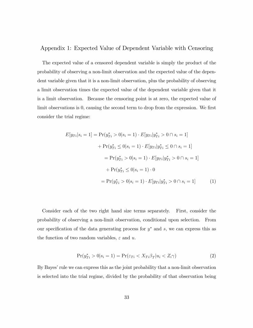
Appendix 1: Expected Value of Dependent Variable with Censoring

The expected value of a censored dependent variable is simply the product of the

probability of observing a non-limit observation and the expected value of the depen-

dent variable given that it is a non-limit observation, plus the probability of observing

a limit observation times the expected value of the dependent variable given that it

is a limit observation. Because the censoring point is at zero, the expected value of

limit observations is 0, causing the second term to drop from the expression. We �rst

consider the trial regime:

E[yTijsi = 1] = Pr(y�Ti > 0jsi = 1) � E[yTijy�Ti > 0 \ si = 1]

+ Pr(y�Ti � 0jsi = 1) � E[yTijy�Ti � 0 \ si = 1]

= Pr(y�Ti > 0jsi = 1) � E[yTijy�Ti > 0 \ si = 1]

+ Pr(y�Ti � 0jsi = 1) � 0

= Pr(y�Ti > 0jsi = 1) � E[yTijy�Ti > 0 \ si = 1] (1)

Consider each of the two right hand size terms separately. First, consider the

probability of observing a non-limit observation, conditional upon selection. From

our speci�cation of the data generating process for y� and s, we can express this as

the function of two random variables, " and u.

Pr(y�Ti > 0jsi = 1) = Pr("Ti < XTi�T jui < Zi ) (2)

By Bayes�rule we can express this as the joint probability that a non-limit observation

is selected into the trial regime, divided by the probability of that observation being

33

in the trial regime. This term can then be expressed using values from the cumulative

normal and cumulative bivariate normal distributions.

Pr(y�Ti > 0jsi = 1) =Pr( "Ti

�T< XTi�T

�T\ ui < Zi )

Pr(ui < Zi )

=�2(

XTi�T�T

; Zi ; �sT )

�(Zi ): (3)

Finally, we must consider the expected value of the dependent variable, given that

it is a non-limit observation in the trial regime. Recall that non-limit observations

take on the value

E[yTijy�Ti > 0 \ si = 1] = E[y�Tijy�Ti > 0 \ si = 1]

= E[y�Tijy�Ti > 0 \ s�i > 0]

= E[y�Tij"Ti�T

<XTi�T�T

\ ui < Zi ] : (4)

This expected value appears similar to the expected value of the dependent variable

in the main equation of the Heckit model: it is truncated by the draw for the error

term in the selection equation. It also appears similar to the expected value of the

dependent variable in the Tobit model: it is truncated by the draw for the error term

in the main equation. This incidence of "double truncation" however, is substantially

more complex than the single truncation in either the Tobit or the Heckit. We derive

it for our model based on page 72 of Johnson and Kotz (1972):

E[yTijy�Ti > 0 \ si = 1] =XTi�T

�2(XTi�T�T

; Zi ; �sT )

�(�Tf�(

�XTi�T�T

)�(�1p1� �2sT

[�Zi � ��XTi�T�T

])

+ �sT�(�Zi )�(�1p1� �2sT

[�XTi�T � �(�Zi )]))

(5)

34

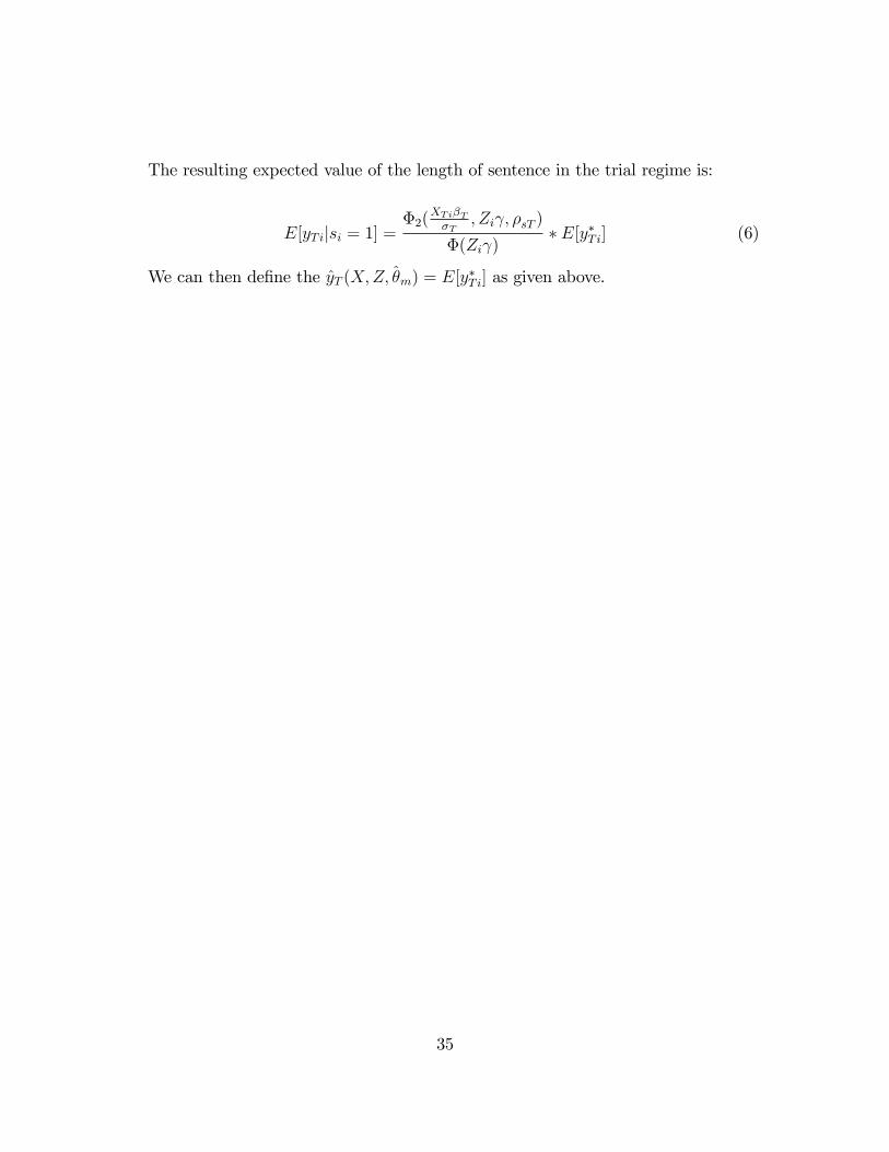
The resulting expected value of the length of sentence in the trial regime is:

E[yTijsi = 1] =�2(

XTi�T�T

; Zi ; �sT )

�(Zi )� E[y�Ti] (6)

We can then de�ne the yT (X;Z; �m) = E[y�Ti] as given above.

35

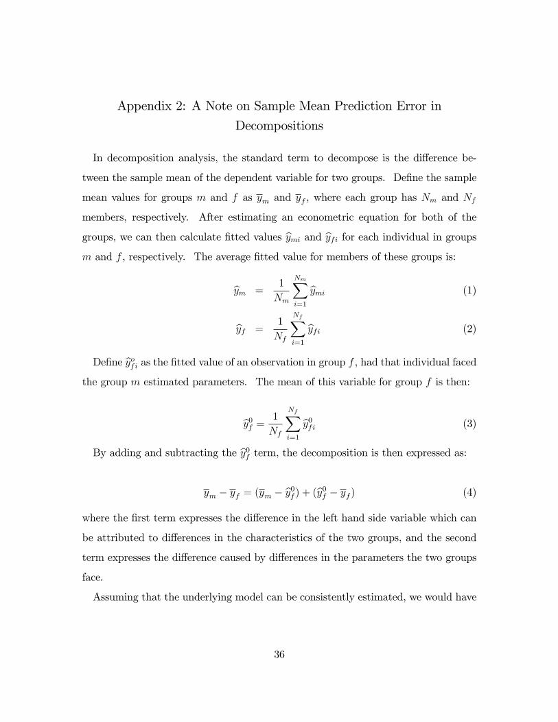
Appendix 2: A Note on Sample Mean Prediction Error in

Decompositions

In decomposition analysis, the standard term to decompose is the di¤erence be-

tween the sample mean of the dependent variable for two groups. De�ne the sample

mean values for groups m and f as ym and yf , where each group has Nm and Nf

members, respectively. After estimating an econometric equation for both of the

groups, we can then calculate �tted values bymi and byfi for each individual in groupsm and f , respectively. The average �tted value for members of these groups is:

bym =1

Nm

NmXi=1

bymi (1)

byf =1

Nf

NfXi=1

byfi (2)

De�ne byofi as the �tted value of an observation in group f , had that individual facedthe group m estimated parameters. The mean of this variable for group f is then:

by0f = 1

Nf

NfXi=1

by0fi (3)

By adding and subtracting the by0f term, the decomposition is then expressed as:ym � yf = (ym � by0f ) + (by0f � yf ) (4)

where the �rst term expresses the di¤erence in the left hand side variable which can

be attributed to di¤erences in the characteristics of the two groups, and the second

term expresses the di¤erence caused by di¤erences in the parameters the two groups

face.

Assuming that the underlying model can be consistently estimated, we would have

36

plim(bym � ym) = 0 (5)

plim(byf � yf ) = 0 (6)

However, in a �nite sample, the by and y terms will not necessarily be equal. We canexpress the sample mean prediction error in the model as follows:

ym = b�mbym (7)

yf = b�fbyf (8)

It follows from consistency that

plim(b�) = plim ��yby�= 1

The decomposition can now be expressed as:

ym � yf = (b�mbym � byof ) + (byof � b�fbyf ) (9)

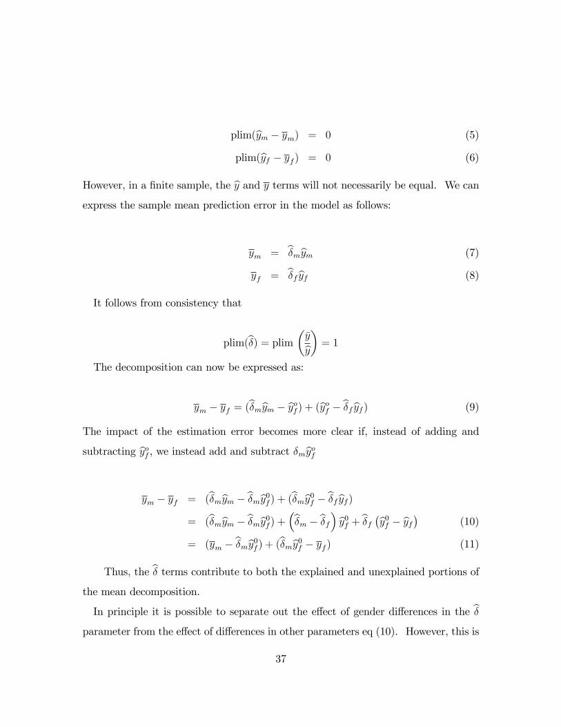
The impact of the estimation error becomes more clear if, instead of adding and

subtracting byof , we instead add and subtract �mbyofym � yf = (b�mbym � b�mby0f ) + (b�mby0f � b�fbyf )

= (b�mbym � b�mby0f ) + �b�m � b�f� by0f + b�f �by0f � byf� (10)

= (ym � b�mby0f ) + (b�mby0f � yf ) (11)

Thus, the b� terms contribute to both the explained and unexplained portions ofthe mean decomposition.

In principle it is possible to separate out the e¤ect of gender di¤erences in the b�parameter from the e¤ect of di¤erences in other parameters eq (10). However, this is

37

only feasible if the econometrician estimates both the b�m and b�f terms. In our case,we lack su¢ cient data to identify the weights in the model for females. Consequently,

we only are able to decompose the di¤erence in mean outcomes into the portion caused

by di¤erences in weights and di¤erences in characteristics according to eq (11).

38

REFERENCES

Anderson, James M., Je¤rey R. Kling, and Kate Stith, �Measuring Interjudge Sen-

tencing Disparity: Before and after the Federal Sentencing Guidelines,�Journal

of Law and Economics, 1999, 42, 271�298.

Becker, Gary, �Crime and Punishment: an Economic Approach,� Journal of Political

Economy, 1968, 76, 169�217.

Block, Michael K. and Vernon E. Gerety, �Some Experimental Evidence on Di¤er-

ences Between Student and Prisoner Reactions to Monetary Penalties and Risk,�

Journal of Legal Studies, 1995, 24, 123�138.

Chicago Daily Law Bulletin, Law Bulletin Publishing Company, 27 December 2005.

Defendants Sentenced Under the Guidelines During Fiscal Year 2001:

SC01OUT, Washington, D.C.: Bureau of Justice Statistics, Federal Justice

Statistics Program, 2001.

Ehrlich, I, �Participation in Illegitimate Activities: a Theoretical and Empirical Investi-

gation,�Journal of Political Economy, 1973, 81, 521�565.

, �Capital Punishment and Deterrence: Some Further Thoughts and Additional Ev-

idence,�Journal of Political Economy, 1977, 85, 741�788.

Fairly, Robert W., �An Extension of the Blinder-Oaxaca Decomposition Technique to

Logit and Probit Models,�Journal of Economic and Social Measurement, 2005,

30, 305�316.

Freeman, Richard B, �Why do so Many Young American Men Commit Crimes and

What Might we do about it?,�Journal of Economic Perspectives, 1999, 10, 25�

42.

39

Gould, Eric D., Bruce A. Weinberg, and David B. Mustard, �Crime Rates and

Local Labor Market Opportunities in the United States: 1979-1997,�Review of

Economics and Statistics, 2002, 84, 45�61.

Greene, William H., Econometric Analysis, 3rd edition, New Jersey: Prentice-Hall,

2003.

Grogger, Je¤rey, �The E¤ect of Arrests on the Employment and Earnings of Young

Men,�Quarterly Journal of Economics, 1995, 110, 51�71.

, �Market Wages and Youth Crime,�Journal of Labor Economics, 1998, 16, 756�791.

Imai, Susumu and Kala Krishna, �Employment, Deterrence and Crime in a Dynamic

Model,�International Economic Review, 2004, 45, 845�872.

Johnson, Norman L. and Samuel Kotz, Distributions in Statistics: Continuous Mul-

tivariate Distributions, New York: John Wiley and Sons, 1972.

Johnson, Ryan S., Shawn Kantor, and Price V. Fishback, �Striking at the Roots

of Crime: the Impact of Social Welfare Spending on Crime During the Great

Depression,�NBER Working Paper, 2007, No.12825.

Kempf-Leonard, Kimberly and Lisa L. Sample, �Have Federal Sentencing Guidelines

Reduced Severity? An Examination of one Circuit,� Journal of Quantitative

Criminology, 2001, 17, 111�144.

Kling, Je¤rey, �Incarceration Length, Employment and Earnings,�The American Eco-

nomic Review, 2006, 96, 863�876.

Kuziemko, Illyana, �Does the Threat of the Death Penalty A¤ect Plea Bargaining

in Murder Cases? Evidence from New York�s 1995 Reinstatement of Capital

Punishment,�American Law and Economics Review, 2006, 8, 116�142.

40

Levitt, Steven D., �Using Electoral Cycles in Police Hiring to Estimate the E¤ect of

Police on Crime,�American Economic Review, 1997, 87, 270�290.

Lott, John R. Jr., �An Attempt at Measuring the Total Monetary Penalty from Drug

Convictions: The Importance of an Individual�s Reputation,� The Journal of

Legal Studies, jan 1992, 21 (1), 159�187.

Mustard, D.B., �Racial, Ethnic, and Gender Disparities in Sentencing: Evidence from

the U.S. Federal Courts,�Journal of Law and Economics, 2001, 44, 285 �314.

Myers, Samuel L. Jr., �Estimating the Economic Model of Crime: Employment Versus

Punishment E¤ects,� The Quarterly Journal of Economics, feb 1983, 98 (1),

157�166.

Neuman, Shoshana and Ronald L. Oaxaca, �Wage Decompositions with Selectivity-

Corrected Wage Equations: a Methodological Note,� Journal of Economic In-

equality, 2004, 2, 3�10.

New York Times, Justices to Revisit Thorny Issue of Sentencing Guidelines in First

Case After Recess, Feb 20, 2007, Section A, 15.

Oaxaca, Ronald L., �Male-Female Wage Di¤erentials in Urban Labor Markets,�Inter-

national Economic Review, 1973, 14, 693�709.

and Michael R. Ransom, �On Discrimination and the Decomposition of Wage

Di¤erentials,�Journal of Econometrics, 1994, 61, 5�21.

and Supriya Sarnikar, �Do Females Receive Lenient Sentences Despite the Federal

Sentencing Guidelines?,�Mimeo, 2005.

Schanzenbach, M., �Racial and Sex Disparities in Prison Sentences: the E¤ect of

District-Level Judicial Demographics,�Journal of Legal Studies, 2005, 34, 57�92.

41

Tonry, Michael, Sentencing Matters, Oxford: Oxford University, 1996.

Verdier, Thierry and Yves Zenou, �Racial Beliefs, Location, and the Causes of

Crime,�International Economic Review, 2004, 45, 731�760.

Waldfogel, Joel, �The E¤ect of Criminal Conviction on Income and the Trust �Reposed

in the Workmen,�The Journal of Human Resources, 1994, 29, 62�81.

Witte, Ann D. and Pamela A. Reid, �An Exploration of the Determinants of Labor

Market Performance for Prison Releasees,�Journal of Urban Economics, 1980,

8, 313�329.

Witte, Ann Dryden, �Estimating the Economic Model of Crime with Individual Data,�

The Quarterly Journal of Economics, 1980, 94, 57�84.

Yun, Myeong-Su, �Generalized Selection Bias and the Decomposition of Wage Di¤er-

entials,�IZA Discussion Paper, 1999, Number 69.

42

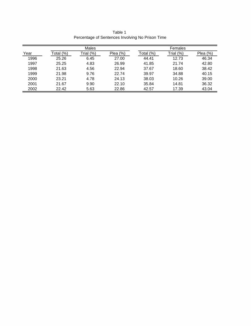
Year Total (%) Trial (%) Plea (%) Total (%) Trial (%) Plea (%)1996 25.26 6.45 27.00 44.41 12.73 46.341997 25.25 4.83 26.99 41.85 21.74 42.801998 21.63 4.56 22.94 37.67 18.60 38.421999 21.98 9.76 22.74 39.97 34.88 40.152000 23.21 4.78 24.13 38.03 10.26 39.002001 21.67 9.90 22.10 35.84 14.81 36.322002 22.42 5.63 22.86 42.57 17.39 43.04

Males Females

Table 1 Percentage of Sentences Involving No Prison Time

Variable Description Mean Std. Dev Mean Std. Dev Mean Std. DevTOTALMONTHS Length of prison sentence in months 37.27 73.12 41.67 78.03 16.76 37.07REGIME Indicator for trial regime 0.05 0.22 0.06 0.23 0.03 0.18FEMALE Indicator for female 0.18 0.38 0.00 0.00 1.00 0.00FINEWAIV Indicator of fine being waived 0.84 0.37 0.83 0.38 0.87 0.34HISCHOOL Indicator for high school education 0.24 0.43 0.23 0.42 0.28 0.45GED Indicator for general equivalency diploma 0.13 0.34 0.14 0.34 0.11 0.32SOMECOLL Indicator for some college attended 0.26 0.44 0.25 0.43 0.29 0.45COLLGRAD Indicator for a college degree or higher 0.12 0.32 0.13 0.33 0.07 0.26NUMDEPEN Number of dependents 1.13 1.41 1.13 1.44 1.09 1.29MARRD Indicator for married or cohabiting 0.26 0.44 0.26 0.44 0.25 0.43CITIZN Indicator for US citizen 0.95 0.21 0.95 0.22 0.97 0.16DEFENSEP Indicator for private counsel 0.36 0.48 0.37 0.48 0.30 0.46XCRHISSR Final criminal history category 2.11 1.60 2.23 1.66 1.57 1.16CRIMHIS1 Final criminal history category =1 0.58 0.49 0.54 0.50 0.74 0.44CRIMHIS2 Final criminal history category =2 0.12 0.32 0.12 0.33 0.09 0.29CRIMHIS3 Final criminal history category=3 0.13 0.33 0.13 0.34 0.10 0.29CRIMHIS4 Final criminal history category =4 0.06 0.24 0.07 0.25 0.03 0.17CRIMHIS5 Final criminal history category =5 0.04 0.19 0.04 0.20 0.02 0.13CRIMHIS6 Final criminal history category =6 0.08 0.27 0.09 0.29 0.03 0.16XFOLSOR Final offense level 16.80 8.30 17.37 8.35 14.11 7.51XFOLSOR2 Final offense level squared 351.02 325.02 371.49 332.24 255.55 269.16XFOLSOR3 Final offense level cubed 8507.77 11499.56 9140.23 11899.77 5558.17 8832.43AGE Age of defendant 37.74 11.14 38.08 11.22 36.16 10.59AGE2 Age of defendant squared 1548.66 888.58 1576.29 900.04 1419.79 820.88CIRC1 Circuit indicators 0.03 0.16 0.03 0.17 0.02 0.14CIRC2 Circuit indicators 0.11 0.31 0.12 0.32 0.08 0.27CIRC3 Circuit indicators 0.04 0.21 0.05 0.21 0.04 0.19CIRC4 Circuit indicators 0.05 0.21 0.05 0.21 0.05 0.21CIRC5 Circuit indicators 0.10 0.30 0.10 0.30 0.12 0.32CIRC6 Circuit indicators 0.08 0.28 0.08 0.27 0.09 0.29CIRC7 Circuit indicators 0.04 0.20 0.04 0.20 0.04 0.20CIRC8 Circuit indicators 0.08 0.27 0.08 0.27 0.09 0.29CIRC9 Circuit indicators 0.27 0.44 0.27 0.44 0.28 0.45CIRC10 Circuit indicators 0.05 0.23 0.05 0.22 0.06 0.24CIRC11 Circuit indicators 0.14 0.35 0.14 0.35 0.13 0.34

Overall Males Females

Table 2Variable Definitions and Summary Statistics

1996 Year indicators 0.13 0.33 0.13 0.33 0.12 0.331997 Year indicators 0.13 0.34 0.14 0.34 0.13 0.341998 Year indicators 0.13 0.34 0.13 0.34 0.14 0.351999 Year indicators 0.14 0.35 0.14 0.34 0.15 0.362000 Year indicators 0.14 0.35 0.14 0.35 0.15 0.352001 Year indicators 0.15 0.36 0.15 0.36 0.15 0.362002 Year indicators 0.17 0.37 0.17 0.38 0.16 0.36

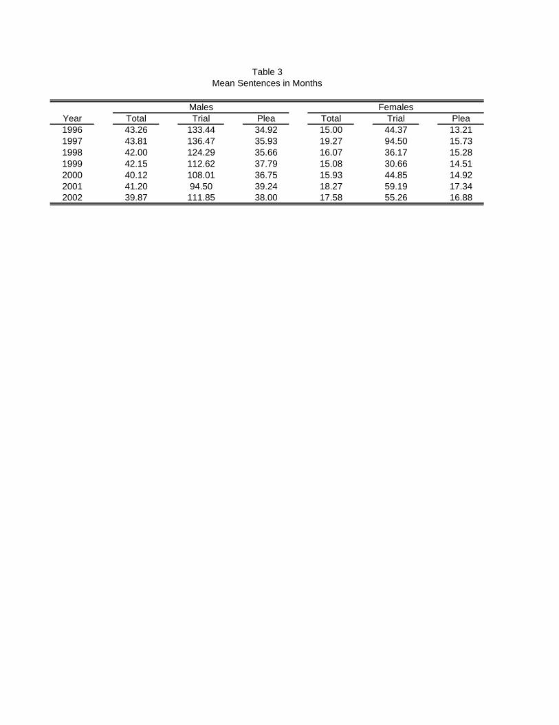
Year Total Trial Plea Total Trial Plea1996 43.26 133.44 34.92 15.00 44.37 13.211997 43.81 136.47 35.93 19.27 94.50 15.731998 42.00 124.29 35.66 16.07 36.17 15.281999 42.15 112.62 37.79 15.08 30.66 14.512000 40.12 108.01 36.75 15.93 44.85 14.922001 41.20 94.50 39.24 18.27 59.19 17.342002 39.87 111.85 38.00 17.58 55.26 16.88

Table 3Mean Sentences in Months

Males Females

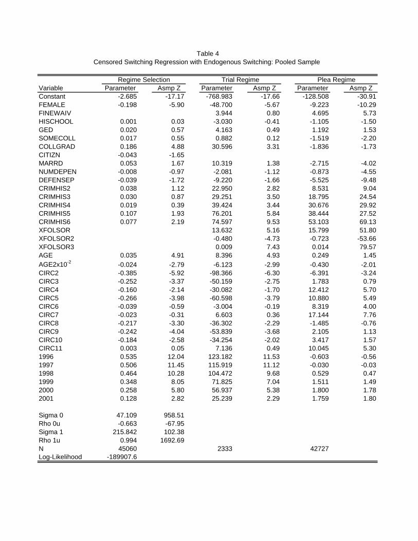
Variable Parameter Asmp Z Parameter Asmp Z Parameter Asmp ZConstant -2.685 -17.17 -768.983 -17.66 -128.508 -30.91FEMALE -0.198 -5.90 -48.700 -5.67 -9.223 -10.29FINEWAIV 3.944 0.80 4.695 5.73HISCHOOL 0.001 0.03 -3.030 -0.41 -1.105 -1.50GED 0.020 0.57 4.163 0.49 1.192 1.53SOMECOLL 0.017 0.55 0.882 0.12 -1.519 -2.20COLLGRAD 0.186 4.88 30.596 3.31 -1.836 -1.73CITIZN -0.043 -1.65MARRD 0.053 1.67 10.319 1.38 -2.715 -4.02NUMDEPEN -0.008 -0.97 -2.081 -1.12 -0.873 -4.55DEFENSEP -0.039 -1.72 -9.220 -1.66 -5.525 -9.48CRIMHIS2 0.038 1.12 22.950 2.82 8.531 9.04CRIMHIS3 0.030 0.87 29.251 3.50 18.795 24.54CRIMHIS4 0.019 0.39 39.424 3.44 30.676 29.92CRIMHIS5 0.107 1.93 76.201 5.84 38.444 27.52CRIMHIS6 0.077 2.19 74.597 9.53 53.103 69.13XFOLSOR 13.632 5.16 15.799 51.80XFOLSOR2 -0.480 -4.73 -0.723 -53.66XFOLSOR3 0.009 7.43 0.014 79.57AGE 0.035 4.91 8.396 4.93 0.249 1.45AGE2x10-2 -0.024 -2.79 -6.123 -2.99 -0.430 -2.01CIRC2 -0.385 -5.92 -98.366 -6.30 -6.391 -3.24CIRC3 -0.252 -3.37 -50.159 -2.75 1.783 0.79CIRC4 -0.160 -2.14 -30.082 -1.70 12.412 5.70CIRC5 -0.266 -3.98 -60.598 -3.79 10.880 5.49CIRC6 -0.039 -0.59 -3.004 -0.19 8.319 4.00CIRC7 -0.023 -0.31 6.603 0.36 17.144 7.76CIRC8 -0.217 -3.30 -36.302 -2.29 -1.485 -0.76CIRC9 -0.242 -4.04 -53.839 -3.68 2.105 1.13CIRC10 -0.184 -2.58 -34.254 -2.02 3.417 1.57CIRC11 0.003 0.05 7.136 0.49 10.045 5.301996 0.535 12.04 123.182 11.53 -0.603 -0.561997 0.506 11.45 115.919 11.12 -0.030 -0.031998 0.464 10.28 104.472 9.68 0.529 0.471999 0.348 8.05 71.825 7.04 1.511 1.492000 0.258 5.80 56.937 5.38 1.800 1.782001 0.128 2.82 25.239 2.29 1.759 1.80

Sigma 0 47.109 958.51Rho 0u -0.663 -67.95Sigma 1 215.842 102.38Rho 1u 0.994 1692.69N 45060 2333 42727Log-Likelihood -189907.6

Table 4Censored Switching Regression with Endogenous Switching: Pooled Sample

Regime Selection Trial Regime Plea Regime

Variable Parameter Asmp Z Parameter Asmp Z Parameter Asmp ZConstant -2.638 -15.64 -767.458 -15.67 -128.041 -26.57FINEWAIV 3.340 0.60 5.149 5.52HISCHOOL 0.017 0.51 -1.423 -0.17 -1.611 -1.88GED 0.036 0.94 7.070 0.75 1.172 1.32SOMECOLL 0.025 0.77 1.778 0.21 -1.885 -2.37COLLGRAD 0.171 4.18 26.557 2.58 -1.521 -1.28CITIZN -0.042 -1.52MARRD 0.055 1.60 11.390 1.35 -3.354 -4.30NUMDEPEN -0.006 -0.70 -1.706 -0.83 -0.948 -4.33DEFENSEP -0.049 -1.96 -11.229 -1.80 -6.532 -9.74CRIMHIS2 0.033 0.89 22.167 2.42 8.394 7.75CRIMHIS3 0.041 1.13 32.000 3.49 19.239 21.88CRIMHIS4 0.035 0.71 43.492 3.50 31.494 27.17CRIMHIS5 0.113 1.94 78.039 5.39 38.609 24.59CRIMHIS6 0.077 2.11 76.024 9.01 53.490 61.44XFOLSOR 11.693 3.94 15.581 43.19XFOLSOR2 -0.404 -3.54 -0.699 -44.14XFOLSOR3 0.008 5.97 0.014 65.83AGE 0.034 4.46 8.507 4.43 0.185 0.94AGE2x10-2 -0.024 -2.64 -6.336 -2.76 -0.343 -1.40CIRC2 -0.397 -5.80 -103.768 -6.08 -6.478 -2.89CIRC3 -0.258 -3.26 -52.720 -2.63 1.005 0.39CIRC4 -0.166 -2.10 -33.349 -1.71 12.327 4.94CIRC5 -0.278 -3.89 -61.521 -3.49 9.425 4.14CIRC6 -0.074 -1.06 -9.518 -0.53 7.088 2.98CIRC7 -0.034 -0.43 4.737 0.24 15.882 6.31CIRC8 -0.246 -3.52 -42.872 -2.44 -1.560 -0.69CIRC9 -0.259 -4.08 -57.704 -3.59 1.188 0.56CIRC10 -0.176 -2.33 -30.395 -1.63 2.539 1.01CIRC11 -0.013 -0.21 4.682 0.29 9.672 4.481996 0.538 11.14 126.383 10.40 -1.064 -0.851997 0.514 10.70 120.490 10.17 -0.825 -0.681998 0.481 9.72 111.016 8.99 -0.272 -0.211999 0.357 7.65 75.419 6.58 1.409 1.192000 0.257 5.34 55.756 4.69 1.362 1.162001 0.128 2.62 24.521 1.99 1.539 1.36

Sigma 0 49.543 858.88Rho 0u -0.692 -72.20Sigma 1 224.546 93.54Rho 1u 0.994 1535.52N 37104 2057 35047Log-Likelihood -163499.9

Regime Selection Trial Regime Plea Regime

Table 5Censored Switching Regression with Endogenous Switching: Males

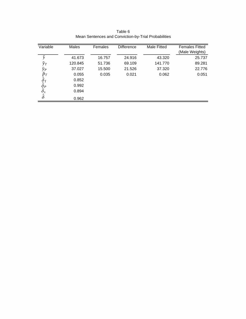
Variable Males Females Difference Male Fitted Females Fitted (Male Weights)

41.673 16.757 24.916 43.320 25.737 120.845 51.736 69.109 141.770 89.281

37.027 15.500 21.526 37.320 22.7760.055 0.035 0.021 0.062 0.0510.8520.9920.894

0.962

Mean Sentences and Conviction-by-Trial ProbabilitiesTable 6

yyT

pT

s

yP

P

T

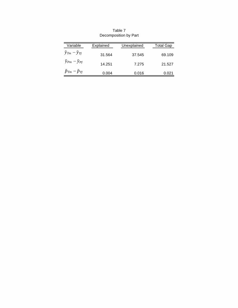
Variable Explained Unexplained Total Gap

31.564 37.545 69.109

14.251 7.275 21.527

0.004 0.016 0.021

Table 7Decomposition by Part

yTm − yTf

yPm − yPf

pTm − pTf

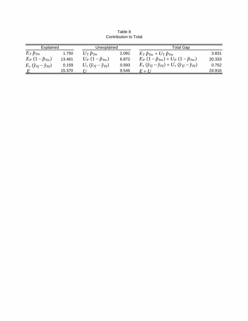
1.750 2.081 3.831 13.461 6.872 20.333 0.159 0.593 0.752 15.370 9.546 24.916

Table 8Contribution to Total

Explained Unexplained Total GapET pTm

Es yTf − yPfE

UT pTm

Us yTf − yPfU

ET pTm UT pTm

Es yTf − yPf Us yTf − yPfE U

EP 1 − pTm UP 1 − pTm EP 1 − pTm UP 1 − pTm