do value-added estimates add value? accounting for
TRANSCRIPT

29
American Economic Journal: Applied Economics 3 (July 2011): 29–54http://www.aeaweb.org/articles.php?doi=10.1257/app.3.3.29
Models of learning often assume that a child’s achievement persists between grades—what a child learns today largely stays with her tomorrow. Yet recent
research suggests that treatment effects measured by test scores fade rapidly, both in randomized interventions and observational studies. Thomas J. Kane and Douglas O. Staiger (2008); Brian A. Jacob, Lars Lefgren, and David P. Sims (2010); and Jesse Rothstein (2010) find that teacher effects dissipate by between 50 and 80 percent over 1 year. The same pattern holds in several studies of supplemental education programs in developed and developing countries. Janet Currie and Duncan Thomas (1995) document the rapid fade-out of Head Start’s impact in the United States, and Paul Glewwe, Nauman Ilias, and Michael Kremer (2010) and Abhijit V. Banerjee et al. (2007) report on education experiments in Kenya and India, where over 70 percent of the 1-year treatment effect is lost after an additional year. Low persistence may in fact be the norm rather than the exception. It appears to be a central feature of learning.
* Andrabi: Department of Economics, Pomona College, 425 N. College Ave., Claremont, CA 91711 (e-mail: [email protected]); Das: Development Research Group, The World Bank, 1818 H Street, NW, Washington, DC 20433 and The Center for Policy Research, New Delhi (e-mail: [email protected]); Khwaja: John F. Kennedy School of Government, Harvard University, 79 JFK Street, Cambridge, MA 02138, BREAD and National Bureau of Economic Research (e-mail: [email protected]); Zajonc: John F. Kennedy School of Government, Harvard University, 79 JFK Street, Cambridge, MA 02138 (e-mail: [email protected]). We are grateful to Alberto Abadie, Chris Avery, David Deming, Pascaline Dupas, Brian Jacob, Dale Jorgenson, Elizabeth King, Karthik Muralidharan, David McKenzie, Rohini Pande, Lant Pritchett, Jesse Rothstein, Douglas Staiger, Tara Vishwanath, an anonymous referee, and seminar participants at Harvard, NEUDC, and BREAD for helpful comments on drafts of this paper. This research was funded by grants from the Poverty and Social Impact Analysis and Knowledge for Change Program Trust Funds and the South Asia region of the World Bank. The findings, interpretations, and conclusions expressed here are those of the authors and do not necessarily represent the views of the World Bank, its Executive Directors, or the governments they represent.
† To comment on this article in the online discussion forum, or to view additional materials, visit the article page at http://www.aeaweb.org/articles.php?doi=10.1257/app.3.3.29.
Do Value-Added Estimates Add Value? Accounting for Learning Dynamics†
By Tahir Andrabi, Jishnu Das, Asim Ijaz Khwaja, and Tristan Zajonc*
This paper illustrates the central role of persistence in estimating and interpreting value-added models of learning. Using data from Pakistani public and private schools, we apply dynamic panel meth-ods that address three key empirical challenges: imperfect per-sistence, unobserved heterogeneity, and measurement error. Our estimates suggest that only one-fifth to one-half of learning persists between grades and that private schools increase average achieve-ment by 0.25 standard deviations each year. In contrast, value-added models that assume perfect persistence yield severely downward estimates of the private school effect. Models that ignore unobserved heterogeneity or measurement error produce biased estimates of per-sistence. (JEL I21, J13, O15)
ContentsDo Value-Added Estimates Add Value? Accounting for Learning Dynamics† 29
I. Empirical Learning Framework 31A. Addressing Child-Level Heterogeneity: Dynamic Panel Approaches to the Education Production Function 33B. Addressing Measurement Error 35C. Relationship to a Difference-in-Differences Strategy 35II. Data 36III. Results 39A. Cross-Sectional and Graphical Results 39B. OLS and Dynamic Panel Value-Added Estimates 44C. Robustness Checks 47IV. Conclusion 48Appendix: Additional Estimation Strategies 50A. System GMM 50B. Attrition Corrected Estimators 51References 53

30 AMErIcAn EcOnOMIc JOUrnAL: APPLIEd EcOnOMIcs JULy 2011
Low persistence has critical implications for commonly used program evalua-tion strategies that rest heavily on assumptions about or estimation of persistence. Using primary data on public and private schools in Pakistan, this paper addresses the challenges to value-added evaluation strategies posed by imperfect persistence of achievement, heterogeneity in learning, and measurement error in test scores. We find that ignoring any of these learning dynamics biases estimates of persistence and can dramatically affect estimates of the value-added of private schools.
To fix concepts, consider a simple model of learning, y it * = α T it + β y i,t−1 * + η i + υ it , where y it * is child true (unobserved) achievement in period t, T it is the treatment or program effect in period t, and η i is unobserved student ability that speeds learning each period. We refer to β, the parameter that links achievement across periods, as persistence. The canonical restricted value-added or gain-score model assumes that β = 1 (for examples, see Eric A. Hanushek 2003). When β < 1, achievement exhib-its conditional mean reversion. Estimates of the treatment or program effect, α, that assume β = 1 will be biased if the baseline achievement of the treatment and control groups differs and persistence is imperfect. This has led many researchers to advocate leaving lagged achievement on the right-hand side. However, doing so is not entirely straightforward; if estimated by OLS, omitted heterogeneity that speeds learning, η i , will generally bias β upward, and any measurement error in test scores y i,t−1 that proxy true achievement y i,t−1 * will bias β downward. Both the estimate of persistence β and the treatment effect α may remain biased when estimated by standard methods.
To address these concerns, we use three years of data on a panel of children to jointly estimate β and the treatment effect α using techniques from the dynamic panel literature (Manuel Arellano and Bo Honoré 2001; Arellano 2003). There are several findings. First, we find that learning persistence is low; only one-fifth to one-half of achievement persists between grades. That is, β is between 0.2 and 0.5 rather than closer to 1. These estimates are remarkably similar to those obtained in the United States (Kane and Staiger 2008; Jacob, Lefgren, and Sims 2010; Rothstein 2010). The low persistence we find implies that long-run extrapolations from short-run impacts are fraught with danger. In the model above, the long-run impact of continued treatment is α/(1 − β); with estimates of β around 0.2 to 0.5, these gains may be much smaller than those obtained by assuming that β is close to 1.1
Second, OLS estimates of β are contaminated both by measurement error in test scores and unobserved student-level heterogeneity in learning. Ignoring both biases leads to higher persistence estimates between 0.5 and 0.6; correcting only for mea-surement error results in estimates between 0.7 and 0.8. In our data, the upward bias on persistence from omitted heterogeneity outweighs measurement error attenuation.
Third, the private schooling effect is highly sensitive to the persistence param-eter. Since private schooling is a school input that is continually applied and leads
1 For example, Alan B. Krueger and Diane M. Whitmore (2001); Joshua Angrist et al. (2002); Krueger (2003); and Robert Gordon, Kane, and Staiger (2006) calculate the economic return of various educational interventions by citing research linking test scores to earnings of young adults (e.g., Richard J. Murnane, John B. Willett, and Frank Levy 1995; Derek A. Neal and William R. Johnson 1996). Although effects on learning as measured by test scores may fade, noncognitive skills that are rewarded in the labor market could persist. For instance, Currie and Thomas (1995), Lawrence J. Schweinhart et al. (2005), and David Deming (2009) provide evidence of the long-run effects of Head Start and the Perry Preschool Project, even though cognitive gains largely fade after children enroll in regular classes.

VOL. 3 nO. 3 31AndrABI ET AL.: dO VALUE-AddEd EsTIMATEs Add VALUE?
to a large baseline gap in achievement, this is expected. We find that incorrectly assuming β = 1 significantly understates and occasionally yields the wrong sign for private schools’ impact on achievement—providing a compelling example of Lord’s paradox (Frederic M. Lord 1967). Whereas the restricted value-added model suggests that private schools contribute no more than public schools, our dynamic panel estimates suggest large and significant contributions ranging from 0.19 to 0.32 standard deviations a year. From a public finance point of view, these different esti-mates matter particularly since per pupil expenditures are lower in private schools relative to public schools.2 Our results are consistent with growing evidence that relatively inexpensive, mainstream, private schools hold potential in the developing country context (Emmanuel Jimenez, Marlaine E. Lockheed, and Vicente Paqueo 1991; Harold Alderman, Peter F. Orazem, and Elizabeth M. Paterno 2001; Angrist et al. 2002; Alderman, Jooseop Kim, and Orazem 2003; James Tooley and Pauline Dixon 2003; Andrabi, Das, and Khwaja 2008).
Our results illustrate the danger of failing to properly specify and estimate value-added models. Yet the results are not entirely negative. Despite ignoring measure-ment error and unobserved heterogeneity, the lagged value-added model estimated by OLS gives similar results for the private school effect as our more data intensive dynamic panel methods, although persistence remains overstated. The relative suc-cess of the lagged value-added model can be explained by the countervailing het-erogeneity and measurement error biases on β and because lagged achievement can also act as a partial proxy for omitted heterogeneity in learning.3 More generally, the bias introduced by assuming perfect persistence may not always be as severe as in our application. Both Douglas Harris and Timothy R. Sass (2006) and Kane and Staiger (2008), for instance, find that the persistence parameter makes little difference when estimating teacher effects. This can be explained by the small gap in baseline achievement. Children with different teachers often do not differ sub-stantially in their baseline test scores. In contrast, given that there is little switching across school types, children currently in different schools differ substantially in baseline scores. Despite this apparent robustness to different specifications when estimating teacher effects, both Kane and Staiger (2008) and Jacob, Lefgren, and Sims (2010) find that the teacher effects fade rapidly, suggesting that getting persis-tence right is still important to understanding long-run impacts.
I. Empirical Learning Framework
The “education production function” approach to learning relates current achieve-ment to all previous inputs. Anthony E. Boardman and Murnane (1979) and Petra E. Todd and Kenneth I. Wolpin (2003) provide two accounts of this approach and the
2 For details on the costs of private schooling in Pakistan see Andrabi, Das, and Khwaja (2008).3 This result suggests that correcting for measurement error alone may do more harm than good. For example,
Helen F. Ladd and Randall P. Walsh (2002) correct for measurement error in the lagged value-added model of school effects by instrumenting using double-lagged test scores, but do not address potential omitted heterogeneity. They show this correction significantly changes school rankings and benefits poorly performing districts. Given that we find unobserved heterogeneity in learning rates, rankings that correct for measurement error may be poorer than those that do not.

32 AMErIcAn EcOnOMIc JOUrnAL: APPLIEd EcOnOMIcs JULy 2011
assumptions it requires; the following is a brief summary.4 Using notation consistent with the dynamic panel literature, we aggregate all inputs into a single vector x it and exclude interactions between past and present inputs. Achievement for child i at time (grade) t is therefore
(1) y it * = α 1 ′ xit + α 2 ′ xi,t−1 + ⋯ α t ′ xi1 + ∑ s=1
s=t
θ t+1−s �is,
where y it * is true achievement, measured without error, and the summed � is are cumulative productivity shocks.5 Estimating (1) is generally impossible because researchers do not observe the full set of inputs, past and present. The value-added strategy makes estimation feasible by rewriting (1) to avoid the need for past inputs. Adding and subtracting β y i,t−1 * , normalizing θ 1 to unity, and assuming that coeffi-cients decline geometrically ( α j = β α j−1 and θ j = β θ j−1 for all j) yields the lagged value-added model
(2) y it * = α′xit + β y i,t−1 * + �it .
The basic idea behind this specification is that lagged achievement will capture the contribution of all previous inputs and any past unobservable endowments or shocks. As before, we refer to α as the input coefficient and β as the persistence coefficient. Finally, imposing the restriction that β = 1 yields the gain-score or restricted value-added model that is often used in the education literature:
y it * − y i,t−1 * = α′xit + �it .
This model asserts that past achievement contains no information about future gains, or equivalently, that an input’s effect on any subsequent level of achievement does not depend on how long ago it was applied. As we will see from our results, the assumption that β = 1 is clearly violated in the data, and increasingly, it appears, in the literature as well. As a result, we will focus primarily on estimating (2).
There are two potential problems with estimating (2). First, the error term � it could include individual (child-level) heterogeneity in learning (i.e., � it ≡ η i + υ it ). Lagged achievement only captures individual heterogeneity if it enters through a one-time process or endowment, but talented children may also learn faster. Since this unobserved heterogeneity enters in each period, cov( y i,t−1 * , � it ) > 0 and β will be biased upward.
The second likely problem is that test scores are inherently a noisy measure of latent achievement. Letting y it = y it * + ε it denote observed achievement, we can
4 Researchers generally assume that the model is additively separable across time and that input interactions can be captured by separable linear interactions. Flavio Cunha and James J. Heckman (2008) and Cunha, Heckman, and Susanne M. Schennach (2010) are two exceptions to this pattern, where dynamic complementarity between early and late investments and between cognitive and noncognitive skills are permitted.
5 This starting point is more restrictive than the more general starting framework presented by Todd and Wolpin (2003). In particular, it assumes an input applied in first grade has the same effect on first grade scores as an input applied in second grade has on second grade scores.

VOL. 3 nO. 3 33AndrABI ET AL.: dO VALUE-AddEd EsTIMATEs Add VALUE?
rewrite the latent lagged value-added model (2) in terms of observables. The full error term now includes measurement error, � it + ε it − β ε i,t−1 .
Dropping all the inputs to focus solely on the persistence coefficient, the expected bias due to both of these sources is
(3) plimβOLs = β + ( cov( η i , y i,t−1 * ) _ σ y * 2
+ σ ε 2 ) − (
σ ε 2 _
σ y * 2 + σ ε 2
) β.
The coefficient is biased upward by learning heterogeneity and downward by measurement error. These effects only cancel exactly when cov( η i , y i,t−1 * ) = σ ε 2 β (Arellano 2003).
Furthermore, bias in the persistence coefficient leads to bias in the input coeffi-cients, α. To see this, consider imposing a biased β and estimating the resulting model
yit − β y i,t−1 = α′xit + [(β − β ) y i, t−1 + � it + ε it − β ε i, t−1 ] .
The error term now includes (β − β ) y i, t−1 . Since inputs and lagged achievement are generally positively correlated, the input coefficient will, in general, be biased downward if β > β. The precise bias, however, depends on the degree of serial correlation of inputs and on the potential correlation between inputs and learning heterogeneity that remains in � it .
This is more clearly illustrated in the case of the restricted value-added model (assuming that β = 1), where
(4) plim α OLs = α − (1 − β) cov( x it , y i,t−1 ) _ var(xit)
+ cov( x it , η i ) _ var(xit)
.
Therefore, if indeed there is perfect persistence as assumed, and if inputs are uncor-related with η i , OLS yields consistent estimates of the parameters α. However, if β < 1, OLS estimation of α now results in two competing biases. By assuming an incorrect persistence coefficient we leave a portion of past achievement in the error term. This misspecification biases the input coefficient downward by the first term in (4). The second term captures possible correlation between current inputs and omitted learning heterogeneity. If there is none, then the second term is zero, and the bias will be unambiguously negative.
A. Addressing child-Level Heterogeneity: dynamic Panel Approaches to the Education Production Function
To jointly estimate persistence and the value-added of private schooling, we interpret the value-added model (2) as an autoregressive dynamic panel model with unobserved student-level effects:
(5) y it * = α′xit + β y i,t−1 * + �it ,
(6) �it = η i + υit.

34 AMErIcAn EcOnOMIc JOUrnAL: APPLIEd EcOnOMIcs JULy 2011
Identification of β and α is achieved by imposing appropriate moment conditions. Following Arellano and Stephen Bond (1991), we focus on linear moment condi-tions after differencing (5). In Appendix A, we consider “differences and levels” GMM and “levels only” GMM, which, respectively, refer to whether the estimates are based on the undifferenced “levels” equation (5), a differenced equation (see equation (7) below), or both (Arellano and Olympia Bover 1995). For more com-plete descriptions, Arellano and Honoré (2001) and Arellano (2003) provide excel-lent reviews of these and other panel models.
As noted previously, the value-added model differences out omitted endow-ments that might be correlated with the inputs. It does not, however, difference out heterogeneity that speeds learning. To accomplish this, the basic intuition behind the Arellano and Bond (1991) difference GMM estimator is to difference again. Differencing the dynamic panel specification of the lagged value-added model (5) yields
(7) y it * − y i, t−1 * = α′(xit − xi, t−1) + β( y i, t−1 * − y i, t−2 * ) + [υit − υi, t−1] .
Here, the differenced model eliminates the unobserved fixed effect η i . However, (7) cannot be estimated by OLS because y i, t−1 * is correlated by construction with υ i, t−1 in the error term. Arellano and Bond (1991) propose instrumenting for y i, t−1 * − y i, t−2 * using two or more period lags, such as y i, t−2 * , or certain inputs, depending on the exogeneity conditions. These lags are uncorrelated with the error term but are correlated with the change in lagged achievement, provided β < 1. The input coef-ficient, in our case the added contribution of private schools, is primarily identified from the set of children who switch schools in the observation period, who we call “switchers.”
The implementation of the difference GMM approach depends on the precise assumptions about inputs. We consider two candidate assumptions: strictly exog-enous inputs and predetermined inputs. Strict exogeneity assumes past disturbances do not affect current and future inputs, ruling out feedback effects. In the educa-tional context, this is a strong assumption. A child who experiences a positive or negative shock may adjust inputs in response. In our case, a shock may cause a child to switch schools. Practically, the assumption of strictly exogenous inputs allows us to use changes in time-varying characteristics—e.g., school type, child weight and height, and household assets—as exogenous controls (included instruments) in the differenced equation.
To account for the possibility of feedback effects, we also consider the weaker case where inputs are predetermined but not strictly exogenous. Specifically, the predetermined inputs case assumes that inputs are uncorrelated with present and future disturbances but are potentially correlated with past disturbances. This case also assumes lagged achievement is uncorrelated with present and future distur-bances. Compared to strict exogeneity, this approach uses only lagged inputs as instruments; specifically, we instrument with lagged school type, child height and weight, and parental assets and presence. Intuitively, switching schools is primarily instrumented by the original school type, allowing switches to depend on previous shocks. This estimator remains consistent if a child switches school at the same

VOL. 3 nO. 3 35AndrABI ET AL.: dO VALUE-AddEd EsTIMATEs Add VALUE?
time as an achievement shock but still rules out parents anticipating and adjusting to future expected shocks.
B. Addressing Measurement Error
In addition to unobserved heterogeneity, measurement error in test scores is a central feature of educational program evaluation that can bias our estimated param-eters. Ladd and Walsh (2002), Kane and Staiger (2002), and Kenneth Y. Chay, Patrick J. McEwan, and Miguel Urquiola (2005) all document how test score measurement error can pose difficulties for program evaluation and value-added accountability systems. In the context of value-added estimation, measurement error attenuates the coefficient on lagged achievement and can bias the input coefficient in the pro-cess. Dynamic panel estimators do not address measurement error on their own. For instance, if we replace true achievement with observed achievement in the standard Arellano and Bond (1991) setup, (7) becomes
(8) Δyit = α′Δxit + βΔ y i,t−1 + [Δ υ it + Δ ε i,t − βΔ ε i,t−1 ].
The standard potential instrument, y i,t−2 , is uncorrelated with Δ υ it , but is correlated with Δ ε i,t−1 = ε i,t−1 − ε i,t−2 by construction.
The easiest solution is to use either three-period lagged test scores or alternate subjects as instruments. In the dynamic panel models discussed above, correcting for measurement error using additional lags requires four years of data for each child—a difficult requirement in most longitudinal datasets, including ours. We therefore use alternate subjects, although doing so does not address the possibility of correlated measurement error across subjects.6
C. relationship to a difference-in-differences strategy
Given the centrality of switchers, it is natural to consider whether the private school effect and persistence can be estimated using a difference-in-differences (DD) strategy, and how such an approach relates to our dynamic panel estimators and the differenced equation (7). To estimate the short-run effect α, a DD strategy would compare switchers to stayers and examine changes in test scores over two years (third and fourth grade in our data). Extending this difference-in-differences an additional year, i.e., fifth grade, gives the two-year effect α(1 + β). Combined, we can recover α and β under the standard DD assumption of parallel trends.
This DD approach is related to our basic model but is not identical. The first one-year difference is similar to the differenced equation (7), but does not include βΔ y i, t−1 * because t − 2 is unavailable. The two-year difference follows by taking the two-year difference of the lagged value-added model (2) and expanding the terms.
6 An alternative to instrumental variables strategies is to correct for measurement error analytically using the standard error of each test score. In a working paper version of this paper, we followed this strategy, using the heteroskedastic standard errors returned by Item Response Theory, and found similar results. See Andrabi et al. (2009). Due to the simplicity of instrumenting using alternate subjects, we only report IV corrected estimates here.

36 AMErIcAn EcOnOMIc JOUrnAL: APPLIEd EcOnOMIcs JULy 2011
If we exclude fourth-to-fifth grade switchers, i.e., keep only students for whom x it − x i, t−2 = x i, t−1 − x i, t−2 , the two-year difference reduces to
y it * − y i, t−2 * = α′(xit − xi, t−2) + β( y i, t−1 * − β y i, t−3 * ) + �it − �i, t−2
= α′(xit − xi, t−2) + β(α′xi, t−1 + β y i,t−2 * + �i, t−1 − β y i, t−3 * ) + �it − �i, t−2
= α′(1 + β)Δxi, t−1 + βα′xi, t−2 + [β(β y i, t−2 * + �i, t−1 − β y i, t−3 * ) + �it − �i, t−2],
where the final equation follows from excluding fourth-to-fifth grade switchers and adding and subtracting βα′xi, t−2. If we focus only on private schools and incorpo-rate the terms in the brackets into the error term, we are left with our second differ-ence-in-differences estimate. Assuming the term in the brackets is uncorrelated with Δ x i, t−1 and x i, t−2 , the two-year difference returns α(1 + β).
While the DD intuition can be clarifying, the approach requires a parallel trends assumption and estimates β indirectly; our dynamic panel estimators start from the model (5) and estimation relies on the moment conditions explicit in the modeling. A major conclusion of this paper is precisely that parallel trends do not imply a zero treatment effect if persistence is imperfect and gaps exist in baseline scores. What makes DD potentially believable in this case is not the act of differencing per se, but the choice of control group, whereby baseline differences between the switchers and the stayers are small. The restricted value-added model, after all, can also be thought of as a DD estimate with children in public schools forming the control group for children in private schools.
II. Data
To demonstrate these issues, we use data collected by the authors (Andrabi et al. 2007) as part of the Learning and Educational Achievement in Punjab Schools (LEAPS) project, an ongoing survey of learning in Pakistan. The sample comprises 112 villages in 3 districts of Punjab: Attock, Faisalabad, and Rahim Yar Khan. Because the project was envisioned in part to study the dramatic rise of private schools in Pakistan, the 112 villages in these districts were chosen randomly from the list of all villages with an existing private school. As would be expected given the presence of a private school, the sample villages are generally larger, wealthier, and more educated than the average rural village. Nevertheless, at the time of the survey, more than 50 percent of the province’s population resided in such villages (Andrabi, Das, and Khwaja 2006).
The survey covers all schools within the sample village boundaries and within a short walk of any village household. Including schools that opened and closed over the three rounds, 858 schools were surveyed, while three refused to cooperate. Sample schools account for over 90 percent of enrollment in the sample villages.
The first panel of children consists of 13,735 third graders, 12,110 of which were tested in Urdu, English, and mathematics. These children were subsequently followed for two years and retested in each period. Every effort was made to track children

VOL. 3 nO. 3 37AndrABI ET AL.: dO VALUE-AddEd EsTIMATEs Add VALUE?
across rounds, even when they were not promoted. Nevertheless, in the tested sample, 18 percent of children were not retested in the second round. By the third round, 32 percent of the original tested sample is missing a fourth or fifth grade score. This is partly due to children dropping out of school (5.5 percent drop out between years 1 and 2 and another 3.2 percent drop out between years 2 and 3) but also because of high absenteeism (just under 10 percent of children tested in the first year are absent on the day of the test in years 2 and 3). Attrition in private schools is 2 percentage points higher than in public schools. Children who drop out between rounds 1 and 2 have scores roughly 0.2 standard deviations lower than children that do not. Controlling for school type and dropout status, drop outs in private schools are slightly better (0.05 standard deviations) than children in public schools, although the difference is only statistically significant for math. It is plausible that the small relative differences in attrition between public and private schools imply that additional corrections for attri-tion are unlikely to significantly affect our results. Indeed, we explore formal correc-tions for attrition in Appendix B and find no significant changes.
In addition to being tested, 6,379 children—up to 10 in each school—were ran-domly administered a survey including anthropometrics (height and weight) and detailed family characteristics such as parental education and wealth, as measured by principal components analysis of 20 assets. When exploring the economic inter-pretation of persistence, we also use a smaller subsample of approximately 650 children that can be matched to a detailed household survey that includes, among other things, child and parental time use and educational spending.
For our analysis, we use two subsamples of the data: all children who were tested in all three years (n = 8,120) and children who were tested and given a detailed child survey in all three years (n = 4,031). Table 1 presents the characteristics of these children split by whether they attend public or private schools. The patterns across each subsample are relatively stable. Children attending private schools are slightly younger, have fewer elder siblings, and come from wealthier and more edu-cated households. Years of schooling, which largely captures grade retention, are lower in private schools. Children in private schools are also less likely to have a father living at home, perhaps due to a migration or remittance effect on private school attendance.
The measures of achievement are based on exams in English, Urdu (the vernacu-lar), and mathematics. The tests were relatively long (over 40 questions per subject) and were designed to maximize the precision over a range of abilities in each grade. While a fraction of questions changed over the years, the content covered remained consistent, and a significant portion of questions appeared across all years. To avoid the possibility of cheating, the tests were administered directly by our project staff and not by classroom teachers. The tests were scored and equated across years by the authors using Item Response Theory (IRT) so that the scale has cardinal mean-ing. Preserving cardinality is important for longitudinal analysis since many other transformations, such as the percent correct score or percentile rank, are bounded artificially by the transformations that describe them. By comparison, IRT scores attempt to ensure that change in one part of the distribution is equal to a change in another, in terms of the latent trait captured by the test. Children were tested in third, fourth, and fifth grades during the winter at roughly one-year intervals. Because the

38 AMErIcAn EcOnOMIc JOUrnAL: APPLIEd EcOnOMIcs JULy 2011
Table 1—Baseline Characteristics of Children in Public and Private Schools
Variable Private school Public school Difference
Panel A. Full sampleAge 9.58 9.63 −0.04
[1.49] [1.35] (0.08)Female 0.45 0.47 −0.02
(0.03)English score (third grade) 0.74 −0.23 0.97***
[0.61] [0.94] (0.05)Urdu score (third grade) 0.52 −0.12 0.63***
[0.78] [0.98] (0.05)Math score (third grade) 0.39 −0.07 0.46***
[0.81] [1.00] (0.05)Observations 2,337 5,783
Panel B. surveyed child sample
Age 9.63 9.72 −0.09[1.49] [1.34] (0.08)
Female 0.47 0.48 −0.02(0.03)
Years of schooling 3.39 3.75 −0.35***[1.57] [1.10] (0.08)
Weight z-score (normalized to US) −0.75 −0.64 −0.10[4.21] [1.71] (0.13)
Height z-score (normalized to US) −0.42 −0.22 −0.20[3.32] [2.39] (0.13)
Number of elder brothers 0.98 1.34 −0.36***[1.23] [1.36] (0.05)
Number of elder sisters 1.08 1.27 −0.19***[1.27] [1.30] (0.05)
Father lives at home 0.88 0.91 −0.04***(0.01)
Mother lives at home 0.98 0.98 0.00(0.01)
Father educated past elementary 0.64 0.46 0.18***(0.02)
Mother educated past elementary 0.36 0.18 0.18***(0.02)
Asset index (PCA) 0.78 −0.30 1.08***[1.50] [1.68] (0.07)
English score (third grade) 0.74 −0.24 0.99***[0.62] [0.95] (0.05)
Urdu score (third grade) 0.53 −0.14 0.67***[0.78] [0.98] (0.05)
Math score (third grade) 0.42 −0.09 0.51***[0.80] [1.02] (0.05)
Observations 1,374 2,657
notes: Cells contain means, brackets contain standard deviations, and parentheses contain standard errors.Standard errors for the private-public difference are clustered at the school level. Sample includes only thosechildren tested (panel A) and surveyed (panel B) in all three years.
*** Significant at the 1 percent level. ** Significant at the 5 percent level. * Significant at the 10 percent level.

VOL. 3 nO. 3 39AndrABI ET AL.: dO VALUE-AddEd EsTIMATEs Add VALUE?
school year ends in the early spring, the test score gains from third to fourth grade are largely attributable to the fourth grade school.
III. Results
A. cross-sectional and Graphical results
Before presenting our estimates of learning persistence and the implied pri-vate school effect, we provide some prima facie evidence for a significant pri-vate school effect using cross-sectional and graphical evidence. These results do not take advantage of the more sophisticated specifications above but neverthe-less provide initial evidence that the value-added of private schools is large and significant.
Baseline Estimates from cross-section data.—Table 2 presents results for a cross-section regression of third grade achievement on child, household, and school characteristics. These regressions provide some initial evidence that the public-pri-vate gap is due to more than omitted variables and selection. Adding a comprehen-sive set of child and family controls and village fixed-effects reduces the estimated coefficient on private schools only slightly even though the r 2 increases substan-tially. Across all baseline specifications, the gap remains large: over 0.9 standard deviations in English, 0.5 standard deviations in Urdu, and 0.4 standard deviations in mathematics.
Besides the coefficient on school type, few controls are strongly associated with achievement. By far, the largest other effect is for females, who outperform their male peers in English and Urdu. However, even for Urdu, where the female effect is largest, the private school effect is still nearly three times as large. Height, assets, and whether the father (and for column 2, mother) is educated past elementary school also enter the regression as positive and significant. More elder brothers and more years of schooling (i.e., being previously retained) correlates with lower achieve-ment. Children with a mother living at home perform worse although this result is driven by an abnormal subpopulation of 2 percent of children with absent mothers. Overall, these results confirm mild positive selection into private schools but also suggest that controlling for a host of other observables typically not available in other datasets (such as child height and household assets), does not alter signifi-cantly the size of the private schooling coefficient.
Graphical and reduced-Form Evidence.—Figure 1 plots learning levels in the tested subjects (English, mathematics, and the vernacular, Urdu) over three years. While, levels are always higher for children in private schools, there is little dif-ference in learning gains (the gradient) between public and private schools. This illustrates why a specification that uses learning gains (i.e., assumes perfect persistence) would conclude that private schools add no greater value to learning than their public counterparts.
The dynamic panel estimators that we explore identify the private school effect using children who switch schools. Figure 2 illustrates the patterns of achievement

40 AMErIcAn EcOnOMIc JOUrnAL: APPLIEd EcOnOMIcs JULy 2011
for these children. For each subject we plot two panels: the first containing chil-dren who start in public school and the second containing those who start in private school. We then graph achievement patterns for children who never switch, switch after third grade, and switch after fourth grade. For simplicity, we exclude children who switch back and forth between school types.
As the table at the bottom of the figure shows, very few children change schools. Only 48 children move from public to private schools in fourth grade, while 40 move in fifth grade. Consistent with the role of private schools serving primarily younger children, 167 children switch to public schools in fourth grade, and 160
Table 2—Third Grade Achievement and Child, Household, and School Characteristics
Dependent variable (third grade) English English Urdu Urdu Math Math
(1) (2) (3) (4) (5) (6)Private school 0.985 0.916 0.670 0.575 0.512 0.451
(0.047)*** (0.048)*** (0.049)*** (0.047)*** (0.051)*** (0.052)***
Age 0.015 0.013 0.048(0.012) (0.012) (0.013)***
Female 0.133 0.205 −0.057(0.041)*** (0.040)*** (0.043)
Years of schooling −0.019 −0.028 −0.025(0.012) (0.014)** (0.014)*
Number of elder brothers −0.035 −0.025 −0.023(0.010)*** (0.011)** (0.011)**
Number of elder sisters 0.013 −0.001 −0.006(0.010) (0.012) (0.012)
Height z-score 0.016 0.012 0.024 (normalized to US) (0.006)*** (0.006)** (0.007)***
Weight z-score −0.001 0.001 −0.002 (normalized to US) (0.006) (0.005) (0.006)Asset index 0.050 0.045 0.034
(0.009)*** (0.010)*** (0.010)***
Mother educated past 0.062 0.011 −0.006 elementary (0.031)** (0.035) (0.037)Father educated past 0.066 0.049 0.053 elementary (0.028)** (0.031) (0.032)*Mother lives at home −0.025 −0.108 −0.091
(0.081) (0.092) (0.090)Father lives at home −0.038 0.005 −0.026
(0.044) (0.048) (0.051)Survey date 0.000 0.004 0.003
(0.004) (0.003) (0.003)Constant −0.243 −3.690 −0.137 −59.528 −0.095 −51.248
(0.038)*** (62.432) (0.035)*** (45.357) (0.038)** (50.310)
Village fixed effects No Yes No Yes No YesObservations 4,031 4,031 4,031 4,031 4,031 4,031r2 0.23 0.37 0.11 0.25 0.06 0.21
notes: Standard errors clustered at the school level. Sample includes only those children tested and surveyed in all three years.
*** Significant at the 1 percent level. ** Significant at the 5 percent level. * Significant at the 10 percent level.

VOL. 3 nO. 3 41AndrABI ET AL.: dO VALUE-AddEd EsTIMATEs Add VALUE?
switch in fifth grade. These numbers are roughly double the number of children available for our estimates that include controls, since only a random subset of chil-dren were surveyed regarding their family characteristics.
Even given the small number of children switching school types, Figure 2 sug-gests that the private school effect is not simply a cross-sectional phenomenon. In all three subjects, children who switch to private schools between third and fourth grade experience large achievement gains. Children switching from private schools to public schools exhibit similar achievement patterns, except reversed. Moving to a public school is associated with slower learning or even learning losses. Most gains or losses occur immediately after moving; once achievement converges to the new level, children experience parallel growth in public and private schools.
These results are consistent with low persistence and a large private school effect. Consider, for instance, the panel for Urdu and children starting in public schools (middle, left). Children who switch to private schools in fourth grade experience large immediate gains compared to children that stay in public schools. A differ-ence-in-differences analysis would therefore indicate a large private school effect α. However, if we extend this difference-in-differences an additional year to include fifth grade, the estimate remains virtually unchanged. That is, Figure 2 suggests the two-year effect is roughly the same as the one-year effect, or, equivalently, that α ≈ α(1 + β). If α > 0, this is only possible if β ≈ 0.
Table 3 confirms this difference-in-differences intuition. We regress changes in achievement between third and fourth grade (column one) and between third and fifth grade (column two) on third grade school type and switching between third and
Figure 1. Evolution of Test Scores in Public and Private Schools
notes: Vertical bars represent 95 percent confidence intervals around the group means, allowing for arbitrary clus-tering within schools. Tests scores are IRT based scale scores normalized to have mean zero and standard deviation one for the full sample of children in third grade. Children who were tested in third grade were subsequently fol-lowed and counted as being in fourth or fifth grade regardless of whether they were actually promoted. The graph’s sample is limited to children who were tested in all three periods (Table 1, panel A: full sample).
Eng
lish
scor
e
1.5
1
0.5
0
−0.5
1.5
1
0.5
0
−0.5
1.5
1
0.5
0
−0.5
Urd
u sc
ore
Mat
h sc
ore
3 4 5 3 4 5 3 4 5
English Urdu Math–
–
–
–
–
–
–
–
–
–
–
–
–
–
–
– – – – – – – – –
Grade Grade Grade
Public school Private school

42 AMErIcAn EcOnOMIc JOUrnAL: APPLIEd EcOnOMIcs JULy 2011
Public 3, 4, & 5
Public 3 & 4 – Private 5
Public 3 –Private 4 & 5
Private 3, 4, & 5
Private 3 & 4 –Public 5
Private 3 –Public 4 & 5
Observations 5,688 40 48 2,007 160 167
Figure 2. Achievement Over Time for Children Who Switched School Types
notes: Lines connect group means for children who were enrolled in all three periods and have a particular pri-vate/public enrollment pattern. Children were tested in the second half of the school year; most of the gains from a child in a third grade government school and fourth grade private school should be attributed to the private school.
−0.5
0
0.5
1
1.5
Eng
lish
scor
e
3 4 5Grade
Public 3, 4 & 5Public 3 & 4 – Private 5 Public 3 – Private 4 & 5
Starts in public
0
0.5
1
1.5
Eng
lish
scor
e
3 4 5Grade
Private 3, 4 & 5Private 3 & 4 – Public 5 Private 3 – Public 4 & 5
Starts in private
Urd
u sc
ore
3 4 5Grade
Public 3, 4 & 5Public 3 & 4 – Private 5 Public 3 – Private 4 & 5
Starts in public
Urd
u sc
ore
3 4 5Grade
Private 3, 4 & 5Private 3 & 4 – Public 5 Private 3 – Public 4 & 5
Starts in private
0
0.5
1
1.5
Mat
h sc
ore
3 4 5Grade
Starts in public
0
0.5
1
1.5
Mat
h sc
ore
3 4 5Grade
Starts in private
−0.5
−0.5
0
0.5
1
1.5
−0.5
0
0.5
1
1.5
Public 3, 4 & 5Public 3 & 4 – Private 5 Public 3 – Private 4 & 5
Private 3, 4 & 5Private 3 & 4 – Public 5Private 3 – Public 4 & 5

VOL. 3 nO. 3 43AndrABI ET AL.: dO VALUE-AddEd EsTIMATEs Add VALUE?
fourth grade (the treatment). We pool switchers so that −1 denotes switchers from private to public, 0 denotes stayers, and 1 denotes switchers from public to private, and exclude children that switch between fourth and fifth grade. Students that stay in public or private schools therefore form the comparison group for students that switched between third and fourth grade. As Table 3 shows, the estimated two year treatment effect α(1 + β) is only slightly higher than the estimated one year treat-ment effect α, consistent with low persistence. Our subsequent results, which use the full dynamic panel setup, yield similar estimates to this simpler difference-in-differences approach.
The results in Table 3 and dynamic panel estimators rely on children that switch school types. A potential concern is that children who switch schools are more likely to have experienced changes in their family circumstances during the year. To the extent that changes in household circumstances impact family’s investment in chil-dren, our coefficients could be biased.
To examine this issue further, we examine the correlation between switching to or from a private school—again defined as 1, 0, and −1—and changes in the family’s assets and wealth, the presence of parents, and child height, weight, and health. Our dynamic panel estimates control for these observable changes, but large co-movements with school switching would be worrying. Table 4 reports both changes in characteristics for future and contemporaneous switchers. We include three sam-ples: surveyed children (Table 1, panel B), surveyed children matched to a house-hold survey, and any child found in the household survey. We include this final group, which includes all grades, to increase the sample size for the child health and household asset questions.
Across these three samples, and for both pre-trend and contemporaneous switch-ing, we find that household characteristics do not co-move with school switches in a direction that would favor private schools. The only large and statistically signifi-cant correlation is a negative correlation between contemporaneous switching to a private school and child height and weight. These coefficients are of the order of 0.2 standard deviations and significant at the 1 percent (weight) level and 5 percent
Table 3—Difference-in-Differences Estimates of Short- and Long-Run Private School Effect
One- and two-year treatment effect
Length of treatment English Urdu Math
One year (gain between third and fourth) 0.31*** 0.26*** 0.26***(0.05) (0.07) (0.06)
Two years (gain between third and fifth) 0.33*** 0.28*** 0.31***(0.05) (0.05) (0.06)
notes: Standard errors clustered at the school level. The coefficients are from a regression of the change in scores between third and fourth grade (first line) and between third and fifth grade (second line) on third grade school type, and switching (treatment), pooled by defining switchers as 1 for public-private, 0 for public-public and private-private, and −1 for private-public. The sample excludes children who switched between fourth and fifth grade, making students that stay in public or private school the comparison group for students switching between third and fourth grade.
*** Significant at the 1 percent level. ** Significant at the 5 percent level. * Significant at the 10 percent level.

44 AMErIcAn EcOnOMIc JOUrnAL: APPLIEd EcOnOMIcs JULy 2011
(height) level. Child health is also negatively correlated with switching to a private school, although is not statistically significant. The correlations with child health and anthropometrics are puzzling. One possibility is that households compensated for greater educational investments in children (enrolling them in private school) by reducing their investments in health.7 The results that follow are essentially a more careful analysis that includes the possibility of unobserved heterogeneity and corrects for measurement error, both of which we find are central complications in value-added models.
B. OLs and dynamic Panel Value-Added Estimates
Table 5 summarizes our main value-added results. All estimates include the full set of controls in the child survey sample, the survey date, round (grade) dummies,
7 To the extent that this is a causal impact, it suggests that the benefits of private schooling are somewhat reduced due to household compensations on other dimensions, in particular, child nutrition.
Table 4—School Type Switchers and Time-Varying Child Characteristics
Changes in time-varying childcharacteristics
Contemporaneousswitcher
Futureswitcher
Weight z-score −0.25*** 0.11(0.07) (0.09)
Height z-score −0.19** 0.15(0.09) (0.12)
Asset index (PCA) 0.13 −0.05(0.08) (0.09)
Mother lives at home −0.00 −0.03*(0.01) (0.02)
Father lives at home 0.00 −0.04(0.02) (0.03)
Relative wealth (household survey) 2.08 3.04(3.77) (6.02)
Asset index (household survey) 0.22 −0.57(0.40) (0.68)
Child health (household survey) −0.40 −0.17(0.27) (0.34)
Child health (household survey, all grades) −0.14 (0.05)(0.09) (0.08)
Relative wealth (household survey, all grades) −1.33 2.20(2.11) (1.83)
notes: Numbers are coefficients from a regression of changes in time-varying child character-istics (dependent variable) on pooled school switching (defined as 1 for public-private, 0 pub-lic-public or private-private, and −1 private-public). Contemporaneous switchers use changes in characteristics and school type in the same period, whereas future switchers compares switching with changes in the preceding year. Standard errors are clustered at the school level. Household survey variables include matched children (household survey) and, separately, chil-dren switching in any grade (household survey, all grades). Height and weight −z-scores are normalized to the US average; asset indices are from a PCA analysis of household assets; rel-ative wealth is a subjective question asked so that 100 represents the average village wealth; health is measured on a scale from 1 (bad) to 16 (perfect) health.
*** Significant at the 1 percent level. ** Significant at the 5 percent level. * Significant at the 10 percent level.

VOL. 3 nO. 3 45AndrABI ET AL.: dO VALUE-AddEd EsTIMATEs Add VALUE?
and village fixed effects. For brevity, we only report the persistence and private school coefficients.8 We present estimates for persistence and the private school effect for the subjects of English, Urdu, and mathematics for five different specifica-tions. The first set of rows (M1) estimates the popular restricted value-added model where β = 1. M2 presents estimates from the more flexible value-added specifica-tion where current test scores are regresssed on lagged test scores as in equation (2). M3 accounts for measurement error in this specification using alternate test scores as instruments. Finally, M4 and M5 present results from the GMM specifications using moment conditions that assume strictly exogenous inputs (M4) and prede-termined inputs (M5). In both cases, we continue to instrument for measurement error using alternate subjects as well. We group the discussion of our results in three domains: estimates of the persistence coefficient, estimates of the private schooling coefficient, and regression diagnostics.
The Persistence Parameter.—We immediately reject the hypothesis of perfect persistence (β = 1). Across all specifications and all subjects (except M1 which imposes β = 1), the estimated persistence coefficient is significantly lower than one, even in the specifications that correct for measurement error only and should be biased upward (M3). The typical lagged value-added model (M2), which assumes no omitted student heterogeneity and no measurement error, returns estimates between 0.52 and 0.58 for the persistence coefficient. Correcting only for measure-ment error by instrumenting using the two alternate subjects (M3) increases the persistence coefficient to between 0.70 and 0.79, consistent with significant mea-surement error attenuation. This estimate, however, remains biased upward by omitted heterogeneity.
Moving to our dynamic panel estimators, Table 5 gives the Arellano and Bond (1991) difference GMM estimates under the assumption that inputs are strictly exog-enous (M4) or predetermined (M5). In English and Urdu, the persistence param-eter falls to between 0.19 and 0.35. The estimates are (statistically) different from models that correct for measurement error only. In other words, omitted heterogene-ity in learning exists, and biases the static estimates upward. For mathematics, the estimated persistence coefficient is indistinguishable from zero, considerably below all the other estimates. These estimates are higher and somewhat more stable in the systems GMM approach summarized in Appendix A.
The contribution of Private schools.—Assuming perfect persistence biases the private school coefficient downward. For English, the estimated private school effect in the restricted model that incorrectly assumes β = 1 is negative and sig-nificant. For Urdu and mathematics, the private school coefficient is small and insignificant or marginally significant. By comparison, the dynamic panel esti-mates are positive and statistically significant, with the exception of one of the predetermined difference GMM estimates, which is too weak to identify the
8 As discussed, time-invariant controls drop out of the differenced models. For the system and levels estimators reported in Appendix A we also assume, by necessity, that time-invariant controls are uncorrelated with the fixed effect or act as proxy variables.
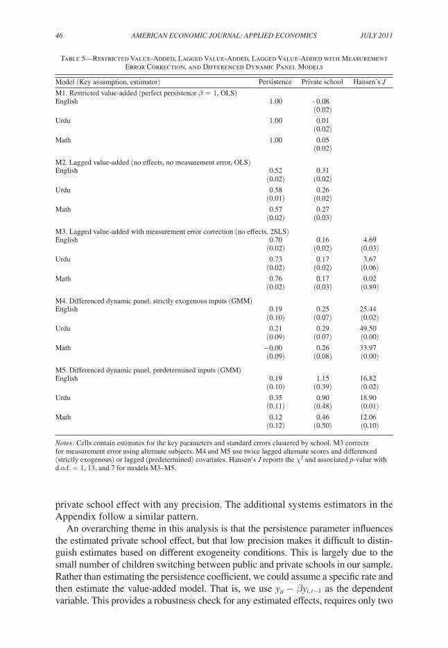
46 AMErIcAn EcOnOMIc JOUrnAL: APPLIEd EcOnOMIcs JULy 2011
private school effect with any precision. The additional systems estimators in the Appendix follow a similar pattern.
An overarching theme in this analysis is that the persistence parameter influences the estimated private school effect, but that low precision makes it difficult to distin-guish estimates based on different exogeneity conditions. This is largely due to the small number of children switching between public and private schools in our sample. Rather than estimating the persistence coefficient, we could assume a specific rate and then estimate the value-added model. That is, we use y it − β y i, t−1 as the dependent variable. This provides a robustness check for any estimated effects, requires only two
Table 5—Restricted Value-Added, Lagged Value-Added, Lagged Value-Added with Measurement Error Correction, and Differenced Dynamic Panel Models
Model (Key assumption, estimator) Persistence Private school Hansen’s J
M1. Restricted value-added (perfect persistence β = 1, OLS)English 1.00 −0.08
(0.02)Urdu 1.00 0.01
(0.02)Math 1.00 0.05
(0.02)
M2. Lagged value-added (no effects, no measurement error, OLS)English 0.52 0.31
(0.02) (0.02)Urdu 0.58 0.26
(0.01) (0.02)Math 0.57 0.27
(0.02) (0.03)
M3. Lagged value-added with measurement error correction (no effects, 2SLS)English 0.70 0.16 4.69
(0.02) (0.02) (0.03)Urdu 0.73 0.17 3.67
(0.02) (0.02) (0.06)Math 0.76 0.17 0.02
(0.02) (0.03) (0.89)
M4. Differenced dynamic panel, strictly exogenous inputs (GMM)English 0.19 0.25 25.44
(0.10) (0.07) (0.02)Urdu 0.21 0.29 49.50
(0.09) (0.07) (0.00)Math −0.00 0.26 33.97
(0.09) (0.08) (0.00)
M5. Differenced dynamic panel, predetermined inputs (GMM)English 0.19 1.15 16.82
(0.10) (0.39) (0.02)Urdu 0.35 0.90 18.90
(0.11) (0.48) (0.01)Math 0.12 0.46 12.06
(0.12) (0.50) (0.10)
notes: Cells contain estimates for the key parameters and standard errors clustered by school. M3 correctsfor measurement error using alternate subjects. M4 and M5 use twice lagged alternate scores and differenced (strictly exogenous) or lagged (predetermined) covariates. Hansen’s J reports the χ2 and associated p-value with d.o.f. = 1, 13, and 7 for models M3–M5.

VOL. 3 nO. 3 47AndrABI ET AL.: dO VALUE-AddEd EsTIMATEs Add VALUE?
years of data, and eliminates the need for complicated measurement error corrections. (It assumes, however, that inputs are uncorrelated with the omitted learning hetero-geneity.) Moving from the restricted value-added model (β = 1) to the pooled cross-section model (β = 0) increases the estimated effect from negative or insignificant to large and significant. For most of the range of the persistence parameter, the private school effect is positive and significant, but pinning down the precise yearly contribu-tion of private schooling depends on our assumptions about how children learn.
A couple of natural questions are how these estimates compare to the private-public differences reported in the cross-section and why the trajectories in Figure 1 are parallel even though the private school effect is positive. Controlling for observ-ables suggests that, after three years, children in private schools are 0.9 (English), 0.5 (Urdu), and 0.45 (mathematics) standard deviations ahead of their public school counterparts. If persistence is 0.4 and the yearly private school effect is 0.3, chil-dren’s trajectories will become parallel when that achievement gap reaches 0.5 (= 0.3/(1 − 0.4)). This is roughly the gap we find in Urdu and mathematics. Any small disagreement, including the larger gap in English, may be attributable to base-line selection effects. Thus, our results provide a partial resolution of the large base-line gap in achievement, the parallel achievement trajectories in public and private schools, and the significant and ongoing positive private school effect.
regression diagnostics.—For many of the GMM estimates, Hansen’s J test rejects the overidentifying restrictions implied by the model. This is troubling but not entirely unexpected. Different instruments may be identifying different local average treatment effects in the education context. For example, the portion of third grade achievement that remains correlated with fourth grade achievement may decay at a different rate than what was learned most recently. This is particularly true in an optimizing model of skill formation where parents smooth away shocks to achievement. In such a model, unexpected shocks to achievement, beyond measure-ment error, would fade more quickly than expected gains. Instrumenting using con-temporaneous alternate subject scores will therefore more likely identify different parameters than instrumenting using previous year scores. Likewise, instrumenting using alternate lags, differenced achievement and/or inputs may also identify dif-ferent effects. One result of note is that dropping the overidentifying inputs typically raises the persistence coefficient slightly, to roughly 0.25 for math. This type of het-erogeneity is important and suggests that a richer model than a constant coefficient lagged value-added may be warranted.
C. robustness checks
If our estimates are interpreted as forgetting, children lose over half of their achievement in a single year. For some subjects, such as mathematics, this frac-tion may be even larger. One potential explanation for low persistence is attrition. Roughly one-third of our original tested sample cannot be included in our estimates due to missing intermediate or final test scores. Lower scoring students are more likely to attrit, and it is possible that these students also experience little growth in learning from year to year. If so, these students will display high persistence in test

48 AMErIcAn EcOnOMIc JOUrnAL: APPLIEd EcOnOMIcs JULy 2011
scores year to year and excluding them from the analysis will bias our estimates downward. We find little evidence that this is a significant source of bias. Using the sample of children that attrit in fifth grade yields similar or even slightly lower esti-mates for persistence and more sophisticated corrections for attritition using inverse probability weighting, as in John M. Abowd, Bruno Crepon, and Francis Kramarz (2001), do not change our estimates significantly (see Appendix B).9
Furthermore, while these estimates may appear implausibly high, they match recent work on fade-out in value-added models, as well as the rapid fade-out observed in most educational interventions. Table 6 summarizes ten randomized (or quasi-randomized) interventions that followed children after the program ended. This follow-up enables estimation of both immediate and extended treatment effects. For the interventions summarized, the extended treatment effect represents test scores roughly one year after the particular program ended. For a number of the interventions, the persistence coefficient is less than 0.10. In two interventions—learning incentives and grade retention—the coefficient is between 0.6 and 0.7. However, this higher level of persistence may in part be explained by the specific nature of these interventions.10 Perhaps most interestingly, Duflo, Pascaline Dupas, and Kremer (2010) report results from an experiment providing both additional con-tract teachers and tracking students. While the impact of contract teachers fades out, consistent with our results, the effect of the tracking treatment increases over time in the same experimental context, even though children returned to the same classes after the experiment concluded. Although the link between fade-out in experimental studies and the persistence parameter is not always exact, the evidence from several randomized studies suggests that current learning does not always carry over to future learning without loss, and, in fact, these losses may be substantial for most treatments. Evaluating long-run outcomes appears critical to understanding the ulti-mate efficacy of educational interventions.
IV. Conclusion
In the absence of randomized studies, the value-added approach to estimating education production functions has gained momentum as a valid methodology for removing unobserved individual heterogeneity in assessing the contribution of specific programs or in understanding the contribution of school-level fac-tors for learning (e.g., Boardman and Murnane 1979; Hanushek 1979; Todd and Wolpin 2003; Hanushek 2003; Harold C. Doran and Lance T. Izumi 2004; Daniel F. McCaffrey et al. 2004; Gordon, Kane, and Staiger 2006). In such models, assumptions about learning persistence and unobserved heterogeneity play cen-tral roles. Our results reject both the assumption of perfect persistence required for
9 Two further robustness checks are reported in Andrabi et al. (2009). Our low-persistence estimates are consis-tent with the expected bias under OLS given plausible data generating processes and with an assumption of equal selection on observed and unobserved variables.
10 In the case of grade retention, there is no real “post-treatment” period since children always remain one grade behind after being retained. If one views grade retention as an ongoing multi-period treatment, then lasting effects can be consistent with low persistence. In the case of learning incentives, Kremer, Edward Miguel, and Rebecca Thornton (2004) argue that student incentives increased effort (not just achievement) even after the program ended, leading to ongoing learning.

VOL. 3 nO. 3 49AndrABI ET AL.: dO VALUE-AddEd EsTIMATEs Add VALUE?
the restricted value-added model and of no-learning heterogeneity required for the lagged value-added model. Our estimates of low persistence are consistent with recent work on teacher effects and with experimental evidence of program fade-out in developing and developed countries. These results illustrate the danger of incorrectly modeling or estimating education production functions; the restricted value-added model is fundamentally misspecified and can even yield wrong-signed estimates of a program’s impact. Underscoring the potential of afford-able, mainstream private schools in developing countries, we find that Pakistan’s private schools contribute roughly 0.25 standard deviations more to achievement each year than government schools, an effect greater than the average yearly gain between third and fourth grade.
However, the economic interpretation of low persistence still remains an area open to enquiry. Our context and test largely rule out mechanical explanations of low persistence such as psychometric bounding effects, cheating, or changing con-tent. In a preliminary exploration, we also found little evidence that low persistence results from substitution by parents and teachers (Andrabi et al. 2009). Simple for-getting, consistent with a large body of memory research in psychology, appears to be a likely explanation and hence a core component of education production functions. But more research is needed to provide direct evidence for it, and to understand whether the inability to perform on a test implies that the underlying knowledge has been truly lost.
Our results also suggest that short evaluations, even when experimental, may yield little information about the cost-effectiveness of a program. Using the one or two year increase from a program gives an upper-bound on the longer term achievement gains. As our estimates suggest, and Table 6 confirms, we should
Table 6—Experimental Estimates of Program Fade-Out
Program Subject
Immediate treatment
effect
Extended treatment
effect
Implied persistencecoefficient Source
Balsakhi program Math 0.348 0.030 0.086 Banerjee et al. (2007)Verbal 0.227 0.014 0.062
CAL program Math 0.366 0.097 0.265 Banerjee et al. (2007)Verbal 0.014 −0.078 ∼0.0
Learning incentives Multi-subject 0.23 0.16 0.70 Kremer, Miguel, and Thornton (2004)
Teacher incentives Multi-subject 0.139 −0.008 ∼0.0 Glewwe et al. (2003)Tracked classes Multi-subject 0.138 0.163 1.2 Duflo, Dupas, and
Kremer (2010)Contract teachers Multi-subject 0.181 0.094 0.52 Duflo, Dupas, and
Kremer (2010)STAR class size experiment
Stanford-9 and CTBS
∼5 percentile points
∼2 percentile points
∼0.25 to 0.5 Krueger and Whitmore (2001)
Summer school and grade retention
Math Reading
0.1360.104
0.0950.062
0.700.60
Jacob and Lefgren (2004)
notes: Extended treatment effect is achievement approximately one year after the treatment ended. Unless other-wise noted, effects are expressed in standard deviations. Results for Kremer (2003) are averaged across boys and girls. Estimated effects for Jacob and Lefgren (2004) are taken for the third grade sample.

50 AMErIcAn EcOnOMIc JOUrnAL: APPLIEd EcOnOMIcs JULy 2011
expect program impacts to fade quickly. Calculating the internal rate of return by citing research linking test scores to earnings of young adults is therefore a doubtful proposition. The techniques described here, with three periods of data, can theoretically obtain a lower bound on cost-effectiveness by assuming expo-nential fade-out. At the same time, the causes of fade-out are equally important; if parents no longer need to hire tutors or buy textbooks (the substitution inter-pretation of imperfect persistence), a program may be cost-effective even if test scores fade out.
Moving forward, empirical estimates of education production functions may benefit from further unpacking persistence. Overall, the agenda pleads for a richer model of education and for empirical techniques for modeling the broader learning process, not simply to add nuance to our understanding of learning but to get the most basic parameters right.
Appendix: Additional Estimation Strategies
A. system GMM
One difficulty with the differences GMM approach (M4 and M5) is that time-invariant inputs drop out of the estimated equation and their effects are there-fore not identified. In our case, this means that the identification of the private school effect is based on the 5 percent of children who switch between public and private schools. This leads to large standard errors in Table 5. We address the limited time-series variation using the levels and differences GMM framework proposed by Arellano and Bover (1995) and extended by Richard Blundell and Bond (1998). Levels and differences GMM estimate a system of equations, one for the undifferenced levels equation (5) and another for the differenced equation (7). Further assumptions regarding the correlation between inputs and heteroge-neity (though not necessarily between heterogeneity and lagged achievement) yield additional instruments; Andrabi et al. (2009) provide a description of these estimators.
We consider three options. First, we examine predetermined inputs that have a constant correlation with the individual effects (M6), which implies that Δ x it are available as instruments in the levels equation (Arellano and Bover 1995). Second, we assume inputs are predetermined but are also uncorrelated with the omitted effects (M7), which allows using inputs x i t as instruments in the levels model (5). Finally, in some instances, it may be reasonable to assume that, while learning heterogeneity exists, it does not affect achievement gains. A talented child may be so far ahead that imperfect persistence cancels the benefit of faster learning. That is, individual heterogeneity may be uncorrelated with gains, y it * − y i, t−1 * , but not necessarily with learning, y it * − β y i, t−1 * . This situation arises when the initial conditions have reached a convergent level with respect to the fixed effect such that
(9) y i1 * = η i _ 1 − β + d i ,

VOL. 3 nO. 3 51AndrABI ET AL.: dO VALUE-AddEd EsTIMATEs Add VALUE?
where t = 1 is the first observed period and not the first period in the learning life-cycle, see Blundell and Bond (1998) for a detailed discussion.
While this assumption seems too strong in the context of education, we discuss it because the dynamic panel literature has documented large downward biases of other estimators when the instruments are weak (e.g., Blundell and Bond 1998). The conditional mean stationarity assumption provides an additional T − 2 non-redundant moment conditions that can augment the system GMM estimators and ensures strong instruments in the levels equation to identify β. Thus, if we prefer simplicity over efficiency, we can estimate the model using levels GMM or 2SLS and avoid the need to use a system estimator. In this simpler approach, we instru-ment the undifferenced value-added model (5) using lagged changes in achieve-ment, Δ y i *t−1 , and either changes in inputs, Δ x i t , or inputs directly, x i t , depending on whether inputs are constantly correlated (M8) or are uncorrelated with the indi-vidual effect (M9).
Table B1 reports the persistence and private school effect for these additional estimators. Most estimators have higher, but still lower the lagged model, persis-tence estimates. With the addition of a conditional mean stationarity assumption, we can more precisely estimate the persistence coefficient. In this model, we only use moments in levels to illustrate a dynamic panel estimator that improves over the lagged value-added model estimated by OLS but doesn’t require estimating a system of equations. The persistence coefficient rises substantially to between 0.39 and 0.56. This upward movement is consistent with a violation of the station-arity assumption (the fixed-effect still contributes to achievement growth) but an overall reduction in the omitted heterogeneity bias. Across the various dynamic panel models and subjects, estimates of the persistence parameter vary from 0.2 to 0.55. However, the highest dynamic panel estimates come from assuming con-ditional mean stationarity, which is likely too strong an assumption in the context of learning.
Adding a levels equation and using the assumption that inputs are constantly correlated or uncorrelated with the omitted effects reduces the standard errors for the private school coefficient while maintaining the assumption that inputs are predetermined but not strictly exogenous. Under the scenario that private school enrollment is constantly correlated with the omitted effect (M6), the private school coefficient is large, 0.19 to 0.32 standard deviations (depending on the subject), and statistically significant. This estimate allows for past achievement shocks to affect enrollment decisions but assumes that switching school type is uncorrelated with unobserved student heterogeneity. Within the systems context, this is our preferred estimate.
B. Attrition corrected Estimators
To fully correct for attrition in a moment-based model such as ours, Abowd, Crepon, and Kramarz (2001) propose weighting by the estimated inverse proba-bility that each observation remains in the sample. Analogous to propensity score weighting in the program evaluation literature, inverse probability weighting elimi-nates potential attrition bias if attrition is based on observables. To evaluate potential

52 AMErIcAn EcOnOMIc JOUrnAL: APPLIEd EcOnOMIcs JULy 2011
attrition bias, we estimate the probability of attrition using all past test scores and child characteristics and report our weighted results for two models in Table B2. Reassuringly, these corrections for attrition make little difference. Both the private school coefficient and the persistence coefficient change only slightly compared to Tables 5 and B1, and the direction of change differs across models and subjects. The likely explanation for why corrections for attrition do not affect our estimates is that the bulk of children who are not tested in any given year are not dropouts but children absent on the day of the test, which may be a largely random process. Indeed, simple OLS estimates of persistence based on the subsample of children who report only 2 years of test-scores are within 0.05 standard deviations of esti-mates based on children who were present for all 3 tests, and the difference is sta-tistically insignificant.
Table B1—System and Levels Only Dynamic Panel Models
English
Model (Key assumption, estimator) Persistence Private school Hansen’s J
Levels and difference sGMMM6. Predetermined inputs, constantly correlated effectsEnglish 0.36 0.21 45.50
(0.07) (0.06) 0.00
Urdu 0.26 0.22 66.58(0.08) (0.06) (0.00)
Math 0.12 0.19 57.63(0.10) (0.08) (0.00)
M7. Predetermined inputs, uncorrelated effectsEnglish 0.53 0.32 79.08
(0.05) (0.04) 0.00
Urdu 0.51 0.30 81.89(0.06) (0.04) (0.00)
Math 0.51 0.30 82.19(0.08) (0.05) (0.00)
Levels only GMMM8. Predetermined inputs, constantly correlated effects, conditional stationarityEnglish 0.40 0.29 24.74
(0.05) (0.07) (0.02)Urdu 0.55 0.31 13.49
(0.05) (0.07) (0.33)Math 0.51 0.30 29.45
(0.06) (0.07) (0.00)M9. Predetermined inputs, uncorrelated effects, conditional stationarityEnglish 0.39 0.24 23.43
(0.05) (0.04) (0.02)Urdu 0.56 0.27 13.30
(0.05) (0.03) (0.27)Math 0.53 0.27 28.36
(0.06) (0.04) (0.00)
notes: Cells contain estimates for the key parameters and standard errors clustered by school. M6 and M7 are system estimators, including both a difference and levels equation with differenced (M6) or undifferenced (M7) covariates as additional instruments in the levels equation. M8 and M9 use only the levels equation for simplicity and included differenced scores as an additional instrument. Hansen’s J reports the χ2 and associated p-value with df=23, 29, 12, and 11.

VOL. 3 nO. 3 53AndrABI ET AL.: dO VALUE-AddEd EsTIMATEs Add VALUE?
REFERENCES
Abowd, John M., Bruno Crepon, and Francis Kramarz. 2001. “Moment Estimation with Attrition: An Application to Economic Models.” Journal of the American statistical Association, 96(456): 1223–31.
Alderman, Harold, Jooseop Kim, and Peter F. Orazem. 2003. “Design, Evaluation, and Sustainability of Private Schools for the Poor: The Pakistan Urban and Rural Fellowship School Experiments.” Economics of Education review, 22(3): 265–74.
Alderman, Harold, Peter F. Orazem, and Elizabeth M. Paterno. 2001. “School Quality, School Cost, and the Public/Private School Choices of Low-Income Households in Pakistan.” Journal of Human resources, 36(2): 304–26.
Andrabi, Tahir, Jishnu Das, and Asim Ijaz Khwaja. 2006. “A Dime a Day: The Possibilities and Limits of Private Schooling in Pakistan.” World Bank Policy Research Working Paper 4066.
Andrabi, Tahir, Jishnu Das, and Asim Ijaz Khwaja. 2008. “A Dime a Day: The Possibilities and Limits of Private Schooling in Pakistan.” comparative Education review, 52(3): 329–55.
Andrabi, Tahir, Jishnu Das, Asim Ijaz Khwaja, and Tristan Zajonc. 2009. “Do Value-Added Estimates Add Value: Accounting for Learning Dynamics?” Harvard University Kennedy School of Govern-ment Working Paper.
Andrabi, Tahir, Jishnu Das, Asim Ijaz Khwaja, and Tristan Zajonc. 2011. “Do Value-Added Estimates Add value? Accounting for Learning Dynamics: Dataset.” American Economic Journal: Applied Economics http://www.aeaweb.org/articles.php?doi=10.1257/app.3.3.29.
Angrist, Joshua, Eric Bettinger, Erik Bloom, Elizabeth King, and Michael Kremer. 2002. “Vouchers for Private Schooling in Colombia: Evidence from a Randomized Natural Experiment.” American Economic review, 92(5): 1535–58.
Arellano, Manuel. 2003. Panel data Econometrics. New York: Oxford University Press.Arellano, Manuel, and Stephen Bond. 1991. “Some Tests of Specification for Panel Data: Monte Carlo
Evidence and an Application to Employment Equations.” review of Economic studies, 58(2): 277–97.Arellano, Manuel, and Olympia Bover. 1995. “Another Look at the Instrumental Variable Estimation
of Error-Components Models.” Journal of Econometrics, 68(1): 29–51.Arellano, Manuel, and Bo Honoré. 2001. “Panel Data Models: Some Recent Developments.” In Hand-
book of Econometrics. Vol. 5, ed. James J. Heckman and Edward Leamer, 3229–96. Amsterdam: Elsevier Science, North-Holland.
Banerjee, Abhijit V., Shawn Cole, Esther Duflo, and Leigh Linden. 2007. “Remedying Education: Evidence from Two Randomized Experiments in India.” Quarterly Journal of Economics, 122(3): 1235–64.
Blundell, Richard, and Stephen Bond. 1998. “Initial Conditions and Moment Restrictions in Dynamic Panel Data Models.” Journal of Econometrics, 87(1): 115–43.
Boardman, Anthony E., and Richard J. Murnane. 1979. “Using Panel Data to Improve Estimates of the Determinants of Educational Achievement.” sociology of Education, 52(2): 113–21.
Table B2—Correcting for Potential Attrition Bias using Inverse Probability Weighting
Strategy English Urdu Math
M2. no effects, no measurement error (OLs)Private school 0.28
(0.03)0.22
(0.03)0.22
(0.03)Persistence 0.55
(0.02)0.59
(0.02)0.65
(0.02)
M8. Predetermined inputs, constantly correlated effects, conditional stationarityPrivate school 0.25
(0.07)0.28
(0.08)0.30
(0.09)Persistence 0.40
(0.05)0.55
(0.05)0.50
(0.06)
notes: Cells give model coefficients and parentheses give standard errors. Models mirror Table 4, 5, and 6 but weight the sample using the estimated inverse probability of an observation being observed. The probability of attri-tion is estimated from two logit regressions for fourth and fifth grade including all previous data as controls and vil-lage fixed effects. See Abowd, Crepon, and Kramarz (2001) for details.

54 AMErIcAn EcOnOMIc JOUrnAL: APPLIEd EcOnOMIcs JULy 2011
Chay, Kenneth Y., Patrick J. McEwan, and Miguel Urquiola. 2005. “The Central Role of Noise in Evaluating Interventions that Use Test Scores to Rank Schools.” American Economic review, 95(4): 1237–58.
Cunha, Flavio, and James J. Heckman. 2008. “Formulating, Identifying and Estimating the Technol-ogy of Cognitive and Noncognitive Skill Formation.” Journal of Human resources, 43(4): 738–82.
Cunha, Flavio, James J. Heckman, and Susanne M. Schennach. 2010. “Estimating the Technology of Cognitive and Noncognitive Skill Formation.” Econometrica, 78(3): 883–931.
Currie, Janet, and Duncan Thomas. 1995. “Does Head Start Make a Difference?” American Economic review, 85(3): 341–64.
Deming, David. 2009. “Early Childhood Intervention and Life-Cycle Skill Development: Evidence from Head Start.” American Economic Journal: Applied Economics, 1(3): 111–34.
Doran, Harold C., and Lance T. Izumi. 2004. “Putting Education to the Test: A Value-Added Model for California.” San Francisco: Pacific Research Institute.
Duflo, Esther, Pascaline Dupas, and Michael Kremer. 2010. “Peer Effects, Teacher Incentives, and the Impact of Tracking: Evidence from a Randomized Evaluation in Kenya.” National Bureau Eco-nomic Research Working Paper 14475.
Glewwe, Paul, Nauman Ilias, and Michael Kremer. 2010. “Teacher Incentives.” American Economic Journal: Applied Economics, 2(3): 205–27.
Gordon, Robert, Thomas J. Kane, and Douglas O. Staiger. 2006. “Identifying Effective Teachers Using Performance on the Job.” Hamilton Project Discussion Paper 2006-01.
Hanushek, Eric A. 1979. “Conceptual and Empirical Issues in the Estimation of Educational Produc-tion Functions.” Journal of Human resources, 14(3): 351–88.
Hanushek, Eric A. 2003. “The Failure of Input-Based Schooling Policies.” Economic Journal, 113(485): F64–98.
Harris, Douglas, and Timothy R. Sass. 2006. “Value-Added Models and the Measurement of Teacher Quality.” http://myweb.fsu.edu/tsass/Papers/IES%20Harris%20Sass%20EPF%20Value-added%2014.pdf.
Jacob, Brian A., Lars Lefgren, and David P. Sims. 2010. “The Persistence of Teacher-Induced Learn-ing.” Journal of Human resources, 45(4): 915–43.
Jimenez, Emmanuel, Marlaine E. Lockheed, and Vicente Paqueo. 1991. “The Relative Efficiency of Pri-vate and Public Schools in Developing Countries.” World Bank research Observer, 6(2): 205–18.
Kane, Thomas J., and Douglas O. Staiger. 2002. “The Promise and Pitfalls of Using Imprecise School Accountability Measures.” Journal of Economic Perspectives, 16(4): 91–114.
Kane, Thomas J., and Douglas O. Staiger. 2008. “Estimating Teacher Impacts on Student Achieve-ment: An Experimental Evaluation.” National Bureau of Economic Research Working Paper 14607.
Kremer, Michael, Edward Miguel, and Rebecca Thornton. 2004. “Incentives to Learn.” National Bureau of Economic Research Working Paper 10971.
Krueger, Alan B. 2003. “Economic Considerations and Class Size.” Economic Journal, 113(485): F34–63.Krueger, Alan B., and Diane M. Whitmore. 2001. “The Effect of Attending a Small Class in the Early
Grades on College-Test Taking and Middle School Test Results: Evidence from Project STAR.” Economic Journal, 111(468): 1–28.
Ladd, Helen F., and Randall P. Walsh. 2002. “Implementing Value-Added Measures of School Effec-tiveness: Getting the Incentives Right.” Economics of Education review, 21(1): 1–17.
Lord, Frederic M. 1967. “A Paradox in the Interpretation of Group Comparisons.” Psychological Bul-letin, 68(5): 304–05.
McCaffrey, Daniel F., J. R. Lockwood, Daniel M. Koretz, and Laura S. Hamilton. 2004. Evaluating Value-Added Models for Teacher Accountability. Santa Monica: Rand Corporation.
Murnane, Richard J., John B. Willett, and Frank Levy. 1995. “The Growing Importance of Cognitive Skills in Wage Determination.” review of Economics and statistics, 77(2): 251–66.
Neal, Derek A., and William R. Johnson. 1996. “The Role of Premarket Factors in Black-White Wage Differences.” Journal of Political Economy, 104(5): 869–95.
Rothstein, Jesse. 2010. “Teacher Quality in Educational Production: Tracking, Decay, and Student Achievement.” Quarterly Journal of Economics, 125(1): 175–214.
Schweinhart, Lawrence J., Jeanne Montie, Zongping Xiang, William S. Barnett, Clive R. Belfield, and Milagros Nores. 2005. Lifetime Effects: The High/scope Perry Preschool study Through Age 40. Ypsilanti, MI: High/Scope Press.
Todd, Petra E., and Kenneth I. Wolpin. 2003. “On the Specification and Estimation of the Production Function for Cognitive Achievement.” Economic Journal, 113(485): F3–33.
Tooley, James, and Pauline Dixon. 2003. Private schools for the Poor: A case study from India. Read-ing, UK: Centre for British Teachers.

This article has been cited by:
1. Weili Ding, Steven F. Lehrer. 2014. Understanding the role of time-varying unobserved abilityheterogeneity in education production. Economics of Education Review 40, 55-75. [CrossRef]
2. Scott A. Imberman, Adriana D. Kugler. 2014. The Effect of Providing Breakfast in Class onStudent Performance. Journal of Policy Analysis and Management n/a-n/a. [CrossRef]
3. Tim R. Sass, Anastasia Semykina, Douglas N. Harris. 2014. Value-added models and themeasurement of teacher productivity. Economics of Education Review 38, 9-23. [CrossRef]
4. Elizabeth Dhuey. 2013. Middle school or junior high? How grade-level configurations affectacademic achievement. Canadian Journal of Economics/Revue canadienne d'économique 46:2,469-496. [CrossRef]
5. Tahir Andrabi, Jishnu Das, Asim Ijaz Khwaja. 2013. Students today, teachers tomorrow:Identifying constraints on the provision of education. Journal of Public Economics 100, 1-14.[CrossRef]
6. Jishnu Das,, Stefan Dercon,, James Habyarimana,, Pramila Krishnan,, Karthik Muralidharan,,Venkatesh Sundararaman. 2013. School Inputs, Household Substitution, and Test Scores.American Economic Journal: Applied Economics 5:2, 29-57. [Abstract] [View PDF article] [PDFwith links]
7. Subha Mani, John Hoddinott, John Strauss. 2012. Long-term impact of investments in earlyschooling — Empirical evidence from rural Ethiopia. Journal of Development Economics 99:2,292-299. [CrossRef]
8. David McKenzie. 2012. Beyond baseline and follow-up: The case for more T in experiments.Journal of Development Economics 99:2, 210-221. [CrossRef]
9. Jenny C. Aker,, Christopher Ksoll,, Travis J. Lybbert. 2012. Can Mobile Phones ImproveLearning? Evidence from a Field Experiment in Niger. American Economic Journal: AppliedEconomics 4:4, 94-120. [Abstract] [View PDF article] [PDF with links]