Do Hedge Funds Exploit Rare Disaster Concerns?�

George P. Gaoy, Pengjie Gaoz, and Zhaogang Songx

First Draft: July 2012This Draft: July 2016

Abstract

We �nd hedge funds that have higher return covariation with a disaster concern index, wihch

we develop through out-of-the-money puts on various economic sector indices, earn signi�cantly

higher returns in the cross section. We provide substantial evidence that these funds have better

skills in exploiting the market�s ex ante rare disaster concerns (SED), which may not realize as

disaster shocks ex post. In particular, high-SED funds on average outperform low-SED funds

by 0:96% per month, but have less exposure to disaster risk. They continue to deliver superior

future performance when SED is estimated using the disaster concern index purged of disaster

risk premium, and have leverage-managing and extreme-market-timing abilities. We also provide

strong evidence against alternative interpretations.

Keywords: Rare disaster concern; hedge fund; skill

JEL classi�cations: G11; G12; G23

�We would like to thank Warren Bailey, Sanjeev Bhojraj, Craig Burnside, Martijn Cremers, Zhi Da, ChristianDorion, Itamar Drechsler, Ravi Jagannathan, Bob Jarrow, Alexandre Jeanneret, Andrew Karolyi, Soohun Kim,Veronika Krepely, Tim Loughran, Bill McDonald, Roni Michaely, Pam Moulton, Narayan Naik, David Ng, MaureenO�Hara, Sugata Ray, Gideon Saar, Paul Schultz, David Schumacher, Berk Sensory, Mila Getmansky Sherman, LauraStarks (the editor), Shu Yan, Jianfeng Yu, Lu Zheng, Hao Zhou, and two anonymous referees for their helpfuldiscussions and comments, as well as seminar participants at the City University of Hong Kong, Cornell University,HEC Montreal, University of Notre Dame, the 2013 China International Conference in Finance, the 2013 EFA AnnualMeeting, the 2013 FMA Annual Meetings, the 2014 MFA Annual Meetings, the 2015 AFA Annual Meetings, the 3rdLuxembourg Asset Management Summit, the 6th Paris Hedge Fund Research Conference, Texas A&M University, andUniversity of Hawaii. We are especially grateful to Zheng Sun for help on clustering analysis; Kuntara Pukthuanthongfor data on benchmark factors; and Sang Seo and Jessica Wachter for data on model-implied option prices. Financialsupport from the Q-group is gratefully acknowledged. The RIX index and its components are available from authors�websites for academic use. The analysis and conclusions set forth are those of the authors and do not indicateconcurrence by the Board of Governors of the Federal Reserve System.

ySamuel Curtis Johnson Graduate School of Management, Cornell University. Email: pg297@cornell.edu; Tel:(607) 255�8729

zFinance Department, Mendoza College of Business, University of Notre Dame. E-mail: pgao@nd.edu; Tel: (574)631-8048.

xCarey Business School, Johns Hopkins University. E-mail: zsong8@jhu.edu. Tel: (410)-234-9392

2

1 Introduction

Prior research on hedge fund performance and disaster risk focuses on the covariance between fund

returns and ex post realized disaster shocks. In the time series, a number of hedge fund investment

styles, characterized as de facto sellers of put options, incur substantial losses when the market

goes south (Mitchell and Pulvino (2001) and Agarwal and Naik (2004)). In the cross section,

individual hedge funds have heterogeneous disaster risk exposure, and funds with larger exposure

to disaster risk usually earn higher returns during normal times, followed by losses during stressful

times (Agarwal, Bakshi, and Huij (2010); Jiang and Kelly (2012)). At its face value, the existing

evidence suggests that hedge funds are much like conventional assets in an economy with disaster

risk: they earn higher returns simply by being more exposed to disaster risk.

We provide novel evidence that some hedge fund managers with skills in exploiting ex ante

market disaster concerns, which may not be realized as ex post disaster shocks, deliver superior

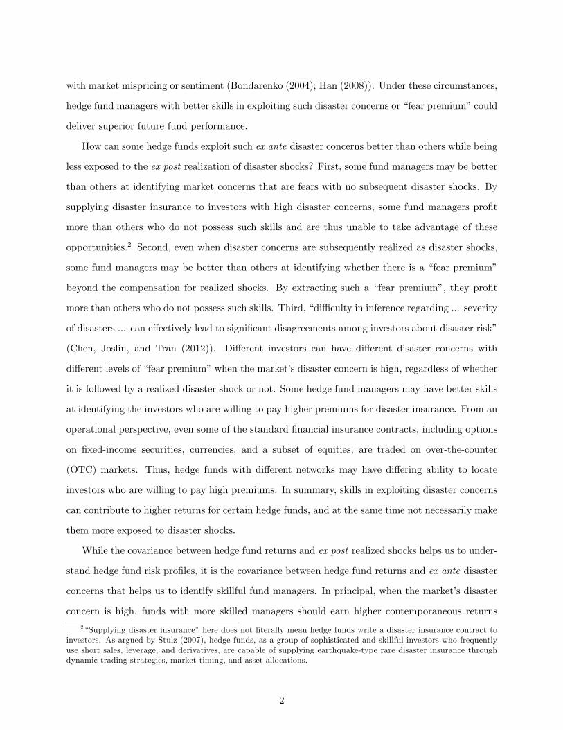
future fund performance while being less exposed to disaster risk. Our basic idea is illustrated in

Figure 1, which plots the monthly time-series of a rare disaster concern index (RIX) we construct

using out-of-the-money put options on various economic sector indices. The index value at time t

is essentially equal to the price of insurance against extreme downside movements of the �nancial

market from time t to (t+ �) in the future (see Section 2 for details). The graph shows the following

salient feature of the market�s disaster concerns.

When market shocks occur at time t, concerns for future disasters between t and (t+�) increases

substantially. Most importantly, the magnitude of such increased concerns at time t seems to be

enormous relative to subsequently realized losses, if any, between t and (t + �).1 This startling

di¤erence between the ex ante disaster concerns and the ex post realized shocks suggests that

investors may be paying a �fear premium�beyond the compensation for the disaster risk. In fact,

Bollerslev and Todorov (2011) suggest that the fear premium is a critical component of market

returns. Such a fear premium can be consistent with the behavior of agents with non-expected

utility or constrained agents who face market frictions and are averse to tail events (Liu, Pan, and

Wang (2005); Bates (2008); Caballero and Krishnamurthy (2008); Barberis (2013)), or consistent

1Another feature of disaster concerns is that the index spikes not only when disaster shocks hit the market suchas the LTCM collapse, the crash of Nasdaq, and the recent �nancial crisis, but also during bull markets such as thepeak of Nasdaq and the market rally in October 2011.

1

with market mispricing or sentiment (Bondarenko (2004); Han (2008)). Under these circumstances,

hedge fund managers with better skills in exploiting such disaster concerns or �fear premium�could

deliver superior future fund performance.

How can some hedge funds exploit such ex ante disaster concerns better than others while being

less exposed to the ex post realization of disaster shocks? First, some fund managers may be better

than others at identifying market concerns that are fears with no subsequent disaster shocks. By

supplying disaster insurance to investors with high disaster concerns, some fund managers pro�t

more than others who do not possess such skills and are thus unable to take advantage of these

opportunities.2 Second, even when disaster concerns are subsequently realized as disaster shocks,

some fund managers may be better than others at identifying whether there is a �fear premium�

beyond the compensation for realized shocks. By extracting such a �fear premium�, they pro�t

more than others who do not possess such skills. Third, �di¢ culty in inference regarding ... severity

of disasters ... can e¤ectively lead to signi�cant disagreements among investors about disaster risk�

(Chen, Joslin, and Tran (2012)). Di¤erent investors can have di¤erent disaster concerns with

di¤erent levels of �fear premium�when the market�s disaster concern is high, regardless of whether

it is followed by a realized disaster shock or not. Some hedge fund managers may have better skills

at identifying the investors who are willing to pay higher premiums for disaster insurance. From an

operational perspective, even some of the standard �nancial insurance contracts, including options

on �xed-income securities, currencies, and a subset of equities, are traded on over-the-counter

(OTC) markets. Thus, hedge funds with di¤erent networks may have di¤ering ability to locate

investors who are willing to pay high premiums. In summary, skills in exploiting disaster concerns

can contribute to higher returns for certain hedge funds, and at the same time not necessarily make

them more exposed to disaster shocks.

While the covariance between hedge fund returns and ex post realized shocks helps us to under-

stand hedge fund risk pro�les, it is the covariance between hedge fund returns and ex ante disaster

concerns that helps us to identify skillful fund managers. In principal, when the market�s disaster

concern is high, funds with more skilled managers should earn higher contemporaneous returns

2�Supplying disaster insurance�here does not literally mean hedge funds write a disaster insurance contract toinvestors. As argued by Stulz (2007), hedge funds, as a group of sophisticated and skillful investors who frequentlyuse short sales, leverage, and derivatives, are capable of supplying earthquake-type rare disaster insurance throughdynamic trading strategies, market timing, and asset allocations.

2

than those with less skilled managers in supplying disaster insurance. Empirically, we measure

fund skills in exploiting rare disaster concerns (SED) using the covariation between fund returns

and the disaster concern index we construct.3 Consistent with our view that hedge funds exhibit

di¤erent levels of skills in exploiting disaster concerns, we document substantial heterogeneity of

SED across hedge funds as well as signi�cant persistence in SED.

Our main tests focus on the relation between the SED measure and future fund performance.

In our baseline results, funds in the highest SED decile on average outperform funds in the lowest

SED decile by 0:96% per month (Newey-West t-statistic of 2:8).4 Moreover, high-SED funds exhibit

signi�cant performance persistence. The return spread of the high-minus-low SED deciles ranges

from 0:84% per month (t-statistic of 2:6) for a three-month holding horizon, to 0:44% per month (t-

statistic of 1:9) for a 12-month holding horizon. We also show that the outperformance of high-SED

funds is pervasive across almost all hedge fund investment styles. These results are inconsistent

with the view that hedge funds earn higher returns on average simply by being more exposed to

disaster risk. If the SED measure, as the covariation between fund returns and the disaster concern

index, is interpreted as measuring disaster risk exposure, high-SED funds on average should earn

lower returns (rather than the higher returns we document) because they are good hedges against

disaster risk under this interpretation.

We further provide several pieces of collaborative evidence that SED captures the skills of

hedge funds in exploiting disaster concerns. First, if SED captures the skill rather than disaster

risk exposure of hedge funds, high-SED funds should be less exposed to disaster risk. We check

whether this is the case by computing loadings of SED fund deciles on a large set of macroeconomic

variables, liquidity factors, and option-based risk measures. We �nd strong evidence that high-SED

funds are actually less risky than low-SED funds, consistent with the interpretation that high-SED

funds posses better skills of exploiting disaster concerns. If our results are driven by some missing

risk factors, then these factors have to be nearly uncorrelated with all these known risk factors,

3 In the same vein, Sialm, Sun, and Zheng (2012) use fund-of-funds return loadings on some local/non-local factorsto measure the fund�s local bias, di¤erent from the conventional risk�� interpretation.

4We also perform time series analysis on dozens of hedge fund indices from Hedge Fund Research Inc. (HFRI).In estimating regressions of hedge fund index monthly excess returns on market excess return and the rare disasterconcern index (RIX), we �nd negative and statistically signi�cant RIX loadings for the majority of HFRI investmentstrategies. These results con�rm that the payo¤s of hedge fund strategies resemble the payo¤s of writing put options,and hence these strategies are sensitive to extreme downside market movements (Lo (2001); Goetzmann et al. (2002,2007); Agarwal and Naik (2004)).

3

which seems to be unlikely.

Second, given that our original RIX measure is the price of a disaster insurance contract that

contains compensations for both objective disaster shocks (rational disaster risk premiums) and

pure �concerns� (or �fears�) about disaster risk, we purge the disaster risk premium from RIX

based on the stochastic disaster risk model of Seo and Wachter (2014) and re-estimate funds�SED.

These SED estimates capture the fund skills in exploiting the pure �concerns�on disaster risk more

directly. We continue to observe high-SED funds strongly outperform low-SED funds with these

SED estimates, collaborating that high-SED funds earn higher returns because of their superior

skills in exploiting rare disaster concerns.

Third, we expect high-SED funds to have better abilities of managing leverage and timing

extreme market condition if SED captures skills because both are integrated parts of any disaster

episodes. We calculate the leverage implied by RIX and estimate each fund�s ability in managing

leverage. We �nd that high-SED funds do have leverage-managing ability: they reduce exposure

to market-wide leverage shocks when the market leverage condition worsens and the market is on

de-leverage. Moreover, we estimate each fund�s extreme-market-timing ability and �nd that high-

SED funds on average have strong bear-market-timing ability. Both results are consistent with

the interpretation of SED as measuring the fund skills, though we note that such evidence is only

suggestive because of the lack of fund-level data on portfolio holdings, investment positions, and

balance sheets.

We also provide strong empirical evidence against alternative interpretations. First, the higher

average returns high-SED funds earn over the full sample are just a result of better performance

during normal times and (hypothetically) worse performance during stressful times that are too

short in our sample period of 1996 - 2010. In other words, the high-SED funds are �lucky�in our

sample period. We perform a conditional test of SED-sorted fund portfolios during both normal

and stressful market times, but �nd that high-SED funds (based on either the original version of

RIX, or the version of RIX purged of the disaster risk premium) outperform low-SED funds even

more during stressful market times, including the severe 2008 �nancial crisis. Such evidence is

inconsistent with the �luck� interpretation and favors our skill-based explanation of hedge fund

performance.

Second, as the spikes in the RIX factor often occur when disaster shocks hit the market, it is

4

possible that some of our high-SED funds earn pro�ts by purchasing �rather than selling �disaster

insurance before the disaster shock: these funds realize large positive payo¤s when such disastrous

outcomes hit the market. Among the credit-style hedge fund sample, we identify a potential set

of such funds and �nd even stronger SED e¤ects on future fund performance after excluding them

from our portfolio analysis. Moreover, we explore a general identi�cation condition for the funds

purchasing disaster insurance: time t � 1 returns of these funds, who pay a cost to buy disaster

insurance before disastrous events at time t, should have signi�cant negative loadings on the RIX

at time t. Accordingly, we identify funds with skills of purchasing disaster insurance by regressing

the fund�s monthly excess return at t � 1 on the next-period RIX at t. We �nd that there is no

signi�cant return di¤erence between low- and high-exposure funds, contradicting the interpretation

of high-SED funds as purchasing disaster insurance. These results provide further support that

the skills of high-SED fund managers are to identify the existence and magnitude of the �fear

premium�and sell insurance contracts against future disaster events, rather than forecasting the

disaster event and buying disaster insurance beforehand.

Third, we investigate whether high-SED funds are those that exploit insurance associated with

intermediate rather than extreme tails of the market. The answer is unequivocally no. In particular,

we capture the intermediate tails of the market by the VIX given that it does not include extreme

volatility shocks induced by the extreme tail events (i.e., those captured by RIX). We �nd that

hedge fund portfolios formed on the covariation between fund excess returns and VIX (analogous

to SED) have no signi�cant return spreads. Moreover, sequential sorts show that SED, even in the

presence of potential fund skills in exploiting intermediate tails, well explains cross-sectional hedge

fund returns, but not vice versa. Collectively, these results suggest that fund skills in exploiting

disaster concerns rather than concerns on intermediate tail events explain cross-sectional hedge

fund performance.

Throughout the paper, we also compute risk-adjusted abnormal returns using the Fung and

Hsieh (2001) eight-factor model and the ten-factor model recently developed by Namvar, Phillips,

Pukthuanthong, and Rau (2014; NPPR (2014) hereafter). The return di¤erence between the high-

and low-SED funds remains highly signi�cant. Speci�cally, funds in the highest SED decile on

average outperform funds in the lowest SED decile by 1:27% and 0:80% per month with Newey-

West t-statistics of 3:8 and 2:8 relative to the Fung-Hsieh and NPPR models, respectively. In

5

addition, we conduct portfolio analysis and Fama-MacBeth (1973) regressions to account for hedge

fund characteristics and a number of risk factors developed in the hedge fund literature, including

market risk, downside market risk (Ang, Chen, and Xing (2006)), volatility risk (Ang et al. (2006)),

market liquidity risk (Pastor and Stambaugh (2003); Acharya and Pedersen (2005); Sadka (2006);

Hu, Pan, and Wang (2013)), funding liquidity risk (Brunnermeier and Pedersen (2009); Mitchell

and Pulvino (2012)), macroeconomic risk (Bali, Brown, and Caglayan (2011)), and hedge fund total

variance risk (Bali, Brown, and Caglayan (2012)). Our results remain similar in these extended

analyses.

In addition, we show that our results are robust to alternative measures of ex ante disaster

concerns such as the ones based on the S&P 500 index and long-maturity (90-day) options. Our

results also survive a battery of robustness checks including di¤erent choices of portfolio weight,

fund size, fund back�lling bias, fund delisting returns, fund December and non-December returns,

di¤erent benchmark models, and di¤erent hedge fund databases.

Our paper mainly contributes to the literature studying hedge fund skills and cross-sectional

fund performance.5 The SED measure is distinct from other fund skill variables in predicting

future fund performance, including the skill in hedging systematic risk (Titman and Tiu (2011)),

the skill in adopting innovative strategies (Sun, Wang, and Zheng (2012)), the skill in timing market

liquidity (Cao et al. (2013)), and the conditional performance measure of downside returns (Sun,

Wang, and Zheng (2013)).

The remainder of the paper is organized as follows. Section 2 describes the construction of our

rare disaster concern index. Section 3 presents the SED measure and its properties across the pool

of hedge funds. Section 4 reports our baseline results of cross-sectional fund performance based

on SED and provides collaborate evidence for the interpretation of SED as capturing fund skills

in exploiting disaster concerns. We provide strong evidence against alternative interpretations in

Section 5. Section 6 provides additional results and robustness checks, and Section 7 concludes.

The Appendix provides technical details, and a separate Internet Appendix provides open interest

statistics of index options and additional analyses of SED portfolios.

5Recent studies include Aragon (2007), Fung, Hsieh, Naik, and Ramadorai (2008), Liang and Park (2008),Agarwal, Daniel, and Naik (2009), Aggarwal and Jorion (2010), Li, Zhang, and Zhao (2011), Titman and Tiu (2011),Cao, Chen, Liang, and Lo (2013), and Sun, Wang and Zheng (2012, 2013), among others.

6

2 Quantify Rare Disaster Concerns

In this section, we develop a rare disaster concern index (RIX) to quantify the ex ante market

expectation about disaster events in the future, building on the model-free implied volatility mea-

sures of Carr and Madan (1998), Britten-Jones and Neuberger (2000), Carr and Wu (2009), and Du

and Kapadia (2012). In particular, the value of RIX depends on the price di¤erence between two

option-based replication portfolios of variance swap contracts. The �rst portfolio accounts for mild

market volatility shocks, and the second for extreme volatility shocks induced by market jumps

associated with rare event risk. By construction, the RIX is equal to the insurance price against

extreme downside market movements in the future. Over time, the RIX signals variations of ex

ante disaster concerns.

2.1 Construction of RIX

Consider an underlying asset whose time-t price is St. We assume for simplicity that the asset

does not pay dividends. An investor holding this security is concerned about its price �uctuations

over a time period [t; T ]. One way to protect herself against price changes is to buy a contract

that delivers payments equal to the extent of price variations over [t; T ], minus a prearranged price.

Such a contract is called a �variance� swap contract as the price variations are essentially about

the stochastic variance of the price process.6 The standard variance swap contract in practice pays

�lnSt+�St

�2+

�lnSt+2�St+�

�2+ � � �+

�ln

STST��

�2

minus the prearranged price VP. That is, the variance swap contract uses the sum of squared log

returns to measure price variations, which is a standard practice in the �nance literature (Singleton

(2006)).

In principle, replication portfolios consisting of out-of-the-money (OTM) options written on St

can be used to replicate the time-varying payo¤ associated with the variance swap contract and

hence to determine the price VP . We now introduce two replication portfolios and their implied

prices for the variance swap contract. The �rst, which underlies the construction of VIX by the

6The variance here refers to stochastic changes of the asset price, and hence is di¤erent from (and more generalthan) the second-order central moment of the asset return distribution.

7

CBOE, focuses on the limit of the discrete sum of squared log returns, determines VP as

IV � 2er�

�

�ZK>St

1

K2C(St;K;T )dK +

ZK<St

1

K2P (St;K;T )dK

�; (1)

where r is the constant risk-free rate, � � T � t is the time-to-maturity, and C(St;K;T ) and

P (St;K;T ) are prices of call and put options with strike K and maturity date T , respectively. As

observed from equation (1), this replication portfolio contains positions in OTM calls and puts with

a weight inversely proportional to their squared strikes. IV has been employed in the literature to

construct measures of variance risk premiums (Bollerslev, Tauchen, and Zhou (2009), Carr and Wu

(2009), and Drechsler and Yaron (2011)).

The second replication portfolio relies on V arQt (lnST =St) that avoids the discrete sum approx-

imation, and determines VP as

V � 2er�

�

�ZK>St

1� ln (K=St)K2

C(St;K;T )dK +

ZK<St

1� ln (K=St)K2

P (St;K;T )dK

�: (2)

This replication portfolio di¤ers from the �rst in equation (1) by assigning larger (smaller) weights to

more deeply OTM put (call) options. As strike price K declines (increases), i.e., put (call) options

become more out of the money, 1� ln (K=St) becomes larger (smaller). Since more deeply OTM

options protect investors against larger price changes, it is intuitive that the di¤erence between IV

and V captures investors�expectation about the distribution of large price variations.

Our measure of disaster concerns is essentially equal to the di¤erence between V and IV, which

is due to extreme deviations of ST from St. However, both upside and downside price jumps

contribute to this di¤erence. In view of many recent studies that investors are more concerned

about downside price swings (Liu, Pan, and Wang (2005); Ang, Chen and Xing (2006); Barro

(2006); Gabaix (2012); Wachter (2013)), we focus on downside rare events associated with unlikely

but extreme negative price jumps. In particular, we consider the downside versions of both IV and

V:

IV� � 2er�

�

ZK<St

1

K2P (St;K;T )dK;

V� � 2er�

�

ZK<St

1� ln (K=St)K2

P (St;K;T )dK; (3)

8

where only OTM put options that protect investors against negative price jumps are used. We

then de�ne our rare disaster concern index (RIX) as

RIX � V� � IV� = 2er�

�

ZK<St

ln (St=K)

K2P (St;K;T )dK: (4)

Assume the price process follows the Merton (1976) jump-di¤usion model with dSt=St = (r � ��J) dt+

�dWt + dJt;where r is the constant risk-free rate, � is the volatility, Wt is a standard Brownian

motion, Jt is a compound Poisson process with jump intensity � , and the compensator for the

Poisson random measure ! [dx; dt] is equal to � 1p2��J

exp�� (x� �J)2 =2

�. We can show that

RIX � 2EQtZ T

t

ZR0

�1 + x+ x2=2� ex

�!� [dx; dt] ; (5)

where !� [dx; dt] is the Poisson random measure associated with negative price jumps. Therefore,

RIX captures all the high-order (� 3) moments of the jump distribution with negative sizes given

that ex � (1 + x+ x2=2) = x3=3 + x4=4 + � � � . Technical details are provided in the appendix.

Motivated by the fact that hedge funds invest in di¤erent sectors of the economy, we make one

further extension particularly relevant for analyzing hedge fund performance. Namely, we measure

market concerns about future rare disaster events associated with various economic sectors, instead

of relying on the S&P 500 index exclusively. In particular, we employ liquid index options on

six sectors: KBW banking sector (BKX), PHLX semiconductor sector (SOX), PHLX gold and

silver sector (XAU), PHLX housing sector (HGX), PHLX oil service sector (OSX), and PHLX

utility sector (UTY). This allows us to avoid the caveat that the perceived disastrous outcome

of one economic sector may be o¤set by a euphoric outlook in another sector so that disaster

concerns estimated using a single market index may miss those of certain sectors some hedge funds

concentrate in. Speci�cally, we �rst use OTM puts on each sector index to calculate sector-level

disaster concern indices, and then take a simple average across them to obtain a market-level RIX.

Such a construction is likely to incorporate disaster concerns on various economic sectors, which is

particularly important for investigating hedge fund performance.

9

2.2 Option Data and Empirical Estimation

We obtain daily data on options from OptionMetrics from 1996 through 2010. For both European

calls and puts on the six sector indices we consider, the dataset includes daily best closing bid and

ask prices, in addition to implied volatility and option Greeks (delta, gamma, vega, and theta).

Following the literature, we clean the data as follows: (1) We exclude options with non-standard

expiration dates, with missing implied volatility, with zero open interest, and with either zero bid

price or negative bid�ask spread; (2) We discard observations with bid or ask price less than 0.05

to mitigate the e¤ect of price recording errors; and (3) We remove observations where option prices

violate no-arbitrage bounds. Because there is no closing price in OptionMetrics, we use the mid-

quote price (i.e., the average of best bid and ask prices) as the option price.7 Finally, we consider

only options with maturities longer than 7 days and shorter than 180 days for liquidity reasons.

We focus on the 30-day horizon to illustrate the construction of RIX, i.e., T � t = 30 . On a

daily basis, we choose options with exactly 30 days to expiration, if they are available. Otherwise,

we choose two contracts with the nearest maturities to 30 days, with one longer and the other one

shorter than 30 days. We keep only out-of-the-money put options and exclude days with fewer

than two option quotes of di¤erent moneyness levels for each chosen maturity. As observed from

equation (4), the computation of RIX relies on a continuum of moneyness levels. Similar to Carr

and Wu (2009), we interpolate implied volatilities across the range of observed moneyness levels.

For moneyness levels outside the available range, we use the implied volatility of the lowest (highest)

moneyness contract for moneyness levels below (above) it.

In total, we generate 2,000 implied volatility points equally spaced over a strike range of zero to

three times the current spot price for each chosen maturity on each date. We then obtain a 30-day

implied volatility curve either exactly or by interpolating the two implied volatility curves of the

two chosen maturities. Finally, we use the generated 30-day implied volatility curve to compute

the OTM option prices based on the Black�Scholes (1973) formula and then RIX according to

a discretization of equation (4) for each day. After obtaining those daily estimates, we take the

daily average over the month to deliver a monthly time series of RIX, extending from January

1996 through June 2010. We further divide RIX by V� as a normalization to mitigate the e¤ect7Using the mid-quote price makes it possible that two put options with the same maturity but di¤erent strikes

end up having the same option price. In this case, we discard the one that is further away from at-the-money (ATM).

10

of di¤erent volatility levels across di¤erent economy sectors. The sector-level OTM index puts we

use are generally liquid, and thus the liquidity e¤ect of these OTM puts on RIX is expected to be

small.8

2.3 Descriptive Statistics

Table 1 presents descriptive statistics of disaster concern indices. Panel A shows the monthly

aggregated RIX has a mean of 0:063 , with a standard deviation of 0:02 . Among sector-level

disaster concern indices, the semiconductor sector has the highest mean and median (0:076 and

0:070 , respectively), whereas the utility sector has the lowest mean and median (0:029 and 0:027 ,

respectively). Interestingly, the banking sector has the highest standard deviation, an artifact of

the 2007-2008 �nancial crisis. Figure 1 presents a time-series plot of the aggregated RIX that

illustrates how the market�s perception on future disaster events varies over time. As discussed

in the introduction, we observe that rare disaster concerns may spike without being followed by

subsequent realization of market losses, and often spike much more than the subsequent realized

market losses.

Panel B of Table 1 reports correlations between RIX and a set of risk factors related to market,

size, book-to-market equity, momentum, trend following, market liquidity, funding liquidity, term

spread, default spread, and volatility. We �nd that RIX is only mildly correlated with the usual

equity risk factors (�0:17 and �0:12 for book-to-market and momentum factors, respectively) and

hedge fund risk factors (0:25 and 0:18 for the Fung-Hsieh trend-following factors PTFSBD of

bond, and PTFSIR of short-term interest rate, respectively). More importantly, RIX is weakly

correlated with risk factors that can proxy for market disaster shocks, e.g., between 0:20 and 0:31

with market liquidity (Pastor and Stambaugh (2003); Sadka (2006)), around 0:22 with change

of default spread, and only �0:10 with change of VIX for volatility risk. These low correlations

further indicate that ex ante disaster concerns are quite distinct from realized disaster shocks ex

post even though they often spike up simultaneously.

8Table IA-1 of the Internet Appendix reports average daily open interest of sector-level index put options withmaturities between 14 and 60 days, which provide a su¢ cient number of contracts to interpolate a 30-day option. Wecategorize the puts into groups according to their moneyness. Although the number of option contracts varies acrossdi¤erent sector indices, we observe a substantial amount of daily open interest for OTM put options (e.g., moneynessK=S � 0:90).

11

3 Skills in Exploiting Rare Disaster Concerns (SED)

In this section, we describe our sample of hedge funds, explain our measure of hedge fund skills in

exploiting rare disaster concerns (SED), and present various properties of SED.

3.1 Hedge Fund Data

The data on hedge fund monthly returns are obtained from the Lipper TASS database. The

database also provides fund characteristics, including assets under management (AUM), net asset

value (NAV), and management and incentive fees, among others. There are two types of funds

covered in the database: �Live�and �Graveyard�funds. �Live�funds are active ones that continue

reporting monthly returns to the database as of the snapshot date (July 2010 in our case); and

�Graveyard�funds are inactive ones that are �delisted�from the database because fund managers

do not report their funds� performance for a variety of reasons such as liquidation, no longer

reporting, merger, or closed to new investment. Following recent studies (Sadka (2010); Bali,

Brown, and Caglayan (2011); Hu, Pan, and Wang (2013)), we choose a sample period starting in

1994 to mitigate the impact of survivorship bias. Because our measure of rare disaster concerns

begins in 1996 when the OptionMetrics data become available, the full sample period of hedge

funds in our study is from January 1996 through July 2010.

Table 2 presents descriptive statistics for our sample of hedge funds. We require funds to report

returns net of fees in US dollars, to have at least 18 months of return history in the TASS database,

and to have at least $10 million AUM at the time of portfolio formation (but not after) (Cao, Chen,

Liang, and Lo (2013); Hu, Pan, and Wang (2013)). Panel A reports summary statistics by year.

During the time period 01/1996-07/2010, there are 5864 funds reporting returns and 3674 funds

removed from the TASS database. An equal-weight hedge fund portfolio on average earns 0:8%

per month with a standard deviation of 1:9% ; it earned the highest (lowest) mean return of 2:2%

(�1:4%) per month for the year of 1999 (2008).

Panel B reports summary statistics by investment style over the full sample period. The fund-

of-funds investment style accounts for the most funds, both those reporting returns and those being

deleted in the database. It also has a substantially lower incentive fee than other investment styles

(8:6% vs. 16:3% -19:6%). In terms of average monthly return, the emerging markets investment

12

style earns the highest mean return (1:2% with a standard deviation of 4:3%), and the dedicated

short bias investment style earns the lowest return (0:1% with a standard deviation of 5:4%).

3.2 The SED Measure

We measure hedge fund skills in exploiting rare disaster concerns (SED) through the covariation

between fund returns and our measure of ex ante rare disaster concerns (RIX). At the end of

each month from June 1997 through June 2010, for each hedge fund, we �rst perform 24-month

rolling-window regressions of a fund�s monthly excess returns on the CRSP value-weighted market

excess return and RIX. Then, we measure the fund�s SED using the estimated regression coe¢ cient

on RIX. To ensure we have a reasonable number of observations in the estimation, we require funds

to have at least 18 months of returns.

Table 3 presents the characteristics of SED-sorted hedge fund portfolios. Panel A presents

evidence that high-SED funds have a lower level of assets under management, a larger fund �ow,

less liquidation, and a lower non-reporting rate. In addition, high-SED funds are better at hedging

systematic risk with respect to the Fung and Hsieh (2001) benchmark factors (the R-squared

measure used in Titman and Tiu (2011)). They have more innovative strategies, as measured by

the strategy distinctiveness index in Sun, Wang and Zheng (2012), and they tend to be low liquidity

timers but high market and volatility timers (Cao et al. (2013)). These results are consistent with

our claim that high-SED funds have better skills in exploiting disaster concerns (and hence deliver

superior return performance).

In Panel B, we report the likelihood distribution of di¤erent hedge fund investment styles within

each SED decile. On average, among funds with the highest skills in exploiting disaster concerns,

the managed futures type is most likely to show up, whereas the fund-of-funds type is least likely.

3.3 Properties of SED

If a hedge fund can exploit the market�s rare disaster concerns, it should display a relatively

persistent SED over time. To examine whether there exists such a persistence, at the end of each

month we sort our sample of hedge funds into SED decile portfolios, and compute the average SED

for each decile during the subsequent portfolio holding periods of one month, one quarter, and up to

three years. A decile�s SED is the cross-sectional average of funds�SED in that decile. Each fund�s

13

monthly SED during portfolio holding periods is always estimated from 24-month rolling-window

regression using the data updated through time.

Table 4 presents the time-series mean SED of each decile portfolio, as well as the di¤erence

in SED measures between high- and low-SED deciles, during the portfolio formation month and

subsequent months. Although the di¤erences in SED across decile portfolios slowly decrease over

time, they are still meaningfully di¤erent even three years after portfolio formation. For example,

the di¤erences in SED between the highest and lowest SED portfolios are 3:48 , 2:18 , and 1:11 , at

one-month, one-year, and three-year holding horizons, respectively. These results suggest a strong

persistence in the SED measure.

In Table 5, we investigate the cross-sectional determinants of hedge fund managers� skills in

exploiting disaster concerns by performing a set of panel regressions. We apply the SED estimated

each June from 1997 to 2010 as the dependent variable, and fund characteristics as of June each year

as explanatory variables. Overall, funds with a higher SED have a smaller level of AUM and have

positive return skewness over the past two years. We also �nd a strong negative relation between

Fung-Hsieh alpha and SED. This last piece of evidence is not surprising. On average, a hedge fund

with a high alpha has high loadings on the Fung and Hsieh (2001) trend-following factors because

these factors are constructed through lookback straddles and earn negative mean returns.9 In other

words, those funds with a high Fung-Hsieh alpha behave more like they are demanding disaster

insurance, and are less likely to exploit disaster concerns, making them low-SED funds. Finally,

the heterogeneity of hedge fund SED is attributed more to fund-speci�c characteristics than to

year-to-year variations. For instance, the adjusted R-squared increases from 3:5% to 21:1% when

fund �xed e¤ects are included, and it only increases from 3:5% to 9:2% when year �xed e¤ects are

included.10

4 SED and Hedge Fund Performance

In this section, we present our baseline results on the hedge fund skills in exploiting rare disaster

concerns (SED) and future fund performance. We then provide collaborative evidence that high-

9During the sample period between January 1994 and June 2010, the monthly mean returns of three trend-following factors PTFSBD, PTFSSTK, and PTFSCOM are -1.7%, -5.1%, and -0.4%, respectively; the median returnsare -5.2%, -6.6%, and -3.0%, respectively.

10We defer the discussion related to extreme market timing to Section 4.4.

14

SED funds earn higher returns because of superior skills in exploiting the disaster concerns.

4.1 Baseline Result

From an institutional investment and market impact perspective, funds with small AUM (e.g., less

than $10 million) are of less economic importance and we exclude them in our main analysis (Cao,

Chen, Liang, and Lo (2013); Hu, Pan, and Wang (2013)). Following their approach, we restrict

the sample to include only those funds that have at least $10 million AUM at the time of portfolio

formation in our baseline speci�cation. After selecting the sample of funds that reports monthly

returns net of fees in US dollars, we rank these funds into 10 deciles according to their SED. Decile

1 (10) consists of funds with the lowest (highest) SED, and the high-minus-low SED portfolio is

constructed by going long on funds in decile 10 and short on funds in decile 1. We hold portfolios

for one month and calculate equal-weighted returns.11

To measure portfolio-level risk-adjusted abnormal returns (alphas), we consider two benchmark

models. The �rst one is the Fung-Hsieh (2001) eight-factor model, including two equity factors,

a size factor, three primitive trend-following factors, and two macro-based factors (the change

in term spread and the change in credit spread) that are replaced by tradable bond portfolio

returns based on the 7-10-year Treasury Index and the Corporate Bond Baa Index from Barclays

Capital (Sadka (2010)). The second benchmark model is a ten-factor model recently developed

by Namvar, Phillips, Pukthuanthong, and Rau (2014; NPPR (2014) hereafter). Applying the

method in Pukthuanthong and Roll (2009), NPPR (2014) extract the �rst 10 return-based principal

components (PCs) from 251 global assets across di¤erent countries and asset classes, and show these

10 PCs explain approximately 99% of the variability in the returns of the considered assets. Prior

studies document signi�cant serial auto-correlation of hedge fund returns because of illiquidity and

return smoothing (e.g., Getmansky, Lo, and Makarov (2004)). Following Titman and Tiu (2011),

our estimates of alphas are adjusted for hedge fund return smoothing.

Speci�cation (1) in Table 6 presents our baseline results of SED-sorted hedge fund portfolio

returns. Each decile has 148 hedge funds on average and is well diversi�ed. We report mean

excess returns, the Fung-Hsieh 8-factor model alphas, and NPPR 10-factor model alphas (all in

11We also look at value-weighted portfolio returns and returns at longer holding horizons (see details in Section6). There is signi�cant persistence in fund performance for at least 12 months after portfolio formation. In addition,value-weighted and equal-weighted returns are of similar magnitude.

15

percent). At a one-month holding horizon, we observe a near monotonically increasing relation

between SED and average excess return. High-skill funds (SED decile 10) outperform low-skill

funds (SED decile 1) by more than 0:96% per month (with a Newey-West t-statistic of 2:8). In

fact, the return performances of the bottom two SED deciles are not statistically di¤erent from

T-bill rates, and the top two SED deciles earn 0:57% and 0:91% per month (both are at least three

standard errors from zero). The Fung-Hsieh 8-factor alpha of the high-minus-low SED portfolio

is around 1:27% (with a t-statistic of 3:8), indicating that the high-skill funds�outperformance

cannot simply be attributed to option-based strategies.12 The NPPR 10-factor alpha of the high-

minus-low SED portfolio is around 0:80% (with a t-statistic of 2:8), indicating that the high-skill

funds�outperformance cannot be explained by the combination of passive index investments on

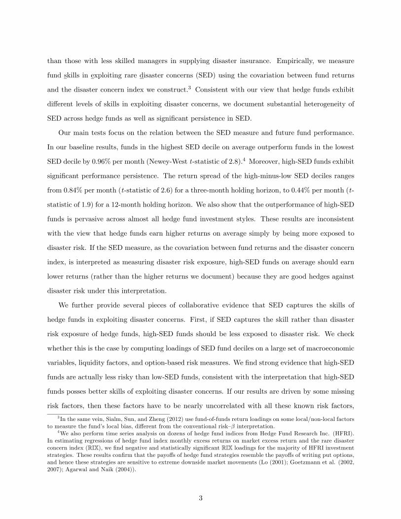
global equities, currencies, bonds, commodities, and real estates.13 Figure 2 graphs monthly high-

minus-low SED portfolio returns over the 157-month period. High-SED funds seem to outperform

low-SED funds even more during times of �nancial crisis (we present detailed subsample analysis

in Section 5.1).14

Speci�cation (2) in Table 6 reports returns for a broader sample of TASS hedge funds without

restrictions on AUM. Results are similar. High-skill funds (SED decile 10) outperform low-skill

funds (SED decile 1) by 0:89% per month (with a t-statistic of 2:7). Alphas based on the Fung-

Hsieh 8-factor model and the NPPR 10-factor models are 1:18% and 0:76% per month, respectively,

and both are signi�cant.

Bhardwaj, Gorton, and Rouwenhorst (2013) show that database back�lling introduces a sig-

ni�cant upward bias in assessing fund performance. Following their recommendation, we rely on

the date that a fund was �rst added into the TASS database to correct for the back�lling bias

in hedge fund returns (i.e., we use monthly fund returns only after this date). Speci�cation (3)

shows excess returns and alphas of SED portfolios after removing the back�lled data. Consistent

12We report estimates and Newey-West t -statistics of all factor loadings in Table IA-2 of the Internet Appendix.13The monthly alpha di¤erence (47 basis points) between the 8-factor model and the 10-factor model mainly

comes from low-SED funds: �0:63% (t -statistic = �2:8 ) under the 8-factor model vs. �0:09% (t -statistic = �0:3 ).In other words, the 10-factor model has the most signi�cant impact on adjusting the returns of low-SED funds, butnot high-SED funds.

14 In an unreported analysis, we also estimate alphas using the set of global asset pricing factors recently devel-oped in the literature, including value, momentum, betting-against-beta, and futures-based trend-following (Asness,Moskowitz, and Pedersen (2013); Frazzini and Pedersen (2014); Moskowtiz, Ooi, and Pedersen (2012); Baltas andKosowski (2012)). Our results are unchanged. The alphas of high-minus-low SED portfolios remain highly signi�cant,and they range from 0:83% to 1:20% per month depending on the model speci�cation.

16

with Bhardwaj, Gorton, and Rouwenhorst (2013), we also �nd an upward back�lling bias in fund

returns. For example, among high-skill funds (SED decile 10), such bias in�ates returns by 0:18%

(' 0:905% � 0:724%) per month, and interestingly, among low-skill funds (SED decile 1), returns

are also in�ated about 0:18% (' (�0:058%) � (�0:233%)) per month. Putting these numbers

into the perspective of average-skill funds (SED decile 5), we see the e¤ect of the back�lling bias

on fund returns is around 0:092% (= 0:264% � 0:172%). Nevertheless, removing the back�lling

hardly changes our conclusion. High-skill funds continue to outperform low-skill funds by 0:96%

per month (with a t-statistic of 2:7), and monthly alphas are 1:37% (with a t-statistic of 3:9) and

0:80% (with a t-statistic of 2:6) for the Fung-Hsieh 8-factor model and the NPPR 10-factor model,

respectively.15

The TASS database doesn�t report �delisted� hedge fund returns. We address this issue by

assuming a large negative return (such as �100%) in the month immediately after a hedge fund

exits the database for reasons such as liquidation, no longer reporting, or unable to contact fund.

The last three columns in Table 6 report portfolio results after accounting for hedge fund �delisting�

events. We �nd return patterns of SED deciles similar to those of our main result. In fact, the

return spread of the high-minus-low SED portfolio is 1:3% per month (with a t-statistic of 3:1).

Results are similar when we use di¤erent assigned values for hedge fund �delisting�returns (such as

-90%, -50%, etc.). The evidence is consistent with the earlier observation in Table 3 that high-SED

funds have lower liquidation rates.16

Overall, our results strongly suggest that hedge fund managers�skills in exploiting rare disaster

concerns play an important role in explaining their future return performance. In a nutshell, our

baseline results are inconsistent with the view that high-SED funds earn higher returns on average

simply by being more exposed to disaster risk. If the SED measure, as the covariation between fund

returns and the disaster concern index, is interpreted as measuring disaster risk exposure, high-SED

15Our results are not sensitive to how we handle back�lling bias. Following the procedure in Jagannathan,Malakhov, and Novikov (2010), we mitigate the back�lling bias by excluding the �rst 25 months from the history ofeach fund. The return spread of the high-minus-low SED portfolio is 0:89% per month (with a Newey-West t -statisticof 2:6 ), the Fung-Hsieh 8-factor alpha is 1:15% , and the NPPR 10-factor alpha is 0:81% (both are at least threestandard errors from zero).

16Relatedly, back-of-envelope calculations based on the CAPM beta of high-SED funds imply that we need apersistent market loss of 23% - 52% per year to wipe out the funds (de�ned as the fund return decreases to zero)of the three highest SED fund portfolios. The patterns are consistent with the evidence on fund liquidation ratespresented in Table 3: high-SED funds usually have lower liquidation rate (approximately 2.13% in decile 10 portfolioof funds), while low-SED funds have higher liquidation rate (about 3.56% in decile 1 portfolio of funds).

17

funds on average should earn lower returns (rather than the higher returns we document) because

they are good hedges against disaster risk under this interpretation.17 That being said, we provide

collaborative evidence that SED captures the skills of hedge funds in exploiting disaster concerns

in the following sections.

4.2 Disaster Risk Exposure

If SED captures the skill rather than disaster risk exposure of hedge funds, high-SED funds should

be less exposed to disaster risk. We check whether this is the case by computing loadings of SED

fund deciles on various measures of disaster risk. Guided by the macro-�nance literature (e.g.,

Barro (2006); Wachter (2013)), we include the following set of macroeconomic risk factors: GDP

growth, in�ation, corporate default, and term spread of bond yields. GDP growth is the real

per-capita growth rate of GDP, computed quarterly by the real GDP growth rate obtained from

the Federal Reserve Economic Data (FRED) of the Federal Reserve Bank of St. Louis and the

annual population growth obtained from the World Economic Outlook (WEO) database of the

International Monetary Fund (IMF). The in�ation rate is the monthly year-on-year percentage

change of the core consumer price index (CPI). We proxy the corporate default risk using the

di¤erence between the Moody�s Aaa and Baa corporate bond yields obtained from the FRED. We

also compute the term spread between the 10-year US Treasury yield and the 3-month T-bill rate.

We additionally consider various market and funding liquidity risk measures because liquidity

crunches often happen at the same time as macroeconomic downturns and market shocks (Brunner-

meier, Nagel, and Pedersen (2008)). The funding liquidity variables include the Treasury-Eurodollar

(TED) spread, which is equal to the 3-month LIBOR minus the 3-month T-bill rate, the LIBOR-

Repo spread, which is equal to the 3-month LIBOR minus the 3-month General Collateral Treasury

repurchase rate, and the Swap-Treasury spread, which is equal to the 10-year interest rate swap

rate minus the 10-year Treasury yield. In order to measure liquidity shocks, we take the �rst-order

17 It is also important to recognize that hedge funds are actively managed assets, and the relationship betweenrare disaster concerns and returns is di¤erent from that for passively managed assets. For example, in the context ofpassively managed assets including MSCI international equity indices, foreign currencies, global government bonds,and commodity futures, Gao and Song (2015) �nd high RIX-beta assets are favorable securities because they delivercontemporaneously higher returns when the market is fearful about rare disasters. High RIX-beta assets receivehigher demand today and their prices are being pushed up; and they subsequently earn lower returns in the future.In other words, high-RIX beta assets provide protection against market disaster concerns and the high demand frominvestors for such assets lead to lower expected returns.

18

di¤erence in each of these monthly series.18 For market liquidity, we use the on-the-run minus

the o¤-the-run 10-year Treasury yield spread obtained from the Federal Reserve Board, the level

of liquidity measure from Pastor and Stambaugh (2003), and the �noise�measure from Hu, Pan,

and Wang (2013) delineating the relative availability of arbitrage capitals. We de�ne U.S. funding

liquidity shocks, U.S. market liquidity shocks, and U.S. all liquidity shocks as the �rst principal

components based on various correlation matrices of the corresponding sets of liquidity variables.

Panel A from Table 7 reports the loadings of SED-sorted hedge fund portfolios on macroeco-

nomic and liquidity risk factors. We observe that high-SED funds are indeed less exposed to

macroeconomic and liquidity shocks than low-SED funds. The di¤erence in factor loadings is sta-

tistically signi�cant for all macro and liquidity factors, with the exception of in�ation rate. For

example, the loadings of high- and low-SED funds on default risk are �0:061 and �0:003, respec-

tively, and the di¤erence has a t-statistic of 3:4. In fact, high-SED funds are not signi�cantly

exposed to any macroeconomic and liquidity shocks.

Some readers may be concerned that general macroeconomic and liquidity risk factors are not

su¢ cient to capture disaster risk, and prefer to measure disaster risk directly using option-based

factors. In Panel B of Table 7, we consider an alternative set of risk factors based on option prices.

We regress hedge fund portfolio returns on the market excess return itself (the �rst column), and

the market excess return plus one of the following factors (the other columns): (1) volatility skew,

which is the implied volatility di¤erence between the S&P 500 index OTM put and ATM call

(Xing, Zhang, and Zhao (2010)); (2) high-order moment risk of volatility, skewness, and kurtosis

based on the S&P 500 index options (Bakshi, Kapadia, and Madan (2003)); and (3) the option

return spread between the S&P 500 index OTM and ATM puts. The patterns of loadings on these

option-based factors in Panel B are very similar to those in Panel A.19 Again, high-SED funds have

economically small and statistically insigni�cant exposure to any of these factors with the exception

of market return, and this market factor exposure is signi�cantly smaller for high-SED funds than

for low-SED funds.

Overall, factor loadings of macroeconomic and liquidity risk factors as well as option-based

18De�ning shocks as the residuals from an AR(1) or AR(2) model (e.g., Korajczyk and Sadka, 2008; Moskowitz,Ooi, and Pedersen, 2012; Asness, Moskowitz, and Pedersen, 2013) does not change our results.

19 In Table IA-3 of the Internet Appendix, we also conduct double-sorted portfolios using SED and a number offactors on market risk, downside market risk, volatility risk, macroeconomic risk, and liquidity risk. Our results showthat SED-based hedge fund performance is not driven by exposures to any of these risk factors.

19

factors show that high-SED funds are actually less risky than low-SED funds, consistent with the

interpretation of SED as capturing the skills of hedge funds in exploiting disaster concerns.

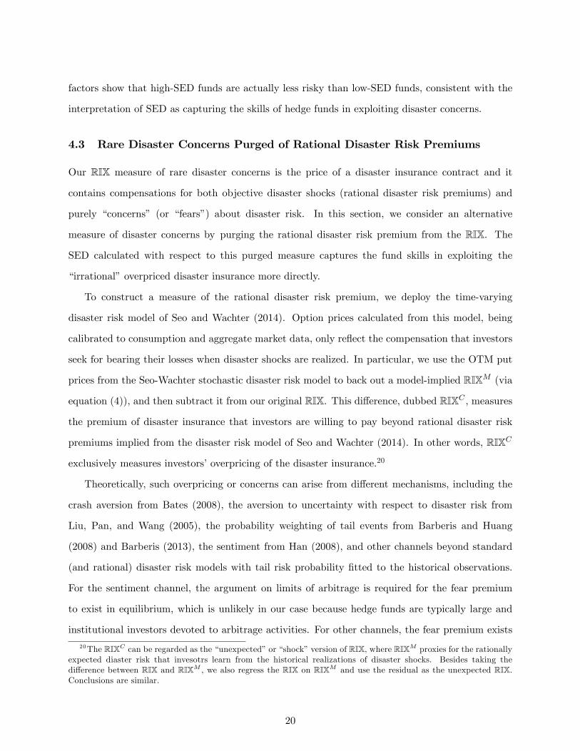
4.3 Rare Disaster Concerns Purged of Rational Disaster Risk Premiums

Our RIX measure of rare disaster concerns is the price of a disaster insurance contract and it

contains compensations for both objective disaster shocks (rational disaster risk premiums) and

purely �concerns� (or �fears�) about disaster risk. In this section, we consider an alternative

measure of disaster concerns by purging the rational disaster risk premium from the RIX. The

SED calculated with respect to this purged measure captures the fund skills in exploiting the

�irrational�overpriced disaster insurance more directly.

To construct a measure of the rational disaster risk premium, we deploy the time-varying

disaster risk model of Seo and Wachter (2014). Option prices calculated from this model, being

calibrated to consumption and aggregate market data, only re�ect the compensation that investors

seek for bearing their losses when disaster shocks are realized. In particular, we use the OTM put

prices from the Seo-Wachter stochastic disaster risk model to back out a model-implied RIXM (via

equation (4)), and then subtract it from our original RIX. This di¤erence, dubbed RIXC , measures

the premium of disaster insurance that investors are willing to pay beyond rational disaster risk

premiums implied from the disaster risk model of Seo and Wachter (2014). In other words, RIXC

exclusively measures investors�overpricing of the disaster insurance.20

Theoretically, such overpricing or concerns can arise from di¤erent mechanisms, including the

crash aversion from Bates (2008), the aversion to uncertainty with respect to disaster risk from

Liu, Pan, and Wang (2005), the probability weighting of tail events from Barberis and Huang

(2008) and Barberis (2013), the sentiment from Han (2008), and other channels beyond standard

(and rational) disaster risk models with tail risk probability �tted to the historical observations.

For the sentiment channel, the argument on limits of arbitrage is required for the fear premium

to exist in equilibrium, which is unlikely in our case because hedge funds are typically large and

institutional investors devoted to arbitrage activities. For other channels, the fear premium exists

20The RIXC can be regarded as the �unexpected�or �shock�version of RIX, where RIXM proxies for the rationallyexpected diaster risk that invesotrs learn from the historical realizations of disaster shocks. Besides taking thedi¤erence between RIX and RIXM , we also regress the RIX on RIXM and use the residual as the unexpected RIX.Conclusions are similar.

20

in equilibrium as compensation for crash aversion, uncertainty aversion, and probability weighting

of tail events. Prices of disaster insurance contracts in such models are higher than those in a

standard (and rational) disaster risk model because of the compensation for economic mechanisms

that are beyond rational disaster risk. Skilled funds are not constrained by these mechanisms in

their investment decisions, probably because they have advantage from research, information, and

experiences in understanding the economy and �nancial market better. Hence, extracting such

compensation by providing disaster insurance, funds with skills of identifying fear premium can

earn pro�ts.

We re-estimate each fund�s SED from 24-month rolling-window regressions of excess monthly

returns (with at least 18 months of fund returns available) on the market factor and the RIXC .

Then we form SED decile portfolios each month, hold them for one month, and calculate equal-

weighted returns. The �rst column of Table 8 presents the monthly returns of these decile portfolios

as well as the high-minus-low SED portfolio. Results are stronger than those of our baseline analysis

in Table 6. Under the RIXC measure, high-SED funds outperform low-SED funds by 1:21% per

month (with a Newey-West t-statistic of 3:5). Benchmarked against the NPPR 10-factor model,

respectively, alphas of the high-minus-low SED portfolio are 1:47% and 1:11% per month; both

are at least four standard errors from zero. Because the RIXC measure is free of the disaster

risk premium to the degree that the Seo-Wachter disaster risk model implies, these results provide

rea¢ rming evidence that fund managers�skills in exploiting disaster concerns drive cross-sectional

di¤erences in fund performance.21

Overall, our empirical evidence on the factor loadings of SED fund portfolios and the perfor-

mance of RIXC-based fund portfolios show that high-SED funds earn higher returns because of

their superior skills in exploiting rare disaster concerns, as opposed to simply taking greater ex-

posure to disaster risk. Finally, there is one caveat with RIXC . While we believe the theoretical

underpinning behind the construction of RIXC is valid and general, its empirical implementation

depends on the speci�cations of the disaster risk model. Thus we opt for RIX as our main measure

throughout the paper.

21We also experimented with constant disaster risk models and obtained similar results.

21

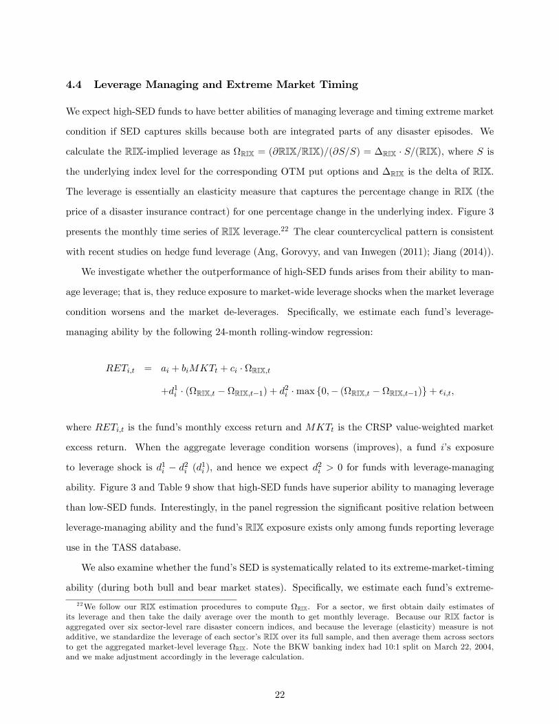
4.4 Leverage Managing and Extreme Market Timing

We expect high-SED funds to have better abilities of managing leverage and timing extreme market

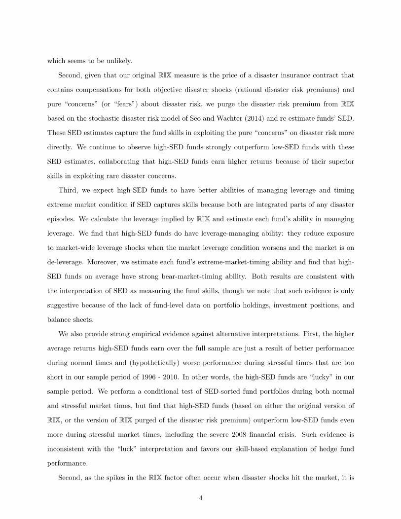
condition if SED captures skills because both are integrated parts of any disaster episodes. We

calculate the RIX-implied leverage as RIX = (@RIX=RIX)=(@S=S) = �RIX � S=(RIX), where S is

the underlying index level for the corresponding OTM put options and �RIX is the delta of RIX.

The leverage is essentially an elasticity measure that captures the percentage change in RIX (the

price of a disaster insurance contract) for one percentage change in the underlying index. Figure 3

presents the monthly time series of RIX leverage.22 The clear countercyclical pattern is consistent

with recent studies on hedge fund leverage (Ang, Gorovyy, and van Inwegen (2011); Jiang (2014)).

We investigate whether the outperformance of high-SED funds arises from their ability to man-

age leverage; that is, they reduce exposure to market-wide leverage shocks when the market leverage

condition worsens and the market de-leverages. Speci�cally, we estimate each fund�s leverage-

managing ability by the following 24-month rolling-window regression:

RETi;t = ai + biMKTt + ci � RIX;t

+d1i � (RIX;t � RIX;t�1) + d2i �max f0;� (RIX;t � RIX;t�1)g+ �i;t,

where RETi;t is the fund�s monthly excess return and MKTt is the CRSP value-weighted market

excess return. When the aggregate leverage condition worsens (improves), a fund i�s exposure

to leverage shock is d1i � d2i (d1i ), and hence we expect d2i > 0 for funds with leverage-managing

ability. Figure 3 and Table 9 show that high-SED funds have superior ability to managing leverage

than low-SED funds. Interestingly, in the panel regression the signi�cant positive relation between

leverage-managing ability and the fund�s RIX exposure exists only among funds reporting leverage

use in the TASS database.

We also examine whether the fund�s SED is systematically related to its extreme-market-timing

ability (during both bull and bear market states). Speci�cally, we estimate each fund�s extreme-

22We follow our RIX estimation procedures to compute RIX. For a sector, we �rst obtain daily estimates ofits leverage and then take the daily average over the month to get monthly leverage. Because our RIX factor isaggregated over six sector-level rare disaster concern indices, and because the leverage (elasticity) measure is notadditive, we standardize the leverage of each sector�s RIX over its full sample, and then average them across sectorsto get the aggregated market-level leverage RIX. Note the BKW banking index had 10:1 split on March 22, 2004,and we make adjustment accordingly in the leverage calculation.

22

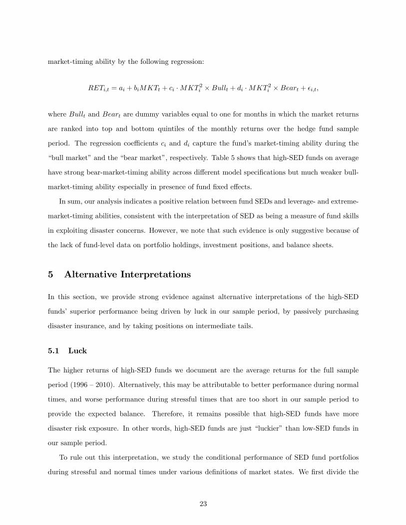
market-timing ability by the following regression:

RETi;t = ai + biMKTt + ci �MKT 2i �Bullt + di �MKT 2i �Beart + �i;t,

where Bullt and Beart are dummy variables equal to one for months in which the market returns

are ranked into top and bottom quintiles of the monthly returns over the hedge fund sample

period. The regression coe¢ cients ci and di capture the fund�s market-timing ability during the

�bull market�and the �bear market�, respectively. Table 5 shows that high-SED funds on average

have strong bear-market-timing ability across di¤erent model speci�cations but much weaker bull-

market-timing ability especially in presence of fund �xed e¤ects.

In sum, our analysis indicates a positive relation between fund SEDs and leverage- and extreme-

market-timing abilities, consistent with the interpretation of SED as being a measure of fund skills

in exploiting disaster concerns. However, we note that such evidence is only suggestive because of

the lack of fund-level data on portfolio holdings, investment positions, and balance sheets.

5 Alternative Interpretations

In this section, we provide strong evidence against alternative interpretations of the high-SED

funds� superior performance being driven by luck in our sample period, by passively purchasing

disaster insurance, and by taking positions on intermediate tails.

5.1 Luck

The higher returns of high-SED funds we document are the average returns for the full sample

period (1996 �2010). Alternatively, this may be attributable to better performance during normal

times, and worse performance during stressful times that are too short in our sample period to

provide the expected balance. Therefore, it remains possible that high-SED funds have more

disaster risk exposure. In other words, high-SED funds are just �luckier� than low-SED funds in

our sample period.

To rule out this interpretation, we study the conditional performance of SED fund portfolios

during stressful and normal times under various de�nitions of market states. We �rst divide the

23

sample period (July 1997 through July 2010) into �normal�vs. �stressful�times in four di¤erent

ways: (1) months during which the CRSP value-weighted market excess returns lose 10% or more;

(2) months in the lowest quintile when we rank all months into �ve groups based on the market

excess returns in these months; (3) normal/stressful times based on NBER recession dates (stressful

times are 28 months in total: March 2001 through November 2001, and December 2007 through

June 2009); and (4) months in the lowest/highest decile when we rank all months into ten groups

based on the market excess returns in these months. The market excess returns lose 10% or more

in six months: 10/2008, 08/1998, 11/2000, 02/2001, 09/2002, and 02/2009. The decile breakpoints

for ranking months by market excess returns are �6:5% , �3:5% , �2:0% , �0:8% , 1:1% , 1:8% ,

3:2% , 4:3% , and 6:2% .

These results are presented in speci�cations (1) - (4) of Table 10. During normal times de�ned

in speci�cations (1) - (3), high-SED funds earn higher returns than low-SED funds, ranging between

66 � 97 basis points per month, all statistically signi�cant at the 1% level. During stressful times,

all funds lose (except for certain funds in speci�cation (3)), which is consistent with the view that

hedge funds earn pro�ts overall but incur losses during market downturns as they are suppliers of

disaster insurance.23 More importantly, high-SED funds lose much less, and hence still outperform

low-SED funds. For example, in months when the market lost 10% or more, high-SED funds

outperform low-SED funds by 7:32% per month (with a t-statistic of 2:6), though they lost more

than 1:5% themselves.

Comparing SED-sorted hedge fund portfolios during �good�vs. �bad�times is also informative.

If high-SED funds outperform low-SED funds because of disaster-concern-related skills, those skills

should not be useful in explaining fund performance when the market shows fairly low disaster

concerns (e.g., bull markets) and there is simply not much space for high-SED funds to exploit.

In contrast, a risk-based story would predict otherwise. In speci�cation (4), we de�ne good times

as those months in the highest decile when we rank all months into ten groups based on market

excess returns, while bad times are those months in the lowest decile. Consistent with the skill-

23The positive returns of certain high-SED funds based on speci�cation (3) (which de�nes NBER recessions asstressful times) is due to the fact that the NBER recessions include the period of March-May 2009, when the �nancialmarket was moving up in response to the Federal Reserve�s further con�rmation of its large-scale asset purchases. Inthose three months, monthly market excess returns were 8.95%, 10.19%, and 5.21%, respectively. Removing theseperiods from the stressful times catgory leads to high-SED fund deciles earning returns insigni�cantly di¤erent fromzero. We thank Narayan Naik for suggesting alternative de�nitions of stressful periods.

24

based explanation, we observe no signi�cant return di¤erence between high- and low-SED funds

in periods of high market returns, further corroborating our SED-based explanation of hedge fund

performance.

In summary, these empirical �ndings, especially the pronounced outperformance of high-SED

funds in stressful times including the severe 2008 �nancial crisis, are inconsistent with the "luck"

interpretation and favors a skill-based explanation of hedge fund performance.24

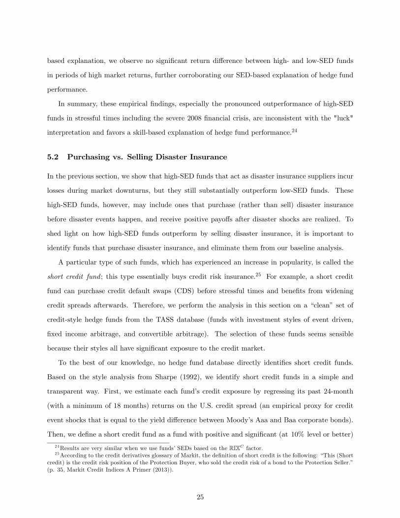
5.2 Purchasing vs. Selling Disaster Insurance

In the previous section, we show that high-SED funds that act as disaster insurance suppliers incur

losses during market downturns, but they still substantially outperform low-SED funds. These

high-SED funds, however, may include ones that purchase (rather than sell) disaster insurance

before disaster events happen, and receive positive payo¤s after disaster shocks are realized. To

shed light on how high-SED funds outperform by selling disaster insurance, it is important to

identify funds that purchase disaster insurance, and eliminate them from our baseline analysis.

A particular type of such funds, which has experienced an increase in popularity, is called the

short credit fund ; this type essentially buys credit risk insurance.25 For example, a short credit

fund can purchase credit default swaps (CDS) before stressful times and bene�ts from widening

credit spreads afterwards. Therefore, we perform the analysis in this section on a �clean� set of

credit-style hedge funds from the TASS database (funds with investment styles of event driven,

�xed income arbitrage, and convertible arbitrage). The selection of these funds seems sensible

because their styles all have signi�cant exposure to the credit market.

To the best of our knowledge, no hedge fund database directly identi�es short credit funds.

Based on the style analysis from Sharpe (1992), we identify short credit funds in a simple and

transparent way. First, we estimate each fund�s credit exposure by regressing its past 24-month

(with a minimum of 18 months) returns on the U.S. credit spread (an empirical proxy for credit

event shocks that is equal to the yield di¤erence between Moody�s Aaa and Baa corporate bonds).

Then, we de�ne a short credit fund as a fund with positive and signi�cant (at 10% level or better)

24Results are very similar when we use funds�SEDs based on the RIXC factor.25According to the credit derivatives glossary of Markit, the de�nition of short credit is the following: �This (Short

credit) is the credit risk position of the Protection Buyer, who sold the credit risk of a bond to the Protection Seller.�(p. 35, Markit Credit Indices A Primer (2013)).

25

exposure to this credit factor.

Table 11 presents the returns of SED-sorted credit-style hedge fund decile portfolios. As a

benchmark case, among credit-style hedge funds, high-SED funds outperform low-SED funds by

about 0:77% per month (with a Newey-West t-statistic of 2:6). The Fung-Hsieh and NPPR alphas

are of similar magnitudes, and both are three standard errors from zero. After excluding the short

credit funds, we �nd even stronger evidence that high-SED funds outperform low-SED funds: the

return spread of the high-minus-low SED portfolio is about 0:95% per month (with a t-statistic

of 3:0). Similarly, alphas from the Fung-Hsieh 8-factor model and the NPPR 10-factor model are

1:04% and 0:92% per month, and both are signi�cant at the 1% level. The return di¤erence

between the SED portfolios including short credit funds and those excluding short credit funds are

also signi�cant. For example, the return di¤erence between two high-minus-low SED portfolios is

about 18 basis points per month (with a t-statistic of 2:6).26

More generally, we directly test the alternative story of hedge funds�skills in purchasing disaster

insurance prior to escalated RIX: (1) (skilled) funds purchase insurance at t � 1 and outperform

from market distress at t; that is, they pay an insurance premium at t�1 to purchase the insurance

(e.g., deep-out-of-the-money put) that becomes valuable at t when the market is distressed (and

the RIX at t is high); and (2) (non-skilled) funds sell insurance at t � 1 and underperform from

market distress at t; that is, they receive an insurance premium at t� 1 to sell the insurance that

becomes toxic at t when the market is hit by a disaster shock. The returns at t� 1 of hedge funds

in the �rst (second) category should have negative (positive) loadings on RIX at t, and should earn

high (low) future returns. Empirically, we estimate each hedge fund�s exposure to rare disaster

concerns by regressing the fund�s monthly excess return at t� 1 on the next-period RIX at t, and

then examine future fund performance according to this exposure.27 We adopt the same rolling-

window speci�cation, portfolio formation, and return calculation as in our baseline analysis. The

following set of results, presented in the Internet Appendix (Tables IA-5 and IA-6), do not support

26For robustness, we also use a CDS factor in addition to the U.S. credit spread to identify short credit funds. OurCDS factor is the average of �ve CDS indices across di¤erent regions and is related to both corporate and sovereigncredit risks. The CDS indices are from Markit. Results are similar (see Table IA-4 of the Internet Appendix fordetails): the high-minus-low SED portfolio earns above 1% per month (with a t -statistic of 3:1 ) after we excludethe short credit funds from the credit-style fund sample.

27Results are similar when we use the covariance betweenregressing the fund�s monthly excess return at t� 1 onthe next-period RIX at t and the average fund return over t � 1 to t � 3, t � 1 to t � 6, t � 1 to t � 9, and t � 1 tot� 12.

26

the aforementioned alternative story: (1) low-exposure (high-exposure) funds do not earn positive

(negative) returns. They earn zero returns, both economically and statistically, during each month

over the three-month holding period after portfolio formation; (2) there is no signi�cant return

di¤erence between low- and high-exposure funds during portfolio holding periods; and (3) after we

exclude the funds that are likely to purchase disaster insurance from our sample, the SED decile

results are similar to, if not stronger than, our baseline analysis.

In summary, the analysis on disaster-insurance-purchase funds in this section corroborates our

theory that high-SED hedge funds supply disaster insurance and outperform, and these funds are

not simply repackaging portfolio insurance in one way or another.

5.3 Intermediate vs. Extreme Tails

Beside extreme tails involved in disaster concerns, hedge funds can also take positions on interme-

diate tails, which might explain the performance di¤erences of di¤erent funds. We di¤erentiate our

main result on hedge funds exploiting extreme tails from this alternative mechanism in this section.

From Section 2.1, the measure IV in (1) that underlies construction of the CBOE Volatility

Index (VIX) does not include extreme volatility shocks induced by the extreme tail events (i.e.,

those captured by RIX), as seen from (5). Therefore, we capture the intermediate tail of the market

by VIX, and use the covariation between the fund returns and VIX to capture the exploitation of

the hedge funds in intermediate tails. We then study whether SED is driven by hedge fund skills

in taking positions on intermediate tails.

The answer is unequivocally no. First, in untabulated analysis, we rank hedge funds into deciles

based on the covariation between the fund returns and VIX (analogous to SED), denoted as funds

skills in exploiting volatility concerns (SEV). We �nd no signi�cant return di¤erence between funds

with high and low SEV. The spread is 0:33% per month, with a t-statistic of 1:1. Second, in a

more direct and powerful test, we perform two sets of sequential sorts and rank hedge funds into

25 portfolios according to the SEV and SED measures. We report equal-weighted portfolio returns

in Table 12.

In Panel A, we �rst sort all funds into quintiles based on each fund�s SEV. Then we sort funds

within each SEV quintile into another �ve portfolios based on each fund�s SED. Panel A shows that

SED, even in the presence of potential fund skills in exploiting intermediate tails, well explains cross-

27

sectional hedge fund returns. On average, high-SED funds outperform low-SED funds by 0:64% per

month (t-statistic of 4:4). In fact, we observe an almost monotonically increasing relation between

SED and hedge fund returns within each quintile of SEV: The return spreads of the high-minus-low

SED portfolios range from 0:43% to 1:1% per month (all are statistically signi�cant at the 1%

level). Alphas from the 8-factor model and 10-factor model are similar in magnitude and statistical

signi�cance.

In Panel B, we �rst sort all funds into quintiles based on each fund�s SED. Then we sort funds

within each SED quintile into another �ve portfolios based on each fund�s SEV. In sharp contrast,

Panel B shows no systematic relation between SEV and hedge fund returns in the presence of SED.

On average, the return di¤erence between funds with high and low SEV is 0:11% and it is less

than one standard error from zero. Moreover, SEV has no power to explain hedge fund returns

within each SED quintile (all return spreads are economically small and statistically insigni�cant).

Alphas from the 8-factor model and 10-factor model are 0:17% and 0:11% per month, and none

of them is statistically signi�cant.28

Joenväärä and Kauppila (2015) recently propose three tail risk measures in their paper: the

total conditional tail risk (TCTR ), the systematic conditional tail risk (SCTR ), and idiosyncratic

conditional tail risk (ICTR ). At the core, all the measures are based on the simple variations of

the standard conditional expected shortfall. They further decompose TCTRi into two components

based on CAPM, and obtain SCTRi and ICTRi . In particular, SCTRi and ICTRi are calculated

as the (negated) average of systematic and idiosyncratic return, over the two months when the

market performed the worst. The idiosyncratic return is the residual of the regression, and the

systematic return is the �tted value of the regression.

These V aR -based tail risk measures are likely to capture intermediate tails for two reasons.

First, in the empirical estimation, due to short window length, the empirical measures are actual

de�ned over 8 to 9 percent V aR . Second, even if V aR is strictly de�ned over a 5% level, SCTR

and ICTR should still be interpreted as intermediate tails because a 24-month rolling window

realized returns are not designed to capture the extreme tail risk. The challenge faced by the

28 In our baseline analysis, factor loadings on Fung-Hsieh�s option-based lookback straddle factors are also revealing.First, as shown in the internet appendix (Table IA-4), high-SED funds have small and statistically insigni�cantexposure to these three option straddle factors. Second, the return di¤erence between high-SED and low-SED fundshave small and statistically insigni�cant exposure to these three option straddle factors.

28

literature on rare disaster or tail risk is that such risk can only be estimated reasonably accurate

if one extracts it from prices of tail-sensitive assets such as options, or from a long historical time

series. We will use these tail risk measures as alternatives to SEV, and carry out additional analysis.

Following Joenväärä and Kauppila (2015), we compute the SCTR and ICTR . We then con-

ducted a series of independent sorting (Table IA-2) and sequential sorting (Table IA-3) procedures

that provide direct evidence on the explanatory power of SED for fund performance in the presence

of these V aR -based tail risk measures. In summary, it is possible for high-SED funds, which mainly

exploit extreme tails, to take positions on intermediate tails. However, SED still retains its power

in explaining hedge fund returns even after controlling for SCTR and ICTR . Economically, once

we move away from the sample of funds that �mechanically�buy costly intermediate tail insurance,

which drag down the over performance, high-SED funds always outperform low-SED funds by a

large margin. Collectively, these results suggest that fund skills in exploiting concerns on extreme

rather than intermediate tails explain cross-sectional hedge fund performance.

6 Additional Analyses and Robustness Checks

In this section, we perform additional analyses and present further robustness checks on SED-sorted

hedge fund portfolios.

6.1 SED and Existing Skill Measures

We study whether our SED measure is distinct from four other fund skills recently documented in

the literature that have explanatory power for hedge fund performance. Titman and Tiu (2011)

show that skilled funds are less exposed to systematic risk, leading to a low R-squared (as the skill

measure) when one regresses fund returns on the Fung-Hsieh benchmark factors. Sun, Wang, and

Zheng (2012) argue that fund skills in pursuing unique investment strategies deliver superior per-

formance, and propose a strategy distinctiveness index (SDI) based on the correlation of individual

fund returns with the average returns of peer funds in the same style category. Cao et al. (2013)

�nd that funds that can better time the market liquidity have better performance. Finally, Sun,

Wang, and Zheng (2013) use fund returns during market downturns as a measure of fund skills in

managing downside risk, and show that such downside returns can explain cross-sectional hedge

29

fund returns.

We document the distinctiveness of the SED measure from these four documented fund skills

using the Fama-MacBeth (1973) regression. The approach allows us to control for multiple skill

measures simultaneously. Furthermore, our investigation of the characteristics of hedge funds in

forming SED deciles indicates that certain characteristics of hedge funds may be related to SED.

To account for the impact of hedge fund characteristics on future performance, we include fund

characteristics as explanatory variables in the regression. In addition, we also include di¤erent

types of betas with respect to a set of hedge fund risk factors documented in the literature.

Table 13 presents the results of regression coe¢ cients and Newey-West (1987) t-statistics when

we regress funds�monthly excess returns in month t+1 on SED and various subsets of the explana-

tory variables in month t. In all seven speci�cations, the coe¢ cients on SED decile rankings are

positive and signi�cant, showing that the explanatory power of SED on cross-sectional hedge fund

performance is not subsumed by market beta, liquidity beta, default premium beta, in�ation beta,

total variance, other fund skill variables, or other fund characteristics including assets under man-

agement (AUM), age, lagged returns, management fees, incentive fees, high water mark, personal

capital invested, leverage, lockup, and redemption notice period.

Because SED measure is empirically estimated and subject to the error-in-variable (EIV) prob-

lem, we comment on potential bias driven by EIV. First, when we regress funds�monthly excess

returns only on their SED measures, we �nd the coe¢ cient is 0:0022 (with a Newey-West t-statistic

of 2.2). It is known that the EIV problem in the context of univariate regression introduces a down-

ward bias in the estimate of coe¢ cient, and it works against us on �nding any signi�cant e¤ect

of SED. Second, to mitigate the EIV problem, we use each fund�s SED decile ranking as the re-

gressor in the Fama-MacBeth regression. Incidentally, this shrinkage-type modi�cation also makes

the coe¢ cient estimates comparable across di¤erent regression speci�cations. Third, we perform

a full set of double-sorted portfolios on SED and other variables (including other well-known skill

variables, fund characteristics, macroeconomic and liquidity risk betas). In each of the 14 cases,

we �nd both economically and statistically signi�cant SED e¤ect. We provide detailed results in

Tables IA-5 and IA-9 of the Internet Appendix. Overall, our evidence collectively suggests that the

SED e¤ect we present in the paper is unlikely to be driven by the EIV problem.

30

6.2 Performance Persistence

In Section 3.3, we �nd a strong persistence in the SED measure. A natural question is whether

funds skilled in exploiting rare disaster concerns also show persistence in their return performance.

We extend our baseline analysis of monthly SED deciles by holding them for horizons ranging

from 3 months to 18 months. To deal with returns from overlapped holding months, we follow

the independently managed portfolio approach introduced by Jegadeesh and Titman (1993) and

calculate average monthly returns. Table 14 presents the results in detail. We observe signi�cant

performance persistence up to 12 months. High-skill funds on average outperform low-skill funds

by 0:84% per month for a holding horizon of three months, 0.74% for a holding horizon of six

months, and 0:44% for a holding horizon of one year, with Newey-West t-statistics ranging from

1:9 to 2:6 . The 8-factor and 10-factor alphas of the high-minus-low SED portfolios are of similar

magnitudes and statistically signi�cance.

6.3 Pervasiveness of SED in Hedge Fund Performance

Are hedge fund skills in exploiting rare disaster concerns con�ned to particular types of hedge

funds? We examine returns from SED-sorted portfolios across di¤erent hedge fund investment

styles, and across di¤erent size groups.

Table 15 presents the results in detail. In Panel A, we sort all hedge funds into �ve SED

quintiles within each of the twelve TASS investment styles (we exclude the �other�style). For the

majority of investment styles, we observe a strong and positive relation between SED and portfolio

returns. In nine investment styles high-SED funds outperform low-SED funds; for two investment

styles (managed futures and global macro) we �nd positive but statistically insigni�cant return

di¤erences between high and low SED quintiles. The strongest outperformance by high-skill funds,

0.95% per month with a t-statistic of 2.3, is for the emerging markets investment style. The weakest

outperformance, 0.39% per month with a t-statistic of 2:9 , is for the fund-of-funds investment style.

A closer look at return patterns shows that high-SED quintiles earn signi�cantly positive returns

for all investment styles except dedicated short bias, and low-SED quintiles earn monthly excess

returns not statistically di¤erent from zero for all investment styles.

Panel B shows the strong relation between SED and fund performance across di¤erent fund size

31

groups at the time of portfolio formation (measured by net asset value, NAV). The high-minus-

low SED portfolios earn 0:96% and 0:75% per month, respectively, for funds within the lowest

and highest NAV groups, both at least three standard errors from zero.29 Finally, across all NAV

groups, all high-SED quintiles earn signi�cantly positive returns, and none of the low-SED quintiles

earns monthly excess returns di¤erent from zero. Our conclusion remains the same if we focus on

the alphas from the Fung-Hsieh 8-factor model and the NPPR 10-factor model.

In sum, the return results shown in Table 15 suggest that hedge fund skills in exploiting disaster

concerns are pervasive. For a variety of investment styles and di¤erent size groups, our evidence

suggests that high-SED funds earn high returns with their superior ability to exploit disaster

concerns and provide disaster insurance.

6.4 Value-weighted Returns, and December vs. Non-December Returns

We have focused on equal-weighted hedge fund portfolio returns throughout the paper. We ob-

tain similar results using value-weighted portfolio returns where weights are determined by funds�

monthly assets under management (AUM). Speci�cation (1) of Table 16 shows that the mean ex-

cess return and the Fung-Hsieh alpha of the high-minus-low SED portfolio are above 1% per month

with signi�cant t-statistics.30

Another issue related to hedge funds managing their reported returns is that returns during De-

cember are higher than returns during non-December months (Agarwal, Daniel, and Naik (2011)).

Speci�cation (2) of Table 16 shows that the return spreads of the high-minus-low SED portfolios

are 1:6% and 0:91% per month during December and non-December months, respectively, and

both are statistically signi�cant.

6.5 Alternative Construction of SED Measures

In our baseline analysis, we measure the fund�s SED using the RIX from 30-day options. As

an alternative, we measure rare disaster concerns using 90-day OTM puts on sector indices.31

29Our results are robust to measuring fund size by assets under management (AUM). For example, mean returnsof the high-minus-low SED portfolios within low and high AUM groups are 0.72% (with a t -statistic of 3.0) and 0.48%(with a t -statistic of 2.7), respectively.

30To preserve space, we do not tabulate results based on the 10-factor model. Our inference remains the same ifwe focus on the alphas from the 10-factor model. They are available from authors upon request.

31Throughout the paper we have constructed RIX using out-of-the-money puts on sector indices. One questionis whether a simple equal-weighted aggregated factor based on these sector-level index returns would be su¢ cient

32

Speci�cation (4) from Table 16 shows that the return spread of high-minus-low SED portfolio is

1:06% per month, which is more than three standard errors from zero. The Fung-Hsieh alpha is

larger, 1:25% per month (with a t-statistic of 4:4). We also measure rare disaster concerns using

30-day OTM puts on the S&P 500 index. Speci�cation (5) from Table 16 illustrates that the return

spread of the high-minus-low SED portfolio is 0:64% per month (with a t-statistic of 1:8) and the

Fung-Hsieh alpha is 0:96% per month (with a t-statistic of 2:6).32

6.6 Di¤erent Hedge Fund Databases

No single database completely covers the hedge fund universe. Our main results rely on hedge

funds in the Lipper TASS database, but we also examine hedge funds covered by the HFR and

CISDM databases. Our baseline results remain unchanged using these two di¤erent databases. For

example, among funds from the HFR database, high-SED funds on average outperform low-SED

funds by 0.84% per month (with a Newey-West t-statistic of 2:6). Furthermore, subsample (normal

vs. stressful times) results of fund performance of SED deciles are also similar to those we got using

the Lipper TASS database. We report details in the Internet Appendix (Tables IA-10 and IA-11).

6.7 Di¤erent Performance Metrics

Finally, in speci�cation (8) of Table 16, we examine the performance of hedge fund portfolios

sorted on SED using manipulation-proof performance measure (MPPM) developed by Goetzmann

et al. (2007), the Sharpe ratio, and the information ratio benchmarked on the Fung-Hsieh model.

A number of studies �nd that hedge funds engage in return smoothing and generate arti�cially

high Sharpe ratios and information ratios (Getmansky, Lo, and Makarov (2004); Bollen and Pool

(2008), among others). Following Getmansky, Lo, and Makarov (2004), when we estimate Sharpe

ratio and information ratio, we take into account potential hedge fund return smoothing. Similar to

the evidence based on raw and factor-model adjusted returns, these alternative performance metrics

show high-SED funds outperform low-SED funds by a signi�cant margin. For example, under the

to capture market expectations of future disaster and hence drive cross-sectional fund performance. The answer isno. Using this sector-index-return-based factor to estimate hedge funds�betas and sort funds into portfolios, we �ndthese betas have no power to explain future fund returns (full results are available upon request).

32We also construct a RIX by averaging disaster concern measures based on S&P 500 index options and sectorindex options. Results (available upon request) using this speci�cation for a rare disaster concern index are similarto those using only sector index options.

33

MPPM measure with a penalizing coe¢ cient of three, we �nd that high-SED funds have an average

MPPM of 0:065 (with a Newey-West t-statistic of 6:0), low-SED funds have an average MPPM

of �0:015 (with a t-statistic of �0:5), and the di¤erence is 0:08 (with a t-statistic of 2:5). Using

Sharpe ratios and information ratios as fund performance metrics, we �nd that high-SED funds

outperform low-SED funds by more than 40% and 35% per month, with Newey-West t-statistics

of 3:7 and 2:0 , respectively.

7 Conclusions

We provide novel evidence that hedge funds with managers who have better skills in exploiting

rare disaster concerns (SED) deliver superior future fund performance while being less exposed to

disaster risk. The key to our �nding is the di¤erentiation between ex ante market disaster concerns

and ex post disaster shocks. The former often contains a �fear premium�beyond compensations

for subsequent realized market losses. Consequently, fund managers can deliver superior future

fund performance if they are good at identifying the existence and magnitude of fear premium in

the ex ante disaster concerns, and/or identifying the investors who are willing to pay higher fear

premiums.

We develop a rare disaster concern index that equals the price of a disaster insurance contract

that re�ects the ex ante disaster concerns. We then measure fund SED based on the covariation

between fund excess returns and this index. We document substantial heterogeneity as well as

signi�cant persistence in SED. We show that funds in the highest SED decile outperform funds in

the lowest decile by 0:96% per month on average and even more during stressful market times.

High-SED funds are also shown to have less exposure to disaster risks. Overall, our results present

strong evidence that hedge fund managers with better skills in exploiting disaster concerns deliver

superior future fund performance, di¤erent from the popular view that hedge funds earn higher

average returns simply by being more exposed to disaster risk.

Who buys the insurance against rare disaster events? Are the buyers of the insurance the same

investors who also invest in the hedge funds selling such insurance? Answers to these questions may

reveal agency issues within the organization of institutional investors, and agency issues between

hedge funds and investors. We leave them for future research.

34

Appendix: Technical Details of RIX

Our rare disaster concern index quanti�es ex ante market expectations of rare disaster events

in the future. In particular, the value of RIX depends on the price di¤erence between two option-

based replication portfolios of variance swap contracts. The �rst portfolio accounts for mild market

volatility shocks, and the second for extreme volatility shocks induced by market jumps associated

with rare event risks. By construction, the RIX is essentially the price for an insurance contract

against extreme downside movements of the market in the future.

Consider an underlying asset whose time-t price is St. We assume for simplicity that the asset

does not pay dividends. An investor holding this security is concerned about its price �uctuations

over a time period [t; T ]. One way to protect herself against price changes is to buy a contract

that delivers payments equal to the extent of price variations over [t; T ], minus a prearranged price.

Such a contract is called a �variance� swap contract as the price variations are essentially about

the stochastic variance of the price process. The standard variance swap contract in practice pays

�lnSt+�St

�2+

�lnSt+2�St+�

�2+ � � �+

�ln

STST��

�2� VP (A.1)

at time T , where VP is the prearranged price of the contract. That is, the variance swap contract

uses the sum of squared log returns to measure price variations, which is a standard practice in the

�nance literature (Singleton (2006)).

For the convenience of pricing, a continuous-time setup is usually employed with �! 0 . Then

the fair price VP is

VP = EQt

(lim�!0

"�lnSt+�St

�2+

�lnSt+2�St+�

�2+ � � �+

�ln

STST��

�2#);

where Q is the risk-neutral measure. The limit inside the expectation is called quadratic variation

of the log price process, denoted as [lnS; lnS]Tt , which is the continuous-time sum of squared log

returns.

In principle, replication portfolios consisting of out-of-the-money (OTM) options written on

St can be used to replicate the time-varying payo¤ associated with the variance swap contract

and hence to determine the price VP . We now introduce two replication portfolios and their

35

implied prices for the variance swap contract. The �rst replication portfolio, which underlies the

construction of VIX by the Chicago Board Options Exchange (CBOE), focuses on the limit of the

discrete sum of squared log returns, determining VP as

IV � 2er�

�

�ZK>St

1

K2C(St;K;T )dK +

ZK<St

1

K2P (St;K;T )dK

�; (A.2)

where r is the constant risk-free rate, � � T � t is the time-to-maturity, and C(St;K;T ) and

P (St;K;T ) are prices of call and put options with strike K and maturity date T , respectively.

As seen in equation (A.2), this replication portfolio holds positions in OTM calls and puts with a

weight inversely proportional to their squared strikes. IV has been employed in the literature to

construct measures of variance risk premiums (Bollerslev, Tauchen, and Zhou (2009), Carr and Wu

(2009), and Drechsler and Yaron (2011)).

The intuition behind the construction of the second replication portfolio is that VP is equal

to the variance of the holding period log return, i.e., VP = V arQt (lnST =St) , as shown in Du and

Kapadia (2012).33 This replication portfolio relies on V arQt (lnST =St) , which avoids the discrete

sum approximation, and determines VP as

V � 2er�

�

�ZK>St

1� ln (K=St)K2

C(St;K;T )dK +

ZK<St

1� ln (K=St)K2

P (St;K;T )dK

�(A.3)

The second replication portfolio described in equation (A.3) di¤ers from the �rst replication

portfolio in equation (A.2) by assigning greater (lesser) weights to more deeply OTM put (call)

options. As the strike price K declines (increases), i.e., put (call) options become more out of the

money, 1� ln (K=St) becomes larger (smaller). As more deeply OTM options protect investors

against greater price changes, it is intuitive that the di¤erence between IV and V captures investors�

expectation about the distribution of large price variations.

To quantify the di¤erence more explicitly and obtain a measure of rare events, we assume the

33The equality VP = V arQt (lnST =St) holds exactly for processes with deterministic drift but approximately forprocesses with stochastic drift such as a stochastic volatility model. However, the approximation error is tiny for thestochastic drift case, shown by Du and Kapadia (2012) in simulations.

36

price process follows the Merton (1976) jump-di¤usion model:

dStSt

= (r � ��J) dt+ �dWt + dJt; (A.4)

where r is the constant risk-free rate, � is the volatility, Wt is a standard Brownian motion, Jt is

a compound Poisson process with jump intensity � , and the compensator for the Poisson random

measure ! [dx; dt] is equal to � 1p2��J

exp�� (x� �J)2 =2

�. The jump process Jt drives large price

variations with an average size of �J . Rare event risks, however, are not likely to be captured by

price jumps of average sizes within a range of the standard deviation �J . Instead, we focus on the

high-order moments of the Poisson random measure ! [dx; dt] , e.g., skewness and kurtosis, which

are associated with unlikely but extreme price jumps, in capturing rare event risks.

We now quantify the di¤erence between IV and V under the Merton (1976) framework. First,

as shown by Carr and Madan (1998), Demeter� et al. (1999), and Britten-Jones and Neuberger

(2000), when the price process St does not have jumps, i.e., dJt = 0 ,

IV = EQt

�Z T

t�2dt

�= VP:

That is, IV captures the price variation induced by the Brownian motion. However, for a price

process with a jump term dJt 6= 0 , it is no longer the case that IV = VP because VP now contains

price variations induced by jumps. Rather, as shown by Du and Kapadia (2012), V = VP whether

dJt is zero or not.

More important, the di¤erence between IV and V under the Merton (1976) model is (see Du

and Kapadia (2012) for a proof):

V� IV = 2EQtZ T

t

ZR0

�1 + x+ x2=2� ex

�! [dx; dt] : (A.5)

That is, V� IV captures all the high-order (� 3) moments of the Poisson random measure

! [dx; dt] associated with unlikely but extreme price jumps. In fact, equation (A.5) holds for the

entire class of Lévy processes, and approximately for stochastic volatility models with negligible

errors, as shown by Du and Kapadia (2012).

We further focus on downside rare event risks associated with unlikely but extreme negative

37

price jumps. In particular, we consider the downside versions of both IV and V:

IV� � 2er�

�

ZK<St

1

K2P (St;K;T )dK;

V� � 2er�

�

ZK<St

1� ln (K=St)K2

P (St;K;T )dK; (A.6)

where only OTM put options that protect investors against negative price jumps are used. We

then de�ne our rare disaster concern index as follows

RIX � V� � IV� = 2EQtZ T

t

ZR0

�1 + x+ x2=2� ex

�!� [dx; dt] ; (A.7)

where the second equality can be shown as similar to equation (A.5), with !� [dx; dt] the Poisson

random measure associated with negative price jumps.

38

References

Acharya, V., and L. H., Pedersen, 2005, Asset pricing with liquidity risk, Journal of Financial

Economics 77, 375-410.

Agarwal, V., G. Bakshi, and J. Huij, 2010, Do higher-moment equity risks explain hedge fund

returns?, Working paper, Georgia State University.

Agarwal, V., N. Daniel, and N. Naik, 2009, Role of Managerial Incentives and Discretion in Hedge

Fund Performance. Journal of Finance 64, 2221�56.

Agarwal, V., N. Daniel, and N. Naik, 2011, Do Hedge Funds Manage Their Reported Returns?,

Review of Financial Studies 24, 3281 - 3320.

Agarwal, V., and N. Naik, 2004, Risks and portfolio decisions involving hedge funds, Review of

Financial Studies 17, 63-98.

Aggarwal, Rajesh, and Philippe Jorion, 2010, The Performance of Emerging Hedge Funds and

Managers, Journal of Financial Economics 96, 238-256.

Ang, Andrew, Joseph Chen, and Yuhang Xing, 2006, Downside risk, Review of Financial Studies

19, 1191�1239.

Ang, Andrew, Sergiy Gorovyy, and Gregory B. van Inwegen, 2011, Hedge fund leverage, Journal

of Financial Economics 102, 102-126.

Ang, Andrew, Robert J. Hodrick, Yuhang Xing, and Xiaoyan Zhang, 2006, The cross-section of

volatility and expected returns, Journal of Finance 61, 259-299.

Aragon, George, 2007, Share Restriction and Asset Pricing: Evidence from the Hedge Fund Indus-

try, Journal of Financial Economics 83, 33�58.

Asness, Cli¤ord S., Tobias J. Moskowitz, and Lasse Heje Pedersen, 2013, Value and momentum

everywhere, Journal of Finance 68, 929-985.

Bakshi, G., N. Kapadia and D. Madan, 2003, Stock return characteristics, skew laws, and the

di¤erential pricing of individual equity options, Review of Financial Studies 16, 101-143.

Bali, Turan G., Stephen J. Brown, and Mustafa Onur Caglayan, 2011, Do hedge funds�exposures

to risk factors predict their future returns? Journal of Financial Economics 101, 36-68.

Bali, Turan G., Stephen J. Brown, and Mustafa Onur Caglayan, 2012, Systematic risk and the

cross section of hedge fund returns, Journal of Financial Economics 106, 114-131.

Baltas, A. N. and Kosowski, R.: 2012, Momentum strategies in futures markets and trend-following

funds, SSRN eLibrary.

39

Barberis, N. 2013. �The Psychology of Tail Events: Progress and Challenges�, working paper.

Barberis, N, and M. Huang. 2008. �Stocks as Lotteries: The Implications of Probability Weighting

for Security Prices.�American Economic Review 98(5): 2066-2100.

Barro, Robert J., 2006, Rare disasters and asset markets in the twentieth century, Quarterly Journal

of Economics 121, 823-866.

Bates, D., (2008). The Market for Crash Risk, Journal of Economic Dynamics and Control 32:7,

2291-2321.

Bhardwaj, Geetesh, Gary B. Gorton, and K. Geert Rouwenhorst, 2013, Fooling some of the people

all of the time: The ine¢ cient performance and persistence of commodity trading advisors, Working

Paper, Yale School of Management, Yale University.

Black, Fischer, and Myron Scholes, 1973, The pricing of options and corporate liabilities, Journal

of Political Economy 81, 637-654.

Bollen, Nicolas P. B., and Veronika K. Pool, 2008, Conditional Return Smoothing in the Hedge

Fund Industry, Journal of Financial and Quantitative Analysis 43, 267-298.

Bollerslev, Tim, George Tauchen, and Hao Zhou, 2009, Expected stock returns and variance risk

premia, Review of Financial Studies 22, 4463-4492.

Bollerslev, Tim, and Viktor Todorov, 2011, Tails, fears, and risk premia, Journal of Finance 66,

2165-2211.

Bondarenko, Oleg, 2004, Market price of variance risk and performance of hedge funds, Working

paper, University of Illinois at Chicago.

Britten-Jones, Mark, and Anthony Neuberger, 2000, Option prices, implied price processes, and

stochastic volatility, Journal of Finance 55, 839-866.

Brunnermeier, Markus K., Stefan Nagel, and Lasse Pedersen, 2008, "Carry Trades and Currency

Crashes" NBER Macroeconomics Annual, Vol. 23

Brunnermeier, Markus K., and Lasse Heje Pedersen, 2009, Market liquidity and funding liquidity,

Review of Financial Studies 22, 2201�2238.

Caballero, Ricardo J. and Arvind Krishnamurthy, 2008. �Collective Risk Management in a Flight

to Quality Episode.�Journal of Finance, Vol. 63, Issue 5, October.

Cao, Charles, Yong Chen, Bing Liang, and Andrew W. Lo, 2013, Can hedge funds time market

liquidity? Journal of Financial Economics 109(2), 493�516.

40

Carr, Peter, and Dilip Madan, 1998, Towards a theory of volatility trading, In R. Jarrow (ed.),

Volatility: New Estimation Techniques for Pricing Derivatives, chap. 29, pp. 417�27. London: Risk

Books.

Carr, Peter, and Liuren Wu, 2009, Variance risk premia, Review of Financial Studies 22, 1311-1341.

Chen, Zhuo, and Andrea Lu, 2014, A market-based funding liquidity measure, Working Paper,

Tsinghua University.

Demeter�, Kresimir, Emanuel Derman, Michael Kamal, and Joseph Zou, 1999, A guide to volatility

and variance swaps, Journal of Derivatives 6, 9-32.

Drechsler, Itamar, and Amir Yaron, 2011, What�s vol got to do with it? Review of Financial Studies

24, 1-45.

Du, Jian, and Nikunj Kapadia, 2012, Tail and volatility indices from option prices, Working paper,

University of Massachusetts.

Fama, Eugene, and James D. MacBeth, 1973, Risk, return and equilibrium: empirical tests, Journal

of Political Economy 81, 607-636.

Frazzini, A., & Pedersen, L. H. (2014). Betting against beta. Journal of Financial Economics,

111(1), 1-25.

Fung, William, and David A. Hsieh, 2001, The risk in hedge fund strategies: theory and evidence

from trend followers, Review of Financial Studies 14, 313�341.

Fung, W., D. Hsieh, N. Naik, and T. Ramadorai, 2008, Hedge Funds: Performance, Risk, and

Capital Formation, Journal of Finance 63, 1777�803.

Gabaix, Xavier, 2012, Variable rare disasters: an exactly solved framework for ten puzzles in

macro-�nance, Quarterly Journal of Economics 127, 645-700.

Gao P. G, and Z. Song, 2015, Rare Disaster Concerns Everywhere, Working Paper, Cornell Uni-

versity.

Getmansky, Mila, Andrew W. Lo, and Igor Makarov, 2004, An econometric model of serial corre-

lation and illiquidity in hedge fund returns, Journal of Financial Economics 74, 529-609.

Goetzmann, William, Jonathan Ingersoll, Matthew Spiegel, and Ivo Welch, 2002, Sharpening

Sharpe ratios, No. w9116, National Bureau of Economic Research.

Goetzmann, William, Jonathan Ingersoll, Matthew Spiegel, and Ivo Welch, 2007, Portfolio perfor-

mance manipulation and manipulation-proof performance measures, Review of Financial Studies

20, 1503-1546.

Han, B., 2008, �Investor Sentiment and Option Prices,�Review of Financial Studies, 21,387-414.

41

Hu Xing, Jun Pan, and Jiang Wang, 2013, Noise as Information for Illiquidity, Journal of Finance

68, 2223-2772.

Jagannathan, R., Malakhov, A., and Novikov,D., 2010. "Do hot hands exist among hedge fund

managers? An empirical evaluation". Journal of Finance 65, 217�255.

Jegadeesh, Narasimhan, and Sheridan Titman, 1993, Returns to buying winners and selling losers:

Implications for stock market e¢ ciency, Journal of Finance 48, 65-91.

Jiang H., and B. Kelly, 2012, Tail risk and hedge fund returns, Chicago Booth Fama�Miller Research

Paper No. 12-44.

Jiang, Wenxi, 2014, Leveraged speculators and asset prices, Working Paper, Yale University.

Joenväärä, Juha and Kauppila, Mikko, 2015, Hedge Fund Tail Risk: Performance and Hedging

Mechanisms, Working Paper, Oulu Business School.

Korajczyk, Robert A., and Ronnie Sadka, 2008, Pricing the commonality across alternative mea-

sures of liquidity, Journal of Financial Economics 87, 45-72.

Liang, B., and H. Park. 2008, Share Restriction, Liquidity Premium, and O¤shore Hedge Funds.

Working Paper, University of Massachusetts.

Li, H., X. Zhang, and R. Zhao, 2011, Investing in Talents: Manager Characteristics and Hedge

Fund Performances, Journal of Financial and Quantitative Analysis 46, 59�82.

Liu, Jun, Jun Pan, and Tan Wang, 2005, An equilibrium model of rare-event premia and its

implication for option smirks, Review of Financial Studies 18, 131-164.

Lo, Andrew W., 2001, Risk management for hedge funds: introduction and overview, Financial

Analysts Journal 57, 16�33.

Merton, Robert C., 1976, Option pricing when underlying stock returns are discontinuous, Journal

of Financial Economics 3, 125-144.

Mitchell, Mark., and Todd Pulvino, 2001, Characteristics of risk in risk arbitrage, Journal of

Finance 56, 2135�2175

Mitchell, Mark., and Todd Pulvino, 2012, Arbitrage crashes and the speed of capital, Journal of

Financial Economics 104, 469-490.

Moskowitz, T., J., Yao, H. Ooi, and L. H. Pedersen, 2012, Time series momentum, Journal of

Financial Economics 104, 228-250.

Namvar, Ethan, Phillips Blake, Pukthuanthong Kuntara, and Raghavendra P. Rau, 2014, Do Hedge

Funds Dynamically Manage Systematic Risk?, Working Paper, UC Berkley, University of Waterloo,

University of Missouri, and University of Cambridge.

42

Newey, Whitney K., and Kenneth D. West, 1987, A simple, positive semi-de�nite, heteroskedasticity

and autocorrelation consistent covariance matrix, Econometrica 55, 703-708.

Pastor, Lubos, and Robert F. Stambaugh, 2003, Liquidity risk and expected stock returns, Journal

of Political Economy 111, 642�685.

Pukthuanthong, Kuntara, and Richard Roll, 2009, Global market integration: An alternative mea-

sure and its application, Journal of Financial Economics 94(2), 214-232.

Sadka, Ronnie, 2006, Momentum and post-earnings-announcement drift anomalies: the role of

liquidity risk, Journal of Financial Economics 80, 309-349.

Sadka, Ronnie, 2010, Liquidity risk and the cross-section of hedge-fund returns, Journal of Financial

Economics 98, 54-71.

Seo, Sang Byung, and Jessica A. Wachter, 2014, Option prices in a model with stochastic disaster

risk, Working Paper, Wharton School, University of Pennsylvania.

Sharpe, William F, 1992, Asset allocation: Management style and performance measurement, The

Journal of Portfolio Management 18(2), 7-19.

Sialm, Clemens, Zheng Sun, and Lu Zheng, 2012, Home bias and local contagion: evidence from

funds of hedge funds. Working paper, University of Texas at Austin.

Singleton, Kenneth J., 2006, Empirical dynamic asset pricing, Princeton University Press.

Stulz, Rene, 2007, Hedge funds: past, present and future, Journal of Economic Perspectives 21,

175�194.

Sun, Z., Wang, A., and Zheng, L. 2012. The Road Less Traveled: Strategy Distinctiveness and

Hedge Fund Performance. Review of Financial Studies 25, 96-143.

Sun, Z., Wang, A., and Zheng, L. 2013. Only When the Tide Goes Out: Downside Returns and

Hedge Fund Performance. working paper.

Titman, S., and C. Tiu. 2011, Do the Best Hedge Funds Hedge? Review of Financial Studies 24,

123�68.

Wachter, Jessica A, 2013, Can time-varying risk of rare disasters explain aggregate stock market

volatility?, Journal of Finance 68, 987-1035.

Xing, Yuhang, Xiaoyan Zhang, and Rui Zhao, 2010, What does the individual option volatility

smirk tell us about future equity returns?, Journal of Financial and Quantitative Analysis 45(3),

641-662.

43

Table 1: Descriptive statistics of rare disaster concern indices

Panel A: Summary statistics of aggregated and sector-level rare disaster concern indicesMean Min P25 Median P75 Max Std N

KBW Banking Sector (BKX) 0.057 0.017 0.037 0.054 0.068 0.165 0.029 192PHLX Semiconductor Sector (SOX) 0.076 0.037 0.055 0.070 0.095 0.143 0.025 192PHLX Gold Silver Sector (XAU) 0.065 0.036 0.051 0.063 0.073 0.140 0.018 192PHLX Housing Sector (HGX) 0.063 0.030 0.046 0.054 0.073 0.139 0.023 114PHLX Oil Service Sector (OSX) 0.072 0.039 0.053 0.066 0.087 0.165 0.025 179PHLX Utility Sector (UTY) 0.029 0.012 0.023 0.027 0.033 0.071 0.010 165Aggregated Factor (RIX) 0.063 0.034 0.046 0.061 0.074 0.141 0.020 192

Panel B: Correlations between rare disaster concern indices and other common factorsRIX factor BKX SOX XAU HGX OSX UTY

MKTRF -0.102 -0.110 -0.013 -0.150 -0.172 -0.067 -0.177SMB 0.002 -0.019 0.087 -0.019 -0.030 -0.032 -0.051HML -0.165 -0.109 -0.112 -0.211 -0.209 -0.171 -0.032UMD -0.121 -0.202 -0.055 0.017 -0.225 -0.020 -0.080PTFSBD 0.248 0.194 0.259 0.226 0.277 0.239 0.172PTFSFX 0.051 0.073 -0.024 0.130 0.102 0.009 -0.005PTFSCOM -0.055 -0.031 -0.112 0.056 0.048 -0.083 -0.154PTFSIR 0.177 0.242 -0.029 0.163 0.348 0.091 0.069PTRSSTK -0.026 0.032 -0.114 0.017 0.139 -0.079 -0.015Liquidity risk: PS -0.193 -0.214 -0.087 -0.226 -0.325 -0.096 -0.242Liquidity risk: Sadka -0.310 -0.401 -0.130 -0.283 -0.408 -0.195 -0.220Liquidity risk: Noise -0.009 -0.046 -0.055 0.092 -0.009 0.005 0.010Change of term spread 0.222 0.251 0.169 0.167 0.280 0.141 0.259Change of default spread 0.221 0.146 0.123 0.256 0.208 0.241 0.002Change of VIX -0.094 -0.065 -0.112 -0.025 -0.048 -0.096 -0.057

Rare disaster concern indices are constructed using prices of 30-day out-of-the-money put options on different sector indices from 1996 through 2011 (see Section 2 in detail). The aggregated factor, called the rare disaster concern index (RIX), is an equal-weighted average over all sector-level rare disaster concern indices. Panel A reports summary statistics of monthly rare disaster concern indices. Panel B presents time-series correlations between one rare disaster concern index and a number of factors: Fama-French-Carhart four factors (MKTRF, SMB, HML, and UMD); Fung-Hsieh five trend-following factors (PTFSBD, PTFSFX, PTFSCOM, PTFSIR, and PTFSSTK); Pastor-Stambaugh (PS) liquidity risk factor; Sadka liquidity risk factor; Hu-Pan-Wang liquidity risk factor (noise); term risk factor (change in term spread); default risk factor (change in default spread); and volatility risk factor (change in VIX).

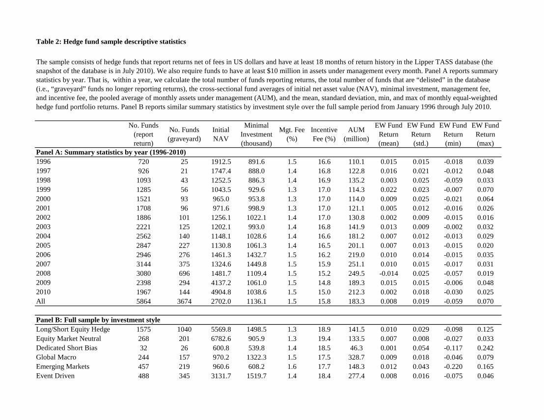
Table 2: Hedge fund sample descriptive statistics

No. Funds (report return)

No. Funds (graveyard)

Initial NAV

Minimal Investment (thousand)

Mgt. Fee (%)

Incentive Fee (%)

AUM (million)

EW Fund Return (mean)

EW Fund Return (std.)

EW Fund Return (min)

EW Fund Return (max)

Panel A: Summary statistics by year (1996-2010)1996 720 25 1912.5 891.6 1.5 16.6 110.1 0.015 0.015 -0.018 0.0391997 926 21 1747.4 888.0 1.4 16.8 122.8 0.016 0.021 -0.012 0.0481998 1093 43 1252.5 886.3 1.4 16.9 135.2 0.003 0.025 -0.059 0.0331999 1285 56 1043.5 929.6 1.3 17.0 114.3 0.022 0.023 -0.007 0.0702000 1521 93 965.0 953.8 1.3 17.0 114.0 0.009 0.025 -0.021 0.0642001 1708 96 971.6 998.9 1.3 17.0 121.1 0.005 0.012 -0.016 0.0262002 1886 101 1256.1 1022.1 1.4 17.0 130.8 0.002 0.009 -0.015 0.0162003 2221 125 1202.1 993.0 1.4 16.8 141.9 0.013 0.009 -0.002 0.0322004 2562 140 1148.1 1028.6 1.4 16.6 181.2 0.007 0.012 -0.013 0.0292005 2847 227 1130.8 1061.3 1.4 16.5 201.1 0.007 0.013 -0.015 0.0202006 2946 276 1461.3 1432.7 1.5 16.2 219.0 0.010 0.014 -0.015 0.0352007 3144 375 1324.6 1449.8 1.5 15.9 251.1 0.010 0.015 -0.017 0.0312008 3080 696 1481.7 1109.4 1.5 15.2 249.5 -0.014 0.025 -0.057 0.0192009 2398 294 4137.2 1061.0 1.5 14.8 189.3 0.015 0.015 -0.006 0.0482010 1967 144 4904.8 1038.6 1.5 15.0 212.3 0.002 0.018 -0.030 0.025All 5864 3674 2702.0 1136.1 1.5 15.8 183.3 0.008 0.019 -0.059 0.070

Panel B: Full sample by investment styleLong/Short Equity Hedge 1575 1040 5569.8 1498.5 1.3 18.9 141.5 0.010 0.029 -0.098 0.125Equity Market Neutral 268 201 6782.6 905.9 1.3 19.4 133.5 0.007 0.008 -0.027 0.033Dedicated Short Bias 32 26 600.8 539.8 1.4 18.5 46.3 0.001 0.054 -0.117 0.242Global Macro 244 157 970.2 1322.3 1.5 17.5 328.7 0.009 0.018 -0.046 0.079Emerging Markets 457 219 960.6 608.2 1.6 17.7 148.3 0.012 0.043 -0.220 0.165Event Driven 488 345 3131.7 1519.7 1.4 18.4 277.4 0.008 0.016 -0.075 0.046

The sample consists of hedge funds that report returns net of fees in US dollars and have at least 18 months of return history in the Lipper TASS database (the snapshot of the database is in July 2010). We also require funds to have at least $10 million in assets under management every month. Panel A reports summary statistics by year. That is, within a year, we calculate the total number of funds reporting returns, the total number of funds that are “delisted” in the database (i.e., “graveyard” funds no longer reporting returns), the cross-sectional fund averages of initial net asset value (NAV), minimal investment, management fee, and incentive fee, the pooled average of monthly assets under management (AUM), and the mean, standard deviation, min, and max of monthly equal-weighted hedge fund portfolio returns. Panel B reports similar summary statistics by investment style over the full sample period from January 1996 through July 2010.

Fund of Funds 1603 940 662.5 748.5 1.4 8.6 164.2 0.006 0.017 -0.062 0.063Fixed Income Arbitrage 180 151 4033.2 1106.0 1.4 19.6 255.7 0.006 0.013 -0.077 0.030Convertible Arbitrage 162 126 757.9 1120.6 1.4 18.3 183.6 0.007 0.023 -0.157 0.086Managed Futures 345 185 866.7 1092.6 2.0 19.6 201.6 0.008 0.032 -0.063 0.103Multi Strategy 324 190 1050.4 1377.0 1.6 16.3 265.4 0.008 0.015 -0.064 0.055Options Strategy 12 2 775.0 1195.8 1.5 19.6 108.6 0.006 0.011 -0.035 0.044Other 168 86 2664.2 1622.5 1.4 18.6 180.6 0.009 0.016 -0.115 0.044

Table 3: SED hedge fund portfolio characteristics

Panel A: Fund-level characteristics

Exploit Rare Disaster Concerns

AUM ($M)

AGE (Months)

Fund Flow R-squared SDI

Liquidity-Timing Ability

Market-Timing Ability

Volatility-Timing Ability

Downside Return

Upside Return

Liquidation Rate (%)

Non-Reporting Rate (%)

1 - Low Skill 172.8 68 0.010 0.533 0.305 0.059 -0.551 -0.007 -0.019 0.036 3.56 3.132 187.2 71 0.013 0.557 0.311 0.096 -0.269 -0.005 -0.011 0.024 2.77 2.543 186.7 72 0.016 0.559 0.331 0.100 -0.132 -0.008 -0.009 0.019 2.38 2.294 203.5 72 0.011 0.555 0.347 0.039 -0.126 -0.005 -0.007 0.016 2.69 1.915 193.4 71 0.015 0.546 0.362 0.014 -0.059 -0.005 -0.005 0.015 2.71 2.026 199.5 71 0.014 0.532 0.374 -0.012 -0.053 -0.004 -0.004 0.014 2.71 1.927 210.7 71 0.016 0.515 0.382 -0.018 0.059 -0.003 -0.004 0.014 2.89 2.398 192.3 70 0.044 0.505 0.382 -0.029 0.363 -0.002 -0.003 0.015 2.69 2.369 175.4 70 0.018 0.515 0.365 -0.099 0.574 -0.001 -0.004 0.019 2.46 2.33

10 - High Skill 151.2 69 0.051 0.524 0.348 -0.600 1.582 0.011 -0.005 0.028 2.13 2.25High - Low -21.6 1 0.041 -0.009 0.043 -0.659 2.133 0.018 0.014 -0.008 -1.40 -0.91

t -stat (-2.25) (0.64) (2.13) (-1.56) (6.80) (-3.43) (3.55) (3.68) (10.99) (-5.22) (-7.50) (-5.85)Sgn. Rank (p -val) (0.0068) (0.9715) (0.0000) (0.5224) (0.0000) (0.0000) (0.0028) (0.0163) (0.0000) (0.0000) (0.0000) (0.0000)

At the end of each month from June 1997 through June 2010, we rank hedge funds into ten decile portfolios according to their skills in exploiting rare disaster concerns (SED). Decile 1 (10) consists of funds with the lowest (highest) skills. In formulating portfolios, we require funds to report returns net of fees in US dollars and have at least $10 million in AUM. Funds' SEDs are estimated from 24-month rolling-window regressions of excess monthly returns on the market excess return and the level of rare disaster concerns (RIX). We also require at least 18 months of return observations in estimating regressions. Panel A reports the following hedge fund characteristics: assets under management (AUM), number of months from a fund's inception to portfolio formation date (AGE), fund flow in the recent month, R-squared based on the Fung-Hsieh factor regression in Titman and Tiu (2011), strategy distinctiveness index (SDI) in Sun, Wang, and Zheng (2012), timing ability in market liquidity, market return, and volatility in Cao et al. (2013), conditional performance measures of downside and upside returns in Sun, Wang, and Zheng (2013), and fund liquidation rate and non-reporting rate within one year of portfolio formation. Within each decile we first calculate cross-sectional average of funds' characteristics and then calculate time-series average over all portfolio formation months. We also report t -statistics and p -values of signed rank statistics for high-minus-low SED portfolios (in parentheses). Panel B reports likelihoods of 12 hedge fund investment styles that are ranked within each SED decile. Given an investment style, we estimate its odds into a SED decile as follows: We count total number of funds at portfolio formation, divide by ten to get expected number of funds (assume funds are uniformly ranked into SED deciles), estimate the ratio between realized and expected number, and calculate time-series average of the ratios over all portfolio formation months. We normalize likelihoods of all investment styles within a SED decile so that the sum of probability equals one.

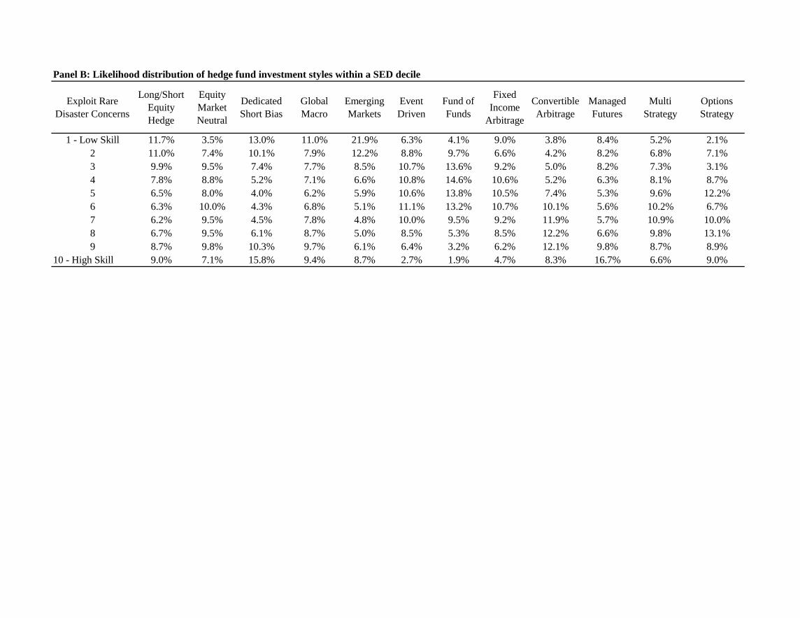
Panel B: Likelihood distribution of hedge fund investment styles within a SED decile

Exploit Rare Disaster Concerns

Long/Short Equity Hedge

Equity Market Neutral

Dedicated Short Bias

Global Macro

Emerging Markets

Event Driven

Fund of Funds

Fixed Income

Arbitrage

Convertible Arbitrage

Managed Futures

Multi Strategy

Options Strategy

1 - Low Skill 11.7% 3.5% 13.0% 11.0% 21.9% 6.3% 4.1% 9.0% 3.8% 8.4% 5.2% 2.1%2 11.0% 7.4% 10.1% 7.9% 12.2% 8.8% 9.7% 6.6% 4.2% 8.2% 6.8% 7.1%3 9.9% 9.5% 7.4% 7.7% 8.5% 10.7% 13.6% 9.2% 5.0% 8.2% 7.3% 3.1%4 7.8% 8.8% 5.2% 7.1% 6.6% 10.8% 14.6% 10.6% 5.2% 6.3% 8.1% 8.7%5 6.5% 8.0% 4.0% 6.2% 5.9% 10.6% 13.8% 10.5% 7.4% 5.3% 9.6% 12.2%6 6.3% 10.0% 4.3% 6.8% 5.1% 11.1% 13.2% 10.7% 10.1% 5.6% 10.2% 6.7%7 6.2% 9.5% 4.5% 7.8% 4.8% 10.0% 9.5% 9.2% 11.9% 5.7% 10.9% 10.0%8 6.7% 9.5% 6.1% 8.7% 5.0% 8.5% 5.3% 8.5% 12.2% 6.6% 9.8% 13.1%9 8.7% 9.8% 10.3% 9.7% 6.1% 6.4% 3.2% 6.2% 12.1% 9.8% 8.7% 8.9%

10 - High Skill 9.0% 7.1% 15.8% 9.4% 8.7% 2.7% 1.9% 4.7% 8.3% 16.7% 6.6% 9.0%

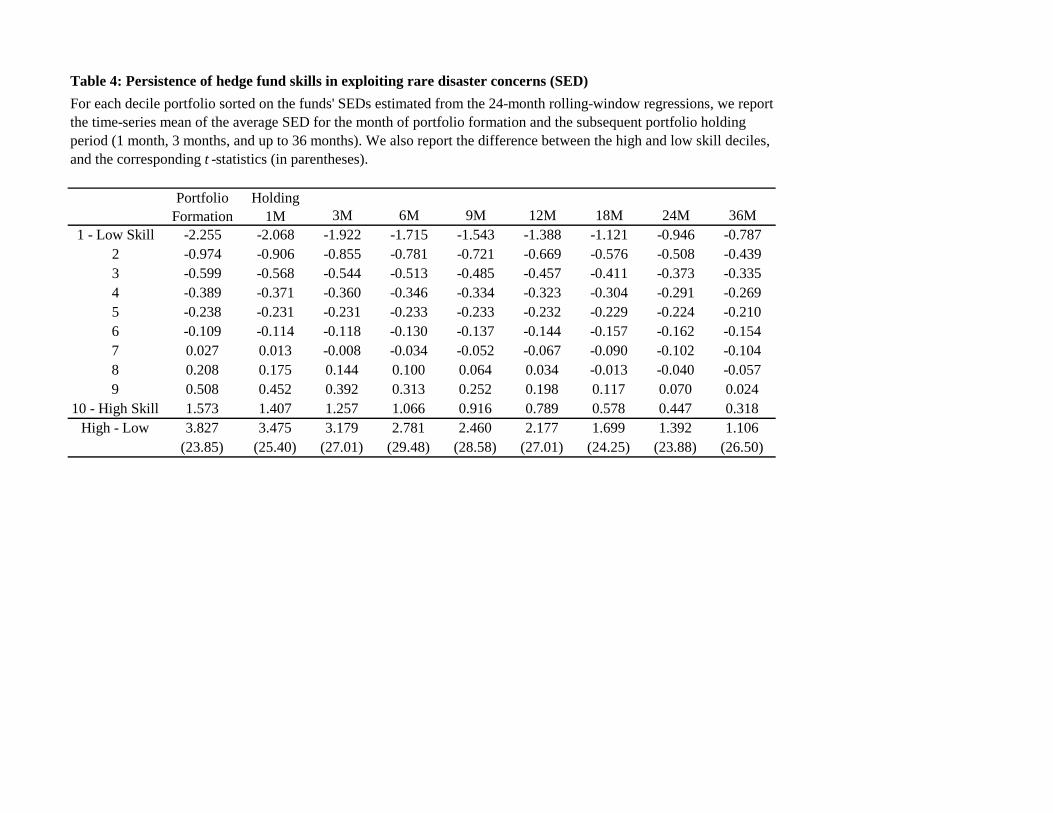
Table 4: Persistence of hedge fund skills in exploiting rare disaster concerns (SED)

Portfolio Formation

Holding 1M 3M 6M 9M 12M 18M 24M 36M

1 - Low Skill -2.255 -2.068 -1.922 -1.715 -1.543 -1.388 -1.121 -0.946 -0.7872 -0.974 -0.906 -0.855 -0.781 -0.721 -0.669 -0.576 -0.508 -0.4393 -0.599 -0.568 -0.544 -0.513 -0.485 -0.457 -0.411 -0.373 -0.3354 -0.389 -0.371 -0.360 -0.346 -0.334 -0.323 -0.304 -0.291 -0.2695 -0.238 -0.231 -0.231 -0.233 -0.233 -0.232 -0.229 -0.224 -0.2106 -0.109 -0.114 -0.118 -0.130 -0.137 -0.144 -0.157 -0.162 -0.1547 0.027 0.013 -0.008 -0.034 -0.052 -0.067 -0.090 -0.102 -0.1048 0.208 0.175 0.144 0.100 0.064 0.034 -0.013 -0.040 -0.0579 0.508 0.452 0.392 0.313 0.252 0.198 0.117 0.070 0.024

10 - High Skill 1.573 1.407 1.257 1.066 0.916 0.789 0.578 0.447 0.318High - Low 3.827 3.475 3.179 2.781 2.460 2.177 1.699 1.392 1.106

(23.85) (25.40) (27.01) (29.48) (28.58) (27.01) (24.25) (23.88) (26.50)

For each decile portfolio sorted on the funds' SEDs estimated from the 24-month rolling-window regressions, we report the time-series mean of the average SED for the month of portfolio formation and the subsequent portfolio holding period (1 month, 3 months, and up to 36 months). We also report the difference between the high and low skill deciles, and the corresponding t -statistics (in parentheses).

Table 5: Determinants of hedge fund skills in exploiting rare disaster concerns (SED)

(1) (2) (3) (4) (5) (6) (7) (8)Minimal Investment 0.029 0.020 0.0187 0.010

(2.25) (1.58) (1.49) (0.80)Management Fee (%) -5.7253 -3.604 -5.1803 -3.146

(-1.99) (-1.27) (-1.82) (-1.13)Incentive Fee (%) 0.0077 -0.067 -0.1361 -0.184

(0.03) (-0.27) (-0.56) (-0.75)Redemption Notice Period 0.0002 0.000 -0.0002 0.000

(0.40) (0.80) (-0.38) (0.01)Lockup Period -0.0022 -0.003 -0.0011 -0.002

(-1.29) (-1.67) (-0.63) (-1.02)High Water Mark 0.0541 0.052 0.0571 0.056

(1.62) (1.58) (1.72) (1.70)Personal Capital Invested -0.0157 -0.008 -0.0087 -0.002

(-0.51) (-0.25) (-0.28) (-0.05)Leverage 0.0509 0.031 0.0476 0.029

(1.85) (1.14) (1.75) (1.07)AUM -0.0291 -0.023 -0.0225 -0.017 -0.092 -0.087 -0.0514 -0.049

(-2.49) (-2.03) (-1.99) (-1.56) (-3.13) (-2.87) (-1.84) (-1.68)AGE 0.0195 0.015 0.0066 0.005 0.0044 0.007 -0.0912 -0.075

(0.64) (0.50) (0.22) (0.17) (0.07) (0.11) (-0.81) (-0.68)

We report panel regressions of SED on lagged fund characteristics using the annual data that are collected in each June from 1997 through 2010. Model specifications depend on fixed fund and year effects. We use the following explanatory variables: (1) minimal investment, AUM, and AGE are in log; (2) high water mark, personal capital invested, and leverage are dummy variables; (3) redemption notice period and lockup period are in month; (4) average monthly fund flow within the past one year; (5) monthly excess return sample moment estimates within the past two years (standard deviation, skewness, and kurtosis); and (6) a set of fund skill variables, including Fung-Hsieh alpha and R-squared, strategy distinctiveness index (SDI), downside return measure, and timing ability on market liquidity, market return, and market volatility (see Table 3 for details). The market-timing variables also contain extreme good (Bull) and extreme bad (Bear) market timing, estimated by the 18-24 month rolling-window regression for individual funds as follows: Ri,t+1 = ai + bi * MKTt+1 + ci * MKTt+1

2 * Bullt+1 + di * MKTt+12 * Beart+1 + εi,t+1, where Bull and Bear are dummy variables, equal to to one for months

in which the CRSP value-weighted market excess returns (MKT) are the top and bottom quintiles of the monthly returns over the hedge fund sample period. We report regression estimates in addition to robust t -statistics (in parenthese).

Fund Flow (past 1 year) 0.0164 0.011 0.0059 0.001 -0.0111 -0.012 -0.0368 -0.037(1.18) (0.83) (0.40) (0.07) (-0.23) (-0.27) (-0.69) (-0.73)

Return Volatility (past 2 years) 1.7971 2.737 0.6537 1.541 6.5084 8.006 2.9691 4.251(0.69) (1.04) (0.25) (0.57) (2.00) (2.58) (0.81) (1.23)

Return Skewness (past 2 years) 0.1032 0.079 0.0791 0.059 0.1703 0.140 0.1358 0.110(4.66) (3.47) (3.54) (2.57) (6.96) (5.44) (5.22) (4.03)

Return Kurtosis (past 2 years) 0.0206 0.024 0.0069 0.010 0.0043 0.008 -0.0010 0.003(2.47) (2.83) (0.81) (1.13) (0.44) (0.86) (-0.11) (0.31)

Alpha (F-H factor model) -11.1859 -10.656 -10.2262 -9.833 -14.922 -14.227 -13.8962 -13.325(-3.95) (-3.81) (-3.61) (-3.50) (-4.20) (-4.04) (-3.85) (-3.70)

R-squared (F-H factor model) 0.5228 0.409 0.4406 0.340 0.4021 0.341 0.3107 0.253(5.67) (4.56) (5.00) (3.94) (3.27) (2.86) (2.73) (2.27)

SDI 0.458 0.362 0.3408 0.251 0.3079 0.268 0.2646 0.224(4.96) (4.05) (3.70) (2.80) (2.28) (2.08) (1.99) (1.75)

Downside Return 7.2535 7.440 9.451 9.631 4.7459 5.544 6.7865 7.461(1.93) (1.98) (2.43) (2.50) (1.53) (1.85) (2.13) (2.42)

Liquidity Timing -0.0073 -0.008 -0.0178 -0.017 -0.0122 -0.013 -0.0186 -0.018(-0.62) (-0.73) (-1.44) (-1.45) (-0.76) (-0.86) (-1.15) (-1.18)

Volatility Timing -0.2435 0.500 0.0319 0.697 -0.4652 0.557 -0.3144 0.628(-0.82) (1.30) (0.10) (1.81) (-1.38) (1.37) (-0.88) (1.53)

Market Timing 0.0118 0.0104 0.0116 0.0113(2.53) (2.24) (1.75) (1.70)

Extreme Market Timing (Bullish) 0.009 0.010 0.002 0.004(2.57) (2.84) (0.52) (0.96)

Extreme Market Timing (Bearish) 0.027 0.026 0.030 0.029(7.21) (6.91) (6.99) (6.93)

Constant Included Included Included Included Included Included Included IncludedYear FEs No No Yes Yes No No Yes YesFund FEs No No No No Yes Yes Yes YesObservations 10,330 10,245 10,330 10,245 10,330 10,313 10,330 10,313Adjusted R-squared 0.0346 0.079 0.0921 0.134 0.2114 0.246 0.2550 0.286

Table 6: Return performance of SED hedge fund portfolios

Excess Ret

F-H Alpha

NPPR Alpha

Excess Ret

F-H Alpha

NPPR Alpha

Excess Ret

F-H Alpha

NPPR Alpha

Excess Ret

F-H Alpha

NPPR Alpha

1 - Low Skill -0.058 -0.628 -0.088 0.073 -0.466 0.045 -0.233 -0.900 -0.276 -0.970 -1.560 -0.912(-0.14) (-2.81) (-0.33) (0.18) (-2.40) (0.19) (-0.52) (-3.40) (-0.90) (-2.04) (-6.02) (-3.03)

2 0.195 -0.117 0.129 0.229 -0.047 0.112 0.016 -0.365 -0.007 -0.613 -0.984 -0.679(0.81) (-0.93) (0.77) (0.96) (-0.34) (0.63) (0.06) (-2.66) (-0.04) (-2.00) (-5.18) (-3.07)

3 0.294 0.008 0.241 0.292 0.024 0.204 0.229 -0.047 0.177 -0.218 -0.514 -0.219(1.45) (0.07) (1.59) (1.48) (0.22) (1.33) (1.05) (-0.36) (1.19) (-0.91) (-3.20) (-1.30)

4 0.296 0.044 0.246 0.281 0.031 0.224 0.174 -0.120 0.155 -0.279 -0.517 -0.362(1.69) (0.37) (2.06) (1.61) (0.30) (1.82) (0.88) (-0.91) (1.23) (-1.22) (-3.54) (-2.48)

5 0.264 -0.001 0.241 0.277 0.057 0.217 0.172 -0.144 0.180 -0.290 -0.567 -0.314(1.47) (-0.01) (1.98) (1.73) (0.54) (1.91) (0.87) (-0.72) (1.45) (-1.35) (-3.19) (-2.17)

6 0.280 0.090 0.228 0.272 0.073 0.227 0.206 -0.000 0.132 -0.300 -0.445 -0.328(1.87) (0.84) (2.45) (1.82) (0.70) (2.42) (1.33) (-0.00) (1.23) (-1.62) (-3.15) (-2.49)

7 0.337 0.150 0.270 0.330 0.146 0.277 0.300 0.113 0.227 -0.155 -0.355 -0.227(2.40) (1.70) (2.85) (2.40) (1.79) (3.11) (2.03) (1.19) (2.26) (-0.79) (-2.73) (-1.79)

8 0.419 0.233 0.332 0.570 0.417 0.514 0.380 0.184 0.286 -0.243 -0.454 -0.305(3.01) (2.56) (3.35) (2.89) (2.36) (2.43) (2.45) (1.72) (2.69) (-1.23) (-3.37) (-2.26)

9 0.568 0.347 0.465 0.585 0.374 0.478 0.487 0.280 0.411 -0.019 -0.255 -0.125(3.15) (2.43) (3.19) (3.47) (3.14) (3.62) (2.78) (2.03) (3.19) (-0.08) (-1.64) (-0.75)

10 - High Skill 0.905 0.668 0.735 0.967 0.752 0.825 0.724 0.498 0.547 0.334 0.098 0.160(4.17) (3.44) (3.35) (4.47) (3.97) (3.96) (3.12) (2.51) (2.40) (1.46) (0.52) (0.74)

High - Low 0.963 1.267 0.804 0.894 1.184 0.757 0.957 1.372 0.798 1.303 1.619 1.051(2.76) (3.78) (2.82) (2.70) (3.70) (2.67) (2.66) (3.86) (2.63) (3.12) (4.34) (3.17)

At the end of each month from June 1997 through June 2010, we rank hedge funds into ten decile portfolios according to their skills in exploiting rare disaster concerns (SED). Decile 1 (10) consists of funds with the lowest (highest) skills (see Table 3 for details). We hold decile portfolios for one month and calculate equally weighted returns. Monthly mean returns (in percent) and Newey-West (1987) t -statistics (in parentheses) are reported for each decile and the high-minus-low SED portfolio. We also report regression intercepts (monthly alphas) from the Fung-Hsieh 8-factor model and the Namvar-Phillips-Pukthuanthong-Rau 10-factor model, adjusted for hedge fund return smoothing as in Getmansky, Lo, and Makarov (2004). Four sets of results are presented: (1) the baseline hedge fund sample requires funds to have at least $10 million in assets under management (AUM) at the time portfolio formation (each decile on average has 147-149 funds); (2) the broader hedge fund sample has no restrictions on fund AUM (each decile on average has 264-266 funds); (3) we use the date that a fund was added into TASS database to correct for backfilling bias in hedge fund returns (each decile on average has 118-120 funds); and (4) we assume large negative returns (i.e., -100%) for all exiting funds after they are delisted in TASS database and enter into "graveyard" fund sample (each decile on average has 147-149 funds).

Exploit Rare Disaster Concerns

(1) Baseline Results (2) No AUM Restriction (3) Correct Backfilling Bias (4) Delisting Fund Return

Table 7: Risk exposure of SED hedge fund portfolios

Panel A: Macroeconomic and liquidity factor loadingsExploit Rare

Disaster Concerns

Default Risk Term Risk Real GDP

GrowthInflation

Rate

Market Liquidity

Risk

Funding Liquidity

Risk

All Liquidity

Risk1 - Low Skill -0.061 -0.008 0.008 -0.013 -0.006 -0.004 -0.005

(-3.88) (-0.95) (3.20) (-2.42) (-3.61) (-3.19) (-4.15)2 -0.044 -0.004 0.003 -0.005 -0.004 -0.003 -0.004

(-4.90) (-0.85) (2.36) (-1.40) (-4.55) (-3.65) (-4.98)3 -0.037 -0.006 0.002 -0.003 -0.003 -0.003 -0.003

(-4.84) (-1.43) (1.96) (-1.19) (-4.08) (-4.58) (-5.47)4 -0.030 -0.005 0.002 -0.002 -0.003 -0.003 -0.003

(-4.40) (-1.41) (2.25) (-0.80) (-4.13) (-4.33) (-5.32)5 -0.029 -0.003 0.002 -0.001 -0.003 -0.003 -0.003

(-3.91) (-0.74) (1.30) (-0.26) (-3.85) (-4.44) (-5.20)6 -0.025 -0.003 0.001 -0.001 -0.003 -0.002 -0.002

(-4.29) (-1.05) (1.25) (-0.36) (-4.19) (-3.81) (-4.91)7 -0.026 -0.004 0.001 -0.000 -0.003 -0.002 -0.003

(-4.55) (-1.43) (1.06) (-0.18) (-4.84) (-4.81) (-6.06)8 -0.020 0.001 0.000 -0.001 -0.002 -0.002 -0.002

(-3.46) (0.45) (0.43) (-0.60) (-3.28) (-4.22) (-4.74)9 -0.015 -0.002 -0.001 -0.001 -0.001 -0.001 -0.001

(-1.75) (-0.36) (-0.80) (-0.35) (-1.62) (-1.27) (-1.69)10 - High Skill -0.003 0.010 -0.003 -0.004 -0.000 -0.001 -0.001

(-0.23) (1.52) (-1.31) (-0.84) (-0.27) (-0.77) (-0.70)High - Low 0.058 0.018 -0.010 0.010 0.006 0.004 0.005

(3.43) (2.03) (-4.07) (1.62) (3.15) (2.37) (3.28)

We monthly form hedge fund decile portfolios based on their skills in exploiting rare disaster concerns (SED). Decile 1 (10) consists of funds with the lowest (highest) skills. We report portfolio loadings on macroeconomic and liquidity risk factors (Panel A) and disaster risk factors (Panel B). In Panel A, we regress monthly equal-weighted hedge fund portfolio returns on the market excess return and one of the following factors: (1) default risk, the change in default yield that is the difference between the Moody's Aaa and Baa corporate bond yield; (2) term risk, the change in term spread that is the difference between the 10-year T-bond yield and the 3-month T-bill rate; (3) real GDP growth that is based on the quarterly growth rate of real per-capita GDP; (4) inflation rate that is the monthly year-on-year percentage change of the consumer price index (CPI); (5) market liquidity risk that is the extracted first principal component based on the correlation matrix of the U.S. market liquidity shocks, including the on-the-run-minus-off-the-run 10-year Treasury yield spread, the Pastor and Stambaugh (2003) liquidity level, and the Hu, Pan, and Wang (2013) noise; (6) funding liquidity risk that is the extracted first principal component based on the correlation matrix of the U.S. funding liquidity shocks, including the TED spread, the LIBOR-Repo spread, and the Swap-Treasury spread; and (7) all liquidity risk that is the extracted first principal component based on the correlation matrix of all market liquidity and funding liquidity shocks in (5) and (6). We measure liquidity shocks by taking the first-order difference in each of liquidity measures above and we also define a liquidity measure such that an increased value means less liquidity. In Panel B, we regress hedge fund portfolio returns on the market excess return itself, and the market excess return and one of the following factors: (1) volatility skew that is the implied volatility difference between the S&P 500 index OTM put and ATM call as in Xing, Zhang, and Zhao (2010); (2) high-order moment risk of volatility, skewness, and kurtosis based on the S&P 500 index options as in Bakshi, Kapadia, and Madan (2003); and (3) the option return spread between the S&P 500 index OTM and ATM puts.

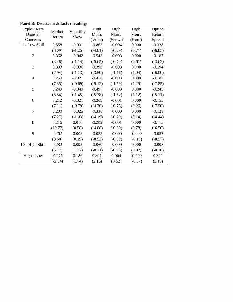
Panel B: Disaster risk factor loadingsExploit Rare

Disaster Concerns

Market Return

Volatility Skew

High Mom. (Vola.)

High Mom.

(Skew.)

High Mom. (Kurt.)

Option Return Spread

1 - Low Skill 0.558 -0.091 -0.862 -0.004 0.000 -0.328(8.09) (-1.25) (-4.01) (-0.79) (0.71) (-6.83)

2 0.362 -0.042 -0.543 -0.003 0.000 -0.187(8.48) (-1.14) (-5.65) (-0.74) (0.61) (-3.63)

3 0.303 -0.036 -0.392 -0.003 0.000 -0.194(7.94) (-1.13) (-3.50) (-1.16) (1.04) (-6.00)

4 0.250 -0.021 -0.418 -0.003 0.000 -0.181(7.35) (-0.69) (-5.12) (-1.59) (1.29) (-7.85)

5 0.249 -0.049 -0.497 -0.003 0.000 -0.245(5.54) (-1.45) (-5.38) (-1.52) (1.12) (-5.11)

6 0.212 -0.021 -0.369 -0.001 0.000 -0.155(7.11) (-0.79) (-4.30) (-0.75) (0.26) (-7.90)

7 0.200 -0.025 -0.336 -0.000 0.000 -0.128(7.27) (-1.03) (-4.19) (-0.29) (0.14) (-4.44)

8 0.216 0.016 -0.289 -0.001 0.000 -0.115(10.77) (0.58) (-4.08) (-0.80) (0.78) (-6.50)

9 0.262 0.008 -0.083 -0.000 -0.000 -0.052(8.68) (0.19) (-0.52) (-0.09) (-0.16) (-0.97)

10 - High Skill 0.282 0.095 -0.060 -0.000 0.000 -0.008(5.77) (1.37) (-0.21) (-0.08) (0.02) (-0.10)

High - Low -0.276 0.186 0.801 0.004 -0.000 0.320(-2.94) (1.74) (2.13) (0.62) (-0.57) (3.10)

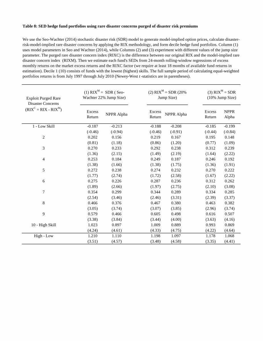
Table 8: SED hedge fund portfolios using rare disaster concerns purged of disaster risk premiums

Excess Return NPPR Alpha Excess

Return NPPR Alpha Excess Return

NPPR Alpha

1 - Low Skill -0.187 -0.213 -0.188 -0.208 -0.185 -0.199(-0.46) (-0.94) (-0.46) (-0.91) (-0.44) (-0.84)

2 0.202 0.156 0.219 0.167 0.195 0.148(0.81) (1.18) (0.86) (1.20) (0.77) (1.09)

3 0.270 0.233 0.292 0.238 0.312 0.239(1.36) (2.15) (1.49) (2.19) (1.64) (2.22)

4 0.253 0.184 0.249 0.187 0.246 0.192(1.38) (1.66) (1.38) (1.75) (1.36) (1.91)

5 0.272 0.238 0.274 0.232 0.270 0.222(1.77) (2.74) (1.72) (2.58) (1.67) (2.22)

6 0.275 0.226 0.287 0.236 0.312 0.262(1.89) (2.66) (1.97) (2.75) (2.10) (3.08)

7 0.354 0.299 0.344 0.289 0.334 0.285(2.54) (3.46) (2.46) (3.31) (2.39) (3.37)

8 0.466 0.376 0.467 0.380 0.463 0.382(3.05) (3.74) (3.07) (3.85) (2.96) (3.74)

9 0.579 0.466 0.605 0.498 0.616 0.507(3.38) (3.84) (3.44) (4.00) (3.63) (4.16)

10 - High Skill 1.023 0.897 1.009 0.889 0.993 0.869(4.24) (4.61) (4.33) (4.75) (4.22) (4.64)

High - Low 1.210 1.110 1.198 1.097 1.178 1.068(3.51) (4.57) (3.48) (4.58) (3.35) (4.41)

(1) RIXM = SDR ( Seo-Wachter 22% Jump Size)

We use the Seo-Wachter (2014) stochastic disaster risk (SDR) model to generate model-implied option prices, calculate disaster-risk-model-implied rare disaster concerns by applying the RIX methodology, and form decile hedge fund portfolios. Column (1) uses model parameters in Seo and Wachter (2014), while Columns (2) and (3) experiment with different values of the jump size parameter. The purged rare disaster concern index (RIXC) is the difference between our original RIX and the model-implied rare disaster concern index (RIXM). Then we estimate each fund's SEDs from 24-month rolling-window regressions of excess monthly returns on the market excess returns and the RIXC factor (we require at least 18 months of available fund returns in estimation). Decile 1 (10) consists of funds with the lowest (highest) skills. The full sample period of calculating equal-weighted portfolios returns is from July 1997 through July 2010 (Newey-West t -statistics are in parentheses).

Exploit Purged Rare Disaster Concerns

(RIXC = RIX - RIXM)

(2) RIXM = SDR (20% Jump Size)

(3) RIXM = SDR (10% Jump Size)

Table 9: SED relation to RIX-leverage-managing ability

RIX-Leverage Managing 0.386 0.352 1.057 0.188 0.148 0.446 0.415(2.12) (1.88) (4.44) (0.61) (0.47) (2.03) (1.84)

Minimal Investment 0.019 0.014 0.020(2.65) (2.23) (1.52)

Management Fee (%) -5.209 -9.665 -2.943(-2.17) (-3.31) (-0.95)

Incentive Fee (%) 0.583 0.769 0.505(3.31) (4.49) (1.67)

Redemption Notice Period -0.001 0.000 -0.001(-1.61) (0.53) (-2.16)

Lockup Period -0.001 -0.004 0.000(-1.12) (-2.07) (0.28)

High Water Mark 0.047 -0.060 0.119(1.67) (-1.96) (2.67)

Personal Capital Invested -0.019 -0.014 -0.021(-0.76) (-0.45) (-0.57)

Leverage 0.025(1.15)

AUM -0.047(-1.65)

AGE -0.083(-0.74)

Fund Flow (past 1 year) -0.043(-0.75)

Return Volatility (past 2 years) 3.294(0.97)

Return Skewness (past 2 years) 0.135(5.26)

Return Kurtosis (past 2 years) 0.001(0.16)

Alpha (F-H factor model) -11.669(-3.25)

R-squared (F-H factor model) 0.319(2.71)

SDI 0.249(1.86)

Downside Return 5.433(1.84)

(2) HF Reporting Leverage Use (NO)

(3) HF Reporting Leverage Use (YES)

(1) All HFs in the TASS Database (Baseline Sample)

We report panel regressions of SED on lagged fund characteristics using the annual data that are collected in each June from 1997 through 2010. Model specifications depend on fixed fund and year effects. Explanatory variables are the same as those in Table 5. Each hedge fund's RIX-leverage-managing ability is estimated by performing 24-month rolling-window regressions of fund return on the market return, the RIX leverage, the change in RIX leverage, and the maximum between zero and the negative of the change in RIX leverage (we require at least 18 months of fund returns available). The full sample consists all funds in TASS database that is used in our baseline analysis. We also choose two subsamples based on whether funds report leverage use in the TASS database. Robust t -statistics are reported in parenthese.

Liquidity Timing -0.024(-1.48)

Market Timing 0.008(1.30)

Volatility Timing -0.277(-0.80)

Year FEs No Yes Yes No Yes No YesFund FEs No No Yes No No No NoConstant Included Included Included Included Included Included IncludedObservations 20,331 20,155 10,326 8,286 8,161 12,045 11,994Adjusted R-squared 0.002 0.004 0.265 0.000 0.007 0.002 0.005

Table 10: SED-based fund performance in normal and stressful times

Full sample (07/1997 - 07/2010)

SED All 157 Months

Lost 10% or More Others Lowest

Quintile Others Stressful Times

Normal Times

Lowest Decile

Highest Decile

1 - Low Skill -0.187 -8.856 0.157 -4.310 0.868 -2.217 0.253 -6.265 2.447(-0.46) (-2.90) (0.57) (-5.27) (3.18) (-2.34) (0.79) (-4.56) (2.10)

2 0.202 -4.832 0.402 -2.596 0.918 -1.080 0.480 -3.474 1.686(0.81) (-2.95) (2.26) (-5.59) (5.53) (-1.85) (2.43) (-4.39) (1.40)

3 0.270 -3.434 0.417 -1.927 0.833 -0.978 0.541 -2.671 1.193(1.36) (-2.95) (2.90) (-5.24) (6.35) (-2.00) (3.67) (-4.36) (2.86)

4 0.253 -3.202 0.390 -1.598 0.726 -0.569 0.431 -2.268 1.304(1.38) (-2.60) (3.11) (-4.46) (6.22) (-1.33) (3.12) (-3.52) (2.58)

5 0.272 -2.673 0.389 -1.302 0.675 -0.523 0.445 -2.058 1.240(1.77) (-2.15) (3.68) (-3.82) (7.12) (-1.27) (4.00) (-3.40) (2.67)

6 0.275 -2.309 0.378 -1.261 0.668 -0.479 0.438 -1.810 1.214(1.89) (-2.08) (3.62) (-4.17) (7.04) (-1.27) (4.01) (-3.38) (2.47)

7 0.354 -1.815 0.440 -1.104 0.727 -0.264 0.488 -1.605 1.389(2.54) (-1.90) (4.19) (-3.99) (7.51) (-0.73) (4.48) (-3.30) (3.74)

8 0.466 -1.844 0.557 -1.060 0.856 -0.054 0.578 -1.423 1.749(3.05) (-2.22) (4.62) (-4.22) (7.07) (-0.16) (4.37) (-3.14) (3.49)

9 0.579 -2.032 0.683 -1.289 1.057 0.289 0.642 -1.426 2.025(3.38) (-1.97) (4.70) (-5.18) (7.03) (1.03) (3.73) (-3.13) (2.38)

10 - High Skill 1.023 -1.539 1.124 -0.952 1.528 0.815 1.068 -0.967 2.907(4.24) (-1.24) (5.05) (-2.43) (6.33) (1.66) (4.28) (-1.50) (2.95)

High - Low 1.210 7.317 0.967 3.358 0.660 3.032 0.814 5.298 0.460(3.51) (2.56) (4.23) (4.12) (2.87) (3.59) (3.29) (3.87) (0.47)

(1) Group months by market excess

returns

(2) Rank months by market excess

returns (quintiles)

(3) Group months by NBER recession

dates

(4) Rank months by market excess returns (deciles)

We classify months in four different ways and report portfolio mean excess returns (in percent) over these months (t -statistics are in parentheses): (1) months during which the CRSP value-weighted market excess returns lose 10% or more; (2) months in the lowest quintile when we rank all months into five groups based on the market excess returns in these months; (3) normal/stressful times based on NBER recession dates (stressful times are 28 months in total: March 2001 through November 2001, and December 2007 through June 2009); and (4) months in the lowest/highest decile when we rank all months into ten groups based on the market excess returns in these months. The market excess returns lose 10% or more in six months: 10/2008, 08/1998, 11/2000, 02/2001, 09/2002, and 02/2009. The decile breakpoints for ranking months by market excess returns are -6.5%, -3.5%, -2.0%, -0.8%, 1.1%, 1.8%, 3.2%, 4.3%, and 6.2%. We use the purged RIXC based on the Seo-Wachter (2014) stochastic disaster risk model and estimate each fund's SEDs from 24-month rolling-window regressions of excess monthly returns on the market excess returns and the RIXC factor (we require at least 18 months of available fund returns in estimation). Decile 1 (10) consists of funds with the lowest (highest) skills. The full sample period of calculating equal-weighted portfolios returns is from July 1997 through July 2010 (Newey-West t-statistics are in parentheses). The first column has the full-sample performance for comparison.

Table 11: SED hedge fund portfolios with versus without short credit hedge funds

Excess Ret

F-H Alpha

NPPR Alpha

Excess Ret

F-H Alpha

NPPR Alpha

Excess Ret

F-H Alpha

NPPR Alpha

1 - Low Skill 0.044 -0.215 -0.013 -0.020 -0.303 -0.069 -0.064 -0.088 -0.056(0.12) (-0.98) (-0.06) (-0.05) (-1.36) (-0.29) (-1.82) (-2.57) (-1.60)

2 0.294 0.148 0.210 0.262 0.113 0.181 -0.032 -0.035 -0.029(1.09) (0.96) (1.11) (0.97) (0.73) (0.96) (-1.84) (-1.78) (-1.76)

3 0.299 0.135 0.206 0.285 0.131 0.180 -0.014 -0.005 -0.026(1.19) (1.02) (1.25) (1.13) (1.01) (1.08) (-0.76) (-0.18) (-1.61)

4 0.321 0.200 0.217 0.301 0.177 0.199 -0.020 -0.022 -0.018(1.58) (1.93) (1.53) (1.45) (1.69) (1.37) (-1.75) (-1.93) (-1.38)

5 0.230 0.119 0.194 0.207 0.094 0.178 -0.023 -0.026 -0.017(1.38) (1.13) (1.70) (1.24) (0.86) (1.54) (-1.73) (-1.67) (-1.51)

6 0.216 0.130 0.161 0.212 0.125 0.164 -0.005 -0.005 0.003(1.35) (1.35) (1.44) (1.34) (1.29) (1.53) (-0.36) (-0.43) (0.21)

7 0.283 0.207 0.252 0.291 0.215 0.256 0.008 0.008 0.004(2.01) (2.55) (2.61) (2.03) (2.56) (2.55) (0.76) (0.84) (0.36)

8 0.472 0.360 0.383 0.466 0.345 0.368 -0.006 -0.014 -0.015(2.96) (4.04) (3.38) (2.90) (3.95) (3.25) (-0.31) (-0.64) (-0.64)

9 0.551 0.447 0.489 0.527 0.419 0.473 -0.024 -0.028 -0.017(3.96) (4.18) (4.60) (3.74) (3.73) (4.20) (-0.61) (-0.76) (-0.46)

10 - High Skill 0.813 0.633 0.731 0.926 0.737 0.855 0.113 0.105 0.124(3.76) (4.15) (4.40) (3.82) (4.14) (4.54) (1.98) (2.05) (2.20)

High - Low 0.769 0.848 0.744 0.946 1.040 0.924 0.177 0.192 0.180(2.58) (3.12) (3.02) (3.00) (3.58) (3.49) (2.59) (2.99) (2.59)

Exploit Rare Disaster Concerns

(1) Include Short Credit Funds (2) Exclude Short Credit Funds Difference (2) - (1)

Our sample of credit-style hedge funds from the TASS database consists of funds in the following investment styles: event driven, fixed income arbitrage, and convertible arbitrage. We estimate each fund's credit exposure by regressing its past 18-24 monthly returns on the U.S. credit spread (the yield difference between Moody's Aaa and Baa corporate bonds). A short credit fund is defined as the fund with positive and significant (at 10% level or better) exposure to this credit factors. Such a fund has positive payoffs when disaster shocks are realized in the credit market and essentially purchases credit protections before stressful market times. At the end of each month from June 1997 through June 2010, we rank our sample of credit-style hedge funds into decile portfolios according to their skills in exploiting rare disaster concerns (SED). We hold portfolios for one month and calculate equally weighted returns. Monthly mean returns (in percent) and Newey-West (1987) t -statistics (in parentheses) are reported, in addition to alphas from the Fung-Hsieh 8-factor model and the Namvar-Phillips-Pukthuanthong-Rau 10-factor model. The first (second) section presents results of portfolios including (excluding) short credit funds, and the last section tests the return difference. On average, each SED decile has 35-36 funds when short credit funds are included, and 26-32 funds when short credit funds are excluded.

Table 12: Return performance of SEV and SED 25 portfolios

Panel A: 5×5 portfolios based on sequential sorts first on SEV and then on SEDExploiting Volatility Concerns

1 - Low Skill 2 3 4 5 - High

Skill 5-1 F-H Alpha NPPR Alpha

1 - low 0.111 0.330 0.505 0.941 1.183 1.073 1.158 0.892(0.36) (1.47) (2.32) (3.58) (3.36) (4.30) (4.41) (3.52)

2 0.067 0.277 0.259 0.479 0.639 0.572 0.729 0.528(0.29) (2.06) (1.77) (3.59) (3.19) (3.40) (4.56) (3.17)

3 0.103 0.194 0.297 0.359 0.629 0.526 0.586 0.509(0.58) (1.54) (2.79) (3.69) (4.35) (3.71) (4.21) (3.67)

4 0.137 0.279 0.242 0.260 0.566 0.429 0.556 0.364(0.72) (2.23) (2.19) (2.45) (4.82) (3.19) (4.67) (3.10)

5 - High -0.092 0.032 0.107 0.286 0.524 0.616 0.818 0.648(-0.30) (0.17) (0.61) (2.02) (3.29) (2.47) (3.65) (2.73)

Average 0.065 0.223 0.282 0.465 0.708 0.643 0.770 0.588(0.30) (1.56) (2.06) (3.50) (4.14) (4.44) (5.65) (4.29)

Panel B: 5×5 portfolios based on sequential sorts first on SED and then on SEVExploiting Disaster Concerns

1 - Low Skill 2 3 4 5 - High

Skill 5-1 F-H Alpha NPPR Alpha

1 - Low Skill -0.260 0.137 0.125 0.003 0.017 0.277 0.312 0.208(-0.83) (0.65) (0.69) (0.01) (0.06) (0.97) (1.13) (0.73)

2 0.116 0.287 0.213 0.308 0.334 0.218 0.262 0.232(0.57) (2.09) (1.74) (2.65) (2.65) (1.36) (1.70) (1.55)

3 0.201 0.245 0.264 0.320 0.419 0.218 0.276 0.240(1.04) (1.94) (2.45) (3.34) (3.92) (1.65) (2.48) (2.34)

4 0.389 0.371 0.388 0.429 0.513 0.124 0.220 0.117(1.92) (2.56) (3.09) (3.72) (4.22) (0.85) (1.80) (0.93)

5 - High Skill 1.035 0.799 0.660 0.680 0.752 -0.283 -0.242 -0.226(2.90) (3.08) (3.09) (3.68) (3.61) (-1.10) (-0.96) (-0.95)

Average 0.296 0.368 0.330 0.348 0.407 0.111 0.166 0.114(1.27) (2.29) (2.43) (2.78) (2.91) (0.73) (1.26) (0.89)

At the end of each month from June 1997 through June 2010, we employ sequential sorts and rank hedge funds into 25 portfolios according to their skills on exploiting volatility concerns (SEV) and skills on exploiting disaster concerns (SED). We hold portfolios for one month and calculate equal-weighted portfolio returns. Hedge fund skills are estimated on 24-month rolling-window regression of funds’ excess monthly returns on the market factor, the CBOE Volatility Index (VIX) factor, and the RIX factor (with at least 18-month return observations available). This table presents portfolios’ monthly mean excess returns (in percent) and Newey-West (1987) t -statistics (in parentheses). In Panel A, we report average returns of SED quintiles after controlling for SEV effect; in Panel B, we report average returns of SEV quintiles after controlling for SED effect. The last two columns of each panel report high-minus-low SED portfolios' alphas based on the Fung-Hsieh 8-factor model and the Namvar-Phillips-Pukthuanthong-Rau 10-factor model.

Table 13: Fama-MacBeth regressions of hedge fund returns

(1) (2) (3) (4) (5) (6) (7)SED 0.0005 0.0004 0.0004 0.0004 0.0003 0.0004 0.0005

(2.41) (2.47) (2.48) (2.65) (2.11) (2.50) (3.03)Market Beta 0.0024 0.0036 0.0030 0.0033 0.0061 0.0056 0.0021

(0.63) (1.14) (0.94) (1.07) (1.87) (1.77) (0.49)Liquidity Beta -0.1498

(-2.04)Default Premium Beta 0.0058

(0.72)Inflation Beta -0.1052

(-2.12)Total Variance 0.0480

(0.37)Skewness 0.0005

(1.83)Kurtosis -0.0001

(-1.51)Downside Return 0.0934 0.0958

(2.62) (2.63)R-Squared -0.0022

(-0.80)SDI -0.0023

(-0.97)Liquidity Timing 0.0000

(-0.16)Market Timing 0.0002

This table reports results from Fama-MacBeth (1973) cross-sectional regressions of hedge funds’ excess returns in month t +1 on their SED decile rankings and other explanatory variables as of month t . The sample consists of funds that report returns net of fees in US dollars and have at least $10 million AUM. Funds’ market beta and SED are estimated from 24-month rolling-window regressions of funds’ excess monthly returns on market excess return and the measure of rare disaster concerns (RIX). Other betas are estimated in a similar way. That is, to estimate liquidity beta, default premium beta, and inflation beta, we regress fund’s excess returns on the Hu-Pan-Wang noise factor, default spreads, and inflation, respectively, in presence of the controls of market excess return and the RIX. We also require at least 18 months of return observations in estimating regressions. Funds’ characteristic variables include total variance, skewness, and kurtosis (the sample variance, skewness, and kurtosis estimates of fund’s excess returns within the past 24 months, respectively), AUM (the log of assets under management), AGE (the log of fund’s age that equals number of months from inception to month t ), lagged return (the fund’s excess return in month t ), management fee, incentive fee, four dummy variables (high water mark requirement, personal capital invested, leverage used, and lockup requirement), and redemption notice period. Funds’ skill variables include R-squared based on the Fung-Hsieh factor regression in Titman and Tiu (2011), strategy distinctiveness index (SDI) in Sun, Wang, Zheng (2012), timing ability in market liquidity, market return, and market volatility in Cao et al. (2013), and downside return measure in Sun, Wang, Zheng (2013). We report the time-series average of Fama-MacBeth regression coefficients and Newey-West (1987) t -statistics (in parentheses).

(1.25)Volatility Timing -0.0384

(-1.94)AUM -0.0003 -0.0003 -0.0003 -0.0003 -0.0005 -0.0002

(-1.75) (-1.77) (-1.70) (-1.59) (-2.05) (-0.97)AGE -0.0002 -0.0002 -0.0003 -0.0001 -0.0002 -0.0004

(-0.82) (-0.79) (-1.01) (-0.29) (-0.74) (-1.34)Lagged Return 0.1144 0.1022 0.1101 0.1076 0.1064 0.1116

(7.36) (6.25) (7.12) (7.01) (7.08) (5.14)Management Fee 0.0849 0.0793 0.0847 0.0772 0.1241 0.0890

(1.97) (1.88) (2.05) (1.88) (2.70) (2.35)Incentive Fee 0.0057 0.0059 0.0063 0.0051 0.0087 0.0031

(2.72) (2.90) (2.80) (2.41) (2.31) (1.34)High Water Mark 0.0012 0.0011 0.0012 0.0010 0.0009 0.0013

(3.50) (3.25) (3.49) (2.98) (2.32) (3.27)Personal Capital Invested 0.0003 0.0003 0.0003 0.0003 0.0002 0.0003

(1.17) (1.20) (1.19) (1.15) (0.56) (1.09)Leverage Used 0.0006 0.0006 0.0005 0.0006 0.0006 0.0004

(2.03) (1.92) (1.69) (1.81) (1.30) (1.34)Lockup Required 0.0012 0.0012 0.0012 0.0006 0.0007 0.0003

(3.59) (3.52) (3.49) (1.72) (1.68) (1.19)Redemption Notice Period 0.0000 0.0000 0.0000 0.0000 0.0000 0.0000

(1.51) (1.55) (1.49) (1.24) (1.04) (2.03)Intercept 0.0001 -0.0015 -0.0016 -0.0017 -0.0013 -0.0001 -0.0021

(0.06) (-0.84) (-0.86) (-1.01) (-0.81) (-0.02) (-1.21)Avg # of funds per month 1485 1480 1480 1480 1335 995 1212Avg adjusted R-sqr 0.157 0.210 0.228 0.235 0.249 0.233 0.240Number of months 157 157 157 157 157 157 151

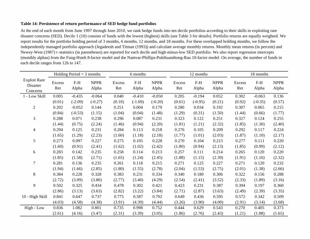
Table 14: Persistence of return performance of SED hedge fund portfolios

Exploit Rare Disaster

Concerns

Excess Ret

F-H Alpha

NPPR Alpha

Excess Ret

F-H Alpha

NPPR Alpha

Excess Ret

F-H Alpha

NPPR Alpha

Excess Ret

F-H Alpha

NPPR Alpha

1 - Low Skill 0.005 -0.435 -0.064 0.040 -0.410 -0.050 0.205 -0.194 0.052 0.302 -0.063 0.136(0.01) (-2.09) (-0.27) (0.10) (-1.69) (-0.20) (0.61) (-0.95) (0.21) (0.92) (-0.35) (0.57)

2 0.202 -0.052 0.144 0.251 0.004 0.179 0.280 0.034 0.192 0.307 0.065 0.215(0.84) (-0.53) (1.15) (1.04) (0.04) (1.48) (1.29) (0.31) (1.50) (1.44) (0.66) (1.77)

3 0.288 0.071 0.238 0.296 0.087 0.231 0.323 0.122 0.251 0.327 0.124 0.255(1.44) (0.75) (2.24) (1.46) (0.94) (2.20) (1.81) (1.21) (2.32) (1.85) (1.30) (2.40)

4 0.294 0.125 0.231 0.284 0.113 0.218 0.276 0.105 0.209 0.292 0.117 0.224(1.65) (1.29) (2.23) (1.60) (1.18) (2.18) (1.77) (1.01) (2.03) (1.87) (1.10) (2.17)

5 0.273 0.097 0.227 0.275 0.105 0.228 0.270 0.104 0.215 0.277 0.111 0.220(1.60) (0.91) (2.41) (1.62) (1.02) (2.42) (1.80) (0.94) (2.13) (1.85) (0.99) (2.12)

6 0.283 0.142 0.235 0.258 0.114 0.213 0.257 0.111 0.214 0.265 0.120 0.220(1.85) (1.58) (2.71) (1.65) (1.24) (2.45) (1.88) (1.15) (2.39) (1.91) (1.16) (2.32)

7 0.281 0.136 0.235 0.261 0.118 0.215 0.271 0.125 0.227 0.271 0.120 0.232(1.94) (1.66) (2.85) (1.80) (1.55) (2.78) (2.04) (1.53) (2.75) (2.01) (1.38) (2.66)

8 0.384 0.228 0.328 0.383 0.231 0.334 0.340 0.180 0.306 0.322 0.156 0.288(2.72) (3.09) (3.80) (2.77) (3.40) (4.29) (2.54) (2.41) (3.52) (2.33) (1.89) (3.16)

9 0.502 0.325 0.434 0.478 0.302 0.421 0.423 0.231 0.387 0.394 0.197 0.360(2.86) (3.13) (3.63) (2.82) (3.22) (3.84) (2.71) (2.87) (3.63) (2.49) (2.39) (3.35)

10 - High Skill 0.841 0.647 0.737 0.775 0.587 0.702 0.649 0.436 0.595 0.572 0.342 0.509(4.03) (4.58) (4.38) (3.91) (4.39) (4.44) (3.26) (3.90) (4.00) (2.91) (3.14) (3.68)

High - Low 0.836 1.082 0.801 0.735 0.998 0.752 0.444 0.629 0.543 0.270 0.405 0.373(2.61) (4.16) (3.47) (2.31) (3.39) (3.05) (1.86) (2.76) (2.43) (1.21) (1.88) (1.65)

18 monthsHolding Period = 3 months 6 months 12 months

At the end of each month from June 1997 through June 2010, we rank hedge funds into ten decile portfolios according to their skills in exploiting rare disaster concerns (SED). Decile 1 (10) consists of funds with the lowest (highest) skills (see Table 3 for details). Portfolio returns are equally weighted. We report results for the portfolio holding period of 3 months, 6 months, 12 months, and 18 months. For these overlapped holding months, we follow the independently managed portfolio approach (Jegadeesh and Titman (1993)) and calculate average monthly returns. Monthly mean returns (in percent) and Newey-West (1987) t -statistics (in parentheses) are reported for each decile and high-minus-low SED portfolio. We also report regression intercepts (monthly alphas) from the Fung-Hsieh 8-factor model and the Namvar-Phillips-Pukthuanthong-Rau 10-factor model. On average, the number of funds in each decile ranges from 126 to 147.

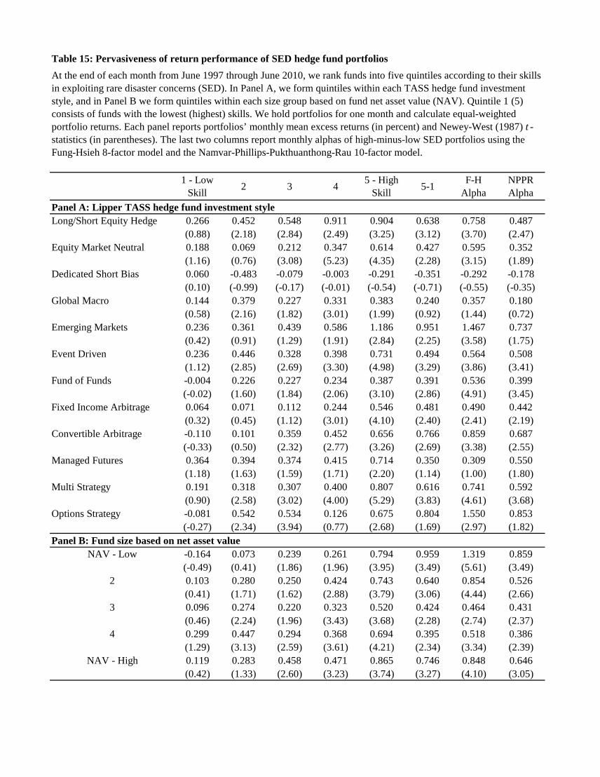
Table 15: Pervasiveness of return performance of SED hedge fund portfolios

1 - Low Skill 2 3 4 5 - High

Skill 5-1 F-H Alpha

NPPR Alpha

Panel A: Lipper TASS hedge fund investment styleLong/Short Equity Hedge 0.266 0.452 0.548 0.911 0.904 0.638 0.758 0.487

(0.88) (2.18) (2.84) (2.49) (3.25) (3.12) (3.70) (2.47)Equity Market Neutral 0.188 0.069 0.212 0.347 0.614 0.427 0.595 0.352

(1.16) (0.76) (3.08) (5.23) (4.35) (2.28) (3.15) (1.89)Dedicated Short Bias 0.060 -0.483 -0.079 -0.003 -0.291 -0.351 -0.292 -0.178

(0.10) (-0.99) (-0.17) (-0.01) (-0.54) (-0.71) (-0.55) (-0.35)Global Macro 0.144 0.379 0.227 0.331 0.383 0.240 0.357 0.180

(0.58) (2.16) (1.82) (3.01) (1.99) (0.92) (1.44) (0.72)Emerging Markets 0.236 0.361 0.439 0.586 1.186 0.951 1.467 0.737

(0.42) (0.91) (1.29) (1.91) (2.84) (2.25) (3.58) (1.75)Event Driven 0.236 0.446 0.328 0.398 0.731 0.494 0.564 0.508

(1.12) (2.85) (2.69) (3.30) (4.98) (3.29) (3.86) (3.41)Fund of Funds -0.004 0.226 0.227 0.234 0.387 0.391 0.536 0.399

(-0.02) (1.60) (1.84) (2.06) (3.10) (2.86) (4.91) (3.45)Fixed Income Arbitrage 0.064 0.071 0.112 0.244 0.546 0.481 0.490 0.442

(0.32) (0.45) (1.12) (3.01) (4.10) (2.40) (2.41) (2.19)Convertible Arbitrage -0.110 0.101 0.359 0.452 0.656 0.766 0.859 0.687

(-0.33) (0.50) (2.32) (2.77) (3.26) (2.69) (3.38) (2.55)Managed Futures 0.364 0.394 0.374 0.415 0.714 0.350 0.309 0.550

(1.18) (1.63) (1.59) (1.71) (2.20) (1.14) (1.00) (1.80)Multi Strategy 0.191 0.318 0.307 0.400 0.807 0.616 0.741 0.592

(0.90) (2.58) (3.02) (4.00) (5.29) (3.83) (4.61) (3.68)Options Strategy -0.081 0.542 0.534 0.126 0.675 0.804 1.550 0.853

(-0.27) (2.34) (3.94) (0.77) (2.68) (1.69) (2.97) (1.82)Panel B: Fund size based on net asset value

NAV - Low -0.164 0.073 0.239 0.261 0.794 0.959 1.319 0.859(-0.49) (0.41) (1.86) (1.96) (3.95) (3.49) (5.61) (3.49)

2 0.103 0.280 0.250 0.424 0.743 0.640 0.854 0.526(0.41) (1.71) (1.62) (2.88) (3.79) (3.06) (4.44) (2.66)

3 0.096 0.274 0.220 0.323 0.520 0.424 0.464 0.431(0.46) (2.24) (1.96) (3.43) (3.68) (2.28) (2.74) (2.37)

4 0.299 0.447 0.294 0.368 0.694 0.395 0.518 0.386(1.29) (3.13) (2.59) (3.61) (4.21) (2.34) (3.34) (2.39)

NAV - High 0.119 0.283 0.458 0.471 0.865 0.746 0.848 0.646(0.42) (1.33) (2.60) (3.23) (3.74) (3.27) (4.10) (3.05)

At the end of each month from June 1997 through June 2010, we rank funds into five quintiles according to their skills in exploiting rare disaster concerns (SED). In Panel A, we form quintiles within each TASS hedge fund investment style, and in Panel B we form quintiles within each size group based on fund net asset value (NAV). Quintile 1 (5) consists of funds with the lowest (highest) skills. We hold portfolios for one month and calculate equal-weighted portfolio returns. Each panel reports portfolios’ monthly mean excess returns (in percent) and Newey-West (1987) t -statistics (in parentheses). The last two columns report monthly alphas of high-minus-low SED portfolios using the Fung-Hsieh 8-factor model and the Namvar-Phillips-Pukthuanthong-Rau 10-factor model.

Table 16: Robustness checks on SED hedge fund portfolios

Exploit Rare Disaster

Concerns

Excess Ret

F-H Alpha

Excess Ret

F-H Alpha

Excess Ret

F-H Alpha

Excess Ret

F-H Alpha

Excess Ret

F-H Alpha

Excess Ret F-H Alpha Excess

Ret F-H Alpha MPPM Sharpe Ratio

Inform. Ratio

1 - Low Skill -0.165 -0.606 -0.181 -0.530 1.297 -0.230 -0.128 -0.562 -0.093 -0.576 0.080 -0.335 -0.005 -0.236 -0.015 0.148 0.173(-0.43) (-2.49) (-0.42) (-2.35) (2.54) (-0.47) (-0.33) (-2.78) (-0.26) (-2.19) (0.20) (-1.78) (-0.01) (-1.24) (-0.46) (1.04) (1.00)

2 0.127 -0.179 0.096 -0.077 1.290 0.899 0.186 -0.055 0.353 0.050 0.263 0.024 0.284 0.185 0.026 0.221 0.189(0.44) (-1.05) (0.38) (-0.75) (3.28) (1.31) (0.80) (-0.48) (1.54) (0.34) (1.06) (0.25) (1.09) (1.34) (1.55) (1.56) (1.41)

3 0.276 0.054 0.191 0.039 1.439 0.439 0.287 0.078 0.087 -0.184 0.325 0.118 0.388 0.289 0.033 0.320 0.248(1.28) (0.42) (0.91) (0.40) (4.11) (1.40) (1.44) (0.76) (0.36) (-1.01) (1.56) (1.19) (1.79) (2.42) (2.65) (2.28) (1.69)

4 0.382 0.231 0.226 0.100 1.064 0.526 0.225 0.033 0.359 0.143 0.295 0.114 0.272 0.185 0.036 0.320 0.355(2.25) (2.10) (1.25) (0.94) (3.90) (1.46) (1.28) (0.31) (2.10) (1.36) (1.65) (1.31) (1.54) (2.02) (3.28) (2.24) (2.69)

5 0.267 0.042 0.180 0.027 1.189 0.816 0.248 0.103 0.217 0.055 0.264 0.081 0.232 0.134 0.037 0.413 0.420(1.38) (0.28) (0.97) (0.20) (4.61) (2.33) (1.57) (1.15) (1.37) (0.52) (1.52) (0.77) (1.27) (1.19) (3.75) (3.02) (3.36)

6 0.270 0.119 0.201 0.105 1.160 0.422 0.320 0.176 0.342 0.180 0.283 0.134 0.327 0.256 0.039 0.454 0.525(1.81) (1.18) (1.31) (1.12) (3.62) (1.82) (2.18) (2.12) (2.03) (1.39) (1.78) (1.45) (2.11) (2.67) (4.26) (3.18) (4.50)

7 0.404 0.257 0.261 0.162 1.170 0.362 0.324 0.187 0.275 0.183 0.373 0.225 0.326 0.251 0.040 0.516 0.621(2.72) (2.51) (1.86) (2.04) (3.35) (1.42) (2.23) (2.19) (1.27) (1.33) (2.53) (2.72) (2.26) (2.91) (4.25) (3.60) (4.47)

8 0.434 0.291 0.340 0.240 1.299 0.840 0.503 0.349 0.348 0.256 0.418 0.280 0.410 0.336 0.044 0.576 0.653(3.19) (3.17) (2.40) (3.15) (4.57) (4.17) (3.17) (3.64) (2.94) (3.32) (2.82) (3.56) (3.16) (4.18) (3.70) (3.45) (5.25)

9 0.362 0.255 0.444 0.337 1.949 1.141 0.605 0.428 0.365 0.190 0.568 0.414 0.583 0.426 0.054 0.496 0.570(1.44) (1.72) (2.60) (2.83) (3.02) (3.15) (3.34) (3.77) (2.25) (1.46) (3.58) (4.47) (3.89) (3.60) (5.04) (3.26) (5.83)

10 - High Skill 0.845 0.600 0.725 0.595 2.897 1.709 0.927 0.689 0.548 0.386 0.918 0.681 0.935 0.694 0.065 0.580 0.535(3.59) (2.80) (3.55) (3.99) (3.60) (3.15) (3.55) (3.73) (2.30) (1.62) (4.03) (4.46) (4.43) (3.91) (5.95) (4.61) (5.10)

High - Low 1.010 1.206 0.906 1.125 1.600 1.939 1.055 1.251 0.641 0.963 0.838 1.016 0.940 0.930 0.080 0.433 0.362(2.78) (3.65) (2.51) (3.96) (2.14) (3.37) (3.17) (4.40) (1.78) (2.61) (2.58) (3.93) (2.32) (3.72) (2.49) (3.69) (2.04)

We present the following results: (1) value-weighted portfolio returns in our baseline sample (see Table 3 for details of portfolio formation and Table 6 for the baseline result); (2) monthly portfolio returns in non-December months; (3) monthly portfolio returns in December; (4) fund's SED estimated using the RIX constructed by the 90-day OTM puts of sector indicies; (5) fund's SED estimated using the RIX constructed by the 30-day OTM puts of the S&P 500 index; (6) the sample of hedge funds covered in HFR database; (7) the sample of hedge funds covered in CISDM database; and (8) alternative measures of hedge fund performance. For cases (1) - (7), we present both monthly mean returns and the Fung-Hsieh 8-factor alphas (in percent). For cases (2) - (7), we report equal-weighted portfolio returns (results are similar for value-weighted portfolio returns). Alternative performance measures include: (i) the manipulation-proof performance measure (MPPM) with the rho coefficient to penalize hedge fund return equal to 3 (see details in Goetzmann et al., (2007)); (ii) the Sharpe ratio adjusted for hedge fund return smoothing (see details in Getmansky, Lo, and Makarov (2004); and (iii) the information ratio adjusted for hedge fund return smoothing. To calculate Sharpe ratio and information ratio, we estimate each fund's return volatility and Fung-Hsieh factor-based abnormal return using its past 24 months of returns. Newey-West (1987) t -statistics are in parentheses.

(8) Alternative Measures of Fund Performance

(3) Only December Return

(6) HFR Database (7) CISDM Database(1) Portfolio Value Weight

(2) Non December Return

(4) RIX: 90-Day OTM Puts

(5) RIX: S&P 500 Index OTM Puts

Figure 1: Time-series plot of the rare disaster concern index (RIX) from January 1996 through December 2011

Figure 2: Time-series plot of the high-minus-low SED portfolio returns

-0.1

-0.05

0

0.05

0.1

0.15

0.2Ju

l-97

Jan-

98

Jul-9

8

Jan-

99

Jul-9

9

Jan-

00

Jul-0

0

Jan-

01

Jul-0

1

Jan-

02

Jul-0

2

Jan-

03

Jul-0

3

Jan-

04

Jul-0

4

Jan-

05

Jul-0

5

Jan-

06

Jul-0

6

Jan-

07

Jul-0

7

Jan-

08

Jul-0

8

Jan-

09

Jul-0

9

Jan-

10

Jul-1

0

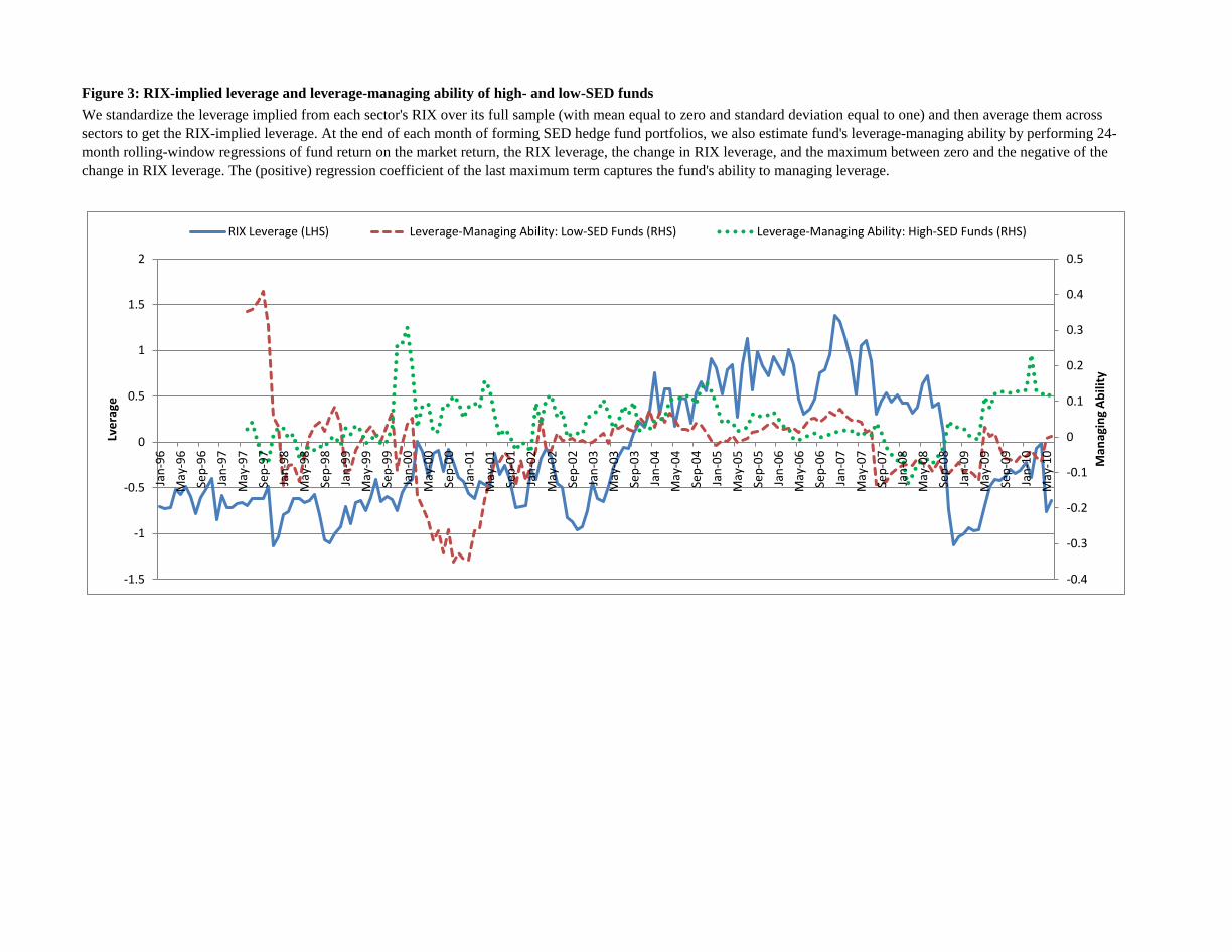
Figure 3: RIX-implied leverage and leverage-managing ability of high- and low-SED fundsWe standardize the leverage implied from each sector's RIX over its full sample (with mean equal to zero and standard deviation equal to one) and then average them across sectors to get the RIX-implied leverage. At the end of each month of forming SED hedge fund portfolios, we also estimate fund's leverage-managing ability by performing 24-month rolling-window regressions of fund return on the market return, the RIX leverage, the change in RIX leverage, and the maximum between zero and the negative of the change in RIX leverage. The (positive) regression coefficient of the last maximum term captures the fund's ability to managing leverage.

-0.4

-0.3

-0.2

-0.1

0

0.1

0.2

0.3

0.4

0.5

-1.5

-1

-0.5

0

0.5

1

1.5

2

Jan-

96M

ay-9

6Se

p-96

Jan-

97M

ay-9

7Se

p-97

Jan-

98M

ay-9

8Se

p-98

Jan-

99M

ay-9

9Se

p-99

Jan-

00M

ay-0

0Se

p-00

Jan-

01M

ay-0

1Se

p-01

Jan-

02M

ay-0

2Se

p-02

Jan-

03M

ay-0

3Se

p-03

Jan-

04M

ay-0

4Se

p-04

Jan-

05M

ay-0

5Se

p-05

Jan-

06M

ay-0

6Se

p-06

Jan-

07M

ay-0

7Se

p-07

Jan-

08M

ay-0

8Se

p-08

Jan-

09M

ay-0

9Se

p-09

Jan-

10M

ay-1

0

Man

agin

g Ab

ility

Lver

age

RIX Leverage (LHS) Leverage-Managing Ability: Low-SED Funds (RHS) Leverage-Managing Ability: High-SED Funds (RHS)

Table IA-9: Distinction from other fund skills

Table IA-11: Additional results of SED portfolios using the CISDM hedge fund database

Table IA-4: Baseline results with full details of estimated FH and NPPR factor loadings

Table IA-6: SED portfolios with vs. without short credit funds (CDS factor included)

Do Hedge Funds Exploit Rare Disaster Concerns?

Internet Appendix: Additional Analyses and Robustness Checks

Table IA-1: Sector-level index put option open interest

Table IA-5: Double-sorted portfolios

Table IA-10: Additional results of SED portfolios using the HFR hedge fund database

Table IA-7: Hedge fund portfolios based on fund's purchasing/selling disaster insuranceTable IA-8: SED portfolios excluding disaster-insurance-purchase funds

Table IA-2: Portfolios independently sorted on SED and conditional tail risk Table IA-3: Portfolios sequentially sorted on conditional tail risk and SED

Table IA-1: Daily open interest of sector-level index put options

K/S ≤ 0.90 0.90 < K/S ≤ 0.95 0.95 < K/S ≤ 1.00 1.00 < K/S ≤ 1.05 1.05 < K/S ≤ 1.10 K/S > 1.10

KBW Banking Sector (BKX) 458 567 930 621 370 180

PHLX Semiconductor Sector (SOX) 131 203 231 178 107 59

PHLX Gold Silver Sector (XAU) 702 1042 900 621 406 221

PHLX Housing Sector (HGX) 272 479 581 444 465 306

PHLX Oil Service Sector (OSX) 636 1209 1562 1326 1005 536

PHLX Utility Sector (UTY) 50 71 116 58 53 85

We select sector-level index put options with 14-60 days of maturity and divided them into six moneyness groups (i.e., K/S, the ratio between strike and underlying index level). Within a moneyness group we first calculate the average of daily open interest (in number of contracts) for each year from 1996 to 2011. The table reports the average of these numbers over years. The following daily options data come from OptionMetrics: BKX (1996/01-2011/12), SOX (1996/01-2011/12), XAU (1996/01-2011/12), HGX (2002/07-2011/12), OSX (1997/02-2011/12), and UTY (1996/01-2011/12). Options must all have non-zero open interest, standard expiration dates, non-missing implied volatility, and valid bid and ask prices (see Section 3.1 in the main text for details about cleaning data).

Table IA-2: Portfolios independently sorted on SED and conditional tail risk

SCTR 1- Low 2 3 4 SCTR 5 -

High SCTR 5 - 1 F-H Alpha

NPPR Alpha

SED 1 - Low 0.042 -0.078 0.101 0.107 -0.091 -0.133 -0.394 -0.247(0.19) (-0.35) (0.45) (0.42) (-0.21) (-0.30) (-1.36) (-0.73)

2 0.446 0.111 0.236 0.220 0.285 -0.161 -0.442 -0.265(3.39) (1.02) (1.69) (1.01) (0.75) (-0.40) (-2.03) (-0.99)

3 0.142 0.201 0.208 0.244 0.289 0.147 -0.023 0.014(1.17) (2.28) (1.67) (1.12) (0.80) (0.42) (-0.13) (0.06)

4 0.349 0.275 0.247 0.217 0.545 0.196 -0.046 0.086(3.35) (3.80) (1.86) (1.11) (1.58) (0.55) (-0.27) (0.37)

SED 5 - High 0.400 0.484 0.524 0.445 0.608 0.208 0.175 -0.020(2.34) (3.29) (2.83) (1.88) (1.59) (0.49) (0.77) (-0.06)

SED 5 - 1 0.358 0.603 0.422 0.337 0.698(1.51) (2.67) (2.21) (2.16) (2.67)

F-H Alpha 0.480 0.746 0.496 0.436 1.050(1.95) (3.38) (2.66) (2.67) (4.21)

NPPR Alpha 0.378 0.597 0.469 0.281 0.605(1.53) (2.68) (2.52) (1.75) (2.29)

ICTR 1- Low 2 3 4 ICTR 5 -

High ICTR 5 - 1 F-H Alpha

NPPR Alpha

SED 1 - Low 0.162 0.029 0.157 -0.026 -0.271 -0.433 -0.329 -0.464(0.55) (0.12) (0.64) (-0.11) (-0.81) (-1.62) (-1.25) (-1.76)

2 0.542 0.281 0.194 0.077 0.190 -0.352 -0.130 -0.415(2.09) (1.86) (1.28) (0.53) (0.73) (-1.23) (-0.46) (-1.49)

3 0.361 0.269 0.134 0.102 0.024 -0.337 -0.249 -0.339(1.43) (1.95) (1.12) (0.77) (0.09) (-1.34) (-0.95) (-1.33)

4 0.512 0.257 0.274 0.311 0.302 -0.214 -0.149 -0.240(2.43) (1.67) (2.48) (2.27) (1.19) (-0.82) (-0.55) (-0.92)

SED 5 - High 0.624 0.662 0.634 0.478 0.584 -0.040 0.124 -0.070(2.65) (3.39) (2.90) (3.00) (2.25) (-0.15) (0.45) (-0.25)

SED 5 - 1 0.462 0.633 0.477 0.503 0.856(2.20) (2.93) (2.12) (2.68) (3.20)

F-H Alpha 0.665 0.821 0.695 0.660 1.118(3.27) (3.90) (3.07) (3.72) (4.79)

NPPR Alpha 0.430 0.598 0.387 0.464 0.824(2.09) (2.77) (1.74) (2.57) (3.35)

Each month, we construct 5x5 hedge fund portfolios by independent sorts on SED and SCTR (the top panel), and on SED and ICTR (the bottom panel). The table presents equal-weighted monthly excess returns as well as F-H and NPPR alphas of long-short hedge portfolios.

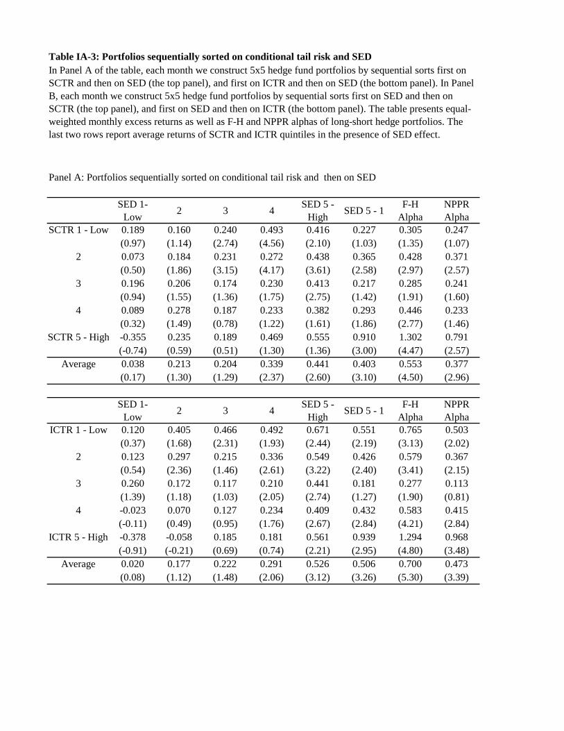
Table IA-3: Portfolios sequentially sorted on conditional tail risk and SED

Panel A: Portfolios sequentially sorted on conditional tail risk and then on SED

SED 1- Low 2 3 4 SED 5 -

High SED 5 - 1 F-H Alpha

NPPR Alpha

SCTR 1 - Low 0.189 0.160 0.240 0.493 0.416 0.227 0.305 0.247(0.97) (1.14) (2.74) (4.56) (2.10) (1.03) (1.35) (1.07)

2 0.073 0.184 0.231 0.272 0.438 0.365 0.428 0.371(0.50) (1.86) (3.15) (4.17) (3.61) (2.58) (2.97) (2.57)

3 0.196 0.206 0.174 0.230 0.413 0.217 0.285 0.241(0.94) (1.55) (1.36) (1.75) (2.75) (1.42) (1.91) (1.60)

4 0.089 0.278 0.187 0.233 0.382 0.293 0.446 0.233(0.32) (1.49) (0.78) (1.22) (1.61) (1.86) (2.77) (1.46)

SCTR 5 - High -0.355 0.235 0.189 0.469 0.555 0.910 1.302 0.791(-0.74) (0.59) (0.51) (1.30) (1.36) (3.00) (4.47) (2.57)

Average 0.038 0.213 0.204 0.339 0.441 0.403 0.553 0.377(0.17) (1.30) (1.29) (2.37) (2.60) (3.10) (4.50) (2.96)

SED 1- Low 2 3 4 SED 5 -

High SED 5 - 1 F-H Alpha

NPPR Alpha

ICTR 1 - Low 0.120 0.405 0.466 0.492 0.671 0.551 0.765 0.503(0.37) (1.68) (2.31) (1.93) (2.44) (2.19) (3.13) (2.02)

2 0.123 0.297 0.215 0.336 0.549 0.426 0.579 0.367(0.54) (2.36) (1.46) (2.61) (3.22) (2.40) (3.41) (2.15)

3 0.260 0.172 0.117 0.210 0.441 0.181 0.277 0.113(1.39) (1.18) (1.03) (2.05) (2.74) (1.27) (1.90) (0.81)

4 -0.023 0.070 0.127 0.234 0.409 0.432 0.583 0.415(-0.11) (0.49) (0.95) (1.76) (2.67) (2.84) (4.21) (2.84)

ICTR 5 - High -0.378 -0.058 0.185 0.181 0.561 0.939 1.294 0.968(-0.91) (-0.21) (0.69) (0.74) (2.21) (2.95) (4.80) (3.48)

Average 0.020 0.177 0.222 0.291 0.526 0.506 0.700 0.473(0.08) (1.12) (1.48) (2.06) (3.12) (3.26) (5.30) (3.39)

In Panel A of the table, each month we construct 5x5 hedge fund portfolios by sequential sorts first on SCTR and then on SED (the top panel), and first on ICTR and then on SED (the bottom panel). In Panel B, each month we construct 5x5 hedge fund portfolios by sequential sorts first on SED and then on SCTR (the top panel), and first on SED and then on ICTR (the bottom panel). The table presents equal-weighted monthly excess returns as well as F-H and NPPR alphas of long-short hedge portfolios. The last two rows report average returns of SCTR and ICTR quintiles in the presence of SED effect.

Panel B: Portfolios sequentially sorted on SED and then conditional tail risk

SCTR 1- Low 2 3 4 SCTR 5 -

High SCTR 5 - 1 F-H Alpha

NPPR Alpha

SED 1 - Low -0.078 -0.035 0.060 -0.385 -0.064 0.014 -0.260 -0.139(-0.37) (-0.16) (0.22) (-1.07) (-0.13) (0.03) (-0.87) (-0.40)

2 0.308 0.127 0.163 0.206 0.300 -0.008 -0.251 -0.081(2.75) (1.11) (1.12) (1.06) (0.87) (-0.02) (-1.35) (-0.36)

3 0.091 0.159 0.170 0.299 0.215 0.124 -0.080 0.043(0.84) (1.58) (1.57) (1.83) (0.74) (0.46) (-0.53) (0.23)

4 0.379 0.284 0.324 0.199 0.498 0.119 -0.089 -0.009(4.02) (3.88) (3.13) (1.29) (1.69) (0.40) (-0.60) (-0.05)

SED 5 - High 0.467 0.624 0.527 0.588 0.749 0.282 0.320 0.038(2.23) (4.39) (2.89) (2.32) (1.80) (0.58) (1.19) (0.10)

Average 0.233 0.232 0.249 0.181 0.340 0.106 -0.072 -0.030(2.17) (2.17) (1.74) (0.87) (0.97) (0.31) (-0.49) (-0.14)

ICTR 1- Low 2 3 4 ICTR 5 -

High ICTR 5 - 1 F-H Alpha

NPPR Alpha

SED 1 - Low 0.138 -0.010 0.006 -0.183 -0.408 -0.546 -0.447 -0.598(0.42) (-0.04) (0.03) (-0.64) (-1.01) (-1.48) (-1.24) (-1.69)

2 0.436 0.210 0.213 0.017 0.228 -0.208 -0.059 -0.294(1.97) (1.23) (1.61) (0.10) (0.94) (-0.84) (-0.24) (-1.23)

3 0.392 0.208 0.140 0.140 0.062 -0.330 -0.269 -0.323(1.92) (1.76) (1.19) (1.28) (0.29) (-1.93) (-1.53) (-1.85)

4 0.464 0.280 0.265 0.306 0.378 -0.086 0.003 -0.112(2.66) (2.59) (2.31) (2.55) (1.98) (-0.45) (0.01) (-0.59)

SED 5 - High 0.840 0.490 0.508 0.570 0.572 -0.268 -0.041 -0.187(2.95) (2.83) (2.75) (3.25) (2.15) (-0.87) (-0.13) (-0.57)

Average 0.454 0.236 0.226 0.170 0.167 -0.288 -0.163 -0.303(2.05) (1.61) (1.65) (1.12) (0.72) (-1.38) (-0.78) (-1.45)

Table IA-4: Factor loadings of SED hedge fund portfolios

Panel A: Fung-Hsieh 8-factor modelExploit Rare

Disaster Concerns

Intercept MKT EMI SMB TERM DEF PTFSBD PTFSFX PTFSCOM

Equal-weighted portfolio returns1 - Low Skill -0.628 0.108 0.451 0.075 0.304 0.247 -0.017 0.011 0.019

(-2.81) (1.01) (7.71) (1.23) (2.05) (1.10) (-0.83) (0.83) (1.22)2 -0.117 0.123 0.222 0.096 0.233 0.325 0.003 -0.000 0.023

(-0.93) (2.07) (7.75) (2.95) (2.43) (2.17) (0.40) (-0.01) (2.59)3 0.008 0.133 0.176 0.075 0.252 0.303 -0.001 0.008 0.014

(0.07) (2.24) (6.09) (2.03) (2.77) (2.15) (-0.07) (1.20) (1.65)4 0.044 0.117 0.144 0.075 0.177 0.225 -0.009 0.006 0.007

(0.37) (2.63) (5.43) (1.87) (2.47) (1.72) (-0.90) (1.09) (0.98)5 -0.001 0.090 0.144 0.095 0.166 0.217 -0.018 0.005 0.003

(-0.01) (2.10) (4.55) (3.05) (2.30) (1.82) (-0.83) (0.72) (0.39)6 0.090 0.108 0.106 0.067 0.114 0.186 -0.009 0.005 0.008

(0.84) (2.95) (4.44) (1.71) (1.71) (1.77) (-0.83) (0.95) (1.08)7 0.150 0.091 0.098 0.092 0.142 0.201 -0.002 0.006 0.003

(1.70) (2.58) (4.66) (1.71) (2.21) (2.26) (-0.30) (1.23) (0.47)8 0.233 0.092 0.108 0.090 0.119 0.193 -0.000 0.007 0.004

(2.56) (2.77) (4.73) (3.79) (1.62) (2.10) (-0.05) (1.30) (0.69)9 0.347 0.230 0.092 0.184 0.052 -0.013 -0.005 0.011 0.016

(2.43) (3.46) (2.73) (2.26) (0.44) (-0.07) (-0.41) (1.01) (1.80)10 - High Skill 0.668 0.127 0.153 0.258 -0.029 -0.043 0.006 0.024 0.018

(3.44) (1.78) (3.00) (2.50) (-0.16) (-0.18) (0.48) (1.66) (1.30)High - Low 1.267 0.026 -0.293 0.230 -0.340 -0.284 0.021 0.019 0.003

(3.78) (0.23) (-3.13) (1.72) (-1.20) (-0.77) (0.68) (0.87) (0.15)

Value-weighted portfolio returns1 - Low Skill -0.701 0.071 0.394 0.054 0.362 0.365 -0.029 0.006 0.027

(-2.25) (0.54) (5.77) (0.64) (1.61) (1.45) (-1.03) (0.35) (1.12)2 -0.272 0.085 0.215 0.225 0.337 0.416 -0.012 -0.007 0.023

(-1.12) (0.88) (4.84) (3.42) (1.55) (1.64) (-0.87) (-0.43) (1.31)3 -0.059 0.161 0.181 0.081 0.304 0.347 -0.017 0.008 0.023

(-0.34) (1.69) (3.72) (1.84) (2.29) (1.83) (-1.05) (0.91) (1.93)4 0.167 0.093 0.114 0.048 0.148 0.234 -0.018 0.007 0.016

(1.15) (1.73) (2.42) (0.95) (1.48) (1.69) (-1.72) (0.99) (1.77)5 -0.049 0.065 0.144 0.127 0.229 0.228 -0.029 0.004 0.004

(-0.26) (1.45) (3.92) (2.80) (2.38) (1.50) (-1.24) (0.56) (0.39)6 0.047 0.081 0.114 0.057 0.160 0.197 -0.019 0.003 0.008

(0.34) (1.83) (4.05) (1.69) (1.85) (1.45) (-1.35) (0.51) (0.94)7 0.210 0.076 0.102 0.130 0.159 0.179 0.001 -0.005 0.011

(1.62) (1.41) (3.50) (1.59) (1.61) (1.17) (0.11) (-0.56) (1.22)8 0.256 0.089 0.090 0.087 0.106 0.153 -0.008 0.005 0.008

(2.12) (2.08) (2.76) (3.72) (1.28) (1.47) (-1.04) (0.70) (1.03)9 0.210 0.285 0.028 0.178 -0.239 0.053 -0.044 0.014 0.019

(0.98) (2.93) (0.63) (1.64) (-1.12) (0.21) (-2.16) (0.93) (1.23)10 - High Skill 0.590 0.014 0.111 0.346 0.041 0.062 -0.010 0.016 0.031

(2.42) (0.15) (1.77) (2.75) (0.24) (0.28) (-0.52) (1.08) (1.50)High - Low 1.224 -0.032 -0.252 0.348 -0.291 -0.325 0.015 0.013 0.015

(3.02) (-0.26) (-2.56) (2.33) (-1.04) (-0.91) (0.39) (0.61) (0.65)

This table reports regression intercepts and factor loadings of monthly formed SED hedge fund deciles in our baseline analysis (see Table 6 in the main text). In Panel A, we use the Fung-Hsieh 8-factor model, including the market factor (MKTRF), the emerging market factor (EMI), the size factor (SMB), the term factor (TERM), the default factor (DEF), and three trend-following factors (PTFSBD, PTFSFX, and PTFSCOM). Following Sadka (2010), TERM and DEF factors are tradable bond portfolio returns based on the 7-10-year Treasury Index and the Corporate Bond Baa Index from Barclays Capital. Note these return-based factors are negatively correlated with term risk and default risk factors used in Table 7 in the main text because of the negative relation between yield and price. In Panel B, we use the Namvar-Phillips-Pukthuanthong-Rau 10-factor model that is constructed using 10 return-based global principal components extracted from 251 assets across various markets and asset classes.

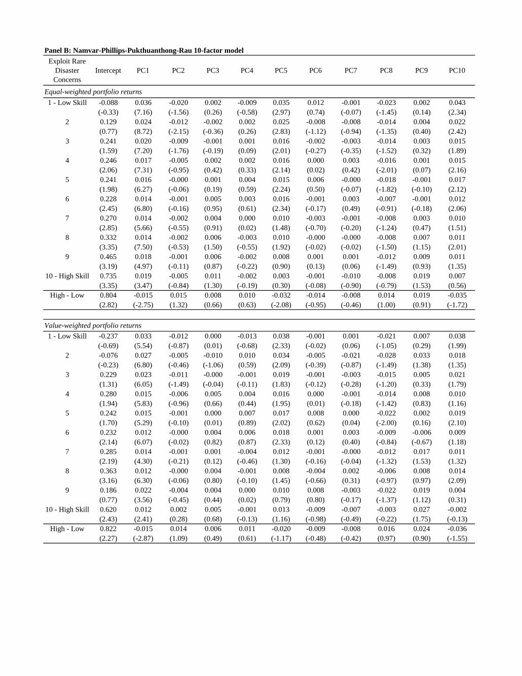
Panel B: Namvar-Phillips-Pukthuanthong-Rau 10-factor modelExploit Rare

Disaster Concerns

Intercept PC1 PC2 PC3 PC4 PC5 PC6 PC7 PC8 PC9 PC10

Equal-weighted portfolio returns1 - Low Skill -0.088 0.036 -0.020 0.002 -0.009 0.035 0.012 -0.001 -0.023 0.002 0.043

(-0.33) (7.16) (-1.56) (0.26) (-0.58) (2.97) (0.74) (-0.07) (-1.45) (0.14) (2.34)2 0.129 0.024 -0.012 -0.002 0.002 0.025 -0.008 -0.008 -0.014 0.004 0.022

(0.77) (8.72) (-2.15) (-0.36) (0.26) (2.83) (-1.12) (-0.94) (-1.35) (0.40) (2.42)3 0.241 0.020 -0.009 -0.001 0.001 0.016 -0.002 -0.003 -0.014 0.003 0.015

(1.59) (7.20) (-1.76) (-0.19) (0.09) (2.01) (-0.27) (-0.35) (-1.52) (0.32) (1.89)4 0.246 0.017 -0.005 0.002 0.002 0.016 0.000 0.003 -0.016 0.001 0.015

(2.06) (7.31) (-0.95) (0.42) (0.33) (2.14) (0.02) (0.42) (-2.01) (0.07) (2.16)5 0.241 0.016 -0.000 0.001 0.004 0.015 0.006 -0.000 -0.018 -0.001 0.017

(1.98) (6.27) (-0.06) (0.19) (0.59) (2.24) (0.50) (-0.07) (-1.82) (-0.10) (2.12)6 0.228 0.014 -0.001 0.005 0.003 0.016 -0.001 0.003 -0.007 -0.001 0.012

(2.45) (6.80) (-0.16) (0.95) (0.61) (2.34) (-0.17) (0.49) (-0.91) (-0.18) (2.06)7 0.270 0.014 -0.002 0.004 0.000 0.010 -0.003 -0.001 -0.008 0.003 0.010

(2.85) (5.66) (-0.55) (0.91) (0.02) (1.48) (-0.70) (-0.20) (-1.24) (0.47) (1.51)8 0.332 0.014 -0.002 0.006 -0.003 0.010 -0.000 -0.000 -0.008 0.007 0.011

(3.35) (7.50) (-0.53) (1.50) (-0.55) (1.92) (-0.02) (-0.02) (-1.50) (1.15) (2.01)9 0.465 0.018 -0.001 0.006 -0.002 0.008 0.001 0.001 -0.012 0.009 0.011

(3.19) (4.97) (-0.11) (0.87) (-0.22) (0.90) (0.13) (0.06) (-1.49) (0.93) (1.35)10 - High Skill 0.735 0.019 -0.005 0.011 -0.002 0.003 -0.001 -0.010 -0.008 0.019 0.007

(3.35) (3.47) (-0.84) (1.30) (-0.19) (0.30) (-0.08) (-0.90) (-0.79) (1.53) (0.56)High - Low 0.804 -0.015 0.015 0.008 0.010 -0.032 -0.014 -0.008 0.014 0.019 -0.035

(2.82) (-2.75) (1.32) (0.66) (0.63) (-2.08) (-0.95) (-0.46) (1.00) (0.91) (-1.72)

Value-weighted portfolio returns1 - Low Skill -0.237 0.033 -0.012 0.000 -0.013 0.038 -0.001 0.001 -0.021 0.007 0.038

(-0.69) (5.54) (-0.87) (0.01) (-0.68) (2.33) (-0.02) (0.06) (-1.05) (0.29) (1.99)2 -0.076 0.027 -0.005 -0.010 0.010 0.034 -0.005 -0.021 -0.028 0.033 0.018

(-0.23) (6.80) (-0.46) (-1.06) (0.59) (2.09) (-0.39) (-0.87) (-1.49) (1.38) (1.35)3 0.229 0.023 -0.011 -0.000 -0.001 0.019 -0.001 -0.003 -0.015 0.005 0.021

(1.31) (6.05) (-1.49) (-0.04) (-0.11) (1.83) (-0.12) (-0.28) (-1.20) (0.33) (1.79)4 0.280 0.015 -0.006 0.005 0.004 0.016 0.000 -0.001 -0.014 0.008 0.010

(1.94) (5.83) (-0.96) (0.66) (0.44) (1.95) (0.01) (-0.18) (-1.42) (0.83) (1.16)5 0.242 0.015 -0.001 0.000 0.007 0.017 0.008 0.000 -0.022 0.002 0.019

(1.70) (5.29) (-0.10) (0.01) (0.89) (2.02) (0.62) (0.04) (-2.00) (0.16) (2.10)6 0.232 0.012 -0.000 0.004 0.006 0.018 0.001 0.003 -0.009 -0.006 0.009

(2.14) (6.07) (-0.02) (0.82) (0.87) (2.33) (0.12) (0.40) (-0.84) (-0.67) (1.18)7 0.285 0.014 -0.001 0.001 -0.004 0.012 -0.001 -0.000 -0.012 0.017 0.011

(2.19) (4.30) (-0.21) (0.12) (-0.46) (1.30) (-0.16) (-0.04) (-1.32) (1.53) (1.32)8 0.363 0.012 -0.000 0.004 -0.001 0.008 -0.004 0.002 -0.006 0.008 0.014

(3.16) (6.30) (-0.06) (0.80) (-0.10) (1.45) (-0.66) (0.31) (-0.97) (0.97) (2.09)9 0.186 0.022 -0.004 0.004 0.000 0.010 0.008 -0.003 -0.022 0.019 0.004

(0.77) (3.56) (-0.45) (0.44) (0.02) (0.79) (0.80) (-0.17) (-1.37) (1.12) (0.31)10 - High Skill 0.620 0.012 0.002 0.005 -0.001 0.013 -0.009 -0.007 -0.003 0.027 -0.002

(2.43) (2.41) (0.28) (0.68) (-0.13) (1.16) (-0.98) (-0.49) (-0.22) (1.75) (-0.13)High - Low 0.822 -0.015 0.014 0.006 0.011 -0.020 -0.009 -0.008 0.016 0.024 -0.036

(2.27) (-2.87) (1.09) (0.49) (0.61) (-1.17) (-0.48) (-0.42) (0.97) (0.90) (-1.55)

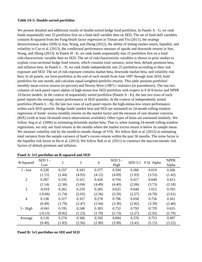
Table IA-5: Double-sorted portfolios

Panel A: 5×5 portfolios on R-squared and SED

R-Squared SED 1 - Low 2 3 4 SED 5 -

High SED 5-1 F-H Alpha NPPR Alpha

1 - low 0.228 0.257 0.343 0.377 0.594 0.366 0.619 0.266(1.15) (2.44) (4.93) (4.12) (4.09) (1.93) (3.53) (1.42)

2 0.287 0.335 0.321 0.426 0.704 0.417 0.649 0.413(1.14) (2.36) (3.04) (4.49) (4.40) (2.06) (3.73) (2.18)

3 -0.019 0.265 0.259 0.285 0.625 0.644 1.012 0.593(-0.06) (1.74) (2.05) (2.36) (3.59) (2.57) (4.78) (2.61)

4 0.138 0.317 0.357 0.278 0.796 0.658 0.756 0.561(0.49) (1.79) (2.47) (1.94) (3.30) (2.82) (3.39) (2.40)

5 - High -0.041 0.195 0.248 0.383 0.752 0.793 0.729 0.655(-0.13) (0.82) (1.23) (1.78) (2.73) (3.27) (2.92) (2.70)

Average 0.118 0.274 0.306 0.350 0.694 0.576 0.753 0.497(0.49) (1.83) (2.56) (2.90) (3.98) (3.41) (5.15) (3.22)

Panel B: 5×5 portfolios on SDI and SED

We present detailed and additional results of double-sorted hedge fund portfolios. In Panels A - G, we rank funds sequentially into 25 portfolios first on a fund skill variable then on SED. The set of fund skill variables contains R-squared from the Fung-Hsieh factor regression in Titman and Tiu (2011), the strategy distinctiveness index (SDI) in Sun, Wang, and Zheng (2012), the ability of timing market return, liquidity, and volatility in Cao et al. (2013), the conditional performance measure of upside and downside returns in Sun, Wang, and Zheng (2013). In Panels H - K, we rank funds sequentially into 25 portfolios first on a fund risk/characteristic variable then on SED. The set of risk/characteristic variables is shown in prior studies to explain cross-sectional hedge fund returns, which contains total variance, noise beta, default premium beta, and inflation beta. In Panels L - N, we rank funds independently into 25 portfolios according to their risk exposure and SED. The set of risk exposure contains market beta, downside market beta, and volatility risk beta. In all panels, we form portfolios at the end of each month from June 1997 through June 2010, hold portfolios for one month, and calculate equal-weighted portfolio returns. This table presents portfolios’ monthly mean excess returns (in percent) and Newey-West (1987) t -statistics (in parentheses). The last two columns of each panel report alphas of high-minus-low SED portfolios with respect to F-H 8-factor and NPPR 10-factor models. In the context of sequentially sorted portfolios (Panels A - K), the last two rows of each panel reports the average return performance of SED quintiles. In the context of independently sorted portfolios (Panels L - N), the last two rows of each panel reports the high-minus-low return performance within each SED quintile. Hedge funds' market beta and SED are estimated on 24-month rolling-window regression of funds’ excess monthly returns on the market factor and the measure of rare disaster concerns (RIX) (with at least 18-month return observations available). Other types of betas are estimated similarly. We follow Ang et al. (2006) in estimating downside market beta. That is, when running 24-month rolling-window regressions, we only use fund returns in the months where the market excess return is below its sample mean. We measure volatility risk by the month-to-month change of VIX. We follow Bali et al. (2012) in estimating total variance from the sample variance of fund’s excess returns within the past 36 months. The noise factor is the liquidity risk factor in Hu et al. (2013). We follow Bali et al. (2011) to construct the macroeconomic risk factors of default premium and inflation.

SDI SED 1 - Low 2 3 4 SED 5 -

High SED 5-1 F-H Alpha NPPR Alpha

1 - low -0.480 0.097 0.220 0.525 0.884 1.364 1.656 1.156(-1.10) (0.36) (0.88) (2.29) (3.06) (3.68) (4.98) (3.45)

2 0.158 0.350 0.330 0.502 0.903 0.745 0.799 0.674(0.52) (1.55) (1.72) (2.79) (3.47) (3.21) (3.53) (2.89)

3 0.399 0.342 0.391 0.435 0.752 0.353 0.534 0.302(1.57) (2.02) (2.49) (3.12) (3.36) (1.73) (2.78) (1.45)

4 0.254 0.363 0.365 0.444 0.750 0.496 0.602 0.521(1.36) (3.33) (4.73) (4.30) (4.13) (2.64) (3.20) (2.64)

5 - High 0.359 0.284 0.341 0.251 0.596 0.236 0.374 0.184(2.95) (3.67) (7.14) (3.55) (6.21) (1.87) (3.07) (1.46)

Average 0.138 0.287 0.329 0.431 0.777 0.639 0.793 0.568(0.59) (1.85) (2.47) (3.34) (4.20) (3.83) (5.26) (3.56)

Panel C: 5×5 sequential portfolios on market-timing ability and SEDTiming (Market Return)

SED 1 - Low 2 3 4 SED 5 -

High SED 5-1 F-H Alpha NPPR Alpha

1 - low 0.010 0.307 0.400 0.522 0.912 0.903 1.232 0.928(0.03) (1.54) (2.16) (2.54) (3.85) (3.88) (5.89) (4.16)

2 0.228 0.333 0.314 0.317 0.578 0.349 0.480 0.359(1.07) (2.31) (2.59) (2.44) (3.90) (2.37) (3.64) (2.72)

3 0.277 0.252 0.264 0.280 0.489 0.212 0.251 0.194(1.41) (1.92) (2.37) (2.74) (3.00) (1.76) (2.06) (1.62)

4 0.126 0.150 0.151 0.373 0.528 0.402 0.594 0.409(0.50) (0.83) (0.92) (2.84) (3.19) (2.58) (4.40) (3.10)

5 - High 0.009 0.115 0.404 0.437 0.829 0.821 1.241 0.680(0.02) (0.39) (1.88) (1.89) (2.82) (2.64) (4.56) (2.46)

Average 0.130 0.231 0.306 0.386 0.667 0.537 0.760 0.514(0.50) (1.30) (2.07) (2.59) (3.64) (3.37) (5.59) (3.75)

Panel D: 5×5 portfolios on liquidity-timing ability and SEDTiming (Market

Liquidity)

SED 1 - Low 2 3 4 SED 5 -

High SED 5-1 F-H Alpha NPPR Alpha

1 - low 0.099 0.095 0.401 0.472 0.818 0.719 1.143 0.585(0.23) (0.35) (1.67) (2.04) (2.78) (2.51) (4.32) (2.29)

2 0.141 0.245 0.158 0.248 0.443 0.303 0.412 0.321(0.65) (1.67) (1.12) (1.88) (2.57) (2.37) (3.30) (2.58)

3 0.229 0.249 0.220 0.255 0.493 0.263 0.460 0.205(1.05) (1.61) (1.83) (2.42) (3.19) (1.84) (3.56) (1.74)

4 0.094 0.352 0.363 0.351 0.635 0.541 0.638 0.494(0.45) (2.44) (2.76) (2.94) (3.66) (3.55) (4.34) (3.44)

5 - High 0.047 0.300 0.376 0.639 0.867 0.820 1.124 0.817(0.15) (1.41) (1.83) (3.37) (3.59) (3.25) (4.68) (3.42)

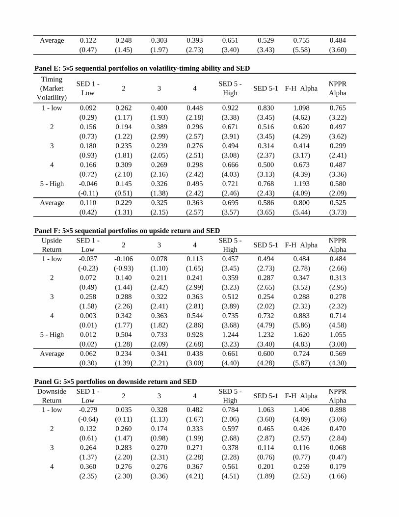
Average 0.122 0.248 0.303 0.393 0.651 0.529 0.755 0.484(0.47) (1.45) (1.97) (2.73) (3.40) (3.43) (5.58) (3.60)

Panel E: 5×5 sequential portfolios on volatility-timing ability and SEDTiming (Market

Volatility)

SED 1 - Low 2 3 4 SED 5 -

High SED 5-1 F-H Alpha NPPR Alpha

1 - low 0.092 0.262 0.400 0.448 0.922 0.830 1.098 0.765(0.29) (1.17) (1.93) (2.18) (3.38) (3.45) (4.62) (3.22)

2 0.156 0.194 0.389 0.296 0.671 0.516 0.620 0.497(0.73) (1.22) (2.99) (2.57) (3.91) (3.45) (4.29) (3.62)

3 0.180 0.235 0.239 0.276 0.494 0.314 0.414 0.299(0.93) (1.81) (2.05) (2.51) (3.08) (2.37) (3.17) (2.41)

4 0.166 0.309 0.269 0.298 0.666 0.500 0.673 0.487(0.72) (2.10) (2.16) (2.42) (4.03) (3.13) (4.39) (3.36)

5 - High -0.046 0.145 0.326 0.495 0.721 0.768 1.193 0.580(-0.11) (0.51) (1.38) (2.42) (2.46) (2.43) (4.09) (2.09)

Average 0.110 0.229 0.325 0.363 0.695 0.586 0.800 0.525(0.42) (1.31) (2.15) (2.57) (3.57) (3.65) (5.44) (3.73)

Panel F: 5×5 sequential portfolios on upside return and SEDUpside Return

SED 1 - Low 2 3 4 SED 5 -

High SED 5-1 F-H Alpha NPPR Alpha

1 - low -0.037 -0.106 0.078 0.113 0.457 0.494 0.484 0.484(-0.23) (-0.93) (1.10) (1.65) (3.45) (2.73) (2.78) (2.66)

2 0.072 0.140 0.211 0.241 0.359 0.287 0.347 0.313(0.49) (1.44) (2.42) (2.99) (3.23) (2.65) (3.52) (2.95)

3 0.258 0.288 0.322 0.363 0.512 0.254 0.288 0.278(1.58) (2.26) (2.41) (2.81) (3.89) (2.02) (2.32) (2.32)

4 0.003 0.342 0.363 0.544 0.735 0.732 0.883 0.714(0.01) (1.77) (1.82) (2.86) (3.68) (4.79) (5.86) (4.58)

5 - High 0.012 0.504 0.733 0.928 1.244 1.232 1.620 1.055(0.02) (1.28) (2.09) (2.68) (3.23) (3.40) (4.83) (3.08)

Average 0.062 0.234 0.341 0.438 0.661 0.600 0.724 0.569(0.30) (1.39) (2.21) (3.00) (4.40) (4.28) (5.87) (4.30)

Panel G: 5×5 portfolios on downside return and SEDDownside

ReturnSED 1 -

Low 2 3 4 SED 5 - High SED 5-1 F-H Alpha NPPR

Alpha1 - low -0.279 0.035 0.328 0.482 0.784 1.063 1.406 0.898

(-0.64) (0.11) (1.13) (1.67) (2.06) (3.60) (4.89) (3.06)2 0.132 0.260 0.174 0.333 0.597 0.465 0.426 0.470

(0.61) (1.47) (0.98) (1.99) (2.68) (2.87) (2.57) (2.84)3 0.264 0.283 0.270 0.271 0.378 0.114 0.116 0.068

(1.37) (2.20) (2.31) (2.28) (2.28) (0.76) (0.77) (0.47)4 0.360 0.276 0.276 0.367 0.561 0.201 0.259 0.179

(2.35) (2.30) (3.36) (4.21) (4.51) (1.89) (2.52) (1.66)

5 - High 0.371 0.332 0.411 0.449 0.777 0.406 0.474 0.414(2.06) (2.87) (4.94) (4.28) (4.45) (2.01) (2.32) (2.01)

Average 0.170 0.237 0.292 0.381 0.620 0.450 0.536 0.406(0.83) (1.57) (2.19) (2.85) (3.53) (3.41) (4.16) (3.07)

Panel H: 5×5 sequential portfolios on total variance and SEDTotal

VarianceSED 1 -

Low 2 3 4 SED 5 - High SED 5-1 F-H Alpha NPPR

Alpha1 - low 0.113 0.198 0.226 0.271 0.281 0.168 0.245 0.179

(1.21) (2.69) (3.49) (5.71) (4.93) (2.33) (3.66) (2.50)2 0.206 0.212 0.227 0.207 0.405 0.199 0.207 0.260

(1.76) (1.78) (2.02) (2.03) (4.74) (2.14) (2.22) (2.84)3 0.323 0.317 0.313 0.364 0.490 0.167 0.207 0.179

(2.20) (1.97) (2.06) (2.65) (4.32) (1.55) (1.88) (1.69)4 0.161 0.229 0.394 0.565 0.737 0.576 0.601 0.578

(0.80) (1.16) (2.01) (2.83) (4.25) (3.29) (3.61) (3.29)5 - High -0.113 0.162 0.527 0.760 1.144 1.257 1.673 1.065

(-0.26) (0.44) (1.49) (2.29) (3.81) (3.39) (5.21) (3.22)Average 0.138 0.224 0.338 0.433 0.612 0.474 0.587 0.452

(0.75) (1.31) (2.04) (2.83) (4.82) (3.64) (5.05) (3.71)

Panel I: 5×5 sequential portfolios on noise beta and SED

Noise Beta SED 1 - Low 2 3 4 SED 5 -

High SED 5-1 F-H Alpha NPPR Alpha

1 - low 0.497 0.500 0.633 0.946 1.111 0.614 0.677 0.485(1.50) (2.08) (2.65) (3.74) (3.85) (2.36) (2.61) (1.86)

2 0.172 0.341 0.311 0.428 0.611 0.439 0.479 0.375(0.90) (2.34) (2.25) (3.22) (3.50) (2.78) (3.11) (2.36)

3 0.174 0.292 0.248 0.298 0.574 0.400 0.480 0.381(0.96) (2.30) (2.31) (3.06) (4.27) (3.05) (3.76) (2.90)

4 -0.041 0.157 0.218 0.326 0.445 0.486 0.622 0.396(-0.20) (1.25) (2.18) (3.54) (3.36) (3.09) (4.39) (2.81)

5 - High -0.437 -0.086 0.111 0.372 0.520 0.957 1.393 0.844(-1.28) (-0.49) (0.69) (2.47) (2.86) (3.19) (5.77) (3.27)

Average 0.073 0.241 0.304 0.474 0.652 0.579 0.730 0.496(0.32) (1.61) (2.25) (3.70) (3.99) (3.60) (5.12) (3.38)

Panel J: 5×5 sequentail portfolios on default premium beta and SEDDefault

BetaSED 1 -

Low 2 3 4 SED 5 - High SED 5-1 F-H Alpha NPPR

Alpha1 - low -0.307 0.022 0.255 0.290 0.490 0.797 1.000 0.678

(-0.97) (0.10) (1.36) (1.63) (2.12) (2.84) (3.99) (2.62)2 0.003 0.132 0.189 0.302 0.455 0.452 0.558 0.438

(0.01) (0.88) (1.59) (3.05) (3.19) (2.95) (3.89) (3.07)3 0.148 0.212 0.255 0.296 0.498 0.349 0.404 0.338

(0.87) (1.68) (2.51) (3.19) (3.95) (2.83) (3.33) (2.79)4 0.256 0.355 0.274 0.455 0.674 0.418 0.573 0.389

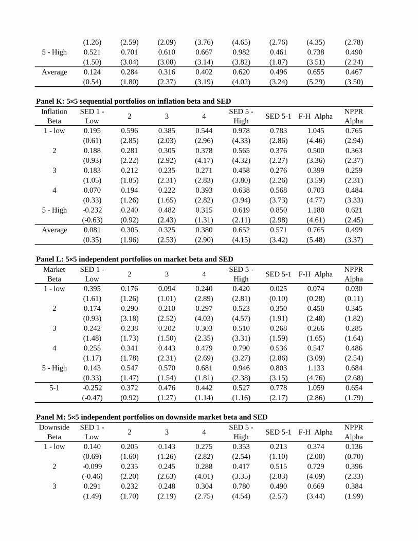
(1.26) (2.59) (2.09) (3.76) (4.65) (2.76) (4.35) (2.78)5 - High 0.521 0.701 0.610 0.667 0.982 0.461 0.738 0.490

(1.50) (3.04) (3.08) (3.14) (3.82) (1.87) (3.51) (2.24)Average 0.124 0.284 0.316 0.402 0.620 0.496 0.655 0.467

(0.54) (1.80) (2.37) (3.19) (4.02) (3.24) (5.29) (3.50)

Panel K: 5×5 sequential portfolios on inflation beta and SEDInflation

BetaSED 1 -

Low 2 3 4 SED 5 - High SED 5-1 F-H Alpha NPPR

Alpha1 - low 0.195 0.596 0.385 0.544 0.978 0.783 1.045 0.765

(0.61) (2.85) (2.03) (2.96) (4.33) (2.86) (4.46) (2.94)2 0.188 0.281 0.305 0.378 0.565 0.376 0.500 0.363

(0.93) (2.22) (2.92) (4.17) (4.32) (2.27) (3.36) (2.37)3 0.183 0.212 0.235 0.271 0.458 0.276 0.399 0.259

(1.05) (1.85) (2.31) (2.83) (3.80) (2.26) (3.59) (2.31)4 0.070 0.194 0.222 0.393 0.638 0.568 0.703 0.484

(0.33) (1.26) (1.65) (2.82) (3.94) (3.73) (4.77) (3.33)5 - High -0.232 0.240 0.482 0.315 0.619 0.850 1.180 0.621

(-0.63) (0.92) (2.43) (1.31) (2.11) (2.98) (4.61) (2.45)Average 0.081 0.305 0.325 0.380 0.652 0.571 0.765 0.499

(0.35) (1.96) (2.53) (2.90) (4.15) (3.42) (5.48) (3.37)

Panel L: 5×5 independent portfolios on market beta and SEDMarket

BetaSED 1 -

Low 2 3 4 SED 5 - High SED 5-1 F-H Alpha NPPR

Alpha1 - low 0.395 0.176 0.094 0.240 0.420 0.025 0.074 0.030

(1.61) (1.26) (1.01) (2.89) (2.81) (0.10) (0.28) (0.11)2 0.174 0.290 0.210 0.297 0.523 0.350 0.450 0.345

(0.93) (3.18) (2.52) (4.03) (4.57) (1.91) (2.48) (1.82)3 0.242 0.238 0.202 0.303 0.510 0.268 0.266 0.285

(1.48) (1.73) (1.50) (2.35) (3.31) (1.59) (1.65) (1.64)4 0.255 0.341 0.443 0.479 0.790 0.536 0.547 0.486

(1.17) (1.78) (2.31) (2.69) (3.27) (2.86) (3.09) (2.54)5 - High 0.143 0.547 0.570 0.681 0.946 0.803 1.133 0.684

(0.33) (1.47) (1.54) (1.81) (2.38) (3.15) (4.76) (2.68)5-1 -0.252 0.372 0.476 0.442 0.527 0.778 1.059 0.654

(-0.47) (0.92) (1.27) (1.14) (1.16) (2.17) (2.86) (1.79)

Panel M: 5×5 independent portfolios on downside market beta and SEDDownside

BetaSED 1 -

Low 2 3 4 SED 5 - High SED 5-1 F-H Alpha NPPR

Alpha1 - low 0.140 0.205 0.143 0.275 0.353 0.213 0.374 0.136

(0.69) (1.60) (1.26) (2.82) (2.54) (1.10) (2.00) (0.70)2 -0.099 0.235 0.245 0.288 0.417 0.515 0.729 0.396

(-0.46) (2.20) (2.63) (4.01) (3.35) (2.83) (4.09) (2.33)3 0.291 0.232 0.248 0.304 0.780 0.490 0.669 0.384

(1.49) (1.70) (2.19) (2.75) (4.54) (2.57) (3.44) (1.99)

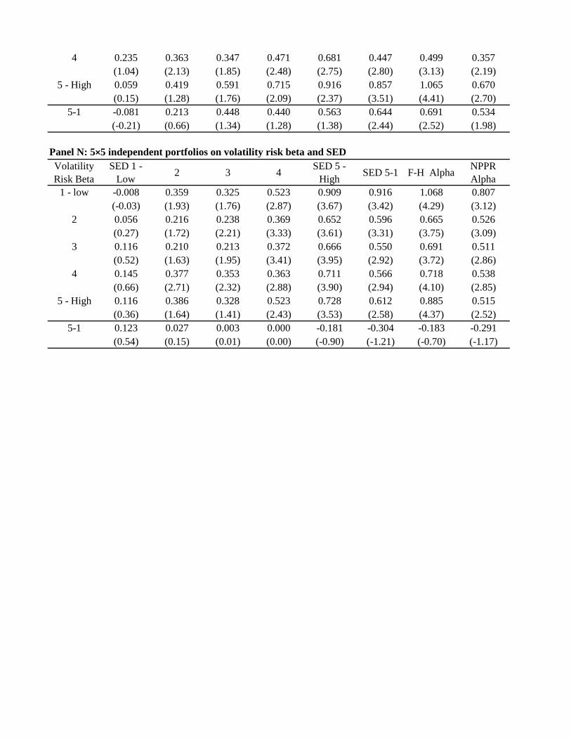
4 0.235 0.363 0.347 0.471 0.681 0.447 0.499 0.357(1.04) (2.13) (1.85) (2.48) (2.75) (2.80) (3.13) (2.19)

5 - High 0.059 0.419 0.591 0.715 0.916 0.857 1.065 0.670(0.15) (1.28) (1.76) (2.09) (2.37) (3.51) (4.41) (2.70)

5-1 -0.081 0.213 0.448 0.440 0.563 0.644 0.691 0.534(-0.21) (0.66) (1.34) (1.28) (1.38) (2.44) (2.52) (1.98)

Panel N: 5×5 independent portfolios on volatility risk beta and SEDVolatility Risk Beta

SED 1 - Low 2 3 4 SED 5 -

High SED 5-1 F-H Alpha NPPR Alpha

1 - low -0.008 0.359 0.325 0.523 0.909 0.916 1.068 0.807(-0.03) (1.93) (1.76) (2.87) (3.67) (3.42) (4.29) (3.12)

2 0.056 0.216 0.238 0.369 0.652 0.596 0.665 0.526(0.27) (1.72) (2.21) (3.33) (3.61) (3.31) (3.75) (3.09)

3 0.116 0.210 0.213 0.372 0.666 0.550 0.691 0.511(0.52) (1.63) (1.95) (3.41) (3.95) (2.92) (3.72) (2.86)

4 0.145 0.377 0.353 0.363 0.711 0.566 0.718 0.538(0.66) (2.71) (2.32) (2.88) (3.90) (2.94) (4.10) (2.85)

5 - High 0.116 0.386 0.328 0.523 0.728 0.612 0.885 0.515(0.36) (1.64) (1.41) (2.43) (3.53) (2.58) (4.37) (2.52)

5-1 0.123 0.027 0.003 0.000 -0.181 -0.304 -0.183 -0.291(0.54) (0.15) (0.01) (0.00) (-0.90) (-1.21) (-0.70) (-1.17)

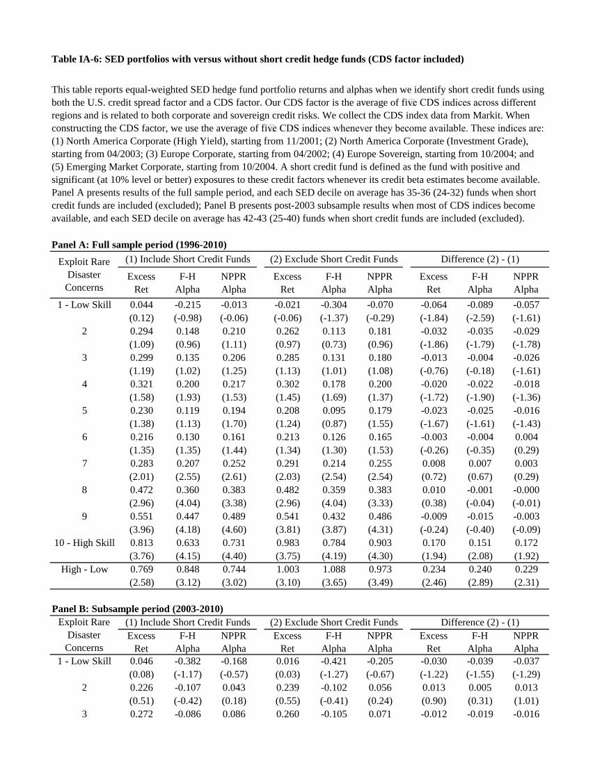
Table IA-6: SED portfolios with versus without short credit hedge funds (CDS factor included)

Panel A: Full sample period (1996-2010)

Excess Ret

F-H Alpha

NPPR Alpha

Excess Ret

F-H Alpha

NPPR Alpha

Excess Ret

F-H Alpha

NPPR Alpha

1 - Low Skill 0.044 -0.215 -0.013 -0.021 -0.304 -0.070 -0.064 -0.089 -0.057(0.12) (-0.98) (-0.06) (-0.06) (-1.37) (-0.29) (-1.84) (-2.59) (-1.61)

2 0.294 0.148 0.210 0.262 0.113 0.181 -0.032 -0.035 -0.029(1.09) (0.96) (1.11) (0.97) (0.73) (0.96) (-1.86) (-1.79) (-1.78)

3 0.299 0.135 0.206 0.285 0.131 0.180 -0.013 -0.004 -0.026(1.19) (1.02) (1.25) (1.13) (1.01) (1.08) (-0.76) (-0.18) (-1.61)

4 0.321 0.200 0.217 0.302 0.178 0.200 -0.020 -0.022 -0.018(1.58) (1.93) (1.53) (1.45) (1.69) (1.37) (-1.72) (-1.90) (-1.36)

5 0.230 0.119 0.194 0.208 0.095 0.179 -0.023 -0.025 -0.016(1.38) (1.13) (1.70) (1.24) (0.87) (1.55) (-1.67) (-1.61) (-1.43)

6 0.216 0.130 0.161 0.213 0.126 0.165 -0.003 -0.004 0.004(1.35) (1.35) (1.44) (1.34) (1.30) (1.53) (-0.26) (-0.35) (0.29)

7 0.283 0.207 0.252 0.291 0.214 0.255 0.008 0.007 0.003(2.01) (2.55) (2.61) (2.03) (2.54) (2.54) (0.72) (0.67) (0.29)

8 0.472 0.360 0.383 0.482 0.359 0.383 0.010 -0.001 -0.000(2.96) (4.04) (3.38) (2.96) (4.04) (3.33) (0.38) (-0.04) (-0.01)

9 0.551 0.447 0.489 0.541 0.432 0.486 -0.009 -0.015 -0.003(3.96) (4.18) (4.60) (3.81) (3.87) (4.31) (-0.24) (-0.40) (-0.09)

10 - High Skill 0.813 0.633 0.731 0.983 0.784 0.903 0.170 0.151 0.172(3.76) (4.15) (4.40) (3.75) (4.19) (4.30) (1.94) (2.08) (1.92)

High - Low 0.769 0.848 0.744 1.003 1.088 0.973 0.234 0.240 0.229(2.58) (3.12) (3.02) (3.10) (3.65) (3.49) (2.46) (2.89) (2.31)

Panel B: Subsample period (2003-2010)

Excess Ret

F-H Alpha

NPPR Alpha

Excess Ret

F-H Alpha

NPPR Alpha

Excess Ret

F-H Alpha

NPPR Alpha

1 - Low Skill 0.046 -0.382 -0.168 0.016 -0.421 -0.205 -0.030 -0.039 -0.037(0.08) (-1.17) (-0.57) (0.03) (-1.27) (-0.67) (-1.22) (-1.55) (-1.29)

2 0.226 -0.107 0.043 0.239 -0.102 0.056 0.013 0.005 0.013(0.51) (-0.42) (0.18) (0.55) (-0.41) (0.24) (0.90) (0.31) (1.01)

3 0.272 -0.086 0.086 0.260 -0.105 0.071 -0.012 -0.019 -0.016

This table reports equal-weighted SED hedge fund portfolio returns and alphas when we identify short credit funds using both the U.S. credit spread factor and a CDS factor. Our CDS factor is the average of fi�ve CDS indices across different regions and is related to both corporate and sovereign credit risks. We collect the CDS index data from Markit. When constructing the CDS factor, we use the average of fi�ve CDS indices whenever they become available. These indices are: (1) North America Corporate (High Yield), starting from 11/2001; (2) North America Corporate (Investment Grade), starting from 04/2003; (3) Europe Corporate, starting from 04/2002; (4) Europe Sovereign, starting from 10/2004; and (5) Emerging Market Corporate, starting from 10/2004. A short credit fund is defined as the fund with positive and significant (at 10% level or better) exposures to these credit factors whenever its credit beta estimates become available. Panel A presents results of the full sample period, and each SED decile on average has 35-36 (24-32) funds when short credit funds are included (excluded); Panel B presents post-2003 subsample results when most of CDS indices become available, and each SED decile on average has 42-43 (25-40) funds when short credit funds are included (excluded).

Exploit Rare Disaster Concerns

(1) Include Short Credit Funds (2) Exclude Short Credit Funds Difference (2) - (1)

Exploit Rare Disaster Concerns

(1) Include Short Credit Funds (2) Exclude Short Credit Funds Difference (2) - (1)

(0.66) (-0.41) (0.39) (0.63) (-0.50) (0.31) (-1.20) (-1.61) (-1.52)4 0.216 -0.100 0.020 0.204 -0.105 0.007 -0.012 -0.005 -0.013

(0.63) (-0.71) (0.11) (0.59) (-0.75) (0.04) (-1.54) (-0.64) (-1.54)5 0.122 -0.188 0.028 0.102 -0.196 0.021 -0.019 -0.008 -0.007

(0.44) (-1.20) (0.21) (0.37) (-1.24) (0.16) (-1.48) (-0.58) (-0.73)6 0.167 -0.074 0.054 0.154 -0.082 0.049 -0.013 -0.008 -0.005

(0.62) (-0.42) (0.39) (0.57) (-0.46) (0.35) (-0.93) (-0.54) (-0.41)7 0.179 -0.085 0.094 0.168 -0.106 0.075 -0.011 -0.021 -0.020

(0.77) (-0.66) (0.79) (0.71) (-0.82) (0.59) (-0.65) (-1.28) (-1.13)8 0.458 0.361 0.292 0.489 0.364 0.297 0.030 0.002 0.005

(1.75) (3.05) (1.70) (1.81) (2.96) (1.72) (0.71) (0.06) (0.19)9 0.530 0.443 0.349 0.570 0.518 0.410 0.040 0.074 0.061

(2.68) (2.78) (2.77) (2.75) (2.82) (2.95) (0.65) (1.52) (1.27)10 - High Skill 0.902 0.717 0.761 1.194 1.002 1.038 0.292 0.285 0.277

(3.20) (3.62) (3.91) (3.32) (3.78) (4.20) (1.94) (2.50) (2.17)High - Low 0.856 1.099 0.928 1.178 1.422 1.243 0.322 0.324 0.314

(1.79) (2.48) (2.86) (2.34) (2.98) (3.27) (2.11) (2.79) (2.41)

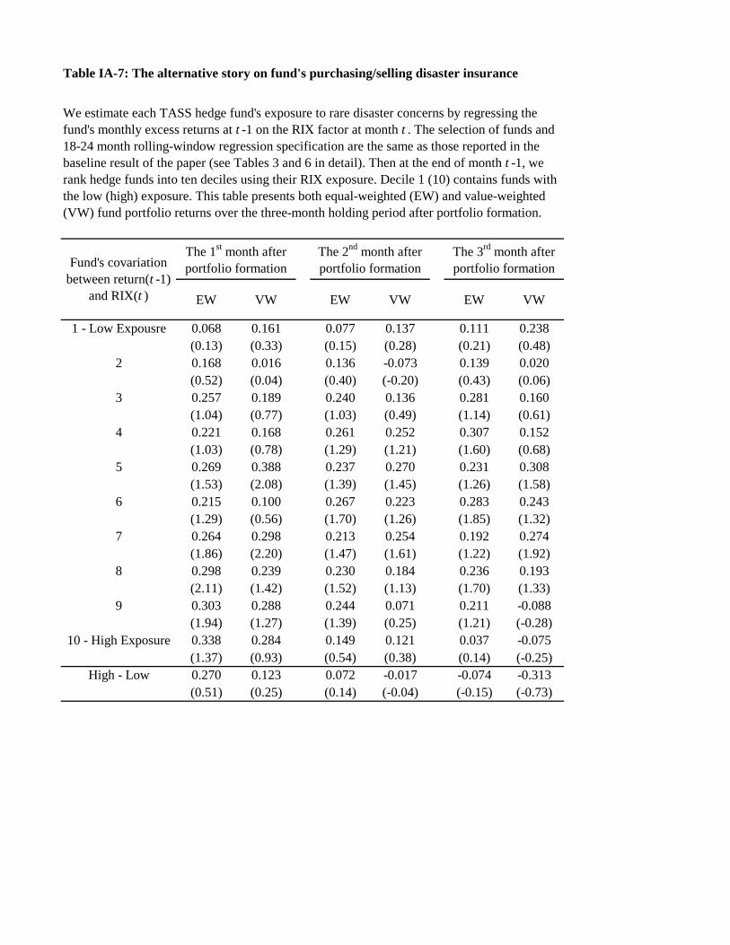
Table IA-7: The alternative story on fund's purchasing/selling disaster insurance

EW VW EW VW EW VW

1 - Low Expousre 0.068 0.161 0.077 0.137 0.111 0.238(0.13) (0.33) (0.15) (0.28) (0.21) (0.48)

2 0.168 0.016 0.136 -0.073 0.139 0.020(0.52) (0.04) (0.40) (-0.20) (0.43) (0.06)

3 0.257 0.189 0.240 0.136 0.281 0.160(1.04) (0.77) (1.03) (0.49) (1.14) (0.61)

4 0.221 0.168 0.261 0.252 0.307 0.152(1.03) (0.78) (1.29) (1.21) (1.60) (0.68)

5 0.269 0.388 0.237 0.270 0.231 0.308(1.53) (2.08) (1.39) (1.45) (1.26) (1.58)

6 0.215 0.100 0.267 0.223 0.283 0.243(1.29) (0.56) (1.70) (1.26) (1.85) (1.32)

7 0.264 0.298 0.213 0.254 0.192 0.274(1.86) (2.20) (1.47) (1.61) (1.22) (1.92)

8 0.298 0.239 0.230 0.184 0.236 0.193(2.11) (1.42) (1.52) (1.13) (1.70) (1.33)

9 0.303 0.288 0.244 0.071 0.211 -0.088(1.94) (1.27) (1.39) (0.25) (1.21) (-0.28)

10 - High Exposure 0.338 0.284 0.149 0.121 0.037 -0.075(1.37) (0.93) (0.54) (0.38) (0.14) (-0.25)

High - Low 0.270 0.123 0.072 -0.017 -0.074 -0.313(0.51) (0.25) (0.14) (-0.04) (-0.15) (-0.73)

The 1st month after portfolio formation

The 2nd month after portfolio formation

The 3rd month after portfolio formationFund's covariation

between return(t -1) and RIX(t )

We estimate each TASS hedge fund's exposure to rare disaster concerns by regressing the fund's monthly excess returns at t -1 on the RIX factor at month t . The selection of funds and 18-24 month rolling-window regression specification are the same as those reported in the baseline result of the paper (see Tables 3 and 6 in detail). Then at the end of month t -1, we rank hedge funds into ten deciles using their RIX exposure. Decile 1 (10) contains funds with the low (high) exposure. This table presents both equal-weighted (EW) and value-weighted (VW) fund portfolio returns over the three-month holding period after portfolio formation.

Table IA-8: SED portfolios excluding disaster-insurance-purchase funds

Excess Ret

F-H Alpha

NPPR Alpha

Excess Ret

F-H Alpha

NPPR Alpha

1 - Low Skill -0.127 -0.576 -0.066 0.077 -0.379 0.062(-0.40) (-2.64) (-0.33) (0.22) (-1.36) (0.26)

2 0.184 -0.026 0.136 -0.004 -0.366 -0.119(0.94) (-0.19) (0.96) (-0.01) (-1.61) (-0.49)

3 0.311 0.103 0.304 0.385 0.180 0.409(1.80) (0.98) (2.84) (2.08) (1.16) (3.26)

4 0.334 0.165 0.309 0.400 0.243 0.367(2.05) (1.47) (3.03) (2.83) (2.17) (3.66)

5 0.303 0.114 0.273 0.328 0.110 0.305(2.01) (1.02) (3.00) (2.11) (0.89) (3.02)

6 0.343 0.217 0.307 0.374 0.228 0.354(2.73) (1.87) (3.33) (2.97) (1.70) (3.61)

7 0.384 0.254 0.341 0.456 0.309 0.376(3.22) (3.05) (4.23) (3.31) (2.88) (3.50)

8 0.439 0.317 0.356 0.418 0.291 0.347(3.45) (3.68) (3.79) (3.26) (3.00) (3.53)

9 0.589 0.449 0.502 0.358 0.270 0.231(3.36) (3.78) (3.88) (1.35) (1.59) (1.22)

10 - High Skill 0.914 0.717 0.774 0.889 0.643 0.662(4.13) (4.53) (4.41) (3.71) (3.05) (3.07)

High - Low 1.040 1.293 0.840 0.812 1.022 0.600(3.60) (5.13) (3.83) (2.46) (3.39) (2.21)

Exploit Rare Disaster Concerns

Equal-Weighted Portfolios Value-Weighted Portfolios

This table reports both equal-weighted (EW) and value-weighted (VW) SED hedge fund portfolio returns and alphas after we exclude the sample of funds that is likely to purchase disaster insurance. We identify disaster-insurance-purchase funds as follows: (1) estimate the rolling-window regression of fund excess returns at month t -1 on the RIX and market factors at month t ; (2) select funds with significant (at 10% level or better) and negative RIX exposure. After excluding these funds, we sort the remaining funds into deciles based on their skills in exploiting disaster concerns (each decile on average has 105 funds).

Table IA-9: Return performance of SED portfolios in presence of other fund skill variables

Panel A: 5×5 portfolios on R-squared and SED

R-Squared SED 1 - Low 2 3 4 SED 5 -

High SED 5-1 F-H Alpha NPPR Alpha

1 - low 0.228 0.257 0.343 0.377 0.594 0.366 0.619 0.266(1.15) (2.44) (4.93) (4.12) (4.09) (1.93) (3.53) (1.42)

5 - High -0.041 0.195 0.248 0.383 0.752 0.793 0.729 0.655(-0.13) (0.82) (1.23) (1.78) (2.73) (3.27) (2.92) (2.70)

Average 0.118 0.274 0.306 0.350 0.694 0.576 0.753 0.497(0.49) (1.83) (2.56) (2.90) (3.98) (3.41) (5.15) (3.22)

Panel B: 5×5 portfolios on SDI and SED

SDI SED 1 - Low 2 3 4 SED 5 -

High SED 5-1 F-H Alpha NPPR Alpha

1 - low -0.480 0.097 0.220 0.525 0.884 1.364 1.656 1.156(-1.10) (0.36) (0.88) (2.29) (3.06) (3.68) (4.98) (3.45)

5 - High 0.359 0.284 0.341 0.251 0.596 0.236 0.374 0.184(2.95) (3.67) (7.14) (3.55) (6.21) (1.87) (3.07) (1.46)

Average 0.138 0.287 0.329 0.431 0.777 0.639 0.793 0.568(0.59) (1.85) (2.47) (3.34) (4.20) (3.83) (5.26) (3.56)

Panel C: 5×5 portfolios on liquidity-timing ability and SEDTiming (Market

Liquidity)

SED 1 - Low 2 3 4 SED 5 -

High SED 5-1 F-H Alpha NPPR Alpha

1 - low 0.099 0.095 0.401 0.472 0.818 0.719 1.143 0.585(0.23) (0.35) (1.67) (2.04) (2.78) (2.51) (4.32) (2.29)

5 - High 0.047 0.300 0.376 0.639 0.867 0.820 1.124 0.817(0.15) (1.41) (1.83) (3.37) (3.59) (3.25) (4.68) (3.42)

Average 0.122 0.248 0.303 0.393 0.651 0.529 0.755 0.484(0.47) (1.45) (1.97) (2.73) (3.40) (3.43) (5.58) (3.60)

Panel D: 5×5 portfolios on downside return and SEDDownside

ReturnSED 1 -

Low 2 3 4 SED 5 - High SED 5-1 F-H Alpha NPPR

Alpha1 - low -0.279 0.035 0.328 0.482 0.784 1.063 1.406 0.898

(-0.64) (0.11) (1.13) (1.67) (2.06) (3.60) (4.89) (3.06)5 - High 0.371 0.332 0.411 0.449 0.777 0.406 0.474 0.414

(2.06) (2.87) (4.94) (4.28) (4.45) (2.01) (2.32) (2.01)Average 0.170 0.237 0.292 0.381 0.620 0.450 0.536 0.406

(0.83) (1.57) (2.19) (2.85) (3.53) (3.41) (4.16) (3.07)

At the end of each month from June 1997 through June 2010, we rank funds sequentially into 25 portfolios first on a fund skill variable then on SED. We hold portfolios for one month and calculate equal-weighted portfolio returns. This table presents portfolios’ monthly mean excess returns (in percent) and Newey-West (1987) t -statistics (in parentheses). The last two columns of each panel reports alphas (in percent) of high-minus-low SED portfolios based on the Fung-Hsieh 8-factor model and the Namvar-Phillips-Pukthuanthong-Rau 10-factor model. The last two rows of each panel reports the average return performance of SED quintiles in control of the effect of the fund skill variable. The set of fund skill variables contains R-squared from the Fung-Hsieh factor regression in Titman and Tiu (2011), the strategy distinctiveness index (SDI) in Sun, Wang, and Zheng (2012), the ability of timing market liquidity in Cao et al. (2013), the conditional performance measure of downside returns in Sun, Wang, and Zheng (2013). Hedge funds' SEDs are estimated on 24-month rolling-window regression of funds’ excess monthly returns on the market factor and the measure of rare disaster concerns (RIX) (with at least 18-month return observations available). For brevity, we only report the results of the top and bottom quintiles (see Internet Appendix for full details).

Table IA-10: SED portfolio results using CISDM database

Panel A: Alphas and loadings based on the Fung-Hsieh 8-factor modelExploit Rare

Disaster Concerns

Alpha MKTRF EMI SMB TERM DEF PTFSBD PTFSFX PTFSCOM

1 - Low Skill -0.236 0.049 0.338 0.007 0.304 0.648 0.009 0.019 0.016(-1.24) (0.63) (6.80) (0.15) (2.24) (3.94) (0.65) (1.79) (1.24)

2 0.185 0.043 0.146 0.003 0.308 0.607 0.008 0.006 0.017(1.34) (0.97) (4.73) (0.07) (2.99) (4.87) (0.55) (0.81) (1.84)

3 0.289 0.007 0.148 0.010 0.213 0.413 0.011 0.009 0.011(2.42) (0.19) (5.22) (0.27) (2.53) (4.17) (0.83) (1.59) (1.42)

4 0.185 0.004 0.114 0.042 0.163 0.383 0.004 0.011 0.005(2.02) (0.14) (5.67) (1.71) (2.77) (4.54) (0.66) (2.35) (0.78)

5 0.134 0.043 0.093 0.039 0.155 0.323 -0.011 0.007 0.005(1.19) (1.28) (4.19) (1.69) (2.72) (3.82) (-1.40) (2.06) (0.77)

6 0.256 0.028 0.085 0.041 0.120 0.295 -0.004 0.005 0.001(2.67) (1.12) (4.73) (1.91) (2.50) (3.90) (-0.63) (1.36) (0.28)

7 0.251 0.048 0.072 0.051 0.115 0.261 -0.002 0.011 0.001(2.91) (1.73) (4.00) (2.24) (2.36) (3.79) (-0.30) (3.03) (0.15)

8 0.336 0.036 0.073 0.084 0.067 0.191 0.006 0.013 0.002(4.18) (1.17) (3.91) (2.84) (1.49) (3.67) (1.29) (2.71) (0.41)

9 0.426 0.018 0.089 0.136 0.109 0.047 0.003 0.028 0.000(3.60) (0.37) (3.20) (4.42) (1.46) (0.48) (0.37) (3.62) (0.05)

10 - High Skill 0.694 -0.026 0.172 0.242 0.067 -0.096 0.022 0.039 0.008(3.91) (-0.36) (3.82) (5.56) (0.59) (-0.65) (1.57) (4.65) (0.65)

High - Low 0.930 -0.075 -0.166 0.236 -0.237 -0.744 0.012 0.020 -0.008(3.72) (-0.81) (-2.75) (3.91) (-1.57) (-2.77) (0.59) (1.66) (-0.49)

We report results using hedge funds from HFR database (1996:01 - 2009:03). In formulating portfolios, we require funds to report returns net of fees in US dollars and have at least $10 million in AUM. Portfolios are monthly formed and returns are equal weighted. On average, there are 143-145 funds in each decile.

Panel B: Alphas and loadings based on the Namvar-Phillips-Pukthuanthong-Rau 10-factor modelExploit Rare

Disaster Concerns

Alpha PC1 PC2 PC3 PC4 PC5 PC6 PC7 PC8 PC9 PC10

1 - Low Skill 0.006 0.026 -0.014 0.005 -0.003 0.030 -0.006 -0.004 -0.013 -0.001 0.039(0.03) (8.35) (-2.44) (0.75) (-0.27) (2.87) (-0.70) (-0.42) (-2.04) (-0.07) (3.13)

2 0.238 0.015 -0.011 0.002 0.005 0.019 -0.012 -0.006 -0.009 0.003 0.015(1.39) (6.46) (-2.94) (0.38) (0.72) (2.33) (-2.13) (-0.99) (-2.13) (0.30) (2.21)

3 0.348 0.012 -0.013 0.002 0.002 0.015 -0.011 -0.004 -0.004 0.002 0.008(2.51) (6.65) (-3.90) (0.64) (0.31) (2.34) (-2.50) (-0.78) (-1.25) (0.25) (1.51)

4 0.241 0.010 -0.006 0.001 0.004 0.013 -0.008 -0.004 -0.008 0.002 0.010(2.08) (6.97) (-2.94) (0.31) (0.95) (2.72) (-2.21) (-0.98) (-2.55) (0.25) (2.14)

5 0.201 0.010 -0.002 0.006 0.005 0.014 0.000 -0.001 -0.008 -0.001 0.008(1.79) (6.58) (-0.70) (1.60) (1.26) (2.62) (0.04) (-0.23) (-2.06) (-0.17) (1.61)

6 0.302 0.008 -0.002 0.003 0.005 0.015 -0.000 -0.004 -0.007 0.001 0.009(3.02) (6.87) (-0.88) (0.86) (1.39) (3.40) (-0.16) (-1.06) (-2.00) (0.19) (2.37)

7 0.320 0.009 -0.003 -0.002 0.002 0.008 -0.004 0.000 -0.006 0.001 0.011(3.47) (8.56) (-1.78) (-0.89) (0.61) (2.10) (-1.53) (0.07) (-2.08) (0.25) (2.76)

8 0.372 0.009 -0.001 -0.001 0.002 0.004 -0.005 -0.002 -0.006 0.005 0.005(3.68) (7.15) (-0.32) (-0.29) (0.50) (0.85) (-1.99) (-0.44) (-1.80) (0.91) (0.97)

9 0.582 0.006 0.000 -0.003 0.008 0.007 -0.002 -0.007 -0.006 -0.001 0.008(3.89) (3.39) (0.14) (-0.64) (1.08) (1.18) (-0.50) (-1.08) (-1.35) (-0.08) (1.19)

10 - High Skill 0.949 0.009 0.000 0.001 0.014 0.002 0.001 -0.013 -0.003 -0.004 0.008(4.44) (2.75) (0.03) (0.08) (1.34) (0.18) (0.12) (-1.49) (-0.47) (-0.32) (0.77)

High - Low 0.943 -0.017 0.015 -0.004 0.017 -0.028 0.007 -0.009 0.010 -0.003 -0.030(3.28) (-3.99) (2.37) (-0.63) (1.36) (-1.93) (0.63) (-0.75) (1.28) (-0.16) (-2.06)

Panel C: Subsample analysis of return performance of SED deciles

Exploit Rare Disaster Concerns

Others Lost 10% or More Others Lowest

QuintileNormal Times

Stressful Times

Highest Decile

Lowest Decile

1 - Low Skill 0.298 -6.857 0.967 -3.632 0.514 -2.317 3.593 -5.344(1.01) (-2.82) (3.35) (-4.62) (1.73) (-2.20) (3.79) (-4.14)

2 0.414 -2.662 0.861 -1.871 0.640 -1.307 1.796 -2.366(2.20) (-1.42) (4.88) (-3.51) (3.56) (-1.93) (2.20) (-2.43)

3 0.476 -1.606 0.865 -1.394 0.683 -0.929 1.507 -1.526(2.94) (-1.17) (5.64) (-3.36) (4.26) (-1.84) (2.46) (-2.07)

4 0.367 -1.886 0.658 -1.171 0.511 -0.796 0.941 -1.614(2.82) (-1.70) (5.37) (-3.28) (4.04) (-1.80) (1.80) (-2.58)

5 0.355 -2.566 0.615 -1.198 0.465 -0.812 0.964 -1.860(2.99) (-1.72) (5.46) (-2.98) (3.68) (-1.84) (2.36) (-2.52)

6 0.427 -1.958 0.671 -0.958 0.527 -0.566 0.984 -1.525(3.96) (-1.64) (6.75) (-2.77) (4.78) (-1.43) (2.42) (-2.44)

7 0.417 -1.722 0.665 -0.939 0.517 -0.526 1.302 -1.333(3.78) (-2.13) (6.26) (-3.37) (4.63) (-1.51) (3.14) (-2.73)

8 0.477 -1.115 0.697 -0.662 0.535 -0.146 1.523 -0.784(4.09) (-2.33) (5.59) (-3.32) (4.29) (-0.50) (3.17) (-2.43)

9 0.643 -0.784 0.792 -0.198 0.655 0.262 1.211 -0.015(4.35) (-1.11) (5.01) (-0.61) (3.92) (0.94) (1.57) (-0.03)

10 - High Skill 0.989 -0.279 1.185 0.004 0.977 0.751 1.969 0.283(4.20) (-0.24) (4.46) (0.01) (3.82) (1.38) (2.01) (0.40)

High - Low 0.691 6.578 0.218 3.636 0.463 3.069 -1.624 5.627(2.50) (2.25) (0.81) (4.12) (1.67) (2.98) (-1.44) (3.93)

(1) Rank months by market excess returns

(2) Rank months by market excess returns

(3) NBER Recession Dates

(4) Rank months by market excess returns

Table IA-11: SED portfolio results using HFR database

Panel A: Alphas and loadings based on the Fung-Hsieh 8-factor modelExploit Rare

Disaster Concerns

Alpha MKTRF EMI SMB TERM DEF PTFSBD PTFSFX PTFSCOM

1 - Low Skill -0.335 0.114 0.301 0.146 0.211 0.405 -0.005 0.007 0.013(-1.78) (1.38) (6.39) (3.30) (1.77) (2.79) (-0.40) (0.71) (1.03)

2 0.024 0.102 0.165 0.073 0.157 0.351 -0.000 0.004 0.011(0.25) (2.46) (6.65) (2.73) (2.07) (3.72) (-0.01) (0.66) (1.79)

3 0.118 0.087 0.126 0.068 0.115 0.271 -0.010 0.005 0.008(1.19) (2.43) (5.56) (2.69) (1.93) (3.23) (-1.53) (0.98) (1.41)

4 0.114 0.088 0.104 0.058 0.111 0.245 -0.008 0.005 0.003(1.31) (2.90) (5.37) (2.87) (2.37) (3.99) (-1.41) (1.59) (0.66)

5 0.081 0.072 0.094 0.066 0.109 0.249 -0.013 0.005 -0.001(0.77) (2.31) (4.43) (3.44) (2.32) (3.73) (-1.51) (1.68) (-0.18)

6 0.134 0.073 0.078 0.051 0.091 0.250 -0.010 0.005 0.001(1.45) (2.81) (4.59) (2.00) (1.97) (3.72) (-1.59) (1.66) (0.23)

7 0.225 0.094 0.067 0.080 0.104 0.205 -0.004 0.006 -0.001(2.72) (3.55) (4.14) (2.81) (2.39) (3.29) (-0.75) (1.96) (-0.14)

8 0.280 0.085 0.081 0.082 0.074 0.189 0.002 0.006 0.003(3.56) (3.17) (4.96) (2.61) (1.71) (3.99) (0.44) (1.50) (0.54)

9 0.414 0.144 0.072 0.139 0.024 0.070 -0.000 0.012 0.004(4.47) (3.87) (3.78) (3.99) (0.45) (0.78) (-0.07) (2.62) (0.93)

10 - High Skill 0.681 0.133 0.143 0.238 0.011 0.006 0.007 0.024 0.012(4.46) (2.34) (4.04) (3.90) (0.10) (0.03) (0.64) (2.98) (1.20)

High - Low 1.016 0.019 -0.157 0.092 -0.200 -0.399 0.012 0.018 -0.001(3.93) (0.23) (-2.74) (1.10) (-1.28) (-1.44) (0.86) (1.57) (-0.07)

We report results using hedge funds from HFR database (1996:01 - 2010:07). In formulating portfolios, we require funds to report returns net of fees in US dollars and have at least $10 million in AUM. Portfolios are monthly formed and returns are equal weighted. On average, there are 242-245 funds in each decile.

Panel B: Alphas and loadings based on the Namvar-Phillips-Pukthuanthong-Rau 10-factor modelExploit Rare

Disaster Concerns

Alpha PC1 PC2 PC3 PC4 PC5 PC6 PC7 PC8 PC9 PC10

1 - Low Skill 0.027 0.027 -0.013 -0.000 -0.002 0.031 0.001 -0.006 -0.012 -0.000 0.026(0.11) (8.78) (-1.88) (-0.01) (-0.17) (3.00) (0.13) (-0.63) (-1.48) (-0.01) (2.11)

2 0.195 0.018 -0.010 -0.000 0.002 0.021 -0.005 -0.002 -0.010 0.004 0.015(1.47) (9.32) (-3.12) (-0.10) (0.25) (3.03) (-1.14) (-0.38) (-2.11) (0.59) (2.83)

3 0.265 0.014 -0.006 -0.000 0.002 0.015 -0.003 -0.001 -0.009 0.004 0.012(2.27) (8.49) (-1.92) (-0.04) (0.44) (2.54) (-0.63) (-0.27) (-2.08) (0.62) (2.60)

4 0.251 0.012 -0.004 0.002 0.004 0.013 0.001 -0.001 -0.008 0.002 0.011(2.64) (9.51) (-1.63) (0.54) (0.85) (2.74) (0.20) (-0.23) (-2.10) (0.38) (2.71)

5 0.234 0.011 -0.000 0.004 0.004 0.013 0.003 -0.001 -0.009 -0.002 0.011(2.45) (7.85) (-0.05) (1.27) (1.01) (2.55) (0.76) (-0.30) (-2.02) (-0.36) (2.80)

6 0.232 0.010 -0.000 0.003 0.004 0.011 0.001 -0.000 -0.006 0.002 0.008(2.63) (7.23) (-0.11) (1.13) (0.89) (2.21) (0.29) (-0.10) (-1.52) (0.31) (2.16)

7 0.330 0.010 -0.001 0.001 0.000 0.009 -0.000 0.001 -0.006 0.002 0.008(3.84) (7.36) (-0.65) (0.36) (0.01) (1.97) (-0.18) (0.26) (-1.82) (0.55) (2.49)

8 0.329 0.011 -0.001 0.004 -0.002 0.008 -0.002 -0.001 -0.006 0.010 0.008(3.60) (8.63) (-0.32) (1.20) (-0.48) (1.91) (-0.50) (-0.24) (-1.75) (2.19) (2.59)

9 0.494 0.013 -0.001 0.002 -0.004 0.006 0.000 0.002 -0.008 0.009 0.009(4.63) (7.16) (-0.34) (0.53) (-0.64) (1.10) (0.00) (0.37) (-1.72) (1.63) (2.14)

10 - High Skill 0.788 0.016 -0.004 0.009 0.001 0.007 0.001 -0.008 -0.006 0.013 0.007(4.45) (5.35) (-0.79) (1.48) (0.09) (0.74) (0.10) (-1.12) (-0.95) (1.30) (0.95)

High - Low 0.761 -0.010 0.010 0.009 0.003 -0.024 -0.000 -0.002 0.006 0.013 -0.018(3.09) (-2.96) (1.37) (1.58) (0.24) (-2.02) (-0.06) (-0.25) (0.72) (0.95) (-1.50)

Panel C: Subsample analysis of return performance of SED deciles

Exploit Rare Disaster Concerns

Others Lost 10% or More Others Lowest

QuintileNormal Times

Stressful Times

Highest Decile

Lowest Decile

1 - Low Skill 0.390 -7.715 1.111 -3.947 0.514 -1.918 3.277 -5.567(1.40) (-3.14) (4.12) (-5.38) (1.72) (-1.99) (4.78) (-4.60)

2 0.440 -4.202 0.988 -2.569 0.537 -1.000 2.306 -3.273(2.47) (-2.77) (6.22) (-5.70) (2.92) (-1.58) (4.54) (-4.24)

3 0.482 -3.637 0.889 -1.880 0.552 -0.724 1.752 -2.545(3.32) (-2.73) (6.66) (-4.74) (3.54) (-1.45) (3.68) (-3.65)

4 0.432 -3.137 0.801 -1.678 0.507 -0.678 1.443 -2.384(3.49) (-2.42) (7.27) (-4.71) (3.82) (-1.53) (5.32) (-3.78)

5 0.399 -3.143 0.713 -1.491 0.456 -0.619 1.299 -2.296(3.54) (-1.95) (7.18) (-3.69) (3.61) (-1.39) (4.87) (-3.14)

6 0.397 -2.570 0.692 -1.311 0.447 -0.470 1.465 -2.005(3.64) (-2.06) (7.09) (-3.82) (3.98) (-1.09) (4.61) (-3.23)

7 0.485 -2.440 0.784 -1.234 0.533 -0.363 1.505 -1.829(4.51) (-2.51) (7.91) (-4.27) (4.67) (-0.97) (4.42) (-3.63)

8 0.511 -1.938 0.837 -1.221 0.536 -0.130 1.837 -1.615(4.35) (-2.53) (7.28) (-5.34) (4.29) (-0.36) (4.31) (-4.07)

9 0.665 -1.856 1.035 -1.253 0.647 0.208 2.584 -1.468(4.74) (-2.46) (7.23) (-5.63) (4.05) (0.67) (5.17) (-4.08)

10 - High Skill 1.040 -2.166 1.498 -1.348 0.975 0.652 3.384 -1.583(4.81) (-2.03) (6.49) (-3.86) (4.08) (1.25) (4.03) (-2.79)

High - Low 0.650 5.549 0.387 2.599 0.462 2.570 0.107 3.984(3.05) (2.07) (1.79) (3.52) (2.11) (3.17) (0.14) (3.10)

(1) Rank months by market excess returns

(2) Rank months by market excess returns

(3) NBER Recession Dates

(4) Rank months by market excess returns