Divide and Conquer

Divide the problem into parts.

Solve each part.

Combine the Solutions.

Complexity is usually of form T (n) = aT (n/b) + f(n).

Chapter 5 of the book

– p. 1/46

Merge Sort

1. Divide the array into two parts.2. Sort each of the parts recursively.3. Merge the two sorted parts. Since the two parts aresorted, merging is easier than sorting the whole array.

– p. 2/46

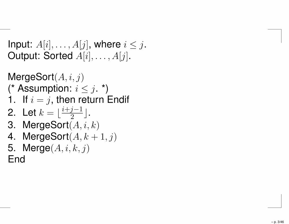
Input: A[i], . . . , A[j], where i ≤ j.Output: Sorted A[i], . . . , A[j].

MergeSort(A, i, j)(* Assumption: i ≤ j. *)1. If i = j, then return Endif

2. Let k = ⌊ i+j−12⌋.

3. MergeSort(A, i, k)4. MergeSort(A, k + 1, j)5. Merge(A, i, k, j)End

– p. 3/46

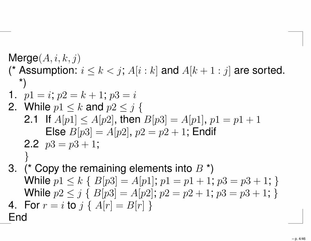
Merge(A, i, k, j)(* Assumption: i ≤ k < j; A[i : k] and A[k + 1 : j] are sorted.

*)1. p1 = i; p2 = k + 1; p3 = i2. While p1 ≤ k and p2 ≤ j

2.1 If A[p1] ≤ A[p2], then B[p3] = A[p1], p1 = p1 + 1Else B[p3] = A[p2], p2 = p2 + 1; Endif

2.2 p3 = p3 + 1;

3. (* Copy the remaining elements into B *)While p1 ≤ k B[p3] = A[p1]; p1 = p1 + 1; p3 = p3 + 1; While p2 ≤ j B[p3] = A[p2]; p2 = p2 + 1; p3 = p3 + 1;

4. For r = i to j A[r] = B[r] End

– p. 4/46

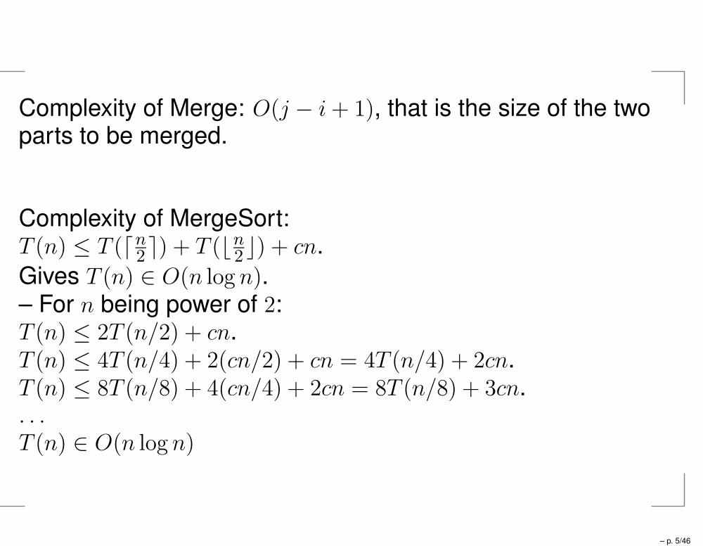
Complexity of Merge: O(j − i+ 1), that is the size of the twoparts to be merged.

Complexity of MergeSort:T (n) ≤ T (⌈n

2⌉) + T (⌊n

2⌋) + cn.

Gives T (n) ∈ O(n log n).– For n being power of 2:T (n) ≤ 2T (n/2) + cn.T (n) ≤ 4T (n/4) + 2(cn/2) + cn = 4T (n/4) + 2cn.T (n) ≤ 8T (n/8) + 4(cn/4) + 2cn = 8T (n/8) + 3cn.. . .T (n) ∈ O(n log n)

– p. 5/46

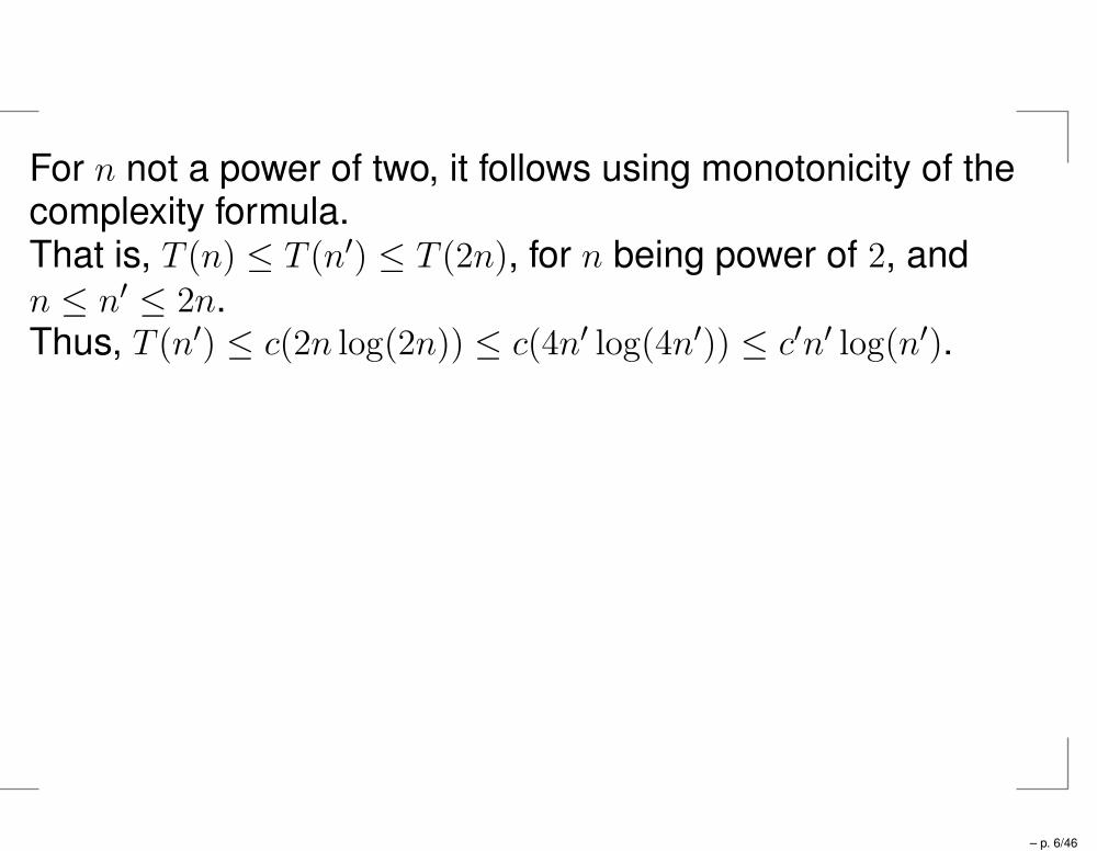
For n not a power of two, it follows using monotonicity of thecomplexity formula.That is, T (n) ≤ T (n′) ≤ T (2n), for n being power of 2, andn ≤ n′ ≤ 2n.Thus, T (n′) ≤ c(2n log(2n)) ≤ c(4n′ log(4n′)) ≤ c′n′ log(n′).

– p. 6/46

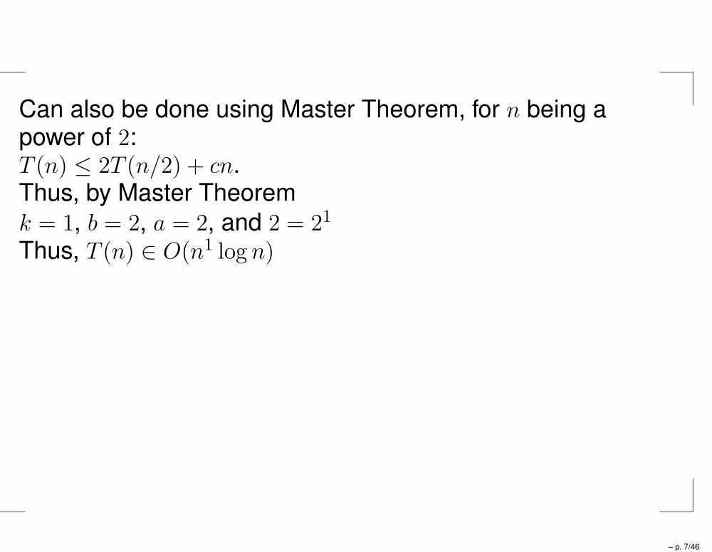
Can also be done using Master Theorem, for n being apower of 2:T (n) ≤ 2T (n/2) + cn.Thus, by Master Theorem

k = 1, b = 2, a = 2, and 2 = 21

Thus, T (n) ∈ O(n1 log n)

– p. 7/46

Average Case also Θ(n log n)

Stable.

Uses extra space for merging: O(n)

– p. 8/46

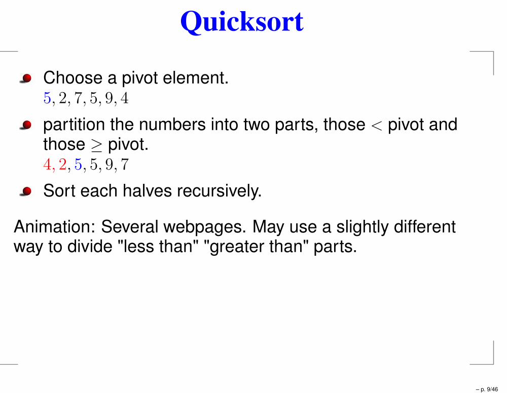
Quicksort

Choose a pivot element.5, 2, 7, 5, 9, 4

partition the numbers into two parts, those < pivot andthose ≥ pivot.4, 2, 5, 5, 9, 7

Sort each halves recursively.

Animation: Several webpages. May use a slightly differentway to divide "less than" "greater than" parts.

– p. 9/46

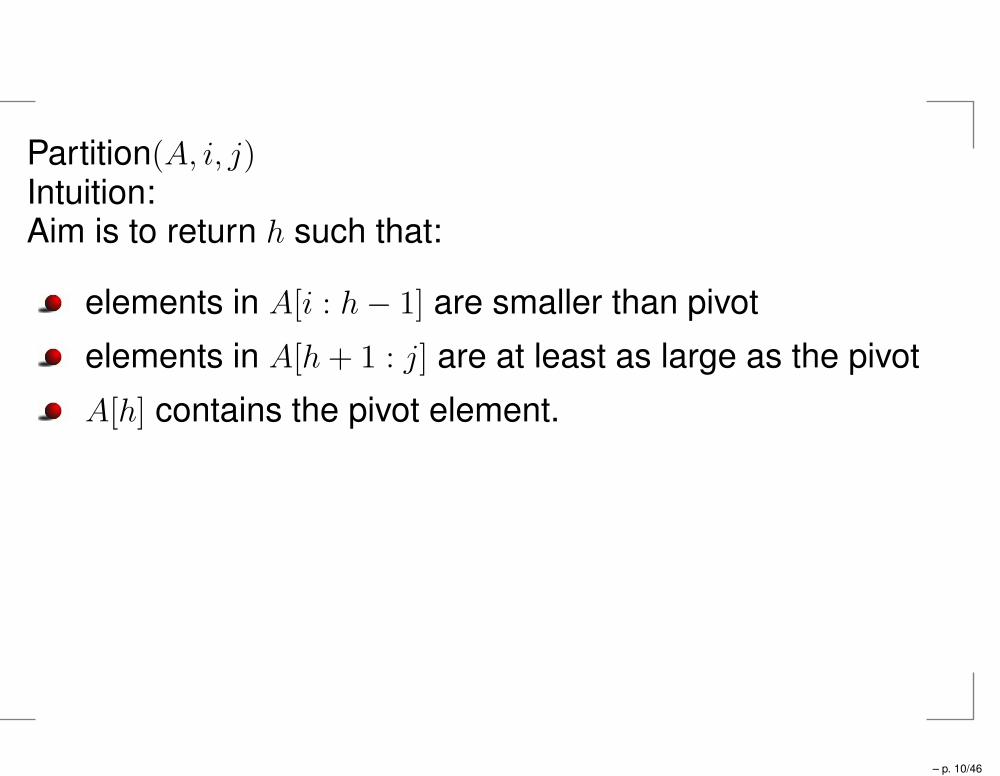
Partition(A, i, j)Intuition:Aim is to return h such that:

elements in A[i : h− 1] are smaller than pivot

elements in A[h+ 1 : j] are at least as large as the pivot

A[h] contains the pivot element.

– p. 10/46

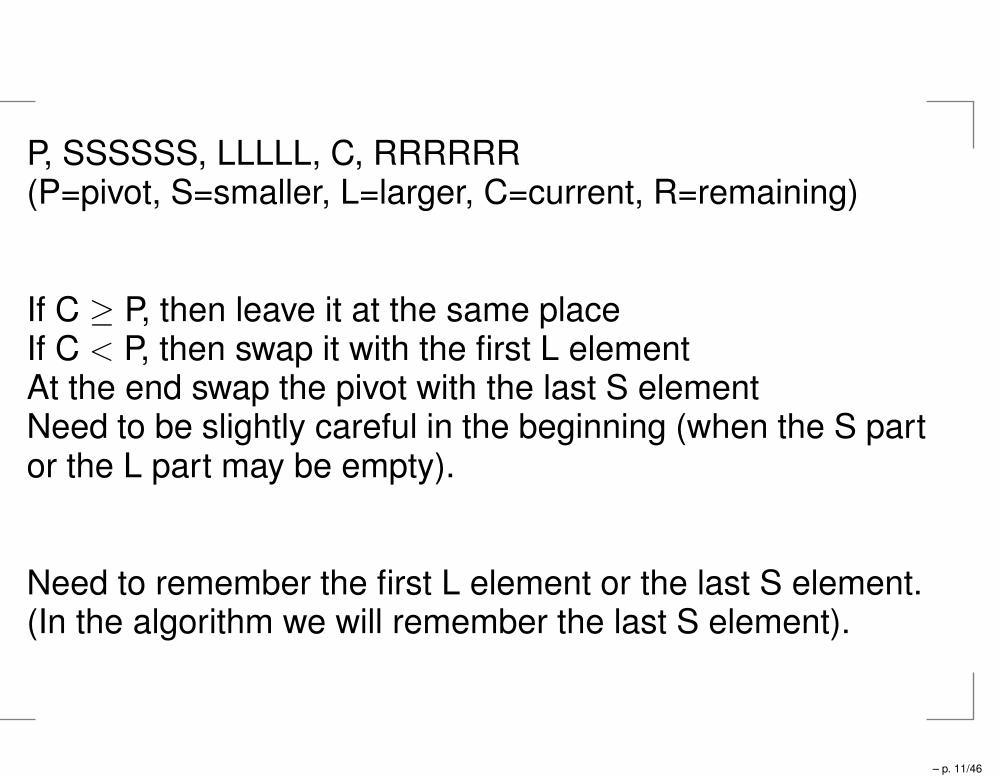
P, SSSSSS, LLLLL, C, RRRRRR(P=pivot, S=smaller, L=larger, C=current, R=remaining)

If C ≥ P, then leave it at the same placeIf C < P, then swap it with the first L elementAt the end swap the pivot with the last S elementNeed to be slightly careful in the beginning (when the S partor the L part may be empty).

Need to remember the first L element or the last S element.(In the algorithm we will remember the last S element).

– p. 11/46

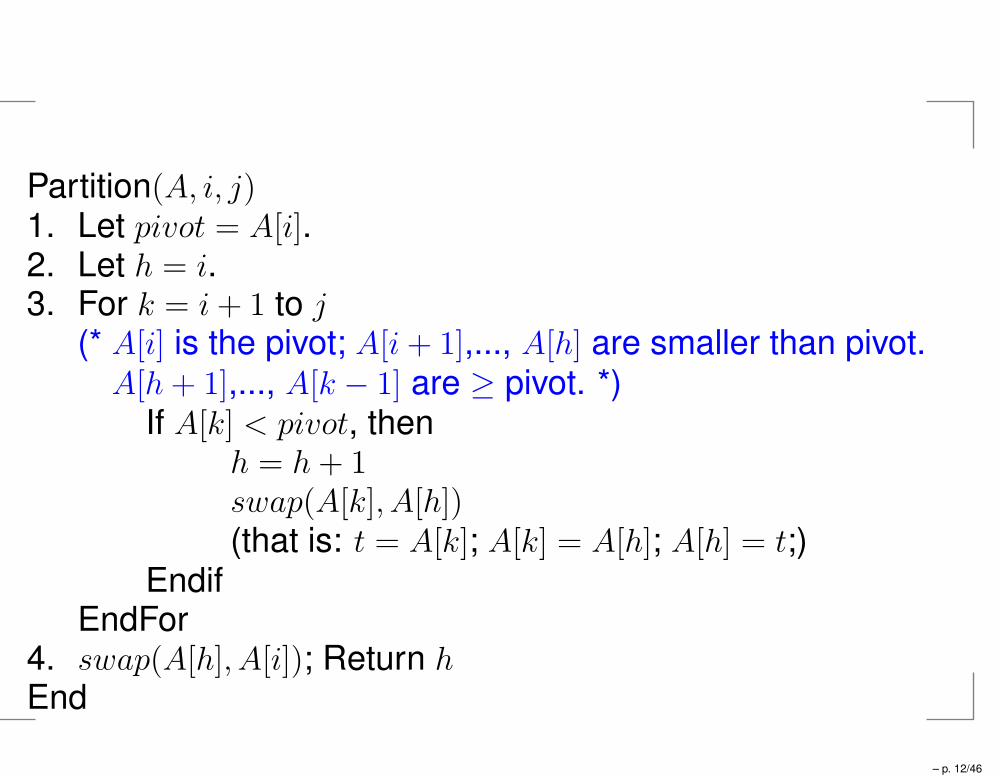
Partition(A, i, j)1. Let pivot = A[i].2. Let h = i.3. For k = i+ 1 to j

(* A[i] is the pivot; A[i+ 1],..., A[h] are smaller than pivot.A[h+ 1],..., A[k − 1] are ≥ pivot. *)

If A[k] < pivot, thenh = h+ 1swap(A[k], A[h])(that is: t = A[k]; A[k] = A[h]; A[h] = t;)

EndifEndFor

4. swap(A[h], A[i]); Return hEnd

– p. 12/46

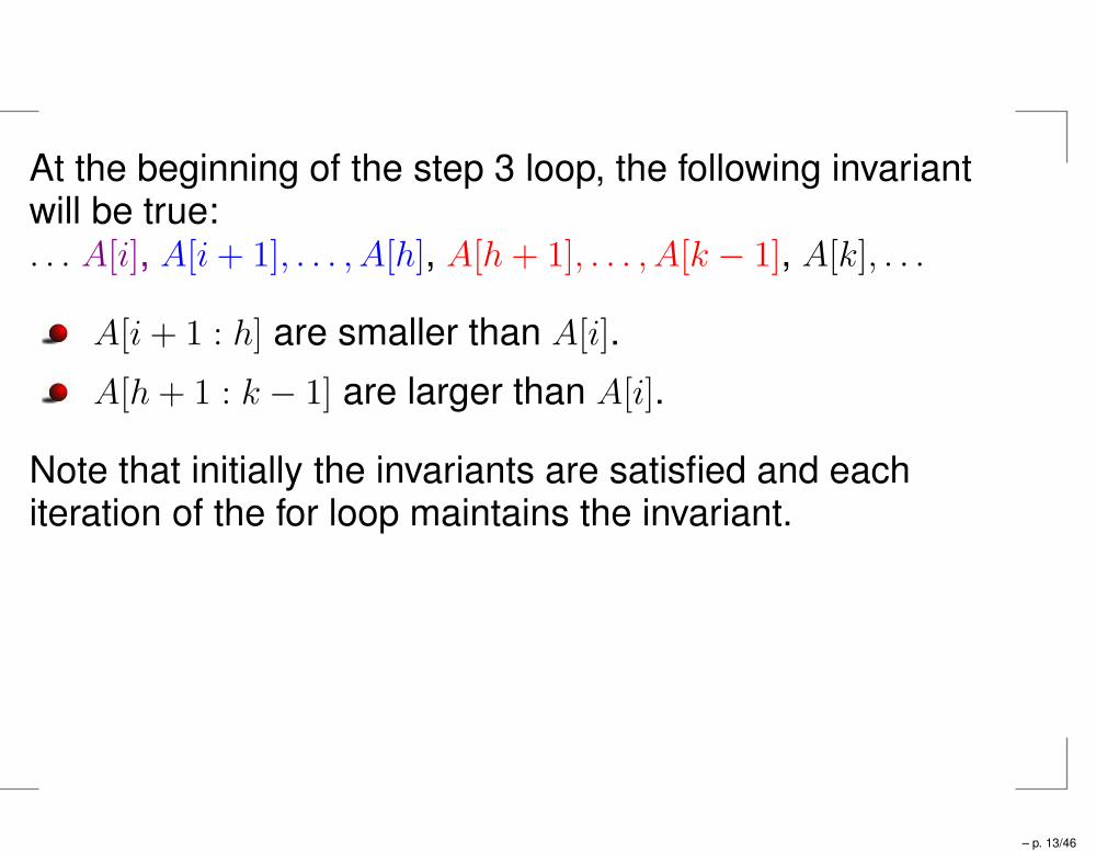
At the beginning of the step 3 loop, the following invariantwill be true:. . . A[i], A[i+ 1], . . . , A[h], A[h+ 1], . . . , A[k − 1], A[k], . . .

A[i+ 1 : h] are smaller than A[i].

A[h+ 1 : k − 1] are larger than A[i].

Note that initially the invariants are satisfied and eachiteration of the for loop maintains the invariant.

– p. 13/46

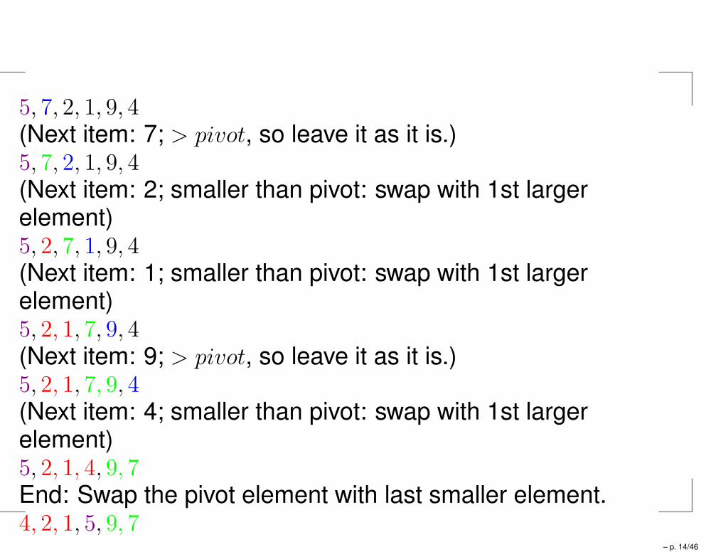
5, 7, 2, 1, 9, 4(Next item: 7; > pivot, so leave it as it is.)5, 7, 2, 1, 9, 4(Next item: 2; smaller than pivot: swap with 1st largerelement)5, 2, 7, 1, 9, 4(Next item: 1; smaller than pivot: swap with 1st largerelement)5, 2, 1, 7, 9, 4(Next item: 9; > pivot, so leave it as it is.)5, 2, 1, 7, 9, 4(Next item: 4; smaller than pivot: swap with 1st largerelement)5, 2, 1, 4, 9, 7End: Swap the pivot element with last smaller element.4, 2, 1, 5, 9, 7

– p. 14/46

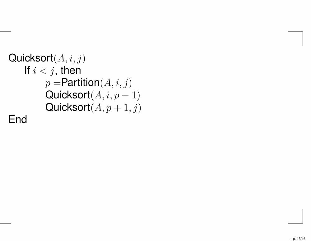
Quicksort(A, i, j)If i < j, then

p =Partition(A, i, j)Quicksort(A, i, p− 1)Quicksort(A, p+ 1, j)

End

– p. 15/46

Correctness:1. Partition does its job correctly.2. Assuming Partition does its job correctly, Quicksort doesits job correctly.

– p. 16/46

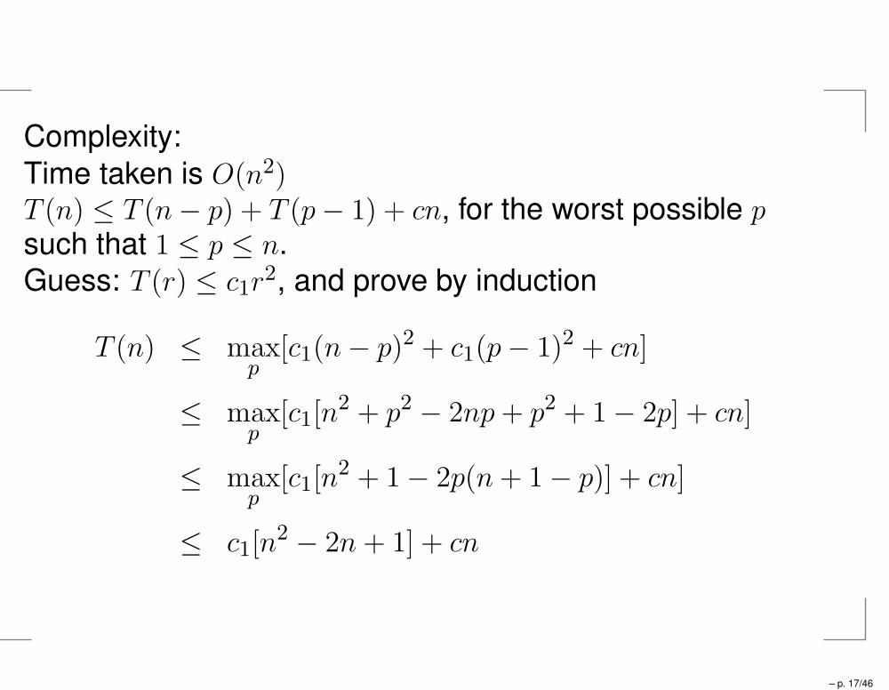
Complexity:

Time taken is O(n2)T (n) ≤ T (n− p) + T (p− 1) + cn, for the worst possible psuch that 1 ≤ p ≤ n.

Guess: T (r) ≤ c1r2, and prove by induction

T (n) ≤ maxp

[c1(n− p)2 + c1(p− 1)2 + cn]

≤ maxp

[c1[n2 + p2 − 2np+ p2 + 1− 2p] + cn]

≤ maxp

[c1[n2 + 1− 2p(n+ 1− p)] + cn]

≤ c1[n2 − 2n+ 1] + cn

– p. 17/46

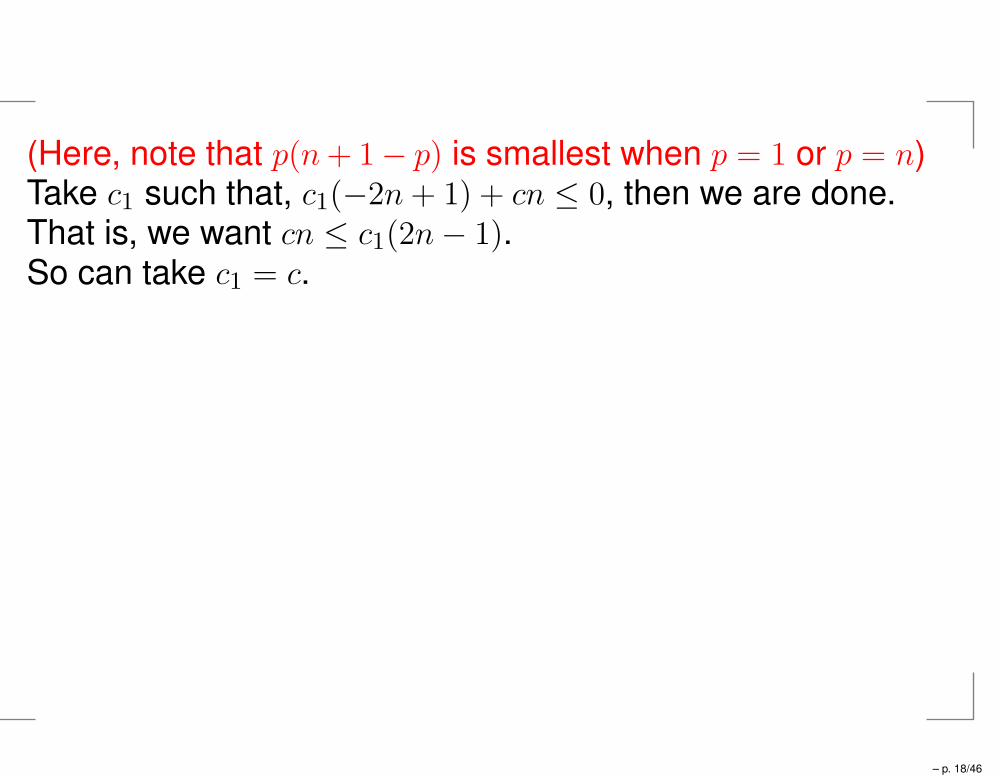
(Here, note that p(n+ 1− p) is smallest when p = 1 or p = n)Take c1 such that, c1(−2n+ 1) + cn ≤ 0, then we are done.That is, we want cn ≤ c1(2n− 1).So can take c1 = c.

– p. 18/46

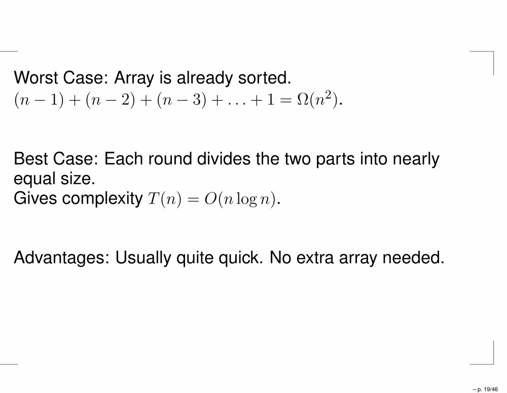
Worst Case: Array is already sorted.

(n− 1) + (n− 2) + (n− 3) + . . .+ 1 = Ω(n2).

Best Case: Each round divides the two parts into nearlyequal size.Gives complexity T (n) = O(n log n).

Advantages: Usually quite quick. No extra array needed.

– p. 19/46

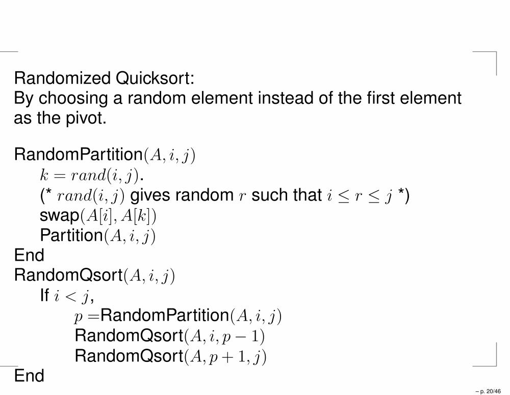
Randomized Quicksort:By choosing a random element instead of the first elementas the pivot.

RandomPartition(A, i, j)k = rand(i, j).(* rand(i, j) gives random r such that i ≤ r ≤ j *)swap(A[i], A[k])Partition(A, i, j)

EndRandomQsort(A, i, j)

If i < j,p =RandomPartition(A, i, j)RandomQsort(A, i, p− 1)RandomQsort(A, p+ 1, j)

End– p. 20/46

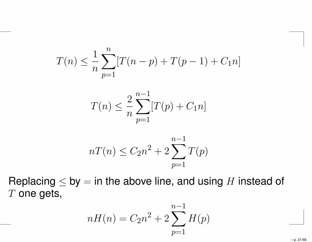
T (n) ≤1

n

n∑

p=1

[T (n− p) + T (p− 1) + C1n]

T (n) ≤2

n

n−1∑

p=1

[T (p) + C1n]

nT (n) ≤ C2n2 + 2

n−1∑

p=1

T (p)

Replacing ≤ by = in the above line, and using H instead ofT one gets,

nH(n) = C2n2 + 2

n−1∑

p=1

H(p)

– p. 21/46

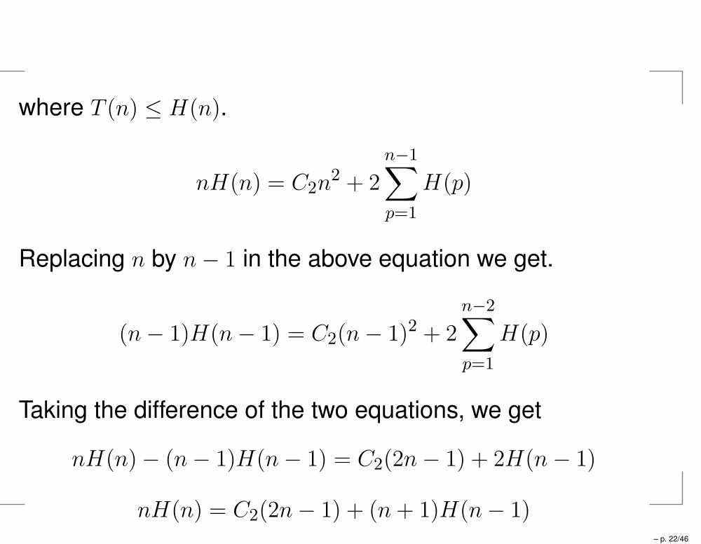
where T (n) ≤ H(n).

nH(n) = C2n2 + 2

n−1∑

p=1

H(p)

Replacing n by n− 1 in the above equation we get.

(n− 1)H(n− 1) = C2(n− 1)2 + 2

n−2∑

p=1

H(p)

Taking the difference of the two equations, we get

nH(n)− (n− 1)H(n− 1) = C2(2n− 1) + 2H(n− 1)

nH(n) = C2(2n− 1) + (n+ 1)H(n− 1)– p. 22/46

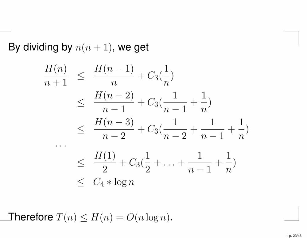
By dividing by n(n+ 1), we get

H(n)

n+ 1≤

H(n− 1)

n+ C3(

1

n)

≤H(n− 2)

n− 1+ C3(

1

n− 1+

1

n)

≤H(n− 3)

n− 2+ C3(

1

n− 2+

1

n− 1+

1

n)

. . .

≤H(1)

2+ C3(

1

2+ . . . +

1

n− 1+

1

n)

≤ C4 ∗ log n

Therefore T (n) ≤ H(n) = O(n logn).

– p. 23/46

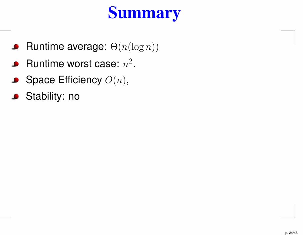
Summary

Runtime average: Θ(n(log n))

Runtime worst case: n2.

Space Efficiency O(n),

Stability: no

– p. 24/46

Binary Search

Input is Sorted.

Want to find whether a key K is present in the input.

Divide and conquer, but only ‘one half’ is relevant forcontinuation

Can thus easily be implemented iteratively.

– p. 25/46

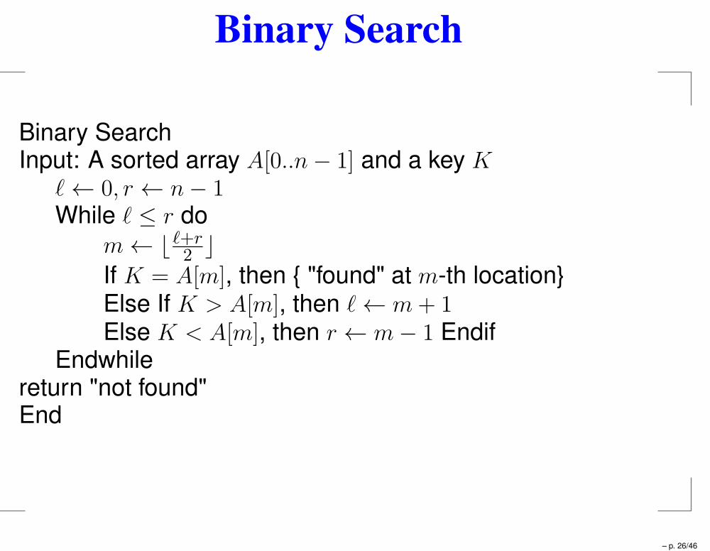
Binary Search

Binary SearchInput: A sorted array A[0..n− 1] and a key K

ℓ← 0, r ← n− 1While ℓ ≤ r do

m← ⌊ ℓ+r2⌋

If K = A[m], then "found" at m-th locationElse If K > A[m], then ℓ← m+ 1Else K < A[m], then r ← m− 1 Endif

Endwhilereturn "not found"End

– p. 26/46

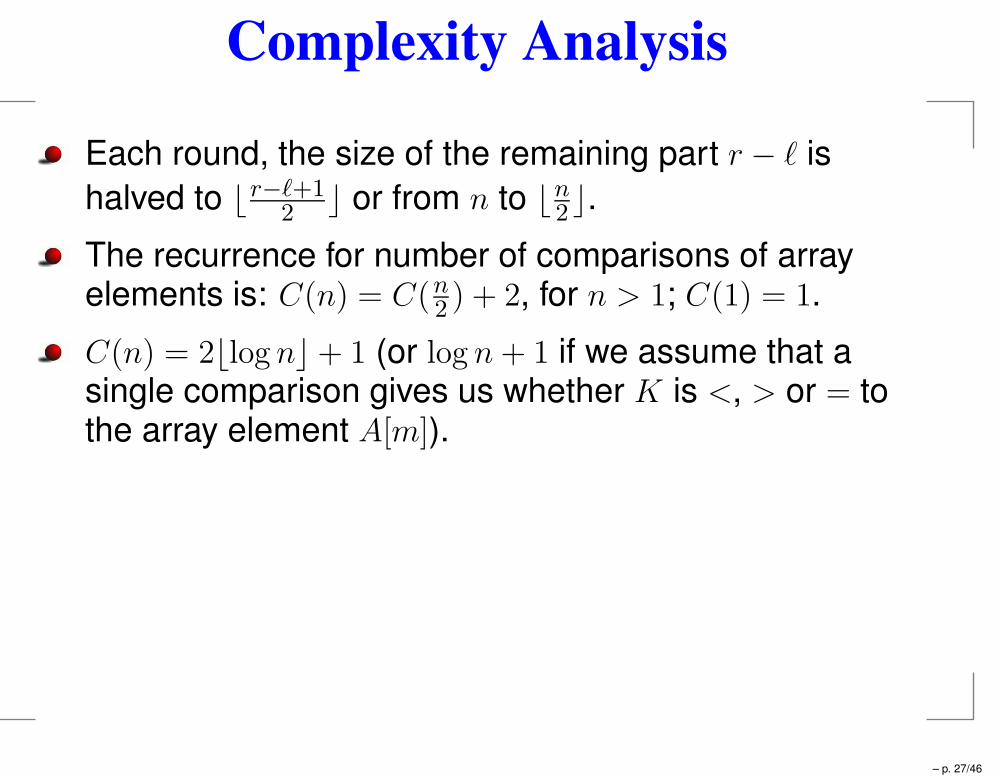
Complexity Analysis

Each round, the size of the remaining part r − ℓ is

halved to ⌊r−ℓ+12⌋ or from n to ⌊n

2⌋.

The recurrence for number of comparisons of arrayelements is: C(n) = C(n

2) + 2, for n > 1; C(1) = 1.

C(n) = 2⌊log n⌋+ 1 (or log n+ 1 if we assume that asingle comparison gives us whether K is <, > or = tothe array element A[m]).

– p. 27/46

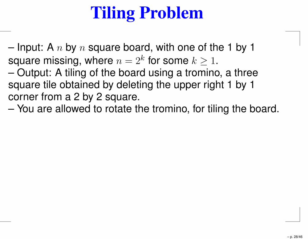
Tiling Problem

– Input: A n by n square board, with one of the 1 by 1

square missing, where n = 2k for some k ≥ 1.– Output: A tiling of the board using a tromino, a threesquare tile obtained by deleting the upper right 1 by 1corner from a 2 by 2 square.– You are allowed to rotate the tromino, for tiling the board.

– p. 28/46

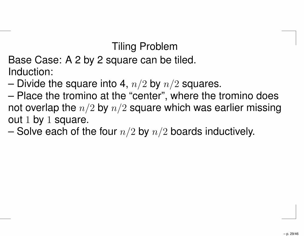
Tiling Problem

Base Case: A 2 by 2 square can be tiled.Induction:– Divide the square into 4, n/2 by n/2 squares.– Place the tromino at the “center”, where the tromino doesnot overlap the n/2 by n/2 square which was earlier missingout 1 by 1 square.– Solve each of the four n/2 by n/2 boards inductively.

– p. 29/46

Complexity: T (n) = 4T (n/2) + c.

Gives, T (n) = Θ(n2) using the master recurrence theorem.

Another way: There are (n2 − 1)/3 tiles to be placed, andplacing each tile takes O(1) time!

– p. 30/46

Traversals on a Binary Tree

Binary tree: Empty or (Root, left binary subtree, rightbinary subtree).

Full Binary tree: Either no or two children for each node.

Internal Node, leaf

For Full binary tree, number of leaves ℓ and number ofinternal nodes i is related as follows:2i = i+ ℓ− 1, as every internal node as two children,and total number of children is i+ ℓ− 1.Thus, i = ℓ− 1

– p. 31/46

Height of a binary tree/node

Height of single node is 0.

Height (T)Input: A tree T

If T = ∅, then return −1.Let TL and TR be the two children of the root of Treturn max(Height(TR), Height(TL)) + 1

End

– p. 32/46

Analysis

Consider attaching “null children” to each of the nodesof the tree T

The above algorithm visits every node, as well as thenull children mentioned above

n + n+ 1 nodes/null children visited

Total complexity is thus C(n) = 2n+ 1

Counting number of additions/Max: Once for eachnode. Total = n.

– p. 33/46

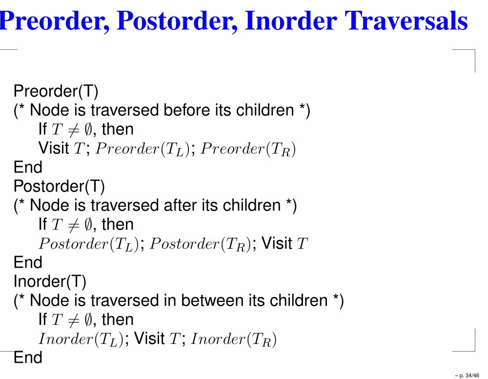
Preorder, Postorder, Inorder Traversals

Preorder(T)(* Node is traversed before its children *)

If T 6= ∅, thenVisit T ; Preorder(TL); Preorder(TR)

EndPostorder(T)(* Node is traversed after its children *)

If T 6= ∅, thenPostorder(TL); Postorder(TR); Visit T

EndInorder(T)(* Node is traversed in between its children *)

If T 6= ∅, thenInorder(TL); Visit T ; Inorder(TR)

End– p. 34/46

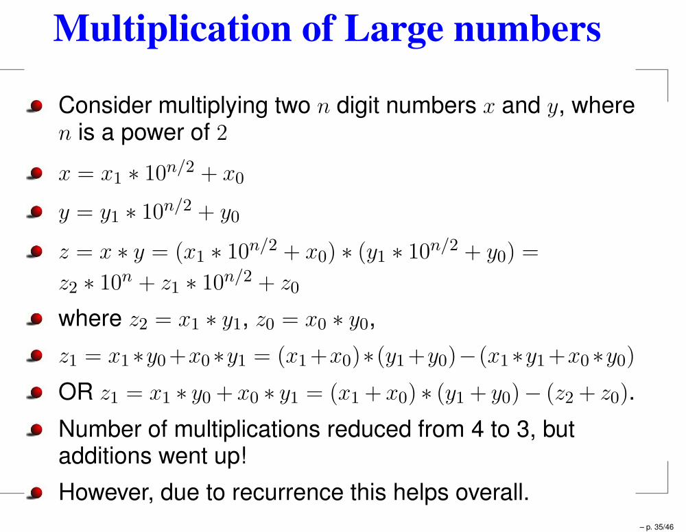
Multiplication of Large numbers

Consider multiplying two n digit numbers x and y, wheren is a power of 2

x = x1 ∗ 10n/2 + x0

y = y1 ∗ 10n/2 + y0

z = x ∗ y = (x1 ∗ 10n/2 + x0) ∗ (y1 ∗ 10

n/2 + y0) =

z2 ∗ 10n + z1 ∗ 10

n/2 + z0

where z2 = x1 ∗ y1, z0 = x0 ∗ y0,

z1 = x1∗y0+x0∗y1 = (x1+x0)∗(y1+y0)−(x1∗y1+x0∗y0)

OR z1 = x1 ∗ y0 + x0 ∗ y1 = (x1 + x0) ∗ (y1 + y0)− (z2 + z0).

Number of multiplications reduced from 4 to 3, butadditions went up!

However, due to recurrence this helps overall.

– p. 35/46

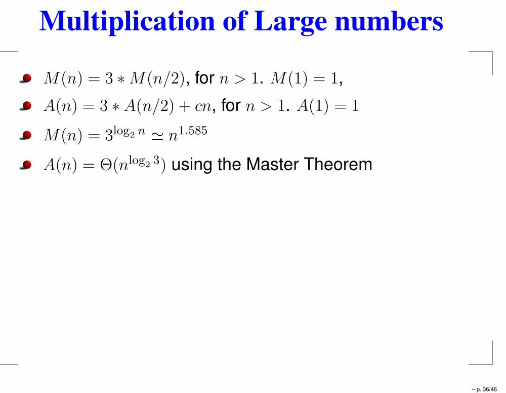
Multiplication of Large numbers

M(n) = 3 ∗M(n/2), for n > 1. M(1) = 1,

A(n) = 3 ∗ A(n/2) + cn, for n > 1. A(1) = 1

M(n) = 3log2 n ≃ n1.585

A(n) = Θ(nlog2 3) using the Master Theorem

– p. 36/46

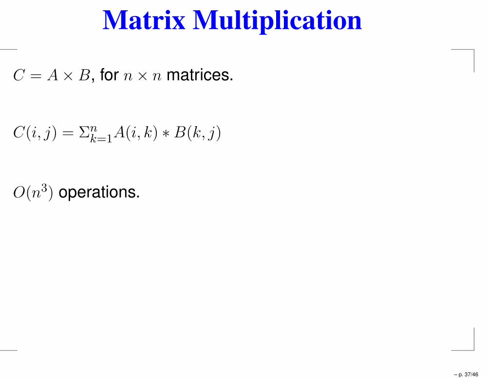
Matrix Multiplication

C = A× B, for n× n matrices.

C(i, j) = Σnk=1A(i, k) ∗ B(k, j)

O(n3) operations.

– p. 37/46

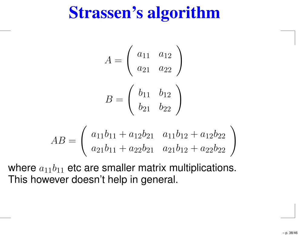
Strassen’s algorithm

A =

(

a11 a12

a21 a22

)

B =

(

b11 b12

b21 b22

)

AB =

(

a11b11 + a12b21 a11b12 + a12b22

a21b11 + a22b21 a21b12 + a22b22

)

where a11b11 etc are smaller matrix multiplications.This however doesn’t help in general.

– p. 38/46

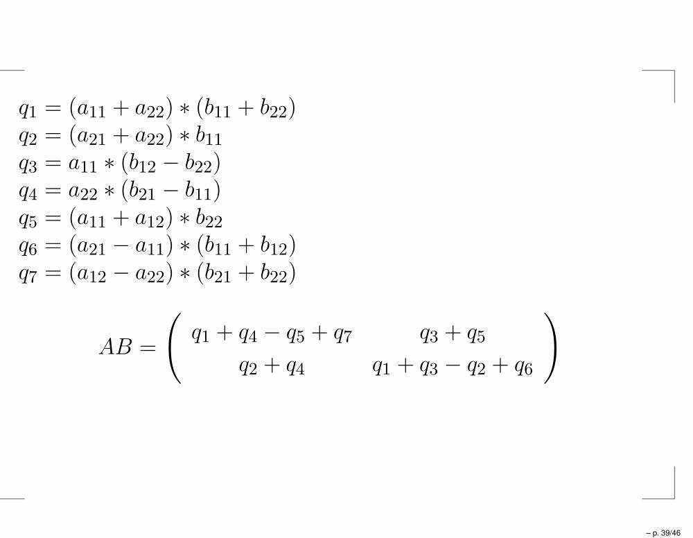
q1 = (a11 + a22) ∗ (b11 + b22)q2 = (a21 + a22) ∗ b11q3 = a11 ∗ (b12 − b22)q4 = a22 ∗ (b21 − b11)q5 = (a11 + a12) ∗ b22q6 = (a21 − a11) ∗ (b11 + b12)q7 = (a12 − a22) ∗ (b21 + b22)

AB =

(

q1 + q4 − q5 + q7 q3 + q5

q2 + q4 q1 + q3 − q2 + q6

)

– p. 39/46

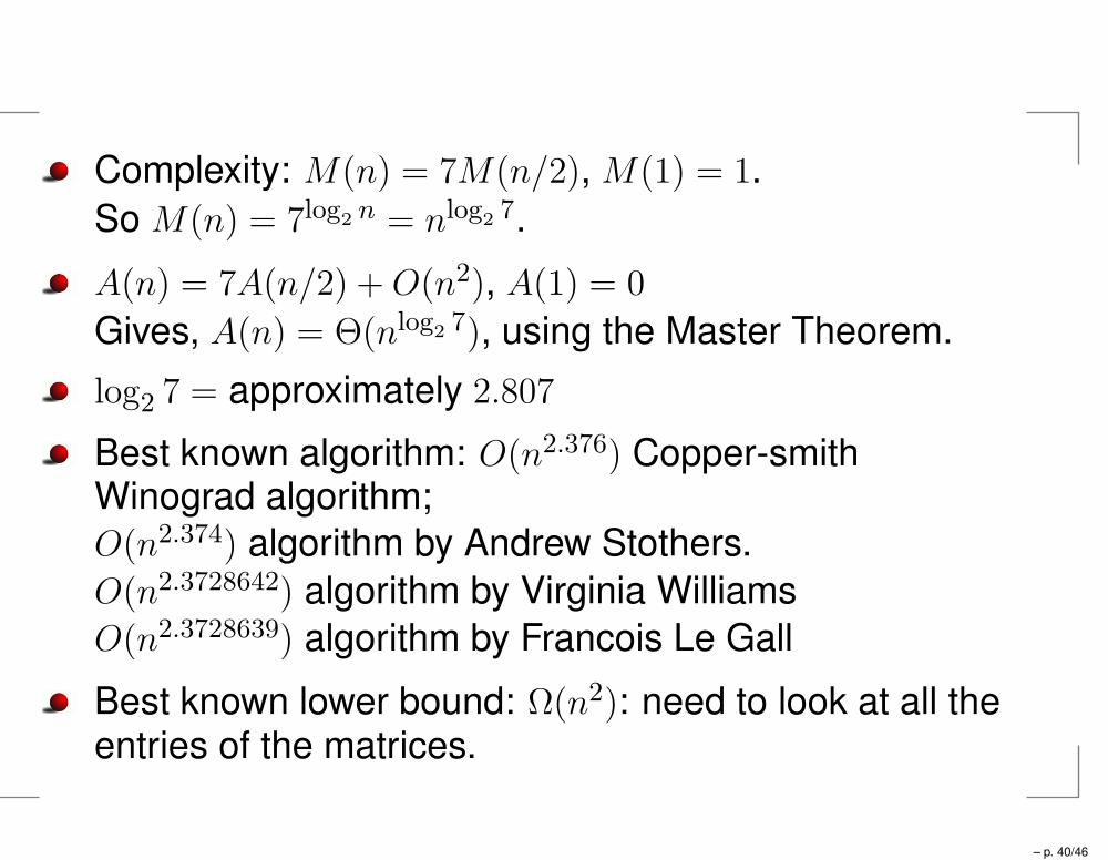
Complexity: M(n) = 7M(n/2), M(1) = 1.

So M(n) = 7log2 n = nlog2 7.

A(n) = 7A(n/2) +O(n2), A(1) = 0

Gives, A(n) = Θ(nlog2 7), using the Master Theorem.

log2 7 = approximately 2.807

Best known algorithm: O(n2.376) Copper-smithWinograd algorithm;

O(n2.374) algorithm by Andrew Stothers.

O(n2.3728642) algorithm by Virginia Williams

O(n2.3728639) algorithm by Francois Le Gall

Best known lower bound: Ω(n2): need to look at all theentries of the matrices.

– p. 40/46

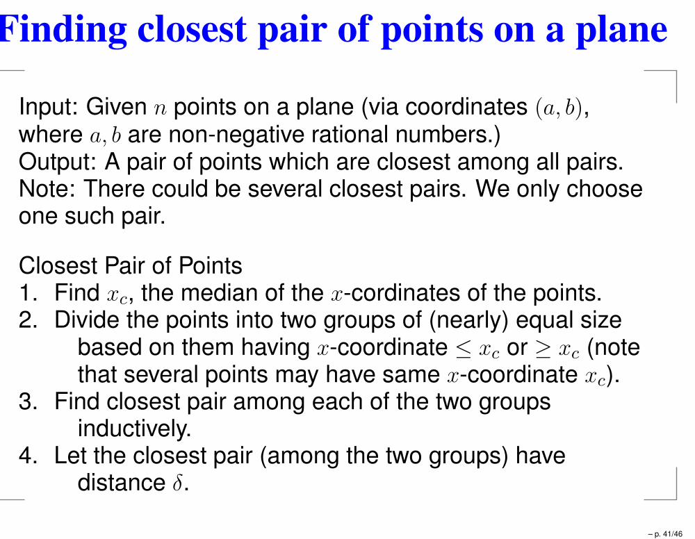
Finding closest pair of points on a plane

Input: Given n points on a plane (via coordinates (a, b),where a, b are non-negative rational numbers.)Output: A pair of points which are closest among all pairs.Note: There could be several closest pairs. We only chooseone such pair.

Closest Pair of Points1. Find xc, the median of the x-cordinates of the points.2. Divide the points into two groups of (nearly) equal size

based on them having x-coordinate ≤ xc or ≥ xc (notethat several points may have same x-coordinate xc).

3. Find closest pair among each of the two groupsinductively.

4. Let the closest pair (among the two groups) havedistance δ.

– p. 41/46

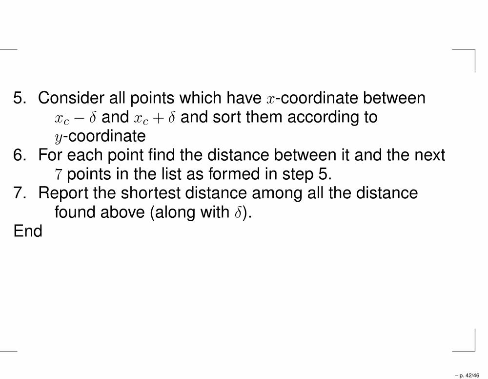
5. Consider all points which have x-coordinate betweenxc − δ and xc + δ and sort them according toy-coordinate

6. For each point find the distance between it and the next7 points in the list as formed in step 5.

7. Report the shortest distance among all the distancefound above (along with δ).

End

– p. 42/46

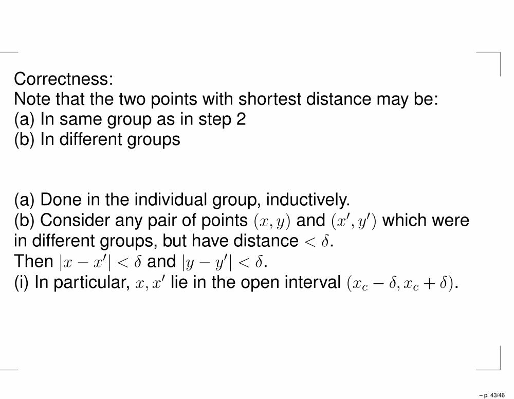
Correctness:Note that the two points with shortest distance may be:(a) In same group as in step 2(b) In different groups

(a) Done in the individual group, inductively.(b) Consider any pair of points (x, y) and (x′, y′) which werein different groups, but have distance < δ.Then |x− x′| < δ and |y − y′| < δ.(i) In particular, x, x′ lie in the open interval (xc − δ, xc + δ).

– p. 43/46

(xc − δ, (xc −δ2, (xc, (xc +

δ2, (xc + δ,

y + δ) y + δ) y + δ) y + δ) y + δ)

(xc − δ, (xc −δ2, (xc, (xc +

δ2, (xc + δ,

y + δ2) y + δ

2) y + δ

2) y + δ

2) y + δ

2)

(xc − δ, (xc −δ2, (xc, (xc +

δ2, (xc + δ,

y) y) y) y) y)

– p. 44/46

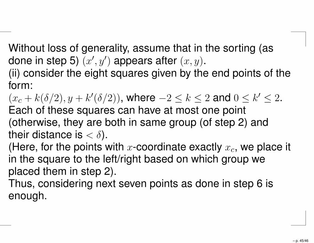
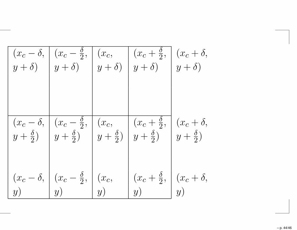
Without loss of generality, assume that in the sorting (asdone in step 5) (x′, y′) appears after (x, y).(ii) consider the eight squares given by the end points of theform:(xc + k(δ/2), y + k′(δ/2)), where −2 ≤ k ≤ 2 and 0 ≤ k′ ≤ 2.Each of these squares can have at most one point(otherwise, they are both in same group (of step 2) andtheir distance is < δ).(Here, for the points with x-coordinate exactly xc, we place itin the square to the left/right based on which group weplaced them in step 2).Thus, considering next seven points as done in step 6 isenough.

– p. 45/46

Complexity:T (n) ≤ 2T (⌈n

2⌉) + cn log n.

Gives T (n) = O(n(logn)2).

Smarter way: Don’t need to sort every time, but only once(before the start of the algorithm). This will giveT (n) ≤ 2T (⌈n

2⌉) + cn.

– p. 46/46