Global biogeography of atmosphericmicroorganisms re�ects diverse recruitment andenvironmental �lteringStephen Archer 

Auckland University of TechnologyKevin Lee 

Auckland University of TechnologyTancredi Caruso 

University College DublinMarcus Leung 

City University of Hong Kong https://orcid.org/0000-0002-6342-8181Xinzhao Tong 

City University of Hong KongSusannah J. Salter 

University of CambridgeGraham Hinchliffe 

Auckland University of TechnologyTeruya Maki 

Kindai UniversityTina Santl-Temkiv 

Aarhus UniversityKimberley Warren-Rhodes 

NASA Ames Research CenterBenito Gomez-Silva 

Universidad de AntofagastaKevin Hyde 

Mae Fah Luang UniversityCeline Liu 

Yale-NUS CollegeAntonio Alcamí 

Centro de Biología Molecular Severo Ochoa https://orcid.org/0000-0002-3333-6016Dina Al-Mailem 

Kuwait UniversityJonathan Araya 

Universidad de AntofagastaStephen Cary 

University of WaikatoDon Cowan 

University of PretoriaJessica Dempsey 

East Asian ObservatoryClaudia Etchebehere 

Biological Research Institute Clemente EstableBatdelger Gantsetseg 

Institute of Meteorology, Hydrology and EnvironmentSean Hartery 

University of CanterburyMike Harvey 

National Institution for Water and AtmosphereKazuichi Hayakawa 

Kanazawa UniversityIan Hogg 

Canadian High Arctic Research Station, Polar Knowledge Canada, Cambridge Bay, Nunavut, Canada;and School of Science, University of Waikato, Hamilton, New ZealandMutsoe Inoue 

Kanazawa UniversityMayada Kansour 

Kuwait UniversityTim Lawrence 

Auckland University of TechnologyCharles Lee 

University of Waikato https://orcid.org/0000-0002-6562-4733Matthius Leopold 

University of Western AustraliaChristopher McKay 

NASA Ames Research centerSeiya Nagao 

Kanazawa UniversityYan Hong Poh 

Yale-NUS CollegeJean-Baptiste Ramond 

Ponti�cia Universidad Católica de Chile https://orcid.org/0000-0003-4790-6232Alberto Rastrojo 

Universidad Autonoma de MadridToshio Sekiguchi 

Kanazawa UniversityJoo Huang Sim 

Yale-NUS CollegeWilliam Stahm 

East Asian ObservatoryHenry Sun 

Desert Research InstituteNing Tang 

Kanazawa University https://orcid.org/0000-0002-3106-6534Bryan Vandenbrink 

Canadian High Arctic Research StationCraig Walther 

East Asian ObservatoryPatrick Lee 

City Universiy of Hong Kong https://orcid.org/0000-0003-0911-5317Stephen Brian Pointing  ( stephen.pointing@yale-nus.edu.sg )

National University of Singapore https://orcid.org/0000-0002-7547-7714

Research Article

Keywords: atmospheric microbiology, microbial ecology, global ecosystem

Posted Date: February 9th, 2022

DOI: https://doi.org/10.21203/rs.3.rs-244923/v4

License: This work is licensed under a Creative Commons Attribution 4.0 International License.  Read Full License

1

Global biogeography of atmospheric microorganisms reflects diverse recruitment and 1

environmental filtering 2

3

Stephen D.J. Archer1, Kevin C. Lee1, Tancredi Caruso2, Marcus H.Y. Leung3, Xinzhao 4

Tong3, Susannah J Salter4, Graham Hinchliffe1, Teruya Maki5, Tina Santl-Temkiv6, 5

Kimberley A. Warren-Rhodes7,8, Benito Gomez-Silva9, Kevin D. Hyde10, Celine J.N. Liu11, 6

Antonio Alcami12, Dina M. Al Mailem13, Jonathan G.Araya14, S. Craig Cary15, Don A. 7

Cowan16, Jessica Dempsey17, Claudia Etchebehere18, Batdelger Gantsetseg19, Sean Hartery20, 8

Mike Harvey21, Kazuichi Hayakawa22, Ian Hogg23, Mutsoe Inoue22, Mayada K. Kansour13, 9

Timothy Lawrence1, Charles K. Lee15, Matthias Leopold24, Christopher P. McKay7, Seiya 10

Nagao22, Yan Hong Poh11, Jean-Baptiste Ramond25, Alberto Rastrojo12, Toshio Sekiguchi22, 11

Joo Huang Sim11, William Stahm17, Henry J. Sun26, Ning Tang22, Bryan Vandenbrink23, 12

Craig Walther17, Patrick K.H. Lee3, Stephen B. Pointing11,22,27* 13

14

1 School of Science, Auckland University of Technology, Auckland, New Zealand 15

2 School of Biology and Environmental Science, University College Dublin, Dublin, Ireland 16

3 School of Energy and Environment, City University of Hong Kong, Hong Kong, China 17

4 Department of Veterinary Medicine, University of Cambridge, Cambridge, United Kingdom 18

5 Department of Life Sciences, Kindai University, Osaka, Japan 19

6 Department of Biology, Aarhus University, Aarhus, Denmark 20

7 NASA Ames Research Center, Mountain View, California, USA 21

8 SETI Institute, Mountain View, California, USA 22

9 Departamento Biomédico, Universidad de Antofagasta, Antofagasta, Chile 23

10 Center of Excellence in Fungal Diversity, Mae Fah Luang University, Chiang Rai, 24

Thailand 25

2

11 Yale-NUS College, National University of Singapore, Singapore 26

12 Centro de Biología Molecular Severo Ochoa, Consejo Superior de Investigaciones 27

Científicas (CSIC), Universidad Autónoma de Madrid, Madrid, Spain 28

13 Department of Biological Sciences, Kuwait University, Kuwait City, Kuwait 29

14 Instituto Antofagasta, Universidad de Antofagasta, Antofagasta, Chile 30

15 School of Science, University of Waikato, Hamilton, New Zealand 31

16 Department of Biochemistry, Genetics and Microbiology, University of Pretoria, Pretoria, 32

South Africa 33

17 East Asian Observatory, Hilo, Hawaii, USA 34

18 Biological Research Institute Clemente Estable, Ministry of Education, Montevideo, 35

Uruguay 36

19 Institute of Meteorology, Hydrology and Environment, Ulan Bator, Tuv, Mongolia 37

20 School of Physical and Chemical Sciences, University of Canterbury, Christchurch, New 38

Zealand 39

21 National Institute of Water and Atmospheric Research, Wellington, New Zealand 40

22 Institute of Nature and Environmental Technology, Kanazawa University, Kanazawa, 41

Japan 42

23 Canadian High Arctic Research Station, Cambridge Bay, Nunavut, Canada 43

24 UWA School of Agriculture and Environment, University of Western Australia, Perth, 44

Australia 45

25 Departamento de Genética Molecular y Microbiología, Pontificia Universidad Católica de 46

Chile, Santiago, Chile 47

26 Desert Research Institute, Las Vegas, Nevada, USA 48

27 Department of Biological Sciences, National University of Singapore, Singapore 49

*Corresponding author, e-mail yncpsb@nus.edu.sg 50

3

51

Competing Interests 52

The authors declare no competing interests. 53

54

Abstract 55

Atmospheric transport is critical to dispersal of microorganisms between habitats, and this 56

underpins resilience in terrestrial and marine ecosystems globally. A key unresolved question 57

is whether microorganisms assemble to form a taxonomically distinct, geographically 58

variable, and functionally adapted atmospheric microbiota. This question is made more 59

complex by the unique challenges of separating potential contaminants from atmospheric 60

signal, particularly given the ultra-low biomass of air and the long durations of sampling 61

where contamination may occur. Here we adopted a comprehensive data filtering approach to 62

mitigate contamination and characterise inter-continental patterns of microbial taxonomic and 63

functional diversity in air within and above the atmospheric boundary layer and in underlying 64

soils for 596 globally sourced samples. Bacterial and fungal assemblages in air were 65

taxonomically structured and deviated significantly from purely stochastic assembly. Patterns 66

differed with location and reflected climate, underlying surface cover and environmental 67

filtering. Source-tracking indicated a complex recruitment process involving local soils plus 68

globally distributed inputs from drylands and the phyllosphere. Assemblages displayed stress-69

response and metabolic traits relevant to survival in air, and taxonomic and functional 70

diversity were correlated with macroclimate and atmospheric variables. Our findings 71

highlight complexity in the atmospheric microbiota that is key to understanding regional and 72

global ecosystem connectivity. 73

74

Introduction 75

4

Microorganisms occupy central roles in terrestrial and marine ecosystems globally [1, 2]. 76

Movement of viable cells and propagules between habitats occurs largely through the 77

troposphere, which is the atmospheric layer closest to Earth [3, 4]. This is critical to 78

recruitment and turnover that drive ecological resilience of these systems [2–5], as well as 79

influencing dispersal of pathogens and invasive taxa [4, 6]. There is also a growing awareness 80

that microorganisms suspended in the atmosphere are potentially capable of in situ metabolic 81

and biophysical activities that can influence climatic processes [4, 7]. However, despite the 82

central importance of the atmosphere to these ecological outcomes, assessments of microbial 83

diversity in air at broad geographic scales remain limited [8, 9]. As a result, there is little 84

understanding of how variable the overall microbial composition of the atmosphere may be 85

on a global scale, the extent to which it may be decoupled from underlying local surface 86

communities that are the sources and sinks for atmospheric microorganisms, or the 87

importance of environmental or biotic factors in shaping diversity. The unique role of the 88

atmosphere as a transport medium for microorganisms has also obscured the question of 89

whether it supports a functionally adapted microbiome with the potential for metabolic 90

transformations and cell proliferation [3]. 91

Previous research has been hampered by lack of consensus for community structures 92

of atmospheric microbiota due to the different experimental approaches, lack of ecologically 93

relevant scaling and taxonomic resolution, and the confounding effect of contamination in the 94

ultra-low biomass atmospheric habitat [10–12]. Nonetheless, inferred community structure 95

for air at various locales within the near-ground atmospheric boundary layer where the bulk 96

of surface-atmosphere interactions occur have described bacterial and fungal communities 97

that were correlated with local abiotic variables such as temperature and humidity [13] or land 98

use [9, 14]. Several studies have related variation in communities to different history of 99

sampled air masses and this suggests combined influence of the different sources and 100

5

conditions to which microorganisms are exposed during transit [15–18]. Indirect surveys from 101

ground-deposited desert dust [19] or precipitation [20] have yielded valuable insight on long-102

range dispersal across inter-continental scales although they reflect deposition and differ 103

somewhat to direct estimates from air [17]. Sampling in the free troposphere at higher 104

altitudes above the atmospheric boundary layer is challenging and scarce data indicates a 105

more restricted microbial occurrence [21]. Thus, the conventional dogma that atmospheric 106

transport is a neutral process involving ubiquitous distribution of taxa has been challenged by 107

recent theoretical [22, 23] and experimental advances [20, 24, 25]. Adaptive traits have 108

generally been inferred from taxonomy, although laboratory estimates of metabolic activity 109

by atmospheric bacterial isolates [26], and recovery of RNA from air and cloud water [27, 110

28], indicate that atmospheric microorganisms are potentially active in situ. Significant 111

research gaps persist and particularly with regard to discerning biogeographic patterns. This 112

requires standardised sampling across broad ecological scales and with comparative data from 113

surface habitats, and careful attention to decontamination of ultra-low biomass air samples. 114

Here we report findings testing our hypothesis that atmospheric microbial diversity is 115

distinct from that in underlying surface habitats, is non-randomly assembled, and 116

environmental filtering and diverse recruitment explain observed patterns. We characterised 117

taxonomic and functional diversity in a large globally sourced original dataset (n = 596) for 118

air within the atmospheric boundary layer that delineates the majority of physical interactions 119

with the Earth’s surface [29] (near-ground air), as well as aircraft sampling of free 120

tropospheric air at higher altitudes above the atmospheric boundary layer (high-altitude air). 121

We combined this with concurrent sampling of underlying surface soils and sediments to 122

allow direct air-surface connectivity comparisons. Importantly we conducted and report 123

extensive decontamination of sequence data in order to provide a confident diversity estimate 124

where the unavoidable sampling and reagent contamination due to the ultra-low biomass 125

6

atmospheric system must be carefully mitigated [10, 11]. We provide multiple lines of 126

evidence for a taxonomically distinct, non-randomly assembled, altitudinally, geographically 127

and functionally variable atmospheric microbiota that is influenced by a complex suite of 128

biotic and abiotic drivers. 129

130

Methods 131

Environmental and climate metadata and modelling 132

Local climate metadata for each sampling location were retrieved from public databases 133

(Supplementary notes on environmental metadata). Back trajectories and environmental 134

conditions that airborne microorganisms were exposed to during their transit towards each 135

sampling location was modelled from National Oceanic and Atmospheric Administration 136

(NOAA) atmospheric transport and dispersion models (Figs S1, S2) [30]. 137

Sample recovery 138

The sampling campaign retrieved 596 air and soil samples using stringent clean sampling 139

approaches from 18 locations spanning all major climatic regions and continents plus two 140

oceans (Table S1). Bulk phase air was recovered using Coriolis µ high-volume impingement 141

devices (Bertin Instruments) from the atmospheric boundary layer at 1.5m above the surface 142

(near-ground air, n = 501) and from the free troposphere at 2,000 m above local surface level 143

using aircraft mounted air samplers (high-altitude air, n = 11) (Supplementary information: 144

Supplementary notes on sample recovery, Fig. S3) [29]. Underlying soil was sampled 145

immediately after each air sampling was conducted (soil, n = 84). Ship-board sampling was 146

achieved at 25m above the ocean surface to avoid sea-spray contamination. Environmental 147

DNA was recovered from all samples and controls as previously described [25] and included 148

sampling and reagent controls for every location and processing batch (Supplementary 149

information: Supplementary notes on sample recovery). 150

7

Gene copy number estimation 151

Real-time quantitative PCR (qPCR) was employed for the most abundant microbial groups 152

(bacteria and fungi) [31]. Primers targeted the16S rRNA gene for bacteria [32, 33], and 18S 153

rRNA gene for fungi [34]. Reactions were performed as previously described [35]. A qPCR 154

standard for each target sequence was developed to estimate gene copy number using pooled 155

samples and serial dilutions of the template were used to generate standard curves. 156

Amplicon sequencing 157

Sequence libraries were prepared using Illumina MiSeq v3 600 cycle chemistry as per 158

manufacturer’s protocol. Template DNA in samples was normalised to 2.5ng/ul prior to two-159

step PCR amplification for the bacterial 16S rRNA gene V3-V4 hypervariable region ([32, 160

33], and fungal ITS1 region [36, 37] as previously described [25]. Libraries were first 161

processed with cutadapt v2.7 [38] to remove primer sequences and amplicon sequence 162

variants (ASVs [39]) were generated using dada2 v1.14 [40]. Pseudo-pooling was used in 163

ASV calling to increase sensitivity and detect rare ASVs. Taxonomic classification was 164

conducted in dada2 with SILVA v138 [41] and UNITE v7.2 [42] as references. Overall, the 165

amplicon sequencing generated 19.5 million bacterial reads and 1.7 million fungal reads and 166

these resolved to over 200,000 genuine ASVs. Diversity analysis occurred only after an 167

extensive best-practice decontamination protocol to mitigate putative contamination in 168

sequence libraries that is unavoidable when interrogating ultra-low biomass samples 169

(Supplementary Information: Decontamination of environmental sequence data, Figs S6-S21, 170

table S3) [10, 11, 43]. Briefly, this comprised subtractive filtering steps for ASVs as follows: 171

1) removal of non-target sequences; 2) Removal of ASVs with suspicious frequency (using 172

the default value of 0.1) and/or prevalence (using a more stringent threshold of 0.5) using 173

decontam [44]; 3) Removal of ASVs encountered in any of the sampling or reagent controls 174

from all samples; 4) A subtractive filtering at genus level of human-associated contaminants 175

8

regardless of whether or not they were also encountered in controls. Decontamination 176

outcomes were reported and post-hoc testing for residual contaminants conducted. All 177

sequence data were also screened for potential batch effects, cross-contamination, and spatial 178

and temporal autocorrelation. After the decontamination steps, true samples with > 1,000 179

reads (16S rRNA n = 529, ITS n = 444) were used for all subsequent analyses. Sampling 180

curves for all post-filtered air and soil samples achieved near-asymptote for ASV diversity. 181

Detailed description and data reporting for all steps is given in Supplementary information. 182

Shotgun metagenomics 183

Libraries were prepared using a low-input preparation protocol where required [45] and using 184

the Nextera XT library kit and sequenced (2 × 150 bp paired-end) on an Illumina NextSeq 185

500 (Illumina, USA). Kneaddata (v0.7.4, default settings, 186

https://github.com/biobakery/kneaddata) was used to remove low-quality reads and human 187

DNA using the human genome hG37 as reference from raw fastq files, and filtered reads 188

were further processed to identify and remove potential contaminating nearest taxonomic 189

units (NTUs) in a similar manner to that applied to ASVs (Supplementary information: 190

Decontamination of environmental sequence data). After all the decontamination steps, a total 191

of 1.5 billion high-quality paired-end reads were retained across the entire dataset of 120 192

metagenomes, averaging 12.5 million reads per sample. Taxonomic profiles (phylum and 193

species) of the high-quality reads were generated with Kraken2 [46], and Bracken [47], and 194

FindFungi [47]. Functional potentials of the metagenomes were queried using HUMAnN 195

(v3.0.0.alpha.3) [48], generating a total of 1.86 million unique features, which were 196

subsequently converted to over 10,000 protein families (Pfams) corresponding to genes 197

encoding carbon fixation, cold shock response, nitrogen cycle, oxidative stress, phototrophy, 198

respiration, sporulation, starvation, trace gas metabolism, and UV repair proteins (Table S2). 199

Statistical treatments and ecological modelling 200

9

Statistical analysis: General processing of the community data including the calculation of 201

relative abundance and estimates of alpha diversity were conducted using the R package 202

phyloseq [49] and visualised using ggplot2 [50]. Comparative statistical analyses were 203

performed using R: ANOVA, Kruskal-Wallis, Mann-Whitney test, Mantel test, 204

PERMANOVA, manyglm with negative binomial distribution using mvabund [51] (an 205

approach that takes into account heterogeneity in mean-variance relationships [52]), 206

Procrustes analysis using vegan [53], lmPerm (permutation test for ANOVA) (https://cran.r-207

project.org/web/packages/lmPerm/index.html), dunn.test (Dunn’s test for post hoc analysis, 208

P-values were adjusted by the Holm–Bonferroni method) (https://cran.r-209

project.org/web/packages/dunn.test/index.html), ANCOMBC (ancombc differential 210

abundance analysis, P-values were adjusted by the Holm–Bonferroni method) [54]. 211

Correlations used in compositional analysis of taxonomic data to determine potential residual 212

contaminants were calculated using FastSpar [55]. Calculation of geographic distances were 213

performed using R package geosphere [56] function distGeo with WGS84 ellipsoid. Source 214

tracking was conducted by fast expectation-maximization using FEAST [57] with data from 215

other studies (processed using dada2 following the same parameters as this study) as 216

additional sources/sinks [58–64] and NCBI BioProject PRJEB42801. For correlation analysis 217

between abiotic and biotic variables the Pearson correlation coefficient for multiple pairwise 218

combinations were calculated using the R package corrplot [65], with P-value cut-off of 0.05 219

corrected for multiple tests using Bonferroni correction. To visualise patterns of community 220

dissimilarity, two methods were used. Hellinger distances were ordinated with t-distributed 221

stochastic neighbour embedding (tSNE) using R package Rtsne [66]. Jaccard sample pair-222

wise distances were calculated using the R package vegan [53], and tested for locations and 223

habitat (i.e. soil, near ground air and high elevation air) using PERMANOVA [67]. The 224

Jaccard matrix was decomposed with Principal Coordinate Analysis (PCoA) to provide a 225

10

quantification of the variance accounted by each ordination axis [68]. Network null models 226

were employed to detect non-random structure (nestedness) in the microbial assemblages 227

(Supplementary information: Supplementary notes on the use of Null models, Figs S4, S5). A 228

statistical mechanics approach was employed for network construction [69], with networks 229

defined as bipartite matrices with two layers: location and taxa. Z‐scores for nestedness were 230

calculated using the commonly employed NODF metric to indicate the number of standard 231

deviations a given data point lay from the mean [70], and also using Jaccard distance to 232

estimate pair-wise assemblage dissimilarity and test if the average dissimilarity deviated from 233

that expected under random assembly. 234

235

Results 236

An overview of inter-domain diversity from our metagenomic libraries indicated that 237

composition was more variable in air than soil (average Bray-Curtis dissimilarity within air 238

samples = 0.256 vs. within soil samples = 0.038, Mann Whitney U = 8.7 × 107, P = < 2.2 × 239

10-16, Wendt effect size r = 0.493) (Fig. 1). Bacteria were the most abundant component of 240

soil and air metagenomes and fungi were the second highest microbial category in near-241

ground air. Relatively low and patchy contribution was observed for archaea and microbial 242

eukaryotes. We therefore focused further community profiling effort on bacteria and fungi 243

with shotgun metagenomics and targeted amplicon sequencing. Sampling of air microbiota 244

presents unique challenges in terms of potential contamination due to the ultra-low biomass 245

habitat. Extended sampling durations increase the potential for unintentional human 246

atmospheric transmission not well addressed with traditional negative controls used for other 247

ultra-low biomass samples, and rarely considered in atmospheric microbiology. Sequencing 248

of our 596 globally-sourced air and soil samples was therefore combined with an extensive 249

effort to mitigate against the occurrence of putative contaminant taxa and cross-contamination 250

11

that have plagued low-biomass microbiological studies using traditional negative controls, but 251

also necessitated the use of human controls and bioinformatic filtering of any potential 252

contamination taxa [10, 11] (Fig. S6). 253

This comprehensive approach successfully mitigated contamination in our study as 254

per recommended best practice for ultra-low biomass habitats [10, 11]. Effective 255

identification and removal of sampling, laboratory and human derived contaminants was 256

achieved, and this did not adversely impact the observed ecological patterns for our data 257

(Supplementary Information: Decontamination of environmental sequence data). In summary, 258

our close attention to careful field sampling and laboratory workflow resulted in very low 259

read numbers for our field blanks and reagent controls compared to environmental samples 260

(Fig. S7) and distinct overall taxonomic composition between controls and samples (Figs S8, 261

S9). We reported the number and taxonomic composition of reads subtractively filtered at 262

each of the decontamination steps for our sequence data as per recommended best practice 263

(Table S3) [11]. For air samples the comprehensive filtering of the bacterial sequence 264

libraries resulted in removal of 31.25% near-ground and 32.14% high-altitude quality-filtered 265

reads, whereas for fungi 55.42% near-ground and 61.39% high-altitude quality-filtered reads 266

were identified as potential contaminants and removed from downstream analysis. Our data 267

was triangulated with the concurrent soil sampling, where a positive correlation between 268

sample biomass and reads retained post-decontamination was observed (Figs. S10, S11). 269

Biomass-rich temperate and tropical soils typically comprised ~1% bacterial and ~5% fungal 270

reads identified as potential contaminants, whilst for extreme low biomass desert mineral 271

soils the values were higher but nonetheless were within the expected range for ultra-low 272

biomass samples where comparable data have been reported [17, 71, 72]. Rarefaction of post-273

filtered sequence libraries revealed all were sampled to near-asymptote (Figs. S12, S13). 274

12

We then identified taxonomic composition of all removed reads (Fig. S14) to allow 275

appropriate nuancing of our decontamination approach, and then performed a post-hoc 276

analysis of our filtered dataset after decontamination to estimate the effectiveness of the 277

multi-step subtractive filtering process and identify any remaining ASVs that may have 278

represented potential residual contaminants (Fig S15). The analysis revealed a small number 279

of putative residual bacterial contaminants with low abundance, and they largely comprised 280

ASVs affiliating with the genera Ralstonia and Sphingomonas (Fig. S16). In view of the 281

overall low number of potential residual contaminants, that they affiliated with genera that 282

have known environmental taxa as well as commonly encountered contaminants, and to 283

preserve the clear stepwise decontamination process was applied identically across samples; 284

we chose not to perform further removal of these ASVs. The filtered fungal dataset revealed 285

no potential residual contaminants. We further analysed our data to ensure no significant 286

impact from batch effects (cross contamination from our randomised sample processing 287

order) because this is of particular importance when sampling habitats with highly differing 288

biomass such as air and soil (Fig. S17). We also examined our data for potential signals of 289

temporal or spatial autocorrelation and no significant effects were identified (Fig. S15, Fig. 290

S17). We then plotted visualisations of our data to illustrate ASV removed from each location 291

and habitat type (Fig. S18), and the diversity of filtered ASV in all samples pre- and post-292

decontamination (Fig. S19, S20). We then established that our comprehensive 293

decontamination protocol did not have a significant impact on the strong ecological patterns 294

by habitat type and location (Fig. S21). This was confirmed with strong and significant 295

correlations for both Procrustes and Mantel tests based on Pearson’s product-moment 296

correlation for congruence for bacteria (Procrustes m2 = 0.089, correlation = 0.955, P = <0.01 297

and confirmed by Mantel statistic r = 0.744, P = <0.01); and fungi (Procrustes m2 = 0.083, 298

correlation = 0.958, P = <0.01 and confirmed by Mantel statistic r = 0.901, P = <0.01). 299

13

Bacterial and fungal gene copy number indicated a conserved pattern globally where 300

values were highest per g soil > per m3 near-ground air > per m3 high-altitude air (Kruskal-301

Wallis H(2) = 93.019, P < 0.05 and H(2) = 98.825, P < 0.05 respectively, pairwise 302

comparison with post-hoc Dunn’s test (between all comparisons P < 0.05) (Fig. 2, Fig. S22). 303

Although soil and air within and above the atmospheric boundary layer are not directly 304

comparable in terms of habitable characteristics, magnitude differences in gene copy number 305

and estimated biomass occurred between soil and air habitats at all but the most extreme 306

Atacama Desert location where soils are microbiologically depauperate (Fig. S22) [73]. Our 307

community composition estimation using amplicon sequencing and shotgun metagenomics 308

were positively correlated (Procrustes: Bacteria m2 = 0.76, correlation = 0.49, P = 0.001; 309

Fungi m2 = 0.56, correlation = 0.66, P = 0.001) (Fig. S23), and so we focused our fine scale 310

phylogenetic interrogation on amplicon sequence data because this approach allowed better 311

ecological representation of the targeted assemblages in terms of sampling depth and 312

taxonomic resolution [74]. We employed the Jaccard distance matrix to visualise the bacterial 313

and fungal assemblages at sampling locations in three two-dimensional (Fig. 2) and three-314

dimensional (Fig. S24) clusters. The clusters corresponded to soil, near-ground air and high-315

altitude air habitats and this dominated community patterns. We triangulated this finding 316

using Hellinger transformed Bray-Curtis distances to visualise bacterial and fungal 317

communities grouped by habitat (soil, near-ground air, high-altitude air) and locations (Fig. 318

S25). The variables habitat (soil, NG air and HA air) and location were significant in 319

structuring the composition of the bacterial and fungal assemblages (manyglm, 5,000 most 320

abundant ASVs, all P = 0.001, Table S4), and this analysis accounted for potential 321

heterogeneity in the mean-variance relationship of unevenly sampled data [52]. Significant 322

linear distance decay relationships for diversity were observed for bacterial assemblages 323

(Mantel test, Soil: r = 0.357, P = 0.001; NG air: r = 0.353, P = 0.001; HA air: r = 0.433, P = 324

14

0.002) and fungal (Soil: r = 0.507, P = 0.001; NG air: r = 0.482, P = 0.001; HA air: r = 0.535, 325

P = 0.004 (Fig. S26). However, there was no evidence for a latitudinal gradient in richness 326

and this mirrored observations for global soil bacterial diversity [75], and also reflected the 327

inclusion of diverse habitats including deserts, mountains, high latitude and ocean locations in 328

our study. 329

We then constructed a general null model of the taxa occurrence matrices by habitat 330

and location to validate our hypothesis that microbial diversity in air is non-randomly 331

assembled (Fig. S27). We used the statistical mechanics of networks [69] to formulate correct 332

null models for our data set subject to the constraints of observed taxonomic richness at each 333

location. We calculated two metrics of community structure on the observed matrix and the 334

ensemble of null model matrices: NODF for nestedness [76], and the classical Jaccard index 335

for taxonomic compositional dissimilarity which is a proxy to beta diversity and turnover in 336

taxonomic composition. Bacterial and fungal assemblages in both near-ground and high-337

altitude air were significantly less nested than null models when compared to the confidence 338

interval of the baseline provided by the models, and therefore identified as taxonomically 339

structured and non-randomly assembled (Fig. 2) [77]. The specific non-random patterns (i.e. 340

significantly less nested than expected under random taxonomic composition) implied taxa 341

specificity to habitat and location, and we interpreted these as indicative of strong filtering for 342

taxa. Bacterial assemblages in soil were more similar than expected under the null model and 343

this reflects observed global diversity patterns for soil bacteria [75]. The highly significant 344

deviations from the null models (Null model overall P = <0.01), also at higher altitudes above 345

the atmospheric boundary layer where abiotic stressors are more pronounced, suggested that 346

the communities were selected towards non-random taxonomic compositions. The pattern 347

was corroborated by Jaccard index estimates that showed observed bacterial and fungal 348

assemblages in air were more dissimilar between locations than expected under the null 349

15

model (Null model with overall P = <0.01) (Figs. S4, S5). Nestedness patterns converged 350

towards the null model for all habitats at broader taxonomic ranks and this pattern has been 351

interpreted as indicative of conserved traits among soil microbial groups, rather than due to 352

diversification and dispersal over short time scales [77]. The pattern persisted between 353

hemispheres sampled at peak and low growing season and across major climatic boundaries 354

and land use types. The non-random distribution of taxa across habitat and locations 355

suggested that some form of ecological selection (sensu [78]) was operating on the microbial 356

assemblages. We propose that this was environmental filtering in both near-ground and high-357

altitude air, combined with dispersal limitation, which most likely operated in terms of local 358

surface emissions to air. We conclude that this resulted in structured and biogeographically 359

predictable patterns for bacteria and fungi (i.e., different environmental matrices such as soil 360

and air, and different locations, display specific, non-random taxonomic compositions). 361

A detailed analysis of the taxonomic composition of assemblages further confirmed 362

the macroecological patterns quantified with our null model approach. At broad taxonomic 363

ranks (phylum-class) a relatively consistent diversity was observed in air globally regardless 364

of underlying biome or growing season (Fig. 2; Fig. S28). A comparison of Hellinger 365

distances between ASV and Genus defined communities revealed observations to be highly 366

congruent between the classification methods for bacteria (m2 = 0.239, correlation = 367

0.872, P = <0.01) and fungi (m2 = 0.187, correlation = 0.902, P = <0.01). Our amplicon 368

sequence variant (ASV) approach to diversity analysis revealed that at finer taxonomic scale 369

(genus-ASV) and after extensive decontamination effort there were 13% of bacterial and 10% 370

of fungal genera co-occurring among ≥50% of globally distributed air samples (Tables S5, 371

S6). The only genus with ubiquitous representation in all air samples was Sphingomonas, a 372

diverse group linked with emissions from the phyllosphere [14, 79]. Evidence from 373

taxonomic data for environmental filtering of assemblages in air supported the conclusions of 374

16

our nestedness analysis. Bacteria enriched in near-ground air compared to soil were largely 375

accounted for by classes encompassing taxa with known tolerance to environmental stress 376

(Actinobacteria, Firmicutes [Bacilli, Clostridia, Limmnochordia, Negativicutes] and 377

Gammaproteobacteria) (ANCOM-BC Holm Adjusted P = < 0.05; Effect sizes W = -2.00; 378

0.05; -7.89; -9.59; -3.76; -5.66; -4.09 respectively), although it cannot be ruled out that this 379

also indicates taxa that possess adaptive traits that favour aerosolization [80]. At higher 380

altitudes where environmental stress is exacerbated the spore-forming Actinobacteria and 381

Firmicutes were more abundant (ANCOM-BC Holm Adjusted P = < 0.05; Effect sizes W = 382

NG air-HA air -3.35, NG air-Soil: -2.39; NG air-HA air: -4.67, NG-Soil: -8.96) (Fig. 2; Fig. 383

S28), suggesting selection towards survival as passive resting stages. Significantly elevated 384

abundance of gammaproteobacterial taxa at the farm location in South Africa (ANCOM-BC 385

Holm Adjusted P = < 0.05; Effect size W= <0 for all comparisons) was consistent with 386

emissions of this group from agricultural surfaces [81]. In the absence of observed mycelia in 387

air samples we concluded that spores accounted for much of the fungal signature in air, and 388

this is corroborated by the elevated relative abundance of macrofungi (Agaricomycetes) and 389

prolific spore-formers (Dothdiomycetes) (Fig. 2). The Agaricomycetes were significantly 390

more abundant in tropical near-ground air than all other locations globally (ANCOMBC 391

Holm Adjusted P = < 0.05, Effect size W = 12.83) and this likely reflected global patterns for 392

terrestrial fungi [82]. In near-ground air the abundance of common fungal agricultural 393

pathogens (Ustilaginomycetes) was significantly elevated in temperate Northern Hemisphere 394

locations sampled during peak growing season (ANCOMBC P = < 0.05, Holm Adjusted P = 395

< 0.05; Effect size W = 8.66), as opposed to reduced abundance in Southern Hemisphere 396

samples collected at the end of the growing season. Based on this observation, we suggest 397

that seasonality in land use on a global scale is among decisive factors impacting diversity of 398

atmospheric fungi. Previous studies at individual near-ground locales have concluded that 399

17

inter-seasonal variation may variously be absent [35], weak [15], pronounced for some taxa 400

[16] or stochastic [17]. Elevated fungal diversity in ultra-low biomass high-altitude air was 401

indicative of persistent fungal propagules that are tolerant to extreme, prolonged UV and 402

thermal stress. This is consistent with typically extended residence time for airborne cells at 403

high altitudes, and this necessitates effective tolerance to these stressors during potentially 404

long-distance dispersal [83]. Overall, our combined ecological and taxonomic data provided 405

strong evidence that contrary to long-held dogma in microbial ecology that microbial 406

transport in air is ubiquitous and neutral to dispersal outcomes [13, 25, 83], instead the 407

atmospheric microbiota exhibit a pronounced biogeographic distribution. 408

To further interrogate possible explanations for the observed patterns, we conducted 409

source tracking analysis to assess the likely origin of bacteria and fungi encountered in the air. 410

First, a connectivity analysis revealed that near-ground air displayed greatest taxonomic 411

connectivity with local soil at any given location and less connectivity with soil from different 412

locations (two-way ANOVA with permutation test [5,000 iterations] P = <2.2 × 10-16) (Fig. 413

3). Assemblages in high-altitude air displayed significantly fewer shared taxa with underlying 414

near-ground air or soil (two-way ANOVA with permutation test [5,000 iterations] P = <2.2 × 415

10-16). The shapes of the curves demonstrate the number of ASVs shared among all samples 416

in a habitat type, with shared ASVs co-occurring the most in soil>near-ground air>high-417

altitude air (Fig. S29). Both bacterial and fungal communities in high-altitude air showed 418

much lower overall ASVs than other sample types, and displayed an obvious proximity to 419

their lower asymptotes, suggesting more distinct and less connected communities at higher 420

altitudes. Aerosolization of microorganisms not only occurs from soil but also from different 421

terrestrial and aquatic surfaces, e.g. ocean surface waters [18, 24], the phyllosphere [79, 84] 422

and desert dust events [85, 86]. We therefore employed fast expectation-maximization source 423

tracking (FEAST) [57], to estimate recruitment to air microbiota from the surface habitats of 424

18

different climatic regions (Fig. 3; Fig. S30). We matched exact ASV taxa rather than the more 425

general operational taxonomic unit (OTU) approach based on 97-99% sequence similarity 426

that has been previously applied to atmospheric source-tracking, and this resulted in a large 427

volume of taxa with unexplained source but may also reflect that it is impossible to 428

exhaustively sample potential sources. For most locations local soil was the major explained 429

source of bacteria and fungi in air, and bacteria were sourced in a more cosmopolitan manner 430

than fungi (Fig. S30). Many sampled air masses had significant transit over oceans and yet 431

marine sources were a relatively minor contributor to observed diversity in air above 432

terrestrial locations. This reflects that fewer microorganisms occur above the oceans than over 433

land [24], and also the limited number of oceanically sourced sequence libraries for 434

comparison. Clear patterns for terrestrial sources were apparent. Dryland soils (dry deserts, 435

polar/alpine and dry continental locations) were pronounced sources for bacteria globally 436

(Mann-Whitney U = 73, P = 2.937 × 10-5; Wendt effect size r = 0.70) and this may reflect the 437

more readily aerosolised non-cohesive soils typical of these biomes [86]. This expands the 438

influence of deserts to global-scale atmospheric microbiota beyond the well-defined 439

intercontinental desert dust transit routes for microbial dispersal [85]. For the fungi, polar and 440

alpine soils were major sources and this is congruent with the notion that permanently cold 441

surface substrates in these environments have been proposed to act as long-term reservoirs for 442

inactive fungal propagules [25]. The phyllosphere was a pervasive contributor to bacterial 443

diversity globally, and the relatively minor contribution to fungal sources likely reflects the 444

lack of available comparative data and broad diversity in host surfaces. This may emerge as a 445

more significant source as the inventory of phyllosphere microbiomes increases. For high-446

altitude air, significant major sources of bacteria were dry deserts and polar/alpine sources 447

(Mann-Whitney U = 1, P = 0.018, Wendt effect size r = 0.93), and this likely reflects in part 448

the adaptive advantages that taxa from these habitats have in air, e.g. UV repair and 449

19

desiccation tolerance [86]. The ability to become aerosolised may vary between taxa in 450

marine [80] and terrestrial [87] systems and so deterministic biotic drivers may also be 451

relevant to recruitment from sources, as well as selective deposition during transit [88]. 452

Overall, the source tracking demonstrated that atmospheric diversity is driven by a complex 453

recruitment process involving cell emissions from local soils and transport from more distant 454

sources, and particularly from drylands and the phyllosphere. 455

To generate further insight into possible biotic drivers of the observed diversity 456

patterns we conducted a functional metagenomic analysis for 120 metagenomes of selected 457

metabolic and stress-response genes relevant to the atmospheric habitat [89, 90] (Fig. 4; Fig. 458

S31). We targeted bacteria because they likely comprise any active fraction of the 459

atmospheric microbiota [27]. Distribution of marker genes in air broadly reflected that for 460

underlying soil at terrestrial locations and this supported our identification of soil as a major 461

source for atmospheric bacteria. Traits were widely distributed globally and those for stress 462

tolerance were notably more abundant in bacterial assemblages in air above dry and 463

polar/alpine regions (Mann Whitney U = 2.1 x 104 P = 0.02, Wendt effect size r = 0.12), thus 464

further supporting our hypothesis that microorganisms from these surface environments are 465

adapted to survival of the stressors encountered in air [91]. Compared to soil, air communities 466

possessed higher abundance of the oxidative stress gene msrQ (Mann Whitney U = 2,061, P = 467

0.02, Wendt effect size r = 0.22), UV-repair gene phrB (Mann Whitney U = 2,114, P = 0.01, 468

Wendt effect size r = 0.25), and starvation gene slp (Mann Whitney U =1916.5, P = 0.01, 469

Wendt effect size r = 0.24) (Fig. S31). High abundance for stress-response genes in air above 470

ocean locations may indicate that the low biomass and taxonomic richness above marine 471

surfaces reflects strong environmental filtering. This may arise during long-distance transport 472

from largely terrestrial sources, as well as during recruitment of bacteria from the sea surface 473

micro-layer [92]. Metabolic marker genes for respiration were widespread, and notably for 474

20

the ccoN proteobacterial cytochrome oxidase that correlated with elevated proteobacteria in 475

air versus soil. Markers for the metabolism and fixation of a variety of gaseous atmospheric 476

substrates including carbon dioxide, hydrogen, methane, nitrogen and isoprene, as well as 477

phototrophy were also abundant in air. Elevated occurrence in air of the coxL gene associated 478

with carbon monoxide metabolism was indicative of the potential for interaction with 479

anthropogenic emissions [93]. This limited functional interrogation provided a much-needed 480

glimpse into the potential for an active and stress-adapted atmospheric microbiome. Our data 481

indicates that there is capacity for greater metabolic plasticity than the existing inventory 482

from molecular genetics [28, 87] and transformation of substrates by atmospheric isolates 483

under laboratory conditions currently suggests [94, 95]. 484

We examined possible interactions between the taxonomic and functional diversity of 485

assemblages and abiotic variables relevant to survival in air and soil (Fig. 5). These included 486

both location-specific macroclimate variables, and a novel geospatial analysis approach to 487

capture environmental conditions encountered by microorganisms during transit in air (Fig. 488

S2). Significant correlations were revealed between both local macroclimate and transit 489

abiotic variables and community metrics of taxonomic and functional diversity in air (P = 490

0.005 after Bonferroni correction). Relatively strong negative correlations for bacterial and 491

fungal richness and relative abundance with solar radiation and altitude provided further 492

evidence for UV exposure as a strong selective force on global bacterial and fungal diversity. 493

Functional genes were most strongly correlated with mean annual precipitation, and this 494

likely reflects niche differentiation of source communities in underlying soil at different 495

climatic locations since we have shown they are coupled to diversity in local air. Transit 496

variables were less influential on functional diversity, and this was consistent with our 497

hypothesis that most microorganisms in air are inactive. The correlations between occurrence 498

of phototrophy and carbon fixation genes and several abiotic variables suggested 499

21

photoautotrophic bacteria may be subject to greater selective pressure than other groups, but 500

also likely reflects source climate because emissive dryland surfaces are typically dominated 501

by photoautotrophic microbial soil crusts compared with plant cover in temperate and tropical 502

climates [86]. For soil communities the correlations with macroclimate variables were 503

broadly congruent with those observed for other global studies of soil microbial diversity 504

[96], and this provided triangulation for our approach. These data highlight that although 505

variables at a specific location are important, the conditions to which microorganisms are 506

exposed during transit are a significant but previously overlooked factor affecting with 507

taxonomic and functional diversity and are influential to dispersal outcomes. 508

509

Discussion 510

We have demonstrated that standardised sampling and careful attention to decontamination of 511

environmental sequence data from ultra-low biomass atmospheric and soil samples can reveal 512

clear biogeographic patterns. We acknowledge that there is currently no consensus on 513

acceptable levels of contamination and so we highlight the importance of adopting a 514

comprehensive approach that includes fully reporting the outcome of decontamination 515

workflows and performing post-hoc checks for data validity. In so doing we aim to raise 516

awareness of this challenge in studies of low biomass microbial habitats and encourage 517

continued effort to improve best-practices. Overall the findings illustrate that atmospheric 518

microbiota from different continents and climatic zones are non-randomly assembled, display 519

geographic and altitudinal biogeography across large spatial scales, are recruited from a 520

complex combination of local and distant sources, and display functional attributes 521

favourable to survival in the atmosphere. 522

Based upon these findings, we envisage a global system where for any ecological 523

region highly filtered and taxonomically structured microbial communities assemble across 524

22

multiple spatial and temporal scales, which are fundamentally affected by cell survival due to 525

environmental filtering as well as flux from source habitats [4]. Underlying surface habitats 526

serve as key local sources although it is clear from our findings that aerosolization and 527

residence in air exert strong environmental filtering. It is not possible to clearly delineate 528

between these two drivers given current understanding in microbial ecology, but we envisage 529

selective emissions from different microbial habitats are important over short timescales 530

whereas for longer residence times in air environmental filtering becomes more influential. 531

We identified that atmospheric diversity is punctuated by long-distance transport of taxa 532

primarily sourced from drylands and from the phyllosphere. Drylands support 533

microorganisms that can be regarded as pre-adapted to atmospheric survival in view of the 534

similar environmental stressors, namely xeric and osmotic stress and photo-oxidative stress 535

[97]. The phyllosphere is a major source of microorganisms [84], and a bioprecipitation 536

feedback has been proposed that links atmospheric and phyllosphere microbiota via their 537

involvement in ice nucleation that influences precipitation and vegetation patterns [98]. Our 538

data suggests the influence of this feedback may extend across a broad geographic range. 539

Future research that integrates spatial and temporal scales will yield further insight on 540

atmospheric microbial biogeography. 541

Our findings also point towards an atmospheric microbiota that is enriched in stress 542

adaptation and metabolic traits that may potentially allow microbial metabolic activity in the 543

atmosphere. This has important implications for consideration of the atmosphere as a true 544

microbial habitat as opposed to a transit medium, and several laboratory studies have 545

demonstrated primary metabolism by atmospheric isolates, e.g. [95, 99], as well as evidence 546

for potential metabolic activity in clouds, e.g. [100, 101]. It is important to recognise that 547

opportunity for metabolic transformations by bacteria or fungi in air are likely to be very 548

limited due to short residence times in air and highly heterogeneous conditions. Whether 549

23

sufficient moisture, temperature, substrate availability and stress avoidance for cell 550

homeostasis and reproduction are energetically feasible, or only quasi-dormancy within the 551

short timeframe of favourable conditions offered during atmospheric transport remains 552

unexplored. 553

Given the physicochemical and dynamic complexity of the atmosphere and the broad 554

range of correlations we observed between taxonomic and functional diversity and abiotic 555

factors, a chaotic system of interplay may emerge that influences atmospheric microbial 556

ecology as envisaged for highly dispersed marine larvae [102]. Taken together we anticipate 557

these findings will be valuable in future hypothesis-driven research both to identify 558

interactions between surface habitats across multiple ecological scales which are mediated by 559

the atmospheric microbiota, and to test models of recruitment, turnover, functionality, and 560

resilience. Given that the atmosphere is also a sink for a large fraction of anthropogenic 561

emissions [93], it is timely that an accurate global inventory of microbial diversity is provided 562

in order to present a baseline for measuring future responses to change. Finally, the study 563

complements efforts to inventory global soil [75, 77, 96] and oceanic microbiomes [103] and 564

expands the scope of the pan-global microbiota. 565

566

References 567

1. Cavicchioli R, Ripple WJ, Timmis KN, Azam F, Bakken LR, Baylis M, et al. 568

Scientists’ warning to humanity: microorganisms and climate change. Nat Rev 569

Microbiol 2019; 17: 569–586. 570

2. Barberan A, Casamayor EO, Fierer N. The microbial contribution to macroecology. 571

Front Microbiol 2014; 5: 1–8. 572

3. Womack AM, Bohannan BJM, Green JL. Biodiversity and biogeography of the 573

atmosphere. Philos Trans R Soc Lond B Biol Sci 2010; 365: 3645–3653. 574

24

4. Šantl-temkiv T, Amato P, Casamayor EO, Lee PKH, Pointing SB. Microbial ecology 575

of the atmosphere. FEMS Microbiol Rev 2022; doi:1093/fuac009. 576

5. Lighthart B. The ecology of bacteria in the alfresco atmosphere. FEMS Microbiol Ecol 577

1997; 23: 263–274. 578

6. Griffin DW. Atmospheric movement of microorganisms in clouds of desert dust and 579

implications for human health. Clin Microbiol Rev 2007; 20: 459–477. 580

7. Deguillaume L, Leriche M, Amato P, Ariya P a., Delort AM, Pöschl U, et al. 581

Microbiology and atmospheric processes: Chemical interactions of primary biological 582

aerosols. Biogeosciences 2008; 5: 1073–1084. 583

8. Fröhlich-Nowoisky J, Burrows SM, Xie Z, Engling G, Solomon PA, Fraser MP, et al. 584

Biogeography in the air: Fungal diversity over land and oceans. Biogeosciences 2012; 585

9: 1125–1136. 586

9. Tignat-Perrier R, Dommergue A, Thollot A, Keuschnig C, Magand O, Vogel TM, et 587

al. Global airborne microbial communities controlled by surrounding landscapes and 588

wind conditions. Sci Rep 2019; 9: 1–11. 589

10. Salter SJ, Cox MJ, Turek EM, Calus ST, Cookson WO, Moffatt MF, et al. Reagent and 590

laboratory contamination can critically impact sequence-based microbiome analyses. 591

BMC Biol 2014; 12: 87. 592

11. Eisenhofer R, Minich JJ, Marotz C, Cooper A, Knight R, Weyrich LS. Contamination 593

in Low Microbial Biomass Microbiome Studies: Issues and Recommendations. Trends 594

Microbiol 2019; 27: 105–117. 595

12. Nguyen NH, Smith D, Peay K, Kennedy P. Parsing ecological signal from noise in 596

next generation amplicon sequencing. New Phytol 2015; 205: 1389–1393. 597

13. Šantl-Temkiv T, Gosewinkel U, Starnawski P, Lever M, Finster K. Aeolian dispersal 598

of bacteria in southwest Greenland: Their sources, abundance, diversity and 599

25

physiological states. FEMS Microbiol Ecol 2018; 94: fiy031. 600

14. Bowers RM, McLetchie S, Knight R, Fierer N. Spatial variability in airborne bacterial 601

communities across land-use types and their relationship to the bacterial communities 602

of potential source environments. ISME J 2011; 5: 601–612. 603

15. Tignat-Perrier R, Dommergue A, Thollot A, Magand O, Amato P, Joly M, et al. 604

Seasonal shift in airborne microbial communities. Sci Total Environ 2020; 716: 605

137129. 606

16. Bowers RM, McCubbin IB, Hallar AG, Fierer N. Seasonal variability in airborne 607

bacterial communities at a high-elevation site. Atmos Environ 2012; 50: 41–49. 608

17. Els N, Larose C, Baumann-Stanzer K, Tignat-Perrier R, Keuschnig C, Vogel TM, et al. 609

Microbial composition in seasonal time series of free tropospheric air and precipitation 610

reveals community separation. Aerobiologia (Bologna) 2019; 35: 671–701. 611

18. Uetake J, Tobo Y, Uji Y, Hill TCJ, DeMott PJ, Kreidenweis SM, et al. Seasonal 612

changes of airborne bacterial communities over Tokyo and influence of local 613

meteorology. Front Microbiol 2019; 10: 1572. 614

19. Favet J, Lapanje A, Giongo A, Kennedy S, Aung Y-Y, Cattaneo A, et al. Microbial 615

hitchhikers on intercontinental dust: catching a lift in Chad. ISME J 2013; 7: 850–867. 616

20. Cáliz J, Triadó-Margarit X, Camarero L, Casamayor EO. A long-term survey unveils 617

strong seasonal patterns in the airborne microbiome coupled to general and regional 618

atmospheric circulations. Proc Natl Acad Sci U S A 2018; 115: 12229–12234. 619

21. DeLeon-Rodriguez N, Lathem TL, Rodriguez-R LM, Barazesh JM, Anderson BE, 620

Beyersdorf AJ, et al. Microbiome of the upper troposphere: Species composition and 621

prevalence, effects of tropical storms, and atmospheric implications. Proc Natl Acad 622

Sci U S A 2013; 110: 2575–2580. 623

22. Lowe WH, McPeek MA. Is dispersal neutral? Trends Ecol Evol 2014; 29: 444–450. 624

26

23. Hanson CA, Fuhrman JA, Horner-Devine MC, Martiny JBHH. Beyond biogeographic 625

patterns: Processes shaping the microbial landscape. Nat Rev Microbiol 2012; 10: 497–626

506. 627

24. Mayol E, Arrieta JM, Jiménez MA, Martínez-Asensio A, Garcias-Bonet N, Dachs J, et 628

al. Long-range transport of airborne microbes over the global tropical and subtropical 629

ocean. Nat Commun 2017; 8: 201. 630

25. Archer SDJ, Lee KC, Caruso T, Maki T, Lee CK, Cary SC, et al. Airborne microbial 631

transport limitation to isolated Antarctic soil habitats. Nat Microbiol 2019; 4: 925–932. 632

26. Khaled A, Zhang M, Amato P, Delort A-M, Ervens B. Biodegradation by bacteria in 633

clouds: An underestimated sink for some organics in the atmospheric multiphase 634

system. Atmos Chem Phys 2021; 21: 3123–3141. 635

27. Klein AM, Bohannan BJM, Jaffe DA, Levin DA, Green JL. Molecular evidence for 636

metabolically active bacteria in the atmosphere. Front Microbiol 2016; 7: 1–11. 637

28. Amato P, Besaury L, Joly M, Penaud B, Deguillaume L, Delort A-M. 638

Metatranscriptomic exploration of microbial functioning in clouds. Sci Rep 2019; 9: 639

4383. 640

29. Stull RB. A boundary layer definition. Introduction to Boundary Layer Meteorology. 641

1988. Kluwer Academic Publishers, Dordrecht, pp 1–27. 642

30. Stein AF, Draxler RR, Rolph GD, Stunder BJB, Cohen MD, Ngan F. NOAA’s 643

HYSPLIT Atmospheric Transport and Dispersion Modeling System. Bull Am Meteorol 644

Soc 2015; 96: 2059–2077. 645

31. Hospodsky D, Yamamoto N, Peccia J. Accuracy, precision, and method detection 646

limits of quantitative PCR for airborne bacteria and fungi. Appl Environ Microbiol 647

2010; 76: 7004–7012. 648

32. Herlemann DPR, Labrenz M, Jürgens K, Bertilsson S, Waniek JJ, Andersson AF. 649

27

Transitions in bacterial communities along the 2000 km salinity gradient of the Baltic 650

Sea. ISME J 2011; 5: 1571–1579. 651

33. Klindworth A, Pruesse E, Schweer T, Peplies J, Quast C, Horn M, et al. Evaluation of 652

general 16S ribosomal RNA gene PCR primers for classical and next-generation 653

sequencing-based diversity studies. Nucleic Acids Res 2013; 41: e1. 654

34. Liu CM, Kachur S, Dwan MG, Abraham AG, Aziz M, Hsueh PR, et al. FungiQuant: a 655

broad-coverage fungal quantitative real-time PCR assay. BMC Microbiol 2012; 12: 656

255. 657

35. Gusareva ES, Acerbi E, Lau KJX, Luhung I, Premkrishnan BN V, Kolundžija S, et al. 658

Microbial communities in the tropical air ecosystem follow a precise diel cycle. Proc 659

Natl Acad Sci U S A 2019; 116: 23299–23308. 660

36. Gardes M, Bruns TD. ITS primers with enhanced specificity for basidiomycetes - 661

application to the identification of mycorrhizae and rusts. Mol Ecol 1993; 2: 113–118. 662

37. White T, Burns T, Lee S, Taylor J. No Title. In: Innis M, Gelfand D, Sninsky J, White 663

T (eds). PCR protocols: a guide to methods and applications. 1990. Academic Press, 664

New York, USA, pp 315–322. 665

38. Martin M. Cutadapt removes adapter sequences from high-throughput sequencing 666

reads. EMBnet.journal 2011; 17: 10. 667

39. Callahan BJ, McMurdie PJ, Holmes SP. Exact sequence variants should replace 668

operational taxonomic units in marker-gene data analysis. ISME J 2017; 11: 2639–669

2643. 670

40. Callahan BJ, Mcmurdie PJ, Rosen MJ, Han AW, A AJ. DADA2: High resolution 671

sample inference from Illumina amplicon data. Nat Methods 2016; 13: 581–583. 672

41. Quast C, Pruesse E, Yilmaz P, Gerken J, Schweer T, Yarza P, et al. The SILVA 673

ribosomal RNA gene database project: Improved data processing and web-based tools. 674

28

Nucleic Acids Res 2013; 41: 590–596. 675

42. Nilsson RH, Larsson K-H, Taylor AFS, Bengtsson-Palme J, Jeppesen TS, Schigel D, et 676

al. The UNITE database for molecular identification of fungi: handling dark taxa and 677

parallel taxonomic classifications. Nucleic Acids Res 2019; 47: D259–D264. 678

43. Karstens L, Asquith M, Davin S, Fair D, Gregory WT, Wolfe AJ, et al. Controlling for 679

contanmnninants in low biomass 16S rRNA gene sequencing experiemnts. mSystems 680

2019; 4: e00290-19. 681

44. Davis NM, Proctor DM, Holmes SP, Relman DA, Callahan BJ. Simple statistical 682

identification and removal of contaminant sequences in marker-gene and 683

metagenomics data. Microbiome 2018; 6: 226. 684

45. Rinke C, Low S, Woodcroft BJ, Raina J-B, Skarshewski A, Le XH, et al. Validation of 685

picogram- and femtogram-input DNA libraries for microscale metagenomics. PeerJ 686

2016; 4: e2486. 687

46. Wood DE, Lu J, Langmead B. Improved metagenomic analysis with Kraken 2. 688

Genome Biol 2019; 20: 257. 689

47. Lu J, Breitwieser FP, Thielen P, Salzberg SL. Bracken: estimating species abundance 690

in metagenomics data. PeerJ Comput Sci 2017; 3: e104. 691

48. Franzosa EA, McIver LJ, Rahnavard G, Thompson LR, Schirmer M, Weingart G, et al. 692

Species-level functional profiling of metagenomes and metatranscriptomes. Nat 693

Methods 2018; 15: 962–968. 694

49. McMurdie PJ, Holmes S. phyloseq: An R Package for Reproducible Interactive 695

Analysis and Graphics of Microbiome Census Data. PLoS One 2013; 8: e61217. 696

50. Wickham H. ggplot2. 2009. Springer New York, New York, NY. 697

51. Wang Y, Naumann U, Wright ST, Warton DI. mvabund– an R package for model-698

based analysis of multivariate abundance data. Methods Ecol Evol 2012; 3: 471–474. 699

29

52. Warton DI, Wright ST, Wang Y. Distance-based multivariate analyses confound 700

location and dispersion effects. Methods Ecol Evol 2012; 3: 89–101. 701

53. Oksanen J, Guillaume Blanchet F, Friendly M, Kindt R, Legendre P, McGlinn D, et al. 702

R package: Vegan. 2017. 703

54. Lin H, Peddada S Das. Analysis of compositions of microbiomes with bias correction. 704

Nat Commun 2020; 11: 3514. 705

55. Watts SC, Ritchie SC, Inouye M, Holt KE. FastSpar: rapid and scalable correlation 706

estimation for compositional data. Bioinformatics 2019; 35: 1064–1066. 707

56. Hijmans RJ. R package: Geosphere: spherical trigonometry. 2019. R package. 708

57. Shenhav L, Thompson M, Joseph TA, Briscoe L, Furman O, Bogumil D, et al. 709

FEAST: fast expectation-maximization for microbial source tracking. Nat Methods 710

2019; 16: 627–632. 711

58. Ueki T, Fujie M, Romaidi, Satoh N. Symbiotic bacteria associated with ascidian 712

vanadium accumulation identified by 16S rRNA amplicon sequencing. Mar Genomics 713

2019; 43: 33–42. 714

59. Purahong W, Orrù L, Donati I, Perpetuini G, Cellini A, Lamontanara A, et al. Plant 715

Microbiome and Its Link to Plant Health: Host Species, Organs and Pseudomonas 716

syringae pv. actinidiae Infection Shaping Bacterial Phyllosphere Communities of 717

Kiwifruit Plants. Front Plant Sci 2018; 9: 1563. 718

60. Hermans SM, Buckley HL, Case BS, Lear G. Connecting through space and time: 719

catchment-scale distributions of bacteria in soil, stream water and sediment. Environ 720

Microbiol 2020; 22: 1000–1010. 721

61. Yang J, Wang Y, Cui X, Xue K, Zhang Y, Yu Z. Habitat filtering shapes the 722

differential structure of microbial communities in the Xilingol grassland. Sci Rep 2019; 723

9: 19326. 724

30

62. Wang G, Bei S, Li J, Bao X, Zhang J, Schultz PA, et al. Soil microbial legacy drives 725

crop diversity advantage: Linking ecological plant–soil feedback with agricultural 726

intercropping. J Appl Ecol 2021. 727

63. Carini P, Delgado-Baquerizo M, Hinckley E-LS, Holland-Moritz H, Brewer TE, Rue 728

G, et al. Effects of Spatial Variability and Relic DNA Removal on the Detection of 729

Temporal Dynamics in Soil Microbial Communities. MBio 2020; 11: 730

10.1128/mBio.02776-19. 731

64. Szoboszlay M, Näther A, Mullins E, Tebbe CC. Annual replication is essential in 732

evaluating the response of the soil microbiome to the genetic modification of maize in 733

different biogeographical regions. PLoS One 2019; 14: e0222737. 734

65. Wei T, Simco V. R package: Corrplot: Visualisation of a correlation matrix. 2017. R 735

package. 736

66. Krijthe JE. Rtsne: t-distributed stochastic neighbor embedding using a Barnes-Hut 737

implementation. 2015. R package. 738

67. Anderson MJ. Permutational Multivariate Analysis of Variance (PERMANOVA). 739

Wiley StatsRef: Statistics Reference Online. 2017. American Cancer Society, pp 1–15. 740

68. Legendre P, Borcard D, Peres-Neto PR. Analyzing beta diversity: Partitioning the 741

spatial variation of community composition data. Ecol Monogr 2005; 75: 435–450. 742

69. Cimini G, Squartini T, Saracco F, Garlaschelli D, Gabrielli A, Caldarelli G. The 743

statistical physics of real-world networks. Nat Rev Phys 2019; 1: 58–71. 744

70. Almeida-Neto M, Guimarães P, Guimarães PR, Loyola RD, Ulrich W. A consistent 745

metric for nestedness analysis in ecological systems: reconciling concept and 746

measurement. Oikos 2008; 117: 1227–1239. 747

71. Sheik CS, Reese BK, Twing KI, Sylvan JB, Grim SL, Schrenk MO, et al. 748

Identification and removal of contaminant sequences from ribosomal gene databases: 749

31

Lessons from the Census of Deep Life. Front Microbiol 2018; 9: 1–14. 750

72. Kiledal EA, Keffer JL, Maresca JA. Bacterial Communities in Concrete Reflect Its 751

Composite Nature and Change with Weathering. mSystems 2021; 6: e-01153-20. 752

73. Warren-Rhodes K, Lee K, Archer S, Cabrol N, Ng-Boyle L, Wettergreen D, et al. 753

Subsurface microbial habitats in an extreme desert Mars-analogue environment. Front 754

Microbiol 2019; 10: 10.3389/fmicb.2019.00069. 755

74. Rausch P, Rühlemann M, Hermes BM, Doms S, Dagan T, Dierking K, et al. 756

Comparative analysis of amplicon and metagenomic sequencing methods reveals key 757

features in the evolution of animal metaorganisms. Microbiome 2019; 7: 133. 758

75. Delgado-Baquerizo M, Oliverio AM, Brewer TE, Benavent-González A, Eldridge DJ, 759

Bardgett RD, et al. A global atlas of the dominant bacteria found in soil. Science (80- ) 760

2018; 359: 320–325. 761

76. Ulrich W, Almeida-Neto M, Gotelli NJ. A consumer’s guide to nestedness analysis. 762

Oikos 2009; 118: 3–17. 763

77. Thompson LR, Sanders JG, McDonald D, Amir A, Ladau J, Locey KJ, et al. A 764

communal catalogue reveals Earth’s multiscale microbial diversity. Nature 2017; 551: 765

457–463. 766

78. Vellund M. Conceptual synthesis in community ecology. Q Rev Biol 2010; 385: 183–767

206. 768

79. Lymperopoulou DS, Adams RI, Lindow SE. Contribution of vegetation to the 769

microbial composition of nearby outdoor air. Appl Environ Microbiol 2016; 82: 3822–770

3833. 771

80. Michaud JM, Thompson LR, Kaul D, Espinoza JL, Richter RA, Xu ZZ, et al. Taxon-772

specific aerosolization of bacteria and viruses in an experimental ocean-atmosphere 773

mesocosm. Nat Commun 2018; 9: 2017. 774

32

81. Zhao Y, Aarnink A, De Jong M, Groot Koerkamp PWG (Peter). Airborne 775

Microorganisms From Livestock Production Systems and Their Relation to Dust. Crit 776

Rev Environ Sci Technol 2014; 44: 1071–1128. 777

82. Hawksworth DL. The magnitude of fungal diversity: the 1.5 million species estimate 778

revisited. Mycol Res 2001; 105: 1422–1432. 779

83. Bryan NC, Christner BC, Guzik TG, Granger DJ, Stewart MF. Abundance and 780

survival of microbial aerosols in the troposphere and stratosphere. ISME J 2019; 13: 781

2789–2799. 782

84. Vorholt JA. Microbial life in the phyllosphere. Nat Rev Microbiol 2012; 10: 828–840. 783

85. Kellogg CA, Griffin DW. Aerobiology and the global transport of desert dust. Trends 784

Ecol Evol 2006; 21: 638–644. 785

86. Pointing SBSB, Belnap J. Microbial colonization and controls in dryland systems. Nat 786

Rev Microbiol 2012; 10: 551–562. 787

87. Aalismail NA, Ngugi DK, Díaz-Rúa R, Alam I, Cusack M, Duarte CM. Functional 788

metagenomic analysis of dust-associated microbiomes above the Red Sea. Sci Rep 789

2019; 9: 1–12. 790

88. Reche I, D’Orta G, Mladenov N, Winget DM, Suttle CA, Gaetano ●, et al. Deposition 791

rates of viruses and bacteria above the atmospheric boundary layer. ISME J 2018; 12: 792

1154–1162. 793

89. Fröhlich-Nowoisky J, Kampf CJ, Weber B, Huffman JA, Pöhlker C, Andreae MO, et 794

al. Bioaerosols in the Earth system: Climate, health, and ecosystem interactions. Atmos 795

Res . 2016. Elsevier. , 182: 346–376 796

90. Després VR, Alex Huffman J, Burrows SM, Hoose C, Safatov AS, Buryak G, et al. 797

Primary biological aerosol particles in the atmosphere: A review. Tellus, Ser B Chem 798

Phys Meteorol . 2012. , 64: doi: 10.3402/tellusb.v64i0.15598 799

33

91. Chan Y, Van Nostrand JD, Zhou J, Pointing SB, Farrell RL. Functional ecology of an 800

Antarctic Dry Valley. Proc Natl Acad Sci U S A 2013; 110: 8990–8995. 801

92. Hartery S, Toohey D, Revell L, Sellegri K, Kuma P, Harvey M, et al. Constraining the 802

Surface Flux of Sea Spray Particles From the Southern Ocean. J Geophys Res Atmos 803

2020; 125: e2019JD032026. 804

93. Archer SDJJ, Pointing SB. Anthropogenic impact on the atmospheric microbiome. Nat 805

Microbiol 2020; 5: 229–231. 806

94. Matulová M, Husárová S, Capek P, Sancelme M, Delort AM. Biotransformation of 807

various saccharides and production of exopolymeric substances by cloud-borne 808

Bacillus sp. 3B6. Environ Sci Technol 2014; 48: 14238–14247. 809

95. Šantl-Temkiv T, Finster K, Hansen BM, Pašić L, Karlson UG. Viable methanotrophic 810

bacteria enriched from air and rain can oxidize methane at cloud-like conditions. 811

Aerobiologia (Bologna) 2013; 29: 373–384. 812

96. Bahram M, Hildebrand F, Forslund SK, Anderson JL, Soudzilovskaia NA, Bodegom 813

PM, et al. Structure and function of the global topsoil microbiome. Nature 2018; 560: 814

233–237. 815

97. Lebre PH, De Maayer P, Cowan DA. Xerotolerant bacteria: surviving through a dry 816

spell. Nat Rev Microbiol 2017; 15: 285–296. 817

98. Morris CE, Conen F, Alex Huffman J, Phillips V, Pöschl U, Sands DC. 818

Bioprecipitation: a feedback cycle linking Earth history, ecosystem dynamics and land 819

use through biological ice nucleators in the atmosphere. Glob Chang Biol 2014; 20: 820

341–351. 821

99. Amato P, Parazols M, Sancelme M, Laj P, Mailhot G, Delort AM. Microorganisms 822

isolated from the water phase of tropospheric clouds at the Puy de Dôme: Major 823

groups and growth abilities at low temperatures. FEMS Microbiol Ecol 2007; 59: 242–824

34

254. 825

100. Bianco A, Deguillaume L, Chaumerliac N, Vaïtilingom M, Wang M, Delort A-M, et 826

al. Effect of endogenous microbiota on the molecular composition of cloud water: a 827

study by Fourier-transform ion cyclotron resonance mass spectrometry (FT-ICR MS). 828

Sci Rep 2019; 9: 7663. 829

101. Vaitilingom M, Deguillaume L, Vinatier V, Sancelme M, Amato P, Chaumerliac N, et 830

al. Potential impact of microbial activity on the oxidant capacity and organic carbon 831

budget in clouds. Proc Natl Acad Sci USA 2013; 110: 559–564. 832

102. Álvarez-Noriega M, Burgess SC, Byers JE, Pringle JM, Wares JP, Marshall DJ. Global 833

biogeography of marine dispersal potential. Nat Ecol Evol 2020; 4: 1196–1203. 834

103. Sunagawa S, Coelho LP, Chaffron S, Kultima JR, Labadie K, Salazar G, et al. 835

Structure and function of the global ocean microbiome. Science (80- ) 2015; 348: 1–836

10. 837

838

Acknowledgements 839

The research was funded by the Singapore Ministry of Education and Yale-NUS College, 840

grant number R-607-265-331-121. 841

842

Author contributions 843

S.B.P. conceived the study, secured funding and led the research; S.D.J.A was field team 844

leader and contributed to sampling design; S.D.J.A., K.C.L., T.M., S.B.P. and K.A.W-R 845

conducted sampling; A.A., D.A.M., J.G.A., S.C.C., C.E., S.H., M.I., M.K.K., C.K.L., 846

C.J.N.L., J.B.R., A.R., T.S., W.S., H.S., B.V. and C.W. assisted with fieldwork; S.C.C., 847

D.A.C., J.D., B.G., B.G-S., M.H., K.H., I.H., M.L., C.P.M., S.N. and N.T. facilitated access 848

to remote field locations; T.L., Y.H.P. and J.H.S. provided scientific assistance for laboratory 849

35

and field experiments; S.D.J.A. and G.H. collected metadata; S.D.J.A. performed sample 850

processing and laboratory experiments; M.H.Y.L., K.C.L., S.J.S. and X.T. performed 851

bioinformatics analysis; T.C. and K.C.L. performed ecological analysis and modelling; G.H. 852

performed geospatial analysis and modelling; P.K.H.L. and S.B.P. supervised data analysis; 853

S.D.J.A., T.C., B.G-S., K.C.L., P.K.H.L., M.H.Y.L., K.D.H., T.M., S.B.P., S.J.S., T.S-T., 854

X.T. and K.A.W-R. interpreted the findings; S.B.P. led the data interpretation and wrote the 855

paper. 856

857

Correspondence and requests for materials should be addressed to S.B.P., e-mail: 858

yncpsb@nus.edu.sg. 859

860

Data availability 861

Sequencing data are accessible in the NCBI Sequence Read Archive (SRA) under BioProject 862

numbers PRJEB42754 (https://www.ncbi.nlm.nih.gov/search/all/?term=PRJEB42754) for 863

amplicon sequencing and PRJNA694999 864

(https://www.ncbi.nlm.nih.gov/bioproject/?term=PRJNA694999) for metagenomes. 865

866

Supplementary information is available for this paper. 867

868

Figure Legends 869

Fig 1 | A globally distributed survey of microbial communities in the atmospheric 870

boundary layer, free troposphere and underlying soil. a) Locations are indicated by green 871

boxes where: 1, Canada; 2, Mongolia; 3, Spain; 4, Japan; 5, California, USA; 6, Kuwait; 7, 872

Hilo, Hawaii, USA; 8; Mauna Kea, Hawaii, USA; 9, Singapore; 10, Coral Sea; 11, Namibia; 873

12, Chile; 13, South Africa; 14, Australia; 15, Uruguay; 16, New Zealand; 17, Southern 874

36

Ocean; 18, Antarctica. Meta-data for each location are shown in Supplementary information. 875

Back trajectories are shown for near-ground air (blue lines) and high-altitude air (red lines), 876

The survey comprised 596 biologically independent replicates. b) Inter-domain abundance of 877

reads for metagenomes (n=120). Other eukaryotes included all microbial eukaryotes, viruses 878

were not a specific target of our study and so this likely includes only cell-associated viruses, 879

HA air denotes high-altitude air; NG air denotes near-ground air. 880

881

Fig. 2 | Bacterial and fungal assemblages are taxonomically structured. a) Relative 882

abundance of bacterial classes in soil (n = 79), near-ground air (NG air) (n = 437) and high-883

altitude air (HA air) (n = 13). b) Alpha diversity metrics for bacteria. c) Bacterial assemblage 884

dissimilarity (Jaccard Index) by location (3-D visualizations are presented in Fig. S24). d) 885

Modelled nestedness estimates for bacteria were based upon networks constructed for each 886

habitat and location (Fig. S27). e) Relative abundance of fungal classes in soil (n = 79), near-887

ground air (NG air) (n = 437) and high-altitude air (HA air) (n = 13). f) Alpha diversity 888

metrics for fungi. g) Fungal assemblage dissimilarity (Jaccard Index) by location (3-D 889

visualizations are presented in Fig. S24). h) Modelled nestedness estimates for fungi were 890

based upon networks constructed for each habitat and location (Fig. S27). 891

892

Fig. 3 | Bacterial and fungal assemblages are recruited from local and global sources. a) 893

Shared bacterial and fungal taxa among habitat types within and between locations. b) Source 894

contribution by climate for observed bacterial and fungal diversity in air, values averaged for 895

each source to mitigate sample size effects (Bacteria n=529, Fungi n=444). Locations ordered 896

by latitude from North to South: 1, Canada; 2, Mongolia; 3, Spain; 4, Japan; 5, California, 897

USA; 6, Kuwait; 7, Hilo, Hawaii, USA; 8; Mauna Kea, Hawaii, USA; 9, Singapore; 10, Coral 898

Sea; 11, Namibia; 12, Chile; 13, South Africa; 14, Australia; 15, Uruguay; 16, New Zealand; 899

37

17, Southern Ocean; 18, Antarctica. HA air denotes high-altitude air; NG air denotes near-900

ground air. 901

902

Fig. 4 | Assemblages possessed stress response and metabolic genes relevant to survival 903

in the atmosphere. a) Heatmap summarising functional metagenomic profiling of targeted 904

stress-response and metabolic genes by habitat type (n = 120). Full data for all replicates at 905

each sample-location combination is shown in Supplementary information Fig. S31. b) b) 906

Distribution of stress-response and metabolic genes by climatic region, with all locations 907

globally pooled by climate (n = 120). Oxid. Stress denotes oxidative stress; Trace gas met. 908

denotes trace gas metabolism. HA air, high-altitude air; NG air, near-ground air. 909

910

Fig. 5 | Atmospheric taxonomic and functional diversity are correlated with 911

macroclimate and atmospheric transit abiotic variables. a) Correlation of location-912

specific macroclimate factors and abiotic stressors during transit (Supplementary information: 913

Fig. S2) with biotic traits of atmospheric assemblages. b) Correlation of location-specific 914

macroclimate factors with biotic traits of soil assemblages. Blue circles denote positive 915

correlations and red circles denote negative correlations. Circle colour intensity and size 916

denote magnitude of correlation. Correlations were significant at P = <0.05. Asterisks denote 917

correlations that were significant after Bonferroni Correction (single asterisk P = 0.05, double 918

asterisk P = 0.003). MAT, mean annual temperature; MAP, mean annual precipitation; RH, 919

relative humidity; UV, ultraviolet radiation. Abundance, qPCR estimated gene copy number; 920

Richness, Chao1 estimation from rRNA gene diversity. 921

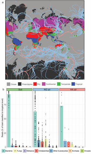
a

3

13

4

14

5

15

6

16

7

17

8

1

11

2

9

18

1210

TropicalOcean Polar/alpine Dry Continental Temperate

b Soil NG air HA air

0

25

50

75

Reads (

% o

f to

tal cla

ssifie

d to k

ingdom

level)

Bacteria Fungi Metazoa Viridiplantae Other Eukaryotas Archaea Viruses

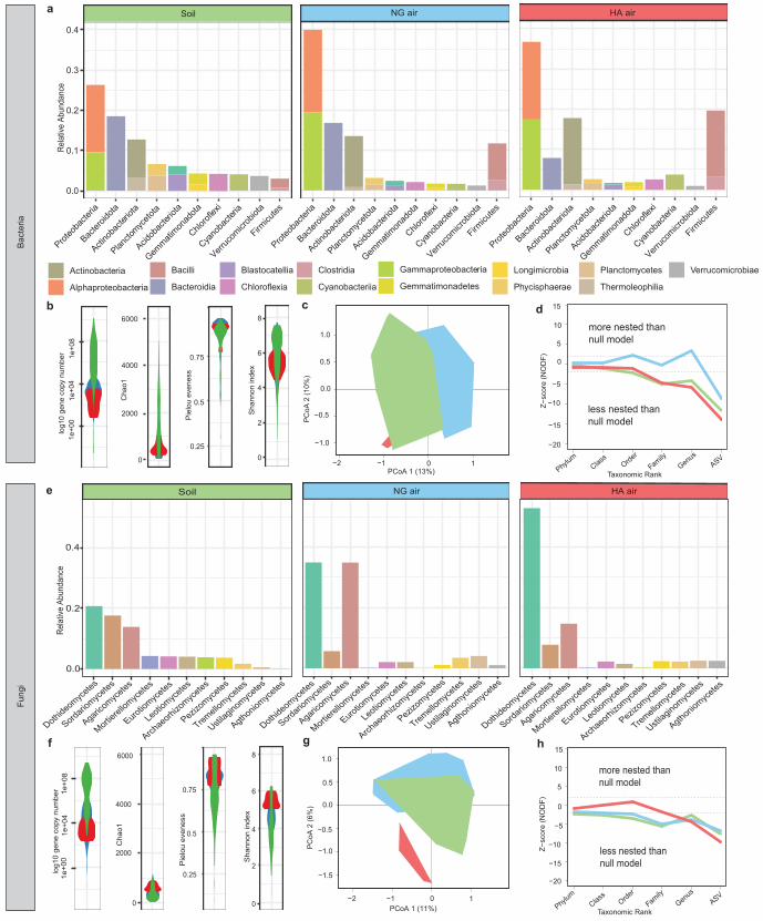
−20

−15

−10

−5

0

5

10

15

Z−sc

ore

(NO

DF)

more nested than null model

less nested than null model

more nested than null model

less nested than null model

Taxonomic RankPhylum

ClassOrder

FamilyGenu

sASV

−20

−15

−10

−5

0

5

10

15

Z−sc

ore

(NO

DF)

Taxonomic RankPhylum

ClassOrde

r

Family

Genus

ASV−2 −1 0 1

−1.5

−1.0

−0.5

0.0

0.5

1.0

PCoA 1 (11%)

PC

oA 2

(6%

)

−2 −1 0 1

−1.0

−0.5

0.0

0.5

1.0

PCoA 1 (13%)

PC

oA 2

(10%

)

Soil

Proteo

bacte

ria

Bacter

oidota

Actino

bacte

riota

Acidob

acter

iota

Planctom

yceto

ta

Chlorof

lexi

Gemmati

monad

ota

Cya

noba

cteria

Verruc

omicr

obiot

a

Firmicu

tes

0.0

0.1

0.2

0.3

0.4

Actinobacteria

Alphaproteobacteria

Bacilli

Bacteroidia

Blastocatellia

Chloroflexia

Clostridia

Cyanobacteriia

Gammaproteobacteria

Gemmatimonadetes

Longimicrobia

Phycisphaerae

Planctomycetes

Thermoleophilia

Verrucomicrobiae

Soil

Dothideomycetes

Sordariomyce

tes

Agaricomyce

tes

Mortierellomyce

tes

Eurotiomyce

tes

Leotiomyce

tes

Archaeorhizo

mycetes

Pezizomyce

tes

Tremellomycetes

Ustilaginomyce

tes

Agthoniomycetes

0.0

0.2

0.4

Rela

tive

Abun

danc

e

a

c d

e

g hf

Bac

teria

Fung

i

Rela

tive

Abun

danc

e

NG air

NG air

HA air

HA air

0

2000

4000

6000

0

2

4

6

8

0.25

0.5

0.75

1e+0

01e

+04

1e+0

8lo

g10

gene

cop

y nu

mbe

r

Cha

o1

Pie

lou

even

ess

Sha

nnon

inde

x

b

0

2000

4000

6000

0.25

0.5

0.75

0

2

4

6

8

1e+0

01e

+04

1e+0

8lo

g10

gene

cop

y nu

mbe

r

Cha

o1

Pie

lou

even

ess

Sha

nnon

inde

xProt

eoba

cteria

Bacter

oidota

Actino

bacte

riota

Acidob

acter

iota

Planctom

yceto

ta

Chlorof

lexi

Gemmati

monad

ota

Cya

noba

cteria

Verruc

omicr

obiot

a

Firmicu

tes

Proteo

bacte

ria

Bacter

oidota

Actino

bacte

riota

Acidob

acter

iota

Planctom

yceto

ta

Chlorof

lexi

Gemmati

monad

ota

Cya

noba

cteria

Verruc

omicr

obiot

a

Firmicu

tes

Dothideomycetes

Sordariomyce

tes

Agaricomyce

tes

Mortierellomyce

tes

Eurotiomyce

tes

Leotiomyce

tes

Archaeorhizo

mycetes

Pezizomyce

tes

Tremellomycetes

Ustilaginomyce

tes

Agthoniomycetes

Dothideomycetes

Sordariomyce

tes

Agaricomyce

tes

Mortierellomyce

tes

Eurotiomyce

tes

Leotiomyce

tes

Archaeorhizo

mycetes

Pezizomyce

tes

Tremellomycetes

Ustilaginomyce

tes

Agthoniomycetes

Soil-NG air NG-HA air Soil-HA air

0.00

0.05

0.10

0.15

0.20

Share

d A

SV

0.00

0.10

0.20

0.30

Share

d A

SV

Sample pairsWithin locationBetween locations

Soil-NG air NG-HA air Soil-HA air

a b 0.12

0.08

0.04

0.0010 17 18 18 2 5 612 11 3 4 1314 1516 9 318 51211 14

Sourc

e c

ontr

ibution

NG air HA air

0.6

0.4

0.2

0.01017 1818 2 56 12 11 3 4 13141516 9 318 512 11 14

Sourc

e c

ontr

ibution

NG air HA air

0.8

8

TropicalOcean Polar/alpine Dry Continental Temperate Phyllosphere

Bacte

ria

Fungi

Cold shock

Oxidative

stress

Sporulation

Starvation

UV repair

Respiration

Carbon

fixation

Nitrogen

fixation

Phototrophy

Trace gas

metabolism

coxL

Fe/FeFe

isoA

isoA/mmoX

pmoA

psaA

psbA

RHO

nifH

rbcL

atpA

ccoN/coxA

cydA

cyoA

nuoF

sdhA/frdA

phrB

uvrB

uvrC

dps

slp

spo0A

msrP

msrQ

cspA/B/G/I

Ocean

Temperate

Dry

Continental

Tropical

Polar/alpine

HA airNG airSoil

Sporu

lation

Cold

sho

ck

Respiration

Oxid

. S

tre

ss

Tra

ce g

as m

et.

Sta

rvation

Photo

trophy

UV

rep

air

C fix

ation

N fix

ation

0

100

1000200

2000

0

100

1000200

2000

0

100

1000200

2000

0

100

1000200

2000

0

100

1000200

2000

0

100

1000200

2000

a b

0 50 >200

Copies/million reads

Soil NG air HA air

Copie

s/m

illio

n r

eads

Loca

tion

latitud

e

Loca

tion

altitud

e

Loca

tion

MAP

Loca

tion

MAT

Trans

it te

mpe

ratu

re

Trans

it RH

Trans

it altitud

e

Trans

it so

lar r

adiatio

n

−0.47−0.36−0.25−0.15−0.040.070.170.280.390.50.6

Respiration

Carbon

fixation

Nitrogen

fixation

Phototrophy

Trace

gas met.

−0.43−0.37−0.32−0.26−0.2

−0.14−0.08−0.020.040.1

0.16Cold

shock

Oxidative

stress

Sporulation

Starvation

UV

repair

−0.5−0.41−0.32−0.24−0.15−0.06

0.020.110.20.290.37Bacteria

abundance

Bacteria

richness

Fungi

abundance

Fungi

richness

Loca

tion

latitud

e

Loca

tion

altitud

e

Loca

tion

MAP

Loca

tion

MAT

0.730.60.460.330.20.07

-0.07-0.2-0.33-0.46-0.6

air soila b

**

*

**

**

**

** **

** ** * *

* **

** ** * *

**

*

**

*

*

*

*

*

*

* *

*

****

*

−0.52−0.43−0.35−0.27−0.19−0.1−0.020.060.140.23

−0.68−0.55−0.43−0.3

−0.17−0.050.080.2

0.330.450.58

0.31

1

Global biogeography of atmospheric microorganisms reflects diverse recruitment and

environmental filtering

Supplementary Information

Stephen D.J. Archer, Kevin C. Lee, Tancredi Caruso, Marcus H.Y. Leung, Xinzhao Tong, Susannah J. Salter,

Graham Hinchliffe, Teruya Maki, Tina Santl-Temkiv, Kimberley A. Warren-Rhodes, Benito Gomez-Silva,

Kevin D. Hyde, Celine J.N. Liu, Antonio Alcami, Dina M. Al Mailem, Jonathan G.Araya, S. Craig Cary, Don

A. Cowan, Jessica Dempsey, Claudia Etchebehere, Batdelger Gantsetseg, Sean Hartery, Mike Harvey, Kazuichi

Hayakawa, Ian Hogg, Mutsoe Inoue, Mayada K. Kansour, Timothy Lawrence, Charles K. Lee, Matthias

Leopold, Christopher P. McKay, Seiya Nagao, Yan Hong Poh, Jean-Baptiste Ramond, Alberto Rastrojo, Toshio

Sekiguchi, Joo Huang Sim, William Stahm, Henry J. Sun, Ning Tang, Bryan Vandenbrink, Craig Walther,

Patrick K.H. Lee, Stephen B. Pointing*

*e-mail: yncpsb@nus.edu.sg

2

Contents

Supplementary methods (page 4)

Table S1 | Globally distributed sampling locations included in the study (page 4)

Supplementary notes on environmental metadata (page 5)

Fig. S1 | Mean transit altitudes for sampled air (page 5)

Fig. S2 | Atmospheric variables encountered by microorganisms during transit to each sampling location

(page 6)

Supplementary notes on sample recovery (page 7)

Fig. S3 | Photographic illustration of terrestrial, marine and aircraft-mounted air sampling (page 8)

Supplementary notes on the use of Null models (page 8)

Fig. S4 | Jaccard network null model for bacterial ASV (page 9)

Fig. S5 | Jaccard network null model for fungal ASV (page 10)

Table S2 | Functional genes targeted in the metagenomics inquiry of air and soil (page 11)

Decontamination of environmental sequence data (page 12)

Fig S6 | Summary of steps taken to minimise contamination during environmental DNA recovery and

sequencing from low biomass air and soil samples (page 12)

Fig. S7 | Sequencing read depth for controls and environmental samples (page 13)

Fig. S8 | Comparison of pre-decontamination taxonomic composition of bacteria in controls and samples

(page 14)

Fig. S9 | Comparison of pre-decontamination taxonomic composition of fungi in controls and samples

(page 15)

Table S3 | Total percentage of sequenced reads removed from each step of the decontamination process.

(page 16)

Fig. S10 | Relationship between soil biomass and bacterial reads retained post-filtering (page 17)

Fig. S11 | Relationship between soil biomass and fungal reads retained post-filtering (page 18)

Fig S12 | Rarefaction curves for post-filtered amplicon sequence data (page 19)

Fig S13 | Rarefaction curves for post-filtered metagenomes (page 20)

Fig S14 | Taxonomic identity of reads removed during the decontamination process (page 20)

Fig. S15 | Post-decontamination check for residual contaminants (page 22)

Fig. S16 | Taxonomic composition of potential residual contaminants (page 23)

Fig S17 | Evaluation for batch effects and temporal auto-correlation in samples (page 25)

3

Fig. S18 | Taxonomic identity of reads removed during the decontamination process by location (page

26)

Fig. S19 | Comparison of bacterial diversity estimation pre- and post-decontamination (page 27)

Fig. S20 | Comparison of fungal diversity estimation pre- and post-decontamination (page 27)

Fig. S21 | Comparison of community resemblance pre- and post-decontamination (page 28)

Supplementary results (page 29)

Fig. S22 | Global patterns in alpha diversity for bacteria and fungi in air and soil (page 29)

Fig. S23 | Comparison of diversity estimation using shotgun metagenomics and amplicon sequencing of

air and soil (page 30)

Table S4 | The effect of habitat and location on structure of bacterial and fungal assemblages (page 31)

Fig. S24 | Dissimilarity of assemblages by habitat type and location (page 32)

Fig. S25 | Phylogenetic distance of assemblages by habitat type and location (page 33)

Fig. S26 | Global-scale distance decay plots for bacteria and fungi in air and soil (page 34)

Fig. S27 | Null model networks for bacterial and fungal assemblages in air and soil (page 35)

Fig. S28 | Taxonomic composition of bacterial and fungal assemblages in air and underlying soil (page

36)

Fig. S29 | Co-occurrence of bacterial and fungal taxa in globally distributed air and soil (page 37)

Table S5 | List of bacterial genera prevalent in ≥ 50% of soil and/or air samples (page 38)

Table S6 | List of fungal genera prevalent in ≥ 50% of soil and/or air samples (page 39)

Fig. S30 | Source contribution to observed diversity in air (page 40)

Fig. S31 | Functional metagenomics profiling of targeted stress-response and metabolic genes by habitat

type (page 41)

Supplementary references (page 42)

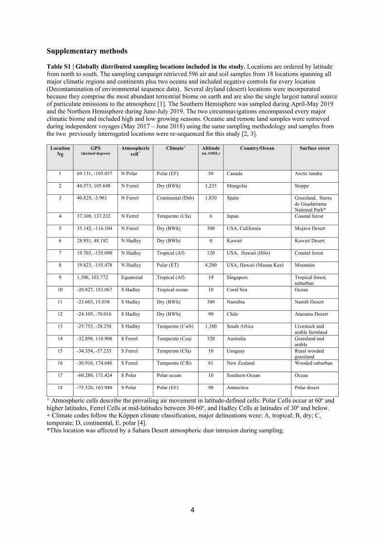
4

Supplementary methods

Table S1 | Globally distributed sampling locations included in the study. Locations are ordered by latitude

from north to south. The sampling campaign retrieved 596 air and soil samples from 18 locations spanning all

major climatic regions and continents plus two oceans and included negative controls for every location

(Decontamination of environmental sequence data). Several dryland (desert) locations were incorporated

because they comprise the most abundant terrestrial biome on earth and are also the single largest natural source

of particulate emissions to the atmosphere [1]. The Southern Hemisphere was sampled during April-May 2019

and the Northern Hemisphere during June-July 2019. The two circumnavigations encompassed every major

climatic biome and included high and low growing seasons. Oceanic and remote land samples were retrieved

during independent voyages (May 2017 – June 2018) using the same sampling methodology and samples from

the two previously interrogated locations were re-sequenced for this study [2, 3].

Location

No

GPS (decimal degrees)

Atmospheric

cell^

Climate+ Altitude (m AMSL)

Country/Ocean Surface cover

1

69.131, -105.057 N Polar Polar (EF) 50 Canada Arctic tundra

2

44.573, 105.648 N Ferrel Dry (BWk) 1,235 Mongolia Steppe

3

40.825, -3.961 N Ferrel Continental (Dsb) 1,830 Spain Grassland, Sierra

de Guadarrama

National Park*

4

37.308, 137.232 N Ferrel Temperate (Cfa) 6 Japan Coastal forest

5

35.142, -116.104 N Ferrel Dry (BWk) 300 USA, California Mojave Desert

6

28.951, 48.192 N Hadley Dry (BWh) 0 Kuwait Kuwait Desert

7

19.703, -155.090 N Hadley Tropical (Af) 120 USA, Hawaii (Hilo) Coastal forest

8

19.823, -155.478 N Hadley Polar (ET) 4,200 USA, Hawaii (Mauna Kea) Mountain

9

1.306, 103.772 Equatorial Tropical (Af) 19 Singapore Tropical forest,

suburban

10

-20.827, 153.067 S Hadley Tropical ocean 10 Coral Sea Ocean

11

-23.603, 15.038 S Hadley Dry (BWh) 380 Namibia Namib Desert

12

-24.105, -70.016 S Hadley Dry (BWh) 90 Chile Atacama Desert

13

-25.753, -28.258 S Hadley Temperate (Cwb) 1,380 South Africa Livestock and

arable farmland

14

-32.898, 116.906 S Ferrel Temperate (Csa) 320 Australia Grassland and

arable

15

-34.354, -57.235 S Ferrel Temperate (Cfa) 10 Uruguay Rural wooded

grassland

16

-36.916, 174.646 S Ferrel Temperate (Cfb) 61 New Zealand Wooded suburban

17

-60.288, 171.424 S Polar Polar ocean 10 Southern Ocean Ocean

18

-75.520, 163.949 S Polar Polar (EF) 98 Antarctica Polar desert

^ Atmospheric cells describe the prevailing air movement in latitude-defined cells: Polar Cells occur at 60o and

higher latitudes, Ferrel Cells at mid-latitudes between 30-60o, and Hadley Cells at latitudes of 30o and below.

+ Climate codes follow the Kӧppen climate classification, major delineations were: A, tropical; B, dry; C,

temperate; D, continental, E, polar [4].

*This location was affected by a Sahara Desert atmospheric dust intrusion during sampling.

5

Supplementary notes on environmental metadata

Long-term macroclimate variables for each sampling location (Table S1) were retrieved from public databases:

mean annual precipitation and mean annual temperature [5], Kӧppen-Geiger climate classifications [6], growing

season that defined the time period when photoautotrophy can occur [7]. Other local variables were recorded

using handheld devices: Temperature (°C), relative humidity (%), wind speed (m/S) and wind direction (Kestrel

Meters, USA); Particulate matter (PM 2.5 and PM 10.0) (HoldPeak, China). Full metadata for each sampling

location and event are available upon request at http://atmospheric-microbiome.com/. In order to identify back trajectory and environmental variables encountered by microorganisms during their transit in air towards each

sampling location, we obtained data from the NOAA HYSPLIT-model, and long-range trajectories and abiotic

variables were estimated using the NOAA Global Data Assimilation System (GDAS) [8]. The depths of the

atmospheric boundary layer (mixing depths) were calculated from meteorological fields of the GDAS model

that was used to calculate the back trajectories (Fig. S1). Fourteen day back trajectories of air masses for each

sampling time were generated because this is the estimated maximum residence time for microorganisms in the

troposphere (Fig. S2) [9]. The following variables were calculated at intervals along each tropospheric transport

path from the HYSPLIT models: altitude (m above ground level, AGL), wind speed (m/S), direction,

temperature (oC), Relative humidity (%), solar irradiance (W/m2), precipitation events, and transit duration over

land or ocean surface (Fig. S2). Data was processed using ArcGIS Pro, version 2.6 (https:/www.esri.com).

Points were plotted on WGS 1984 Web Mercator coordinate system with date line wrapping and climate mapping at 1km resolution [6].

Fig. S1 | Mean transit altitudes for sampled air. Blue denotes near-ground sampling (NG air), red denotes

high-altitude aircraft sampling above the atmospheric boundary layer (HA air), bar indicates depth of the

atmospheric boundary layer. Locations: 1, Canada; 2, Mongolia; 3, Spain; 4, Japan; 5, California, USA; 6,

Kuwait; 7, Hilo, Hawaii, USA; 8; Mauna Kea, Hawaii, USA; 9, Singapore; 10, Coral Sea; 11, Namibia; 12,

Chile; 13, South Africa; 14, Australia; 15, Uruguay; 16, New Zealand; 17, Southern Ocean; 18, Antarctica. All

altitudes and depths are shown as metres above local ground level (AGL).

6

Fig. S2 | Atmospheric variables encountered by microorganisms during transit to each sampling location.

a, Temperature. b, Solar flux. c, Relative humidity. d, Transit over land/ocean. e, Transit altitude. f, Transit

velocity.

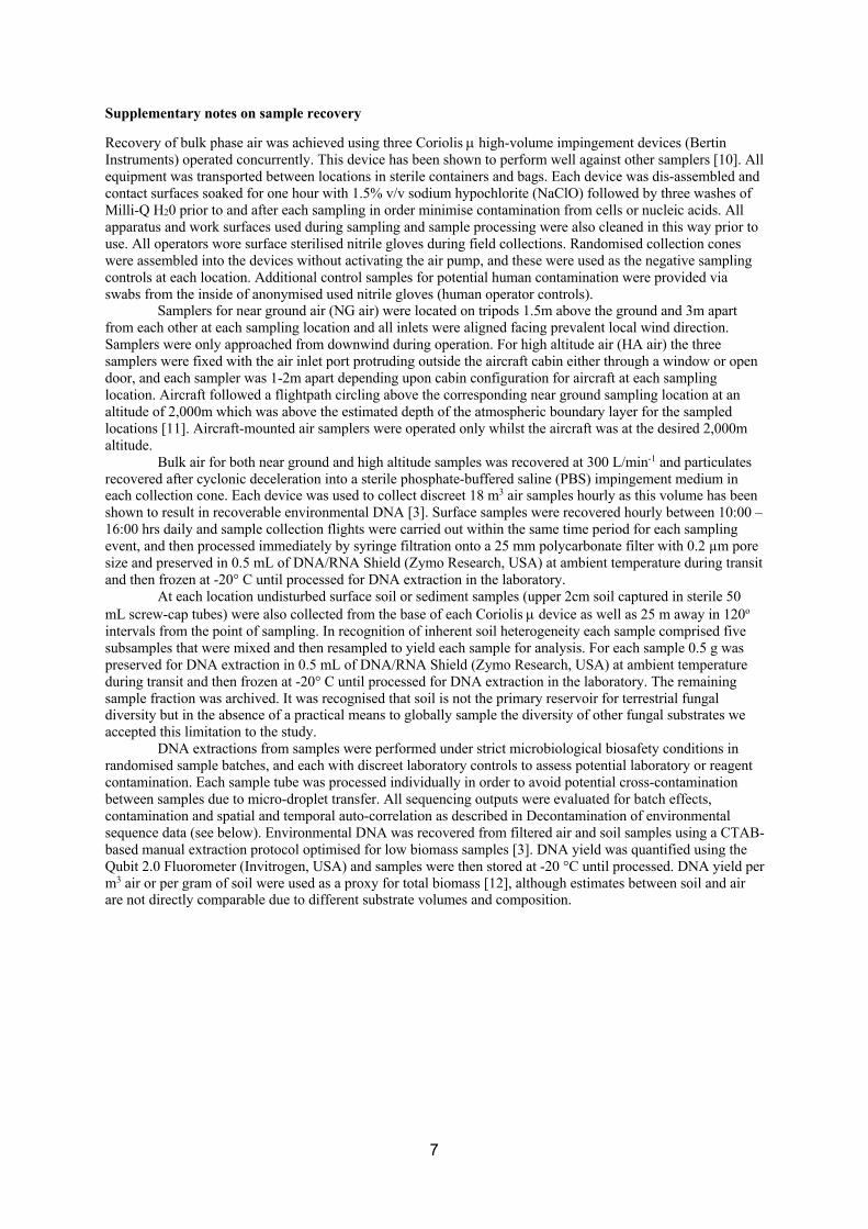
7

Supplementary notes on sample recovery

Recovery of bulk phase air was achieved using three Coriolis µ high-volume impingement devices (Bertin

Instruments) operated concurrently. This device has been shown to perform well against other samplers [10]. All

equipment was transported between locations in sterile containers and bags. Each device was dis-assembled and

contact surfaces soaked for one hour with 1.5% v/v sodium hypochlorite (NaClO) followed by three washes of

Milli-Q H20 prior to and after each sampling in order minimise contamination from cells or nucleic acids. All

apparatus and work surfaces used during sampling and sample processing were also cleaned in this way prior to

use. All operators wore surface sterilised nitrile gloves during field collections. Randomised collection cones

were assembled into the devices without activating the air pump, and these were used as the negative sampling

controls at each location. Additional control samples for potential human contamination were provided via

swabs from the inside of anonymised used nitrile gloves (human operator controls). Samplers for near ground air (NG air) were located on tripods 1.5m above the ground and 3m apart

from each other at each sampling location and all inlets were aligned facing prevalent local wind direction.

Samplers were only approached from downwind during operation. For high altitude air (HA air) the three

samplers were fixed with the air inlet port protruding outside the aircraft cabin either through a window or open

door, and each sampler was 1-2m apart depending upon cabin configuration for aircraft at each sampling

location. Aircraft followed a flightpath circling above the corresponding near ground sampling location at an

altitude of 2,000m which was above the estimated depth of the atmospheric boundary layer for the sampled

locations [11]. Aircraft-mounted air samplers were operated only whilst the aircraft was at the desired 2,000m

altitude.

Bulk air for both near ground and high altitude samples was recovered at 300 L/min-1 and particulates

recovered after cyclonic deceleration into a sterile phosphate-buffered saline (PBS) impingement medium in each collection cone. Each device was used to collect discreet 18 m3 air samples hourly as this volume has been

shown to result in recoverable environmental DNA [3]. Surface samples were recovered hourly between 10:00 –

16:00 hrs daily and sample collection flights were carried out within the same time period for each sampling

event, and then processed immediately by syringe filtration onto a 25 mm polycarbonate filter with 0.2 µm pore

size and preserved in 0.5 mL of DNA/RNA Shield (Zymo Research, USA) at ambient temperature during transit

and then frozen at -20° C until processed for DNA extraction in the laboratory.

At each location undisturbed surface soil or sediment samples (upper 2cm soil captured in sterile 50

mL screw-cap tubes) were also collected from the base of each Coriolis µ device as well as 25 m away in 120o

intervals from the point of sampling. In recognition of inherent soil heterogeneity each sample comprised five

subsamples that were mixed and then resampled to yield each sample for analysis. For each sample 0.5 g was

preserved for DNA extraction in 0.5 mL of DNA/RNA Shield (Zymo Research, USA) at ambient temperature

during transit and then frozen at -20° C until processed for DNA extraction in the laboratory. The remaining

sample fraction was archived. It was recognised that soil is not the primary reservoir for terrestrial fungal diversity but in the absence of a practical means to globally sample the diversity of other fungal substrates we

accepted this limitation to the study.

DNA extractions from samples were performed under strict microbiological biosafety conditions in

randomised sample batches, and each with discreet laboratory controls to assess potential laboratory or reagent

contamination. Each sample tube was processed individually in order to avoid potential cross-contamination

between samples due to micro-droplet transfer. All sequencing outputs were evaluated for batch effects,

contamination and spatial and temporal auto-correlation as described in Decontamination of environmental

sequence data (see below). Environmental DNA was recovered from filtered air and soil samples using a CTAB-

based manual extraction protocol optimised for low biomass samples [3]. DNA yield was quantified using the

Qubit 2.0 Fluorometer (Invitrogen, USA) and samples were then stored at -20 °C until processed. DNA yield per

m3 air or per gram of soil were used as a proxy for total biomass [12], although estimates between soil and air are not directly comparable due to different substrate volumes and composition.

8

Fig. S3 | Photographic illustration of terrestrial, marine and aircraft-mounted air sampling. Indicative

images of air sampling setup at a, temperate, b, desert, c, marine, and d, high-altitude aircraft sampling.

Supplementary notes on use of Null models

Models

Null models are widely used by ecologists to detect non-random patterns in data matrices These models

generally require a randomization of observed data subjected to some constraints. The constraints should reflect

the hypotheses under investigation [13–15]. The typical data matrix analysed by ecologists are species by site

tables and tables that represent interactions between different groups of species (for example plant-pollinator or plant-root symbiont networks). Classical ecological null models are constructed by constrained permutations,

which usually fix some general property of the data matrix such as the column or row margins [15–17]. A

metric quantifying the pattern under investigation is then calculated both on the observed data matrix and the

randomly generated matrices. Using the logic of null models, the difference between the observed metrics and

the metrics in the randomised null matrices is expressed as the z-score of the metric, say metric 𝑋, as:

𝑧! =𝑋(𝑶) − ⟨𝑋⟩

𝜎(𝑋) = 𝑋∗ − ⟨𝑋⟩𝜎(𝑋)

Where O is the observed data matrix, 𝑋∗is the observed value of the metric and ⟨𝑋⟩ and 𝜎(𝑋) are the expected

value and standard deviation in the ensemble of the permuted matrices. If ⟨𝑋⟩ and 𝜎(𝑋) describe a normal

distribution, the probability of observing a difference beyond two standard deviations just by chance would be

roughly 0.05, but if the distribution is not normal an operational p-value < 0.05 can be calculated following

classical null modelling [13]. As explained in the main methods, we did not use permutations of the raw data to

construct our null models. The reason is that producing a large number of randomly rewired matrices using

permutations leads to a set of biased null model matrices, if the original matrix is heterogeneous (e.g. some taxa

are much more widespread than others) and sparse [18, 19]. Local randomization algorithms risk sampling the set

of null, random matrices non-uniformly, which means that the estimates of the metrics measured on the data

matrix is not guaranteed to correspond to the correct theoretical expectation. Given all these issues, which would likely affect a classical null model analysis of our data set, we used the so-called network canonical ensemble, a

model belonging to the set of methods known as the statistical mechanics of network. The most complete reference

for our approach is in the book by Squartini & Garlaschelli 2017 [20]. Briefly, we interpreted the taxon by location

data matrix as a binary bipartite network that describes the occurrence of each taxon at each location. We used

the number of taxa at each location or, conversely, the number of locations in which each taxon was found as the

constraining vector for the construction of the null model ensemble. The null model matrices will thus be fully

random in terms of which taxon is found at each location, which is central to hour hypothesis of a non-randomly

structured air microbiome. At the same time, the number of taxa per location and also the number of locations in

which each taxon is found is, on average, the same in the null models and in the observed matrices. This is

a)

c)

d)b)

9

important, because it means that deviations of observed data from the null models will be affected solely by the

taxonomic composition of the assemblage. As it can be easily shown following the derivations [20], the

Hamiltonian of the graph corresponding to our model would then be

H(𝐀, 𝛉) =0θ#k#(𝐀)#

=00(θ# + θ#)a#$$%##

for a general binary matrix, and the probability distribution of each occurrence in the matrix

P(𝐀|𝛉) =77p#$

&!"

$%#

91 − p#$;'(&!"#

. This solution can easily be reparametrized to describe a binary bipartite graph [21]. The probability distribution

P(𝐀|𝛉) is the correct (i.e. it maximises entropy) probability distribution for each taxon randomly occurring in

each location, subject to the constraints given by the number of locations in which that taxon can be found, and

the number of taxa found in each location. The parameters of the distribution can be estimated using maximum likelihood methods [22] (described in the Methods). The probability distribution is then sampled [23], to generate

the desired number of randomised matrices (we sampled 999 matrices) and construct the null model. As the

probability distribution is analytically derived for each of the three types of samples we analysed (soil, near ground

and high elevation air), each type of sample (soil, NG air and HA air) has its own baseline or null model.

Metrics

The metrics we tested in the null models were NODF, a metric of nestedness, and the Jaccard index. There is a

vast, and often lively debated literature on the property of nestedness. Nested pattern have been defined as

(quote) “[nested patterns] are those in which the species composition of small assemblages is a nested subset of

larger assemblage” [24]. This applies also to randomly assembled communities and so a null model is needed to test whether nestedness pattern are not random. Assume the microbial composition at each location is

completely random and just reflects recruitment of the most abundant taxa from the regional pool. Then, any

local community that randomly recruits a relatively small number of taxa will form a subset of the local

communities that randomly happen to recruit a relatively large number of taxa. However, if different groups of

local communities or, also, individual local communities, are characterised by a particular and unique taxonomic

composition, with some taxa that specifically occur only at certain locations and others that occur at other

locations, observed nestedness will be much lower than expected under a null model that fully randomise taxa

composition.

Our second metrics, the Jaccard index on presence/absence data, quantifies pairwise community

dissimilarity. The higher the index the lower the number of taxa shared by the two compared locations. One can

thus calculate the average dissimilarity of a taxon by location matrix, which we did both for the observed and

null model matrices. Our results (Fig. 2) showed that bacterial (Fig. S4) and fungal communities (Fig. S5) in air were more dissimilar than expected under the null model. Fungi in soil showed the same difference. Instead,

bacteria in soil were more similar than expected under the null model.

Fig. S4 | Jaccard network null model for bacterial ASVs.

10

Fig. S5 | Jaccard network null model for fungal ASVs.

There are several possible explanations for convergence and divergence of taxonomic composition relative to

the baseline provided by a stochastic null model (e.g. [25–29]). Soil appeared to have “homogenised” ASVs and

also at higher rank community composition (not shown) relative to the null model. This could be due to

selection forces such as environmental filtering combined with limited dispersal, as discussed in the main text.

In contrast, Air made ASVs and also higher rank taxa composition more heterogeneous than in the null model.

This type of compositional divergence, too, can be due to selective forces but with the environmental conditions

of the locations varying to a large extent between locations, which diversifies the composition of communities across locations. The explanations we are offering for these patterns of compositional dissimilarity observed in

air and soil remain hypotheses to be tested in the future but the Jaccard pattern, together with NODF

demonstrates the non-random structure of the air microbiome in terms of the distribution of taxa across the

network of locations of this study.

11

Table S2 | Functional genes targeted in the metagenomics inquiry of air and soil. A suite of respiratory

genes was used as a general marker of potential for metabolically active taxa, and targeted metabolic and stress

response genes were selected based upon substrates and stressors encountered in the atmospheric habitat.

Trait Protein Gene

Respiration ATP synthase atpA

Cytochrome cbb3 oxidase ccoN

Cytochrome aa3 oxidase coxA

Cytochrome bd oxidase cydA

Cytochrome bo3 oxidase cyoA

NADH-ubiquinone oxidoreductase subunit F nuoF

Succinate dehydrogenase/fumarate reductase sdhA/frdA

Carbon fixation Ribulose 1,5-bisphosphate carboxylase/oxygenase rbcL

Nitrogen fixation Nitrogenase nifH

Phototrophy Photosystem I reaction centre protein psaA

Photosystem II reaction centre protein psbA

Microbial rhodopsin RHO

Atmospheric trace gas metabolism (carbon monoxide, hydrogen, methane,

isoprene)

Aerobic carbon monoxide dehydrogenase coxL

Hydrogenase Fe

Hydrogenase FeFe

Isoprene oxidation gene isoA/mmoX

Soluble methane monooxygenase mmoX

Particulate methane monooxygenase pmoA

cold-shock Cold shock protein A cspA

Cold shock protein B cspB

Cold shock protein G cspG

Cold shock protein I cspI

Oxidative stress Protein-methionine sulfoxide reductase msrP

Protein-methionine sulfoxide reductase msrQ

Sporulation Sporulation protein 0A spo0A

Starvation/stationary phase DNA-protection during starvation protein dps

Outer membrane protein slp

UV response/repair Deoxyribodipyrimidine photo-lyase phrB

UvrABC system protein A uvrA

UvrABC system protein B uvrB

UvrABC system protein C uvrC

Ice nucleation Ice nucleation protein A inaA

Ice nucleation protein X inaX

Ice nucleation protein W inaW

Ice nucleation protein Z inaZ

12

Decontamination of environmental sequence data

Here we present supporting evidence to demonstrate our decontamination pipeline resulted in effective removal

of contaminants and did not adversely impact the observed ecological patterns for our data. Our approach to

decontamination adopted and fully reports a thorough multi-step decontamination protocol as per recommended

best practice [30–32]. The decontamination of our sequence data was an integral part of our wider approach to

careful sampling of ultra-low biomass atmospheric samples and soils (Fig. S6).

Fig S6 | Summary of steps taken to minimise contamination during environmental DNA recovery and

sequencing from low biomass air and soil samples. QC denotes quality control, ASV denotes amplicon

sequence variant, NTU denotes nearest taxonomic unit used for taxa assignment from metagenomes.

Our close attention to careful field sampling and laboratory workflow resulted in very low read numbers for our

control samples compared to environmental samples (Fig. S7). A very small number of 16S rRNA gene

sequencing controls (n = 3) with higher reads did not identify significantly more ASVs for removal, rather they

largely comprised higher read numbers of ASVs that also occurred in other controls. We regard this as an

important part of the heterogeneity encountered in environmental microbiology and so we retained these

controls in our decontamination pipeline. Due to our careful attention to randomization and replication the few

controls with higher reads did not impact the ecological patterns presented for the filtered data.

13

Fig. S7 | Sequencing read depth for controls and environmental samples. a, Bacteria read depth (controls: n

= 35; samples: n = 529). b, Fungi read depth (controls: n = 35; samples: n = 444). c, Metagenomes read depth

for controls (n = 3, pooled by type from 35 independent control samples) and samples (n = 120). Boxplots

indicate median (line) and interquartile range (boxes).

We report the removal of reads at each of the decontamination steps for our amplicon sequence data as per

recommended best practice (Table S3) [31]. Sequencing studies of dilution series for mock communities have

shown that there is an unavoidable increase in contaminant signal as starting template decreases [33]. This and

other studies, e.g. [30], indicate that the percentage of contaminants detected during dilution series to obtain

template DNA levels similar to those in our study were comparable or higher (approx. 50-80% in mock

communities) to those we observed for our environmental samples, thus supporting that the level of

contaminants we encountered was not unexpectedly high for the ultra-low biomass habitats being interrogated.

Furthermore, the proportion of reads removed from our dataset is consistent with the range in published reports

for other ultra-low biomass environmental studies where numbers have been disclosed, i.e. Sheik et al. (2018)

concluded approximately 27% of OTUs in deep biosphere samples were contaminants [34], Els et al. (2019) removed 40% of amplicon OTUs during decontamination [35], Kiledal et al. (2021) removed 85% of amplicon

reads during decontamination [36].

We report the diversity of ASV removed at each stage of our decontamination process (Fig. S9).

Untargeted sequence removal included reads affiliated with chloroplasts, mitochondria and other non-target

organisms. The R package decontam was applied using a stringent statistical threshold for frequency (0.1)

and/or prevalence (0.5). Control removal included any taxa occurring in any of the field blanks, laboratory

blanks or swabs of human operator gloves being filtered from all samples. Finally, the filtering of named genera

targeted any remaining taxa commonly reported as human-associated contaminants (n = 21 genera) in

published meta-analyses of ultra-low biomass microbiomes [30, 31].

14

Fig. S8 | Comparison of pre-decontamination taxonomic composition of bacteria in controls and

samples. Bubble plots illustrating genus-level taxonomic composition of bacteria in controls and samples

prior to decontamination workflow. Bubble sizes indicate relative abundance. Note that absolute

abundance varied due to lower reads in controls versus samples (Fig. S7). Values are the mean of all

replicates for any given treatment. NG air = near-ground air, HA air = high-altitude air.

15

Fig. S9 Comparison of pre-decontamination taxonomic composition of bacteria in controls and

samples. Bubble plots illustrating genus-level taxonomic composition of fungi in controls and samples

prior to decontamination workflow. Bubble sizes indicate relative abundance. Note that absolute

abundance varied due to lower reads in controls versus samples (Fig. S7). Values are the mean of all

replicates for any given treatment. NG air = near-ground air, HA air = high altitude air.

16

Table S3 | Total percentage of sequenced reads removed from each step of the decontamination process.

NG air denotes near-ground air and HA air denotes high-altitude air.

16S rRNA gene sequencing decontamination (% of total reads removed from previous step)

Soil NG air HA air

Untargeted (%) 0.71 10.84 6.35

Decontam (%)+ 9.67 21.65 21.24

Control removal (%)# 4.99 9.57 8.43

Genus-level filtering (%)^ 0.22 0.9 1.58

Total removed (%) = 15.58 42.98 37.60

ITS sequencing decontamination (% of total reads removed from previous step)

Soil NG air HA air

Untargeted (%) 1.0 0.07 0.05

Decontam (%)+ 23.28 42.98 51.25

Control removal (%)# 3.24 12.39 10.09

Genus-level filtering (%)^ 0.13 0.06 0.03

Total removed (%)@ 27.55 55.49 61.44

+ The removal of suspiciously frequent and/or prevalent ASVs using the R package decontam resulted in higher

numbers of removed ASVs from near-ground air and high-altitude air samples due to the ultra-low biomass of

samples and unavoidable increase in contaminant signal [30, 31].

# ASVs occurring in any of the field sampling controls, human operator controls or laboratory reagent controls

were removed from all samples regardless of whether they were encountered in location-specific or habitat-

specific controls where a given sample was recovered.

^ Whilst our decontam and control removal steps removed most common human and reagent contaminants, we

also applied an additional subtractive filter to remove any remaining suspected human-associated contaminants.

We targeted the following bacterial genera: Bacteroides, Bifidobacterium, Corynebacterium,

Cutibacterium/Propionibacterium, Escherichia, Faecalibacterium, Haemophilus, Klebsiella, Lactobacillus,

Listeria, Moraxella, Neisseria, Porphyromonas, Prevotella, Shigella, Salmonella, Staphylococcus,

Streptococcus and Veillonella. We also removed ASV affiliating with the human-associated fungal genera

Candida and Malassezia. We acknowledge that some of these genera, e.g. Klebsiella, Lactobacillus, Listeria,

Candida (together approx. 0.1% reads in our study) may also support environmental taxa but we chose to take a

cautious approach and remove all ASVs in the genus because most of these ASVs in our study affiliated to

human-associated taxa or it was uncertain from database metadata if they were genuine environmental taxa.

= Soils were highly heterogenous and soil biomass was positively correlated with retained reads post-filtering. In

all but the most extreme desert mineral soils the average occurrence of potential contaminants was ~1% of

bacterial and ~5% of fungal quality-filtered reads (Figs S10, S11).

@ Relatively high read removal for ITS reads may in part reflect the nature of fungal spore emission and this is

impossible to deconvolute from the algorithm for suspicious frequency/prevalence in decontamination software.

In order to be cautious in our approach, we report the diversity of all removed taxa so these data are not lost

from the study.

A similarly rigorous process was applied to our metagenomes:

Shotgun metagenome decontamination (% of total reads removed from previous step)

Soil NG air HA air

Contaminant contig mapping (%) 4.86 5.33 4.21

Decontam (Bacteria) (%) 0.29 1.03 1.5

Genus-level filtering (Bacteria) (%) 0.61 1.56 1.13

Decontam (Fungi) (%) 0.069 0.47 1.52

Genus-level filtering (Fungi) (%) 0.0002 0.0008 0.014

Total removed(%) 5.83 8.39 8.38

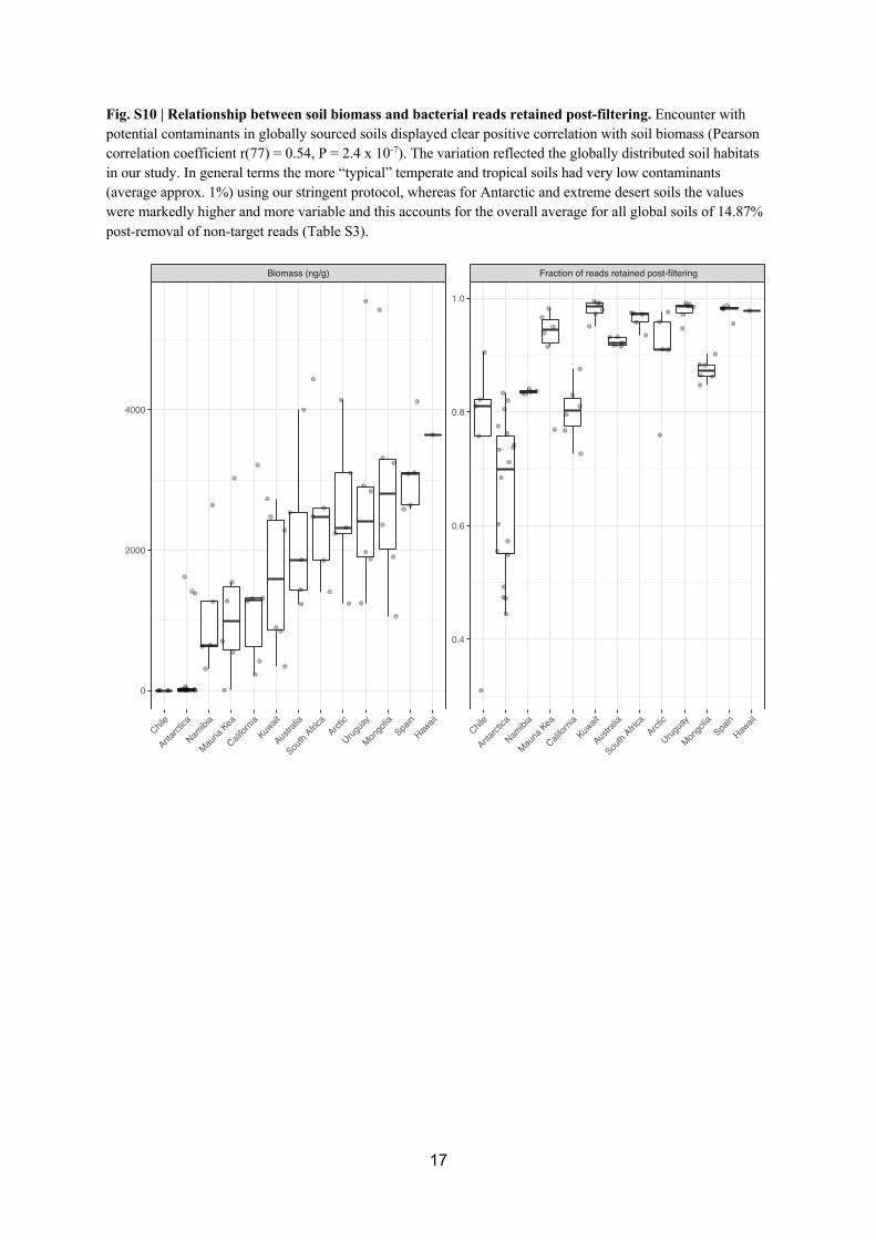
17

Fig. S10 | Relationship between soil biomass and bacterial reads retained post-filtering. Encounter with

potential contaminants in globally sourced soils displayed clear positive correlation with soil biomass (Pearson

correlation coefficient r(77) = 0.54, P = 2.4 x 10-7). The variation reflected the globally distributed soil habitats

in our study. In general terms the more “typical” temperate and tropical soils had very low contaminants

(average approx. 1%) using our stringent protocol, whereas for Antarctic and extreme desert soils the values

were markedly higher and more variable and this accounts for the overall average for all global soils of 14.87%

post-removal of non-target reads (Table S3).

Biomass (ng/g) Fraction of reads retained post-filtering

Chile

Antar

ctica

Nam

ibia

Mau

na K

ea

Califo

rnia

Kuwait

Austra

lia

South

Afri

ca

Arctic

Uru

guay

Mon

golia

Spain

Haw

aii

Chile

Antar

ctica

Nam

ibia

Mau

na K

ea

Califo

rnia

Kuwait

Austra

lia

South

Afri

ca

Arctic

Uru

guay

Mon

golia

Spain

Haw

aii

0.4

0.6

0.8

1.0

0

2000

4000

18

Fig. S11 | Relationship between soil biomass and fungal reads retained post-filtering. Encounter with

potential contaminants displayed clear positive correlation with soil biomass (Pearson correlation coefficient

r(68) = 0.65, P = 1.18 x 10-9). The variation reflected the globally distributed soil habitats in our study. In

general terms the more “typical” temperate and tropical soils had very low contaminants (average approx. 5%

for fungi) using our stringent protocol, whereas for Antarctic and extreme desert soils the values were markedly

higher and more variable and this accounts for the overall average for all global soils of 26.55% for fungi post-

removal of non-target reads (Table S3).

Biomass (ng/g) Fraction of reads retained post−filtering

Chile

Antar

ctica

Califo

rnia

Mau

na K

ea

Nam

ibia

Kuwait

Austra

lia

Uru

guay

Mon

golia

Arctic

South

Afri

ca

Spain

Haw

aii

Chile

Antar

ctica

Califo

rnia

Mau

na K

ea

Nam

ibia

Kuwait

Austra

lia

Uru

guay

Mon

golia

Arctic

South

Afri

ca

Spain

Haw

aii

0.4

0.6

0.8

1.0

0

2000

4000

19

Fig S12 | Rarefaction curves for amplicon sequence data. a, Bacteria (soil (n = 79), near-ground air (NG air)

(n = 437) and high-altitude air (HA air)). b, Fungi (soil (n = 70), near-ground air (NG air, n = 363) and high-

altitude air (HA air, n = 11)). Sampling curves are shown for sequence data after subtractive filtering by the

comprehensive decontamination steps. The number of reads for bacteria, after filtering (final data) was: Min:

1,303, Median: 18,877, Mean: 23,114, Max: 174,577; and for fungi, after filtering (final data) was: Min: 1,106, Median: 14,238, Mean: 18,187, Max: 116,859.

20

Fig S13 | Rarefaction curves for Metagenomes (n = 120). NG air denotes near-ground air and HA air denotes

high-altitude air.

Fig. S14 | Taxonomic identity of reads removed during the decontamination process. Taxonomic

composition of removed reads for the 10 most abundant classes at each decontamination step (a) and overall (b)

bacterial amplicon data; Taxonomic composition of removed reads for the 10 most abundant classes at each

decontamination step (c) and overall (d) fungal amplicon data. Note: Cyanobacteria removed reads affiliated to

chloroplasts, a portion of Alphaproteobacteria reads removed affiliated to mitochondria.

21

We next performed a post-hoc analysis of our filtered dataset after decontamination to estimate the effectiveness

of the multi-step subtractive filtering process and identify any remaining ASVs that may represent potential

residual contaminants, as well as identify any evidence for cross-contamination between sample types. In order

to focus on unequivocal contamination events, we subsampled the data to 1000 reads per sample and removed

taxa that were present in fewer than 10 samples. FastSpar correlation scores and their P values were determined for genus-level taxa and then heatmaps were used to visualise clusters indicative of potential artefacts (Fig S15).

Next, taxonomic composition of each cluster were checked for frequency and prevalence of the taxa throughout

the dataset. For a cluster to be identified as an artefact suitable for subtraction we applied the following criteria:

i) It should align with metadata such as processing batch, sequencing batch, or reagent lot numbers, ii) It should

be implausibly consistent between samples, for example if it spans multiple ecological locations, iii) it should be

extremely rare beyond the artefact itself.

The analysis revealed a small number of clusters in the bacterial and fungal datasets and weak

correlation blocks overall. This indicates a low possibility of exogenous contaminant since taxa arising from a

common source would correlate more strongly than real ecological associations. There was no evidence for

batch effects (i.e. correlation blocks did not match up with processing batch, sequencing batch, or reagent lot

numbers) but a small number of genera displayed clustering indicative of potential residual contamination. A

cluster comprising Ampullimonas, Rhizobacter, Tardiphaga, Variovorax, and unclassified Methylophilaceae appeared to form a tightly correlating pattern that was not tied to geographic origin and so they are likely to be

residual contaminants. Additional weak clusters yielded inconclusive evidence for potential residual

contamination from Acidovorax, Bradyrhizobium Pseudomonas, Ralstonia, and Sphingomonas. The latter

genera contain ASVs that were removed during our decontamination steps but they also contain known

environmental taxa and so removing them at genus level was deemed imprudent. For the fungi a single

correlation block affecting 88 samples was identified as worthy of further scrutiny, but since these samples all

originated from marine and maritime locations in the southern hemisphere it was concluded this likely

represented a valid separation from other samples geographically and by ocean-land site separation.

We identified all ASVs in our filtered bacterial dataset that affiliated within the genera identified as

potentially suspicious from this analysis (Fig. S16). Most of these formed a very low percentage of overall

diversity with the exception of Ralstonia, where a small number of ASVs occurred with higher frequency in some high-altitude air samples. In view of the overall low number of potential residual contaminants, that they

affiliated with genera that have known environmental taxa as well as commonly encountered contaminants, and

in order to preserve the clear step-wise decontamination process was applied identically across samples; we

chose not to perform further removal of these ASVs, although we report their taxonomic affiliation so that this

can be used to nuance our data. The filtered fungal dataset revealed no potential residual contaminants.

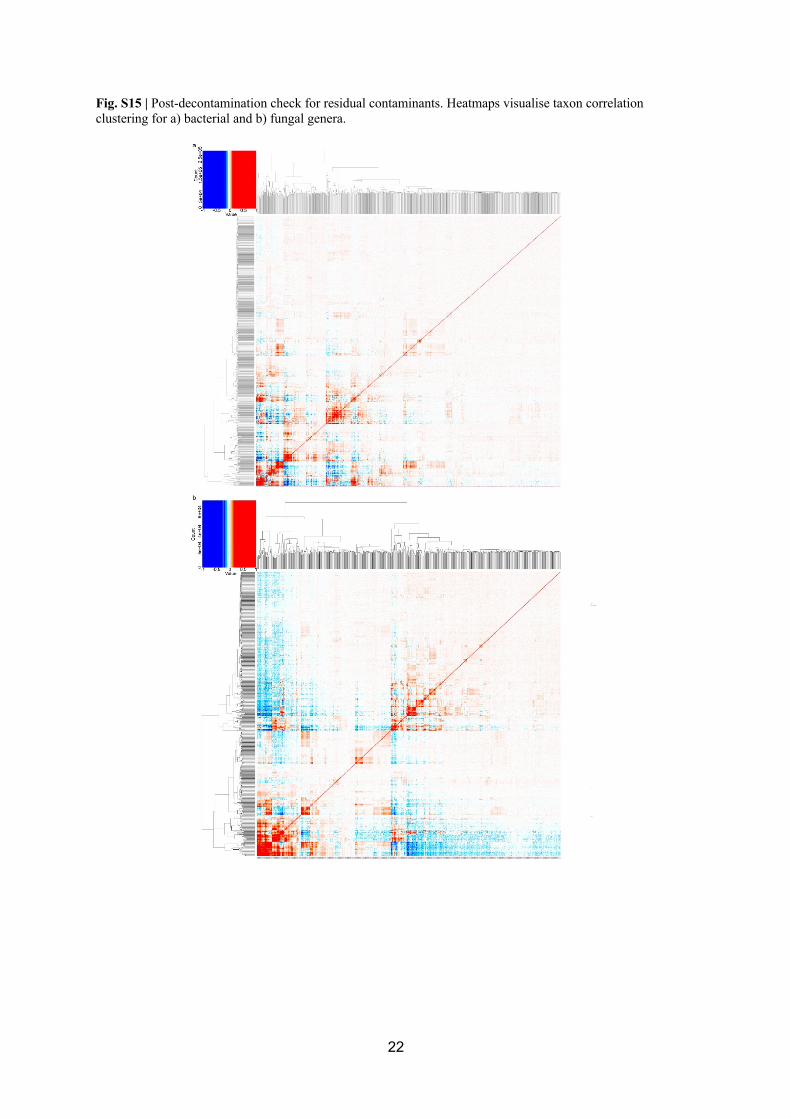
22

Fig. S15 | Post-decontamination check for residual contaminants. Heatmaps visualise taxon correlation

clustering for a) bacterial and b) fungal genera.

23

Fig. S16 | Taxonomic composition of potential residual contaminants. Data shown as a fraction of the filtered

bacterial datasets from different habitats. NG Air = near-ground air, HA Air = high-altitude air.

We further analysed our data to examine the potential for batch effects (cross contamination) because this is of

particular importance when sampling habitats with highly differing biomass such as air and soil. We also

examined our data for potential signals of temporal or spatial auto-correlation.

Several steps were taken to minimise the potential for cross contamination:

1. Soil and air were sampled separately in time (i.e. soil was collected immediately after each air

sampling) and in terms of potential cross-contact (i.e. separate field equipment and processing for soil

and air). All samples (i.e. both soil and air) entered the laboratory in the same state in separate sealed

and surface-sterilised sample tubes as a mixture in nucleic acid preservative solution (i.e. no free soil

particulates were introduced to the laboratory).

2. The processing of all samples was fully randomised for location and habitat type. The randomised

workflow involved some batches where both air and soil samples were processed in the same batch and

others where air samples only were processed, but we conducted two very important steps to check for

potential cross contamination: i) We adopted a workflow where for every batch, each sample tube was

processed individually within a BSL2 flow hood. This means that at any given time during laboratory

work only a single sample tube was opened during processing to reduce the chance of cross-

contamination (the main source of cross-contamination is thought to be micro-fluid splashes between

samples). No multiplexing was employed during pipetting. We believe this was a necessary although

extremely laborious step to avoid cross-contamination. ii) We conducted statistical tests to determine

batch-type did not result in significantly different estimates, i.e. there was no evidence for cross-contamination between soil and air samples. Matching samples (from same location and same sample

types but differing in sequencing batches which had either air samples only or with air and soil

samples) showed significant concordance and low sum of squared errors, thus high goodness of fit

(Bacteria: n = 250, m2 = 0.043333, P = 0.001; Fungi n = 186, m2 = 0.049571, P = 0.001) between their

ordination coordinates (PCoA with Hellinger distance) (Fig. S12). This suggests low influence within

each sequencing batch (the dissimilarities of the communities were preserved regardless of other

samples in the sequencing batches). This was also supported by a Mantel test of the community

distances (Bacteria: n = 250, r = 0.818, P = 0.001; Fungi n = 186, r = 0.915, P = 0.001). These findings

were also supported by our post-decontamination correlation analysis above (Fig. S15), where there it

was clear that cross contamination between air and soil samples had been successfully avoided.

3. In addition, controls were included at all sampling and lab processing stages and these were included in the randomised workflow to check for sampling and laboratory reagent contamination (i.e. controls

were randomly incorporated into each batch). We also employed other stringent measures to avoid

contamination such as full PPE for operators, bleach-sterilization of all laboratory surfaces and

equipment contact surfaces, and UV illumination of workstations when not in use.

4. Our amplicon and metagenome sequencing devices were located in different laboratories and yielded

comparable diversity trends across all samples, which we confirmed statistically using Procrustes

analysis (Bacteria M2 = 0.76, correlation = 0.49, p = 0.001; Fungi M2 = 56, correlation = 0.66, p =

24

0.001). This provided evidence that cross-contamination during sequencing was highly unlikely due to

our randomised workflow.

Matching samples (from same location and same sample types but differ in sequencing batches which had either

air sample only or with air and soil samples) showed significant concordance and low sum of squared errors, thus high goodness of fit (Bacteria: n = 250, m2 = 0.043333, P = 0.001; Fungi n = 186, m2 = 0.049571, P =

0.001) between their ordination coordinates (PCoA with Hellinger distance). This suggests low influence within

each sequencing batch (the dissimilarities of the communities were preserved regardless of other samples in the

sequencing batches). This was also supported by a Mantel test of the community distances (Bacteria: n = 250, r

= 0.818, P = 0.001; Fungi n = 186, r = 0.915, P = 0.001). It was clear from ordinations that sampling date did

not affect location and habitat-specific clustering and so temporal auto-correlation was discounted as a

confounding factor (Bacteria n =449, Fungi n =365) (Fig. S17). We also performed checks using PCNM to

statistically discount the effects of spatial auto-correlation on our findings [37, 38]. Our sampling design was

dominated by very large distances that separated the main locations across the major biomes and continents we

sampled across the globe. Due to the lack of hierarchical structure this design was not intended to account for

smaller spatial scales such as within continents or between locations within the same continent. Because of this

reason, when we applied PCNMs to our dataset, the results indicated that latitude and longitude were the major spatial correlates of the multivariate distribution displayed, as shown in the Results where samples clearly

clustered by geographic location. The simple linear effect of latitude and longitude thus dominated as a simple

expression of the large distance between our sampling locations, and the resulting PCNMs (eigenvectors)

extractable from our distance matrix accounted for such a small amount of variance that we eventually excluded

these vectors after our preliminary check for autocorrelation. We therefore also calculated and reported distance

decay and co-occurrence analysis to add another layer of support that spatial auto-correlation was not a

significant confounding factor on our observations. Our post-decontamination correlation plot for location at

genus level (Fig. S15) also revealed no patterns that support the existence of strong spatial auto-correlation

independent of the differences expected and observed due to different climate and habitat.

We then plotted visualisations of our data to illustrate ASV removed from each location and habitat

type (Fig. S18), and the diversity of filtered ASV in all samples pre- and post-decontamination (Figs S19, S20). We then tested that our robust decontamination protocol did not have a significant impact on the strong

ecological patterns by habitat type and location as highlighted in our manuscript (Fig. 2). We performed

ordinations (tSNE based on Hellinger Distances) for the community separately for raw and filtered data (i.e. pre-

and post-decontamination) (Fig. S21). This was confirmed with strong and significant correlations for both

Procrustes and Mantel tests based on Pearson’s product-moment correlation for congruence for bacteria

(Procrustes m2 = 0.089, correlation = 0.955, P = <0.01 and confirmed by Mantel statistic r = 0.744, P = <0.01);

and fungi (Procrustes m2 = 0.083, correlation = 0.958, P = <0.01 and confirmed by Mantel statistic r =

0.901, P = <0.01).

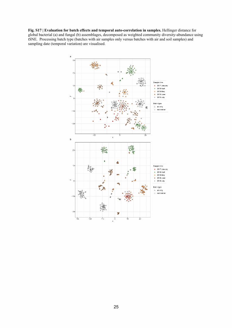
25

Fig. S17 | Evaluation for batch effects and temporal auto-correlation in samples. Hellinger distance for

global bacterial (a) and fungal (b) assemblages, decomposed as weighted community diversity-abundance using

tSNE. Processing batch type (batches with air samples only versus batches with air and soil samples) and

sampling date (temporal variation) are visualised.

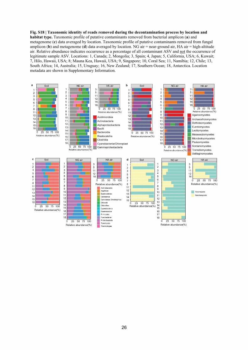
26

Fig. S18 | Taxonomic identity of reads removed during the decontamination process by location and

habitat type. Taxonomic profile of putative contaminants removed from bacterial amplicon (a) and

metagenome (c) data averaged by location. Taxonomic profile of putative contaminants removed from fungal

amplicon (b) and metagenome (d) data averaged by location. NG air = near-ground air, HA air = high-altitude

air. Relative abundance indicates occurrence as a percentage of all contaminant ASV and not the occurrence of legitimate sample ASV. Locations: 1, Canada; 2, Mongolia; 3, Spain; 4, Japan; 5, California, USA; 6, Kuwait;

7, Hilo, Hawaii, USA; 8; Mauna Kea, Hawaii, USA; 9, Singapore; 10, Coral Sea; 11, Namibia; 12, Chile; 13,

South Africa; 14, Australia; 15, Uruguay; 16, New Zealand; 17, Southern Ocean; 18, Antarctica. Location

metadata are shown in Supplementary Information.

27

Fig. S19 | Comparison of bacterial diversity estimation pre- and post-decontamination. Taxonomic

composition for bacteria (for classes ≥0.1% mean relative abundance) for raw data (a) and

post decontamination pipeline (b).

Fig. S20 | Comparison of fungal diversity estimation pre- and post-decontamination. Taxonomic

composition for fungi (for classes ≥0.1% mean relative abundance) for raw data (a) and

post decontamination pipeline (b).

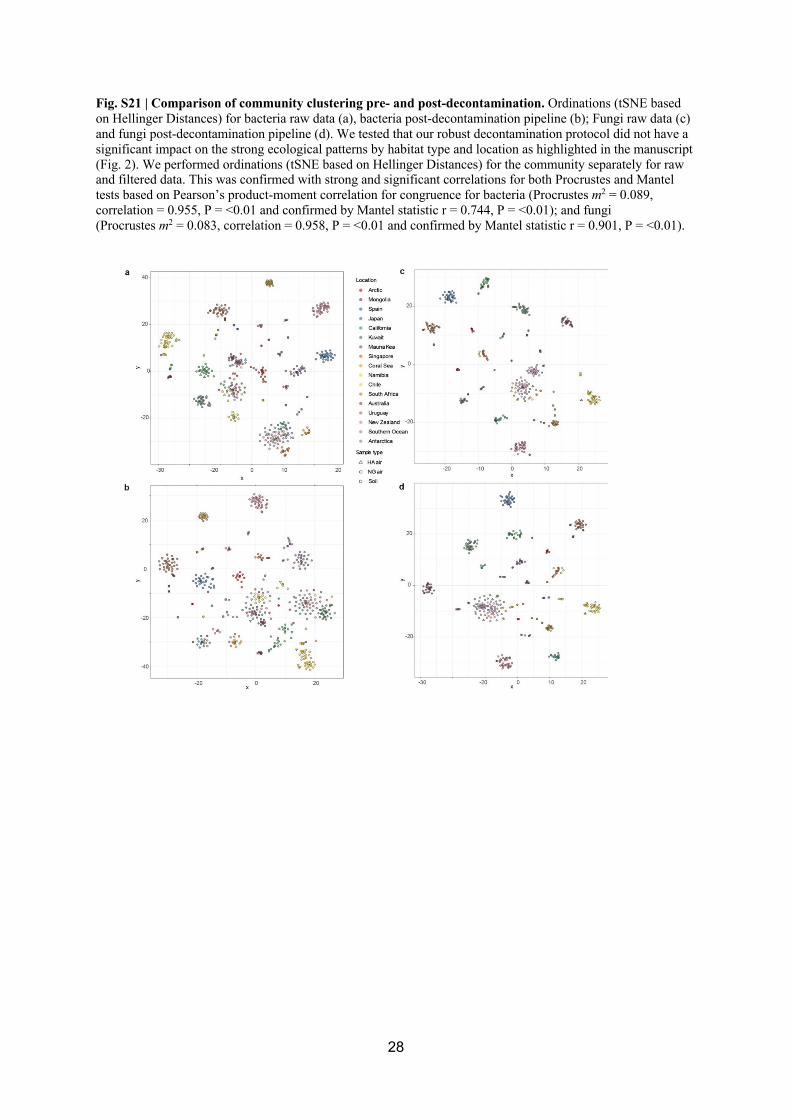
28

Fig. S21 | Comparison of community clustering pre- and post-decontamination. Ordinations (tSNE based

on Hellinger Distances) for bacteria raw data (a), bacteria post-decontamination pipeline (b); Fungi raw data (c)

and fungi post-decontamination pipeline (d). We tested that our robust decontamination protocol did not have a

significant impact on the strong ecological patterns by habitat type and location as highlighted in the manuscript

(Fig. 2). We performed ordinations (tSNE based on Hellinger Distances) for the community separately for raw and filtered data. This was confirmed with strong and significant correlations for both Procrustes and Mantel

tests based on Pearson’s product-moment correlation for congruence for bacteria (Procrustes m2 = 0.089,

correlation = 0.955, P = <0.01 and confirmed by Mantel statistic r = 0.744, P = <0.01); and fungi

(Procrustes m2 = 0.083, correlation = 0.958, P = <0.01 and confirmed by Mantel statistic r = 0.901, P = <0.01).

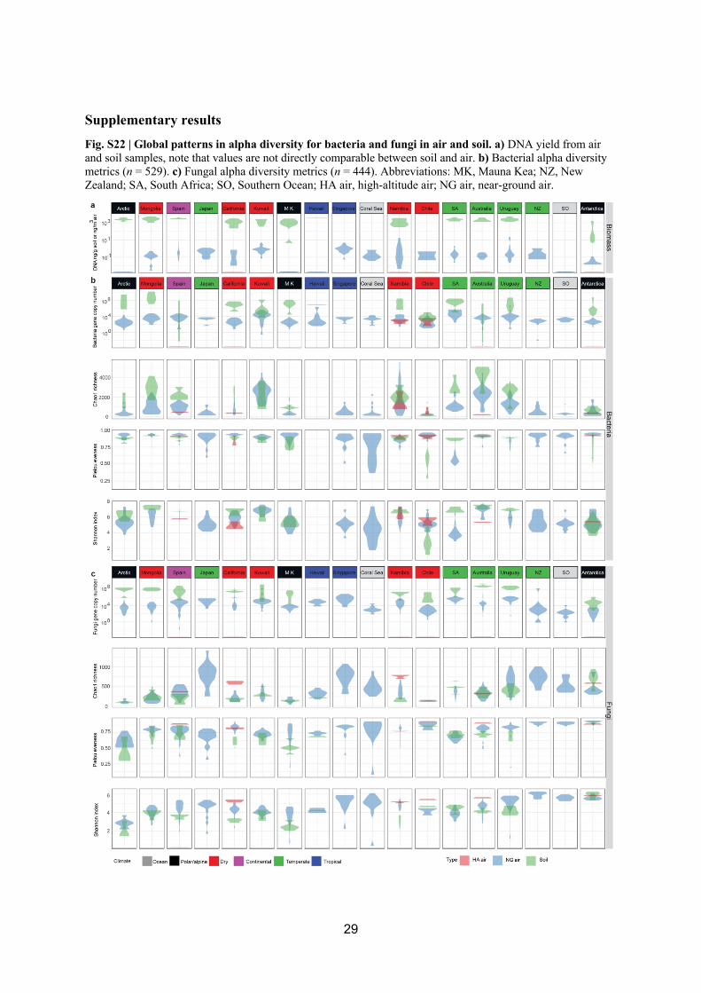
29

Supplementary results

Fig. S22 | Global patterns in alpha diversity for bacteria and fungi in air and soil. a) DNA yield from air

and soil samples, note that values are not directly comparable between soil and air. b) Bacterial alpha diversity

metrics (n = 529). c) Fungal alpha diversity metrics (n = 444). Abbreviations: MK, Mauna Kea; NZ, New

Zealand; SA, South Africa; SO, Southern Ocean; HA air, high-altitude air; NG air, near-ground air.

30

Fig. S23 | Comparison of diversity estimation using shotgun metagenomics and amplicon sequencing of

air and soil. a) Relative abundance of twenty most abundant bacterial phyla estimated from metagenomes (n =

120). b) Relative abundance of twenty most abundant bacterial phyla estimated from amplicon sequencing (n =

529). c) Relative abundance of fungal phyla estimated from metagenomes (n = 120). d) Relative abundance of

fungal phyla estimated from amplicon sequencing (n = 444). Community composition estimation using amplicon sequencing and shotgun metagenomics were positively correlated (Procrustes: Bacteria m2 = 0.76,

correlation = 0.49, P = 0.001; Fungi m2 = 0.56, correlation = 0.66, P = 0.001), and so we focused our fine scale

phylogenetic interrogation on amplicon sequence data because this approach allowed better ecological

representation of the targeted assemblages in terms of sampling depth and taxonomic resolution. Locations: 1,

Canada; 2, Mongolia; 3, Spain; 4, Japan; 5, California, USA; 6, Kuwait; 7, Hilo, Hawaii, USA; 8; Mauna Kea,

Hawaii, USA; 9, Singapore; 10, Coral Sea; 11, Namibia; 12, Chile; 13, South Africa; 14, Australia; 15,

Uruguay; 16, New Zealand; 17, Southern Ocean; 18, Antarctica. HA air, high-altitude air; NG air, near-ground

air; NA, no taxonomy assigned.

Bacteria (amplicon sequencing)

Fungi (amplicon sequencing)

Bacteria (metagenomes)

Fungi (metagenomes)

Ascomycota

Basidiomycota

Blastocladiomycota

Chytridiomycota

Mucoromycota

Zoopagomycota

Mortierellomycota

NA

Relative abundance (%)0 25 50 75 100

1

2

3

5

6

7

8

11

12

13

14

15

18

1

2

3

4

5

6

7

8

9

10

11

12

13

14

15

16

17

18

3

5

11

12

14

18

0 25 50 75 100

Relative abundance (%)

0 25 50 75 100

Relative abundance (%)

0 25 50 75 100Relative abundance (%)

0 25 50 75 100Relative abundance (%)

0 25 50 75 100Relative abundance (%)

Soil NG air HA airSoil NG air HA air

1

2

3

4

5

6

7

8

9

10

11

12

13

14

15

16

17

18

1

2

5

6

7

11

12

13

14

15

3

5

11

12

18

Abditibacteriota

Bdellovibrionota

Desulfobacterota

Myxococcota

Patescibacteria

Sumerlaeota

Acidobacteriota

Actinobacteriota

Aquificae

Armatimonadota

Bacteroidota

Candidatus SaccharibacteriaChlorobi

Chloroflexi

CyanobacteriaDeinococcota

Firmicutes

Fusobacteriota

Gemmatimonadota

Nitrospirota

Planctomycetota

Proteobacteria

Spirochaetes

Synergistetes

Tenericutes

Verrucomicrobiota

Soil NG air HA air

3

5

11

12

14

18

1

2

3

5

6

7

11

12

13

14

15

18

1

2

3

4

5

6

7

9

10

11

12

13

14

15

16

17

18

Soil NG air HA air

1

2

3

5

6

7

8

11

12

13

14

15

18

1

2

3

4

5

6

7

8

9

10

11

12

13

14

15

16

17

18

3

5

11

12

18

Relative abundance (%)0 25 50 75 100

Relative abundance (%)0 25 50 75 100

Relative abundance (%)0 25 50 75 100

Relative abundance (%)0 25 50 75 100

Relative abundance (%)0 25 50 75 100

Relative abundance (%)0 25 50 75 100

a b

c d

31

Table S4 | The effect of habitat and location on structure of bacterial and fungal assemblages. Analysis

was implemented using the R package manyglm for the top 5000 ASV (see Methods). P-values were calculated

using 999 iterations via PIT-trap resampling. Res. Df = Error or Residual Degrees of Freedom, Df.diff =

Difference in degrees of freedom, Dev = Deviance, Pr(>Dev) = P value. Both variables were significant in

structuring bacterial and fungal assemblages.

Bacteria

Res.Df Df.diff Dev Pr(>Dev)

(Intercept) 528

Habitat 526 2 30431 0.001

Location 509 17 368576 0.001

Habitat:Location 492 25 47552 0.19

Fungi

Res.Df Df.diff Dev Pr(>Dev)

(Intercept) 443

Habitat 441 2 23811 0.001

Location 424 17 387268 0.001

Habitat:Location 407 25 47357 0.033

32

Fig. S24 | Dissimilarity of assemblages by habitat type and location. Jaccard Index for global bacterial (a)

and fungal (b) assemblages, decomposed using PCoA. Clustering by habitat type (green, soil; blue, NG air; red,

HA air) was also conserved when analysis was reiterated using only locations where concurrent sampling for all

habitat types occurred to mitigate against potential sample-size effects.

b

a

−1.0−0.5 0.0 0.5 1.0

−0.5

0.0

0.5

1.0

1.5

−0.8−0.6

−0.4−0.2

0.0 0.2

0.4 0.6

0.8

PCoA2 (10%)

PC

oA1

(13%

)

PC

oA3

(7%

)

181

17

2

16

144

15

5

13

7

116

1210 9

318

1

2

1415

5

137

11

6

12

3

18

5

14

11

12 3

−1.0 −0.5 0.0 0.5 1.0

−1.5

−1.0

−0.5

0.0

0.5

1.0

−1.0−0.8

−0.6−0.4

−0.2 0.0

0.2 0.4

0.6

PCoA1 (11%)

PC

oA2

(6%

)

PC

oA3

(5%

)

18

1

17

2

1614

4

15

5

13

7

11

61210

9

3

18

1

2

1415

5

13

7

11

612

3

185

14

1112

3

8

8

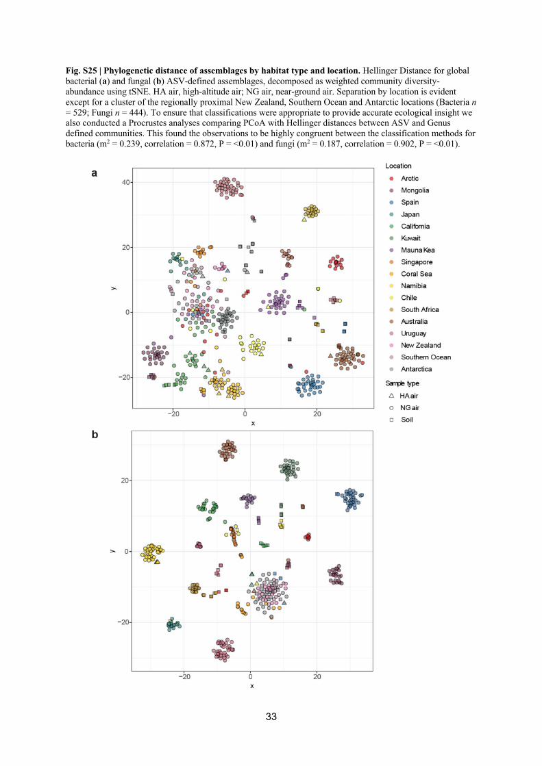
33

Fig. S25 | Phylogenetic distance of assemblages by habitat type and location. Hellinger Distance for global

bacterial (a) and fungal (b) ASV-defined assemblages, decomposed as weighted community diversity-

abundance using tSNE. HA air, high-altitude air; NG air, near-ground air. Separation by location is evident

except for a cluster of the regionally proximal New Zealand, Southern Ocean and Antarctic locations (Bacteria n

= 529; Fungi n = 444). To ensure that classifications were appropriate to provide accurate ecological insight we also conducted a Procrustes analyses comparing PCoA with Hellinger distances between ASV and Genus

defined communities. This found the observations to be highly congruent between the classification methods for

bacteria (m2 = 0.239, correlation = 0.872, P = <0.01) and fungi (m2 = 0.187, correlation = 0.902, P = <0.01).

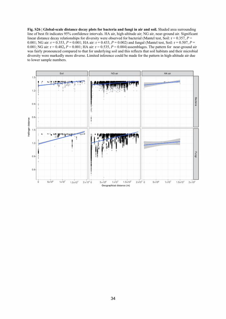
34

Fig. S26 | Global-scale distance decay plots for bacteria and fungi in air and soil. Shaded area surrounding

line of best fit indicates 95% confidence intervals. HA air, high-altitude air; NG air, near-ground air. Significant

linear distance decay relationships for diversity were observed for bacterial (Mantel test, Soil: r = 0.357, P =

0.001; NG air: r = 0.353, P = 0.001; HA air: r = 0.433, P = 0.002) and fungal (Mantel test, Soil: r = 0.507, P =

0.001; NG air: r = 0.482, P = 0.001; HA air: r = 0.535, P = 0.004) assemblages. The pattern for near-ground air was fairly pronounced compared to that for underlying soil and this reflects that soil habitats and their microbial

diversity were markedly more diverse. Limited inference could be made for the pattern in high-altitude air due

to lower sample numbers.

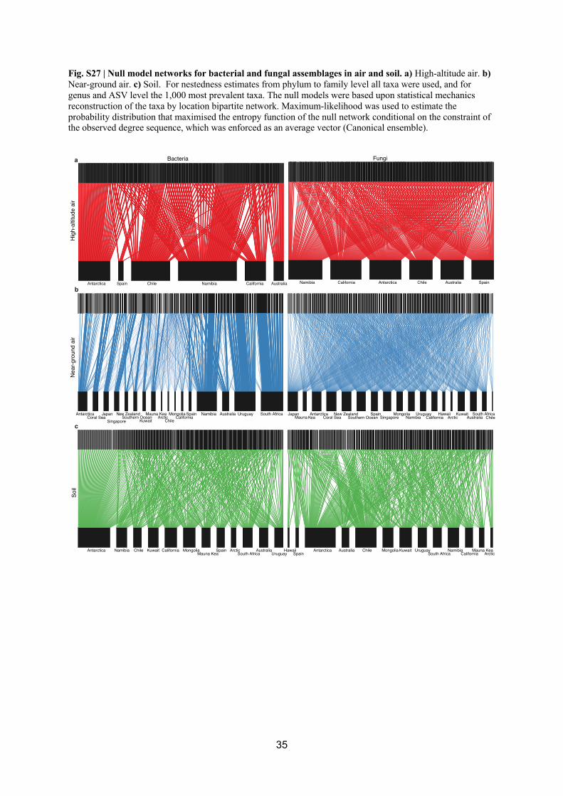
35

Fig. S27 | Null model networks for bacterial and fungal assemblages in air and soil. a) High-altitude air. b)

Near-ground air. c) Soil. For nestedness estimates from phylum to family level all taxa were used, and for

genus and ASV level the 1,000 most prevalent taxa. The null models were based upon statistical mechanics

reconstruction of the taxa by location bipartite network. Maximum-likelihood was used to estimate the

probability distribution that maximised the entropy function of the null network conditional on the constraint of the observed degree sequence, which was enforced as an average vector (Canonical ensemble).

b

a

Antarctica Spain Chile Namibia California Australia Namibia California Antarctica Chile Australia Spain

AntarcticaCoral Sea

Japan

Singapore

New Zealand Southern Ocean

Kuwait

Mauna Kea Arctic

Chile

MongoliaCalifornia

Spain Namibia Australia Uruguay South Africa JapanMauna Kea

AntarcticaCoral Sea

New ZealandSouthern Ocean

SpainSingapore

MongoliaNamibia

UruguayCalifornia

HawaiiArctic

KuwaitAustralia

South AfricaChile

Antarctica Namibia Chile Kuwait California MongoliaMauna Kea

Spain ArcticSouth Africa

AustraliaUruguay

HawaiiSpain

Antarctica Australia Chile Mongolia Kuwait UruguaySouth Africa

NamibiaCalifornia

Mauna Kea Arctic

c

Hig

h-a

ltitude a

irN

ear-

gro

und a

irS

oil

Bacteria Fungi

36

Fig. S28 | Taxonomic composition of bacterial and fungal assemblages in air and underlying soil.

Estimates shown are for ASV-defined assemblages for a) bacteria n = 529) and b) fungi (n = 444). Arrows

indicate locations where aircraft sampling of high-altitude air was undertaken. A taxa filtering criteria of <0.1%

mean relative abundance was used for these plots and so incomplete bars for some samples indicates taxa with

very low abundance rather than unidentified taxa.

a100 200 300 400 500

Sample number

Soil Air

0.00

0.25

0.50

0.75

1.00

Rela

tive a

bundance

TropicalOcean Polar/alpine Dry Continental TemperateClimate

Class

Abditibacteria

Acidimicrobiia

Acidobacteriae

Actinobacteria

Alphaproteobacteria

Anaerolineae

Bacilli

Bacteroidia

Bdellovibrionia

Blastocatellia

Chloroflexia

Clostridia

Cyanobacteriia

Deinococci

Gammaproteobacteria

Gemmatimonadetes

Ktedonobacteria

Longimicrobia

Myxococcia

Oligoflexia

Phycisphaerae

Planctomycetes

Polyangia

Rubrobacteria

Saccharimonadia

Sumerlaeia

Thermoanaerobaculia

Thermoleophilia

Vampirivibrionia

Verrucomicrobiae

Vicinamibacteria

0.00

0.25

0.50

0.75

1.00

Rela

tive a

bundance

100 200 300 400

Sample number

Soil Airb

Class

Agaricomycetes

Archaeorhizomycetes

Arthoniomycetes

Cystobasidiomycetes

Dothideomycetes

Eurotiomycetes

Lecanoromycetes

Leotiomycetes

Malasseziomycetes

Microbotryomycetes

Mortierellomycetes

Pezizomycetes

Rhizophlyctidomycetes

Saccharomycetes

Sordariomycetes

Spizellomycetes

Taphrinomycetes

Tremellomycetes

Ustilaginomycetes

Wallemiomycetes

NA

Chytridiomycetes

Exobasidiomycetes

37

Fig. S29 | Co-occurrence of bacterial and fungal taxa in globally distributed air and soil. The scatterplots

show number of ASVs (Y-axis) shared among ≥ number of samples (X-axis). Generally, fewer ASVs were

shared across larger number of samples. Shared ASVs were determined by simple presence/absence of a given

ASV between two assemblages (Bacteria, n = 529; Fungi n = 444).

Soil NG air HA air

Ba

cte

ria

101

103

105

Nu

mb

er

of

AS

Vs

Fu

ng

i

1 40 1 200 1 9

102

103

104

Shared in > x samples

Nu

mb

er

of

AS

Vs

100 5

-

20

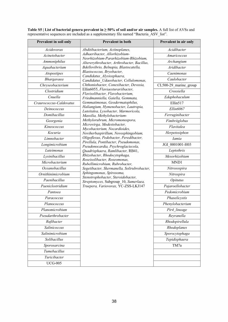
38

Table S5 | List of bacterial genera prevalent in ≥ 50% of soil and/or air samples. A full list of AVSs and

representative sequences are included as a supplementary file named “Bacteria_ASV_list”.

Prevalent in soil only Prevalent in both Prevalent in air only

Acidovorax Abditibacterium, Actinoplanes, Adhaeribacter, Allorhizobium-

Neorhizobium-Pararhizobium-Rhizobium,

Altererythrobacter, Arthrobacter, Bacillus,

Bdellovibrio, Belnapia, Blastocatella,

Blastococcus, Bryobacter,

Candidatus_Alysiosphaera,

Candidatus_Udaeobacter, Cellulomonas,

Chthoniobacter, Conexibacter, Devosia,

Ellin6055, Flaviaesturariibacter,

Flavisolibacter, Flavobacterium,

Friedmanniella, Gaiella, Gemmata,

Gemmatimonas, Geodermatophilus, Haliangium, Hymenobacter, Lautropia,

Luteitalea, Lysobacter, Marmoricola,

Massilia, Methylobacterium-

Methylorubrum, Micromonospora,

Microvirga, Modestobacter,

Mycobacterium, Nocardioides,

Noviherbaspirillum, Novosphingobium,

Oligoflexus, Pedobacter, Peredibacter,

Pirellula, Pontibacter, Pseudomonas,

Pseudonocardia, Psychroglaciecola,

Quadrisphaera, Ramlibacter, RB41, Rhizobacter, Rhodocytophaga,

Roseisolibacter, Roseomonas,

Rubellimicrobium, Rubrobacter,

Segetibacter, Skermanella, Solirubrobacter,

Sphingomonas, Spirosoma,

Stenotrophobacter, Steroidobacter,

Streptomyces, Subgroup_10, Sumerlaea,

Truepera, Variovorax, YC-ZSS-LKJ147

Acidibacter

Acinetobacter Amaricoccus

Ammoniphilus Archangium

Aquabacterium Aridibacter

Atopostipes Caenimonas

Bhargavaea Caulobacter

Chryseobacterium CL500-29_marine_group

Clostridium Crossiella

Cnuella Edaphobaculum

Craurococcus-Caldovatus Ellin517

Deinococcus Ellin6067

Domibacillus Ferruginibacter

Georgenia Fimbriiglobus

Kineococcus Flavitalea

Kocuria Herpetosiphon

Limnobacter Iamia

Longimicrobium JGI_0001001-H03

Luteimonas Leptothrix

Lysinibacillus Mesorhizobium

Microbacterium MND1

Oceanobacillus Nitrosospira

Ornithinimicrobium Nitrospira

Paenibacillus Opitutus

Paeniclostridium Pajaroellobacter

Pantoea Pedomicrobium

Paracoccus Phaselicystis

Planococcus Phenylobacterium

Planomicrobium Pir4_lineage

Pseudarthrobacter Reyranella

Rufibacter Rhodopirellula

Salinicoccus Rhodoplanes

Salinimicrobium Sporocytophaga

Solibacillus Tepidisphaera

Sporosarcina TM7a

Tumebacillus

Turicibacter

UCG-005

39

Table S6 | List of fungal genera prevalent in ≥ 50% of soil and/or air samples. A full list of AVSs and

representative sequences are included as a supplementary file named “Fungi_ASV_list”.

Prevalent in soil only Prevalent in both Prevalent in air only

Acremonium Alternaria Exophiala

Agaricus Aspergillus Knufia

Botrytis Bipolaris Mortierella

Ceriporia Chaetomium Oedocephalum

Cladosporium Coprinellus Powellomyces

Dioszegia Coprinopsis Rhizophlyctis

Ganoderma Curvularia Saitozyma

Gymnopus Didymella Stagonosporopsis

Mycosphaerella Filobasidium Westerdykella

Neoascochyta Fomitopsis

Nigrospora Fusarium

Paradendryphiella Gibberella

Paraphaeosphaeria Naganishia

Phellinus Neocamarosporium

Phlebiopsis Papiliotrema

Psathyrella Penicillium

Resinicium Peniophora

Sarocladium Periconia

Selenophoma Phaeococcomyces

Spegazzinia Phaeosphaeria

Torula Phanerochaete

Toxicocladosporium Phlebia

Trametes Preussia

Tranzscheliella Pseudopithomyces

Tulostoma Vishniacozyma

Udeniomyces

Ustilago

Wallemia

40

Fig. S30 | Source contribution to observed diversity in air. a) Estimated contribution of aquatic, phyllosphere

and soil sources to bacterial diversity. b) Estimated contribution of aquatic, phyllosphere and soil sources to

fungal diversity. Location 3 (Spain) was impacted by a minor intrusion of Sahara Desert atmospheric dust

during sampling. HA air, high-altitude air; NG air, near-ground air. Top row: green shading indicates source

locations sampled in this study, grey boxes indicate data from other studies employed in the meta-analysis. Bottom and right: coloured boxes correspond with climate as shown in Fig. 3. Numbers in each box indicate the

estimate proportion of contribution from a given source (top row) in each sink community (left).

!"#$%#&'(

%)

!*$+"#$%#+&'(

%)

,+-*+&./+&

'(%)

,(*0()%+&'(%)

1+)%2(

"*%+&'(

%)

.-3+

%$&'(

%)

4+5%6%+&'(

%)

17%)/&'(%)

'8+%*

&'(%)

'(-$7&!2"%#+&

'(%)

!-9$"+)%+&'(%)

:"-0-+;&'(

%)

</58/"+$/&

="/973

+$/"

</58/"+$/&

,(-*$+%*

</58/"+$/&

'/>%5

/*$

</58/"+$/&&

'(%)

?+8+*&'/

+

@+#%2%#&A#/+*

B%*/&

@7;))(987/"/

:*C*(3

*

1("+)&'/+& DEDDF DEDGH DEDDD DEDGI DEDGJ DEDDK DEDGH DEDJF DEDDL DEDDI DEDLK DEDDG DEDDD DEDDD DEDDD DEDDD DEDDD DEDDL DEDDG DEILI

'(-$7/"*&A#/+*& DEDLG DEDLG DEDDL DEDLK DEDLJ DEDDF DEDLI DEDJD DEDDD DEDDL DEDLD DEDDH DEDDL DEDDD DEDDD DEDDD DEDDL DEDDD DEDDH DEIMK

!"#$%#& DEDJK DEDGN DEDDG DEDGL DEDLL DEDLL DEDLH DEDLN DEDDJ DEDDL DEDLG DEDDG DEDDL DEDDD DEDDD DEDDD DEDDD DEDDL DEDDG DEIJJ

!*$+"#$%#+& DEDDI DELLL DEDDL DEDGK DEDLN DEDDK DEDLI DEDGK DEDDD DEDDD DEDDM DEDDG DEDDL DEDDL DEDDD DEDDD DEDDL DEDDL DEDDL DENMH

,+-*+&./+& DEDLD DEDGN DEDKL DEDGN DEDLN DEDLD DEDGL DEDGL DEDDF DEDDJ DEDLF DEDDG DEDDL DEDDD DEDDD DEDDD DEDDD DEDDL DEDDJ DENFK

,(*0()%+& DEDDM DEDLG DEDDL DEGGH DEDHI DEDLL DEDFL DEDLG DEDDJ DEDDH DEDLF DEDDM DEDDD DEDDD DEDDD DEDDD DEDDD DEDDD DEDDL DEMDF

1+)%2("*%+& DEDLG DEDGJ DEDLG DEDHJ DELDM DEDLH DEDFD DEDLK DEDDJ DEDDH DEDGG DEDDH DEDDL DEDDD DEDDD DEDDD DEDDD DEDDL DEDDG DEMID

.-3+%$& DEDDL DEDGD DEDDG DEDMD DEDNM DEDFJ DEDFN DEDGD DEDDL DEDDJ DEDLG DEDLF DEDDD DEDDD DEDDD DEDDD DEDDF DEDDJ DEDDH DEMIN

4+5%6%+& DEDDG DEDLD DEDDL DEDGL DEDGK DEDLK DEGJD DEDDI DEDDG DEDLL DEDLN DEDDI DEDDL DEDDL DEDDD DEDDD DEDDD DEDDD DEDDG DEMJI

17%)/& DEDLG DEDLI DEDDL DEDLH DEDLF DEDDM DEDGD DEDJD DEDDD DEDDG DEDLD DEDLD DEDDL DEDDD DEDDD DEDDD DEDDD DEDDL DEDDG DEIMD

'8+%*& DEDJN DEDLK DEDDK DEDFG DEDLF DEDGG DEDDK DEDLL DEDGL DEDLJ DEDKL DEDLN DEDDJ DEDDJ DEDDD DEDDL DEDDD DEDDL DEDDF DEMIF

?+8+*& DEDDI DEDLF DEDDD DEDLI DEDLN DEDDN DEDLI DEDJF DEDDG DEDDM DEDLL DEDDG DEDDD DEDDL DEDDD DEDDD DEDDD DEDDD DEDDJ DEIMD

'(-$7&!2"%#+& DEDDL DEDDJ DEDDD DEDDM DEDDG DEDDJ DEDDL DEDDG DEDDL DEDMN DEDLN DEDDI DEDDG DEDDD DEDDD DEDDD DEDDD DEDDD DEDDL DEIIH

!-9$"+)%+& DEDDH DEDDN DEDDJ DEDHI DEDDN DEDDK DEDDM DEDDF DEDJD DEDGM DEJGL DEDLG DEDDL DEDDG DEDDL DEDDL DEDDL DEDDD DEDDG DEHDM

:"-0-+;& DEDDG DEDDH DEDDL DEDDJ DEDDH DEDGJ DEDDJ DEDDH DEDDG DEDLJ DEDGF DEDLN DEDDF DEDDD DEDDD DEDDD DEDDD DEDDD DEDDK DEIIJ

4/3&O/+)+*>& DEDDH DEDGN DEDDG DEDJJ DEDGF DEDLG DEDGH DEDJN DEDDD DEDDL DEDDK DEDDG DEDDD DEDDD DEDDD DEDDD DEDDD DEDDG DEDDJ DEILI

'%*0+8("/& DEDDJ DEDLK DEDDG DEDLF DEDLJ DEDLD DEDLD DEDGK DEDDD DEDDH DEDDM DEDDJ DEDDL DEDDD DEDDD DEDDD DEDDL DEDDD DEDDF DEINI

!*$+"#$%#+& DEDDD DEDGL DEDJI DEDDD DEDDD DEDDD DEDDG DEDLI DEDDL DEDDD DEDDD DEDDD DEDDD DEDDD DEDDD DEDDD DEDDL DEDDD DEDDD DEKGD

1+)%2("*%+& DEDDN DEDDL DEDDL DEDLD DEDLN DEDDJ DEDLF DEDDN DEDDD DEDDD DEDDI DEDDG DEDDD DEDDD DEDDD DEDDD DEDDD DEDDD DEDDD DEKGK

17%)/& DEDDM DEDDF DEDDL DEDGL DEDDK DEDDF DEDLD DEDGJ DEDDL DEDDF DEDLF DEDDM DEDDL DEDDD DEDDD DEDDD DEDDD DEDDD DEDDN DEIII

4+5%6%+& DEDDJ DEDLM DEDDD DEDGG DEDLH DEDDN DEDMM DEDLK DEDDG DEDDK DEDLD DEDDN DEDDD DEDDD DEDDD DEDDD DEDDL DEDDD DEDDL DEIGG

'8+%*& DEDDD DEDDM DEDDH DEDDL DEDDD DEDDD DEDDD DEDDL DEDDG DEDDL DEDDL DEDDD DEDDD DEDDD DEDDD DEDDD DEDDD DEDDD DEDDL DEKID

!-9$"+)%+& DEDDG DEDDD DEDDD DEDDD DEDDL DEDDL DEDDD DEDDL DEDDG DEDDD DEDDN DEDDD DEDDD DEDDD DEDDD DEDDD DEDDD DEDDD DEDDD DEKIH

P!&+%"

4Q&+%"

!"#$

%#&'(

%)

!*$+

"#$%#

+&'(

%)

,+-

*+&.

/+&'

(%)

,(*

0()%+

&'(%)

1+)%2(

"*%+&

'(%)

.-3+

%$&'(

%)

4+5

%6%+&

'(%)

17%)/

&'(%)

'8+%*

&'(%)

'(-$

7&!2

"%#+&

'(%)

!-9$

"+)%+

&'(%)

:"-0

-+;&

'(%)

<+3+

%%&'(%)

=/5

8/"+

$/&'

(%)

1(*$

%*/*$

+)&'(

%)

>+#%2

%#&&?

#/+*

1"(8

&>7

;))(9

87/"

/

@"+

99&

>7;))

(987

/"/

:*A*

(3*

1("+)&'/+& BCBBD BCDEF BCBBB BCBBF BCBBD BCBBG BCBBF BCBBH BCBBI BCBBJ BCBBH BCBBG BCBBB BCBBB BCBBD BCBBB BCBBB BCBBB BCJJJ

'(-$7/"*&?#/+*& BCBBJ BCKBJ BCBBI BCDBE BCBBH BCBBL BCBBF BCBBH BCBDG BCBDF BCBBK BCBBF BCBBB BCBBD BCBBH BCBBB BCBBB BCBBB BCIDD

!"#$%#& BCBBD BCBBG BCBHG BCBBB BCBBB BCBBI BCBBD BCBBI BCBBB BCBBB BCBBB BCBBB BCBBB BCBBB BCBDE BCBBD BCBBB BCBBD BCLGG

!*$+"#$%#+& BCBBK BCKHI BCBBK BCBEK BCBBG BCBDD BCBBJ BCBBI BCBDD BCBDI BCBBK BCBBG BCBBB BCBBB BCBBI BCBBB BCBBB BCBBB BCIHI

,+-*+&./+& BCBBB BCBDJ BCBJE BCBBB BCBBD BCBBH BCBBH BCBBJ BCBBB BCBBB BCBBD BCBBD BCBBB BCBBB BCBBH BCBBB BCBBB BCBBB BCEEL

,(*0()%+& BCBBB BCBGE BCBBB BCBFG BCBBE BCBBG BCBBD BCBBH BCBBB BCBBB BCBBI BCBBB BCBBB BCBBB BCBBD BCBBB BCBBB BCBBG BCEFK

1+)%2("*%+& BCBBB BCBIB BCBBD BCBBG BCBDI BCBDG BCBBH BCBBE BCBBB BCBBD BCBBG BCBBK BCBBD BCBBB BCBBJ BCBBB BCBBB BCBBI BCLBE

.-3+%$& BCBBB BCBGH BCBBB BCBDK BCBDI BCBFL BCBBD BCBBD BCBBB BCBBI BCBBK BCBBG BCBBB BCBBB BCBBE BCBBB BCBBB BCBBD BCEIE

4+5%6%+& BCBBB BCBIJ BCBBB BCBBD BCBBD BCBDL BCBGG BCBBH BCBBB BCBBG BCBBH BCBBD BCBBB BCBBB BCBBB BCBBB BCBBB BCBBD BCEEE

17%)/& BCBBB BCBBI BCBBB BCBBB BCBBB BCBBH BCBBB BCBBH BCBBB BCBBD BCBBB BCBBI BCBBG BCBBB BCBBB BCBBB BCBBB BCBBB BCLEG

'8+%*& BCBBB BCBHK BCBBI BCBBH BCBBD BCBBI BCBBD BCBBH BCBBH BCBBB BCBBL BCBBH BCBBB BCBBB BCBDB BCBBB BCBBB BCBBL BCLIB

M+8+*& BCBBB BCBHG BCBBB BCBBB BCBBB BCBBB BCBBB BCGJH BCBBB BCBBD BCBBB BCBBF BCBBD BCBBB BCBBB BCBBB BCBBB BCBBB BCGLF

'(-$7&!2"%#+& BCBBB BCBIE BCBBB BCBBD BCBBB BCBBD BCBBH BCBBD BCBBB BCBLE BCBBD BCBBE BCBBB BCBBB BCBBD BCBBB BCBBB BCBBB BCEKB

!-9$"+)%+& BCBBB BCBHG BCBBB BCBHK BCBBG BCBBF BCBBD BCBBG BCBBB BCBBI BCBEH BCBBB BCBBB BCBBB BCBBE BCBBB BCBBB BCBBB BCEGD

:"-0-+;& BCBBB BCHEB BCBBB BCBBB BCBBB BCBBD BCBBB BCBBE BCBBB BCBBB BCBBD BCBDE BCBBB BCBBB BCBBI BCBBB BCBBB BCBBB BCFEE

4/3&N/+)+*O& BCBBK BCKID BCBBD BCBFJ BCBBG BCBBE BCBBE BCBBG BCBDB BCBBE BCBBK BCBBK BCBBB BCBBB BCBBI BCBBB BCBBB BCBBB BCIGB

<+3+%%& BCBBB BCBBK BCBBD BCBBD BCBBB BCBBB BCBBB BCBBE BCBBB BCBBB BCBBB BCBBB BCBBD BCBBB BCBBB BCBBB BCBBB BCBBB BCLEG

'%*0+8("/& BCBBB BCBDB BCBBD BCBBB BCBBB BCBBH BCBBD BCBBJ BCBBB BCBBD BCBBB BCBBD BCBBD BCBBB BCBBB BCBBB BCBBB BCBBB BCLJF

!*$+"#$%#+& BCBBD BCILD BCBBG BCDIE BCBBF BCBBI BCBBH BCBBH BCBDI BCBBE BCBBG BCBBG BCBBB BCBBH BCBBH BCBBB BCBBB BCBBD BCGDL

1+)%2("*%+& BCBBD BCHBJ BCBBD BCBDD BCBBF BCBBJ BCBBH BCBBH BCBBH BCBBH BCBBH BCBBI BCBBB BCBBB BCBBH BCBBB BCBBB BCBBH BCJGE

17%)/& BCBBF BCHFE BCBBB BCBHB BCBBB BCBBF BCBBJ BCBBB BCBBH BCBBG BCBBL BCBBK BCBBI BCBBB BCBBI BCBBB BCBBB BCBBB BCFFE

4+5%6%+& BCBBH BCDDE BCBBK BCBBL BCBBD BCBBL BCBDG BCBBD BCBBD BCBBJ BCBBH BCBBD BCBBB BCBBB BCBBB BCBBB BCBBB BCBBD BCEHJ

'8+%*& BCBBK BCHHG BCBBH BCBGF BCBBD BCBBH BCBBD BCBBD BCBBE BCBDB BCBBG BCBBF BCBBB BCBBB BCBBD BCBBB BCBBB BCBBD BCFEE

!-9$"+)%+& BCBBL BCHEL BCBBB BCBGD BCBBJ BCBBG BCBBK BCBBD BCBBJ BCBBL BCBBE BCBBI BCBBB BCBBB BCBDB BCBBB BCBBB BCBBB BCFBG

<!

&+%"

4@

&+%"

a

b

0 0.02 >0.1Sample contribution

a b c

d

e

f g

j

k lhTem

pera

te s

oil

iC

ontinenta

l soil

41

Fig. S31 | Functional metagenomics profiling of targeted stress-response and metabolic genes by habitat

type. Abundance values for selected genes of the included stress-response and metabolic pathways are

expressed on the heatmap as copies per million reads. The illustrated values represent all samples (total n = 120)

within each air and soil sample group. HA air, high-altitude air; NG air, near-ground air. Gene abundance data

were expressed in terms of copies per million reads from HUMAnN, which takes into account library size differences between samples. For functional gene analysis, differentially more abundant genes in air versus soil

were inversely correlated with biomass and taxonomic richness, they affiliated with taxa observed as enriched in

air, and all values were averaged by location. We therefore interpreted the elevated abundance of genes in air as

reflective of assemblage composition rather than an artefact of sampling effort.

42

Supplementary references

1. Pointing SBSB, Belnap J. Disturbance to desert soil ecosystems contributes to dust-mediated impacts at

regional scales. Biodivers Conserv 2014; 23: 1659–1667.

2. Archer SDJ, Lee KC, Caruso T, King-Miaow K, Harvey M, Huang D, et al. Air mass source determines

airborne microbial diversity at the ocean–atmosphere interface of the Great Barrier Reef marine

ecosystem. ISME J 2020; 14: 871–876.

3. Archer SDJ, Lee KC, Caruso T, Maki T, Lee CK, Cary SC, et al. Airborne microbial transport limitation

to isolated Antarctic soil habitats. Nat Microbiol 2019; 4: 925–932.

4. Peel MC, Finlayson BL. Updated world map of the Köppen-Geiger climate classification. Hydrol Earth

Syst Sci 2007; 11: 1633–1644.

5. University of East Anglia Climatic Research Unit; Harris, I.C.; Jones, P.D.; Osborn T. No Title. CRU

TS4.04: Climatic Research Unit (CRU) Time-Series (TS) version 4.04 of high-resolution gridded data of month-by-month variation in climate (Jan. 1901- Dec. 2019). .

6. Beck HE, Zimmermann NE, McVicar TR, Vergopolan N, Berg A, Wood EF. Present and future

köppen-geiger climate classification maps at 1-km resolution. Sci Data 2018; 5: 1–12.

7. Fischer G. World Food and Agriculture to 2030/50: How do climate change and bioenergy alter the

long-term outlook for food, agriculture and resource availability? Expert Meet. How to Feed World

2050. 2009. pp 1–49.

8. Stein AF, Draxler RR, Rolph GD, Stunder BJB, Cohen MD, Ngan F. NOAA’s HYSPLIT Atmospheric

Transport and Dispersion Modeling System. Bull Am Meteorol Soc 2015; 96: 2059–2077.

9. Burrows SM, Butler T, Jöckel P, Tost H, Kerkweg A, Pöschl U, et al. Bacteria in the global atmosphere

- Part 2: Modeling of emissions and transport between different ecosystems. Atmos Chem Phys 2009; 9:

9281–9297. 10. Dybwad M, Skogan G, Blatny JM. Comparative testing and evaluation of nine different air samplers:

End-to-end sampling efficiencies as specific performance measurements for bioaerosol applications.

Aerosol Sci Technol 2014; 48: 282–295.

11. Garratt JR. Review: the atmospheric boundary layer. Earth Sci Rev 1994; 37: 89–134.

12. Luhung I, Uchida A, Lim SBY, Gaultier NE, Kee C, Lau KJX, et al. Experimental parameters de fi ning

ultra-low biomass bioaerosol analysis. npj Biofilms Microbiomes 2021; 7: 37.

13. Gotelli NJ. Null model analysis of species co-occurrence patterns. Ecology 2000; 81: 2606–2621.

14. Gotelli NJ, Ulrich W. Statistical challenges in null model analysis. Oikos 2012; 121: 171–180.

15. Dormann CF, Strauss R. A method for detecting modules in quantitative bipartite networks. Methods

Ecol Evol 2014; 5: 90–98.

16. Dormann CF, Frund J, Bluthgen N, Gruber B. Indices, Graphs and Null Models: Analyzing Bipartite

Ecological Networks. Open Ecol J 2009; 2: 7–24. 17. Payrató-Borràs C, Hernández L, Moreno Y. Breaking the Spell of Nestedness: The Entropic Origin of

Nestedness in Mutualistic Systems. Phys Rev X 2019; 9: 31024.

18. Artzy-Randrup Y, Stone L. Generating uniformly distributed random networks. Phys Rev E 2005; 72:

56708.

19. Roberts ES, Coolen ACC. Unbiased degree-preserving randomization of directed binary networks. Phys

Rev E 2012; 85: 46103.

20. Squartini T, Garlaschelli D. Maximum-entropy networks: Pattern detection, network reconstruction and

graph combinatorics. 2017. Springer.

21. Saracco F, Di Clemente R, Gabrielli A, Squartini T. Randomizing bipartite networks: the case of the

World Trade Web. Sci Rep 2015; 5: 10595.

22. Garlaschelli D, Loffredo MI. Maximum likelihood: Extracting unbiased information from complex networks. Phys Rev E 2008; 78: 15101.

23. Squartini T, Mastrandrea R, Garlaschelli D. Unbiased sampling of network ensembles. New J Phys

2015; 17: 23052.

24. Ulrich W, Almeida-Neto M, Gotelli NJ. A consumer’s guide to nestedness analysis. Oikos 2009; 118:

3–17.

25. Etienne RS. A neutral sampling formula for multiple samples and an ‘exact’ test of neutrality. Ecol Lett

2007; 10: 608–618.

26. Kembel SW. Disentangling niche and neutral influences on community assembly : assessing the

performance of community phylogenetic structure tests. Ecol Lett 2009; 12: 949–960.

27. Caruso T, Chan Y, Lacap DC, Lau MCY, McKay CP, Pointing SB. Stochastic and deterministic

processes interact in the assembly of desert microbial communities on a global scale. ISME J 2011; 5:

1406–1413. 28. Caruso T, Hempel S, Powell JR, Barto EK, Rillig MC. Compositional divergence and convergence in

arbuscular mycorrhizal fungal communities. Ecology 2012; 93: 1115–1124.

43

29. Maaß S, Migliorini M, Rillig MC, Caruso T. Disturbance, neutral theory, and patterns of beta diversity

in soil communities. Ecol Evol 2014; 4: 4766–4774.

30. Salter SJ, Cox MJ, Turek EM, Calus ST, Cookson WO, Moffatt MF, et al. Reagent and laboratory

contamination can critically impact sequence-based microbiome analyses. BMC Biol 2014; 12: 87.

31. Eisenhofer R, Minich JJ, Marotz C, Cooper A, Knight R, Weyrich LS. Contamination in Low Microbial Biomass Microbiome Studies: Issues and Recommendations. Trends Microbiol 2019; 27: 105–117.

32. Nguyen NH, Smith D, Peay K, Kennedy P. Parsing ecological signal from noise in next generation

amplicon sequencing. New Phytol 2015; 205: 1389–1393.

33. Karstens L, Asquith M, Davin S, Fair D, Gregory WT, Wolfe AJ, et al. Controlling for contanmnninants

in low biomass 16S rRNA gene sequencing experiemnts. mSystems 2019; 4: e00290-19.

34. Sheik CS, Reese BK, Twing KI, Sylvan JB, Grim SL, Schrenk MO, et al. Identification and removal of

contaminant sequences from ribosomal gene databases: Lessons from the Census of Deep Life. Front

Microbiol 2018; 9: 1–14.

35. Els N, Larose C, Baumann-Stanzer K, Tignat-Perrier R, Keuschnig C, Vogel TM, et al. Microbial

composition in seasonal time series of free tropospheric air and precipitation reveals community

separation. Aerobiologia (Bologna) 2019; 35: 671–701.

36. Kiledal EA, Keffer JL, Maresca JA. Bacterial Communities in Concrete Reflect Its Composite Nature and Change with Weathering. mSystems 2021; 6: e-01153-20.

37. Dray S, Legendre P, Peres-Neto PR. Spatial modelling: a comprehensive framework for principal

coordinate analysis of neighbour matrices (PCNM). Ecol Modell 2006; 196: 483–493.

38. Rangel TF, Diniz-Filho JAF, Bini LM. SAM: a comprehensive application for Spatial Analysis in

Macroecology. Ecography (Cop) 2010; 33: 46–50.