District Subdivision and the Location of SmallholderForest Conversion in Sumatra

Marc N. Conte and Philip ShawDepartment of Economics

Fordham University∗

March 9, 2017

∗Email: mconte7@fordham.edu (corresponding author), pshaw5@fordham.edu; Mailing Address: Ford-ham University Department of Economics Dealy Hall 441 E Fordham Rd Bronx, New York 10458

Abstract

A unique GIS data set from Indonesia that distinguishes smallholder and planta-tion operations is used to test the impact of district subdivision, which enhances localcontrol of natural-resource revenues, on the location of smallholder forest conversion.Nonparametric analyses find that in subdivided districts, smallholders convert forestson steeper land that is further from the nearest road and deeper into the forest. Small-holders are also less responsive to forest protection in subdivided districts. Districtsubdivision imposes a welfare loss of $1, 734 to $5, 256 per hectare (in 2010 USD) fromthe increased carbon emissions associated with smallholder conversion deeper in theforest. JEL: C14, Q15

Key Words: Decentralization, Forest conversion, Nonparametrics

1 Introduction

Tropical forests are particular natural resources with several related ecosystem services

that have become an international concern due to the emission of greenhouse gases stemming

from conversion of these forests to production systems. Reducing greenhouse gas emissions

from tropical forest conversion is viewed as a critical component of plans to mitigate the

effects of anthropogenic climate change, as forest clearing accounts for an estimated 12-15%

of global greenhouse gas emissions (van der Werf et al., 2009). Efficient management of

these resources includes the location of forest conservation and conversion, due to landscape

heterogeneity.

The management of tropical forests in Indonesia is of global concern as this nation is in

the top three in terms of extant stands of tropical forest and has forests that are home

to countless endemic species. Rapid conversion to production systems has made Indonesia

the top-ranked nation for deforestation (Margono et al., 2014), and consequently among the

highest green-house gas emitters.

A key change in Indonesia with implications for forest conversion was the decentralization

that occurred in the wake of Suharto’s resignation of the presidency in 1998 due to the Asian

financial crisis of 1997. To keep the nation intact, the post-Suharto regime decentralized the

management of natural resources in Indonesia. As a result, district agencies were respon-

sible for managing the resources in their territories and were more responsible for revenue

generation than under the centralized power structure of Suharto’s regime.

Given the financial pressures associated with the depreciation of the rupiah following

the Asian financial crisis and claims of inequitable distribution of royalties from Jakarta,

resource-rich regions were vocal in their demand for more of the revenue raised from natural

1

resources (forests, gas, oil) to stay under local control (Hofman and Kaiser, 2004). Following

Suharto’s resignation in 1998, laws were enacted to transition control of these resources to

the district agencies (Potter and Badcock, 2001), and as a result many districts subdivided,

ostensibly to secure as much control of their resources as possible (Burgess et al., 2012).

Analysis of the determinants of district subdivision found that large, ethnically-clustered

districts with high staffing levels and substantial natural resource stocks were more likely to

rezone between 1998 and 2000 (Fitrani et al., 2005).

Previous research has considered the impact of this wave of district subdivision in Indonesia

on aggregate deforestation. Regardless of the mechanism studied, this work has shown that

subdivision leads to more forest conversion and plantation activity. Burgess et al. (2012) finds

that the increased number of political jurisdictions increased deforestation due to logging

and reduced timber prices across Indonesia, which is consistent with districts engaged in

Cournot competition as firms choose where to log. Suwarno et al. (2015) uses surveys of

government officials and stakeholders to evaluate forest governance quality. The authors find

that deforestation has increased in Central Kalimantan as a result of district subdivision,

because the quality of forest governance declined with district subdivision.

In this paper, we explore the impact of district subdivision in the wake of Suharto’s res-

ignation on the location of smallholder forest conversion in Sumatra. Previous studies have

shown that while decentralization of natural resource management can offer empowerment

and democratization of local communities as well as poverty reduction through more equi-

table access to resources, decentralization can in fact lead to further marginalization of poor

and disadvantaged groups, with resource control accruing to the most powerful stakeholders

(e.g., Berkes, 2010; Colfer and Capistrano, 2002; Larson and Soto, 2008; Ribot et al., 2006).

In Indonesia, district agencies grant concessions to plantation operators that convey secure

property rights to the plantations and collect royalties from plantation operations. Small-

holder production systems are not taxed and are not formally recognized by these agencies,

2

meaning that smallholder tenure is insecure in the presence of plantations. The increased

level of plantation activity in subdivided districts is expected to impact smallholder forest

conversion given previous research documenting tensions between these two forces of forest

conversion (see e.g., Afrizal, 2007; Casson, 2000; Colchester et al., 2006; McCarthy, 2004;

Potter, 1999; Suyanto, 2007; Suyanto et al., 2004).

Using a unique GIS dataset of 2008 land use and land cover that distinguishes between

smallholder and plantation production at a fine spatial scale, we explore the proximate

determinants of smallholder forest conversion in subdivided and non-subdivided districts

between 2000 and 2008. We estimate these determinants on a randomly-drawn set of pixels

as well as on a set of pixels that lie within five kilometers of a district with the other

subdivision status to ensure that the observed differences in the likelihood of smallholder

conversion are due to district subdivision.

Our analysis shows that the proximate causes of smallholder conversion vary across dis-

tricts with different subdivision status. Specifically, we find that smallholders in non-

subdivided districts have a revealed preference for low-slope parcels that are near the edge of

the forest and close to the nearest road. In subdivided districts, the location of smallholder

production is not affected by slope or distance to the nearest road, and there is only a small

reduction in conversion probability associated with increasing distance from the forest edge.

These results suggest that the location of smallholder forest conversion, and therefore its

private returns and external costs, is affected by district subdivision. We find that district

subdivision leads to additional costs to society, stemming from increased CO2 emissions due

to the location of smallholder conversion further into the forest in subdivided districts, of

$1,734 to $5,256 per hectare.

Our findings suggest that policy action to encourage efficient forest management in Suma-

tra must address both the location and amount of forest conversion. Doing so requires a

3

comprehensive approach that acknowledges both smallholders and plantations as forces of

forest conversion, unlike the 2011 trial moratorium on plantation concessions in extant forests

in Sumatra. We show that district subdivision, with a focus on generation of natural-resource

royalties, leads to increased external costs of smallholder forest conversion, indicating that

decentralization may have increased the challenges to effective forest management in Indone-

sia.

2 Study Area Background

President Suharto’s New Order regime, which was in power from 1966-1998, was strong and

highly-centralized. Under this system, royalties generated from the management of natural

resources (e.g., agricultural plantations, petroleum extraction, and timber harvest) were

sent to the seat of the federal government in Jakarta for redistribution to local government

agencies. The centralized distribution of locally-generated tax revenues was not popular

among officials from particularly resource-rich regions of the nation who felt that the access

to these resources had too frequently been granted to private-sector corporations with ties

to decision-makers in Jakarta (Potter and Badcock, 2001).1

Suharto was forced to resign his Presidency due to fallout from the 1997 financial crisis in

Asia, which sent the rupiah into a major depreciation that lasted through 1998. During this

time, there were calls by resource-rich provinces for independence, and Indonesia underwent

an extensive, and immediate, wave of decentralization under the new regime to appease calls

for more regional autonomy, while maintaining the extent of the nation (Potter and Badcock,

2001).

Several pieces of legislation facilitated the transfer of authority to provincial and district

governments, allowing resource-rich regions to retain a greater share of the revenues gener-

ated within their jurisdictions (Potter and Badcock, 2001). Law 22 on Regional Governance

4

and Law 25 on Fiscal Balancing were issued in May of 1999 and together provided a foun-

dation for the decentralization of administrative and regulatory authority primarily to the

district level. Law 22 defined the sectors that would move to district control from federal

management, including agriculture, forests and fisheries, mining, environment, and land use.

Law 25 simultaneously established that more income from natural-resource sales would be

directed to districts and established that the districts would be expected to take more active

roles in seeking their own sources of revenue. Together, these laws aimed to increase the

generation of district royalties through increased natural-resource use, including increased

issuance of concessions to plantation operators.

In the wake of the national legislation supporting local oversight of natural resources,

many districts chose to subdivide following the end of Suharto’s reign. By altering district

borders, officials in district agencies would give themselves greater control over the natural

resources found within their districts. Between 1998 and 2008, the total number of districts

in Indonesia increased from 292 to 483, as local governments attempted to exert maximum

control over the natural resource royalties originating in their district (Burgess et al., 2012).

The Provinces of Riau, Jambi, and West Sumatra on the island of Sumatra have expe-

rienced a significant amount of forest conversion since the mid-1990s, chiefly as a result of

the rising price of palm oil that has made oil palm plantations quite profitable in the region

(figure 1). These provinces cover an area of approximately 17 million hectares. From 1990 to

2008, 7 million hectares of forest, or 58% of the total forested area in 1990, in these provinces

was converted to production systems (figure 2). The two broad categories of production sys-

tems responsible for forest conversion within these three provinces of Sumatra are industrial

plantation systems and smallholder operations. While plantations are responsible for the

majority of forest conversion in this area, smallholder production has been responsible for

approximately 30% of forest conversion since 1990.

5

Tensions exist between these two drivers of forest conversion because smallholders only

have informal rights to forested parcels on the landscape. Smallholder production systems

are frequently interrupted by corporations developing plantations that have been granted

forest concessions by government agencies (Suyanto et al., 2004). Government agencies

have incentives to provide plantation concessions, as revenues from these systems generate

royalties that are used to support government activities, whereas smallholders are typically

not taxed (Potter and Badcock, 2001).

Concessions are granted to corporations without acknowledgement of the informal cultiva-

tion rights that have been used to allocate areas for harvest within rural communities. This

can result in two outcomes: incorporation of the communal producers into the corporate

production system, or the forced, uncompensated relocation of smallholder production to

lands not covered by the corporate lease rights.2 Given that these agreements are perceived

to be unfair, local smallholders rarely participate in these arrangements and most planta-

tions, including those in the nucleus system, rely on labor imported from other islands (e.g.,

Java) (McCarthy, 2007).

Wages offered to local smallholders in exchange for plantation labor are typically viewed

as unjust by smallholders and promised payments are occasionally not delivered, while land-

grabbing by plantations is not an infrequent occurrence (Afrizal, 2007; Colchester et al.,

2006). Suyanto (2007) provides examples of smallholder production being cleared by planta-

tions through the use of fire, even when the land was not included in the formal concession

to the plantation operator. Disputes between smallholders and plantations in the nuclear

estate scheme often culminate in violence (Casson, 2000).

The next section presents a model of smallholder forest conversion, in which the location

of smallholder conversion is affected by district subdivision. The model predictions will be

tested using data on the location of smallholder forest conversion in Sumatra.

6

3 Model of smallholder location choice

Assume that there is a single production system and that smallholders attempt to max-

imize the expected returns to production by choosing a location in the forest at which

to establish cultivation systems.3 The choice of conversion location is reduced to a one-

dimensional problem to clearly motivate the empirical analysis, which considers a vector of

parcel characteristics related to forest conversion. Let d measure the distance from the forest

edge at which conversion occurs. The net returns to production conditional on maintaining

control of the production system, π(d), are given by

π(d) = P × Y (d)− C(d)

where P represents the market price for the good produced, Y (d) represents the yield of

the product, and C(d) represents the cost of conversion and production, which is expected

to increase at an increasing rate with distance from the forest edge (C ′(d), C ′′(d) ≥ 0,

C ′(0) = 0).4

Plantation activity is expected to be higher in subdivided districts than in non-subdivided

districts. This assumption follows from the findings that deforestation increased following

district subdivision in previous studies (e.g., Burgess et al., 2012; Suwarno et al., 2015).

Let S represent a district’s subdivision status, with S = 1 indicating a district that has

been subdivided, and S = 0 indicating a district that has not. Let L(d, S) represent the

probability that a forest patch is converted by a plantation. Assume that the probability

of plantation interruption is decreasing in distance from the forest edge for the same reason

that smallholder production costs increase with distance from the forest edge. Further,

assume that L(0, S = 1) > L(0, S = 0) and that L′(d, 0) ≤ L′(d, 1) ≤ 0 ∀ d, meaning

that subdivision increases plantation activity at all distances from the forest edge. Such an

outcome might describe a situation in which subdivided districts attract plantations in the

7

hopes of generating royalties from concessions and competition drives plantations further

into the forest in these districts.

To incorporate the probability of a smallholder losing control of the land to a plantation,

consider the following progression of events. At the start of the period, the smallholder makes

a choice about the distance from the forest edge at which to convert the forest to production.

Before the end of the period, smallholder production is either interrupted by plantation

activity or allowed to continue. At the end of the period, the smallholder receives the returns

from production if her operation is not interrupted by plantations. If smallholder production

is interrupted by plantation operations, then the smallholder receives compensation, if any,

from the plantation manager at the end of the period. Then, the smallholder’s problem is

given by

maxd

(1− L(d, S))π(d) + L(d, S)W (d) (1)

where W (d) represents the compensation that the smallholder receives from the plantation

operator for taking her land, which again decreases with increasing forest-edge distance (i.e.,

W ′(d) < 0, W ′′(d) > 0).

Recall that L(0, S = 1) > L(0, S = 0) by assumption. Given this, it follows that

(1− L(0, 0))π(0) + L(0, 0)W (0) > (1− L(0, 1))π(0) + L(0, 1)W (0)

meaning that the expected value of smallholder conversion at the forest edge in non-subdivided

districts is greater than that in subdivided districts. This result generates an empirically-

testable prediction related to the probability of smallholder conversion at the forest edge:

Prediction 1: The probability of smallholder conversion at the forest edge will begreater in non-subdivided districts than in subdivided districts

8

The optimal location of smallholder forest conversion, d∗, satisfies

(1− L(d∗, S))π′(d∗) = L′(d∗, S)[π(d∗)−W (d∗)]− L(d∗, S)W ′(d∗) (2)

The LHS of equation 2 represents the change in the expected net returns of smallholder

production if she is able to maintain control of her production system with increasing forest-

edge distance, π′(d∗), which is the marginal cost of moving production further into the forest.

The RHS of equation 2 represents the change in the expected net returns of smallholder

production conditional on losing control of the land to the plantation operator, which is the

marginal benefit of moving production deeper into the forest. Then, the optimal distance

into the forest at which the smallholder should locate conversion satisfies:

π′(d∗) =L′(d∗, S)[π(d∗)−W (d∗)]− L(d∗, S)W ′(d∗)

(1− L(d∗, S))(3)

Comparative statics can be used to relate the optimal location of forest conversion in

subdivided and non-subdivided districts. Note that ∂π′(d∗)∂L(d∗,S)

= −W ′(d∗)(1−L((d∗,S))2 ≥ 0. Also note

that ∂π′(d∗)∂L′(d∗,S)

= π(d∗)−W (d∗)1−L(d∗,S) ≥ 0. This term is strictly positive with insecure smallholder

tenure (meaning that π(d) > W (d)).

Given these results, it is left to compare L(d∗, 0) and L(d∗, 1). Because L(0, 0) < L(0, 1)

and L′(d, 0) ≤ L′(d, 1) ∀ d, the above comparative statics indicate that d∗1 > d∗0, where d∗0

and d∗1 are the optimal locations of conversion in non-subdivided and subdivided districts,

respectively. This result leads to the following prediction:

Prediction 2: At some positive distance into the forest, the probability of small-holder conversion in subdivided districts will be greater than that in non-subdivideddistricts.

9

The above results suggest how district subdivision can have efficiency effects regarding

the location of smallholder conversion. In an effort to escape plantation taking, smallholders

may convert forest that is undesirable to plantations, lowering the returns to smallholder

production. The model presents this issue in the context of edge distance, though its pre-

dictions can easily be extended to other parcel characteristics (e.g., distance to the nearest

road, slope, etc.). Of additional concern from a welfare perspective is that the external

costs of forest conversion, including edge effects that impact endemic species and the loss of

ecosystem-service production, which are not captured in the smallholder’s problem, increase

with conversion of more remote forest patches. In our welfare analysis, we will focus on the

edge effect regarding carbon storage and sequestration, which was recently shown to be more

significant and persistent than previously thought (Chaplin-Kramer et al., 2015b).

Based on existing results from the literature, this model assumes that district subdivision

increases plantation activity due to an underlying need to generate revenues from the man-

agement of local natural resources. Therefore, district subdivision is predicted to affect the

location of smallholder conversion, which may lead to welfare losses due to the increased

external costs of forest conversion away from the forest edge. The predicted effects will be

tested using detailed land-use and land cover data from central Sumatra.

4 Data

This analysis explores how district subdivision affects whether or not forested land is

converted to smallholder production systems, given the presence of plantation operations on

the landscape. Satellite data provides the best opportunity to account for both legal and

illegal forest conversion, which is necessary to obtain accurate estimates of conversion rates

and the determinants of conversion (Burgess et al., 2012).

10

4.1 Data sets

The key data for this analysis are maps of land-use and land cover (LULC) from 2000

and 2008. The 2000 LULC map is based on Landsat imagery and identifies pixels as either

forest or non-forest. The map of LULC in 2008 is derived from manual classification of

Landsat and IRS-P6 imagery with validation through ground checks (Setiabudi, 2008). The

2008 LULC map was commissioned by World Wildlife Fund Indonesia and has been used in

recent policy and research efforts related to the Sumatran Tiger (e.g., Bhagabati et al., 2012,

2014). The combination of high-resolution satellite imagery and ground-truthing allows for

detailed LULC classification in the 2008 map that includes identification of both smallholder

and plantation operations.

The dependent variables in our analyses measure whether or not a pixel converts from

forest to smallholder production between 2000 and 2008. The binary indicator variable takes

on a value of 1 if the pixel is engaged in any of the following smallholder production systems

in 2008: smallholder oil palm, smallholder rubber, or mixed agriculture. As mentioned above,

the nucleus estate system of oil palm production essentially involves smallholders working

as sharecroppers on land controlled by oil palm plantation operators (referred to as plasma

production).

The presence of plasma smallholder operation could complicate our exploration of the

effects of district subdivision on smallholder production if it were mistakenly included with

other smallholder oil palm operations. Fortunately, the data includes a separate category,

smallholder oil palm plantation, that describes the plasma system. The main results of

our binary analysis (smallholder or not) exclude this category of production from our clas-

sification of smallholder systems. We include this production as a separate category in

our multivariate analysis, meaning that there are four categories of smallholder production

(smallholder oil palm, smallholder rubber, mixed agriculture, and plasma oil palm).

11

In addition to LULC information, several different biophysical and infrastructural data lay-

ers were combined to generate pixel characteristics that would be expected to determine the

probability of a pixel being converted from forest to intensive management. These data lay-

ers were combined for use in earlier analyses (Bhagabati et al., 2012, 2014) and the details of

their development are provided in Bhagabati et al. (2014). A 90 meter digital elevation model

(DEM) from HydroSHEDS (http://www.hydrosheds.org/) was resampled using bilinear in-

terpolation to generate a DEM at 30 meter resolution. This data layer was used to estimate

elevation and slope information for each of the pixels from the 2008 land-cover map. Annual

average precipitation information is provided by WorldClim (http://www.worldclim.org) at

a resolution of approximately 1 km. Information on soil depth comes from the FAO GeoNet-

work spatial data portal for most of the study area.5 In areas with peat soils, the information

on soil depth comes from Wetlands International (Wayhunto and Subagjo, 2003). Finally,

separate layers of built infrastructure were used to identify the distance between the forested

pixels of interest and the roads, settlements, and towns that impact the forest conversion

decision.

The 2008 LULC map encompasses six watersheds in Central Sumatra, covering portions

of Jambi, Riau, and West Sumatra Provinces. The map has a spatial resolution of 30 meter

by 30 meter pixels, derived from the underlying Landsat imagery. The advantage of this high

resolution is that it mitigates some of the measurement error associated with coarser-scale

satellite data, such as MODIS, which has a resolution of 250 meters by 250 meters. The

disadvantage of Landsat imagery is that these satellites do not revisit the same area with

great frequency (there are one to two weeks between visits to the same area, as opposed to one

to two days for MODIS). In humid, tropical regions, like Indonesia, much of the landscape

is obfuscated by cloud cover year-round. Given the relatively long revisit time of Landsat,

it is likely that Landsat-derived images will include significant cloud-covered extents in this

region. As a result, landscape-level analysis of conversion may not accurately reflect true

12

conversion rates, and such large-scale calculations may be biased if natural forests are more

likely to be covered by clouds than managed production systems (Burgess et al., 2012).

4.2 Data selection

The unit of observation in the following econometric analyses is a 30-meter by 30-meter

pixel. This unit was chosen because it matches the spatial resolution of the 2008 LULC map.

However, the forest conversion decisions made on the Sumatran landscape by smallholders

and plantation managers take place at different spatial scales. Smallholders may convert

between one and 20 hectares of forest at a time. The difference between the resolution of

the LULC map and the scale of forest-conversion requires that steps be taken to ensure

the independence of the outcome variable across pixels in the following parametric and

nonparametric analyses. The data selection process as well as the choice of regression models

were undertaken in pursuit of this goal.

Figure 3 illustrates the locations of a set of 13,025 pixels randomly-drawn from the set of

pixels that were forested in 2000. Of the full set of pixels, 9,767 pixels lie within districts

that were subdivided, while the remaining 3,258 pixels lie in districts whose borders were

unchanged. Table 1 presents summary statistics of the physiogeographic characteristics of

the 13,025 randomly-drawn pixels that were forested in 2000.

The location of smallholder operations seems to vary based on district subdivision, with

conversion of pixels further into the forest and further from the nearest settlement in sub-

divided districts. However, it also appears that smallholder production occurs on lower-

elevation and lower-sloped pixels in subdivided districts. In general, the subdivided districts

seem to have more favorable pixel characteristics (e.g., elevation, slope, nearest road and

town distances) than the non-subdivided districts. This outcome makes it less likely that

we would observe smallholders in more remote locations in these districts simply due to

increased competition with plantations, allaying endogeneity concerns. Still, with multiple

13

proximate determinants of smallholder conversion, we are unable to identify the mechanism

driving the location of smallholder conversion through a comparison of means. To explore

the causal relationship between pixel characteristics, district subdivision, and smallholder

conversion, we turn to the econometric analysis.

5 Econometric methods

Chomitz and Gray (1996) provide the econometric template for most ensuing studies of

land-cover change in the tropics (e.g., Kerr et al., 2000; Nelson and Hellerstein, 1997; Pfaff,

1999; Vance and Geoghegan, 2002). Our exploration of district subdivision and the location

of smallholder production is guided by this existing work and also employs nonparametric

estimation techniques, which allow for unrestricted interaction between explanatory variables

and considers flexible functional forms. We use the nonparametric techniques to explore the

reliability of commonly-applied parametric models, including the spatial autoregressive linear

probability model, in the context of forest conversion.

5.1 Parametric approach

Assume that the land rent on parcel j engaged in production system k, R∗jk, is defined

as the difference between the value of outputs and inputs, Qjk, and Yjk, at their respective

location-specific prices, Pjk and Cjk:

R∗jk = PjkQjk − CjkYjk (4)

Spatially-disaggregated price and yield data, namely P , C, and Q, are not available for

every parcel j on the landscape. Assume that prices vary spatially as a function of a vector

of parcel-specific variables, Zjk, related to the distance to markets, including distance to

the nearest road or town. Further assume that parcel characteristics will impact the yield

of production on parcel j, so let Mjk represent a vector of productivity shifters allowing

14

for spatial heterogeneity in production, as it might be expected for crop yields to vary

across the landscape based on parcel elevation and slope. To explore the impact of district

subdivision, include a district-level indicator of subdivision, Sj. We include district indicator

variables to absorb the group-level shocks induced by the inclusion of a variable measured

at the district level and return ηjk to homoskedastic, idiosyncratic error terms. We add

province indicator variables to control for district- and province-level characteristics that

have been explored as determinants of subdivision and deforestation in previous studies,

including, notably, corruption (Burgess et al., 2012; Suwarno et al., 2015). Standard errors

are clustered at a level of two-kilometer by two-kilometer cells to acknowledge the difference

in scale between pixels and smallholder conversion decisions.6 Then, the rent on parcel j

engaged in smallholder production system k, R∗jk, becomes:

R∗jk = f(Zjk,Mjk, Sj, Dj, Pj) + ηjk (5)

where Dj is a vector of district indicator variables and Pj is a vector of province indicator

variables.

We can allow the determinants of smallholder forest conversion to be entirely different

across subdivided and non-subdivided districts, an approach motivated by the predictions

from the theoretical model regarding different locations of smallholder conversion across

district types, by splitting the sample of forested parcels into those located in subdivided

districts and those located in non-subdivided districts. This approach leads to:

R∗jk = Sj(f(Zjk,Mjk, Dj, Pj)) + (1− Sj)(g(Zjk,Mjk, Dj, Pj)) + ωjk (6)

where Sj is an indicator function taking on a value of one if parcel j lies in a district that was

subdivided following Suharto’s resignation and is zero otherwise. The choice of production

system is described using a logit or multinomial logit model, in which the observed outcome,

15

smallholder conversion (Rjk), takes on values based on the latent variable’s magnitude rela-

tive to a threshold value (McFadden, 1973)

To account for the difference between the scale of observation and the scale of forest

conversion by both plantations and smallholders, we estimate a spatial autoregressive linear

probability model, in which theW matrix is row-normalized and based on k nearest neighbors

between pixels, occurs through two-stage least squares, with WX as the instrument for WR∗

(Drukker et al., 2013; Kelejian and Prucha, 1998, 1999).

5.2 Nonparametric approach

To ensure that the results are not driven purely by parametric assumptions, a nonparamet-

ric approach to estimating the probability of smallholder and plantation forest conversion is

also employed. The steps in the nonparametric analysis mirror those of the parametric ap-

proach; the advantage of the nonparametric approach is that it is robust to mis-specification

in the functional form and in the distribution of the unobservables. To describe the non-

parametric methodology, start with equation 6:

R∗jk = Sj(f(Zjk,Mjk, Dj, Pj)) + (1− Sj)(g(Zjk,Mjk, Dj, Pj)) + ωjk

In the nonparametric approach, f(Zjk,Mjk, Dj, Pj) and g(Zjk,Mjk, Dj, Pj) are allowed to be

completely unknown. The nonparametric approach further makes no assumptions regarding

the joint distribution of the unobservables ψ(ω0, ω1, ...ωK).

The goal of this analysis is to estimate the probability of smallholder conversion, R, which

is based on the latent returns to production, R∗, across different sets of pixels. The specific

unknown probability of interest is:

P (Rj = k|Zj,Mj, Dj, Pj) = φ(Zj,Mj, Dj, Pj) = φ(k, x) , k = 0, 1, ..., K (7)

16

where φ(k, x) is some unknown function. A feasible estimator for equation 7 can be obtained

using the generalized product kernel function of Racine et al. (2004):

φ(k, x) =

∑nj=1Kγ1(Rj, k)Kγ2(Xj, x)∑n

j=1Kγ2(Xj, x)(8)

where Kγ2(Xj, x) has the following representation:

Kγ2(X, x) = Wh(Xcj , x

c)L(Xdj , x

d, λ) (9)

Wh(Xcj , x

c) =

r1∏p

1

hpw(Xc

j − xcphp

)(10)

L(Xdj , x

d, λ) =

r2∏p

λI(xdp 6=Xd

j )p (1− λp)1−I(x

dp 6=Xd

j ) (11)

where Xc are continuous variables such as elevation or precipitation while Xd are discrete

variables such as the Jambi or Riau province indicator variables. The dimensions of Xc and

Xd are r1 and r2 respectively. γ1 and γ2 = [hp, λp] are the bandwidth parameters for the R

and X variables. The kernel function for the discrete dependent variable has the following

representation:

Kγ1(R, k) = γI(k 6=Rj)1 (1− γ1)1−I(k 6=Rj) (12)

The analysis is designed to detect differences in the preferred location for smallholder pro-

duction as a result of a district’s subdivision status. To do so, the probability of smallholder

conversion, φ, is estimated separately for pixels located in subdivided and non-subdivided

districts. To limit the possibility that differences in average marginal effects are due to

evaluation of these densities at different values of the explanatory variables (due to different

ranges of values for the explanatory variables in each of the district types, as suggested by

table 3), the separately-estimated functions φ are evaluated at all of the 13, 025 points to

17

determine the average marginal effect of changes in each explanatory variable.

As shown in figure 3, the districts that were subdivided following the end of Suharto’s

regime are relatively concentrated spatially. To ensure the robustness of our results, we

consider the full sample and then conduct the same analysis using only parcels that lie

within five kilometers of a district with a different subdivision status. In addition to this

simple analysis, we also employ more formal approaches to addressing concerns regarding

the endogeneity of the subdivision indicator used in the analysis.7

Taking the approach related to group unconfoundedness found in Rosenbaum (1987),

we assess whether our subdivision indicator satisfies the unconfoundedness (exogeneity) as-

sumption required for the reliable interpretation of our results. Recall that Sj is an indicator

function equal to one if a district was subdivided and zero otherwise. For unconfoundedness

to hold, we require that Sj ⊥⊥ R(0), R(1)|X. To apply the group unconfoundedness approach

to our problem, consider taking two subgroups of observations in the non-subdivided districts

we denote by G = c1, c2. By comparing the response variable across these two subgroups, we

can assess whether one of the groups is comparable to the subdivided districts. As described

in Imbens and Rubin (2015), we can formally test this by estimating the following difference:

H0 : τ = E[E(R|G = c1, X)− E(R|G = c2, X)

]= 0 (13)

Rosenbaum (1984) proves that a failure to reject H0 is equivalent to a failure to reject the

equality of the distributions of unobservables across each group under consideration. A

failure to reject H0 provides evidence in favor of unconfoundedness, thus supporting the

validity of our results.

18

5.3 Specification Testing

To investigate whether mis-specification is present within the parametric models described

in Section 5.1, the Fan et al. (2006) nonparametric bootstrap test of conditional distributions

is employed for each of the parametric models estimated.8 This test looks for evidence that

the true conditional distribution is different from that implied by an arbitrary parametric

specification. The null hypothesis in Fan et al. (2006) is that the true population distribution

is equal to some parametric conditional distribution given by φ(R = k|X = x, β). Formally:

H0 : Pr[φ(R = k|X = x) = φ(R = k|X = x, β)] = 1 for some β ∈ Ω (14)

For a logit model, φ(R = k|X = x, β) = RΛ(βx)+(1−R)(1−Λ(βx)) where Λ is the standard

logistic distribution function. Rejection of the null hypothesis suggests mis-specification in

the parametric model, which casts doubt on the reliability of the parametric results, due to

either an incorrect distributional assumption on the unobservables or function specification.

6 Results

Results of the specification testing of the functional-form assumptions made by the logit,

multinomial logit, and spatial autoregressive linear probability models of forest conversion

are presented first. The results of the nonparametric analysis testing the predictions about

smallholder conversion in the subdivided and non-subdivided districts follows.

6.1 Specification testing

Table 2 presents the results of the specification test depicted in equation 14 above. The

results show that the functional form and error distribution assumptions of each of the

proposed parametric models are rejected via the nonparametric bootstrap test of conditional

distributions based on subdivided (N = 9, 192) and non-subdivided (N = 3, 258) subsamples.

19

This result implies that the coefficient estimates and resulting marginal effects provided by

each of these parametric models are inconsistent.9

There are numerous explanations for the rejection of the proposed models. The logit

model might be rejected because it aggregates production systems and fails to acknowledge

spatial autocorrelation. The multinomial logit model might be rejected for its assumption

of the independence of irrelevant alternatives and the omission of spatial autocorrelation.

The spatial autoregressive linear probability model may be rejected due to a functional form

mis-specification or a mis-specified weight matrix. Any of these models might be rejected

based on their assumed distribution of the error terms. Given the myriad sources of mis-

specification associated with each of these models, the specification test proposed by Fan

et al. (2006) is only able to reject the assumptions of the model, not provide insight into

the particular assumption that fails to hold. Due to the rejection of each of the proposed

parametric specifications of smallholder conversion, the paper will proceed with a focus on

the results of the nonparametric approach.

6.2 Smallholder conversion

Table 3 presents the results of the determinants of smallholder forest conversion for the

binary analysis. Specifically, the table presents the average marginal effects for the explana-

tory variables displayed in the table. These results show that the probability of smallholder

conversion decreases with increasing slope, distance from the forest edge, and distance from

the nearest road for pixels located in non-subdivided districts. Additionally, pixels in these

districts are less likely to be converted to smallholder production if they are located in pro-

tected areas.10 Notably, elevation has no impact on the probability of smallholder conversion

for the pixels in these districts, which is a different result from that in the subdivided dis-

tricts, where the probability of smallholder conversion decreases with increasing elevation.

The difference between the marginal effect of each of these variables across subdivided and

20

non-subdivided districts is statistically significant, except for distance from the nearest road.

These results suggest that smallholder conversion in subdivided districts occurs in locations

that would not be favored in non-subdivided districts.

To gauge the magnitude of the impact of district subdivision on smallholder forest con-

version probability, table 4 reports the change in conversion probability for a one standard

deviation change in the explanatory variables relative to a standard deviation change in the

dependent variable. With respect to a one standard deviation change in forest edge distance,

road distance, and protected area, the impact in non-subdivided districts is 5.68, 4.82, and

17.14 times larger than the impact in subdivided districts. Table 5 reports the impacts with

respect to the unconditional mean of conversion in subdivided and non-subdivided districts.

A one standard deviation change in forest edge distance, road distance, and protected area in

the non-subdivided districts leads to a 74%, 48%, and a 16% increase in conversion probabil-

ity over the unconditional probability of conversion. This suggests that moderate changes in

forest edge distance, road distance, and a change in protection status have very substantial

economic impacts when compared to the unconditional probability of conversion.

To pinpoint the source of the average marginal effects and to directly address predictions

1 and 2 from the model of smallholder conversion, figures 4-7 show the point-wise conversion

probabilities and the point-wise derivatives for forest edge and road distance for the binary

analysis. The probability of conversion is highest at the forest edge in both the subdivided

and non-subdivided districts, with the conversion probability greater in the non-subdivided

districts than in the subdivided districts over the first one kilometer into the forest (figure

4). This result is consistent with prediction 1, and it supports the idea that the increased

plantation activity in subdivided districts drives smallholders further into the forest than they

would choose to be with less plantation threat. Regarding the prediction that the probability

of smallholder conversion in the forest interior would be greater in subdivided districts than

non-subdivided districts, we see that the point estimate of conversion probability is in fact

21

greater in subdivided districts from 1.5 to 5 kilometers into the forest, though the difference

is not statistically significant.

The largest marginal effect for the non-subdivided districts occurs at 1.25 kilometers from

the forest edge, reducing the conversion probability by about 4%, which is twice the average

marginal effect (figure 5). The marginal effect is roughly constant for the subdivided districts.

The marginal effects in the non-subdivided districts are significantly less than those in the

subdivided districts between 0.5 and 1.75 kilometers into the forest, which is additional

support for prediction 2.

The probability of smallholder conversion is greater at the road’s edge in non-subdivided

districts than in subdivided districts, which is consistent with prediction 1, when applied

to road distance. While the gap in estimated conversion probability narrows substantially

between 2 and 5 kilometers from the nearest road, it is never greater in the subdivided

districts, which does not support prediction 2 in this context (figure 6). Figure 7 shows the

point-wise marginal effects for the subdivided and non-subdivided districts as distance from

the nearest road varies. The marginal effect for the subdivided districts is effectively zero at

most distances, except for the 2.5-3.25 kilometer range, where the marginal effect is positive.

The existence of positive marginal effects over a range of distances from the nearest road in

subdivided districts is some support for prediction 2 in this context. For the non-subdivided

districts, the marginal effect is negative and statistically different from zero over the first

three kilometers from the nearest road.

Given the spatial concentration of subdivided districts in the study area, we would like

to ensure that the results can be attributed to district subdivision. While the inclusion of

district indicator variables in the models ensures that unobserved district characteristics (e.g.,

corruption) are not responsible for the observed results, it is possible that an omitted variable

that might determine smallholder conversion decisions (e.g., local climatic conditions) could

22

be driving the results. To explore the robustness of our results, we conduct the same analysis

whose results are displayed in table 3 on a subset of pixels that lie within 5 kilometers of the

border of a district whose subdivision status is different from that of the district in which

the pixel is located. The results described above are robust across this subset of pixels,

confirming our confidence that the change in smallholder conversion-location preferences is

due district rezoning.11

To explore the exogeneity of subdivision status, we report the results for the group un-

confoundedness test in table 8. Recall that a failure to reject the null is evidence in favor

of the exogeneity of the subdivision status. To form valid subsets for which to test uncon-

foundedness, we consider groupings based on the distance of a non-subdivided pixel from a

subdivided district border starting at 1km and ending at 20km. It is clear from the results

that we fail to reject the null in 18 of the 20 groupings considered. In fact, in the 2 cases for

which the null is rejected, the upper bound in the 95% confidence interval contains a near

zero number. The results suggest that group unconfoundedness, and therefore exogeneity, is

likely to hold in the analysis.

To explore the possibility that the binary results might be dampened by aggregating dif-

ferent smallholder production systems, we also utilize a multinomial analysis. These results

are depicted in table 6.12 The average marginal effects depicted in this table again indicate

that smallholder conversion occurs in different locations based on district subdivision status,

with the differences suggesting that smallholder conversion in subdivided districts occurs at

locations that would not be preferred in subdivided districts. This result is consistent with

the predictions of the model of smallholder forest conversion, in which subdivision is associ-

ated with increased plantation activity that threatens smallholder systems, forcing them into

locations that would be undesirable when facing lower levels of plantation threat. For oil

palm production, the probability of conversion decreases with increasing elevation and forest

edge distance and is significantly lower in protected areas in non-subdivided districts; these

23

effects are significantly dampened in subdivided districts, with the magnitude of the average

marginal effect for these variables decreasing by roughly 85, 17, and 17 times, respectively

in the subdivided districts.

Figure 8 illustrates how the probability of conversion to smallholder oil palm production

varies at different distances from the forest edge across the subdivided and non-subdivided

districts. These results show that smallholder oil palm production pushes into the forest

interior from the forest edge in subdivided districts in contrast to outcomes in non-subdivided

districts, where the forest edge is the preferred location for oil palm production. The results in

this figure offer support for both predictions from the theoretical model, in which subdivision

is associated with increased plantation activity that threatens smallholder systems. The

increased probability of smallholder oil palm conversion in the forest interior in subdivided

districts relative to non-subdivided districts emphasizes that the results in tables 3 and 6

are not merely due to the fact that there is less smallholder forest conversion overall in

subdivided districts.

The results for plasma oil palm systems also seem to support the idea that smallholder

location choice is affected by district subdivision. Recall that in this partnership, smallhold-

ers effectively act as sharecroppers on land controlled by plantation operators. As a result,

we might expect that the determinants of plasma oil palm systems would not vary between

subdivided and non-subdivided districts and that these systems would locate in areas with

different characteristics than independent smallholder oil palm production. The results seem

to support these expectations. First, there are only two statistically significant differences

in the average marginal effects across our explanatory variables (precipitation and distance

from the nearest town) for this production system, and one of these differences is of marginal

significance (town distance). Neither of the significant differences are for variables that had

differential impact on the probability of independent smallholder oil palm production across

district subdivision status. Furthermore, the difference in average marginal effect between

24

subdivided and non-subdivided districts, across all variables with statistically significant dif-

ferences, with the exception of precipitation and protected area, is of a different sign for

independent smallholder oil palm production relative to plasma systems.

The results for mixed-agriculture smallholder systems again offer some support for the

displacing effect of district subdivision on smallholder forest conversion in Sumatra. Specifi-

cally, these systems are 7.26 times more responsive to forest edge distance in non-subdivided

districts than in subdivided districts, meaning that these systems might be expected to be

located further from the forest edge in subdivided districts, which is consistent with the

predictions from the theoretical model. Furthermore, there is no significant decrease in the

likelihood of forest conversion to smallholder mixed-agriculture production on pixels located

within protected areas in subdivided districts, while the deterrence is significant at the 5%

level in non-subdivided districts. There is less evidence provided by the results for small-

holder rubber production. One explanation for the lack of differences in conversion location

for rubber production is that these trees grow in the wild and adult trees might be tapped

where they grow naturally, avoiding the need to wait for seedlings to mature.

7 Welfare Impacts of the Location of Smallholder For-

est Conversion

The concern about conversion of less-desirable forests in subdivided districts is that these

areas may not have been converted in non-subdivided districts. Given the vast amount of

endemic biodiversity contained in the forests of Sumatra and the suite of ecosystem services

provided by those same forests that generate tangible benefits both globally (e.g., carbon

sequestration and storage) and locally (e.g., avoided sedimentation, storm-peak reduction),

it seems clear that the external costs of forest conversion vary spatially and that these costs

will increase as conversion occurs in more remote locations.

25

The private and social benefits and costs of forest conversion vary spatially, making the

location of conversion a key determinant of the welfare effects of such action.13 The literature

demonstrating the negative impacts of edge effects on biodiversity and forest health is quite

robust (see e.g., Broadbent et al., 2008; Gascon et al., 2000; Laurance et al., 2001). By

increasing the extent of forest that is abutted by non-forest land covers, edge effects due

to remote forest conversion can generate adverse ecological outcomes, including increased

susceptibility to fires (Cochrane and Laurance, 2002); reduced species richness (Benitez-

Malvido and Martinez-Ramos, 2003); changes in micro-climates that can impact agricultural

productivity (Williams-Linera et al., 1998); and increased CO2 emissions due to increased

mortality among large trees (Laurance et al., 2000). Recent work has highlighted that

the carbon stored in forest biomass increases substantially with increasing distance from

the forest edge, meaning that forest conversion to agricultural production in the interior

of the forest can significantly increase CO2 emissions (Chaplin-Kramer et al., 2015a,b).

These ecological changes negatively affect social welfare through reductions in the value of

ecosystem services provided by the extant forest as well as potential losses of biodiversity.

Our welfare analysis of the impact of district subdivision on the location of smallholder

production in Sumatra will focus only on the additional social cost of carbon emissions

due to the location of smallholder forest conversion in response to a district’s subdivision

status.14 These welfare losses are admittedly a lower-bound on the actual external costs of

changes in the location of smallholder conversion due to district subdivision, as they do not

include values of other lost ecosystem services and negative impacts on biodiversity associated

with smallholder conversion in the forest interior. Still, the magnitude of this single effect

illustrates the potential welfare gains available from improved forest management in Sumatra.

The goal of the welfare analysis is to identify the social cost of the excess carbon emitted

due to district subdivision, which drives smallholders further into the forest, where there is

more forest carbon. We use a weighted average of the parameter estimates based on data from

26

lowland Sumatran forests in Chaplin-Kramer et al. (2015b) to derive the following equation

linking carbon storage with forest edge distance: C = 289.5−168.4e−0.73d, where d measures

the pixel’s distance from the forest edge and C is the metric tons of Carbon stored per

hectare. Using the smallholder model from the subdivided districts, conversion probabilities

are computed from the characteristics of the pixels located in the non-subdivided districts.

Each pixel is classified as predicted to convert to smallholder production if P (R = 1|Xi) >

0.1913, where 0.1913 is the threshold conversion probability value that balances the specificity

and sensitivity of the nonparametric model. Figure 9 plots the predictive capacity for the

nonparametric model for smallholder production in a subdivided district; with the threshold

of 0.1913, the model accurately predicts 98% of both positive and negative outcomes. Then,

the average distance from the forest edge within a subdivided district is calculated for each

of the 399 samples. The sample of average forest edge distances under the conditions in

the non-subdivided districts is developed by bootstrapping the average distance of the 175

points that converted to smallholder production between 2000 and 2008.

Having generated these samples, we next calculate the biomass associated with the forest

located at each distance from the forest edge in both the subdivided and non-subdivided sam-

ples, using the equation from Chaplin-Kramer et al. (2015b) for lowland forests in Sumatra.

We determine the additional forest carbon lost due to district subdivision by bootstrapping

1000 samples of the difference in forest carbon stored in forest pixels converted to smallholder

production with and without subdivision. This process generates a mean difference in carbon

storage of 44.14 metric tons per hectare, meaning that, due to their location further into the

forest, pixels converted in subdivided districts have on average 44.14 additional metric tons

of carbon per hectare. The bootstrapped 95% confidence interval of this difference is 40.03

to 45.23 metric tons of carbon per hectare.

The welfare impact of this excess carbon lost due to district subdivision can be estimated

by converting the additional metric tons of carbon associated with smallholder forest conver-

27

sion further into the forest in subdivided districts to metric tons of CO2 and multiplying this

amount by the social cost of carbon (SCC). The SCC is intended to represent the monetized

damages due to an incremental increase in carbon emissions, including (though not limited

to) changes in agricultural productivity, human health, property damages due to increased

flood risk, and the value of ecosystem services (Greenstone et al., 2011).15 We use three

estimates of the SCC that account for a range of emissions scenarios and discount rates in

the year 2010: $21.4 (average emissions, 3% discount rate), $35.1 (average emissions, 2%

discount rate), $64.9 (95th %ile emissions, 3% discount rate) (Interagency Working Group

on Social Cost of Carbon, 2010).

Given these amounts, the average per-hectare cost of the altered location of smallholder

conversion following district subdivision due to additional carbon emissions ranges from

$1,734 to $5,256, with an average of $2,843.16 For some perspective, average per capita

consumption in this part of Sumatra (the West Sumatra Province) was $881 (in 2010 dollars)

according to the Indonesian Family Life Survey conducted by RAND in 2007. That the

average increased per-hectare external cost of smallholder forest conversion is 3.23 times

greater than average per capita consumption in the region emphasizes the inefficiency due

to changes in location of smallholder conversion and also suggests that policy interventions

could alleviate this source of welfare loss.

8 Conclusion

We take advantage of a uniquely detailed GIS dataset to explore how district subdivision

in Indonesia impacts the location choice and associated external costs of smallholder forest

conversion. Our analysis shows that smallholders convert different forest locations within

districts that have been subdivided relative to those that have not; this finding holds when the

models are estimated on the full set of randomly-drawn pixels that were forested in 2000 as

well as a subset of pixels that lay within five kilometers of the nearest district with a different

28

subdivision status. Specifically, smallholders are located on more marginal lands (steeply-

sloped, further from the forest edge and nearest road) within subdivided districts, supporting

predictions from a simple model of smallholder conversion. Our analysis also shows that

the likelihood of conversion to smallholder mixed agriculture or oil palm systems increases

for forested pixels within protected areas within subdivided districts, ceteris paribus. This

response leads to a welfare loss as the private returns to conversion are lower in these areas

and the external costs, as measured only by excess CO2 emissions, are greater, with per

hectare external costs that are several times greater than the per capita consumption levels

in the region.

The results allow for some commentary on the impact of decentralization on welfare out-

comes. While a strain of the theoretical literature shows that local authorities may be better

suited to improve local welfare through provision of public goods than a central government

(e.g., Besley and Coate, 2003), there is theoretical justification for both improved and wors-

ened natural resource management due to decentralization, stemming from either a race to

the top among jurisdictions in competition for constituents who might vote with their feet

(see e.g., Oates and Schwab, 1996; Tiebout, 1956) or a race to the bottom among jurisdictions

aiming to appease firms that are sensitive to the costs of compliance with environmental and

social regulations (see e.g., Andersson, 2003; Gibson and Lehoucq, 2003; Musgrave, 1997).

As emphasized by Ostrom (1990), institutional context is a key determinant of decentral-

ization outcomes, making it difficult to come up with consensus support for either of the

above theorized outcomes. McCarthy (2004) finds that in Kalimantan, with uncertainty

about property-rights security and governance responsibilities, decentralization led to a race

to exploit forest resources.

Our analysis suggests that the focus on increasing local government control of natural-

resource extraction royalties may offset some of the benefits of these increased royalties by

failing to protect the livelihoods of smallholders. These results are consistent with those

29

presented in Suwarno et al. (2015). Increased attention to the plight and behavior of small-

holders might be achieved with more formalized smallholder tenure, which would make small-

holders another royalty source for district agencies. More secure smallholder property rights

could alleviate some of the displacement predicted by the above model and demonstrated

in our empirical analysis. Additionally, the results of our welfare analysis suggest meaning-

ful carbon benefits associated with prevention of smallholder forest conversion deeper into

the forest. Carbon offset payments for reducing emissions from deforestation and degrada-

tion (REDD+) might achieve greater emission reductions by acknowledging smallholders as

agents of forest conversion and including this stakeholder group more directly in the forest-

management process. In examining the formation of comanagement agreements between

resource users and the state, in which the state achieves lower management costs by allow-

ing increased resource use, Engel et al. (2013) suggests that the inclusion of carbon rights

in forest comanagement agreements would further motivate communities to increase forest

carbon stocks. In short, our findings suggest that further inclusion of smallholder behavior

in natural resource management decisions might improve outcomes under decentralization.

Although we are able to identify differences in smallholder behavior across districts based

on subdivision status, the mechanism behind this result can not be determined in our anal-

ysis. The two most likely pathways are that subdivided districts are characterized by more

plantation activity, leaving smallholders with less desirable land, or that smallholders locate

their operations on marginal lands in areas with high threat of plantation operations due

to insecure smallholder tenure. The first alternative would be predicted via a von Thunen

or Alonso bid-rent model in a landscape with a functioning market for land. The latter

alternative seems more relevant for outcomes in Indonesia, where smallholder land tenure is

insecure. This explanation is also supported by the existing literature.

In the mid 1980s, the predominant driver of forest conversion in the tropics shifted from

smallholder farmers to well-capitalized farmers, loggers, and ranchers whose products are

30

shipped to consumers around the world (Rudel et al., 2009). As these two different forces

come to occupy the same landscapes, it is not uncommon for conflicts to arise between

them. In a meta-analysis of studies on deforestation, Rudel et al. (2009) finds that insecure

tenure was significantly more likely to be a main cause of deforestation in Southeast Asia

in the 1990s then it was during the 1980s; over this time period, plantation agriculture

became a more likely determinant of deforestation, while small farmers became less likely to

be a key source of deforestation. A study from Sumatra reports that increased plantation

presence, and an associated increase in the transmigrant population, in the mid 1980s to

the early 1990s led to increased encroachment on primary forests by smallholders in the

area (Angelsen, 1995). The smallholders were forced to cede the land that had been under

their use, as their community-recognized land rights were not recognized by government-

supported logging, transmigration, or plantation projects (Dove, 1987). In a meta-analysis

of the proximate and underlying causes of deforestation in the tropics, Geist and Lambin

(2001) notes that two-thirds of the examples of poverty-driven deforestation are associated

with the underlying cause of property rights arrangements, related to issues such as insecure

ownership, quasi open access, and low empowerment of local user groups.

While there has not been much focus on the location of forest conversion, theory predicts

that poorly-defined property rights will increase deforestation of a given forest parcel through

an increased discount rate (Mendelsohn, 1994) and promote activities with low-capital in-

tensity (Deacon, 1994). Empirical analyses support these predictions (e.g., Araujo et al.,

2009; Otsuki et al., 2002).17 In agricultural systems, lack of well-defined access has been

shown to reduce investment and yield (Banerjee et al., 2002; Hornbeck, 2010). Our results,

and the context of the region in which they were obtained, suggest that insecure tenure may

also affect the location of forest conversion, which has implications for the private and social

net benefits of such action. Future work that identifies the impact of insecure smallholder

tenure on the location of forest conversion in the tropics would be a meaningful contribution

31

to the literature and of great use to policy makers in tropical nations.

The conditions that exist in forested regions of tropical nations often prevent optimal

management of this important source of local and global social benefits, stemming from

their production of valuable ecosystem services. Our research effort sheds light on how the

presence of heterogeneous drivers of forest conversion leads to particular inefficiencies in

the management of these valuable global resources through inefficient spatial distribution

of conversion in areas with more localized resource control. Additional research into how

governments in these regions might best allocate their limited resources to monitoring and

enforcement, development of missing institutions, and anti-corruption measures is neces-

sary to ensure that these areas are as well equipped as possible to mitigate and adapt to

anthropogenic climate change.

32

References

Afrizal. The nagari community, business and the state. Forest Peoples Programme andPerkumpulan SawitWatch, 2007.

K. Andersson. What motivates municipal governments? uncovering the institutional incen-tives for municipal governance of forest resources in bolivia. Journal of EnvironmentalDevelopment, 12(1):5–27, 2003.

A. Angelsen. Shifting cultivation and ”deforestation”: A study from indonesia. WorldDevelopment, 23(10):1713–1729, 1995.

C. Araujo, C.A. Bonjean, J-L. Combes, P.C. Motel, and E.J. Reis. Property rights anddeforestation in the brazilian amazon. Ecological Economics, 68(8-9):2461–2468, 2009.

A.V. Banerjee, P.J. Gertler, and M. Ghatak. Empowerment and efficiency: Tenancy reformin west bengal. Journal of Political Economy, 110:239–280, 2002.

J. Benitez-Malvido and M. Martinez-Ramos. Impact of forest fragmentation on understoryplant species richness in amazonia. Conservation Biology, 17:389–400, 2003.

F. Berkes. Devolution of environment and resource governance: Trends and future. Envi-ronmental Conservation, 37(4):489–500, 2010.

Timothy Besley and Stephen Coate. Centralized versus decentralized provision of local publicgoods: a political economy approach. Journal of Public Economics, 87:2611–2637, 2003.

N.K. Bhagabati, T. Barano, M.N. Conte, D. Ennaanay, O. Hadian, E. McKenzie, N. Olwero,A. Rosenthal, M. Suparmoko, A. Shapiro, H. Tallis, and S. Wolny. A green vision forsumatra: Using ecosystem services information to make recommendations for sustainableland use planning at the province and district level. World Wildlife Fund and the NaturalCapital Project, 2012.

N.K. Bhagabati, T. Ricketts, T.B.S. Sulistyawan, M.N. Conte, D. Ennaanay, O. Hadian,E. McKenzie, N. Olwero, A. Rosenthal, H. Tallis, and S. Wolny. Ecosystem servicesreinforce sumatran tiger conservation in land use plans. Biological Conservation, 169:147–156, 2014.

E.N. Broadbent, G.P. Asner, M. Keller, D.E. Knapp, P.J.C. Oliveira, and J.N. Silva. Forestfragmentation and edge effects from deforestation and selective logging in the brazilianamazon. Biological Conservation, 141:1745–1757, 2008.

R. Burgess, M. Hansen, B.A. Olken, P. Potapov, and S. Sieber. The political economy ofdeforestation in the tropics. Quarterly Journal of Economics, 127(4):1707–1754, 2012.

33

A. Casson. The hesitant boom: Indonesia’s oil palm subsector in an era of economic crisisand political change. CIFOR, Bogor, Indonesia, 2000.

R. Chaplin-Kramer, I. Ramler, R. Sharp, N.M. Haddad, J.S. Gerber, P.C. West, L. Mandle,P. Engstrom, A. Baccini, S. Sim, C. Mueller, and H. King. Degradation in carbon stocksnear tropical forest edges. Nature Communications, 6:1–6, 2015a.

R. Chaplin-Kramer, R. Sharp, L. Mandle, S. Sim, J. Johnson, I. Butnar, L. Mila i Canals,B.A. Eichelberger, I. Ramler, C. Mueller, N. McLachlan, A. Yousefi, H. King, and P.M.Kareiva. Spatial patterns of agricultural expansion determine impacts on biodiversity andcarbon storage. Proceedings of the National Academy of Sciences of the United States ofAmerica, 112(24):7402–7407, 2015b.

K.M. Chomitz and D.M. Gray. Roads, land, markets, and deforestation: A spatial model ofland use in belize. World Bank Economic Review, 10:487–512, 1996.

M.A. Cochrane and W.F. Laurance. Synergistic interaction between habitat fragmentationand fire in evergreen tropical forests. Journal of Tropical Ecology, 18:311–325, 2002.

M. Colchester, N. Jiwan, Andiko, M. Sirait, A.Y. Firdaus, A. Surambo, and H. Pane.Promised Land: Palm Oil and Land Acquisition in Indonesia: Implications for Local Com-munities and Indigenous Peoples. Forest Peoples Programme, Perkumpulan Sawit Watch,HuMA, and the World Agroforestry Centre., 2006.

C.J.P. Colfer and D. Capistrano. The Politics of Decentralisation. Forest, People and Power.Earthscan, London, United Kingdom, 2002.

M.N. Conte. Valuing ecosystem services. In S. Levin, editor, Encyclopedia of Biodiversity.Princeton University Press, 2013.

Mark Coppejans and Holger Sieg. Kernel estimation of average derivatives and differences.Journal of Business & Economic Statistics, 23(2):211–225, April 2005.

M.H. Costa and J.A. Foley. Combined effects of deforestation and double atmospheric co2concentrations on the climate of amazonia. Journal of Climate, 13:18–34, 2000.

M.H. Costa, A. Botta, and J.A. Cardille. Effects of large-scale changes in land cover on thedischarge of the tocantins river, amazonia. Journal of Hydrology, 283:206–217, 2003.

R.T. Deacon. Deforestation and the rule of law in a cross-section of countries. Land Eco-nomics, 70(4):414–430, 1994.

K. Deininger and B. Minten. Determinants of deforestation and the economics of protection:An application to mexico. American Journal of Agricultural Economics, 84(4):943–960,2002.

I. Douglas. The impact of land-use changes, especially logging, shifting cultivation, miningand urbanization on sediment yields in humid southeast asia: A review with special ref-erence to borneo. In D.E. Walling and B.W. Webb, editors, Erosion and Sediment Yield:

34

Global and Regional Perspectives. International Association of Hydrological Sciences Pub-lication, 1996.

M.R. Dove. The perception of peasant land rights in indonesian development: Causes andimplications. In J.B. Raintree, editor, Land, Trees and Tenure. International Centre forResearch on Agroforestry and Land Tenure Center, Nairobi and Madison, WI, 1987.

D.M. Drukker, H. Peng, I.R. Prucha, and R. Raciborski. On two-step estimation of aspatial autoregressive model with autoregressive disturbances and endogenous regressors.Econometric Reviews, 32:686–733, 2013.

S. Engel, C. Palmer, and A. Pfaff. On the endogeneity of resource comanagement: Theoryand evidence from indonesia. Land Economics, 89(2):308–329, 2013.

Yanqin Fan, Qi Li, and Insik Min. A nonparametric bootstrap test of conditional distribu-tions. Econometric Theory, 22(4):587–613, Aug. 2006.

P.J. Ferraro, M.M. Hanauer, and K.R.E. Sims. Conditions associated with protected areasuccess in conservation and poverty reduction. Proceedings of the National Acadamy ofSciences, 108(34):13913–13918, 2011.

R. Fisman. Estimating the value of political connections. The American economic review,91(4):1095–1102, 2001.

F. Fitrani, B. Hofman, and K. Kaiser. Unity in diversity? the creation of new local gov-ernments in a decentralising indonesia. Bulletin of Indonesian Economic Studies, 41(1):57–79, 2005.

C. Gascon, B.G. Williamson, and G.A.B. da Fonseca. Receding forest edges and vanishingreserves. Science, 288:1356–1358, 2000.

H.J. Geist and E.F. Lambin. What drives tropical deforestation? a meta-analysis of prox-imate and underlying causes of deforestation based on subnational case study evidence.Technical report, LUCC International Project Office, LUCC Report Series no. 4, Louvain-la-Neuve (Belgium), 2001.

C. Gibson and F. Lehoucq. The local politics of decentralized environmental policy. TheJournal of Environment and Development, 12(1):29–49, 2003.

M. Greenstone, E. Kopits, and M. Wolverton. Estimating the social cost of carbon for use inu.s. federal rulemakings: A summary and interpretation. MIT Department of EconomicsWorking Paper No. 11-04, 2011.

Peter Hall. On kullback-leibler loss and density estimation. The Annals of Statistics, 15(4):1491–1519, 1987a.

Peter Hall. On the use of compactly supported density estimates in problems of discrimina-tion. Journal of Multivariate Analysis, 23:131–158, 1987b.

35

Peter Hall, Jeffrey S. Racine, and Qi Li. Cross-validation and the estimation of conditionalprobability densities. Journal of the American Statistical Association, 99(468):1015–1026,2004.

W. Hardle and T. Stoker. Investigating smooth multiple regression by the method of averagederivatives. Journal of the American Statistical Association, 84(408):986–995, December1989.

Tristen Hayfield and Jeffrey Racine. Nonparametric econometrics: The np package. Journalof Statistical Software, 27(i05), 2008.

B. Hofman and K. Kaiser. The making of the big bang and its aftermath: A politicaleconomy perspective. In J. Alm, M.V. Jorge, and S.M. Indrawati, editors, ReformingIntergovernmental Fiscal Relations and the Rebuilding of Indonesia. Edward Elgar, Chel-tenham, U.K., 2004.

R. Hornbeck. Barbed wire: Property rights and agricultural development. Quarterly Journalof Economics, 125(2):767–810, 2010.

Guido Imbens and Donald Rubin. Causal Inference for Statistics and Biomedical Sciences:An Introduction. Cambridge University Press, New York, NY, 2015.

G.W. Imbens and J.W. Wooldridge. Recent developments in the econometrics of programevaluation. Journal of Economic Literature, 47(1):5–86, 2009.

Interagency Working Group on Social Cost of Carbon. Technical support document: Socialcost of carbon for regulatory impact analysis under executive order 12866., 2010.

P.K. Kareiva, H. Tallis, G. Daily, T. Ricketts, and S. Polasky, editors. Natural Capital:Theory and Practice of Mapping Ecosystem Services. Oxford University Press, 2011.

H.H. Kelejian and I.R. Prucha. A generalized spatial two-stage least squares procedure forestimating a spatial autoregressive model with autoregressive disturbances. Journal ofReal Estate Finance and Economics, 17:99–121, 1998.

H.H. Kelejian and I.R. Prucha. A generalized moments estimator for the autoregressiveparameter in a spatial model. International Economic Review, 40:509–533, 1999.

S. Kerr, A.S. Pfaff, A. Sanchez, and M. Boscolo. What role for tropical forests in climatechange mitigation? The Case of Costa Rica. Harvard University Press., Cambridge, MA,2000.

A.M. Larson and F. Soto. Decentralisation of natural resource governance regimes. AnnualReview of Environment and Resources, 33:213–239, 2008.

W.F. Laurance, P. Delamonica, S.G. Laurance, H.L. Vaconcelos, and T.E. Lovejoy. Rainfor-est fragmentation kills big trees. Nature, 404, 2000.

36

W.F. Laurance, T.E. Lovejoy, H.L. Vaconcelos, E.M. Bruna, R.K. Didham, P.C. Stouffer,C. Gascon, R.O. Bierregaard, S.G. Laurance, and E. Sampaio. Ecosystem decay of ama-zonian forest fragments: a 22-year investigation. Conservation Biology, 16(3):605–618,2001.

P. Levang. Ayo ke tanah sabrang: transmigrisi di Indonesia. Kepstakaan Populer Gramedia.,Jakarta, 2003.

P.D. Little and M. Watts. Living under contract: contract farming and agrarian transfor-mation in Sub-Saharan Africa. University of Wisconsin Press., Madison, WI, 1994.

B.A. Margono, P.V. Potapov, S. Turubanova, F. Stolle, and M.C. Hansen. Primary forestcover loss in indonesia over 2000-2012. Nature Climate Change, 4:730–735, 2014.

J.F. McCarthy. Changing to gray: Decentralization and eht emergence of volatile socio-legalconfigurations in central kalimantan, indonesia. World Development, 32(7):1199–1223,2004.

J.F. McCarthy. Shifting resource entitlements and governance reform during the agrariontransition in sumatra, indonesia. Journal of Legal Pluralism, 55:65–122, 2007.

J.F. McCarthy and R.A. Cramb. Policy narratives, landholder engagement, and oil palmexpansion on the malaysian and indonesian frontiers. The Geographic Journal, 175(2):112–123, 2009.

D. McFadden. Conditional logit analysis of qualitative choice behavior. In P. Zarembka,editor, Frontiers in Econometrics. Academic Press, New York, 1973.

R. Mendelsohn. Property rights and deforestation. Oxford Economic Papers, New series,46:750–756, 1994.

R. Musgrave. Devolution, grants, and fiscal competition. Journal of Economic Perspectives,11(4):65–72, 1997.

G.C. Nelson and D. Hellerstein. Do roads cause deforestation? using satellite images ineconometric analysis of land use. American Journal of Agricultural Economics, 79(80-88):277–282, 1997.

W.E. Oates and R. Schwab. The theory of regulatory federalism: The case of environmentalmanagement. In W.E. Oates, editor, The economics of environmental regulation. EdwardElgar, Cheltenham, UK, 1996.

E. Ostrom. Governing the commons: The evolution of institutions for collective action.Cambridge University Press., New York, 1990.

T. Otsuki, I. Hardie, and E.J. Reis. The implication of property rights for joint agriculturetimber productivity in the brazilian amazon. Environment and Development Economics,7(2):299–324, 2002.

37

A.S.F. Pfaff. What drives deforestation in the brazilian amazon? evidence from satellite andsocioeconomic data. Journal of Environmental Economics and Management, 37(1):26–43,1999.

S.L. Pimm and P. Raven. Biodiversity: Extinction by numbers. Nature, 403:843–845, 2000.

R.S. Pindyck. Climate change policy: What do the models tell us? Journal of EconomicLiterature, 51(3):860–872, 2013.

L. Potter. Tree planting in indonesia: trends, impacts, and directions. CIFOR OcassionalPaper, 1999.

Lesley Potter and Simon Badcock. The Effects of Indonesia’s Decentralisation on Forestsand Estate Crops in Riau Province: Case Studies of the Original Districts of Kampar andIndragiri Hulu. CIFOR, Bogor, Indonesia, 2001.

Jeffrey S. Racine, Qi Li, and Xi Zhu. Kernel estimation of multivariate conditional distribu-tions. Annals of Economics and Finance, 5:211–235, 2004.

J.C. Ribot, A. Agrawal, and A.M. Larson. Recentralising while decentralising: How nationalgovernments re-appropriate forest resources. World Development, 34:1864–1886, 2006.

Paul Rosenbaum. From association to causation in observational studies: The role of tests ofstrongly ignorable treatment assignment. Journal of the American Statistical Association,79(385):41–48, 1984.

Paul Rosenbaum. The role of second control group in an observational study. StatisticalScience, 2(3):211–225, 1987.

P.R. Rosenbaum and D.B. Rubin. Constructing a control group using multivariate matchedsampling methods that incorporate the propensity score. The American Statistician, 39(1):33–38, 1985.

D.B. Rubin. Using propensity scores to help design observational studies: application to thetobacco litigation. Health Services and Outcomes Research Methodology, 2(3):169–188,2001.

T.K. Rudel, R. Defries, G.P. Asner, and W.F. Laurance. Changing drivers of deforestationand new opportunities for conservation. Conservation Biology, 23(6):1396–1405, 2009.

B. Setiabudi. Analysis of 1990-1995-2000-2005-2007 Land use dynamics in Riau provinceand its surrounding areas, Sumatra, Indonesia. WWF Indonesia, 2008.

Philip Shaw, Marina-Selini Katsaiti, and Brandon Pecoraro. On the determinants of edu-cational corruption: the case of ukraine. Contemporary Economic Policy, 33(4):698–715,October 2015.

E.A. Stuart. Matching methods for causal inference: A review and a look forward. Statisticalscience: a review journal of the Institute of Mathematical Statistics, 25(1):1–21, 2010.

38

A. Suwarno, L. Hein, and E. Sumarga. Governance, decentralisation and deforestation:The case of central kalimantan province, indonesia. Quarterly Journal of InternationalAgriculture, 54(1):77–100, 2015.

S. Suyanto. Underlying cause of fire: Different form of land tenure conflicts in sumatra.Mitigation and Adaptation Strategies for Global Change, 12:67–74, 2007.

S. Suyanto, G. Applegate, R.P. Permana, N. Khususiyah, and I. Kurniawan. The role of firein changing land use and livelihoods in riau-sumatra. Ecology and Society, 9(1):15, 2004.

C. Tiebout. A pure theory of local expenditures. Journal of Political Economy, 64:416–424,1956.

G.R. van der Werf, D.C. Morton, R.S. DeFries, J.G.J Olivier, P.S. Kasibhatla, R.B. Jackson,G.J. Collatz, and J.T. Randerson. Co2 emissions from forest loss. Nature Geoscience, 2:737–738, 2009.

C. Vance and J. Geoghegan. Temporal and spatial modeling of tropical deforestation: Asurvival analysis linking satellite and household survey data. Agricultural Economics, 27:317–332, 2002.

R.S. Wayhunto and H. Subagjo. Maps of area of peatland distribution and carbon contentin sumatera, 1990-2002. pages Wetlands International–Indonesia Programme and WildlifeHabitat Canada (WHC), Bogor, Indonesia., 2003.

G. Williams-Linera, V. Dominguez-Gastelu, and M.E. Garcia-Zurita. Microenvironment andfloristics of dfferent edges in a fragmented tropical rainforest. Conservation Biology, 12:1091–1102, 1998.

39

Table 1: Characteristics of Randomly-Selected Pixels

2008 Plantations 2008 Smallholders All Other PixelsNon-subdivided Subdivided Non-subdivided Subdivided Non-subdivided Subdivided

Elevation (10s m) 12.75 7.71*** 11.69 8.28*** 13.69 7.20***(0.52) (0.29) (0.78) (0.54) (0.20) (0.12)

Slope (percent) 4.07 2.74* 4.11 2.18*** 5.56 2.31***(0.24) (0.13) (0.36) (0.25) (0.09) (0.05)

Soil Depth (mm) 3416.60 3189.44 1386.67 1361.36 2046.70 3131.91***(105.98) (59.62) (159.52) (110.61) (40.43) (24.06)

Precipitation (m) 2449.55 2453.84 2621.18 2631.74 2500.55 2433.19***(7.16) (4.03) (10.52) (7.30) (2.68) (1.59)

Forest Edge Distance (km) 0.77 2.23*** 0.27 0.40*** 0.99 1.33***(0.09) (0.05) (0.14) (0.10) (0.04) (0.02)

Road Distance (km) 7.52 5.68*** 2.75 2.69 5.44 4.35***(0.23) (0.13) (0.78) (0.25) (0.09) (0.05)

Settlement Distance (km) 19.60 19.07 14.28 16.41** 16.39 16.92**(0.46) (0.26) (0.70) (0.49) (0.15) (0.11)

Town Distance (km) 56.27 57.32*** 77.19 79.98** 71.88 56.20***(1.64) (0.92) (2.47) (1.71) (0.63) (0.37)

Protected Area 0.06 0.23*** 0.09 0.09 0.11 0.18***(0.02) (0.01) (0.03) (0.02) (0.01) (0.00)

Observations 400 1,264 175 364 2,683 7,564

Notes: Mean values for the various pixel characteristics are reported. The standard deviation for each variable is reported in parentheses.One, two, and three stars indicate 10 percent, 5 percent, and 1 percent significance levels, respectively.

Table 2: P-values under differentnull models:

P-values under H0:

H0: Logistic ModelSubdivided Non-subdivided

0 0H0: Multinomial Logistic ModelSubdivided Non-subdivided

0 0H0: SAR LPM

Subdivided Non-subdivided.005 .0075

Notes: P-values under H0 : Pr[φ(R =

k|X = x) = φ(R = k|X = x, β)] =

1 for some β ∈ Ω.

Table 3: Nonparametric Results for Determinants of Smallholder ForestConversion

Independent Variable θSD θNSD θSD − θNSD

Elevation (10s m) -.00037*** 0 -.00037***(.000081) (0) (.000081)

Slope 0 -.00017** .00017**(0) (.000059) (.000059)

Square-root Soil Depth 0 -.00000024*** .00000024***(0) (.000000073) (.000000073)

Precipitation .000047** .00026*** -.00021***(.000026) (.000055) (.000059)

Forest Edge Distance -.0037*** -.021*** .017***(.0011) (.0045) (.0046)

Road Distance -.0011 -.0053*** .0042(.0015) (.0018) (.0023)

Settlement Distance .00027 -.0018 .0021(.00035) (.0016) (.0016)

Town Distance .00055 .00013 .00042(.00073) (.00032) (.0008)

Protected Area -.0014*** -.024*** .022***(.00035) (.0068) (.0069)

Province Indicators Yes Yes YesDistrict Indicators Yes Yes Yes

Observations 9,192 3,258

Notes: The binary dependent variable takes on a value of 1 if the pixel is convertedfrom forest to smallholder production (mixed agriculture, palm oil, rubber, withplasma oil palm production excluded) between 2000 and 2008. The unit of observa-tion is a 30-meter by 30-meter pixel. Average marginal effects, based on evaluations

of each φ function on all 13, 025 pixels, reported. 2 km clustered, bootstrapped stan-

dard errors are reported in parentheses. The difference column reports θSD − θNSDwith the bootstrapped standard errors in parentheses. One, two, and three starsindicate 10 percent, 5 percent, and 1 percent significance levels, respectively.

Table 4: Impact of a one standard deviation change in a X variable on conversion probability relative toσy and its relative impact.

Variable Impact Subdivided Impact Non-subdivided Relative ImpactForest Edge Distance (km) 0.0149*** 0.085*** 5.68***Road Distance (km) 0.0114 0.055*** 4.82Protected Area 0.0011*** 0.019*** 17.14***

Notes: The impact is defined as Ii =∣∣∣σxθiσy

∣∣∣ for i = SD,NSD with the relative impact given by RI = INSD

ISD.

Table 5: Impact of a one standard deviation change in a X variable on conversion probability relative tounconditional conversion probability (µy) and its relative impact.

Variable Impact Subdivided Impact Non-subdivided Relative ImpactForest Edge Distance (km) 0.176*** 0.736*** 4.19***Road Distance (km) 0.134 0.477*** 3.55Protected Area 0.013*** 0.164*** 12.64***

Notes: The impact is defined as Ii =∣∣∣σxθiµy

∣∣∣ for i = SD,NSD with the relative impact given by RI = INSD

ISD.

Table 6: Nonparametric Multivariate Results for Determinants of Smallholder Forest Conversion

θSD θNSD θSD − θNSD

Independent Variable Mixed Oil Rubber Plasma Mixed Oil Rubber Plasma Mixed Oil Rubber PlasmaElevation (10s m) .00002 -.000013 -.00013*** -.0000082 .00088*** -.0011*** .000079 .00015 -.00086*** .001*** -.00021 -.00016

(.000028) (.000012) (.000029) (.000015) (.00028) (.00025) (.00012) (.00011) (.00028) (.00025) (.00012) (.00011)Slope -.000045** -.000025* -.000072* .00003 0 0 0 0 -.000045** -.000025* -.000072* .00003

(.000018) (.000014) (.000029) (.000021) (0) (0) (0) (0) (.000018) (.000014) (.000029) (.000021)Square-root Soil Depth -.000000043** .00000006 -.000000088** .000000021** -.00000018* -.00000014 -.00000011 .00000005 .00000014 .0000002 .000000021 -.000000028

(.000000022) (.000000023) (.000000032) (.000000023) (.000000091) (.00000019) (.000000074) (.000000094) (.000000092) (.00000019) (.000000081) (.000000099)Precipitation -.000023 .000026* .000036** .000022** 0 0 0 0 -.000023 .000026* .000036** .000022**

(.000022) (.000019) (.000021) (.000015) (0) (0) (0) (0) (.000022) (.000019) (.000021) (.000015)Forest Edge Distance -.00062*** -.00053** -.0021*** -.00023 -.0045*** -.0089*** -.0011 -.00014 .0039*** .0084*** -.0011 -.000083

(.00024) (.00034) (.00083) (.00042) (.0012) (.0018) (.0012) (.0013) (0.0013) (.0019) (.0015) (.0014)Road Distance .000024 .00094 -.0021* -.00023 -.00028 -.00058 -.0013*** .00076** .0003 .0015 -.00076 -.00098

(.00062) (.00067) (.0012) (.00043) (.00062) (.00048) (0.0005) (.00035) (.00085) (.00086) (.0013) (.00058)Settlement Distance -.000049 .00011 -.000018 .00015 -.00018 .00064 .002** .00028 .00013 -.00053 -.0021** -.00014

(.00017) (.00017) (.00026) (.00011) (.00056) (.00099) (.00075) (.0004) (.00059) (.001) (.00079) (.00042)Town Distance .00017 -.00043 .00038 -.00023 .00033 .0014 -.00017 -.0015*** -.00016 -.0018 .00055 .0013*

(.00027) (.00044) (.00058) (.00032) (.00068) (.00084) (.00043) (.00056) (.00074) (.00094) (.00071) (.00063)Protected Area .00012 -.00063*** -.00032* .00009 -.0012** -.011* .0034 -.00021*** .0013** .011* -.0037 .0003

(.00011) (0.00021731) (.00016) (.000087) (.00048) (.0053) (.0049) (.00039) (.00049) (.0053) (0.0049) (.00039)

Province Indicators Yes Yes Yes Yes Yes Yes Yes Yes Yes Yes Yes YesDistrict Indicators Yes Yes Yes Yes Yes Yes Yes Yes Yes Yes Yes Yes

Observations 9,192 9,192 9,192 9,192 3,258 3,258 3,258 3258

Notes: The dependent variable takes on a value of 1 if the pixel is converted from forest to mixed agriculture, 2 if the pixel is converted from forest to palm oil, 3 if the pixel is converted from forest to rubber, and 4 if the pixel is converted from

forest to plasma oil palm between 2000 and 2008. The unit of observation is a 30-meter by 30-meter pixel. Average marginal effects, based on evaluations of each φ function on all 13, 025 pixels, reported. 2 km clustered, bootstrapped standard

errors are reported in parentheses. The difference columns report θSD − θNSD with the bootstrapped standard errors in parentheses. One, two, and three stars indicate 10 percent, 5 percent, and 1 percent significance levels, respectively.

9 Appendix

9.1 Nonparametric methods

This section provides additional detail about the nonparametric approach employed inour empirical analysis. The most important consideration when estimating a nonparamet-ric model is the choice of bandwidth parameters γ1 and γ2. The likelihood cross-validationmethod is used to calculate the bandwidths. This approach minimizes the following expres-sion:

L = −n∑j=1

lnφ−j(Rj|Xj) (15)

where φ−j is the leave-one-out estimator of the conditional density. As noted by Hall (1987a)and Hall (1987b), using likelihood cross-validation can produce bandwidths that oversmooththe data in the presence of fat-tailed distributions. This outcome could potentially leadto inconsistent estimates for φ(k, x).18 An alternative to likelihood cross-validation is leastsquares cross-validation, which is shown to asymptotically smooth out irrelevant regressors inHall et al. (2004). We are modeling conditional probability functions, which have a boundedrange, ruling out fat-tails, so we employ likelihood cross-validation.

Racine et al. (2004) shows that the estimator presented in equation 8 performs very well inMonte Carlo simulations under a variety of data-generating processes, including a probit andmultinomial probit specification. The authors also show that their estimator dominates mis-specified parametric estimators and only exhibits a slight loss of efficiency when comparedto correctly specified parametric models. Shaw et al. (2015) shows that the nonparametricestimator is also robust to endogeneity generated under a standard bivariate or simultaneousprobit population model. Given the similarity between probit and logit models, we expectsimilarly strong performance from this estimator when applied to logit models as well.

Although the nonparametric estimation of the conditional density is informative, we aremore interested in presenting the average derivatives for the continuous variables and theaverage differences for the discrete variables. If Xc

1 is the continuous variable of interest,then the population average derivative can be expressed as:

θ = E[∂P (Rj = k|Xc

1, Xc2, ..., X

cr1, Xd)

∂Xc1

]=

∫X1∈Sc

1

∫X2∈Sc

2

. . .

∫Xr1∈Sc

r1

∑Xd∈Sd

r2

∂φ(Xc1, X

c2, ..., X

cr1, Xd)

∂Xc1

× f(Xc1, X

c2, ..., X

cr1, Xd)dX1dX2 . . . dXr1

(16)

where f(Xc1, X

c2, ..., X

cr1, Xd) is the joint density function for all of the continuous variables

Xc and the discrete variables Xd with Xc1 being the variable of interest. The main focus

on estimating the average derivative and the average difference is due to the fact that theseestimators are easy to compare to existing parametric estimates and they have a much faster

43

rate of convergence as compared to pointwise nonparametric estimates. Hardle and Stoker(1989) and Coppejans and Sieg (2005) show that common average derivative and differenceestimators exhibit root-N convergence even when the pointwise derivatives converge at amuch slower rate.

To estimate θ, the conditional probability is first estimated and then a central-differenceformula is employed for continuous variables. The estimator can be expressed as follows:

θ =1

n

n∑j=1

[ φ(k|Xcj1 + τ,Xc

j2, ..., Xcjr1, Xd

j )− φ(k|Xcj1 − τ,Xc

j2, ..., Xcjr1, Xd

j )

2τ

](17)

where τ is the chosen approximation error.19 For discrete variables, the average differenceestimator can be constructed as follows:

θ =1

n

n∑j=1

[φ(k|Xc

j1, Xcj2, ..., X

cjr1, Xd = c1)− φ(k|Xc

j1, Xcj2, ..., X

cjr1, Xd = c2)

](18)

where c1 and c2 are discrete values of interest. If Xd is a zero-one variable then we mighthave c1 = 0 and c2 = 1.

9.2 Robustness Checks

Table 7: Nonparametric Results for Determinants of SmallholderForest Conversion Within 5 km of Border

Independent Variable θSD θNSD θSD − θNSD

Elevation (10s m) -.000091 -.0063*** .0062***(.00029) (.0024) (.0024)

Slope -.0005 .00015 -.00064*(.00036) (.00015) (.00039)

Square-root Soil Depth 0 0 0(0) (0) (0)

Precipitation 0 -.000075 .000075(0) (.00012) (.00012)

Forest Edge Distance 0 -.007* .007*(0) (.0036) (.0036)

Road Distance .0018 -.0029*** .0047**(.0017) (.00069) (.0019)

Settlement Distance -.0053* -.0014** -.0039(.0029) (.00067) (.003)

Town Distance .002** -.0002** .0022**(.0014) (.0001) (.0014)

Protected Area 0 -.051*** .051***(0) (.0087) (.0087)

Province Indicators Yes Yes YesDistrict Indicators No No No

Observations 847 594

Notes: The binary dependent variable takes on a value of 1 if the pixel isconverted from forest to smallholder production (mixed agriculture, palmoil, rubber, with plasma oil palm production excluded) between 2000 and2008. The unit of observation is a 30-meter by 30-meter pixel. Average

marginal effects, based on evaluations of each φ function on all 13, 025 pix-els, reported. 1 km clustered, bootstrapped standard errors are reported

in parentheses. The difference column reports θSD − θNSD with the boot-strapped standard errors in parentheses. One, two, and three stars indicate10 percent, 5 percent, and 1 percent significance levels, respectively.

Table 8: Test Results for Group Unconfounded-ness by km Grouping

km τ km τ1 0.0096 11 -0.032

[-0.061, 0.045] [-0.051, -0.00078]2 -0.0078 12 -0.015

[-0.027, 0.028] [-0.036, 0.013]3 0.0038 13 -0.021

[-0.022, 0.028] [-0.042, 0.0083]4 0.0019 14 -0.02

[-0.021, 0.031] [-0.044, 0.0071]5 -0.036 15 -0.018

[-0.099, 0.02] [-0.037, 0.009]6 -0.031 16 -0.025

[-0.091, 0.013] [-0.045, 0.0014]7 -0.037 17 -0.025

[-0.097, 0.0052] [-0.044, 0.0012]8 -0.029 18 -0.017

[-0.05, -0.00003] [-0.052, 0.0068]9 -0.027 19 -0.03

[-0.042, 0.0044] [-0.065, 0.0027]10 -0.022 20 -0.031

[-0.045, 0.0068] [-0.065, 0.0019]

Notes: The binary dependent variable takes on a valueof 1 if the pixel is converted from forest to smallholderproduction (mixed agriculture, palm oil, rubber, withplasma oil palm production excluded) between 2000 and2008. The unit of observation is a 30-meter by 30-meterpixel. The observed difference between each group isreported as τ along with the 95% confidence interval inbrackets below the observed difference.

46

Table 9: Normalized Differences

Full Sample Within 5 km of BorderSubdivided Non-Subdivided Normalized Difference Subdivided Non-Subdivided Normalized Difference

Elevation 8.47 13.47 0.284 14.09 17.23 0.166(9.64) (14.73) (12.50) (14.31)

Slope 2.70 5.31 0.334 4.25 6.66 0.271(4.21) (6.58) (5.18) (7.27)

Soil Depth 2924.94 2174.42 -0.254 2464.04 2010.31 -0.155(2297.23) (1862.10) (2200.73) (1923.94)

Precipitation 2459.22 2500.62 0.191 2487.03 2484.97 -0.009(154.55) (151.79) (173.58) (151.91)

Forest Edge Distance (Km) 1.43 0.92 -0.211 1.29 1.04 -0.128(2.03) (1.25) (1.54) (1.18)

Road Distance (Km) 4.49 5.55 0.147 4.88 5.02 0.02(4.37) (5.78) (4.56) (4.98)

Town Distance (Km) 58.71 70.24 0.210 16.69 15.71 -0.081(26.92) (47.70) (8.75) (8.39)

Settlement Distance (Km) 17.46 16.66 -0.062 55.19 53.35 -0.044(9.53) (8.77) (33.20) (25.62)

Protected Area 0.172 0.103 -0.141 0.28 0.23 -0.077(0.31) (0.38) (0.45) (0.42)

9.3 Parametric results

Table 10: Logit Results for Determinants of Smallholder Forest Con-version

Independent Variable θSD θNSD θSD − θNSD

Elevation (10s m) -.0033*** -.0011*** -.0023**(.001) (.0004) (.001)

Slope -.0021 -.0023*** .00021(.0014) (.00093) (.0016)

Square-root Soil Depth -.000018*** -.0000048 -.000013*(.0000047) (.0000053) (.0000072)

Precipitation .00022*** .000041*** .00018**(.000043) (.00001) (.000044)

Forest Edge Distance -.046*** -.044*** -.0019(.0072) (.011) (.013)

Road Distance .0022 -.0023** .0046**(.0016) (.0014) (.0022)

Settlement Distance .00071 -.00039 .0011(.0005) (.00065) (.00082)

Town Distance .00033* -.00027* .00059**(.00019) (.00015) (.00024)

Protected Area -.042*** -.0042 -.038***(.0057) (.012) (.014)

Province Indicators Yes Yes YesDistrict Indicators Yes Yes Yes

Observations 9,192 3,258

Notes: The binary dependent variable takes on a value of 1 if the pixel isconverted from forest to smallholder production (mixed agriculture, palm oil,rubber, with plasma oil palm production excluded) between 2000 and 2008. Theunit of observation is a 30-meter by 30-meter pixel. Average marginal effects,

based on evaluations of each φ function on all 13, 025 pixels, reported. 2 kmclustered, bootstrapped standard errors are reported in parentheses. The dif-

ference column reports θSD − θNSD with the bootstrapped standard errors inparentheses. One, two, and three stars indicate 10 percent, 5 percent, and 1percent significance levels, respectively.

48

Table 11: Multinomial Logit Results for Determinants of Smallholder Forest Conversion

θSD θNSD θSD − θNSD

Independent Variable Mixed Oil Rubber Plasma Mixed Oil Rubber Plasma Mixed Oil Rubber PlasmaElevation (10s m) -.000083 -.0028*** -.00031 -.00034 -.001*** -.0011*** .00002 .000059 .00091** -.0016* -.00033 -.0004

(.00026) (.00091) (.00045) (.00032) (.00033) (.00061) (.000075) (.00022) (.00042) (.0011) (.00045) (.00037)Slope -.00054 -.0011 -.0011 .00037 -.0000052 -.0022** -.00038*** -.00024 -.00054 .0011 -.00074 .00061

(.00037) (.0011) (.00085) (.00042) (.0007) (.0013) (.0002) (.00043) (.00078) (.0018) (.00086) (.00063)Square-root Soil Depth -.0000035*** -.0000039 -.000006** .0000019 -.0000042* .0000026 -.0000052* -.00000032 .00000072 -.0000064 -.00000079 .0000022

(.000001) (.0000049) (.0000034) (.0000015) (.0000042) (.0000041) (.0000032) (.0000011) (.0000044) (.0000064) (.0000047) (.0000019)Precipitation -.000014 .00029*** .000048* .000098*** .000011* .000011** .0000041* -.000012*** -.000025* .00028*** .000042 .00011***

(.00001) (.000042) (.00003) (.000023) (.000007) (.0000084) (.0000024) (.0000057) (.000013) (.000044) (.00003) (.000024)Forest Edge Distance -.0072*** -.0084*** -.03*** -.0049** -.016*** -.025** -.005*** -.0097*** .0082 .017** -.025*** .0048

(.003) (.0033) (.0073) (.0025) (.0082) (.028) (.0025) (.0076) (.0087) (.028) (.0079) (.008)Road Distance -.00067* .00083 .0017 .0006 -.0027*** -.00094 .000047 -.0015*** .0021 .0017 .0016 .0021**

(.00038) (.0011) (.0014) (.00052) (.0024) (.0026) (.00034) (.00082) (.0024) (.0028) (.0014) (.00099)Settlement Distance -.00028*** .0014*** -.00055 -.00089*** -.0013*** .00077 -.000057 .000048 .00099** .00066 -.00049 -.00094***

(.00013) (.00036) (.00041) (.00032) (.0005) (.0009) (.00017) (.00029) (.00052) (.00097) (.00044) (.00044)Town Distance .000085* -.00035** .00034*** -.00025*** .00013 -.00024 .000018 -.000072 -.000041 -.00011 .00032*** -.00018

(.000061) (.00014) (.00012) (.000082) (.000098) (.00013) (.000042) (.000069) (.00012) (.00019) (.00013) (.00011)Protected Area .003 -.027*** -.017*** .0053 .00012 -.0075 .0011 -.0058*** .0029 -.019** -.018*** .011**

(.0049) (.0042) (.0038) (.0073) (.015) (.055) (.0035) (.0023) (.015) (.055) (.0052) (.0076)

Province Indicators Yes Yes Yes Yes Yes Yes Yes Yes Yes Yes Yes YesDistrict Indicators Yes Yes Yes Yes Yes Yes Yes Yes Yes Yes Yes Yes

Observations 9,192 9,192 9,192 9,192 3,258 3,258 3,258 3,258

Notes: The dependent variable takes on a value of 1 if the pixel is converted from forest to mixed agriculture, 2 if the pixel is converted from forest to palm oil, 3 if the pixel is converted from forest to rubber, and 4 if

the pixel is converted from forest to plasma oil palm between 2000 and 2008. The unit of observation is a 30-meter by 30-meter pixel. Average marginal effects, based on evaluations of each φ function on all 13, 025

pixels, reported. 2 km clustered, bootstrapped standard errors are reported in parentheses. The difference columns report θSD − θNSD with the bootstrapped standard errors in parentheses. One, two, and three starsindicate 10 percent, 5 percent, and 1 percent significance levels, respectively.

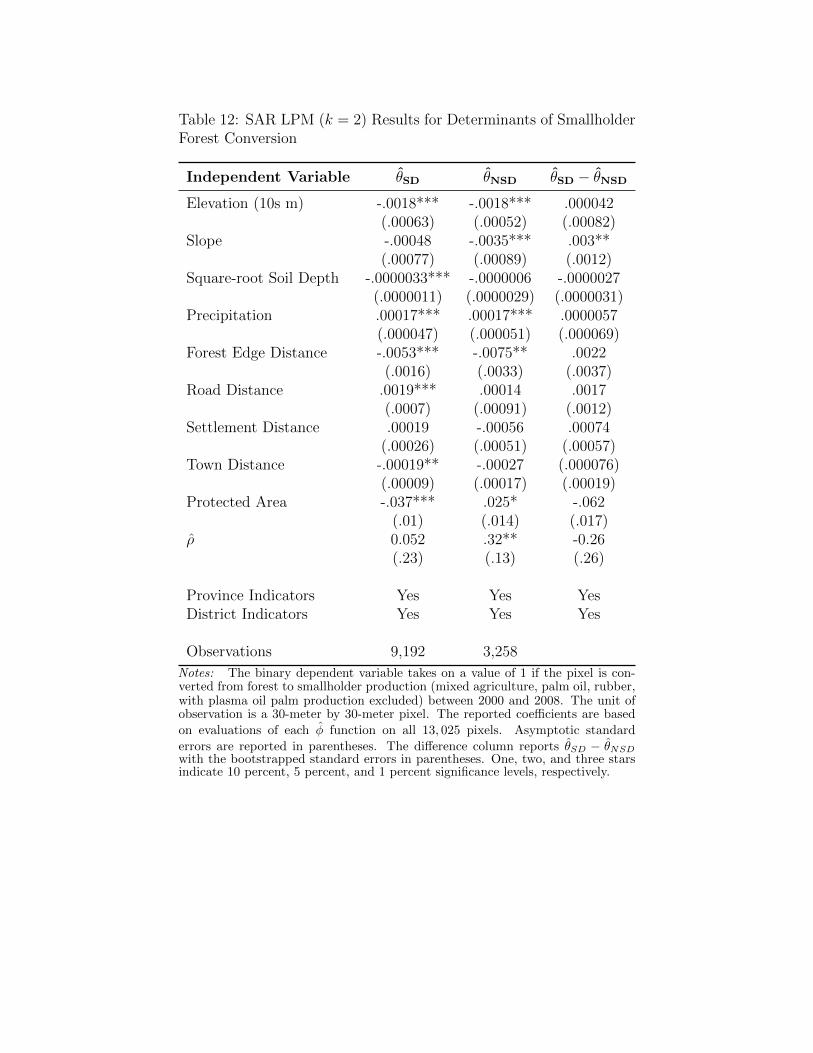
Table 12: SAR LPM (k = 2) Results for Determinants of SmallholderForest Conversion

Independent Variable θSD θNSD θSD − θNSD

Elevation (10s m) -.0018*** -.0018*** .000042(.00063) (.00052) (.00082)

Slope -.00048 -.0035*** .003**(.00077) (.00089) (.0012)

Square-root Soil Depth -.0000033*** -.0000006 -.0000027(.0000011) (.0000029) (.0000031)

Precipitation .00017*** .00017*** .0000057(.000047) (.000051) (.000069)

Forest Edge Distance -.0053*** -.0075** .0022(.0016) (.0033) (.0037)

Road Distance .0019*** .00014 .0017(.0007) (.00091) (.0012)

Settlement Distance .00019 -.00056 .00074(.00026) (.00051) (.00057)

Town Distance -.00019** -.00027 (.000076)(.00009) (.00017) (.00019)

Protected Area -.037*** .025* -.062(.01) (.014) (.017)

ρ 0.052 .32** -0.26(.23) (.13) (.26)

Province Indicators Yes Yes YesDistrict Indicators Yes Yes Yes

Observations 9,192 3,258

Notes: The binary dependent variable takes on a value of 1 if the pixel is con-verted from forest to smallholder production (mixed agriculture, palm oil, rubber,with plasma oil palm production excluded) between 2000 and 2008. The unit ofobservation is a 30-meter by 30-meter pixel. The reported coefficients are based

on evaluations of each φ function on all 13, 025 pixels. Asymptotic standard

errors are reported in parentheses. The difference column reports θSD − θNSDwith the bootstrapped standard errors in parentheses. One, two, and three starsindicate 10 percent, 5 percent, and 1 percent significance levels, respectively.

9.4 Bandwidth selection

Table 13: Optimal bandwidths for binary and multinomial nonparametric models.

Binary Multinomial

Variable Subdivided Non-subdivided Subdivided Non-subdividedConversion 0.003417204 0.006317783 0.004966546 0.00861Elevation (10s m) 5.88E+00 25020140 8.437085 4.409206Slope (percent) 1.49E+07 11.62745 7.197138 5320717Square-root Soil Depth (mm) 5186197231 4610.643 4482.164 2547.73Precipitation (km) 27.18313 29.88205 21.99456 111721695Forest Edge Distance (km) 0.5643313 0.3404008 0.6046659 0.4188318Road Distance (km) 0.5918519 0.9241033 0.6263591 1.532027Settlement Distance (km) 2.161359 0.8394453 1.957415 1.075925Town Distance (km) 0.9639768 5.252566 0.8906773 1.064054

Notes: The bandwidths are chosen for the binary nonparametric model excluding plasma production and the multi-nomial nonparametric model including plasma production. Bandwidths for the other models under consideration areavailable upon request.

Figure 1: Study areaFigure 2: Forest cover time seriesFigure 3: Location of randomly-selected pixels and district subdivision statusFigure 4: Binomial smallholder conversion probability by forest edge distanceFigure 5: Binomial smallholder conversion probability derivative by forest edge distanceFigure 6: Binomial smallholder conversion by road distanceFigure 7: Binomial smallholder conversion probability derivative by road distanceFigure 8: Smallholder oil palm conversion probability by forest edge distanceFigure 9: Model specificity and sensitivity for nonparametric modelFigure 10: Model specificity and sensitivity for spatial lpmFigure 11: Model specificity and sensitivity for logit model

Notes1Fisman (2001) uses an event-study approach to explore the value of political connections to Indonesian

firms from 1995-1997, finding that political connections may be responsible for a large-percentage of a well-connected firm’s value.

2Oil palm plantations developed a particular means of incorporating smallholders into plantation pro-duction systems through the nuclear estate scheme (McCarthy and Cramb, 2009), which follows a protocolsupported by the World Bank and other sources of capital (Little and Watts, 1994). Under this arrange-ment, plantations gain access to land that was under the de facto control of local landholders and allowthese individuals to manage small areas of oil palm that had been planted by the plantation manager withan understanding that the smallholders would sell their output solely to their affiliated plantation (referredto as plasma operations) (Levang, 2003). These arrangements subject smallholders to monopsony conditionsand the plantations tend to operate with limited transparency, leading to smaller than expected paymentsand a lack of clarity about when, if ever, the land would be returned to smallholder control (McCarthy, 2007;Potter, 1999).

3The choice of forest conversion is a dynamic problem; however, we can explore the issue in a staticcontext by making an assumption about the decision rule used to determine the timing of forest conversion.If we assume that the deforestation choice (i.e., whether or not to deforest a patch at time t conditional onthe plot being forested at this point) can be reduced to comparing the benefits from having the plot remainin forest relative to those of deforestation in time t+ 1, then the conversion choice can be studied as a staticproblem.

4There is no evidence to motivate a specific relationship between yield and forest-edge distance. Weproceed by assuming that the relationship between profit and forest-edge distance is driven by the relationshipbetween cost and distance from the forest edge (namely, π′(d) ≤ 0).

5This data is available for download from (http://www.fao.org/geonetwork/srv/en/main.home)6These cells include 4, 444 30-meter by 30-meter pixels and cover an area of 400 hectares, which is 20

times larger than the maximum smallholder production system of 20 hectares.7Estimating the impact of district subdivision may be complicated by the possibility that forests in

these districts have characteristics that make conversion undesirable. Table 9 in the appendix displays thenormalized differences, the difference in means between subdivided and non-subdivided districts divided bythe square root of the sum of the variances across both district types (Rosenbaum and Rubin, 1985; Stuart,2010), of our observable characteristics, showing that they are quite similar in both the full sample and thesample of pixels within five kilometers of a district with the other subdivision status (Imbens and Wooldridge,2009; Rubin, 2001).

8All code was written in Matlab and is available upon request. We would also direct the reader to theNP package in R as described in Hayfield and Racine (2008).

9The results of each of the inconsistent parametric models are presented in tables 10-12 in the appendix.

52

10The possibility that protected areas serve as a refuge from plantations when facing a high threat ofplantation conversion could explain the heterogeneous effectiveness of protected areas in addressing issuesof conservation and poverty that have been reported in the literature (e.g., Ferraro et al. (2011)).

11These results are depicted in table 7 in the appendix.12Table 13 presents the optimal bandwidth for the various explanatory variables in the binary and multi-

nomial analyses.13There is a substantial amount of carbon stored in the above- and below-ground biomass of tropical forests

that is released as CO2 when forests are burned prior to agricultural production. Furthermore, some tropicalforests are located on peat soil, which releases methane into the atmosphere when these areas are drainedand burned prior to production. In addition to the global damages associated with the release of thesegases, the inefficient conversion of tropical forests may lead to costs that are borne by the local populationsthrough reduced provision of valuable ecosystem services. Several of the ecosystem services provided bytropical forests are lost with forest conversion, leading to reduced water quality (Douglas, 1996), increasedand more damaging flooding events (Costa et al., 2003), changes in local climate regimes that might affectcrop yield (Costa and Foley, 2000), as well as the reduction in habitat for endemic animal and plant species(Pimm and Raven, 2000).

14While the valuation of ecosystem services is theoretically straightforward, there are a number of practicalchallenges that make the implementation of these techniques difficult (Conte, 2013). Furthermore, mappingthe provision of ecosystem services is a challenging, and data-intense task, even when efforts are made todescribe the biophysical processes in accessible ways (Kareiva et al., 2011).

15Pindyck (2013) details the numerous challenges associated with accurate estimation of the SCC.16These values are calculated using the average additional metric tons of carbon per hectare ($44.14),

converting it to dry biomass (multiplying by 0.5), then converting it to metric tons of CO2 (multiplying by3.67) and finally multiplying it by the three different estimates of the SCC.

17Deininger and Minten (2002) finds no impact of property rights after controlling for biophysical factors.18Given that our nonparametric estimates substantially outperform all of the alternative parametric models

under consideration, loss of consistency is not a valid concern in our case, which differs meaningfully fromthe conditions explored in Hall (1987a) and Hall (1987b). See figures 9-11 for a graphical representation ofrelative performance.

19It is well known that truncation error for the central-difference approximation is O(τ2). τ is chosen tobe 1× 10−12 which is smaller than the relative error due to rounding in floating point arithmetic.

53