Accepted Manuscript

Distributional impact of carbon pricing in Chinese provinces

Qian Wang, Klaus Hubacek, Kuishuang Feng, Lin Guo, KunZhang, Jinjun Xue, Qiao-Mei Liang

PII: S0140-9883(19)30109-4DOI: https://doi.org/10.1016/j.eneco.2019.04.003Reference: ENEECO 4357

To appear in: Energy Economics

Received date: 23 April 2018Revised date: 30 March 2019Accepted date: 1 April 2019

Please cite this article as: Q. Wang, K. Hubacek, K. Feng, et al., Distributional impactof carbon pricing in Chinese provinces, Energy Economics, https://doi.org/10.1016/j.eneco.2019.04.003

This is a PDF file of an unedited manuscript that has been accepted for publication. Asa service to our customers we are providing this early version of the manuscript. Themanuscript will undergo copyediting, typesetting, and review of the resulting proof beforeit is published in its final form. Please note that during the production process errors maybe discovered which could affect the content, and all legal disclaimers that apply to thejournal pertain.

ACC

EPTE

D M

ANU

SCR

IPT

Distributional impact of carbon pricing in Chinese

provinces

Qian Wang a,b

, Klaus Hubacekc,d,e

, Kuishuang Fengf,g

*, Lin Guoh, Kun Zhang

b,i, Jinjun Xue

j,

Qiao-Mei Liangb,i

**

a China Development Institute, Post-Doctoral Research Working Station, Shenzhen, 518029, China;

b Center for Energy and Environmental Policy Research, Beijing Institute of Technology, Beijing 100081, China;

c Center for Energy and Environmental Sciences (IVEM), Energy and Sustainability Research Institute Groningen

(ESRIG), University of Groningen, Groningen, 9747 AG, the Netherlands

d Department of Environmental Studies, Masaryk University, Jostova 10, 602 00 Brno, Czech Republic

e International Institute for Applied Systems Analysis, Schlossplatz 1 - A-2361 Laxenburg, Austria

f Institutes of Science and Development, Chinese Academy of Sciences, Beijing 100190, China

g Department of Geographical Sciences, University of Maryland, College Park, Maryland 21044, USA;

h School of International Trade and Economics, University of International Business and Economics, Beijing

100029, China;

i School of Management and Economics, Beijing Institute of Technology, Beijing 100081, China)

j Graduate School of Economics, Nagoya University, Nagoya 4648601, Japan

* Corresponding author: fengkuishuang@gmail.com

** Corresponding author: lqmhl@hotmail.com

Abstract: Based on a Multi-Regional Input-Output (MRIO) model, and combined with the 2012

MRIO table for 30 Chinese provinces, this paper analyzes the distributional impacts of carbon

pricing on households within and across Chinese provinces. The results show regressive

distributional effects of carbon pricing across provinces, i.e. poor provinces are affected more by

the price. Carbon pricing also shows rural-urban regressivity (i.e. rural households are impacted

more heavily than urban households) in more than half of the provinces. Within each selected

province, carbon pricing has mostly regressive effects, i.e. poorer households groups are affected

more than richer groups for urban households in all provinces and for rural houeholds in one

third of the provinces. When looking more specifically at direct energy consumption, we find

that the carbon pricing on domestic fuels generally shows regressivity, while pricing carbon on

transport fuels shows progressivity. In addition, the impact of carbon pricing on residence

(mainly on electricity and coal) is the most important contributor to the regional regressivity

across provinces.

Keywords: Carbon pricing; carbon tax; income distribution; inequality; climate change;

Input-output analysis

ACCEPTED MANUSCRIPT

ACC

EPTE

D M

ANU

SCR

IPT

1. Introduction

China has experienced fast economic growth with a rapid increase of energy consumption

and CO2 emissions over the past four decades (Feng et al., 2013). At the same time, its carbon

intensity is still much larger than the carbon intensity of developed countries and the world

average, due to large share of coal in China’s energy mix (Minx et al., 2011). Moreover, when

comparing per capita GDP across 31 provinces in 2017 (see Appendix Fig. A.1), China has

significant income differences between provinces, in particular a big gap between coastal and

inland provinces; in addition, China’s urban-rural dual economic structure leads to pronounced

inequality between rural and urban households. According to China Statistical Yearbook 2018

(NBS, 2018), in 2017, the average per capita disposable income of urban households was 36.4

thousand Yuan, while the average per capita disposable income of rural households was only

about a third with 13.4 thousand Yuan. Moreover, the urban-rural gap shows significant

differences across provinces. For example, in 2017, the per capita disposable income of Tianjin’s

urban residents was 1.85 times of its rural residents while the figure in Gansu was about 3.44

times.

These issues constitute a complex situation with potentially contradictory goals for the

Chinese government, which, on one hand strives to maintain economic growth and mitigate the

regional imbalance and income disparity, and on the other hand, attempts to realize energy

conservation and emissions reduction to address climate change. To address climate change, the

Chinese government has announced a series of emission reduction targets and declared the

implementation of climate mitigation policies, such as carbon pricing to realize these targets. For

example, China pledged to peak its CO2 emissions around the year 2030 and potentially before

that, and to reduce its carbon intensity by 60%-65% from the levels in 2005. To achieve its

carbon pricing policy, China established seven pilot carbon markets in five cities and two

provinces from 2013 to 2014, and launched the national carbon market for power generation

industry in December 19, 20171; in addition, a carbon tax policy also is planned to come into

effect as a complement to the carbon market after 20202. Many economists and scholars support

the implementation of the carbon tax in China due to its simplicity and transparency (Feng et al.,

2010; Liang and Wei, 2012).

However, the implementation of carbon pricing may cause negative distributional effects.

Due to differences in income and consumption patterns, different households groups would be

impacted differently to the same stimuli. The concern that the carbon burden will fall more

heavily on the poor is seen as a major obstacle to its policy acceptability because poor people

often spend a larger share of income on energy-intensive products to meet their basic needs (e.g.

1 People's Daily Online. National Development and Reform Commission: China has officially launched the national carbon emissions trading system. 2017-12-19. Available from:

http://finance.people.com.cn/n1/2017/1219/c1004-29716952.html. 2 China Development. Is the carbon tax really coming? 2017-10-28. Available from: http://www.chinadevelopment.com.cn/news/ny/2016/10/1092535.shtml

ACCEPTED MANUSCRIPT

ACC

EPTE

D M

ANU

SCR

IPT

heating, cooking, electricity) and lack options for substitution (Wang et al., 2016; Feng et al.,

2018). Therefore, for China, which is experiencing its transition period and meanwhile facing the

challenge of regional and urban-rural income disparities, distributional impact is a particularly

important issue which affects the social equity and justice. Assessing the distributional impact of

carbon pricing in China can provide useful information for policy makers to help them better

design the policy.

Carbon pricing attempts to internalize the external costs of carbon emissions into market

prices and to provide an incentive to mitigate carbon emissions (Wang et al., 2016). There are

two main types of carbon pricing: emissions trading systems (ETS) and carbon taxes (CT)(CPL,

2016). While numerous studies have focused on potential distributional issues of carbon pricing,

most studies have focused on developed countries (Wang et al., 2016). Although several studies

show that taxing carbon in certain developed countries/regions may be neutral (Symons et al.,

2000; Creedy and Sleeman, 2006) or weakly progressive (Tiezzi, 2005; Oladosu and Rose, 2007;

Sajeewani et al., 2015), more studies show that without carbon revenue recycling, a CT policy is

regressive in most cases (Speck, 1999; Baranzini et al., 2000; Brännlund and Nordström, 2004;

Wier et al., 2005; Kerkhof et al., 2008; Callan et al., 2009; Feng et al., 2010; Bureau, 2011; IPCC,

2014; Mathur and Morris, 2014). Regressivity means that the cost of a carbon tax to the income

or welfare of lower income groups is higher than the higher income groups, or in other words,

the burden of carbon pricing on the poor is higher than on the rich. A potential regressive effect

will aggravate inequality of a society (Feng et al., 2010; Büchs and Schnepf, 2013; Dennig et al.,

2015). As for developing countries, there are much fewer studies, some of which show

regressivity and some do not (Wang et al., 2016). Moreover, these studies show that the design

on how the CT tax is implemented and how its revenue is recycled, could affect the distributional

impact of CT (Zhang and Baranzini, 2004; Oladosu and Rose, 2007; Parry, 2015; Wang et al.,

2016). Although research has paid less attention to the distributional effect of carbon emissions

trading, they generally support the conclusion that ETS has a similar regressive effect as CT

(Parry, 2004; Burtraw et al., 2009; Shammin and Bullard, 2009). For example, Burtraw et al.

(2009) argued that through auctioning the emissions allowances and returning the auction

revenues to households, the adverse distributional impact of ETS could be altered.

Overall, existing studies on carbon pricing mainly focus on the distributional effect within a

country or a region, such as across income groups (Callan et al., 2009; Feng et al., 2010; Bureau,

2011; Mathur and Morris, 2014), between rural and urban households (Callan et al., 2009;

Bureau, 2011; Pashardes et al., 2014), among households grouped by other demographic

characteristics (e.g. family size (Wier et al., 2005; Callan et al., 2009) or households’

socio-economic status (Feng et al., 2010)), but very few pay attention to the analysis from a

multi-regional perspective.

As for China, there are several studies on the distributional impact of a hypothetical carbon

ACCEPTED MANUSCRIPT

ACC

EPTE

D M

ANU

SCR

IPT

price in China, e.g. on China’s urban-rural gap (Liang and Wei, 2012); among different income

groups (Brenner et al., 2007; Wang, 2009), or on a specific region such as Shanghai (Jiang and

Shao, 2014). On the whole, studies paying attention to the distributional impact of carbon pricing

between groups across different regions are lacking, which is exactly the contribution of this

paper. This study aims to capture the details that a national-level or a single region analysis could

not obtain, in order to put forward policy recommendations to policymakers on how to mitigate

potential unintended adverse distributional effects of carbon pricing while maintaining the

intended emission reduction effect. Given that both CT and ETS mechanisms ripple throughout

the economic system by increasing the price of fossil fuels, these two carbon pricing polices

share a a number of similarities in terms of distributional effects, we believe that our analysis

will hold for both carbon pricing instruments.

This study, therefore, focuses on analyzing the distributional impact of a certain carbon

price on the households across different regions, through answering the following 3 research

questions: (1) How will the carbon pricing impact regional inequality? (2) How will the carbon

pricing impact rural and urban households within a region? (3) Will carbon pricing enlarge the

inequality across income groups?

2 Materials and Methods

Adopting similar approaches used by Wier et al. (2005), Kerkhof et al. (2008), Feng et al.

(2010), we carry out analysis based on Multi-Regional Input-Output (MRIO ) analysis to assess

the impact of carbon pricing on households across China’s 30 provinces. Fig. A.2 illustrates the

research framework of this study.

2.1 Multi-regional input-output analysis

Multi-regional input-output (MRIO) analysis is a popular approach for analyzing the

interactions among regions and sectors and thus can account for the carbon footprint for various

economic agents (Liu et al., 2015). Therefore, MRIO method has been widely applied in energy

& environment and ecological system research, with a focus on topics such as carbon emission

accounting and decomposition analysis of driving factors (Guan et al., 2008; Su et al., 2013; Liu

et al., 2015; Fan et al., 2016), virtual water flows (Lenzen et al., 2013; Feng et al., 2014), land

use (Weinzettel et al., 2013; Yu et al., 2013), toxins (Koh et al., 2016), and a wide range of other

environmental indicators.

The MRIO model is an extension from the standard IO model to a larger economy that

includes each industry in each country or region possessing a separate row and column. The

basic equation of the IO model is shown in Eq. 1

+ = AX Y X (1)

where (in a n-sector economy):

X ~ total output vector with n dimensions whose element Xi is the output of sector i;

ACCEPTED MANUSCRIPT

ACC

EPTE

D M

ANU

SCR

IPT

Y ~ final demand vector with n dimensions whose element Yi denotes final demand

(including household and government consumption, investment, and exports) for goods i;

A ~ direct requirements matrix (or technology matrix) with n*n dimensions whose element

aij represent the direct requirements of sector j on sector i per unit output of sector j.

For MRIO model, Eq. (1) could be rewritten as Eq. (2):

11 12 1 1 1 1

21 22 2 2 2 2

1

1 2

n v

n vn

v

n n nn n nv n

Α A A X Y X

A A A X Y X

A A A X Y X

(2)

Where,

11 12 1

21 22 2

1 2

n

n

n n nn

Α A A

A A AA

A A A

, whose submatrix rn

A is m by m matrix with each element rnija

representing the volume of commodity i in region r directly required to produce per unit output of

sector j in region n; i=1, 2, …, m; j=1, 2, …, m;

1

2

n

X

XX

X

, whose submatrix r

X is a column vector with m dimensions; and its element

r

ix representing the output of sector i in region r.

The submatrix rv

Y of the final demand vector

1

2

v

v

nv

Y

Y

Y

is a column vector with m

dimensions whose element rviy denotes the sum of final demand of all items (including

household and government consumption, investment, and exports)3 for commodity i in region v

from region r.

Equations (3) can be obtained from Eq. (2).

-1

= - =X I A Y LY (3)

where,

3 Actually, when computing the result, this study disaggregate the final demand into household consumption,

government consumption, investment, and exports; and the household consumption of each region can be further disaggregated into rural households and urban households consumption; moreover, the consumption expenditures of each rural households and urban households can be divided into different income brackets.

ACCEPTED MANUSCRIPT

ACC

EPTE

D M

ANU

SCR

IPT

I ~ m*n dimension identity matrix;

1

=

L I - A ~ m*n dimension Leontief inverse matrix or total requirements matrix

whose element rnijl represents the total volume of commodity i in region r required both directly

and indirectly to produce one unit of final demand of commodity j in region n.

As shown in Eq. (4), total requirements matrix can be decomposed into three parts: I, A and

2 3 n A A A . Of them, I denotes the unit final use produced by the m*n production

sectors; A denotes the direct requirements matrix used by producing the unit final use;

2 3 n A A A denotes the total indirect requirements matrix used by producing the unit

final use. Therefore, Eq. (4) can comprehensively reflect the change in the total output of this

sector and other sectors directly and indirectly induced by the change in the final demand of any

sectors (Liang, 2007).

1 2 3( ) n L I A I A A A A (4)

2.2 Direct and indirect effects from pricing carbon

Through charging CO2 emissions from fossil fuel combustion by households and industries,

carbon pricing can reduce fossil fuel consumption and related emissions. The aim of this study is

to measure and compare the impact of carbon pricing on households among different regions, so

we focus only on households. Direct effects refers to charging direct emissions produced by

households such as cooking, heating and driving; indirect effects refer to charging indirect

emissions arising throughout the production steps required to produce households’ final

consumption items. Given that pricing carbon on fossil fuel consumption will lead to different

prices of products, and different consumers have different consumption structures, the final tax

burden may be unevenly distributed (Wang, 2009). Therefore, it is necessary to undertake a

comparative analysis on the carbon pricing burden of different household groups between and

within regions.

Consistent with existing studies (Wier et al., 2005; Kerkhof et al., 2008; Feng et al., 2010,

2018), this study also assumes that the carbon pricing burden imposed on production sectors can

be fully passed onto the consumers, therefore, households bear both the direct and indirect

impact by the carbon pricing. This approach ignores demand elasticities and substitution

possibilities, which is a common shortcoming of these type of studies. The IO method can

calculate the indirect emissions driven by final demand thus captures the indirect effect of carbon

pricing. In this study, given our interest in impacts on households, we only focus on household

consumption.

The total carbon payment of consumption category k is the sum of direct and indirect

carbon payments.

ACCEPTED MANUSCRIPT

ACC

EPTE

D M

ANU

SCR

IPT

_ _k k kCT CT d CT nd (5)

Where, _ kCT d , _ kCT nd and kCT represent the direct, indirect, and total carbon

(pricing) payment on consumption category k, respectively. When setting the carbon price as t

Yuan/t CO2, kCT can be obtained through Eq. (6).

( _ _ )k k kCT E d E nd t (6)

Where, _ kE d , _ kE nd denote the direct and indirect emissions due to the consumption

on category k, respectively. Then production emissions coefficient Ck can be calculated by

dividing the direct emissions of sector k by its total output.

Then, for the MRIO model, the indirect emissions coefficient matrix driven by final

consumption is CL, where

11

22

nn

C

CC

C

, and submatrix rrC is a m by m diagonal

matrix whose element rriiC denotes the production emissions coefficient of sector i in region r.

The indirect emissions vector driven by household h in region v can be obtained through Eq. 7:

1 111 11 12 1

2 222 21 22 2

1 2

v vn

h h

v vn

h h

nn n n nnnv nv

h h

_

_

_

E nd YC L L L

E nd YC L L L

C L L LE nd Y

(7)

And the total indirect emissions driven by household h in region v can be obtained by Eq. 8:

1 1

_ _n m

v rv

h ih

r i

E nd E nd

(8)

2.3 Selection of indicators

To answer the three questions mentioned in the introduction section, two types of indicators

are selected in this study. One category is used to measure how heavy the carbon pricing burden

is: 1) absolute value of per capita carbon payment and 2) the per capita carbon payment burden

rate. The per capita carbon payment is the average cost per person paid for his/her own carbon

emissions. And, the per capita carbon pricing burden rate refers to the percentage of per capita

carbon payment in the per capita expenditure which is the sum of the pre-tax per capita

expenditure and the per capita total carbon payment. The second category indicates if the carbon

pricing will exacerbate the regional imbalance. Here we choose the Suits index (Suits, 1977) to

ACCEPTED MANUSCRIPT

ACC

EPTE

D M

ANU

SCR

IPT

measure the distributional effect of carbon pricing.

The Suits index has been widely used to measure the distributional effect of a tax or public

expenditure, including environmental taxes (Metcalf, 1999), vehicle pollution control policies

(West, 2004), gasoline taxes (Agostini and Jiménez, 2015), and carbon taxes (Wier et al., 2005;

Jiang and Shao, 2014). The index ranges from +1, i.e. extreme progressivity, where the entire tax

burden is borne by members of the highest income bracket, through 0 for a proportional tax, to –

1, which refers to extreme regressivity, at which the entire tax burden is borne by members of the

lowest income bracket (Suits, 1977).

The calculation of Suits index is based on the idea of the Gini coefficient and the Lorenz

curve (referred to as concentration curve by Suits). Fig. 1 shows an example of the concentration

curve. The horizontal axis represents the accumulated percent of the income and the accumulated

percent of the tax burden is plotted vertically. The population is ranked by income from low to

high.

Fig.1 The schematic diagram of the Suits index

Following Suits (1977), the Suits index (S) can be calculated through Eq. 9:

/ 1 /S K L K L K (9)

Where K is the area of the triangle OAB in Fig. 1, L is the area OABC between the curve and the

horizontal axis OA. And L can be obtained through Eq. 10.

1

0

1 1

1

( )

(1/ 2)[ ( ) ( )]( )n

i i i i

i

L T r dr

T r T r r r

(10)

Where ri denotes the accumulated percent of income of the ith

group, measured on the

horizontal axis, which ranges from 0 to 1; T(ri) is the corresponding accumulated percent of the

tax burden borne by the ith

group, and n stands for the number of households’ income groups.

For 0 0r , 0( ) 0T r , K=1/2, the Suits index can be approximately obtained through Eq. 11.

ACCEPTED MANUSCRIPT

ACC

EPTE

D M

ANU

SCR

IPT

1 1

1

1 2 1 [ ( ) ( )]( )n

i i i i

i

S L T r T r r r

(11)

2.4 Data source and data processing

The data source for this study is China’s MRIO table for 2012 with 42 sectors in 30 provinces

(excluding Tibet). Emissions data are taken from the China’s provincial and national emissions

inventory for 2012 provided by China Emission Accounts and Datasets (CEADs)4. In this study,

we only focus on the CO2 emissions associated with fossil fuels, thus the process emissions (e.g.

emissions from cement production) are not included. Population data are taken from the China

Statistical Yearbook 2013 (NBS, 2013).

Data processing for production emissions coefficients: CEADs emissions data includes 45

sectors while the sector number of MRIO is 42. Su et al. (2010) summarized two data treatment

schemes to make the sector numbers between emissions coefficient and the Leontief inverse

matrix compatible. The first is to aggregate the finer IO data to the level that matches the energy

consumption data, while the other is to disaggregate the energy consumption data to the level that

matches the IO data. We used both approaches to match the datasets and calculate production

emissions intensity coefficients for 42 sectors in each of 30 provinces in China for the year 2012.

The concordance matrix linking the datasets is shown in Appendix Table A.1.

Disaggregation of different income groups within provinces: In order to capture the

differences of carbon pricing burden between different household groups, we need to further

disaggregate urban and rural households in 30 provinces of MRIO to the level of different

income groups. The per capita annual consumption expenditure survey data for different urban

and rural income groups in each province are taken from China provincial statistical yearbook

2013 for 30 provinces. The relationship between household consumption expenditure items and

products of MRIO sectors is shown in Appendix Table A.2.

Since some provinces do not provide detailed data on households’ expenditure at the level

of income groups, we also illustrate the data availability in Fig.25. Specifically, the area marked

by star indicates that the data are available for both rural and urban income groups in that

province; areas marked with triangle denote that only the data on urban income groups are

available; and the provinces with cross label represent that data are unavailable for both rural and

urban income groups. In addition, there are also some regions, such as Tibet, Taiwan, Hong

Kong and Macau, which are not discussed in this study due to data limitations. Finally, 12

provinces with star label (Beijing, Heilongjiang, Shanghai, Zhejiang, Jiangsu, Henan, Jiangxi,

Guangdong, Fujian, Guangxi, Chongqing, Gansu) are divided into different income groups

within both rural and urban areas, while another 12 provinces marked with triangle (Tianjin, Jilin,

4 China Emission Accounts and Datasets (CEADs): http://www.ceads.net/data/inventory-by-sectoral-approach/. 5 Taking into account the possible similarity between neighboring provinces, we aggregate the 30 provinces in Fig.2 to eight regions according to geographical characteristics.

ACCEPTED MANUSCRIPT

ACC

EPTE

D M

ANU

SCR

IPT

Liaoning, Anhui, Hubei, Hainan, Sichuan, Inner Mongolia, Shaanxi, Qinghai, Ningxia, Xinjiang)

are divided into different income groups only within the urban.

ACCEPTED MANUSCRIPT

ACCEPTED MANUSCRIPT

Fig. 2 Eight economic regions in mainland China

ACCEPTED MANUSCRIPT

ACC

EPTE

D M

ANU

SCR

IPT

2.5 Carbon pricing schemes

According to a preliminary estimates of the National Development and Reform

Commission, in the long run, a carbon price of 300 Yuan /t CO2 is regarded as a price standard

which can play a role in leading the low-carbon green development6. From the experience of

China’s 7 pilot carbon markets, the average carbon price ranges from 10 to 50 Yuan /t CO27.

Considering that a higher carbon price might lead to a heavier economic burden to industries and

households, some studies suggest a lower rate ranging from 10~20 Yuan/t CO2 (Su et al., 2011;

Jiang and Shao, 2014). As a compromise (but not as a suggestion), we set the carbon price at 50

Yuan /t CO2, and added a low carbon price scenario at 10 Yuan /t CO2 and a high carbon price

scenario at 100 Yuan /t CO2 to construct a sensitivity analysis.

In this paper, all carbon pricing revenues are not recycled back to the economy, which also

means that no social protection measures are considered.

2.6 Limitations

This study estimates the short-term distributional impacts of carbon pricing from an

expenditure-side perspective, which means that the income changes of households due to the

carbon pricing are not modeled; meanwhile, as mentioned in Feng et al. (2010), the behavioral

response of consumers to higher prices and the associated changes in production are not

considered within the current IO model framework. In fact, carbon pricing will affect household

income through affecting the input of production factors and thereby the factor incomes such as

wages and returns to capital (Feng et al. 2010; Liang and Wei, 2012; Liang et al., 2013).

Meanwhile, in the long run, the production structure and production technology will change

significantly, but these can be simulated only by more complicated models like computable

general equilibrium (CGE) models. However, production structures and consumption patterns

can be rather inflexible in the short run and thus the input-output approach provides a useful first

approximation of short-run impacts and can put forward helpful information for policy makers

on the fairness of carbon pricing mechanisms, and allows to model and develop different

measures to mitigate the regional regressivity of carbon pricing.

3 Results

3.1 Comparison of household’s carbon burden for 30 provinces in China

If the implementation of carbon pricing mechanism makes the less developed regions (with

low per capita GDP) bear a higher carbon burden than those developed regions (with high per

capita GDP), we define carbon pricing as regressive. Fig. 3 shows the carbon payment burden

rate of residents in China’s 30 provinces.

6 Economic Information Daily. The construction of the carbon market trading system enters the sprint period. 2017-10-30. Available from: http://www.jjckb.cn/2016-10/31/c_135792422.htm 7 China Carbon Emissions Trading Network. 2018-1-30. Available from: http://www.tanpaifang.com/

ACCEPTED MANUSCRIPT

ACC

EPTE

D M

ANU

SCR

IPT

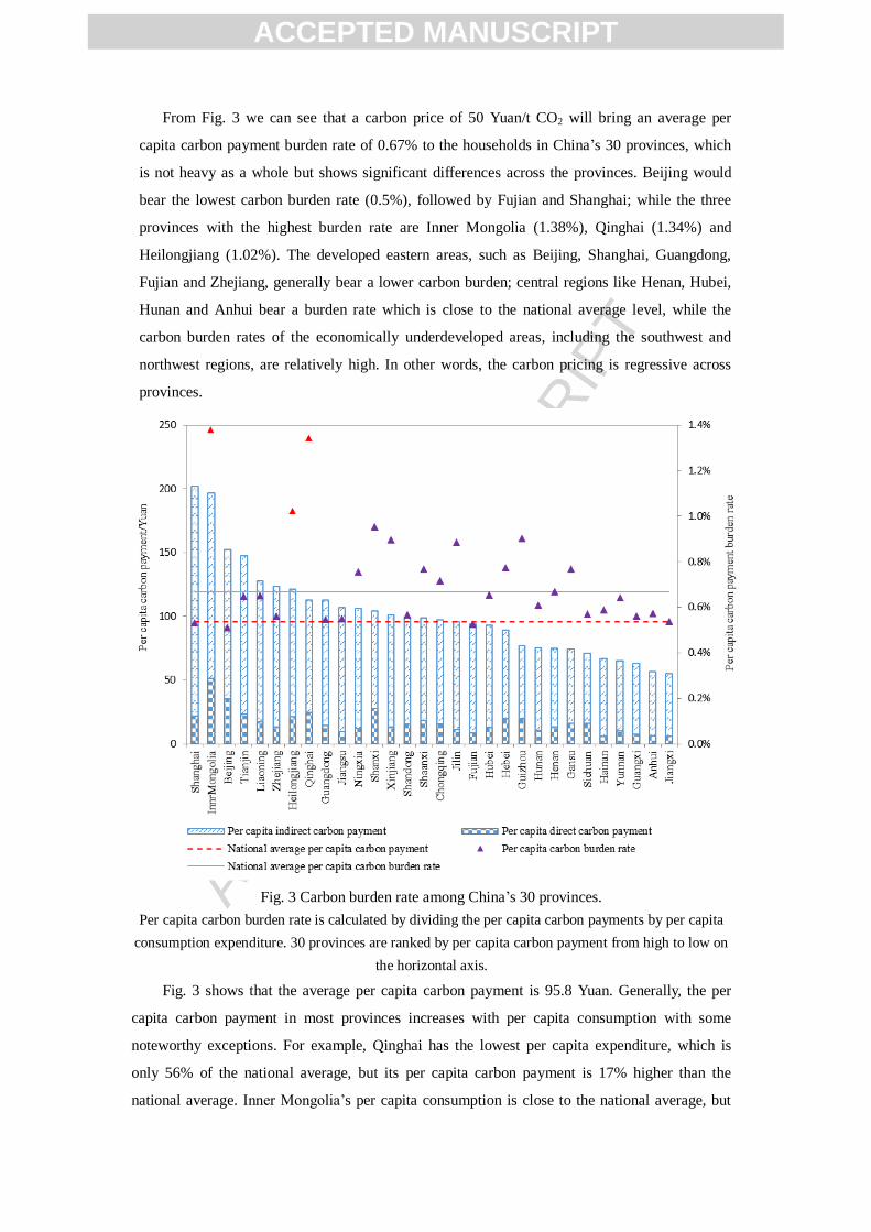
From Fig. 3 we can see that a carbon price of 50 Yuan/t CO2 will bring an average per

capita carbon payment burden rate of 0.67% to the households in China’s 30 provinces, which

is not heavy as a whole but shows significant differences across the provinces. Beijing would

bear the lowest carbon burden rate (0.5%), followed by Fujian and Shanghai; while the three

provinces with the highest burden rate are Inner Mongolia (1.38%), Qinghai (1.34%) and

Heilongjiang (1.02%). The developed eastern areas, such as Beijing, Shanghai, Guangdong,

Fujian and Zhejiang, generally bear a lower carbon burden; central regions like Henan, Hubei,

Hunan and Anhui bear a burden rate which is close to the national average level, while the

carbon burden rates of the economically underdeveloped areas, including the southwest and

northwest regions, are relatively high. In other words, the carbon pricing is regressive across

provinces.

Fig. 3 Carbon burden rate among China’s 30 provinces.

Per capita carbon burden rate is calculated by dividing the per capita carbon payments by per capita

consumption expenditure. 30 provinces are ranked by per capita carbon payment from high to low on

the horizontal axis.

Fig. 3 shows that the average per capita carbon payment is 95.8 Yuan. Generally, the per

capita carbon payment in most provinces increases with per capita consumption with some

noteworthy exceptions. For example, Qinghai has the lowest per capita expenditure, which is

only 56% of the national average, but its per capita carbon payment is 17% higher than the

national average. Inner Mongolia’s per capita consumption is close to the national average, but

ACCEPTED MANUSCRIPT

ACC

EPTE

D M

ANU

SCR

IPT

its per capita carbon payment is 2.1 times the national average level, which is close to Shanghai’s

per capita carbon payment level. As a result, the carbon burden rate of these two provinces is

significantly higher than that of other provinces. Shanghai’s and Beijing’s per capita carbon

payments are relatively high with 2.1 and 1.6 times the national average level, respectively. But

due to their higher per capita consumption level, which is 1.6 and 1 times higher than the

national average, their per capita carbon burden rate becomes the lowest.

Fig. 3 also shows that the characteristics of indirect per capita carbon payments for China’s

provinces are similar to the total per capita carbon payment, and also plays a dominant role in the

total per capita carbon payment. Their proportions range from 74% to 91%. Furthermore, the

direct per capita carbon payment is relatively stable across the provinces and does not show a

close correlation with per capita consumption levels. Therefore, compared with the indirect per

capita carbon payment, the direct payment is more regressive.

We analyze the differences in the carbon burden rate between provinces through

decomposing its structure as shown in Fig.4. for 8 major categories of consumer goods. The top

three contributors are Residence (which includes water, electricity, fuels and housing as shown

in Table A.2), Transportation & Communication and Food, which account for about two-thirds

of the total per capita carbon burden rate. In particular, for those provinces with a higher carbon

burden, such as Inner Mongolia, Qinghai and Heilongjiang, Residence accounts for 51.4%,

64.9% and 48.6% carbon burden rate, respectively. However, for those with low carbon burden

rates, such as Beijing, Fujian and Shanghai, the contribution of Residence to the total carbon

burden rate is only 19.4%, 28.2% and 21.8%, respectively. Therefore, Residence is the most

important contributor to the regional regressivity of carbon pricing. Moreover, by further

analyzing the structure of Residence category, as shown in Fig.A.3, we find that electricity

consumption plays a dominant role in most provinces, followed by coal and gas consumption.

ACCEPTED MANUSCRIPT

ACC

EPTE

D M

ANU

SCR

IPT

Fig.4 Per capita carbon payment burden rate by consumption categories of goods and services

3.2 Distribution of carbon burden between rural and urban households within each

province

There is a large income gap between China’s urban and rural residents. In general, the

income and expenditure level of urban residents is larger than that of rural residents. If the

implementation of carbon pricing mechanism will make rural residents bear a higher carbon

burden than urban residents, the carbon pricing is regressive, which can be called rural-urban

regressive here, and vice versa. Similarly, if carbon pricing makes the lower income groups

shoulder heavier than the higher income groups, the carbon pricing is regressive across income

groups.

We calculated the per capita direct, indirect and total carbon burden for both urban and rural

households in each of the 30 provinces. And the per capita total carbon burden rate is the sum of

per capita direct carbon burden rate and per capita indirect carbon burden rate. To highlight the

rural- urban differences, we further calculate the relative gap in carbon burden between the urban

and rural households in each province, as shown in Fig. 5.

Fig.5a shows the rural-urban relative gap caused by the total carbon pricing. We can see that

the carbon pricing are rural-urban regressive in more than half of the 30 provinces whereas a

handful of provinces show relatively weak rural-urban progressivity.

ACCEPTED MANUSCRIPT

ACC

EPTE

D M

ANU

SCR

IPT

Fig. 5 The rural-urban relative gap in carbon burden rate in each of 30 provinces. (a) Total carbon pricing; (b)

Direct carbon pricing; (c) Indirect carbon pricing. (Notes: The rural-urban relative gap is obtained through dividing

the per capita burden rate of rural households by that of urban households and minus one, thus a positive value

means that the carbon pricing is rural-urban regressive.)

The direct carbon pricing causes rural-urban regressivity to 23 of the 30 provinces (see Fig.

5b). And the regressivity is much stronger than that of the total carbon pricing and the indirect

carbon pricing. Through analyzing the three components of direct carbon pricing (coal,

petroleum and gas), we find that the carbon payment due to coal consumption show obvious

rural-urban regressivity in almost all provinces, which is the main reason for the strong

rural-urban regressivity of the direct carbon pricing. Unlike the direct carbon pricing, as shown

in Fig.5c, the indirect carbon payment brings relatively weak rural-urban progressivity to 20

provinces while causes rural-urban regressivity to the remaining 10 provinces.

3.3 Inequality of carbon tax payment

This section chooses the Suits index (see Eq. 11) to measure the distributional effects of

carbon pricing, in order to accurately reflect whether the carbon pricing will exacerbate China’s

regional imbalance and how serious it is. Table 1 shows the Suits index of carbon pricing in rural,

ACCEPTED MANUSCRIPT

ACC

EPTE

D M

ANU

SCR

IPT

urban and total households among 30 provinces. We calculate the Suits index to represent the

direct, indirect and total distributional effects of carbon pricing, respectively.

Table 1 the Suits index of carbon pricing

Suits index Direct carbon payment Indirect carbon payment Total carbon payment

Rural -0.130 -0.024 -0.049

Urban -0.132 -0.066 -0.075

National total -0.210 -0.032 -0.060

Note: The national total here only contains the 30 provinces observed in this study.

As shown in Table 1, pricing carbon on fossil energy consumption at a price of 50 Yuan/t

CO2 will have a regressive distributional effect to rural, urban and national total households

across 30 provinces. Among them, the direct carbon payment, namely, the payment due to

households’ direct carbon emissions, has a stronger regressive effect in the rural, urban and the

total households, with the regressivity in the national total being the strongest. The indirect

carbon payment, which can be understood as the cost of carbon pricing transferred from the

production sectors, shows a relatively weak regressivity.

Overall, the direct carbon pricing has the most obvious regressivity, while the indirect

carbon pricing has a relatively weak regressivity, and in total, the carbon pricing has a weak

regressivity. Moreover, the extent of regressivity for urban is somewhat stronger than for rural

households, and the regressivity within the national total households is between the extent for

rural and urban, with an exception that the national Suits index of the direct carbon payment

shows the most significant regressivity.

3.4 Comparison of carbon burden among different income groups within each province

This section wants to further explore whether the carbon pricing will have an uneven

distributional effect among different income groups within each province. As mentioned in

section 2.4, due to data limitation, only 12 provinces are divided into different income groups

within both rural and urban areas, while another 12 provinces are disaggregated only within the

urban (see Fig. 2).

And Fig.6 presents the carbon burden rate of different income groups within these

provinces.

ACCEPTED MANUSCRIPT

ACCEPTED MANUSCRIPT

Fig.6 Per capita carbon burden rate of different income groups in each province

(Notes: R1, R2, R3, R4, R5 denote different income groups of rural households from low income level to high; U1, U2, U3, U4, U5, U6, U7 represent different income groups of urban households from low income level to high.)

Per capita indirect carbon burden rate Per capita direct carbon burden rate

ACCEPTED MANUSCRIPT

ACC

EPTE

D M

ANU

SCR

IPT

Fig.6 shows that, overall, the distributional effect of uniform national carbon pricing within

urban areas in most provinces (and also within a few provinces’ rural areas) would exacerbate

income disparity in these areas. But, some areas show progressive distributional effects in that

carbon pricing burden increases with the income level, such as rural Shanghai, Fujian and

Guangxi, and urban Hainan and Sichuan, as well as urban and rural Jiangxi. Finally, although the

carbon burden rate of a national uniform carbon price is distributed unevenly across different

income groups in each area, this difference is relatively small compared with the gap between

provinces or the gap between rural and urban households in each province.

In order to obtain an accurate distributional effect of carbon pricing, we calculate the Suits

index in each region, as shown in Table A.3. Fig.2 classifies the observed 24 provinces into 7

regions, thus Table A.3 can provide results about distributional impacts of carbon pricing from

both provincial and regional levels.

For most provinces, carbon pricing has regressive distributional effects both across different

urban-rural income groups (see overall Suits index) and within urban groups themselves. While, it

shows weak progressivity in two-thirds of the 12 selected rural areas. In addition, direct carbon

payment shows much stronger regressivity than the indirect carbon payment, as a result, the total

carbon payment shows less regressivity in most provinces.

We further categorize direct energy consumption into domestic fuels (coal and gas) and

transport fuels (petroleum) according to the purpose of energy use, and calculate the Suits index of

carbon pricing on domestic fuels and on transportation fuels, respectively, as shown in the first

two columns of Table A.3. The carbon payment due to domestic fuels shows regressivity, while

the carbon payment on transport fuels shows progressivity, independent of urban-rural status.

3.5 Sensitivity analysis

In this section, sensitivity analyses are performed by setting the carbon price at 10 and 100

Yuan/t CO2, respectively. As shown in Fig. 7, the average per capita carbon burden rate caused by

carbon prices of 10, 50 and 100 Yuan/t CO2 are 0.134%, 0.667% and 1.324%, respectively. Since

the carbon payment under the carbon prices 10~100 are all much lower than the level of the

pre-tax per capita expenditure, the obtained carbon burden rate almost shows proportional increase

with the prices ranging from 10 to 100 Yuan/t CO2. In addition, we also find that the ranking of 30

provinces by the per capita carbon burden rate does not change with the increase of the carbon

price.

ACCEPTED MANUSCRIPT

ACC

EPTE

D M

ANU

SCR

IPT

Fig. 7 Provincial carbon burden rates for different carbon prices

Furthermore, we also compare the rural-urban distributional effects under different carbon

prices (10 and 100 yuan) and calculate their corresponding Suits index. Results show that no

directional changes occur in distributional impacts independent of province and income group.

Moreover, the absolute value of Suits index will decrease very slightly with an increase of carbon

price. This result is directly related to our assumption that consumer behavior does not change

immediately after the introduction of the carbon pricing policy. This hypothesis is strong in the

long term, but it is acceptable in assessing the potential short-term impact of carbon pricing.

4 Conclusions and policy implications

This study employed the MRIO model to analyze the regional distributional impact of a

national uniform carbon price in China. Based on our results we can draw several conclusions:

First, carbon pricing effects are different across provinces. The average carbon burden rate

caused by a carbon price of 50 Yuan/t CO2 is 0.67%, which is not heavy as a whole but is unevenly

distributed across provinces. Richer provinces such as Beijing, Shanghai and Guangdong bear a

lower carbon pricing burden than the poorer provinces in Western China. Meanwhile, residence

category contributes most to the regressivity of carbon pricing, and electricity and coal constitute

the main parts to direct household expenditure for heating and cooling and similar items. This

emphasizes the need to put high importance on the optimization of the energy and electricity

structure, and to a reduction of coal use, especially by households.

Second, carbon pricing shows rural-urban regressivity in more than half of the 30 provinces,

which indicates that a national uniform carbon price would widen the rural-urban gap in these

provinces. In other provinces, the carbon pricing show weak rural-urban progressivity or

approximately proportional distributional effect between rural and urban. This shows us the rural

households (especially rural low income groups which are lacking the discourse power) are the

most vulnerable groups to the potential negative impact of carbon pricing, and thus need to be paid

special attention to.

ACCEPTED MANUSCRIPT

ACC

EPTE

D M

ANU

SCR

IPT

Third, the direct effect of carbon prices shows a relatively strong regressivity for all

household categories and provinces, while the indirect effects shows relatively weak regressivity.

In total, the carbon pricing has weak regressivity for all household types and provinces.

Fourth, the carbon pricing has regressive distributional effects across different income groups

within urban households of most provinces; while for rural income groups, it is weakly

progressive in two-thirds of the 12 selected rural areas. In addition, the distributional impact of

direct carbon payments is regressive in most provinces, and the extent of such regressivity is

stronger than that of the indirect carbon payment and total carbon payment.

Last, when categorizing the direct energy consumption into domestic fuels (coal and gas) and

transport fuels (petroleum), in general, the carbon pricing on domestic fuels shows regressivity,

while pricing carbon on transport fuels shows progressivity, for all households and provinces. This

result reminds policymakers that different carbon pricing policies should be designed between

domestic fuels and transport fuels. Households are very small emission sources, which are not

included in the carbon market system at present. Once a carbon tax is considered for all emission

sources that are not covered by the carbon market, we recommend households’ transportation fuels

rather than domestic fuels could be taxed first. If domestic fuels are also to be taxed for

households, extra measures for vulnerable low income groups should be taken to avoid its

potential regressive effects.

Results of this study show that carbon pricing may increase the rural-urban gap, the

provincial gap and the inequality within provinces, but overall, such a regressive distributional

impact is not strong. From the experience of China’s 7 carbon market pilots, we can see that the

overall current carbon price is still at a rather low level ranges from 10 to 50 Yuan /t CO2, which

has not created an onerous impact on economy and living standards. However, with higher future

carbon prices, the burden caused might create social hardship for lower income groups and rural

households.

Given that the current regional imbalance and income disparity have already been very large,

adequate attention should be paid to even a small regressive policy. Based on our results, we

suggest that when China gradually establishes more comprehensive carbon markets and higher

prices, measures need to be taken to mitigate potential regressive distributional impacts. For

example, the most practical way might be recycling the carbon pricing revenues to

vulnerable/low-income households of the most affected areas, or to set differential tax rates for

provinces.

Acknowledgements

The authors gratefully acknowledge financial support from the National Key R&D Program

of China (2016YFA0602603), China Postdoctoral Science Foundation (2018M643359), the

National Natural Science Foundation of China (Nos. 71461137006, 71422011, 71521002). Klaus

Hubacek was partly supported by the Czech Science Foundation under the project VEENEX (GA

ČR no. 16-17978S).

Appendix

ACCEPTED MANUSCRIPT

ACC

EPTE

D M

ANU

SCR

IPT

Fig. A.1 Per capita GDP of 31 provinces in China for 2017

(Data source: China Statistical Yearbook 2018(NBS, 2018))

The regional distributional impact of

carbon pricing

﹒Comparison among 30 provinces

﹒Comparison between the urban and

rural within 30 provinces

﹒Comparison among income groups

within 8 regions

Multi- regional

input-output (MRIO)

model

﹒MRIO table with 42

sectors for 2012

﹒CEADs emissions data

Indicators：

- Carbon payment burden

﹒Per capita carbon payment

(absolute value)

﹒Per capita carbon payment

burden rate

- Progressivity/Regressivity

﹒Suits index

﹒Rural-urban gap

﹒Regional gap

﹒Gap between income groups

﹒How heavy the burden is?

﹒Regressive or progressive？Performance

Fig. A.2 Research framework

Table A.1 The relationship between the sectors of provincial-level CO2 emission inventory from

CEADs and the sectors of MRIO table

ACCEPTED MANUSCRIPT

ACC

EPTE

D M

ANU

SCR

IPT

Sectors of Provincial-level CO2 emission inventory

from CEADs Sectors of MRIO table

Code Sector name Sector name Code

1 Farming, Forestry, Animal Husbandry, Fishery and Water Conservancy Farming, Forestry, Animal Husbandry,

Fishery Products and Services

1

8 Logging and Transport of Wood and Bamboo

2 Coal Mining and Dressing Coal Mining and Dressing Products 2

3 Petroleum and Natural Gas Extraction Petroleum and Natural Gas Extraction Products

3

4 Ferrous Metals Mining and Dressing Metals Mining and Dressing Products

4

5 Nonferrous Metals Mining and Dressing

6 Nonmetal Minerals Mining and Dressing Nonmetal Minerals and Other Minerals Mining and Dressing Products

5

7 Other Minerals Mining and Dressing

9 Food Processing Food and Tobacco 6

10 Food Production

11 Beverage Production

12 Tobacco Processing

13 Textile Industry Textile 7

14 Garments and Other Fiber Products Garments and Other Fiber Products Leather, Furs, Down and Related Products

8

15 Leather, Furs, Down and Related Products

16 Timber Processing, Bamboo, Cane, Palm Fiber & Straw Products

Wood Processing products and Furniture

9

17 Furniture Manufacturing

18 Papermaking and Paper Products Papermaking, Printing, Cultural, Educational and Sports Articles

10

19 Printing and Record Medium Reproduction

20 Cultural, Educational and Sports Articles

21 Petroleum Processing and Coking Petroleum Processing and Coking Products

11

22 Raw Chemical Materials and Chemical

Products

Chemical Products 12

23 Medical and Pharmaceutical Products

24 Chemical Fiber

25 Rubber Products

26 Plastic Products

27 Nonmetal Mineral Products Nonmetal Mineral Products 13

28 Smelting and Pressing of Ferrous Metals Smelting and Pressing of Metals

14

29 Smelting and Pressing of Nonferrous Metals

30 Metal Products Metal Products 15

31 Ordinary Machinery Ordinary Machinery 16

32 Equipment for Special Purposes Equipment for Special Purposes 17

33 Transportation Equipment Transportation Equipment 18

34 Electric Equipment and Machinery Electric Equipment and Machinery 19

35 Electronic and Telecommunications Equipment

Electronic and Telecommunications Equipment

20

36 Instruments, Meters, Cultural and Office Machinery

Instruments, Meters, Cultural and Office Machinery

21

37 Other Manufacturing Industry

Other Manufacturing Industry; Services for Metal Products, Machinery and Equipment

22, 24

38 Scrap and Waste Scrap and Waste 23

39 Production and Supply of Electric Power, Steam and Hot Water

Production and Supply of Electric Power, Steam and Hot Water

25

40 Production and Supply of Gas Production and Supply of Gas 26

41 Production and Supply of Tap Water Production and Supply of Tap Water 27

ACCEPTED MANUSCRIPT

ACC

EPTE

D M

ANU

SCR

IPT

42 Construction Construction 28

43 Transportation, Storage, Post and

Telecommunication Services Transportation, Storage and Post 30

44 Wholesale, Retail Trade and Catering Services

Wholesale, Retail Trade 29

Accommodation and Catering Services 31

45 Others

Information Transmission, Software and Information Technology Services

32

Finance 33

Real Estate 34

Leasing and Commercial Services 35

Scientific Research and Technical Services

36

Water Conservancy, Environment and

Public Facilities Management 37

Resident Services, Repairs and Other Services

38

Education 39

Health and Social Work 40

Culture, Sports and Entertainment 41

Public Management, Social security and Social Organizations

42

Table A.2 The relationship between household consumption expenditure items and the sectors of

MRIO table

Expenditure items Sectors of MRIO table

Food 1, 6

Clothing 7-8

Household Facilities, Articles and Services 9, 15-17, 19, 21

Transportation & Communication and

Food

11, 18, 20, 30, 32

Chemical & Medicine 12, 40

Recreation, Education and Cultural

Services

10, 39, 41

Residence 2, 13, 25-28, 34-35

Water, electricity and fuels 2, 25-28,

Housing 13, 34-35

Other Goods & Services 22, 24, 29, 33, 36-38, 42

Accommodation and Catering Services 31

ACCEPTED MANUSCRIPT

ACC

EPTE

D M

ANU

SCR

IPT

Fig.A.3 Structure of carbon burden rate on Residence category by 30 provinces

Table A.3 Suits index of carbon pricing

Regions Provinces Suits index

Energy domain Direct carbon

payment Indirect carbon

payment Total carbon

payment Transport fuels

Domestic fuels

Jing-Jin (JJ)

Beijing

Rural 0.0982 -0.0297 -0.0209 0.0260 0.0019

Urban 0.0640 -0.2504 -0.0409 -0.0158 -0.0208

Overall 0.0985 -0.5033 -0.1909 -0.0101 -0.0523

Tianjin Urban 0.0911 -0.1695 0.0345 -0.0392 -0.0286

Northeast (NE)

Heilongjiang

Rural 0.0556 -0.0202 0.0117 -0.0020 0.0002

Urban 0.2759 -0.3384 -0.0875 -0.0363 -0.0455

Overall 0.2222 -0.1556 -0.0003 0.0078 0.0063

Jilin Urban 0.2493 -0.1197 0.0428 -0.0436 -0.0333

Liaoning Urban 0.3109 -0.1276 0.0106 -0.0109 -0.0085

Eastern Coastal

(EC)

Shanghai

Rural 0.0526 0.0415 0.0470 0.0134 0.0244

Urban 0.0062 -0.1661 -0.0567 -0.0151 -0.0188

Overall -0.1414 -0.3429 -0.2233 -0.0171 -0.0407

Zhejiang

Rural 0.0704 -0.1087 -0.0385 0.0023 -0.0052

Urban 0.0691 -0.2720 -0.1502 -0.0279 -0.0381

Overall -0.1459 -0.3300 -0.2614 -0.0359 -0.0607

Jiangsu

Rural 0.0435 -0.0068 0.0258 -0.0024 -0.0010

Urban 0.0430 -0.1460 -0.0200 -0.0154 -0.0158

Overall 0.1026 -0.0612 0.0475 -0.0217 -0.0157

Central Region (CR)

Henan

Rural 0.0872 0.0143 0.0214 0.0023 0.0080

Urban 0.1582 -0.2281 -0.1345 -0.0354 -0.0465

Overall 0.0426 -0.3534 -0.2911 0.0114 -0.0421

ACCEPTED MANUSCRIPT

ACC

EPTE

D M

ANU

SCR

IPT

Jiangxi

Rural 0.1052 0.0596 0.0740 0.0151 0.0232

Urban 0.3144 -0.0216 0.1067 0.0185 0.0261

Overall 0.0851 -0.1384 -0.0598 0.0098 0.0026

Anhui Urban 0.2011 -0.1369 -0.0339 -0.0371 -0.0367

Hubei Urban 0.1949 -0.1181 -0.0150 -0.0070 -0.0079

Southern Coastal

(EC)

Guangdong

Rural 0.0129 -0.1431 -0.0776 0.0027 -0.0191

Urban 0.1035 -0.1494 -0.0498 -0.0145 -0.0181

Overall -0.1223 -0.2632 -0.2065 0.0027 -0.0243

Fujian

Rural 0.0621 0.0374 0.0465 0.0034 0.0098

Urban 0.1088 -0.1988 -0.0537 -0.0374 -0.0386

Overall -0.0096 -0.2517 -0.1476 -0.0118 -0.0243

Hainan Urban 0.1692 -0.0006 0.0933 0.0046 0.0137

Southwest

(SW)

Guangxi

Rural 0.0755 0.0948 0.0827 0.0155 0.0215

Urban 0.2095 -0.2414 -0.0755 -0.0122 -0.0206

Overall 0.0892 -0.0125 0.0307 -0.0107 -0.0057

Chongqing

Rural 0.0666 0.0388 0.0436 0.0048 0.0158

Urban 0.0749 -0.0940 -0.0614 -0.0204 -0.0256

Overall -0.1178 -0.2358 -0.2139 -0.0020 -0.0361

Sichuan Urban 0.3035 0.0061 0.0651 0.0299 0.0382

Northwest (NW)

Gansu

Rural 0.0248 -0.0081 -0.0078 -0.0019 -0.0042

Urban 0.0872 -0.1329 -0.1141 -0.0459 -0.0527

Overall 0.1698 -0.3482 -0.3326 0.0166 -0.0588

Shaanxi Urban 0.1199 -0.2565 -0.1576 -0.0318 -0.0516

InnerMongolia Urban 0.0682 -0.0778 -0.0742 -0.0245 -0.0362

Qinghai Urban 0.1423 -0.1170 -0.0973 -0.0499 -0.0578

Ningxia Urban 0.1300 -0.0346 0.0046 0.0050 0.0050

Xinjiang Urban 0.0697 -0.2201 -0.1650 -0.0428 -0.0546

References

Agostini, C. A.,Jiménez, J., 2015. The distributional incidence of the gasoline tax in Chile. Energy

Policy 85: 243-252.

Büchs, M.,Schnepf, S. V., 2013. Who emits most? Associations between socio-economic factors

and UK households' home energy, transport, indirect and total CO2 emissions. Ecological

Economics 90: 114-123.

Baranzini, A., Goldemberg, J.,Speck, S., 2000. A future for carbon taxes. Ecol Econ 32(3):

395-412.

Brännlund, R.,Nordström, J., 2004. Carbon tax simulations using a household demand model.

European Economic Review 48(1): 211-233.

Brenner, M., Riddle, M.,Boyce, J. K., 2007. A Chinese sky trust? Distributional impacts of carbon

charges and revenue recycling in China. Energy Policy 35(3): 1771-1784.

Bureau, B., 2011. Distributional effects of a carbon tax on car fuels in France. Energy Econ 33(1):

121-130.

Burtraw, D., Sweeney, R.,Walls, M., 2009. The incidence of US climate policy: alternative uses of

revenues from a cap-and-trade auction. National Tax Journal 62: 497 -518.

ACCEPTED MANUSCRIPT

ACC

EPTE

D M

ANU

SCR

IPT

Callan, T., Lyons, S., Scott, S., et al., 2009. The distributional implications of a carbon tax in

Ireland. Energy Policy 37(2): 407-412.

CPL (Carbon Pricing Leadership), 2016 What is carbon pricing? [Accessed 15.07.2016]

http://www.carbonpricingleadership.org/what/.

Creedy, J.,Sleeman, C., 2006. Carbon taxation, prices and welfare in New Zealand. Ecological

Economics 57(3): 333-345.

Dennig, F., Budolfson, M. B., Fleurbaey, M., et al., 2015. Inequality, climate impacts on the future

poor, and carbon prices. Proceedings of the National Academy of Sciences 112(52): 15827-15832.

Fan, J. L., Hou, Y. B., Wang, Q., et al., 2016. Exploring the characteristics of production-based and

consumption-based carbon emissions of major economies: A multiple-dimension comparison.

Applied Energy 184: 790-799.

Feng, K., Davis, S. J., Sun, L., et al., 2013. Outsourcing CO2 within China. Proceedings of the

National Academy of Sciences of the United States of America 110(28): 11654-11659.

Feng, K., Hubacek, K., Guan, D., et al., 2010. Distributional effects of climate change taxation:

the case of the UK. Environmental science & technology 44(10): 3670-3676.

Feng, K., Hubacek, K., Liu, Y., et al., 2018. Managing the distributional effects of energy taxes

and subsidy removal in Latin America and the Caribbean. Applied Energy 225: 424-436.

Feng, K., Hubacek, K., Pfister, S., et al., 2014. Virtual scarce water in China. Environmental

Science & Technology 48(14): 7704-7713.

Guan, D., Hubacek, K., Weber, C. L., et al., 2008. The drivers of Chinese CO2 emissions from

1980 to 2030. Global Environmental Change 18(4): 626-634.

IPCC, 2014. Climate Change 2014: Mitigation of Climate Change. Cambridge, Cambridge

University Press.

Jiang, Z. J.,Shao, S., 2014. Distributional effects of a carbon tax on Chinese households: A case of

Shanghai. Energy Policy 73: 269-277.

Kerkhof, A. C., Moll, H. C., Drissen, E., et al., 2008. Taxation of multiple greenhouse gases and

the effects on income distribution: A case study of the Netherlands. Ecological Economics 67(2):

318-326.

Koh, S. C. L., Ibn-Mohammed, T., Acquaye, A., et al., 2016. Drivers of US toxicological

footprints trajectory 1998-2013. Scientific Reports 6(1): 39514.

Lenzen, M., Moran, D., Bhaduri, A., et al., 2013. International trade of scarce water. Ecological

Economics 94: 78-85.

Liang, Q. M., 2007. Energy complex system modeling and energy policy analysis system. Beijing,

Chinese Academy of Sciences.

Liang, Q. M., Wang, Q.,Wei, Y. M., 2013. Assessing the distributional impacts of carbon tax

among households across different income groups: the case of China. Energy & Environment

24(7-8): 1323-1346.

Liang, Q. M.,Wei, Y. M., 2012. Distributional impacts of taxing carbon in China: results from the

CEEPA model. Applied Energy 92: 545-551.

Liu, L. C., Liang, Q. M.,Wang, Q., 2015. Accounting for China's regional carbon emissions in

2002 and 2007: production-based versus consumption-based principles. Journal of Cleaner

Production 103: 384-392.

Mathur, A.,Morris, A. C., 2014. Distributional effects of a carbon tax in broader US fiscal reform.

Energy Policy 66: 326-334.

Metcalf, G. E., 1999. A distributional analysis of green tax reforms. National Tax Journal:

655-681.

Minx, J. C., Baiocchi, G., Peters, G. P., et al., 2011. A "carbonizing dragon": China's fast growing

CO2 emissions revisited. Environmental Science & Technology 45(21): 9144-9153.

ACCEPTED MANUSCRIPT

ACC

EPTE

D M

ANU

SCR

IPT

NBS (National Bureau of Statistics PR China), 2013. China statistical yearbook 2013. Beijing,

China Statistics Press.

NBS (National Bureau of Statistics PR China), 2018. China statistical yearbook 2018. Beijing,

China Statistics Press.

Oladosu, G.,Rose, A., 2007. Income distribution impacts of climate change mitigation policy in the

Susquehanna River Basin Economy. Energy Econ 29(3): 520-544.

Parry, I., 2015. Carbon tax burdens on low-income households: a reason for delaying climate

policy? CESifo Working Paper No. 5482.

Parry, I. W., 2004. Are emissions permits regressive ? Journal of Environmental Economics and

management 47(2): 364-387.

Pashardes, P., Pashourtidou, N.,Zachariadis, T., 2014. Estimating welfare aspects of changes in

energy prices from preference heterogeneity. Energy Econ 42: 58-66.

Sajeewani, D., Siriwardana, M.,McNeill, J., 2015. Household distributional and revenue recycling

effects of the carbon price in Australia. Climate Change Economics 6(03): 1550012.

Shammin, M. R.,Bullard, C. W., 2009. Impact of cap-and-trade policies for reducing greenhouse

gas emissions on US households. Ecological Economics 68(8): 2432-2438.

Speck, S., 1999. Energy and carbon taxes and their distributional implications. Energy Policy

27(11): 659-667.

Su, B., Ang, B.,Low, M., 2013. Input–output analysis of CO2 emissions embodied in trade and the

driving forces: processing and normal exports. Ecological Economics 88: 119-125.

Su, B., Huang, H., Ang, B., et al., 2010. Input–output analysis of CO2 emissions embodied in

trade: the effects of sector aggregation. Energy Economics 32(1): 166-175.

Su, M., Fu, Z. H., Xu, W., et al., 2011. The barrier of taxing carbon in China and its

countermeasures. Environmental Economy(4): 10-23.

Suits, D. B., 1977. Measurement of tax progressivity. The American Economic Review 67(4):

747-752.

Symons, E., Speck, S.,Proops, J. L. 2000. The effects of pollution and energy taxes across the

European income distribution, Department of Economics, Keele University.

Tiezzi, S., 2005. The welfare effects and the distributive impact of carbon taxation on Italian

households. Energy Policy 33(12): 1597-1612.

Wang, Q., Hubacek, K., Feng, K., et al., 2016. Distributional effects of carbon taxation. Applied

Energy 184: 1123-1131.

Wang, Z. T., 2009. A tax policy study based on carbon tax incidence in China. Commer Times 12:

95-97.

Weinzettel, J., Hertwich, E. G., Peters, G. P., et al., 2013. Affluence drives the global displacement

of land use. Global Environmental Change 23(2): 433-438.

West, S. E., 2004. Distributional effects of alternative vehicle pollution control policies. Journal of

Public Economics 88(3): 735-757.

Wier, M., Birr-Pedersen, K., Jacobsen, H. K., et al., 2005. Are CO2 taxes regressive? Evidence

from the Danish experience. Ecol Econ 52(2): 239-251.

Yu, Y., Feng, K.,Hubacek, K., 2013. Tele-connecting local consumption to global land use. Global

Environmental Change 23(5): 1178-1186.

Zhang, Z. X.,Baranzini, A., 2004. What do we know about carbon taxes? An inquiry into their

impacts on competitiveness and distribution of income. Energy Policy 32(4): 507-518.

ACCEPTED MANUSCRIPT

ACC

EPTE

D M

ANU

SCR

IPT

This study analyzes the distributional impact of carbon pricing on the

household groups across Chinese province.

Households in poor region may face higher per capita burden rate from

carbon pricing.

Rural household is likely to bear with higher cost rate of carbon pricing to

their total consumption.

However, pricing carbon on transport fuels shows progressivity across income groups in

both urban and rural areas.

Policy maker may consider to recycle the carbon revenue to support vulnerable low

income household.

ACCEPTED MANUSCRIPT

Figure 1

Figure 2

Figure 3

Figure 4

Figure 5

Figure 6

Figure 7

Figure 8

Figure 9

Figure 10