1

A Framework for Determining Road Pricing Revenue Use and Its Welfare Effects

Timothy F. Welcha, Sabyasachee Mishra

b*

a School of City and Regional Planning, Georgia Institute of Technology, Atlanta, GA 30332,

United States

b

Department of Civil Engineering, University of Memphis, Memphis, TN 38152, United States

Abstract

In the last five decades, much of the focus on travel cost has been on what form pricing should

take, whether it should be a direct road toll, in the form a Vehicle Miles Traveled (VMT) tax,

encapsulated in the gas tax, or by some other mechanism. An area that has received much less

attention, but is nonetheless important when considering any pricing change, is the impact of such

mechanisms on traveler welfare and travel time savings. While an increase in the cost of travel

may achieve traffic flow efficiencies, it may also unduly burden low-income travelers or unjustly

benefit higher-income drivers. An important aspect of the road pricing debate is not just whether

pricing will produce an efficient market, but also if such pricing is implemented, how the generated

revenue will be managed. We propose a model to analyze transport equity by measuring change

in traveler welfare and travel time savings as a result of a mix of road pricing, revenue recycling

(tax cuts) and transit subsidies. In this paper we introduce a multimodal travel demand model to

incorporate road-pricing mechanisms with various subsidy options. A Base Case and five scenarios

are developed to address various hypothetical pricing scenarios. We find the structure of the road

pricing mechanism on average has a small impact on annual per capita traveler welfare. Replacing

the state gas tax with a VMT tax can have a positive impact on traveler welfare, particularly for

lower-income groups and rural residents. A VMT tax increase would be the least detrimental to

welfare, especially for low-income groups.

Keywords: pricing, VMT tax, welfare, travel time savings, travel demand model

*Corresponding author.: Tel.: +1 901 678 5043, fax.: +1 901 678 3026

E-mail address: tim.welch@coa,gatech.edu (Timothy F. Welch), smishra3@memphis.edu (Sabyasachee

Mishra)

2

1. Introduction

The primary source for interstate funding in the United States is the Highway Trust Fund (HTF).

However, the HTF has been nearly insolvent since 2008, surviving primarily on cash transfers

from the general fund with the possibility of facing real insolvency in the near term future. The

dwindling cash flow to the HTF is the result of several factors. Most notable is the stagnant level

of federal gas tax, which has not kept pace with inflation. The federal gas tax has not increased in

20 years. The HTF has also been paralyzed by congressional inaction and further eroded by market

driven increases to average fleet fuel economy and is threatened by rapidly approaching increases

in Corporate Average Fuel Economy (CAFE) standards, which may significantly increase fuel

efficiency.

To address the coming financial quagmire scholars have proposed either replacing or

supplementing the gas tax with some form of per-mile road pricing scheme (Arnott, Palma, &

Lindsey, 1994; Eliasson & Mattsson, 2006; Franklin, 2007; Fridstrøm, Minken, Moilanen,

Shepherd, & Vold, 2000; Small, 1992). The most commonly cited mileage-based pricing strategy

is pay-as-you-drive (PAYD) insurance. Studies have found that PAYD leads to a commonly

desirable outcome of reduced VMT (Glaister and Graham 2005; Parry, 2005; Abou-Zeid, Ben-

Akiva, Tierney, Buckeye, & Buxbaum, 2008; Bordoff & Noel, 2008). Related to this pricing

mechanism is an increasingly more feasible vehicle miles traveled (VMT) tax, which would track

individual traveler mileage and charge users accordingly (Greene, 2011). Such a tax has been

viewed as an attractive alternative to the fuel tax for many reasons (Parry and Small, 2005).

However it has not been a viable alternative to the gas tax until recently when the technology to

implement such a tax has been commercially available and affordable at a large scale (Fuetsch,

2009; Kim, Porter, & Wurl, 2002). With available technology, a VMT tax has been a genuinely

considered policy option in many states, with pilot programs in Minnesota, New York, Oregon

and more widely across Europe (NYSDOT Task Assignment, 2012; Smalkoski & Levinson, 2005;

Sorensen & Taylor, 2005; Starr McMullen, Zhang, & Nakahara, 2010; Zhang & McMullen, 2008).

While a VMT tax offers a way to avoid the looming decline in revenue brought on by increases in

fuel efficiency, advocates and opponents of a VMT tax typically are split around the distributional

aspects of the tax. Changes in travel cost have significant impacts on different income groups

depending on (a) the type of change in travel cost and (b) the magnitude of the change. Proponents

of the tax argue that it is a much more equitable form of user fee than a fuel tax (Ecola & Light,

2009; Forkenbrock, 2005). Such a per-mile fee may be less of a burden to lower-income travelers

who may have lower efficiency vehicles. Even where there is evidence that there are equity issues

with a transition to a VMT-type fee, the literature generally confirms that those issues can be

resolved (Levinson, 2010). Another major distributional argument is whether a VMT tax is better

at charging users for their actual consumption of the good (road space, congestion, road

maintenance cost) versus the more traditional gas tax. Tangent to this argument is the concern that

a mileage-based fee may have an adverse impact on drivers that must travel more miles because

of the location of their residence or place of employment, particularly those in rural locations. Each

of these factors variably influence traveler welfare and travel time savings, two key measures of

3

distributional impacts. A number of studies have estimated changes in welfare from a tax increase

or the implementation of a VMT tax in place of some portion of the gas tax. This is typically done

with regression using the National Household Travel Survey (NHTS) or similar data sources

(Cervero & Hansen, 2002). While these studies provide important insights into potential

distributional implications, they are limited by the aggregate nature of the NHTS and do not

capture important behavioral aspects of travel. We aim to examine each of these arguments using

a large-scale transportation demand model for the state of Maryland.

2. Background

While research on road pricing has a long history, from the initial arguments by Pigou (1920) and

Knight (1924) to its more thorough formulations by Walters (1961), Mohring and Harwitz (1962)

and Vickery (1963); in the last five decades, much of the focus has been on finding optimal pricing

to ensure an efficient market. That is, formulating a pricing scheme that charges users for the

externalities they cause. A considerable debate has also been over the form of such pricing;

whether it should be a direct road toll, a Vehicle Miles Traveled (VMT) tax, encapsulated in the

gas tax, or by some other mechanism (Welch & Mishra, Forthcoming). The approach in the US

since 1932 has been to charge most users through a gas tax.

Conceptually, the gas tax differs from road pricing (e.g. a VMT tax) in three ways. First, the

amount of gas consumed and thus the amount of taxes paid varies depending on the type of vehicle

a road user drives. Some drivers have a greater level of control over total travel cost than others.

The costs can be reduced by changing modes, driving shorter distances or, for those with enough

income, purchasing a more fuel-efficient vehicle. Road pricing, especially in the form of a VMT

tax leaves drivers with fewer cost reduction options. On the other hand, many policy makers favor

road pricing because its revenue is not affected by changes in vehicle efficiency. The second way

a gas tax differs from mileage-based road pricing is that a gas tax is charged upfront (before a trip

is taken) and generally hidden within the price of fuel, so users are less likely to link driving

behavior to added fuel cost (Li et al., 2012). This hidden price can reduce the effect a gas tax has

on travel behavior. The gas tax provides an advantage over some prior road pricing

implementations in requiring advanced payment that will not reduce the flow of traffic as part of

the collection process. However, this difference is being reduced by changes in technology that

simplify the road charges (e.g. electronic tolling) that may also obscure the direct link between

travel and cost. Third, while drivers do not closely link gas taxes to travel behavior like trip timing

and route selection, studies have shown that drivers typically have higher consumption elasticity

for gas prices than for road charges, likely because of a difference in substitution options (Parry

and Small, 2005).

The advantage of a VMT-based tax is to encourage travelers to use transit as an alternate mode if

the VMT tax increases the cost of personal vehicle travel above the general cost of transit. The

VMT based tax is associated with traveler value of time (VOT). Users with a low VOT may

consider using transit as an alternative mode as the apparent cost of travel increases. From an

implementation point of view, fees could be collected annually through a vehicle registration

process, as mileage calculated through odometer readings, using on-board GPS or even through

smart phone apps (Bertini & Rufolo, 2004; Kim et al., 2008).

4

An area that has received less attention, but is nonetheless important when considering any pricing

change, is the impact of such mechanisms on traveler welfare and travel time savings. While an

increase in the cost of travel may achieve a Pareto optimal result for flow efficiency (Button, 1995),

it may also unduly burden low-income travelers or unjustly benefit higher income drivers

(Levinson, 2010). Thus an important aspect of the road pricing debate is not just whether pricing

will produce and efficient market, but if such pricing is implemented, how will the change impact

different groups and how the generated revenue will be managed (Peters & Kramer, 2012; Santos

& Rojey, 2004).

There are a number of studies that find a positive impact from changes in road pricing policies or

measure the distributional impacts of road pricing, specifically the effect of moving from a gas tax

to a VMT tax (Glaister & Graham, 2005). Weatherford (2011) studied the impact of moving to a

VMT tax on various groups including several income classes, rural and urban travelers and drivers

by life stage (i.e. household with children, retired). The results of the analysis found that low-

income, rural and retired households could see positive distributional effects. Zhang et al. (2009)

studied the distributional impact of a 1.2 cent per mile VMT tax in Oregon and found a very small

undesirable impact; concluding that the effects were so small that they should not be considered

in a policy decision.

Another important consideration with any proposed road pricing change is how revenue will be

used. One contentious potential use of road pricing revenue is to subsidize public transit (Small,

1992). Another less conventional use of revenue is to use the proceeds from road pricing to offset

another tax. Several past studies from a broad range of disciplines have found that welfare can be

significantly enhanced with revenue recycling schemes (Felder & van Nieuwkoop, 1996; Parry

and Bento, 2001; Shackleton et al., 1992; Strand, 1998).

The rest of this paper proceeds as follows. Section three describes the methodology employed by

the study, including an in-depth discussion of the behavior model and the scenario construction.

Section four offers a description of the study and the data used to conduct the analysis. Section

five provides results, followed by section six which offers a discussion of the findings and

conclusions.

3. Methodology

We propose a model to analyze changes of equity implications in road pricing policies, measured

through traveler welfare and travel time savings as a result of a set of scenarios with road pricing,

revenue recycling (tax cuts) and transit subsidies. In the first scenario, we introduce a simple, per-

mile VMT tax to replace the Maryland state gas tax. A second and third scenarios analyzes the

effects of a tax increase, first implemented as a gas tax then as a VMT tax. The fourth, and fifth

scenarios examine the impact of different uses of the proposed VMT tax revenue by either

recycling the revenue by lowering the gas tax for all drivers or by subsidizing transit fares. We

measure changes in traveler welfare (consumer surplus) and the travel time savings effects of the

proposed road pricing scenarios compared to a baseline with no additional pricing to determine

which policy produces the best outcome on both metrics.

5

This paper examines the welfare and travel time savings effects of road pricing, primarily by

replacing the Maryland state gas tax with a VMT tax. While there are many complications involved

with switching tax schemes such as determining an optimal toll price (Verhoef, 2002), impacts of

the scheme on network performance (May & Milne, 2000) or the cost of implementing and

administering the policy (Balducci, 2011), we focus on the direct effects on travelers. To

accomplish this we use a travel demand model that follows a traditional four-step approach. Figure

1 shows the general flow, inputs and parameters that function to simulate traveler response to

several road pricing scenarios.

Figure 1. Model Flow Diagram

The model also represents an enhancement over common recursive models by 1) using a

destination choice model rather than the traditional trip distribution step, 2) incorporating average

fuel efficiency of road users based on income and 3) implementing a feedback loop (that runs

iteratively until a relative gap of 0.001 is achieved) to simulate travelers’ destination and modal

response to congested highway conditions.

Trip Generation

Local HTS Households

EmploymentGeneration

Factors

Destination

Choice

Mode Choice

Highway

Assignment

AOC

Parameters Model Input Data

Gas Price

Gas Tax

Auto

Ownership Cost

Transit Fares

Road PriceTravel Time

Generalized

Travel Cost

ConvergenceNo

YesEND

Value of Time User MPG

Pricing Mechanism

6

Several layers of empirical data help to better simulate the study area’s real conditions. We

incorporate a full range of travel costs including local gas prices, state and federal gas taxes and

non-gas related travel costs (e.g. toll). Further, road pricing, user miles per gallon (MPG) and

transit fares are used to capture the full cost of travel. Travel time for auto travelers and in-vehicle

and out of vehicle travel time for transit riders are included and scaled by the individual passenger’s

value of time (VOT). The scenarios constructed for analysis are presented below, summarized in

Table 1 and their mathematical formulation is presented in the Appendix.

Table 1: Scenario Summary

Scenario Scenario Terminology User Payments Unit

Secnario-0 Base case

Secnario-1 Replace Gas Tax w/VMT-based Tax 1.02 Cents/mile

Secnario-2 Simple Gas Tax Increase 11.23 Cents

Secnario-3 Simple VMT Tax Increase 1.5 Cents/mile

Secnario-4 VMT Tax Revenue Recycling 0.30 Cents/mile

Secnario-5 VMT Tax Transit Subsidy 0.80*fare $/trip

3.1 Base-case

The traffic flow across the study area network is determined by solving a user equilibrium traffic

assignment problem. The fundamental aim of the traffic assignment process is to reproduce in a

behavioral model, the transportation system represented by the pattern of vehicular and personal

trips that would be observed in the real world. The traffic assignment model is based on the

principle of user equilibrium and solved by Frank Wolfe algorithm. This principle is based on the

fact that individuals choose a route in order to minimize their travel time or travel cost and such a

behavior on the individual level creates equilibrium at the system (or network) level over a long

period of time (Sheffi 1984). The base year analyzed in the paper is 2007 and the subsequent results

are also for the year 2007.

3.2 Scenario-1: Effects of replacing the gas tax with a VMT Tax

There are two subsets to the first scenario in which we simulate the effect of replacing the

Maryland gas tax with a VMT tax. The first sub scenario provides the baseline from which equity

impacts and travel time savings will be measured. The second scenario implements a VMT tax in

place of the current state gas tax.

3.2.1 Gas Tax

The effect of gas price on user behavior consists of the gas price in dollars per mile (as a ratio of

dollars per gallon and income stratified vehicle efficiency) and other variables such as the distance

each driver travels, the cost of existing road tolls and VOT. Auto Operating Cost (AOC) is another

component, which is considered in the mode and destination choice sections of the model. The

source and use fuel efficiency data in this paper is explained in greater detail in section 4.

3.2.2 VMT Tax

An alternative pricing method to the traditional gas tax is to impose fees based on the number of

miles driven on roadways or a vehicle miles traveled (VMT) based tax. In this scenario we

7

completely replace the Maryland gas tax and with an equivalent VMT tax. In this case, the VMT

tax is indexed to the state gas tax and an average fleet efficiency of 23.69 MPG, derived from the

NHTS 2009. This results in replacing the entire state gas tax with a 1.02 cent per mile tax.

3.3. Scenario-2: Effects of increasing tax

A second test of the different distributional effects associated with the two forms of tax is

developed in this analysis. In the first scenario an increase to the Maryland state gas tax is modeled.

In the second scenario the tax increase is applied to the proposed VMT tax.

3.3.1. Increasing the Gas tax

The travel model use for this research is calibrated for the year 2007. In this year the state portion

of the Maryland gas tax was 23.5 cents per gallon of retail gasoline, a rate that had not changed

since 1992 (“Md. gas tax,” n.d.).1 If the tax were to have been indexed to the rate of inflation (using

the standard CPI) the tax rate would have increased by 11.23 cents by the year 2007 (the scenario

base year for this model) to 34.73 cents. We adjust the model to reflect this price, implementing a

new gas tax across the entire state of Maryland.

3.3.2 Increasing the VMT tax

The proposed VMT tax, as previously discussed, is indexed to the Maryland gas tax. Matching the

inflation-index change to the gas tax, an increase of 11.23 cents per gallon translates to an

additional VMT tax of .48 cents per mile assuming a fleet wide average fuel efficiency of 23.69

mpg. The total VMT tax in this scenario is thus increased to 1.5 cents per mile.

3.4. Scenario-3: VMT tax revenue use

The primarily concern of this paper is how a switch to a VMT tax affects traveler welfare and

travel time savings. The ways in which such a pricing scheme can substantially affect these metrics

is through different uses of the generated revenue. The current gas tax is used primarily for

highway maintenance and expansion and some transit investments. While this revenue use does

benefit travelers, we contemplate ways the revenue can be used for direct subsidization to more

efficiently benefit travelers with the following scenarios.

3.5. Scenario-4: Revenue recycling to reduce fuel tax

Revenue recycling involves using a portion of revenues from one taxing mechanism to offset

another tax. In this paper we propose using an added state VMT tax (indexed at 11.23 cents per

gallon) to reduce the equivalent amount of federal gas tax. Thus the federal gas tax portion of AOC

is reduced to just 7.2 cents per gallon or an average of .30 cents per mile. Doing so will raise

revenue generated over time above the required federal tax. This novel approach has equity

implications for travelers that will be examined in this scenario.

3.6. Scenario-5: Subsidy for transit fares

One commonly debated use of revenue from road pricing is to subsidize the cost of public transit.

In Maryland each transit trip is already heavily subsidized with a cost per unlinked passenger trip

1 On July 1, 2013 Maryland increased its gas tax by 3.5 cents per gallon, the first increase since

1992.

8

of nearly $5.10, while fare box recovery (the ratio of fare revenue to total expenses) is just 22

percent (Figure 2).

Source: NTD, TS2 - Operating Expenses, Service Supplied and Consumed Dataset (NTD, 2011)

Figure 2. Unlinked transit trips, fare revenues, and total transit expenditures, 1991 –

2011

While the cost of a transit trip is significantly subsidized, it can still pose a burden for many low-

income groups. Added to the fare expense, is the amount of time an individual must wait for a

vehicle to arrive, wait for a transfer and walk from a bus stop to the passenger’s ultimate

destination. This out-of-vehicle wait time when added to the monetary expense of a transit trip has

a significant detrimental effect when travelers (especially choice transit riders) are selecting a

mode. To explore the effect of using revenue generated from road pricing to further subsidize

transit, we analyze a scenario that reduces all transit fares in the state of Maryland by 20 percent.

3.7. Measuring Distributional Changes

3.7.1. Traveler Welfare

Traveler welfare as measured in this study is the consumer surplus derived from individual route

choice decisions; influenced by changes in travel cost. Using the classic rule of half formulation,

the total travel cost savings for five income classes of users (based on each classes’ VOT, Table

2) is multiplied by the original travel demand and added to half the travel time multiplied by the

new travel demand for a path between an origin and destination after a particular policy is applied.

The formulation of traveler welfare using the rule of half is presented in the Appendix.

3.7.2. Value of Travel Time Variability

A second important measure of a transport policy’s impact on travelers is the monetized value of

travel time variance (TTV). The TTV formulation is presented in the Appendix. Variability is

measured as a function of the congested travel time on a link multiplied by the variance in

contested travel time on the same link between the Base Case model results and a new scenario

model result. The measure is then summed for all path constituent links for all drivers, across the

entire network. This method has been applied in Atlanta, Los Angeles, Seattle and Minneapolis

(Kockelman, Fagnant, Nichols, & Boyles, 2012; Margiotta et al., 2013). The level of change (or

$0

$200

$400

$600

$800

0

50

100

150

200

Do

llars

(M

illio

ns)

Trip

s (M

illio

ns)

Year

Unlinked Passenger Trips Total Operating Expense (2011$) Fare Revenues (2011$)

9

variability) in link travel time has a significant impact on traveller welfare as reductions in travel

time provide travellers the opportunity to spend more time engaged in other activities or to travel

to more destinations with the same travel time budget (K. Button, 2004; Raux, Souche, & Pons,

2012; Safirova et al., 2004). Travel time savings is monetized based on each traveler’s value of

time, which is used to approximate the traveler value of travel time savings ((Black & Fearon,

2009; Horowitz & Granato, 2012).

4. Case Study and Data

To measure the effect of these strategies several models are constructed at various base resolutions,

but all are aggregated and reported at a meso-scopic level. This meso level was achieved by

dividing the state into 1,151 zones, called Statewide Modeling Zones (SMZs). Figure 3 shows the

SMZ structure for the entire state.

Figure 3. Maryland Statewide Modeling Zone (SMZ) structure

Each of the SMZs is associated with a total number of households stratified by five income groups.

There are a total of 2.13 million households in the study area. A total of 6.20 million trips were

produced on a daily basis. The proposed framework is applied to the large multimodal

Washington-Baltimore transportation network. The transit network is managed by two of the

largest transit systems in the country: Washington Metropolitan Area Transit Authority

(WMATA), and Maryland Transit Administration (MTA). The WMATA system includes the

Metrorail (rapid transit), Metrobus (fixed bus route), and MetroAccess (paratransit). MTA operates

or manages the Baltimore Light Rail, Metro Subway, and commuter MARC Train. It also operates

and extensive bus service consisting of 77 routes. The regional transit system has many

connections to other local bus operators including the Charm City Circulator, Howard County

Transit, Connect-A-Ride, Annapolis Transit, Rabbit Transit, Ride-On, and TransIT.

10

Details of the travel demand model are not presented in this paper for brevity, but can be found in

Mishra et al. (2013). A summary of the study area household and travel characteristics is provided

in Table 2.

Table 2. Household and Travel by Income Group

Income Households Vehicle Trips Transit Trips Mode Split

Total Percent Total Percent Total Percent Car Transit

< $29,000 396,248 18.64% 588,706 10.50% 98,919 17.13% 85.61% 14.39%

$30,000 -

$59,999 496,809 23.37% 1,281,645 22.86% 117,403 20.34% 91.61% 8.39%

$60,000 -

$99,999 532,546 25.05% 1,401,486 25.00% 135,087 23.40% 91.21% 8.79%

$100,000 -

$149,999 372,523 17.52% 1,244,234 22.19% 100,929 17.48% 92.50% 7.50%

$150,000+ 327,787 15.42% 1,090,297 19.45% 124,987 21.65% 89.72% 10.28%

To measure the welfare effects of changes in the price of gas or road pricing the average auto

efficiency for each income class of road user is incorporated into the travel demand model and

welfare formula. To calculate the average MPG, sample data on fuel efficiency from the 2009

NHTS was used (EIA, 2011). The 2009 NHTS was the first year since 1993, that MPG was

calculated. Two variables represent a range of efficiency. The first is an Energy Information

Administration (EIA) measurement based on stated annual mileage and fuel expenditures. The

second is the Environmental Protection Agency (EPA) rated mileage based on the age, make and

model of the vehicle reported in the travel survey. The results of a sample of 287,424 valid survey

responses are weighted and grouped based on household income. The NHTS household income

categories are easily aggregated into the travel demand models, however the NHTS groups all

incomes above $100,000 into a single category, while the travel model has a separate range for

income equal to or above $150,000. For this study it is assumed that MPG for the final two income

groups are the same. The average of the EIA and EPA estimates is used in the travel model for

five light and medium duty vehicle types. Light duty vehicle types refer to passenger cars and

small trucks. Medium duty vehicle types refer to trucks with four axles or less. Motorcycles, RVs

and other heavy duty vehicle types where excluded from the calculation. We assume that changes

in the gas tax will not affect the average fleet fuel economy. The rates reported in Table 3 are held

constant for each scenario.

Table 3. MPG by Income category

Model COUNT EIA MPG EPA MPG Average

Income Ranges Unweighted Weighted Unweighted Weighted Unweighted Weighted Unweighted Weighted

< $29,000 56,441 44,856,863 18.81 19.2 26.01 26.43 22.41 22.82

$30,000 - $59,999 82,099 57,435,223 20.26 20.67 26.14 26.45 23.2 23.56

$60,000 - $99,999 76,838 51,543,260 20.99 21.01 26.47 26.61 23.73 23.81

$100,000 - $149,999 72,046 44,853,210 21.22 21.48 26.54 26.8 23.88 24.14

$150,000+ n/a n/a 21.22 21.48 26.54 26.8 23.88 24.14

11

Changes in the gas tax result in a change in each traveler’s auto operating cost. As Figure 1 shows,

this cost is an important parameter in the destination and mode choice models. Table 4 presents

AOC cost for each traveler by income class and scenario based on a combination of VOT and

MPG. VOT was estimated using a recently conducted National Household Travel Survey (NHTS)

add-on product for the Washington-Baltimore region.

Table 4. Calculated Auto Operating cost for scenarios

5. Results

We measure the distributional impact that results from several scenarios focused primarily on road

pricing and revenue use. The two major types of distributional analytical metrics we deploy are

traveler welfare (or consumer surplus) and travel time savings. The results of the analysis are

presented below for five income groups and three area types: urban, suburban and rural.

5.1 Changes in Traveler Welfare

Table 5 reports the change in traveler welfare for each of the five pricing scenarios, stratified by

traveler income group. In each case the results are reported as per capita (the marginal effect for

each traveler) annual consumer surplus. It is worth noting that the results indicate replacing the

Maryland state gas tax with a VMT that is equivalent to the per mile cost of gas for the average

fleet efficiency is a small (per traveler) net benefit for the three lowest-income groups, but results

in a negative benefit for the two highest income traveler groups. Low-income travelers benefit

from a reduction in the per-mile cost of travel. The average fuel efficiency to which the VMT tax

is indexed is 23.69 while all three income groups have an average efficiency lower than the

average, resulting in a lower per-mile cost of travel. Higher income travelers are hindered in two

ways and thus have a lower consumer surplus. First, the VMT tax is indexed to fuel efficiency that

is slightly higher than the average 24.14 mpg of higher income groups. Second, the reduction in

travel cost to lower-income groups induces more travel by personal vehicle over public transit by

lower-income travelers, resulting in a slight increase in congestion. Higher income groups have

higher values of time and are therefore more sensitive to the added travel time. This further reduced

higher income group welfare.

Scenario Auto Operating Cost (dollars per mile)

Income Range VOT

$/h MPG Base

Replace Gas

Tax w/VMT

Tax

Simple Gas

Tax Increase

Simple VMT

Tax Increase

VMT Tax

Revenue

Recycling

VMT

Tax

Transit

Subsidy

< $29,000 5.04 22.82 $0.16 $0.15 $0.17 $0.15 $0.14 $0.15

$30,000 -

$59,999 15.00 23.56 $0.16 $0.15 $0.16 $0.15 $0.13 $0.15

$60,000 -

$99,999 25.02 23.81 $0.16 $0.15 $0.16 $0.15 $0.13 $0.15

$100,000 -

$149,999 30.00 24.14 $0.16 $0.15 $0.16 $0.15 $0.13 $0.15

$150,000+ 63.84 24.14 $0.16 $0.15 $0.16 $0.15 $0.13 $0.15

12

Simply increasing the state gas tax, reduces consumer surplus of all travelers, as expected. An

increase in the gas tax has the largest impact on middle-income travelers, that is, travelers with a

household income between $60,000 and $99,999 but the lowest-income group closely follows with

a similar reduction in welfare. Higher income travelers fair the best with a gas tax increase as they

drive most efficient vehicles. They also benefit from lower-income groups switching modes to

public transit. Conversely, an equal increase in the VMT tax has a decidedly different impact than

a change in the gas tax. Reducing the state gas tax and increasing the VMT tax only reduced the

welfare of the lowest-income group by $8.50 per year. On the other hand, the highest income group

has a welfare reduction of over $200 per year. This occurs because higher income travelers have

on average drive more fuel-efficient vehicles. When the taxing structure is no longer tied to vehicle

efficiency the higher income groups, that also typically drive more, will experience the biggest

reduction in welfare.

Table 5 Change in Per Capita Annual Traveler Welfare, by income

Scenario/Income

<

$29,000

$30,000 -

$59,999

$60,000 -

$99,999

$100,000 -

$149,999

$150,000

+

Replace Gas Tax w/VMT Tax $27.10 $14.60 $1.10 -$34.17 -$173.17

Simple Gas Tax Increase -$47.25 -$46.68 -$47.70 -$41.03 -$10.75

Simple VMT Tax Increase -$8.50 -$20.77 -$35.68

-

$74.7

2 -$212.47

VMT Tax Revenue Recycling $126.89 $132.12 $49.82 -$13.27 -$313.90

VMT Tax Transit Subsidy $39.49 $31.78 $25.29 $38.33 $46.98

The use of revenue from road pricing schemes can also have a significant impact on travelers. We

simulate the effect of using some of the revenue generated from a VMT tax to reduce the retail

cost of a federal gas tax. Recycling VMT charge revenue in this way has a significantly positive

impact on the lowest-income travelers. At the same time, the effect of revenue recycling reduces

the welfare of the highest two income groups with a significant (relative to the other scenario

impacts) reduction in welfare for the highest income group.

The only scenario and use of revenue that results in a welfare gain for all income groups is using

VMT tax revenue to pay for a 20 percent transit fare subsidy. In this case, the subsidy is provided

across the board for all travelers. The effect of this subsidy results in the greatest welfare gain for

the high-income group, followed by the second largest welfare gain for the lowest-income group.

Higher income groups benefit not just from an increase in travel time on the highway, but from a

reduction in fare for urban travel.

Table 6 shows the annual traveler welfare by various area types. The procedure for determining

three area types is explained in Chakraborty and Mishra (2013). When gas tax is replaced by a

VMT tax, rural residents have the greatest reduction in total welfare. Rural travelers tend to travel

more miles on average than suburban and urban residents. When the gas tax is replaced with a

VMT tax, rural residents have a small but significant welfare reduction. A gas tax increase is a dis-

benefit to the rural drivers, but has a smaller impact on suburban and urban residents. Because of

number of choices in terms of alternative modes that are available to urban residents simple gas

13

tax increase is the least detrimental to urban residents. Increasing the VMT tax above the indexed

rate of the average fuel economy hurts rural residents the most, but also has the most negative

impact on urban residents among the other scenarios. Using VMT tax revenue to reduce the federal

gas tax has a small but positive impact on rural travelers and a very small negative impact on

suburban and urban residents. Since rural drivers travel the most and typically have the least

efficient vehicles, a tax reduction is on average positive. For suburban an urban drivers, the amount

induced extra travel and its congestion effects make revenue recycling a detriment to welfare.

Subsidizing rural transit has a much larger, positive impact on rural drivers than for urban

residents. This effect can be traced to a trade-off in behavior in rural areas from personal vehicle

travel to transit. Urban systems already have a high level of transit utilization so subsidization

through a local VMT tax has much less impact.

Table 6 Change in Per Capita Annual Traveler Welfare, by location

Scenario/Area Type Urban Suburban Rural

Replace Gas Tax w/VMT Tax -$1.99 -$5.72 -$25.19

Simple Gas Tax Increase -$2.06 -$5.04 -$31.58

Simple VMT Tax Increase -$5.37 -$16.35 -$48.71

VMT Tax Revenue Recycling -$0.37 -$4.10 $0.81

VMT Tax Transit Subsidy $9.85 $12.80 $13.73

Table 7 shows change in per capita annual traveler welfare by income and location. In replacing

gas tax with VMT high-income travelers are net losers in every location but particularly in rural

locations. The biggest benefit accrues to low-income rural travelers. They have the least fuel

efficient vehicles and require the most driving compared to low-income drivers in other locations.

A gas tax increase affects drivers more the farther way they are from the urban area. Rural drivers

of all incomes are affected in nearly the exact same way (about $35 for the first 4 income groups).

In a simple VMT tax increase high-income urban travelers are negatively affected by an increase

in the VMT tax, but not as badly as high-income rural drivers. Using VMT tax revenue to reduce

the federal retail gas tax burden results in gains for the three lowest-income groups in all locations.

For the top two highest-income groups, the effect has a negative impact in welfare. This is

primarily the result of more lower-income vehicle trips due to the reduced travel cost, which slows

traffic flow with a larger negative effect for high-VOT travelers. High-income urban and suburban

drivers gain the most from a transit subsidy. As transit fares are reduced, many more lower-income

drivers switch from personal vehicle travel to transit. This increases traffic flow, reducing the

amount of time these higher-income drivers spend traveling, resulting in a welfare gain. This

averaged gain is somewhat mitigated by an already high level of transit ridership. When area with

very low ridership, such as rural locations see reductions in transit cost, these areas tend to

experience higher welfare gains.

14

Table 7 Change in Per Capita Annual Traveler Welfare, by income and location

Scenario/Income

Replace Gas Tax

w/VMT Tax

Simple Gas

Tax Increase

Simple VMT

Tax Increase

VMT Tax

Revenue

Recycling

VMT Tax

Transit

Subsidy

Urban < $29,000 $2.40 -$3.52 -$0.26 $10.25 $10.54

$30,000 - $59,999 $1.79 -$3.31 -$0.84 $11.93 $8.50

$60,000 - $99,999 $1.23 -$3.01 -$1.96 $5.39 $6.26

$100,000 - $149,999 -$2.28 -$1.94 -$5.63 -$1.36 $10.56

$150,000+ -$13.10 $1.46 -$18.14 -$28.07 $13.41

Suburban < $29,000 $4.93 -$8.68 -$2.12 $23.39 $14.20

$30,000 - $59,999 $3.59 -$8.31 -$3.92 $26.13 $10.88

$60,000 - $99,999 $2.46 -$7.63 -$7.13 $10.20 $8.42

$100,000 - $149,999 -$5.60 -$5.14 -$17.29 -$6.01 $13.47

$150,000+ -$33.99 $4.54 -$51.29 -$74.22 $17.01

Rural < $29,000 $19.77 -$35.06 -$6.12 $93.25 $14.75

$30,000 - $59,999 $9.22 -$35.06 -$16.00 $94.07 $12.40

$60,000 - $99,999 -$2.59 -$37.06 -$26.59 $34.22 $10.62

$100,000 - $149,999 -$26.29 -$33.95 -$51.81 -$5.90 $14.30

$150,000+ -$126.08 -$16.75 -$143.05 -$211.61 $16.57

5.2 Changes in Travel Time Variability

Changes in travel time on highway links can have a significant impact on the predictability of

movement of people and goods across a network. Travelers can benefit when travel times are

reduced either as a result of network investments or reductions in congestion (possibility from

changes in travel cost). This benefit is estimated through the monetization of travel time savings,

that is, applying different users’ value of time to the changes in travel time.

Table 8 shows the change in monetized annual travel time savings for individual travelers in each

income group under all five scenarios. When the gas tax is replaced with a VMT tax a trend quite

opposite to the effect observed for traveler welfare emerges. Higher-income travelers benefit the

most in terms of travel time savings from replacing the state gas tax with a VMT tax. This is

because lower-income travelers have a lower VOT, so changes in travel time have little effect on

these lower-income travelers. Increasing the state gas tax has a very small impact compared to the

impact on reliably from increasing the VMT tax. This difference is so pronounced, because the

VMT tax results in a larger reduction in VMT and VHT, indicators of changes in travel time (see

Table 7). Either way revenues from a VMT tax are used, has the biggest impact in high-income

travelers, however a subsidy to transit has the highest impact. At the lowest-income group, either

use of the revenue has about the same effect.

Table 8 Change in Per Capita Annual Travel Time Savings, by income

15

Scenario/Area Type < $29,000

$30,000 -

$59,999

$60,000 -

$99,999

$100,000 -

$149,999

$150,000

+

Replace Gas Tax w/VMT Tax $18.77 $60.55 $111.07 $137.66 $329.49

Simple Gas Tax Increase $7.95 $35.58 $68.41 $84.28 $200.26

Simple VMT Tax Increase $17.99 $79.26 $165.94 $215.10 $673.17

VMT Tax Revenue Recycling $28.74 $91.62 $154.48 $185.45 $399.88

VMT Tax Transit Subsidy $28.46 $109.95 $237.35 $316.65 $964.04

Statewide VMT and vehicle hours traveled (VHT) for all the scenarios are presented in Table 9.

In comparison to the Base Case, all scenarios resulted in lower VMT and VHT. However, the

largest reduction is observed in the VMT tax based transit subsidy scenario. Because of the transit

subsidy, travelers with access to transit prefer not to drive a private vehicle; leading to a reduction

in VMT. VMT tax revenue recycling has the least effect on VMT and VHT reduction.

Table 9 Changes in Daily Vehicle Miles Traveled and Vehicle Hours of Travel

Scenario Total (million) Percent change

VMT VHT VMT VHT

Base Case 149 18,109 N/A N/A

Replace Gas Tax w/VMT Tax 147 17,875 -1.03% -1.29%

Simple Gas Tax Increase 148 17,990 -0.51% -0.66%

Simple VMT Tax Increase 146 17,641. -2.06% -2.58%

VMT Tax Revenue Recycling 148 18,000 -0.50% -0.60%

VMT Tax Transit Subsidy 145 17,601 -2.22% -2.81%

Per capita annual travel time savings by various urban typologies is shown in in Table 10.

Replacing state gas tax with VMT tax has a positive effect on all locations, but especially for

suburban travelers. For a simple gas tax increase, rural travelers gain the most from a gas tax

increase, but the effect is small for all locations. A simple VMT tax increase has very little impact

on urban travelers, but a nearly equal travel time savings effect of suburban and rural drivers.

Suburban travelers are the primary benefactors of a revenue-recycling scheme. Subsidizing transit

has a small impact on travel time savings for urban travelers; this is because they travel more by

transit. The biggest benefit for urban travelers comes not from travel time savings benefits but

from the previously mentioned gains in consumer surplus.

Table 10 Change in Per Capita Annual Travel Time Savings, by location

Scenario/Income Urban Suburban Rural

Replace Gas Tax w/VMT Tax $23.95 $210.84 $131.00

Simple Gas Tax Increase $10.33 $60.61 $116.60

Simple VMT Tax Increase $46.22 $202.17 $318.86

VMT Tax Revenue Recycling $6.62 $534.04 $39.30

VMT Tax Transit Subsidy $89.19 $394.13 $394.70

16

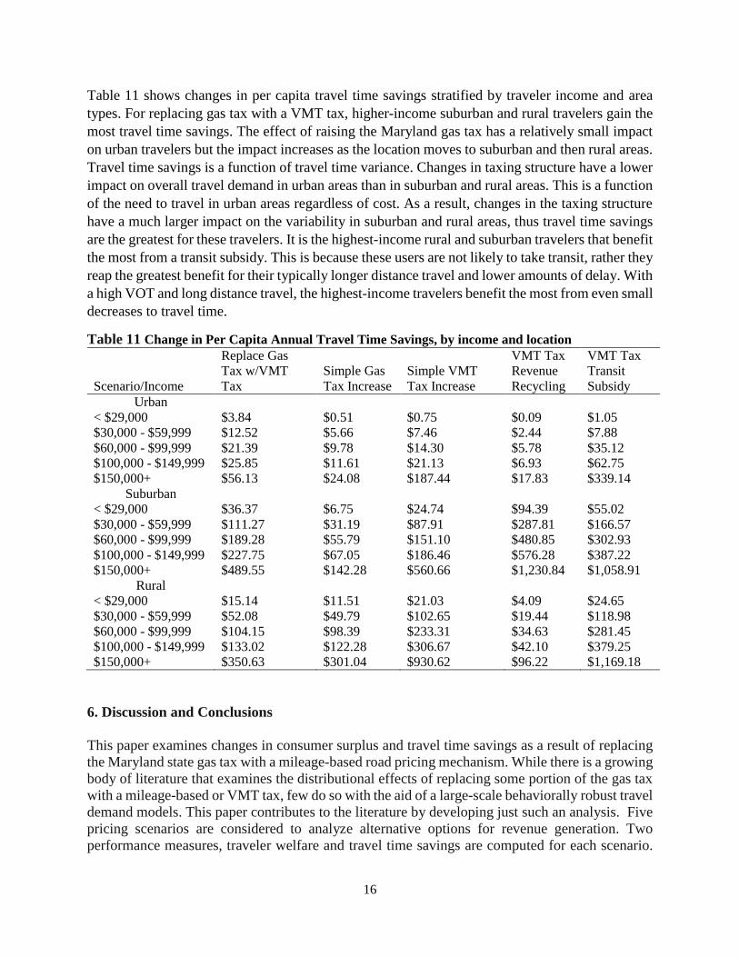
Table 11 shows changes in per capita travel time savings stratified by traveler income and area

types. For replacing gas tax with a VMT tax, higher-income suburban and rural travelers gain the

most travel time savings. The effect of raising the Maryland gas tax has a relatively small impact

on urban travelers but the impact increases as the location moves to suburban and then rural areas.

Travel time savings is a function of travel time variance. Changes in taxing structure have a lower

impact on overall travel demand in urban areas than in suburban and rural areas. This is a function

of the need to travel in urban areas regardless of cost. As a result, changes in the taxing structure

have a much larger impact on the variability in suburban and rural areas, thus travel time savings

are the greatest for these travelers. It is the highest-income rural and suburban travelers that benefit

the most from a transit subsidy. This is because these users are not likely to take transit, rather they

reap the greatest benefit for their typically longer distance travel and lower amounts of delay. With

a high VOT and long distance travel, the highest-income travelers benefit the most from even small

decreases to travel time.

Table 11 Change in Per Capita Annual Travel Time Savings, by income and location

Scenario/Income

Replace Gas

Tax w/VMT

Tax

Simple Gas

Tax Increase

Simple VMT

Tax Increase

VMT Tax

Revenue

Recycling

VMT Tax

Transit

Subsidy

Urban < $29,000 $3.84 $0.51 $0.75 $0.09 $1.05

$30,000 - $59,999 $12.52 $5.66 $7.46 $2.44 $7.88

$60,000 - $99,999 $21.39 $9.78 $14.30 $5.78 $35.12

$100,000 - $149,999 $25.85 $11.61 $21.13 $6.93 $62.75

$150,000+ $56.13 $24.08 $187.44 $17.83 $339.14

Suburban < $29,000 $36.37 $6.75 $24.74 $94.39 $55.02

$30,000 - $59,999 $111.27 $31.19 $87.91 $287.81 $166.57

$60,000 - $99,999 $189.28 $55.79 $151.10 $480.85 $302.93

$100,000 - $149,999 $227.75 $67.05 $186.46 $576.28 $387.22

$150,000+ $489.55 $142.28 $560.66 $1,230.84 $1,058.91

Rural < $29,000 $15.14 $11.51 $21.03 $4.09 $24.65

$30,000 - $59,999 $52.08 $49.79 $102.65 $19.44 $118.98

$60,000 - $99,999 $104.15 $98.39 $233.31 $34.63 $281.45

$100,000 - $149,999 $133.02 $122.28 $306.67 $42.10 $379.25

$150,000+ $350.63 $301.04 $930.62 $96.22 $1,169.18

6. Discussion and Conclusions

This paper examines changes in consumer surplus and travel time savings as a result of replacing

the Maryland state gas tax with a mileage-based road pricing mechanism. While there is a growing

body of literature that examines the distributional effects of replacing some portion of the gas tax

with a mileage-based or VMT tax, few do so with the aid of a large-scale behaviorally robust travel

demand models. This paper contributes to the literature by developing just such an analysis. Five

pricing scenarios are considered to analyze alternative options for revenue generation. Two

performance measures, traveler welfare and travel time savings are computed for each scenario.

17

Results are analyzed by five income groups of travelers and three area types (urban, suburban, and

rural). The complete model set was applied in the state of Maryland using an advanced travel

demand model.

In addition to the base case, five scenarios are developed including: (1) Replace Gas Tax with a

VMT tax, (2) Simple Gas Tax Increase, (3) Simple VMT Tax Increase, (4) VMT Tax Revenue

Recycling, and (5) VMT Tax Transit Subsidy. When each scenario was compared to the Base Case

it was found that all of the changes have a proportionately smaller impact on annual per capita

consumer surplus, compared to the value of travel time savings. Replacing the state gas tax with a

VMT tax can have a positive impact on traveler welfare, particularly for lower-income groups and

rural residents. Increasing either the gas tax or VMT tax will result in mixed effects for different

income groups. Likely, a VMT tax increase would be the least detrimental to welfare, especially

for low-income groups.

The proposed pricing scenarios can be beneficial to identify potential revenue generation sources.

Using revenue obtained from a VMT tax to reduce the federal retail gas tax burden has a significant

impact (relative to the other scenarios) but subsidizing transit fares appears to be the only use that

positively benefits all travelers. Using the revenue from a VMT tax can significantly benefit all

drivers, but has different magnitudes of effect for income and location depending on the use (Burris

et al. 2013). The best use may be a mix of revenue recycling and transit fare subsidy; not quite to

the extremes simulated in this paper. Perhaps the best option in terms of traveler welfare and travel

time savings, if revenue re-use is not an option, is to simply replace the state gas tax with a revenue

neutral VMT tax. The option provides a significant welfare improvement for income groups below

$100,000 and a strong travel time savings benefit for higher-income groups.

This paper provides several advantages for application and practice. First, it provides new insight

for development of prudent strategies to replace the existing state gas tax. Second, a procedural

application of five scenarios is offered that incorporates decision maker’s strategies to examine

travelers’ response. Third, an application of the proposed methodology in a real world multimodal

transportation network that compares model results and quantifies the benefits of each model.

Fourth, the estimation of performance measures such as traveler welfare, travel time savings, VMT

and VHT for each scenario stratified by income groups and area types. Results from each model

provide an array of decision-making options as strategies for replacing the current gas tax and

exploring options from viewpoint of travelers. In this paper, a trip-based model is used to obtain

effects of alternate pricing strategies while each individual characteristic is aggregated to zonal

levels. To obtain each individual’s trip making behavior and elasticity to such policy changes a

micro-level land use and tour-based travel demand model options can be explored in the future

along with more localized network measures such a changes in individual mode preference,

traveler utility and travel time reliability.

18

Appendix

Base Case

A user equilibrium assignment is employed to model user behavior for the base case. The

objective of the model was to simulate each origin-destination (O-D) demand pair till the travel-

cost/travel-time on all used routes of the road network becomes equal (Sheffi 1984). The travel

time function ta(.) is specific to a given link ‘a’ and the most widely used model is the Bureau of

Public Roads (BPR) function given by

𝑡𝑎(𝑥𝑎) = 𝑡𝑜 (1 + 𝛼𝑎 (𝑥𝑎

𝐶𝑎))

𝛽𝑎

(1)

where to(.) is free flow time on link ‘a’, and 𝛼𝑎 and 𝛽𝑎 are constants (and vary by facility type).

𝐶𝑎 is the capacity for link a. In the base model the objective is minimization of total system travel

time. Emission is not a component of the base case.

All Other Scenarios

Pricing for all other scenarios is incorporated into the travel cost function. The revised cost function

becomes as follows:

𝑢𝑎𝐼 (𝑥𝑎, 𝜎) = 𝑡𝑎(𝑥𝑎) +

𝜎𝑙𝑎

𝛾𝑐𝜗 (2)

where, 𝜎 is the gas price in dollars per mile (as a ratio of dollars per gallon), 𝑙𝑎is the link length in

miles, 𝛾𝑐 is the VOT in $/hr, and 𝜗 is the automobile gasoline efficiency in miles per gallon. Auto

Operating Cost (AOC) is another component, which is considered in the mode and destination

choice sections of the model. For brevity details of the destination choice and mode choice are not

presented in this paper, but can be found in Mishra et al. (2012). A higher gas price will result in

a higher AOC and therefore will make auto travel more expensive.

Analytically, the user cost function can be stated as the following to incorporate the VMT-based

tax.

𝑢𝑎𝐼𝐼(𝑥𝑎, 𝑒𝑎, ) = 𝑡𝑎(𝑥𝑎) +

𝜃𝑎𝑙𝑎

𝛾𝑐 (3)

where, 𝜃𝑎 is the VMT tax in $/mile for link a, 𝑙𝑎is the link length in miles, and 𝛾𝑐 is the VOT in

$/hour. In traffic assignment procedure, the user cost shown in equation (7) can be used in equation

(1).

Welfare

We estimate consumer surplus using the rule of half which is an approximation adapted for matrix-

based travel models of the Marshallian consumer surplus (Geurs, 2006).

19

𝐶𝑆𝑖𝑗𝑟 ≅ .5(𝑂𝑖𝑗

𝑏,𝑟𝑓𝑖𝑗𝑏,𝑟 + 𝑂𝑖𝑗

𝑟 𝑓𝑖𝑗𝑟)(𝑡𝑖𝑗

𝑏 (𝑥𝑖𝑗𝑏 ) − 𝑡𝑖𝑗(𝑥𝑖𝑗)) (4)

where O is the vehicle occupancy (in this case either 1, 2 or 3) of vehicles traveling between origin

and destination i-j, f is the traffic flow between origin and destination i-j and the 𝑡𝑖𝑗(𝑥𝑖𝑗) is the

generalized travel cost between zone pairs on the least cost path after highway assignment. This

formulation of traveler welfare assumes a linear demand curve (Geurs, 2006).

Travel Time Variability

The monetized value of travel time savings is estimated as follows.

𝑇𝑇𝑆 = ∑ 𝑣𝑖𝑗 = ∑ ([(∑ 𝑡𝑟𝑎

𝑐 − 𝑡𝑟𝑎

𝑐̅̅̅̅ )2

𝑛 − 1] × (1 + 𝛼𝑎 (𝑦 +

𝑥𝑎

𝐶𝑎))

𝛽𝑎

) (5)

where TTS is the overall travel time savings measure, vij is the variance in congested travel time of

all paths between all origins and destinations, tcra is the congested travel time on the links (a) that

form a given path, 𝑡𝑟𝑎

𝑐̅̅̅̅ is the mean contested travel time between the base and new scenario an n is

the number of links along the given path. The first function is the congested travel time variance.

The parameters 𝛼𝑎 y and 𝛽𝑎 are a modified version of the BPR function.

20

References

Chakraborty, A., and Mishra, S. 2013. Land Use and Transit Ridership Connections: Implications

for State-level Planning Agencies. Land Use Policy, 30(1), pp. 458-469.

Abou-Zeid, M., Ben-Akiva, M., Tierney, K., Buckeye, K., & Buxbaum, J. (2008). Minnesota

Pay-as-You-Drive Pricing Experiment. Transportation Research Record: Journal of the

Transportation Research Board, 2079(-1), 8–14. doi:10.3141/2079-02

Arnott, R., Palma, A. de, & Lindsey, R. (1994). The Welfare Effects of Congestion Tolls with

Heterogeneous Commuters. Journal of Transport Economics and Policy, 28(2), 139–161.

doi:10.2307/20053032

Balducci, P. (2011). Costs of Alternative Revenue-generation Systems (Vol. 689). Transportation

Research Board. Retrieved from

http://books.google.com/books?hl=en&lr=&id=ruSQSByFK1cC&oi=fnd&pg=PP1&dq=

Costs+of+Alternative+Revenue-

Generation+Systems&ots=vb2DEaPD0O&sig=wP0zbN_4aqQ9aBKeeU24hi7xUCI

Bertini, R. L., & Rufolo, A. M. (2004). Technology considerations for the implementation of a

statewide road user fee system. Economic Impacts of Intelligent Transportation Systems:

Innovations and Case Studies. Research in Transportation Economics, 8, 337–361.

Bordoff, J. E., & Noel, P. J. (2008). The impact of pay-as-you-drive auto insurance in california.

Brookings Institution. Retrieved from

http://www.brookings.edu/~/media/Research/Files/Papers/2008/7/payd%20california%20

bordoffnoel/07_payd_california_bordoffnoel.pdf

Burris, M., Lee, S., Geiselbrecht, T., & Baker, R. (2013). Equity Evaluation of Sustainable

Mileage-Based User Fee Scenarios (Technical Report No. SWUTC/14/600451-00007-1).

Southwest Region University Transportation Center. Retrieved from

21

http://d2dtl5nnlpfr0r.cloudfront.net/swutc.tamu.edu/publications/technicalreports/600451

-00007-1.pdf

Button, K. (1995). Road pricing as an instrument in traffic management. In Road Pricing:

Theory, Empirical Assessment and Policy (pp. 35–55). Springer. Retrieved from

http://link.springer.com/chapter/10.1007/978-94-011-0980-2_3

Cervero, R., & Hansen, M. (2002). Induced travel demand and induced road investment: a

simultaneous equation analysis. Journal of Transport Economics and Policy, 469–490.

Ecola, L., & Light, T. (2009). Equity and Congestion Pricing. Rand Corporation, 1–45.

EIA, E. I. A. (2011). Methodologies for estimating fuel consumption using the 2009 national

household travel survey. Federal Highway Administration. Retrieved from

http://nhts.ornl.gov/2009/pub/EIA.pdf

Eliasson, J., & Mattsson, L.-G. (2006). Equity effects of congestion pricing: Quantitative

methodology and a case study for Stockholm. Transportation Research Part A: Policy

and Practice, 40(7), 602–620. doi:10.1016/j.tra.2005.11.002

Felder, S., & van Nieuwkoop, R. (1996). Revenue recycling of a CO2 tax: Results from a general

equilibrium model for Switzerland. Annals of Operations Research, 68(2), 233–265.

Forkenbrock, D. J. (2005). Implementing a mileage-based road user charge. Public Works

Management & Policy, 10(2), 87–100.

Franklin, J. P. (2007). Decomposing the distributional effects of roadway tolls. In Transportation

Research Board 86th Annual Meeting. Retrieved from

http://trid.trb.org/view.aspx?id=802511

22

Fridstrøm, L., Minken, H., Moilanen, P., Shepherd, S., & Vold, A. (2000). Economic and equity

effects of marginal cost pricing in transport. AFFORD Deliverable A, 2. Retrieved from

http://vplno1.vkw.tu-dresden.de/psycho/projekte/afford/download/AFFORDdel2a.pdf

Fuetsch, M. (2009). National VMT tax system could use current technology, Minn. study says.

Transport Topics, (3862). Retrieved from http://trid.trb.org/view.aspx?id=901753

Geurs, K. (2006). Accessibility, land use and transport. Eburon Uitgeverij B.V.

Glaister, S., & Graham, D. J. (2005). An evaluation of national road user charging in England.

Transportation Research Part A: Policy and Practice, 39(7), 632–650.

Greene, D. L. (2011). What is greener than a VMT tax? The case for an indexed energy user fee

to finance us surface transportation. Transportation Research Part D: Transport and

Environment, 16(6).

Kim, D. S., Porter, D., & Wurl, R. (2002). Technology Evaluation for Implementation of VMT

Based Revenue Collection Systems. Salem, OR: Oregon Department of Transportation.

Report No. FHWA-OR-VP-03-07. Retrieved from

http://www.oblpct.state.or.us/ODOT/HWY/OIPP/docs/OSU_VMT_Final_Report_WEB.

pdf

Kim, D. S., Porter, J. D., Whitty, J., Svadlenak, J., Larsen, N. C., Capps, D. F., … Hall, D. D.

(2008). Technology evaluation of Oregon’s vehicle-miles-traveled revenue collection

system: Lessons learned. Transportation Research Record: Journal of the Transportation

Research Board, 2079(1), 37–44.

Kockelman, K., Fagnant, D., Nichols, B., & Boyles, S. (2012). A Project Evaluation Toolkit

(PET) for Abstracted Networks. Retrieved from http://trid.trb.org/view.aspx?id=1243218

23

Levinson, D. (2010). Equity Effects of Road Pricing: A Review. Transport Reviews, 30(1), 33–

57. doi:10.1080/01441640903189304

Margiotta, R., Lomax, T., Hallenbeck, M., Dowling, R., Skabardonis, A., & Turner, S. (2013).

Analytical Procedures for Determining the Impacts of Reliability Mitigation Strategies.

SHRP 2 Report, (S2-L03-RR-1). Retrieved from

http://pubsindex.trb.org/view/2013/M/1226380

May, A. D., & Milne, D. S. (2000). Effects of alternative road pricing systems on network

performance. Transportation Research Part A: Policy and Practice, 34(6), 407–436.

Md. gas tax: The cost of doing nothing. (n.d.). Baltimore Sun. Retrieved March 21, 2013, from

http://articles.baltimoresun.com/2011-03-10/news/bs-ed-gas-tax-20110310_1_gas-tax-

price-spike-gasoline-prices

NTD. (2011). National Transit Database: TS 2 Operating Expenses, Service Supplied and

Consumed Dataset (No. TS2). Washington DC. Retrieved from

http://www.ntdprogram.gov/ntdprogram/data.htm

NYSDOT Task Assignment, C. (2012). Mileage-Based User Fees: Prospects and Challenges.

Retrieved from

http://citeseerx.ist.psu.edu/viewdoc/download?doi=10.1.1.258.8533&rep=rep1&type=pdf

Parry, I. W. (2005). Is Pay-as-You-Drive insurance a better way to reduce gasoline than gasoline

taxes? American Economic Review, 288–293.

Parry, I. W. H., & Bento, A. (2001). Revenue Recycling and the Welfare Effects of Road

Pricing. Scandinavian Journal of Economics, 103(4), 645–671. doi:10.1111/1467-

9442.00264

24

Parry, I. W. H., & Small, K. A. (2005). Does Britain or the United States Have the Right

Gasoline Tax? The American Economic Review, 95(4), 1276–1289.

doi:10.1257/0002828054825510

Peters, J. R., & Kramer, J. K. (2012). Just Who Should Pay for What? Vertical Equity, Transit

Subsidy and Road Pricing: The Case of New York City. Journal of Public

Transportation, 15(2), 117–136.

Santos, G., & Rojey, L. (2004). Distributional impacts of road pricing: The truth behind the

myth. Transportation, 31(1), 21–42.

Shackleton, R., Shelby, M., Cristofaro, A., Brinner, R., Yanchar, J., Goulder, L., … Kaufman, R.

(1992). The efficiency value of carbon tax revenues. US Environmental Protection

Agency Washington DC. Retrieved from

http://emf.stanford.edu/files/pubs/22440/WP1208.pdf

Smalkoski, B., & Levinson, D. (2005). Value of time for commercial vehicle operators in

Minnesota. In Journal of the Transportation Research Forum (Vol. 44, pp. 89–102).

Small, K. A. (1992). Using the revenues from congestion pricing. Transportation, 19(4), 359–

381. doi:10.1007/BF01098639

Sorensen, P. A., & Taylor, B. D. (2005). Review and synthesis of road-use metering and

charging systems. Transportation Research Board. Retrieved from

http://its.ucla.edu/research/rpubs/Sorensen_Taylor_v8.pdf

Starr McMullen, B., Zhang, L., & Nakahara, K. (2010). Distributional impacts of changing from

a gasoline tax to a vehicle-mile tax for light vehicles: A case study of Oregon. Transport

Policy, 17(6), 359–366. doi:10.1016/j.tranpol.2010.04.002

25

Strand, J. (1998). Pollution taxation and revenue recycling under monopoly unions. The

Scandinavian Journal of Economics, 100(4), 765–780.

Verhoef, E. T. (2002). Second-best congestion pricing in general networks. Heuristic algorithms

for finding second-best optimal toll levels and toll points. Transportation Research Part

B: Methodological, 36(8), 707–729.

Weatherford, B. (2011). Distributional Implications of Replacing the Federal Fuel Tax with Per

Mile User Charges. Transportation Research Record: Journal of the Transportation

Research Board, 2221(-1), 19–26. doi:10.3141/2221-03

Welch, T. F., & Mishra, S. (Forthcoming). Envisioning an emission diet: application of travel

demand mechanisms to facilitate policy decision making. Transportation, 1–21.

doi:10.1007/s11116-013-9511-4

Zhang, L., & McMullen, B. S. (2008). Statewide distance-based user charge: Case of Oregon. In

Transportation Research Board 87th Annual Meeting. Retrieved from

http://trid.trb.org/view.aspx?id=848406

Zhang, L., McMullen, B. S., Valluri, D., & Nakahara, K. (2009). The short-and long-run impact

of a vehicle mileage fee on income and spatial equity. Transportation Research Record:

Journal of the Transportation Research Board, 2115, 110–118.