distribution network supports for transmission system
TRANSCRIPT

DISTRIBUTION NETWORK SUPPORTS FOR
TRANSMISSION SYSTEM REACTIVE
POWER MANAGEMENT
A thesis submitted to The University of Manchester for the degree of
Doctor of Philosophy
in the Faculty of Engineering and Physical Sciences
2015
LINWEI CHEN
SCHOOL OF ELECTRICAL AND ELECTRONIC ENGINEERING

2
LIST OF CONTENTS
LIST OF CONTENTS ...................................................................................................... 2
LIST OF FIGURES ........................................................................................................... 7
LIST OF TABLES ........................................................................................................... 11
LIST OF ABBREVIATIONS AND SYMBOLS ........................................................... 12
LIST OF PUBLICATIONS ............................................................................................ 16
ABSTRACT ..................................................................................................................... 17
DECLARATION ............................................................................................................. 18
COPYRIGHT STATEMENT ........................................................................................ 19
ACKNOWLEDGEMENTS ............................................................................................ 20
1 INTRODUCTION .................................................................................................... 21
1.1 Low Carbon Electricity Networks ...................................................................... 21
1.2 Voltage and Reactive Power Control .................................................................. 24
1.3 Motivation ........................................................................................................... 26
1.4 Research Objectives ............................................................................................ 29
1.5 List of Main Contributions to Work ................................................................... 30
1.6 Thesis Outline ..................................................................................................... 31
2 LITERATURE REVIEW ........................................................................................ 34
2.1 Introduction ......................................................................................................... 34
2.2 Traditional Voltage Regulation Methods ........................................................... 34
2.2.1 Transmission system voltage control .......................................................... 35
2.2.2 Distribution system voltage control ............................................................. 39
2.3 Voltage Control Methods with Distributed Generation ...................................... 44
2.3.1 On-load tap changer control ........................................................................ 44

3
2.3.2 Reactive power control ................................................................................ 47
2.3.3 Power curtailment ........................................................................................ 49
2.4 Reactive Power Management in Transmission Systems .................................... 50
2.4.1 Generation and absorption of reactive power .............................................. 51
2.4.2 Reactive power ancillary service ................................................................. 53
2.4.3 Reactive power dispatch .............................................................................. 55
2.4.4 Distribution network VAr support for transmission system........................ 55
2.5 Volt/VAr Optimisation Control .......................................................................... 57
2.5.1 Problem description ..................................................................................... 57
2.5.2 Solution algorithms ..................................................................................... 58
2.6 Summary ............................................................................................................. 61
3 FUNDAMENTALS OF DISTRIBUTION SYSTEMS ......................................... 63
3.1 Introduction ......................................................................................................... 63
3.2 Distribution System Structure ............................................................................. 63
3.3 Voltage Regulation ............................................................................................. 65
3.3.1 Voltage drop calculations ............................................................................ 65
3.3.2 Allowable voltage variations ....................................................................... 66
3.4 Transformer with On-load Tap Changer ............................................................ 67
3.4.1 Tap changer mechanisms ............................................................................ 67
3.4.2 Per-unit model of transformer with tap changer .......................................... 69
3.5 Summary ............................................................................................................. 71
4 TAP STAGGER FOR REACTIVE POWER SUPPORT .................................... 73
4.1 Introduction ......................................................................................................... 73
4.2 Proposed Distribution Network VAr Support Method with Tap Stagger .......... 73
4.3 Tap Stagger Mathematic Principles .................................................................... 75
4
4.3.1 Parallel operation of two transformers ........................................................ 75
4.3.2 Equivalent circuit for tap stagger ................................................................ 77
4.4 Tap Stagger Optimal Control .............................................................................. 83
4.4.1 Objective function ....................................................................................... 84
4.4.2 Constraints ................................................................................................... 85
4.5 Summary ............................................................................................................. 86
5 NETWORK REACTIVE POWER ABSORPTION CAPABILITY STUDIES . 88
5.1 Introduction ......................................................................................................... 88
5.2 Distribution Network Modelling ........................................................................ 88
5.3 Maximum VAr Absorption Capability Studies .................................................. 89
5.3.1 Case 1: Reactive power absorption capability of single pair of parallel
transformers ............................................................................................................... 90
5.3.2 Case 2: Aggregated reactive power absorption of twenty pairs of parallel
transformers ............................................................................................................... 94
5.4 Conservative VAr Absorption Capability Studies .............................................. 97
5.5 Summary ............................................................................................................. 99
6 IMPLEMENTATION OF TAP STAGGER CONTROL USING GA .............. 101
6.1 Introduction ....................................................................................................... 101
6.2 Network Modelling in OpenDSS ...................................................................... 101
6.2.1 Network transfer from IPSA to OpenDSS ................................................ 102
6.2.2 Validation of OpenDSS network model .................................................... 106
6.3 Tap Stagger Control based on Genetic Algorithm ............................................ 108
6.3.1 Control variable encoding ......................................................................... 109
6.3.2 Fitness function ......................................................................................... 109
6.3.3 Genetic operators ....................................................................................... 110
6.3.4 Computational procedure .......................................................................... 112
5
6.4 Testing of GA-based Control ............................................................................ 113
6.4.1 Parameter assignment ................................................................................ 113
6.4.2 Optimisation results ................................................................................... 114
6.5 Effects of Different Load Models ..................................................................... 118
6.6 Time-Series Studies with Daily Load Profile ................................................... 120
6.7 Summary ........................................................................................................... 124
7 COMPARISON OF GA WITH OTHER SOLUTION METHODS ................. 126
7.1 Introduction ....................................................................................................... 126
7.2 Alternative Control Methods for Tap Stagger .................................................. 126
7.2.1 Rule-based control scheme ........................................................................ 127
7.2.2 Branch-and-bound solution method .......................................................... 129
7.3 Comparison Studies for 102-Bus Distribution Network................................... 132
7.3.1 Case 1: Convergence analysis with different VAr requirements .............. 133
7.3.2 Case 2: Sensitivity analysis with different settings of reactive power
absorption accuracy ................................................................................................. 138
7.3.3 Case 3: Sensitivity analysis with different settings of maximum staggered
taps…… ................................................................................................................... 141
7.3.4 Summary of findings ................................................................................. 144
7.4 Comparison Studies for 222-Bus Distribution Network................................... 145
7.4.1 Case 1: Convergence and computation time analyses with different VAr
requirements ............................................................................................................ 146
7.4.2 Case 2: Comparison of time-series optimisation studies ........................... 149
7.4.3 Summary of findings ................................................................................. 153
7.5 Summary ........................................................................................................... 153
8 IMPACTS OF TAP STAGGER ON TRANSMISSION SYSTEM ................... 155
8.1 Introduction ....................................................................................................... 155
6
8.2 Transmission System Modelling and Tap Stagger Implementation ................. 155
8.2.1 IEEE reliability test system ....................................................................... 155
8.2.2 Identification of voltage problems ............................................................. 157
8.2.3 Implementation of tap stagger using GA ................................................... 159
8.2.4 Cost Analysis for VAr Compensation ....................................................... 161
8.3 Effectiveness on Voltage Regulation ................................................................ 162
8.4 Economic Studies ............................................................................................. 164
8.4.1 Case 1: Cost analysis for bus with occasional voltage issues ................... 164
8.4.2 Case 2: Cost analysis for bus with frequent voltage issues ....................... 166
8.4.3 Case 3: Combined method of reactor and tap Stagger .............................. 167
8.5 Dynamic Performance Studies .......................................................................... 169
8.5.1 Reactor switching in transmission network ............................................... 170
8.5.2 Tap staggering in distribution network ...................................................... 171
8.6 Summary ........................................................................................................... 174
9 CONCLUSIONS .................................................................................................... 176
9.1 Conclusions ....................................................................................................... 176
9.2 Suggestions for Future Work ............................................................................ 181
REFERENCES .............................................................................................................. 184
APPENDIX A ................................................................................................................. 194
APPENDIX B ................................................................................................................. 196
APPENDIX C ................................................................................................................. 198
APPENDIX D ................................................................................................................. 203
APPENDIX E ................................................................................................................. 209
Final word count: 48366
7
LIST OF FIGURES
Figure 1-1: Electricity generation by main renewable sources since 2000 [6] ................. 22
Figure 1-2: Modern electric power system with distributed generation ............................ 23
Figure 1-3: Voltage and reactive power control with different components and devices in
power system ..................................................................................................................... 25
Figure 1-4: Minimum national active (GW) and reactive (GVAr) power demands
(average of 3 lowest each year) [26] ................................................................................. 28
Figure 2-1: Block diagram of a closed-loop automatic voltage regulator [37] ................. 35
Figure 2-2: General principle of the secondary voltage control loop [41] ........................ 37
Figure 2-3: Basic arrangement of an OLTC transformer with AVC relay [21] ................ 40
Figure 2-4: Key elements of the line-drop compensation [21] .......................................... 41
Figure 2-5: Phasor diagram for the LDC method .............................................................. 42
Figure 2-6: Schematic of a step voltage regulator [18] ..................................................... 43
Figure 2-7: Voltage profile of a feeder with a voltage regulator (R1), supplementary
regulator (R2) and a shunt capacitor bank (C) [18] ............................................................ 43
Figure 2-8: SuperTAPP n+ relay arrangement [58] .......................................................... 45
Figure 2-9: Single-line model of distribution network with distributed generator [67] .... 48
Figure 2-10: Low voltage feeder with PVs [73] ................................................................ 50
Figure 2-11: Examples of SVC and STATCOM topologies [18], [79] ............................ 53
Figure 2-12: Single-line diagrams of radial transmission line feeding M load centres with
the voltage support provided on (a) transmission buses, and (b) distribution buses [103] 56
Figure 3-1: General arrangement of a distribution system with different voltage levels [36]
........................................................................................................................................... 64
Figure 3-2: Single-phase equivalent circuit of a line segment in distribution system ....... 66
Figure 3-3: Principle winding arrangement of a regulating transformer in Y-∆ connection
[117] .................................................................................................................................. 67
Figure 3-4: Loss of system load with single contact switching [117] ............................... 68
Figure 3-5: Switching sequence of an OLTC with tap selector-diverter switch [117] ..... 69
Figure 3-6: Single-line diagram of transformer (a) with off-nominal turns ratio, and (b)
represented as two transformers in series [119] ................................................................ 70
8
Figure 3-7: Models of transformer with off-nominal turns ratio: (a) per-unit equivalent
circuit, and (b) π circuit representation [119] .................................................................... 71
Figure 4-1: Proposed reactive power absorption service provided by distribution network
using tap stagger ................................................................................................................ 74
Figure 4-2: Single-line diagram of two parallel transformers ........................................... 76
Figure 4-3: Schematic of tap stagger ................................................................................. 77
Figure 4-4: Equivalent circuit of tap stagger (referred to the transformer secondary sides)
[121] .................................................................................................................................. 77
Figure 4-5: Phasor diagram of tap staggering on transformer T1 and T2 .......................... 79
Figure 4-6: Transformer secondary voltage with different staggered taps (with ∆TAP =
1.43% and TAP0 = 0.9714 pu) ........................................................................................... 82
Figure 4-7: Block diagram of the tap stagger optimal control .......................................... 86
Figure 5-1: Structure of a real UK distribution system modelled in IPSA ....................... 89
Figure 5-2: Example of two parallel transformers at a primary substation in the IPSA
model ................................................................................................................................. 91
Figure 5-3: Additional reactive power absorption of a pair of parallel transformers with
tap stagger .......................................................................................................................... 93
Figure 5-4: Additional active power losses of a pair of parallel transformers with tap
stagger ................................................................................................................................ 93
Figure 5-5: Aggregated Q absorption from 20 pairs of parallel transformers (with
maximum staggered taps) .................................................................................................. 96
Figure 5-6: Aggregated P losses from 20 pairs of parallel transformers (with maximum
staggered taps) ................................................................................................................... 97
Figure 5-7: Aggregated Q absorption from 20 pairs of parallel transformers (with 4
staggered taps) ................................................................................................................... 98
Figure 5-8: Aggregated P losses from 20 pairs of parallel transformers (with 4 staggered
taps) ................................................................................................................................... 99
Figure 6-1: Screenshot of the simplified distribution network in IPSA .......................... 103
Figure 6-2: Network structure of the modified 102-bus distribution system .................. 104
Figure 6-3: Screenshot of the IPSA modelling script for the modified 102-bus distribution
system .............................................................................................................................. 104

9
Figure 6-4: Screenshot of the OpenDSS modelling scripts for the 102-bus distribution
system .............................................................................................................................. 105
Figure 6-5: The OpenDSS structure [128] ...................................................................... 105
Figure 6-6: Absolute errors between the OpenDSS and IPSA calculated bus voltages .. 107
Figure 6-7: Example of a pair of primary substation transformers with staggered taps (in
IPSA and OpenDSS) ....................................................................................................... 108
Figure 6-8: Mechanism of the stochastic uniform sampling method .............................. 111
Figure 6-9: Flowchart of the GA-based solution procedure ............................................ 112
Figure 6-10: Information about individuals in each generation ...................................... 114
Figure 6-11: Optimisation results with different reactive power requirements (with elimit =
1% & TSmax = 4) .............................................................................................................. 117
Figure 6-12: Reactive power absorption observed at the GSP by using the tap staggering
technique .......................................................................................................................... 120
Figure 6-13: Daily load profile used in the simulations (with half-hourly resolution) ... 121
Figure 6-14: Optimisation results for the 102-bus network with 24-hour study (at Qrequired
= 1.0 MVAr & elimit = 1%) .............................................................................................. 123
Figure 6-15: Reactive power absorption errors of the 24-hour optimisation studies for
different load models ....................................................................................................... 124
Figure 7-1: Flowchart of the rule-based control scheme ................................................. 128
Figure 7-2: Binary search tree [135] ............................................................................... 132
Figure 7-3: Optimisation results with different control methods for the 102-bus
distribution system (with elimit = 1% and TSmax = 4) ........................................................ 136
Figure 7-4: Optimisation results for the 102-bus distribution system using different
settings of elimit (with Qrequired = 0.5 to 2 MVAr & TSmax = 4) ......................................... 140
Figure 7-5: Optimisation results for the 102-bus distribution system using different
settings of TSmax (with Qrequired = 0.5 to 2 MVAr & elimit = 1%) ...................................... 143
Figure 7-6: Optimisation results with different control methods for the 222-bus
distribution system (with elimit = 1% and TSmax = 4) ........................................................ 148
Figure 7-7: Optimisation results for the 222-bus network using 24-hour load profile (at
Qrequired = 3 MVAr & elimit = 1%) .................................................................................... 151

10
Figure 7-8: Reactive power absorption errors of the 24-hour optimisation studies for
different solution methods ............................................................................................... 152
Figure 8-1: Single-line diagram of the IEEE Reliability Test System ............................ 156
Figure 8-2: Annual load profile for the RTS system (in percent of annual peak load) ... 157
Figure 8-3: Annual voltage profile of the RTS system ................................................... 158
Figure 8-4: Flowchart to determine load increments when applying the tap staggering
technique to the RTS system ........................................................................................... 160
Figure 8-5: Total number of annual voltage violations (i.e. > 1.05 pu) with tap stagger
applied at either bus 6 or bus 10 ...................................................................................... 163
Figure 8-6: Annual energy generation for the RTS system with either reactor or tap
stagger .............................................................................................................................. 165
Figure 8-7: Annual costs for solutions 1 and 2 in Case 1 (at compensation level of 6
MVAr) ............................................................................................................................. 166
Figure 8-8: Annual costs for solutions 3 and 4 in Case 1 (at compensation level of 6
MVAr) ............................................................................................................................. 167
Figure 8-9: Modified RTS system for dynamic studies .................................................. 169
Figure 8-10: Bus 6 voltage with 1 MVAr reactor switching on and off at bus 6 ............ 170
Figure 8-11: Buses 2 & 10 voltages with the reactor switching at bus 6 ........................ 171
Figure 8-12: Bus 6 voltage with the application of tap stagger at the five primary
substations ....................................................................................................................... 172
Figure 8-13: Buses 2 & 10 voltages with the application of tap stagger at the five primary
substations ....................................................................................................................... 173
Figure 8-14: Bus voltages with only three pairs of primary transformers tap staggering
......................................................................................................................................... 174
Figure 9-1: Real-time implementation of the tap stagger optimal control ...................... 182
11
LIST OF TABLES
Table 5-1: Reactive power variations of a single pair of primary substation transformers
with tap stagger .................................................................................................................. 92
Table 5-2: Active power variations of a single pair of primary substation transformers
with tap stagger .................................................................................................................. 92
Table 5-3: Additional VAr absorption and power loss of distribution system with tap
staggered transformers ....................................................................................................... 94
Table 6-1: Statistics of bus voltage errors between the OpenDSS and IPSA models ..... 107
Table 6-2: Parameters of the GA optimisation algorithm ............................................... 113
Table 6-3: Optimisation results with GA running ten times for each value of Qrequired (at
elimit = 1% & TSmax = 4) ................................................................................................... 116
Table 6-4: GA optimisation results for different load models used in the distribution
network (elimit = 1% & TSmax = 4) .................................................................................... 119
Table 7-1: Optimisation results for each value of Qrequired using different control
algorithms (at elimit = 1% & TSmax = 4) ............................................................................ 134
Table 7-2: Number of converged solutions for the VAr requirement from 0.1 to 2.5
MVAr .............................................................................................................................. 135
Table 7-3: Tap staggering arrangements of primary substations to provide reactive power
absorption ........................................................................................................................ 135
Table 7-4: Computation time for the 102-bus distribution system studies ..................... 137
Table 7-5: Optimisation results with different settings of elimit (with TSmax = 4) ............ 139
Table 7-6: Optimisation results with different settings of TSmax (with elimit = 1%) ......... 142
Table 7-7: Optimisation results of the 222-bus distribution network for different Qrequired
(with elimit = 1% & TSmax = 4) .......................................................................................... 147
Table 7-8: Computation time for the 222-bus distribution system studies ..................... 149
Table 7-9: 24-hour optimisation results for the 222-bus network with different settings of
Qrequired ............................................................................................................................. 152
Table 8-1: Annual costs for solutions 5, 6 and 7 in case 3 .............................................. 168
Table 8-2: Transient voltage responses with reactor switching ...................................... 171
Table 8-3: Transient voltage responses with transformer tap staggering ........................ 173

12
LIST OF ABBREVIATIONS AND SYMBOLS
Abbreviations
AVC automatic voltage control
AVR automatic voltage regulator
CSVC coordinated secondary voltage control
DG distributed generation
DMS distribution management system
DNO distribution network operator
DP dynamic programming
DSE distribution state estimation
EHV extra high voltage, i.e. 275kV and 400kV
GA genetic algorithm
GSP grid supply point
HV high voltage, i.e. from 33kV to 132kV
LDC line drop compensation
LP linear programming
LV low voltage, i.e. lower than 1kV
MINLP mixed-integer nonlinear programming
MV medium voltage, i.e. from 1kV to 33kV
OLTC on-load tap changer
OPF optimal power flow
PV photovoltaic generator
RTU remote terminal unit
STATCOM static synchronous compensator
SVC static VAr compensator
SVR step voltage regulator
RTS Reliability Test System
TSO transmission system operator
TVC tertiary voltage control
13
Symbols
∆h time interval of applying the tap staggering technique
∆Pc additional active power loss of two parallel transformers due to tap
stagger
∆Ploss active power loss of distribution network caused by tap stagger
∆Pt,n active power loss of distribution network with Qrequired = n MVAr at the
time point t
∆Qc additional reactive power absorption of two parallel transformers due to
tap stagger
∆Qlines additional reactive power consumption of lines due to tap stagger
∆Qloads additional reactive power consumption of loads due to tap stagger
∆Qt,n reactive power absorption measured at GSP with Qrequired = n MVAr at
the time point t
∆𝑄𝑡𝑚 total reactive power absorption (in MVAr) provided through the use of
tap stagger at the time point tm
∆Qtransformers additional reactive power consumption of transformers due to tap stagger
∆TAP tap position increment (%) per tap step of OLTC
Ci,j reactive power absorption that could be individually provided by the ith
pair of parallel transformers with 2j staggered taps (i.e. j taps up for one
and j taps down for the other)
Creactor annual cost for TSO to apply reactors to reduce high voltages
Cstagger annual cost for TSO to apply the tap staggering technique
CVAr unit price of reactive energy in £/MVArh
C∆gen(h) cost to compensate generation changes due to tap stagger
C∆gen’(h) cost to compensate generation changes due to the use of reactors
C network reactive power absorption capability matrix
elimit maximum permitted error (%) between the required and the actual
reactive power absorption provided
h total hours of using tap stagger in a year, i.e. the utilisation hour
I annual equivalent investment cost of installing a reactor
I1 secondary current on Transformer T1
14
I2 secondary current on Transformer T2
Ic circulating current around two parallel transformers
k number of tap steps increased or decreased from the initial tap position
M maximum allowable tap difference from the initial tap position
nm nominal transformer ratio
N total number of pairs of parallel transformers involved in the tap stagger
optimisation
Ne number of elites
Npop population size
Pi,j network loss caused by the ith
pair of parallel transformers with 2j
staggered taps (i.e. j taps up for one and j taps down for the other)
P network power loss matrix due to tap stagger
Qactual actual reactive power absorbed by the downstream distribution network
through the use of tap stagger
Qrequired additional reactive power absorption required by the upstream
transmission network to maintain system voltages
r discount rate
R2 coefficient of determination
S actual capital investment of installing a reactor
T total time points in a year
TAP0 initial transformer tap position in per-unit
TAPi initial tap positions on the ith
pair of parallel transformers in per-unit
TAPi,max upper limit of the tap positions on the ith
pair of parallel transformers
TAPi,min lower limit of the tap positions on the ith
pair of parallel transformers
TSmax maximum allowable difference between the tap positions of two parallel
transformers without causing overheating and damages
V1 primary voltage referred to the secondary side of Transformer T1
V2 primary voltage referred to the secondary side of Transformer T2
Vp transformer primary voltage
Vs transformer secondary voltage (connected to loads)

15
w1 weighting coefficient of active power loss
w2 weighting coefficient of tap changer switching operations
w3 weighting coefficient of reactive power absorption
xi number of tap steps different from the initial tap positions on the ith
pair
of parallel transformers
xi,j binary integer that determines whether to tap apart the ith
pair of parallel
transformers
x tap staggering control vector
y economic life of a reactor
Zt transformer equivalent series impedance in ohms, referred to the
secondary side
Zt,pu transformer equivalent series impedance in per-unit
ZL equivalent load impedance in ohms

16
LIST OF PUBLICATIONS
1) L. Chen, and H. Li, “Optimised reactive power supports using transformer tap stagger
in distribution networks,” IEEE Transactions on Smart Grid, submitted in Sep. 2015.
2) L. Chen, and H. Li, “Ancillary service for transmission systems by tap stagger
operation in distribution networks,” IEEE Transactions on Power Delivery, submitted
in Aug. 2015.
3) L. Chen, H. Li, V. Turnham, and S. Brooke, "Distribution network supports for
reactive power management in transmission systems," IEEE PES Innovative Smart
Grid Technologies (ISGT) European, Istanbul, Oct. 2014.
4) S. Qi, L. Chen, H. Li, D. Randles, G. Bryson, and J. Simpson, “Assessment of voltage
control techniques for low voltage networks,” 12th
International Conference on
Developments in Power System Protection, Copenhagen, Apr. 2014.
5) L. Chen, S. Qi, and H. Li, “Improved adaptive voltage controller for active distribution
network operation with distributed generation,” 47th
International Universities Power
Engineering Conference, London, Sep. 2012.

17
ABSTRACT
The University of Manchester
Linwei Chen
A thesis submitted for the degree of Doctor of Philosophy
Distribution Network Supports for Transmission System Reactive Power Management
November 2015
To mitigate high voltages in transmission systems with low demands, traditional
solutions often consider the installation of reactive power compensators. The deployment
and tuning of numbers of VAr compensators at various locations may not be cost-
effective. This thesis presents an alternative method that utilises existing parallel
transformers in distribution networks to provide reactive power supports for transmission
systems under low demands. The operation of parallel transformers in small different tap
positions, i.e. with staggered taps, can provide a means of absorbing reactive power. The
aggregated reactive power absorption from many pairs of parallel transformers could be
sufficient to provide voltage support to the upstream transmission network.
Network capability studies have been carried out to investigate the reactive power
absorption capability through the use of tap stagger. The studies are based on a real UK
High Voltage distribution network, and the tap staggering technique has been applied to
primary substation transformers. The results confirm that the tap staggering method has
the potential to increase the reactive power demand drawn from the transmission grid.
This thesis also presents an optimal control method for tap stagger to minimise the
introduced network loss as well as the number of tap switching operations involved. A
genetic algorithm (GA) based procedure has been developed to solve the optimisation
problem. The GA method has been compared with two alternative solution approaches,
i.e. the rule-based control scheme and the branch-and-bound algorithm. The results
indicate that the GA method is superior to the other two approaches.
The economic and technical impacts of the tap staggering technique on the transmission
system has been studied. In the economic analysis, the associated costs of applying the
tap staggering method have been investigated from the perspective of transmission
system operator. The IEEE Reliability Test System has been used to carry out the studies,
and the results have been compared with the installation of shunt reactors. In the technical
studies, the dynamic impacts of tap staggering or reactor switching on transmission
system voltages have been analysed. From the results, the tap staggering technique has
more economic advantages than reactors and can reduce voltage damping as well as
overshoots during the transient states.

18
DECLARATION
No portion of the work referred to in this thesis has been submitted in support of an
application for another degree of qualification of this or any other university or other
institution of learning.

19
COPYRIGHT STATEMENT
i. The author of this thesis (including any appendices and/or schedules to this thesis)
owns certain copyright or related rights in it (the “Copyright”) and he has given The
University of Manchester certain rights to use such Copyright, including for
administrative purposes.
ii. Copies of this thesis, either in full or in extracts and whether in hard or electronic
copy, may be made only in accordance with the Copyright, Designs and Patents Act
1988 (as amended) and regulations issued under it or, where appropriate, in
accordance with licensing agreements which the University has from time to time.
This page must form part of any such copies made.
iii. The ownership of certain Copyright, patents, designs, trade marks and other
intellectual property (the “Intellectual Property”) and any reproductions of copyright
works in the thesis, for example graphs and tables (“Reproductions”), which may be
described in this thesis, may not be owned by the author and may be owned by third
parties. Such Intellectual Property and Reproductions cannot and must not be made
available for use without the prior written permission of the owner(s) of the relevant
Intellectual Property and/or Reproductions.
iv. Further information on the conditions under which disclosure, publication and
commercialisation of this thesis, the Copyright and any Intellectual Property and/or
Reproductions described in it may take place is available in the University IP Policy
(see http://documents.manchester.ac.uk/DocuInfo.aspx?DocID=487), in any relevant
Thesis restriction declarations deposited in the University Library, The University
Library’s regulations (see http://www.manchester.ac.uk/library/aboutus/regulations)
and in The University’s policy on Presentation of Theses.

20
ACKNOWLEDGEMENTS
I would like to express my heartfelt gratitude to all those who gave me the possibility to
complete this project.
My deepest gratitude goes first and foremost to Dr Haiyu Li, my supervisor, for his
constant encouragement and guidance. Without his consistent and illuminating
instruction, this project could not have reached its present form.
I would like to thank the Your Manchester Fund and the School of Electrical and
Electronic Engineering for providing the financial support for my PhD.
I would also like to express my appreciation to my wife, Yiren Wang, who gives me her
never ending support and encouragement through my life.
Especially, my thanks would go to my beloved parents for their unconditional love and
great confidence in me all through these years.

CHAPTER 1 INTRODUCTION
School of Electrical and Electronic Engineering 21
CHAPTER 1
1 INTRODUCTION
1.1 Low Carbon Electricity Networks
Climate change, which includes global warming, sea level rise and extreme weather, has
been drawing more and more public concern over the years. There is compelling
evidence that the major cause of climate change is human activities, for instance burning
fossil fuels, transport and industrial processes [1], [2]. The carbon emissions from such
activities have exacerbated the greenhouse effect, which has resulted in the observed
temperature increases. Concerning the increasing greenhouse gas (GHG) emission issues,
the European Council has published the “20 20 by 2020” package, which aims to reduce
at least 20% of GHG emissions and to increase the share of renewable energy
consumption in the European Union (EU) to 20% [3]. In the United Kingdom (UK), the
‘Climate Change Act of 2008’ also specifies the government’s duty to reduce the net UK
carbon account for the year 2050 at least 80% lower than 1990 [4].
In 2013, the UK domestic GHG emissions were 564 MtCO2e (i.e. metric tonne carbon
dioxide equivalent), with 26% coming from the electric power sector [5]. As the
electricity generation produces the largest portion of emissions, decarbonising the power
sector is the key part of carbon reduction. The renewable energy generation with few
GHG emissions is therefore considered as one of the most effective ways to construct low
carbon networks. According to the National Renewable Statistics, the UK electricity
generated from renewable sources increased by 113% between 2009 and 2013, to reach
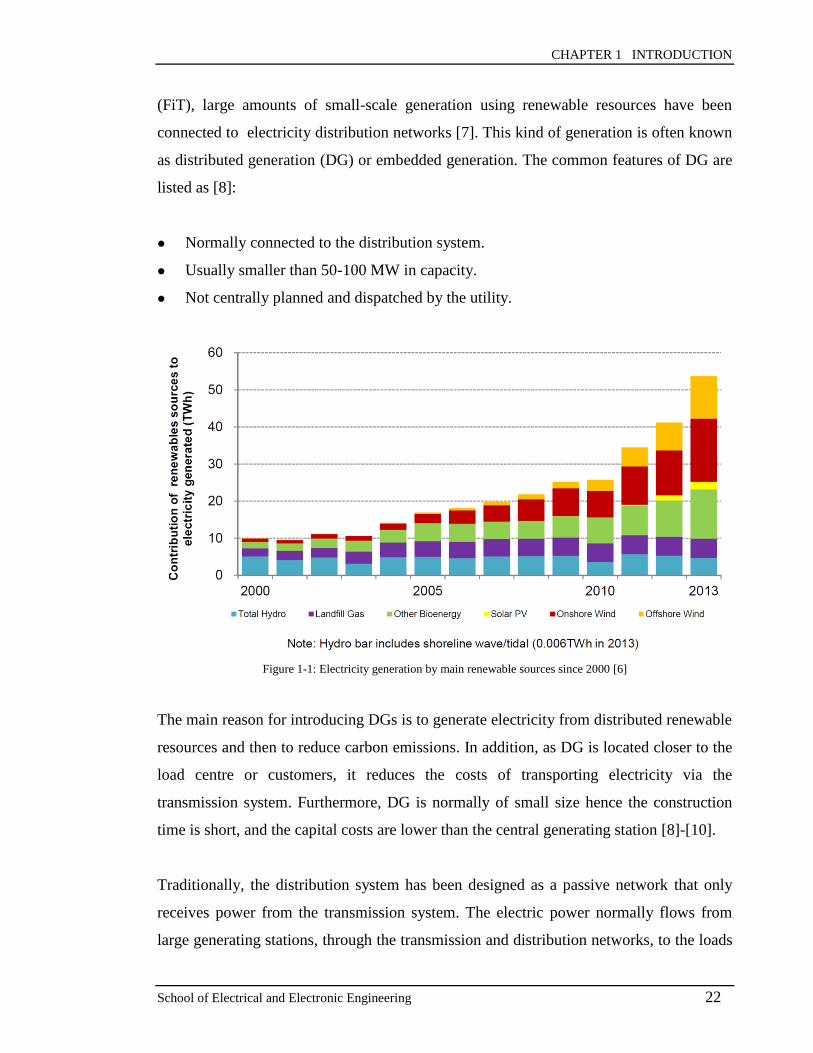
53.7 terawatt hours (TWh), taking a 14.9% share of the total electricity generation [6].
The overall wind generation in 2013 was around 28.4 TWh, which was 206% higher than
2009 (as shown in Figure 1-1). For the solar photovoltaic (PV) schemes, the installed
capacity increased from 0.027 gigawatt (GW) in 2009 to 2.78 GW in 2013.
Due to the low-carbon incentives offered by the UK government, e.g. Feed-in Tariff
CHAPTER 1 INTRODUCTION
School of Electrical and Electronic Engineering 22
(FiT), large amounts of small-scale generation using renewable resources have been
connected to electricity distribution networks [7]. This kind of generation is often known
as distributed generation (DG) or embedded generation. The common features of DG are
listed as [8]:
Normally connected to the distribution system.
Usually smaller than 50-100 MW in capacity.
Not centrally planned and dispatched by the utility.
Figure 1-1: Electricity generation by main renewable sources since 2000 [6]
The main reason for introducing DGs is to generate electricity from distributed renewable
resources and then to reduce carbon emissions. In addition, as DG is located closer to the
load centre or customers, it reduces the costs of transporting electricity via the
transmission system. Furthermore, DG is normally of small size hence the construction
time is short, and the capital costs are lower than the central generating station [8]-[10].
Traditionally, the distribution system has been designed as a passive network that only
receives power from the transmission system. The electric power normally flows from
large generating stations, through the transmission and distribution networks, to the loads
CHAPTER 1 INTRODUCTION
School of Electrical and Electronic Engineering 23
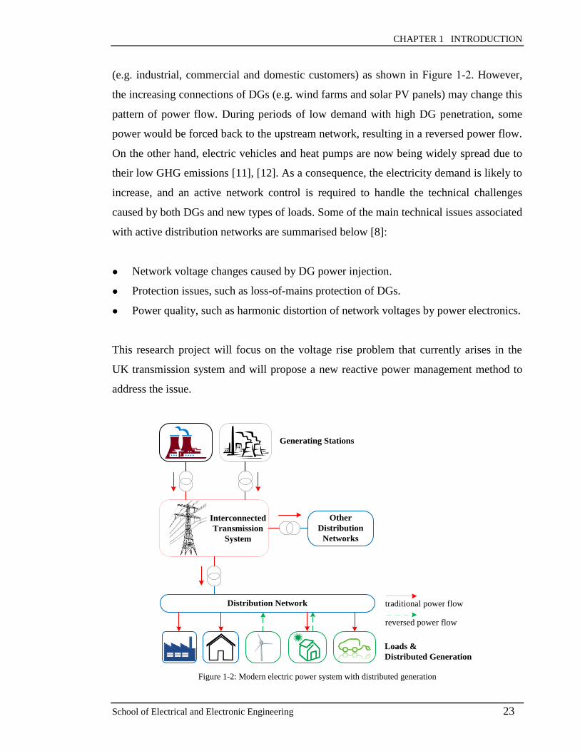
(e.g. industrial, commercial and domestic customers) as shown in Figure 1-2. However,
the increasing connections of DGs (e.g. wind farms and solar PV panels) may change this
pattern of power flow. During periods of low demand with high DG penetration, some
power would be forced back to the upstream network, resulting in a reversed power flow.
On the other hand, electric vehicles and heat pumps are now being widely spread due to
their low GHG emissions [11], [12]. As a consequence, the electricity demand is likely to
increase, and an active network control is required to handle the technical challenges
caused by both DGs and new types of loads. Some of the main technical issues associated
with active distribution networks are summarised below [8]:
Network voltage changes caused by DG power injection.
Protection issues, such as loss-of-mains protection of DGs.
Power quality, such as harmonic distortion of network voltages by power electronics.
This research project will focus on the voltage rise problem that currently arises in the
UK transmission system and will propose a new reactive power management method to
address the issue.
traditional power flow
reversed power flow
Distribution Network
Other
Distribution
Networks
Interconnected
Transmission
System
Generating Stations
Loads &
Distributed Generation
Figure 1-2: Modern electric power system with distributed generation

CHAPTER 1 INTRODUCTION
School of Electrical and Electronic Engineering 24
1.2 Voltage and Reactive Power Control
The electric power system is commonly a three-phase alternating-current (AC) system
comprising different voltage levels. To reduce transmission losses, the transmission
system is composed of lines with very high voltages. For the UK power system, the
typical transmission voltage levels are 400 kilovolts (kV), 275kV and 132kV (in Scotland)
[13], [14]. The distribution network voltages are normally 132kV, 33kV, 11kV, 6.6kV
and 400 volts (V). The line voltages change continuously with the varying electricity
demands. Network operators are responsible for maintaining the voltages high enough to
drive the loads while constraining the voltages to prevent equipment breakdown [15]. In
general, since the impedances of the network components are predominantly reactive,
voltage control is accomplished by managing the production, absorption and flow of
reactive power at all levels in the system [16]. The electrical load, e.g. motor, consumes
reactive power as well as active power. Network elements both consume and produce
reactive power. For instance, power transformers and overhead lines consume reactive
power. Lines and underground cables can also generate reactive power due to their shunt
capacitance [17]. However, the reactive power produced is only significant at high
system voltages or on light loads. During the steady-state operation of a power system,
the reactive power generation should match the load plus loss. An excess of reactive
power in an area may result in high voltages, or a deficit may lead to low voltages. The
relationship between reactive power and voltage is similar to the one between active
power and frequency.
Figure 1-3 illustrates a system with various components and devices combined to provide
voltage and reactive power (Volt/VAr) control. The network components or devices used
for Volt/VAr control may be summarised as follows [18]:
Generating units, such as synchronous generators.
Sources or sinks of reactive power, such as passive compensators including shunt
reactors and shunt capacitors, and active compensators including synchronous
condensers, static VAr compensators (SVCs) and static synchronous compensators

CHAPTER 1 INTRODUCTION
School of Electrical and Electronic Engineering 25
(STATCOMs).
Line reactance compensators, such as series capacitors.
Regulating transformers, such as on-load tap changer transformers.
Generating units
The generating units provide the primary voltage control in the system. Synchronous
generators are usually equipped with automatic voltage regulators (AVRs), which adjust
the field excitation to maintain the scheduled voltages at the terminals of the generators.
The control of excitation also determines whether the generators would produce or absorb
reactive power.
S
Generator
Series capacitor
Shunt reactor
Tap changing
transformer
Synchronous
condenser Shunt capacitor
Static VAr
compensator
Figure 1-3: Voltage and reactive power control with different components and devices in power system
Reactive power compensation devices
Due to the high reactance of network elements, reactive power cannot be transmitted
easily in the system. Voltage control has to be effected by distributing additional reactive
power compensation devices throughout the system [19], [20]. Shunt reactors and
capacitors provide passive compensation, which improves voltage profiles and reduces
system losses. They are either permanently connected to the transmission and distribution

CHAPTER 1 INTRODUCTION
School of Electrical and Electronic Engineering 26
systems, or switched. Series capacitors are installed to reduce the inductance of
transmission lines and to increase the power transfer capability. Synchronous condensers,
SVCs and STATCOMs provide active compensation. The produced or absorbed reactive
power is automatically adjusted to maintain constant voltages at the connecting buses.
The active compensating devices and generating units together establish voltages at
specific points in the system. Voltages at other locations are determined by the active and
reactive power flows in the circuit.
Regulating transformers
Transformers with tap-changing facilities are also widely used to regulate voltages in the
system at various voltage levels. The changes of tap position will affect the terminal
voltages and also the reactive power flow through the transformer. There are two types of
tap changer: off-load and on-load. The transformers with on-load tap changers (OLTCs)
can regulate voltages under varying load conditions without interruption. For the UK
transmission system, autotransformers connecting a 400kV or 275kV network to a 132kV
or 66kV network are usually equipped with OLTCs [18]. In distribution networks,
primary substation transformers (33/11 kV or 33/6.6 kV) are usually fitted with OLTCs
[21].
1.3 Motivation
One of the important problems concerning the integration of DGs into power systems is
the voltage rise issue. At the connection point (or Point of Common Coupling), DG starts
to boost the local voltage by injecting real power. However, the current distribution
network operator (DNO) policy is based on the “fit and forget” approach, which requires
DG to operate at a fixed power factor (e.g. unity power factor) without regulating reactive
power to control the voltage [22], [23]. This practice certainly limits the capacity of DG
connected and worsens the voltage rise effect. The voltage may sometimes rise over the
maximum statutory limit and damage devices at customer sides. In [24], some case
studies have demonstrated the voltage rise issue encountered at distribution networks.

CHAPTER 1 INTRODUCTION
School of Electrical and Electronic Engineering 27
The voltage rise problem can also occur in the transmission system. According to
National Grid Electricity Ten Year Statements [25] and [26], high voltage situations
under low demand conditions are currently increasing in the UK transmission grid. The
main reasons include:
Development of underground cables in transmission and distribution networks.
Decommissioning of coal generators in specific areas, resulting in a lack of generator
voltage control.
Reduction in reactive power demand during periods of minimum load.
Underground cables commonly have large capacitance, which produces excess reactive
power when the system is lightly loaded. The growing connection of large offshore wind
farms to the grid would require more submarine cables to be installed, which may also
cause voltages to rise if without proper VAr compensation [27]-[29].
In addition, National Grid, the Great Britain (GB) transmission system operator, has
reported the gradual decline in reactive power demand during minimum load periods (e.g.
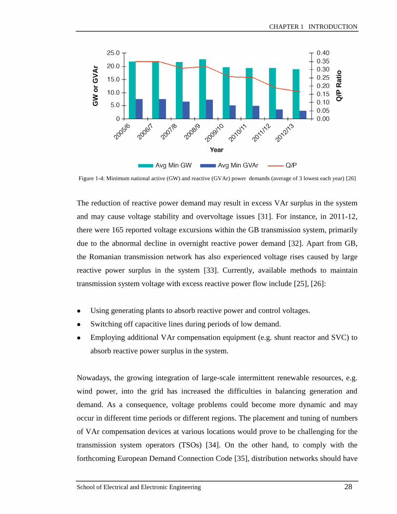
summer nights). Figure 1-4 demonstrates the historical trend of minimum active and
reactive power demands for the GB transmission system since 2005 [26]. The figure also
shows that the ratio between minimum reactive power and active power demands (Q/P
ratio) decreased by almost half from 2005 to 2012. During periods of low demand,
National Grid has observed low reactive power demand or even reactive power injection
at several Grid Supply Points (GSPs), where distribution networks are connected to the
GB transmission system. In some cases, reactive power has been exported from
distribution networks back to the transmission grid. The reasons behind this declining
trend of reactive power demand during minimum load periods are still uncertain. The
development of underground cables in distribution networks, the use of more energy-
efficient household appliances and the impact of DGs are some of the possible factors
affecting the system VAr demand. National Grid has carried out further investigations to
understand the exact cause of the reduction in reactive power demand [30].
CHAPTER 1 INTRODUCTION
School of Electrical and Electronic Engineering 28
GW
or
GV
Ar
Q/P
Ra
tio
Figure 1-4: Minimum national active (GW) and reactive (GVAr) power demands (average of 3 lowest each year) [26]
The reduction of reactive power demand may result in excess VAr surplus in the system
and may cause voltage stability and overvoltage issues [31]. For instance, in 2011-12,
there were 165 reported voltage excursions within the GB transmission system, primarily
due to the abnormal decline in overnight reactive power demand [32]. Apart from GB,
the Romanian transmission network has also experienced voltage rises caused by large
reactive power surplus in the system [33]. Currently, available methods to maintain
transmission system voltage with excess reactive power flow include [25], [26]:
Using generating plants to absorb reactive power and control voltages.
Switching off capacitive lines during periods of low demand.
Employing additional VAr compensation equipment (e.g. shunt reactor and SVC) to
absorb reactive power surplus in the system.
Nowadays, the growing integration of large-scale intermittent renewable resources, e.g.
wind power, into the grid has increased the difficulties in balancing generation and
demand. As a consequence, voltage problems could become more dynamic and may
occur in different time periods or different regions. The placement and tuning of numbers
of VAr compensation devices at various locations would prove to be challenging for the
transmission system operators (TSOs) [34]. On the other hand, to comply with the
forthcoming European Demand Connection Code [35], distribution networks should have
CHAPTER 1 INTRODUCTION
School of Electrical and Electronic Engineering 29
the capability to maintain a limited range of reactive power consumption at interfaces
with transmission systems. The rapid development of smart grid technologies would
facilitate the demand side response control in distribution networks. Therefore,
considering the VAr management challenges from both the transmission and distribution
sides, this study will concentrate on developing a cost-effective means of utilising
distribution networks to provide reactive power support for transmission systems.
1.4 Research Objectives
To mitigate the aforementioned reactive power surplus in transmission systems during
periods of low demand, traditional solutions often involve installing shunt reactors or
VAr compensators. The associated costs will be high if numbers of devices need to be
placed at various locations in the system. One alternative method is to increase the
reactive power consumption of the downstream connected distribution networks. The
operation of parallel transformers in different tap positions, i.e. with staggered taps, will
introduce a circulating current around the pair. Due to the transformer inductance, the
circulating current will draw more reactive power from the upstream network. For each
pair, the difference in tap positions should be set within a small range to avoid the
transformer overheating. However, the aggregated reactive power absorption from many
pairs of parallel transformers within the distribution networks may be sufficient to
provide VAr support to the upstream transmission system.
Therefore, the research objective is to develop a reactive power control method that
utilises the existing parallel transformers in distribution networks to provide VAr
supports for transmission systems. The outcomes may contribute to creating a new
business opportunity for distribution networks to participate in the reactive power
balancing services in the future. The smart management of distribution networks may
also enhance the reliability and stability of the transmission grid. Based on this concept,
the main research tasks are listed as follows:
Literature survey on recent Volt/VAr control development in transmission and
CHAPTER 1 INTRODUCTION
School of Electrical and Electronic Engineering 30
distribution systems, especially on the technologies to reduce reactive power surplus.
Modelling of typical UK High Voltage (HV) distribution networks, from 132kV
GSPs down to 33kV primary substations with parallel transformers.
Investigation of the reactive power absorption capability of the modelled distribution
networks with the tap staggering technique.
Development of a control algorithm to minimise the network loss and the number of
tap switching operations introduced when applying the tap staggering technique.
Test and comparison of the tap stagger control with other alternative algorithms and
distribution network models.
Modelling of a transmission system to analyse the consequential impacts of applying
the tap staggering method.
Assessment of both economic and dynamic effects of the tap staggering technique on
the transmission system.
Comparison with other VAr compensation methods used to reduce transmission
system VAr surplus.
1.5 List of Main Contributions to Work
The main contributions of this thesis are given below:
Propose a new reactive power control method, which utilises the existing parallel
transformers in distribution networks, to mitigate high voltages in transmission
systems during periods of low demand.
Assessment of the VAr absorption capability of a real UK HV distribution network
with the tap staggering technique.
Design of an optimal control approach based on genetic algorithm (GA) to
coordinate the tap staggering operation of multiple pairs of parallel transformers. An
objective function is proposed to minimise the introduced network loss as well as the
number of tap switching operations.
Comparison of the GA-based tap stagger control approach with two alternative
methods, i.e. the rule-based control scheme and the branch-and-bound method, using

CHAPTER 1 INTRODUCTION
School of Electrical and Electronic Engineering 31
two UK HV distribution network models.
Comparison of the impacts of the tap staggering technique and the use of shunt
reactors on transmission systems, in terms of economic costs and dynamic
performance.
1.6 Thesis Outline
The present Chapter 1 briefly introduces the background of power system voltage and
reactive power control, describes the research subject and motivation. Detailed research
objectives are listed along with the main contributions to the work. The remainder of this
thesis is organized as follows:
Chapter 2 presents a critical literature review of existing voltage and reactive power
control techniques in transmission and distribution systems, focusing on the steady-state
power flow control. Voltage regulation schemes with the presence of renewable energy
generation or DG are described. Different methods for reactive power management in
transmission systems are discussed. The optimisation algorithms for voltage and reactive
power control are also investigated to understand their working principles, advantages
and limitations. From the literature, an alternative reactive power management method to
mitigate reactive power surplus in the transmission system is proposed in Chapter 4.
Chapter 3 describes the fundamental theories related to the proposed reactive power
management method, for the purpose of a better understanding of the subsequent chapters.
It first presents the basic structure of distribution networks and the relationship between
voltage and reactive power control. Tap changer mechanisms and the load flow
modelling of the transformer with tap changer are given.
Chapter 4 proposes a reactive power control method, which utilises the existing parallel
transformers in distribution networks, to mitigate high voltages for transmission systems
during periods of low demand. The proposed ‘tap staggering’ method aims to use the tap
position differences of parallel transformers to introduce virtual inductive loading onto

CHAPTER 1 INTRODUCTION
School of Electrical and Electronic Engineering 32
the upstream system. The mathematical principles of the tap staggering operation are
discussed. An optimal control approach for the tap stagger is also proposed, which aims
to minimise the active network loss as well as the number of tap switching operations
introduced. The following Chapter 5 first presents the feasibility studies of assessing
distribution network reactive power absorption capabilities using the tap staggering
technique. Chapters 6 and 7 then describe the optimisation studies for the tap stagger with
different solution algorithms. Chapter 8 investigates the impacts of tap stagger on the
transmission system.
Chapter 5 presents the feasibility studies to investigate the VAr absorption capability of
distribution networks through the use of tap stagger. The modelled distribution system is
based on a real UK distribution network from the 132kV GSPs down to 33kV primary
substations with parallel transformers. Off-line load flow studies are carried out to
analyse the overall network VAr consumption as well as the power loss with tap stagger.
Chapter 6 describes the implementation of the tap stagger optimal control. As the
optimisation is an integer nonlinear problem, a genetic algorithm (GA) based procedure is
developed to find an optimal dispatch for the tap positions of the parallel transformers.
Studies are carried out to test the impacts of reactive power requirements, load models
and demand levels on the optimisation results. The comparisons with other solution
algorithms are given in Chapter 7.
Chapter 7 focuses on the comparisons of the tap stagger control with two other
alternative methods, i.e. the rule-based approach and the branch-and-bound algorithm.
Two practical UK distribution networks are modelled from real data and used to
demonstrate the effectiveness of the three control approaches with different input settings.
Chapter 8 presents both the economic and technical analyses of using the tap staggering
method. In the economic analysis, the associated costs of applying the tap staggering
technique are investigated through static load flow studies. The IEEE Reliability Test
System is used to carry out the studies, and the results are compared with the installation

CHAPTER 1 INTRODUCTION
School of Electrical and Electronic Engineering 33
of shunt reactors. In the technical studies, the dynamic impacts of tap staggering or
reactor switching on transmission voltages are analysed.
Chapter 9 draws conclusions from the work described in this thesis. The main findings
of the research are discussed, and possible directions for future work are suggested.

CHAPTER 2 LITERATURE REVIEW
School of Electrical and Electronic Engineering 34
CHAPTER 2
2 LITERATURE REVIEW
2.1 Introduction
This chapter presents different voltage and reactive power control methods that have been
currently applied to or proposed for power systems over the years. The review starts with
a discussion of traditional voltage regulation methods used in transmission or distribution
networks. This is followed by an overview of recent voltage control approaches
developed considering the integration of DG or renewable energy generation into the grid.
As this research project is concerned with the voltage problems due to reactive power
surplus in transmission systems, the existing reactive power compensation techniques for
transmission systems are presented and discussed. The related Volt/VAr optimisation
control schemes, which coordinate multiple VAr compensators to optimise network
performance, are also described. Finally, a summary is provided to comment on the
Volt/VAr control and the associated optimisation algorithms.
2.2 Traditional Voltage Regulation Methods
Both utility equipment and customer equipment that are connected to a power system are
designed to operate within a certain voltage range. To avoid any adverse effects on the
equipment caused by voltage violations, network operators are responsible for
maintaining the system voltages within statutory limits [36].
Since electricity loads continuously change, there must be some means of regulating
network voltages to satisfy the requirements. As described in Chapter 1, most voltage
control methods are based on the principle of managing reactive power flow in the
system. The details are given in the following text.

CHAPTER 2 LITERATURE REVIEW
School of Electrical and Electronic Engineering 35
2.2.1 Transmission system voltage control
2.2.1.1 Automatic voltage regulators
Generating units connected to the transmission grid provide the most elementary voltage
control for the system. The AVRs equipped on synchronous generators adjust the field
excitation to regulate the voltages at connected buses. Figure 2-1 illustrates the block
diagram of a typical AVR closed-loop control [37]. The AVR monitors the generator
terminal voltage V and compares it with a desired reference voltage Vr. The resulting
voltage error is then amplified and used to alter the exciter output, i.e. the generator field
current. To stabilise the excitation control system and improve its dynamic performance,
a derivative feedback is usually adopted as shown in Figure 2-1. The response time of the
AVR control is extremely rapid, within a time frame of a few seconds [38], [39].
Figure 2-1: Block diagram of a closed-loop automatic voltage regulator [37]
The control of excitation also affects the reactive power production of generators. When
underexcited, generators absorb reactive power, and they supply reactive power when
overexcited. The excitation system can be controlled to maintain constant reactive power
or power factor (PF) instead of constant terminal voltage. However, compared with the
AVR controllers, the VAr/PF controllers should generally not be installed on generators
that intend to provide voltage support for transmission systems. The VAr/PF controllers
will prevent necessary reactive power changes during long periods of system voltage
excursions [40].
CHAPTER 2 LITERATURE REVIEW
School of Electrical and Electronic Engineering 36
2.2.1.2 Secondary voltage control
The generators with AVRs provide the primary voltage control, which aims to
compensate the rapid and random voltage variations at the locally connected buses. To
handle slow and large voltage variations (e.g. caused by demand changes), secondary
voltage control has been implemented in some European countries, such as France [41],
[42] and Italy [43], [44]. The principle of secondary voltage control is to divide a
transmission network into several uncoupled zones and to control the voltage profile
separately in each zone. A pilot bus is selected as a representative bus for each zone and
the bus voltage is controlled via automatic adjustments of the AVRs of several generators
located in the zone.
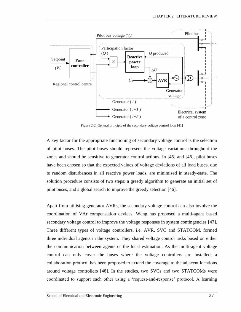
The main objectives of secondary voltage control are to maintain the pilot bus voltage at
a specified value and to coordinate reactive power sources within a control zone. Figure
2-2 shows how to perform the control [41]. The zone controller located in the regional
control centre acquires the pilot bus measured voltage Vp and compares it with a
predefined reference Vc. According to the voltage error, a control signal is generated and
transmitted to each controlling generator inside the zone. For each generator, the control
signal is multiplied by a corresponding participation factor Qr and the result is used as the
input to a reactive power control loop. The loop is designed to regulate the generator VAr
production by adjusting the AVR voltage reference. The secondary voltage control closes
the control loop of the reference settings of AVRs at the primary level. It also provides an
essential coordination of the reactive power of different controlling generators. The
response time is typically in the range of 3 minutes [39].
CHAPTER 2 LITERATURE REVIEW
School of Electrical and Electronic Engineering 37
Zone
controller
Setpoint
(Vc)
×
Reactive
power
loop
AVR×
Pilot bus voltage (Vp)
Generator ( i )
Participation factor
(Qr) Q produced
∆U
U0
Generator
voltage
Pilot bus
×
×
×
×
×
×
Generator ( i+1 )
Generator ( i+2 )Electrical system
of a control zone
Regional control centre
Figure 2-2: General principle of the secondary voltage control loop [41]
A key factor for the appropriate functioning of secondary voltage control is the selection
of pilot buses. The pilot buses should represent the voltage variations throughout the
zones and should be sensitive to generator control actions. In [45] and [46], pilot buses
have been chosen so that the expected values of voltage deviations of all load buses, due
to random disturbances in all reactive power loads, are minimised in steady-state. The
solution procedure consists of two steps: a greedy algorithm to generate an initial set of
pilot buses, and a global search to improve the greedy selection [46].
Apart from utilising generator AVRs, the secondary voltage control can also involve the
coordination of VAr compensation devices. Wang has proposed a multi-agent based
secondary voltage control to improve the voltage responses in system contingencies [47].
Three different types of voltage controllers, i.e. AVR, SVC and STATCOM, formed
three individual agents in the system. They shared voltage control tasks based on either
the communication between agents or the local estimation. As the multi-agent voltage
control can only cover the buses where the voltage controllers are installed, a
collaboration protocol has been proposed to extend the coverage to the adjacent locations
around voltage controllers [48]. In the studies, two SVCs and two STATCOMs were
coordinated to support each other using a ‘request-and-response’ protocol. A learning

CHAPTER 2 LITERATURE REVIEW
School of Electrical and Electronic Engineering 38
fuzzy logic controller was designed to implement the control algorithm for each voltage
controller.
2.2.1.3 Coordinated secondary voltage control & tertiary voltage control
The secondary voltage control only maintains the voltage profile inside a control zone.
Considering the interaction between zones, the concept of coordinated secondary voltage
control (CSVC) has been introduced [38]. The control strategy relies on the partition of a
network into regions, which are much larger than zones and include more than one pilot
bus. In each control region, the CSVC aims to control the voltages of pilot buses and to
maintain the reactive power generation of each controlling generator at a reference value.
The control variables are the AVR voltage setpoints and are obtained as the solutions of
an optimisation problem, which minimises the sum of pilot bus voltage deviations and
generator VAr productions, subject to various network constraints. In [49], a
decentralised control approach for CSVC has been presented concerning the VAr
compensation from neighbourhood regions. If a control region has voltage violations due
to load disturbances, the CSVC controllers located at pilot buses will first employ
generators or VAr compensators to regulate the voltages. In a severe contingency when
the disturbed region requires more reactive power, the CSVC controllers in
neighbourhood regions can transfer their extra reactive power to the affected region. To
achieve this control strategy, connection matrices were used to represent the possible
coordination between controllers in a region or different regions.
Voltage setpoints of pilot buses can be determined by the tertiary voltage control (TVC).
At the national level, the TVC utilises the global information of the transmission grid,
and it updates the reference values for the secondary voltage control by solving
optimisation problems [43], [50] and [51]. The optimal voltage setpoints for pilot buses
are determined to minimise the grid losses while still preserving a sufficiently reactive
power margin. In the short term, the optimisation program can be carried out one day in
advance based on load forecasting. Alternatively, in the very short term, the program can
run every 15-30 minutes using the online state estimation [43], [44].
CHAPTER 2 LITERATURE REVIEW
School of Electrical and Electronic Engineering 39
2.2.2 Distribution system voltage control
As distribution systems have traditionally been designed as passive networks without
connections to large generating plants, the voltage regulation often considers the use of
reactive power compensation devices or tap changing transformers. The details are given
in the following text.
2.2.2.1 Common voltage control techniques for distribution networks
A number of techniques is available for the voltage regulation in distribution networks.
Some common methods are listed as [52], [53]:
Installing reactive power compensation devices (e.g. shunt capacitors).
Building new substations and primary feeders.
Increasing the conductor size of existing feeders.
Rearranging the system, transferring loads.
Adding series capacitors to the primary feeders.
Utilising substation transformers with on-load/off-load tap changers.
Applying voltage regulators on the primary feeders.
The application of reactive power compensation equipment, e.g. shunt capacitor and
reactor, synchronous condenser and static var compensator (SVC), is able to provide the
reactive power locally when demand is high or to absorb the reactive power when
demand is low. They can be installed at different locations in distribution systems to
ensure the voltages remain within the permitted range as the loads vary. In addition, the
locations and VAr outputs of compensators can be optimised to minimise the network
losses and improve the efficiency.
The building of new substations and primary feeders intends to reduce the power flow on
each line so that less voltage drop (or rise) is introduced. Similarly, the voltage drop can
also be reduced by decreasing the line impedance (e.g. increasing the conductor size or
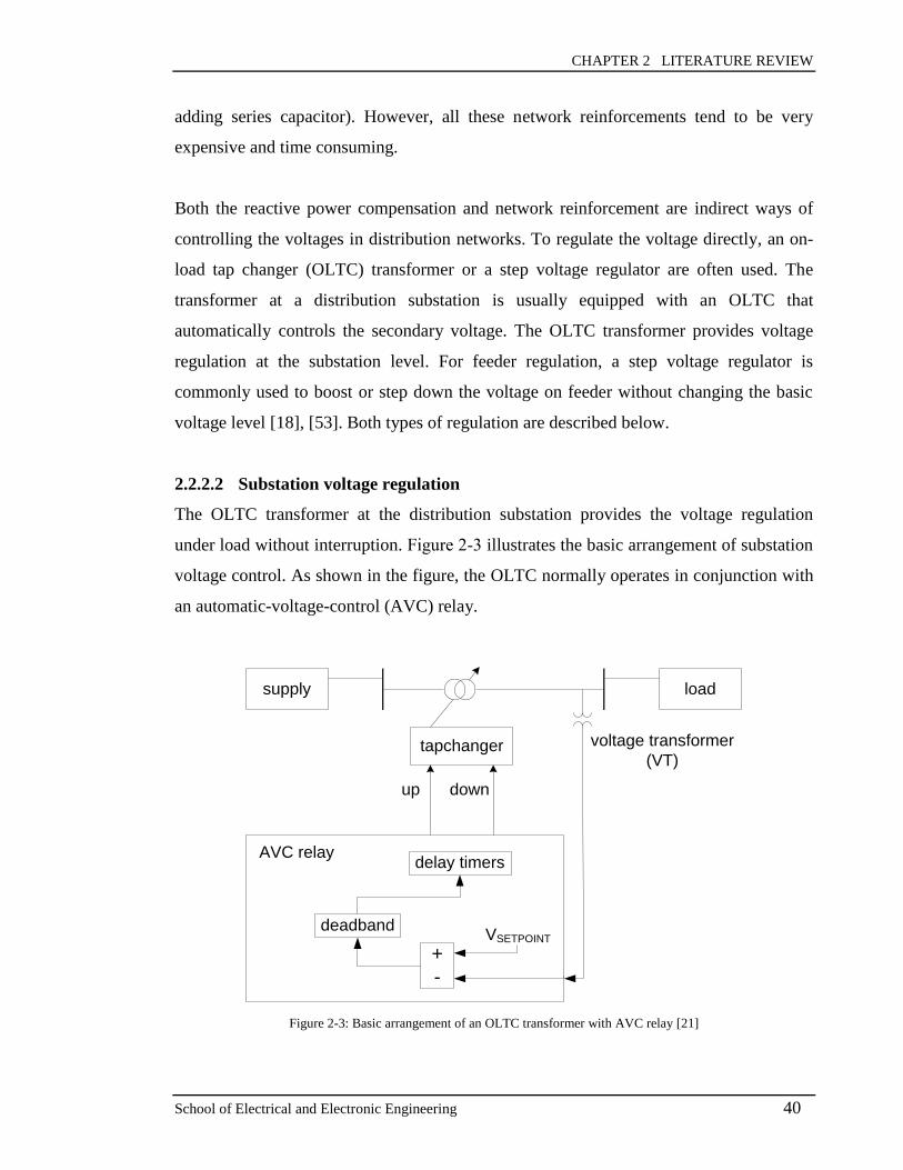
CHAPTER 2 LITERATURE REVIEW
School of Electrical and Electronic Engineering 40
adding series capacitor). However, all these network reinforcements tend to be very
expensive and time consuming.
Both the reactive power compensation and network reinforcement are indirect ways of
controlling the voltages in distribution networks. To regulate the voltage directly, an on-
load tap changer (OLTC) transformer or a step voltage regulator are often used. The
transformer at a distribution substation is usually equipped with an OLTC that
automatically controls the secondary voltage. The OLTC transformer provides voltage
regulation at the substation level. For feeder regulation, a step voltage regulator is
commonly used to boost or step down the voltage on feeder without changing the basic
voltage level [18], [53]. Both types of regulation are described below.
2.2.2.2 Substation voltage regulation
The OLTC transformer at the distribution substation provides the voltage regulation
under load without interruption. Figure 2-3 illustrates the basic arrangement of substation
voltage control. As shown in the figure, the OLTC normally operates in conjunction with
an automatic-voltage-control (AVC) relay.
supply load
tapchanger
up down
AVC relay
+
-
VSETPOINTdeadband
delay timers
voltage transformer
(VT)
Figure 2-3: Basic arrangement of an OLTC transformer with AVC relay [21]
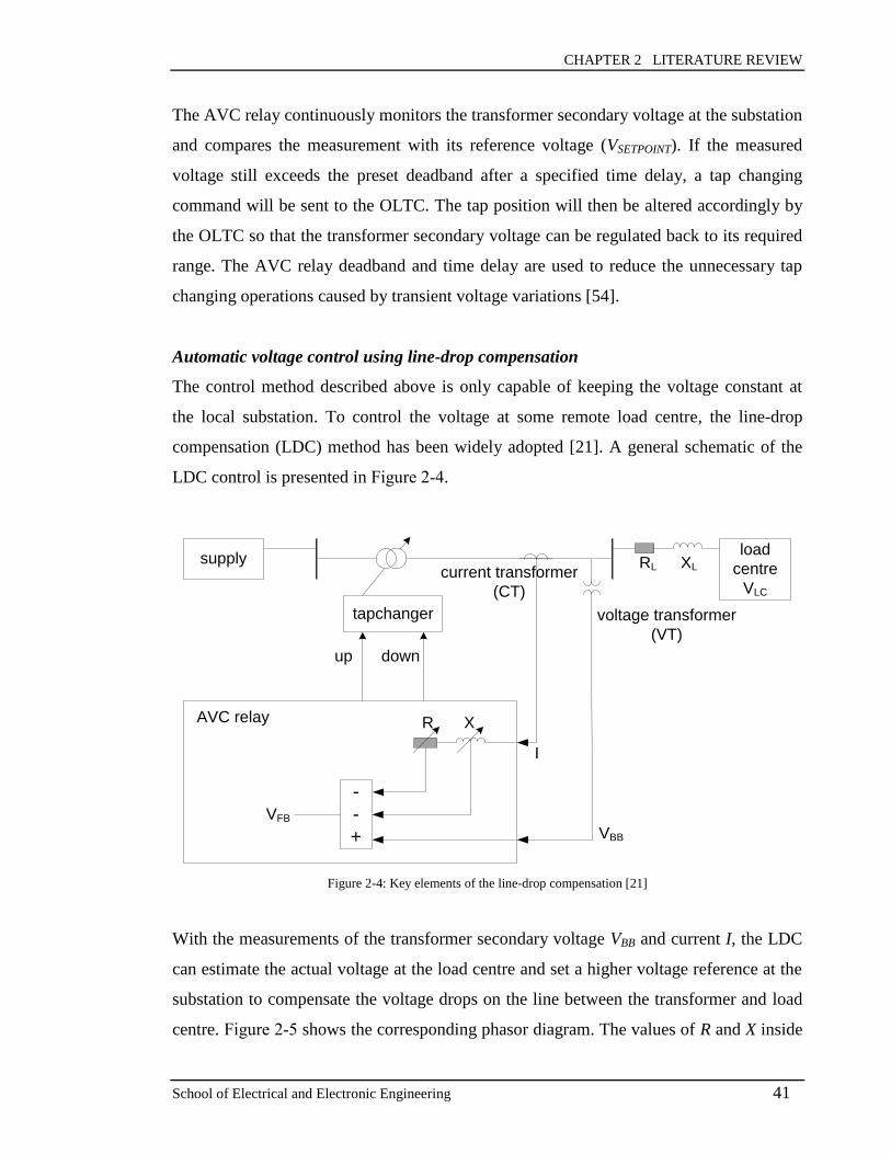
CHAPTER 2 LITERATURE REVIEW
School of Electrical and Electronic Engineering 41
The AVC relay continuously monitors the transformer secondary voltage at the substation
and compares the measurement with its reference voltage (VSETPOINT). If the measured
voltage still exceeds the preset deadband after a specified time delay, a tap changing
command will be sent to the OLTC. The tap position will then be altered accordingly by
the OLTC so that the transformer secondary voltage can be regulated back to its required
range. The AVC relay deadband and time delay are used to reduce the unnecessary tap
changing operations caused by transient voltage variations [54].
Automatic voltage control using line-drop compensation
The control method described above is only capable of keeping the voltage constant at
the local substation. To control the voltage at some remote load centre, the line-drop
compensation (LDC) method has been widely adopted [21]. A general schematic of the
LDC control is presented in Figure 2-4.
supplyload
centre
VLC
tapchanger
up down
AVC relay
-
-
+
VFB
voltage transformer
(VT)
RL XL
I
VBB
R X
current transformer
(CT)
Figure 2-4: Key elements of the line-drop compensation [21]
With the measurements of the transformer secondary voltage VBB and current I, the LDC
can estimate the actual voltage at the load centre and set a higher voltage reference at the
substation to compensate the voltage drops on the line between the transformer and load
centre. Figure 2-5 shows the corresponding phasor diagram. The values of R and X inside
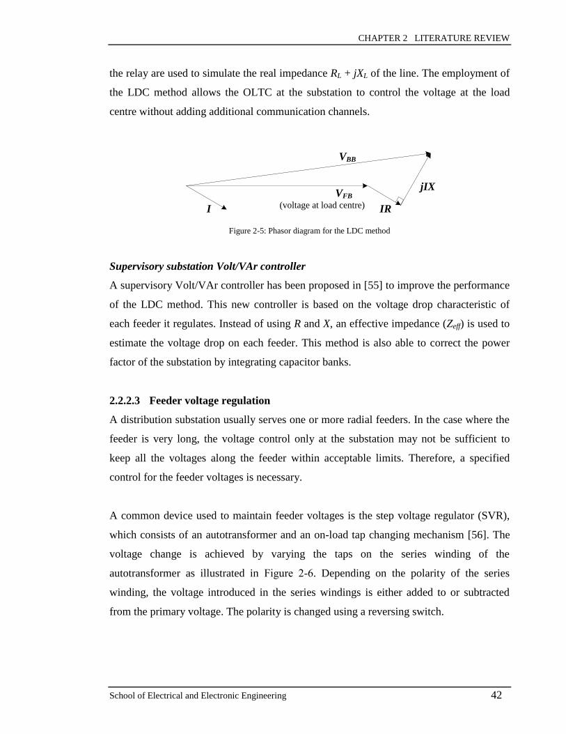
CHAPTER 2 LITERATURE REVIEW
School of Electrical and Electronic Engineering 42
the relay are used to simulate the real impedance RL + jXL of the line. The employment of
the LDC method allows the OLTC at the substation to control the voltage at the load
centre without adding additional communication channels.
VBB
I
VFB
IR
jIX
(voltage at load centre)
Figure 2-5: Phasor diagram for the LDC method
Supervisory substation Volt/VAr controller
A supervisory Volt/VAr controller has been proposed in [55] to improve the performance
of the LDC method. This new controller is based on the voltage drop characteristic of
each feeder it regulates. Instead of using R and X, an effective impedance (Zeff) is used to
estimate the voltage drop on each feeder. This method is also able to correct the power
factor of the substation by integrating capacitor banks.
2.2.2.3 Feeder voltage regulation
A distribution substation usually serves one or more radial feeders. In the case where the
feeder is very long, the voltage control only at the substation may not be sufficient to
keep all the voltages along the feeder within acceptable limits. Therefore, a specified
control for the feeder voltages is necessary.
A common device used to maintain feeder voltages is the step voltage regulator (SVR),
which consists of an autotransformer and an on-load tap changing mechanism [56]. The
voltage change is achieved by varying the taps on the series winding of the
autotransformer as illustrated in Figure 2-6. Depending on the polarity of the series
winding, the voltage introduced in the series windings is either added to or subtracted
from the primary voltage. The polarity is changed using a reversing switch.
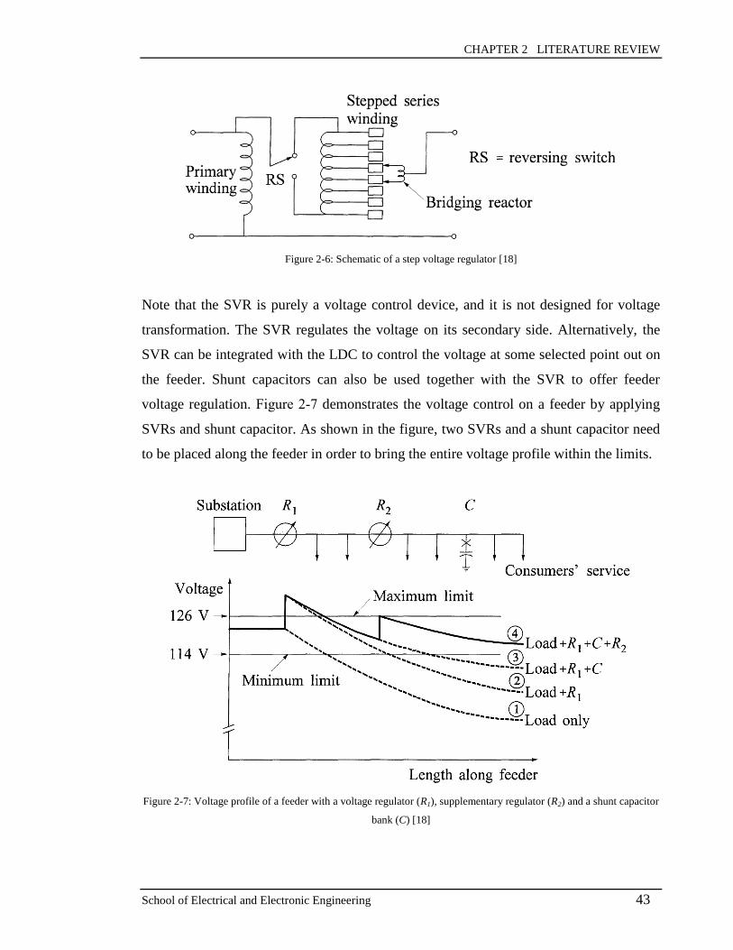
CHAPTER 2 LITERATURE REVIEW
School of Electrical and Electronic Engineering 43
Figure 2-6: Schematic of a step voltage regulator [18]
Note that the SVR is purely a voltage control device, and it is not designed for voltage
transformation. The SVR regulates the voltage on its secondary side. Alternatively, the
SVR can be integrated with the LDC to control the voltage at some selected point out on
the feeder. Shunt capacitors can also be used together with the SVR to offer feeder
voltage regulation. Figure 2-7 demonstrates the voltage control on a feeder by applying
SVRs and shunt capacitor. As shown in the figure, two SVRs and a shunt capacitor need
to be placed along the feeder in order to bring the entire voltage profile within the limits.
Figure 2-7: Voltage profile of a feeder with a voltage regulator (R1), supplementary regulator (R2) and a shunt capacitor
bank (C) [18]

CHAPTER 2 LITERATURE REVIEW
School of Electrical and Electronic Engineering 44
2.3 Voltage Control Methods with Distributed Generation
As mentioned in Chapter 1, the growing integration of renewable energy generation into
grids may cause voltage problems on the existing power systems. For transmission
networks, the connection of large-scale intermittent renewable resources, e.g. wind power,
increases the difficulties in balancing generation and demand. For distribution systems,
small variable DGs (e.g. solar PV panels) have been connected to the networks, which
may change or even reverse the power flows at the points of connection. The traditional
voltage control schemes designed for the passive system with unidirectional power flow
may become inadequate [57]. The electricity generation of DGs may also be limited due
to the voltage violations caused. Considering the voltage issues, the network management
system design will need to be transferred from the traditional ‘passive’ network control to
a fully ‘active’ network operation in the future. The following literature reviews present
several voltage regulation methods associated with renewable energy generation,
concentrating mostly on distribution systems. The control principles can be divided into
three main parts: on-load tap changer control, reactive power control and power
curtailment. The details are given below.
2.3.1 On-load tap changer control
The traditional substation voltage control with the LDC algorithm is designed for the
passive network with the unidirectional power flow. In the active distribution network
with DGs injecting current to the feeder, the current measured at the substation is no
longer proportional to the load current. As a consequence, the LDC method using current
measurements becomes less effective at regulating the voltage at the load centre [21].
Alternative control techniques utilising OLTC transformers have been proposed for the
active network.
2.3.1.1 SuperTAPP n+ relay scheme
In [58] and [59], SuperTAPP n+ relay scheme has been introduced to control the voltage
in the network with DGs. This type of relay is capable of estimating the output current of
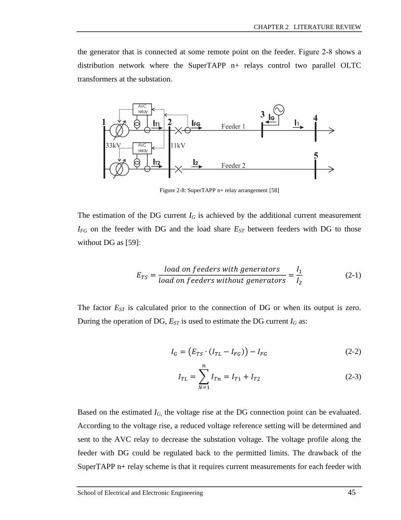
CHAPTER 2 LITERATURE REVIEW
School of Electrical and Electronic Engineering 45
the generator that is connected at some remote point on the feeder. Figure 2-8 shows a
distribution network where the SuperTAPP n+ relays control two parallel OLTC
transformers at the substation.
Figure 2-8: SuperTAPP n+ relay arrangement [58]
The estimation of the DG current IG is achieved by the additional current measurement
IFG on the feeder with DG and the load share EST between feeders with DG to those
without DG as [59]:
𝐸𝑇𝑆 =𝑙𝑜𝑎𝑑 𝑜𝑛 𝑓𝑒𝑒𝑑𝑒𝑟𝑠 𝑤𝑖𝑡ℎ 𝑔𝑒𝑛𝑒𝑟𝑎𝑡𝑜𝑟𝑠
𝑙𝑜𝑎𝑑 𝑜𝑛 𝑓𝑒𝑒𝑑𝑒𝑟𝑠 𝑤𝑖𝑡ℎ𝑜𝑢𝑡 𝑔𝑒𝑛𝑒𝑟𝑎𝑡𝑜𝑟𝑠=
𝐼1𝐼2
(2-1)
The factor EST is calculated prior to the connection of DG or when its output is zero.
During the operation of DG, EST is used to estimate the DG current IG as:
𝐼𝐺 = (𝐸𝑇𝑆 ∙ (𝐼𝑇𝐿 − 𝐼𝐹𝐺)) − 𝐼𝐹𝐺 (2-2)
𝐼𝑇𝐿 = ∑ 𝐼𝑇𝑛
𝑛
𝑁=1
= 𝐼𝑇1 + 𝐼𝑇2 (2-3)
Based on the estimated IG, the voltage rise at the DG connection point can be evaluated.
According to the voltage rise, a reduced voltage reference setting will be determined and
sent to the AVC relay to decrease the substation voltage. The voltage profile along the
feeder with DG could be regulated back to the permitted limits. The drawback of the
SuperTAPP n+ relay scheme is that it requires current measurements for each feeder with

CHAPTER 2 LITERATURE REVIEW
School of Electrical and Electronic Engineering 46
DG. This may increase the control costs and response time when there are multiple
feeders connected with DGs.
2.3.1.2 Automatic voltage reference setting using state estimation
For the OLTC control, the voltage reference setting of the AVC relay can be determined
using the LDC method or the aforementioned SuperTAPP n+ relay scheme. Alternatively,
El-Feres and Li have proposed an automatic voltage reference setting technique based on
distribution state estimation (DSE) [60]. The DSE is a mathematical minimisation
process used to estimate bus voltages in distribution networks. A weighted least square
function is commonly adopted to formulate the state estimation as [61], [62]:
min𝒙
𝐽(𝒙) = ∑[𝑧𝑖
𝑚𝑒𝑎𝑠 − 𝑓𝑖(𝒙)]2
𝜎𝑖2
𝑁𝑚
𝑖=1
(2-4)
where,
x State vector that consists of network bus voltages.
Nm Total number of measurements.
𝑧𝑖𝑚𝑒𝑎𝑠 The i
th measurement value.
𝑓𝑖(𝒙) A function of state variables and it is used to calculate the theoretical value of
the ith
measurement.
𝜎𝑖2 Variance of the i
th measurement.
The solution of Equation (2-4) is a set of state variables that minimises the squares of
errors between the measured values and the values calculated from state variables. In
other words, the DSE can generate a group of bus voltages that enables the power flow
calculated in theory to match the measurements. To reduce the needs of a large number of
measurements, the DSE only takes real-time measurements at critical points in the
network and combines them with pseudo measurements [63], [64]. The pseudo
measurements can be obtained from historical load flow data of substation transformers.
CHAPTER 2 LITERATURE REVIEW
School of Electrical and Electronic Engineering 47
With the DSE, the voltage controller at the substation can observe the voltage changes of
the downstream feeders due to DG penetration. The AVC target voltage can then be
updated to adjust the substation voltage accordingly. In [60], a real-time closed-loop
testing facility has also been developed to investigate the behaviours of the DSE based
voltage controller under different load and DG conditions.
2.3.1.3 Impact of wind power variability on transformer tap operations
Due to the fluctuating nature of wind power, the power output from wind turbines may
introduce high power flow fluctuations through the substation transformers. This may
ultimately lead to an increase in the frequency of tap changes and reduce the lifetime of
tap changers. In [65], the corresponding analysis has been carried out for the wind farms
connected to a meshed sub-transmission system. The result indicates that the wind power
injection has increased the number of tap changing operations. The increase is found to
be significant when the wind farm provides local voltage regulation. To reduce the
number of tap changes introduced at the substation transformer, a control algorithm
utilising the reactive power compensation from local wind turbines has been proposed in
[66].
2.3.2 Reactive power control
Reactive power management provides the other way to address the voltage issue due to
DG penetration. At the point of connection, voltage variations could be compensated by
controlling the reactive power of DG [57]. A range of methods based on reactive power
control has been proposed to raise the level of distributed generation that could be
connected to the network.
2.3.2.1 Generator reactive power control
In [67], a distributed reactive power generation control has been developed for the DG to
alleviate the voltage rise issue (see Figure 2-9). Instead of directly regulating the bus
voltage at the connection point, the proposed method aims to minimise the voltage rise by
controlling the reactive power absorption of DG. The reference setting of the DG reactive
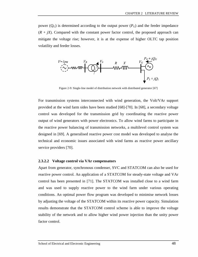
CHAPTER 2 LITERATURE REVIEW
School of Electrical and Electronic Engineering 48
power (QG) is determined according to the output power (PG) and the feeder impedance
(R + jX). Compared with the constant power factor control, the proposed approach can
mitigate the voltage rise; however, it is at the expense of higher OLTC tap position
volatility and feeder losses.
Figure 2-9: Single-line model of distribution network with distributed generator [67]
For transmission systems interconnected with wind generation, the Volt/VAr support
provided at the wind farm sides have been studied [68]-[70]. In [68], a secondary voltage
control was developed for the transmission grid by coordinating the reactive power
output of wind generators with power electronics. To allow wind farms to participate in
the reactive power balancing of transmission networks, a multilevel control system was
designed in [69]. A generalised reactive power cost model was developed to analyse the
technical and economic issues associated with wind farms as reactive power ancillary
service providers [70].
2.3.2.2 Voltage control via VAr compensators
Apart from generator, synchronous condenser, SVC and STATCOM can also be used for
reactive power control. An application of a STATCOM for steady-state voltage and VAr
control has been presented in [71]. The STATCOM was installed close to a wind farm
and was used to supply reactive power to the wind farm under various operating
conditions. An optimal power flow program was developed to minimise network losses
by adjusting the voltage of the STATCOM within its reactive power capacity. Simulation
results demonstrate that the STATCOM control scheme is able to improve the voltage
stability of the network and to allow higher wind power injection than the unity power
factor control.
CHAPTER 2 LITERATURE REVIEW
School of Electrical and Electronic Engineering 49
2.3.2.3 Network losses affected by reactive power control
The reactive power flow changes due to VAr compensation may have impacts on the
system losses. A significant amount of reactive power compensation may increase the
line current, resulting in higher transmission losses in the network. Considering the
presence of DGs, an optimisation algorithm has been developed to minimise the network
losses while keeping bus voltages within limits [72]. The control variables are the active
(PDG) and reactive power (QDG) output from each DG. More details about the Volt/VAr
optimisation control will be given in Section 2.5.
2.3.3 Power curtailment
Active power curtailment of DG has been proposed as another way to mitigate the
voltage rise issue. If the bus voltage at the connection point is approaching the upper limit
when demand is low, the generator can reduce its output by a certain amount so that the
voltage is still maintained below the limit. This will allow the generator to keep operating
rather than being tripped off from the network by the DNO. The generator can increase
its output again under normal or heavy load conditions. Therefore, it may be profitable
for the DG to curtail some of its output power for a limited period if that allows the DG to
connect larger capacity.
2.3.3.1 Power curtailment cost minimisation
Liew and Strbac have developed an optimal power flow (OPF) algorithm to minimise the
annual active power curtailment cost of embedded wind generation [57]. The reference
settings of the generation curtailment, the reactive power compensation and the OLTC
tap positions are combined as the control variables of the OPF algorithm. Case studies
show that the proposed control scheme can increase the installed capacity of wind
generation without violating voltage limits. The revenue lost due to the power curtailment
can be maintained within a reasonable range for low levels of wind penetration (e.g.
installed capacity less than 1 MW in the case studies). However, as the penetration level
increases, the revenue lost and the curtailed energy increase considerably and these may
no longer be acceptable.

CHAPTER 2 LITERATURE REVIEW
School of Electrical and Electronic Engineering 50
2.3.3.2 Active power control of DG
In [73], an active power control approach has been proposed for PVs to provide local
voltage regulation. This method is designed for the low voltage (LV) feeder with PV
integration as shown in Figure 2-10.
PVPVPV
Figure 2-10: Low voltage feeder with PVs [73]
The traditional control based on the maximum power point tracker allows the PV to inject
all the power made available by the photovoltaic array. However, the PV may be
switched off by the DNO if overvoltages occur at the point of connection. In the proposed
method, the traditional control has been integrated with an active power curtailment
control, which regulates the active power generation according to the local bus voltage.
The PV can be switched from the traditional control mode to the power curtailment
control mode, depending on the network operating conditions. Another generation control
of DG has been presented in [74]. For this design, the active power control of the
generator is used to provide supports for the voltage regulation only when the reactive
power control becomes insufficient to keep the voltage as the generator reaches its
reactive power limit.
2.4 Reactive Power Management in Transmission Systems
The aim of this project is to develop a reactive power control approach, which can help
maintain the voltages of transmission systems during periods of low demand. The
existing methods for reactive power management in transmission systems have therefore
been reviewed in terms of their methodologies, advantages and limitations. The
alternative reactive power control technique will be proposed based on the literature.

CHAPTER 2 LITERATURE REVIEW
School of Electrical and Electronic Engineering 51
2.4.1 Generation and absorption of reactive power
At present, transmission systems employ synchronous generators, capacitors, reactors,
synchronous condensers, SVCs and STATCOMs to control the reactive power flow.
Synchronous generators are frequently used to produce or absorb reactive power
depending on network load levels. Reactive power compensation devices may be
installed at substations or on long transmission lines to enhance the voltage and reactive
power control. According to the functionality, VAr compensators can be divided into two
types: passive and active.
2.4.1.1 Passive compensation
Shunt capacitors and reactors, and series capacitors provide passive compensation. Shunt
capacitors generate reactive power and can be placed at various locations throughout the
system to boost local voltages or correct power factors. The disadvantage of shunt
capacitors is that their reactive power output is proportional to the square of the voltage.
Consequently, the reactive power production is reduced at low voltages when the
capacitor is likely to be needed most [18]. Series capacitors are connected in series with
the line conductors to reduce the equivalent inductive reactance of the line. The
connection of series capacitors increases the power that can be transmitted between buses
and reduces the effective reactive power loss (XI2). Nevertheless, as inserting series
capacitors will form series-resonant circuits in the system, the introduced subharmonic
oscillations that follow any disturbances may lead to rotor hunting and shaft oscillations
of generating units [19].
When the electricity demand is low, e.g. during summer nights, the reactive power
produced by the capacitive circuits may cause overvoltage issues, especially in cable
dominant areas. Shunt reactors are therefore installed to absorb the excess reactive power
in the grid [75]. Considering the repairable and aging failures of equipment, the
redundancy level of high voltage reactors was determined using a probabilistic
benefit/cost analysis technique in [76]. The economic benefit of adding redundant
reactors was evaluated using the economic losses due to the unavailability of reactors. In

CHAPTER 2 LITERATURE REVIEW
School of Electrical and Electronic Engineering 52
[77], a coordinated control scheme was proposed to combine the automatic switching on
of reactors with the switching off of capacitors under light load conditions. This method
can help reduce the system VAr surplus if a load shedding scheme is implemented to
maintain the system frequency with large disturbances.
2.4.1.2 Active compensation
Synchronous condensers, SVCs and STATCOMs provide active compensation.
Compared with passive compensation, the reactive power produced or absorbed by active
compensators can be adjusted automatically to control the local voltages. A synchronous
condenser is simply a synchronous machine running without a prime mover or a
mechanical load [16], [78]. After the unit is synchronised, the field current is adjusted to
either generate or absorb reactive power as required by the power system. Synchronous
condensers have several limiting features: costs are relatively high; they require
substantial foundations and regular maintenance [19]. These drawbacks have prompted
the development of alternative types of equipment, using static components, e.g. SVCs
and STATCOMs.
The SVC is an integrated system of static electrical components (e.g. capacitors, reactors,
transformers and switches) combined together to provide rapid, continuously controllable
shunt VAr compensation [79]. Thyristor-controlled reactors (TCRs) and thyristor-
switched capacitors (TSCs) are commonly used to implement SVCs [80]-[82]. The
STATCOM is based on a voltage-sourced converter and is connected in parallel to the
power system through a series inductance (i.e. the transformer leakage) [83], [84]. The
inverter generates balanced three-phase sinusoidal voltages at the fundamental frequency,
with controllable amplitudes and phase-shift angles. Figure 2-11 illustrates the examples
of SVC and STATCOM topologies. Compared with SVCs, STATCOMs can provide
better reactive current support for a system whose voltage is severely reduced [19]. In
addition, the response speed of a STATACOM (0.01-0.04s) is usually faster than that of
an SVC (0.02-0.06s).

CHAPTER 2 LITERATURE REVIEW
School of Electrical and Electronic Engineering 53
(STATCOM)(SVC)
Figure 2-11: Examples of SVC and STATCOM topologies [18], [79]
2.4.2 Reactive power ancillary service
As aforementioned, sufficient reactive power support is essential for maintaining the
voltage profile with varying demands. To ensure a secure and reliable operation of power
system, transmission system operators (TSOs) need to procure reactive power ancillary
services, which are usually provided by generators and VAr compensation devices [85].
The reactive power providers can receive financial compensation from TSOs with
appropriate pricing schemes [86], [87].
2.4.2.1 Generator VAr support
Synchronous generators can produce or absorb reactive power depending on the
excitation. The amount of reactive power reserves of generating units is a measure of the
system voltage stability. In [88], an optimisation algorithm has been developed to
improve the reactive power margins of generators by utilising VAr compensation
equipment. From an economic point of view, the costs associated with generator reactive
power support have been studied in [89]. These costs consist of three parts: the cost of
production or absorption of reactive power, the cost of increased generator losses and the
cost of losing the sale opportunity of electricity. The lost opportunity cost (LOC) is
introduced when the generator has to reduce its active power output to increase its

CHAPTER 2 LITERATURE REVIEW
School of Electrical and Electronic Engineering 54
reactive power production under contingency situations. A new method has therefore
been proposed to accurately calculate the payment for the LOC based on generator
capability curves. During periods of low demand, system generators can be set with
underexcited operations to absorb the reactive power surplus. However, the reduction of
their excitation results in a reduction of the electrical stiffness and an increase in the
power angle, which leads to fewer stability margins. Shunt reactors or other VAr
compensators can therefore be placed to enhance the system performance at light load
operation [90].
2.4.2.2 Other types of VAr service providers
Apart from generators and compensation devices, several studies have also considered
the use of wind farms, DGs and loads to support reactive power management in grids
[70], [91]-[94]. The variable speed wind turbines with fast-acting power electronic
converters can contribute to the reactive power support in transmission systems [95]. A
comprehensive cost model has been developed to investigate the payments for wind
farms as the potential reactive power ancillary service providers [70]. In terms of DGs,
the reactive power generation provided by them may reduce the VAr exchanges at the
interfaces between transmission and distribution networks, resulting in less reactive
power flow in transmission systems [91]. In [93], assuming DGs to be the VAr service
providers, an optimised settlement procedure has been proposed to minimise the total
payments for DGs as well as the network power losses and voltage deviations. For
electric loads equipped with power electronics, Jelani et al. [94] presented a distributed
compensation method by controlling the reactive currents of the loads. From the literature,
wind farms, DGs and power electronic loads can be employed to enhance the reactive
power control in the system. However, due to the uncertainty and volatility involved with
these new techniques, there are still no appropriate incentives or procurement processes
established by TSOs to allow them to participate in the VAr balancing services.

CHAPTER 2 LITERATURE REVIEW
School of Electrical and Electronic Engineering 55
2.4.3 Reactive power dispatch
The reactive power dispatch is an optimisation problem that reduces grid congestion with
one (or more) objective of minimising active power losses in the transmission system.
The solution determines the settings of control variables, e.g. generator reference voltages,
transformer tap positions and reactive power outputs of compensation devices. As the
reactive power dispatch problem is a mixed-integer nonlinear programming (MINLP)
problem, the solution approach is often based on heuristic methods (e.g. particle swarm
optimisation, genetic algorithm and differential evolution) to avoid calculating the
gradient of the problem.
In [96]-[100], various optimisation algorithms have been proposed to solve the reactive
power dispatch problem considering the bus voltage, generator, transformer and line
capacity constraints. From the case study results, the optimal dispatch of reactive power
in the network can improve the voltage profile as well as minimise the active power
losses. To enhance the voltage stability margin, the locations and amounts of switched
capacitors were optimised using the backward/forward search algorithm [101].
2.4.4 Distribution network VAr support for transmission system
The growing integration of large-scale intermittent renewable resources into the grid has
increased the difficulties in balancing generation and demand. As a consequence, the
voltage problems may occur in different time periods or different regions. The placement
and tuning of numbers of compensation devices at various locations would prove to be
challenging for the system operators [34]. Alternatively, the Volt/VAr support for
transmission systems can be provided in distribution networks. In [102] and [103],
studies have demonstrated that the strategy of using many, small, distributed SVCs
located at distribution buses is more advantageous than a few large bulk SVCs located at
transmission buses.

CHAPTER 2 LITERATURE REVIEW
School of Electrical and Electronic Engineering 56
Figure 2-12 shows the single-line diagrams of transmission systems with the two
different voltage support schemes. For the voltage support provided at the transmission
side (see Figure 2-12a), each SVC is connected through a step-up transformer to regulate
the transmission bus voltage |VRi| at 1.0 pu. In Figure 2-12b, the voltage support at the
distribution side is implemented by installing SVCs directly at the load buses to control
the load voltage |VLi| at 1.0 pu. As SVCs can operate at distribution voltage levels,
additional step-up transformers are not required for the distribution voltage support
scheme.
(b)
(a)
Figure 2-12: Single-line diagrams of radial transmission line feeding M load centres with the voltage support provided
on (a) transmission buses, and (b) distribution buses [103]
Case studies have been carried out to verify the benefits of providing voltage support at
the distribution side. From the results, the proposed method can save the costs of step-up
transformers, reduce the MVAr requirement for SVCs and the cost to ensure N-1
reliability. Note that a drawback of the distribution network voltage support scheme is
that it will increase the transmission line losses slightly. More investigations should be
taken to analyse the corresponding costs of energy loss. Nevertheless, the findings have
offered the distribution sector an opportunity to provide Volt/VAr support to the
transmission sector as an ancillary service. Therefore, based on the concept of utilising

CHAPTER 2 LITERATURE REVIEW
School of Electrical and Electronic Engineering 57
distribution networks for reactive power support, an alternative VAr management
technique will be proposed in Chapter 4.
2.5 Volt/VAr Optimisation Control
In this research project, the tap staggering technique is adopted to increase the VAr
consumptions of parallel transformers in distribution networks so that the reactive power
surplus in the transmission system can be reduced during periods of low demand. The tap
staggering operation should be optimised concerning the introduced power loss as well as
the tap changing operations. Consequently, the existing Volt/VAr optimisation control
approaches for distribution networks have been reviewed in terms of their objectives,
solution algorithms and effectiveness.
2.5.1 Problem description
The Volt/VAr control in distribution systems usually involves the optimal dispatch of
OLTCs and shunt capacitors for the purpose of minimising energy losses while satisfying
operating constraints. For instance, considering a distribution network with an OLTC
located at the substation and multiple switched shunt capacitors placed along the feeders,
the objective is to minimise the system energy loss for the day ahead, which can be
formulated as [104]-[106]:
min∑𝑃𝑙𝑜𝑠𝑠(𝑄𝑡, 𝑇𝐴𝑃𝑡) ∗ ∆𝑡
24
𝑡=1
(2-5)
where Ploss is the total power loss at hour t as a function of the control variables Qt and
TAPt. Qt is a vector whose elements represent the status of each capacitor (on or off).
TAPt denotes the tap position of the OLTC at hour t and ∆t is the time interval, normally
taken as 1 hour.
CHAPTER 2 LITERATURE REVIEW
School of Electrical and Electronic Engineering 58
The objective function is subject to the standard power balancing constraints as well as
the following inequality constraints:
𝑉𝑚𝑖𝑛 ≤ 𝑉𝑖,𝑡 ≤ 𝑉𝑚𝑎𝑥 (2-6)
∑|𝑇𝐴𝑃𝑡 − 𝑇𝐴𝑃𝑡−1| ≤ 𝑀𝐾𝑇
24
𝑡=1
(2-7)
∑(𝐶𝑚,𝑡 ⊕ 𝐶𝑚,𝑡−1) ≤ 𝑀𝐾𝐶𝑚
24
𝑡=1
(2-8)
where,
Vi,t Voltage of bus i at the hour t.
Vmin, Vmax Minimum and maximum limits of bus voltage.
MKT Maximum limit for the daily switching operations of the OLTC.
Cm,t Status of capacitor m (on or off) at the hour t. The ⊕ represents the logic
operator XOR (exclusive or).
MKCm Maximum limit for the daily switching operations of capacitor m.
With the knowledge of the daily load forecast, this off-line Volt/VAr control problem
could be solved using appropriate optimisation algorithms. The solution of Equation (2-5)
is a dispatch schedule that decides the OLTC tap position and the on/off status of each
shunt capacitor for 24 hours in the next day. In addition to the minimisation of system
energy loss, several studies have included the minimisation of bus voltage deviations in
the objective function for the voltage regulation purpose [107], [108]. In [109], the
reactive power control has also aimed to minimise the reactive energy costs for the
voltage support with the presence of DGs.
2.5.2 Solution algorithms
Due to the discrete nature of control device settings (e.g. tap positions) and nonlinear load
flow constraints, the Volt/VAr optimisation problem is usually a mixed-integer nonlinear
CHAPTER 2 LITERATURE REVIEW
School of Electrical and Electronic Engineering 59
programming problem (MINLP). Various approaches have been proposed to solve the
MINLP problems. Details of some commonly used algorithms are presented as follows.
2.5.2.1 Method based on discrete-continuous conversion
To handle the discrete control variables in Volt/VAr optimisation, one solution is to
convert the discrete variables into continuous variables. For example, in the daily reactive
power dispatch problem presented in [110], discrete control variables were first treated as
continuous variables. The MINLP problem was then transformed into a nonlinear
programming (NLP) problem, which was solved using an interior-point method (IPM).
During the IPM iterations, the control variables were rounded off to their nearest discrete
values according to a penalty function.
2.5.2.2 Dynamic programming
For the off-line VAr dispatch problem, dynamic programming (DP) is often applied in
the search for the optimal solution. In [111], a DP based method was proposed to
optimise the dispatching schedule for the OLTC and shunt capacitor at a distribution
substation. The schedule would determine the OLTC tap position and the on/off status of
the capacitor for every hour of the next day. The DP approach first divided the solution
procedure into 24 stages. At each stage (i.e. hour), the possible actions of the control
devices were created as states. The purpose was to find a feasible path through the system
states at 24 stages, which satisfies the constraints and minimises the value of the objective
function. To reduce the computational burden, only the feasible states with lower
objective values were stored at each stage.
The optimal VAr control via dynamic programming was also applied to distribution
systems with both substation and feeder capacitors [112], [113]. In [113], a coordination
scheme of dynamic programming and fuzzy logic was developed for the Volt/VAr
control. The problem was decomposed into two sub-problems, i.e. the dispatch of OLTC
and capacitors at the substation level and the dispatch of capacitors at the feeder level.
The dynamic programming and fuzzy logic control were employed to deal with the two
sub-problems, respectively. From the literature, dynamic programming methods are not
CHAPTER 2 LITERATURE REVIEW
School of Electrical and Electronic Engineering 60
suitable for large-scale distribution systems as the state space will increase rapidly with
the system size.
2.5.2.3 Global optimisation methods
Apart from dynamic programming, other approaches based on global optimisation
methods (e.g. genetic algorithm, particle swarm and simulated annealing) have been
proposed for the optimal Volt/VAr control. In [105], a genetic algorithm (GA) based
procedure was developed to determine the VAr dispatch schedule with a daily load
forecast. During the process of optimisation, the daily load curve was divided into several
sequential load levels using the GA and the OLTC tap position may only change when
the load transits from one load level to another. This load level partitioning method
reduces the unnecessary tap movements while taking into account the daily load changes.
In [114], the dispatch schedule for the capacitors in a distribution system was first solved
by GA considering the power loss reduction and voltage profile improvement. According
to the off-line dispatch schedule obtained, the OLTC reference voltage at the substation
was then adjusted in real-time to reduce the unnecessary tap operations. The application
of GA was also extended to the harmonic distortion control of the distribution systems
serving nonlinear loads [106]. The proposed solution method is based on a hybrid
genetic-fuzzy algorithm that employs fuzzy logic to measure the fulfilment of the
objective and constraints.
A similar combined approach of evolutionary algorithm (EA) and fuzzy logic was
developed to solve the multiobjective optimisation problem in [108], which involved the
minimisation of both power losses and voltage deviations. In [115], an annealing
algorithm, which is a global search technique like GA and EA, was applied to solve the
Volt/VAr control problem. Fuzzy logic variables were used to formulate the objective
function with operating constraints, such as the switching operation limits for OLTC and
capacitors.
CHAPTER 2 LITERATURE REVIEW
School of Electrical and Electronic Engineering 61
2.6 Summary
Transmission system voltage control has a hierarchical structure with three levels: the
primary, secondary and tertiary voltage control. At the primary level, generators with
AVRs aim to compensate the rapid and random voltage variations at the local buses. The
secondary voltage control acquires the regional information and determines the reference
settings of the AVRs at the primary level. At the national level, the tertiary voltage
control utilises the global information and updates the reference settings for the
secondary voltage control by solving optimisation problems. In terms of distribution
systems, voltage regulation is implemented at substation and feeder levels. The OLTC
transformer equipped with an AVC relay can either control the substation voltage directly
or adopt the LDC algorithm to regulate the voltage at some remote point out on a feeder.
For the feeder regulation, shunt capacitors and step voltage regulators can be used to
boost (or reduce) the voltages on feeders.
Due to the growing DG penetration, various voltage control schemes have been proposed
to mitigate the voltage rise issue. They are divided into three aspects: the OLTC control,
reactive power control and power curtailment. For the OLTC control, advanced voltage
reference setting techniques have been developed concerning the influences caused by
DG generation. Several studies have focused on reducing the number of tap changes due
to wind power variation. Reactive power control of DG can alleviate the voltage rise at
the point of connection. However, this may increase the line current and lead to more
losses in the network. In terms of power curtailment, the active power output of DG is
controlled according to the local bus voltage. Since constraining the DG power will affect
the economic benefit of DG, power curtailment is usually only a viable option when the
constraints are expected to be infrequent.
As this research project is concerned with the voltage problems associated with reactive
power surplus in transmission systems, the existing reactive power compensation
techniques for transmission systems have been reviewed. From the literature,
synchronous generators and VAr compensation devices are commonly used to produce or

CHAPTER 2 LITERATURE REVIEW
School of Electrical and Electronic Engineering 62
absorb reactive power in transmission systems. The generator reference voltages,
transformer tap positions and VAr outputs of compensation devices can be determined by
performing the optimal reactive power dispatch with the objective of minimising network
losses. However, with the presence of large-scale intermittent renewable resources
nowadays, the placement and tuning of numbers of compensation devices at various
locations would prove to be challenging for the system operators. As a consequence,
some studies have considered the use of wind farms, DGs and loads to support the
reactive power management. In addition, to improve the reactive power control for the
transmission system, a strategy of using many, small and distributed SVCs located at
distribution buses has been proposed in [102]. The studies have demonstrated the benefits
of utilising distribution networks to provide reactive power service for the transmission
system.
Finally, the optimal Volt/VAr control in distribution systems has been described and
discussed. The control objectives usually include the minimisation of energy losses and
bus voltage deviations. Most solution algorithms are based on global optimisation
methods (e.g. genetic algorithm) due to their ability to handle discrete variables. From the
review, an optimal reactive power control method, which utilises the existing distribution
network transformers, will be proposed to provide reactive power absorption service to
the transmission system. The details are presented in Chapter 4.

CHAPTER 3 FUNDAMENTALS OF DISTRIBUTION SYSTEMS
School of Electrical and Electronic Engineering 63
CHAPTER 3
3 FUNDAMENTALS OF DISTRIBUTION SYSTEMS
3.1 Introduction
As this research project focuses on the investigation of reactive power support provided
from distribution networks, a comprehensive understanding of distribution systems is
essential. This chapter intends to give the readers basic background knowledge for the
purpose of a better understanding of the subsequent chapters. First, the general structure
of a distribution system is presented in Section 3.2. The relationship between voltage
regulation and reactive power control is then analysed in Section 3.3. A detailed
description of on-load tap changer mechanisms and the load flow modelling of a
transformer with tap changer are given in Section 3.4.
3.2 Distribution System Structure
The function of an electric power distribution system is to deliver electrical energy from
the transmission system to individual consumers and to transform the voltage to a suitable
range where necessary. Figure 3-1 illustrates the general structure of a distribution system
at different voltage levels, i.e. high voltage (HV), medium voltage (MV) and low voltage
(LV) [36]. The distribution system receives electricity from the extra high voltage (EHV)
lines of the transmission system and lowers the voltage to the HV level. Small generating
stations may be connected to the HV networks, and the HV/MV transforming substations
distributed around each HV network supply individual MV networks. The HV and MV
networks provide electrical energy direct to large consumers, e.g. industrial customers.
However, the majority of consumers (e.g. commercial and domestic customers) are
severed by the LV networks. In rural areas, MV overhead lines are often used, and the
networks are normally operated in a radial configuration. In urban areas, underground
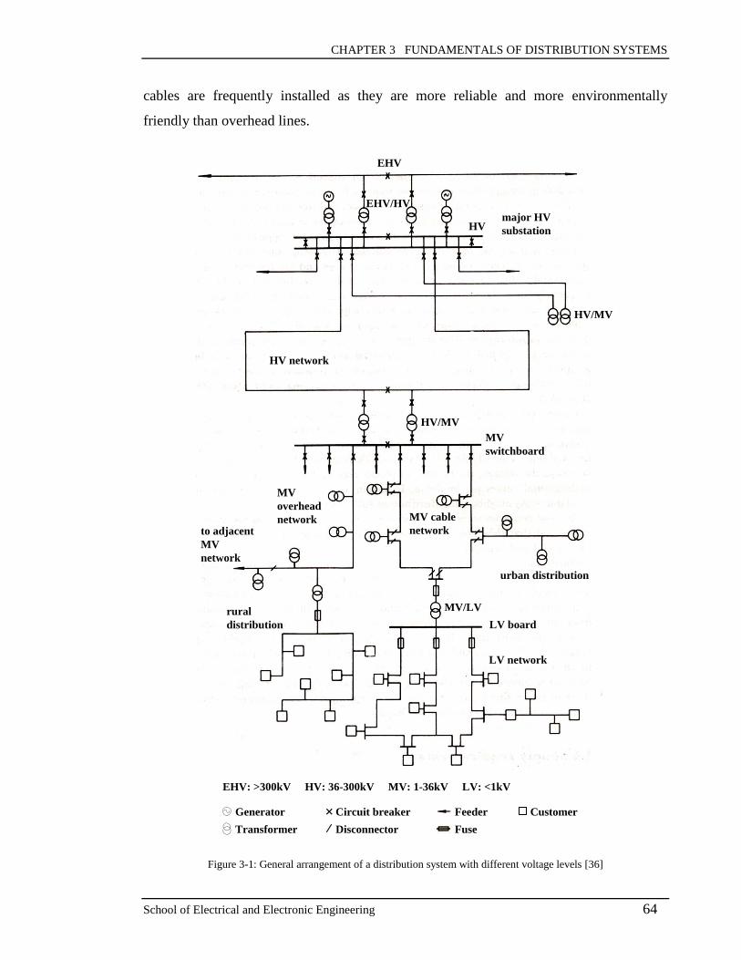
CHAPTER 3 FUNDAMENTALS OF DISTRIBUTION SYSTEMS
School of Electrical and Electronic Engineering 64
cables are frequently installed as they are more reliable and more environmentally
friendly than overhead lines.
EHV
EHV/HV
HVmajor HV
substation
HV/MV
HV network
HV/MV
MV
switchboard
MV cable
network
MV
overhead
networkto adjacent
MV
network
urban distribution
rural
distribution
MV/LV
LV board
LV network
×Generator
Transformer
Circuit breaker
Disconnector
Feeder
Fuse
Customer
EHV: >300kV HV: 36-300kV MV: 1-36kV LV: <1kV
Figure 3-1: General arrangement of a distribution system with different voltage levels [36]

CHAPTER 3 FUNDAMENTALS OF DISTRIBUTION SYSTEMS
School of Electrical and Electronic Engineering 65
Figure 3-1 only indicates a general distribution system arrangement as the design practice
varies from countries to countries. In the UK, the transmission system operates at the
EHV levels with 275kV and 400kV. The voltages are transformed down to 132kV at the
Grid Supply Points (GSPs), where distribution networks are connected to the
transmission system. The distribution HV networks usually operate at 132kV and 33kV.
The HV/MV substation shown in Figure 3-1 is often known as the primary substation,
which converts the voltage from 33kV to 11kV or 6.6kV. For the UK practice, the
primary substation transformers normally operate in parallel, and each has an OLTC
equipped to regulate voltages. The details about tap changer mechanisms and the load
flow modelling of the transformer with tap stagger are discussed in the following sections.
3.3 Voltage Regulation
One of the most important constraints for distribution system design is the voltage level
at the load connection point. The voltage drops on lines or cables may cause voltage
violations if without appropriate compensation. As mentioned in the literature reviews,
voltage control can be accomplished by managing the production and absorption of
reactive power in the system. The relationship between voltage and reactive power is
described in this section.
3.3.1 Voltage drop calculations
Considering a line segment having an impedance R + jX (as shown in Figure 3-2), the
voltage drop due to the line impedance can be expressed as:
∆𝑉 = 𝑉1 − 𝑉2 = (𝑅 + 𝑗𝑋) ∙ 𝐼 = (𝑅 + 𝑗𝑋) (𝑃 − 𝑗𝑄
𝑉1) =
𝑅𝑃 + 𝑋𝑄
𝑉1+ 𝑗
𝑋𝑃 − 𝑅𝑄
𝑉1
= ∆𝑉𝑟 + 𝑗 ∙ ∆𝑉𝑖
(3-1)
where V1 is the voltage at the sending end, V2 is the voltage at the receiving end (or load
centre), I denotes the current through the line impedance, P denotes the active power

CHAPTER 3 FUNDAMENTALS OF DISTRIBUTION SYSTEMS
School of Electrical and Electronic Engineering 66
transmitted out of the sending end and Q for the reactive power. ∆Vr is the real part of ∆V
and ∆Vi is the imaginary component that reflects the angle between V1 and V2.
R + jX
V1 V2
IP + jQ
Figure 3-2: Single-phase equivalent circuit of a line segment in distribution system
For a distribution circuit under normal conditions, ∆Vi is usually neglected as the angle
between V1 and V2 is small [10], [16]. Therefore, the voltage drop ∆V can be simplified as:
∆𝑉 ≈𝑅𝑃 + 𝑋𝑄
𝑉1 (3-2)
According to the equation above, the voltage deviation is related to the power flow (P
and Q) on the line. The power flow predominantly depends on the system load. When the
demand is high, large power flow through the line will lead to a significant voltage drop.
For reduced voltage drops, VAr compensation devices can be installed to provide reactive
power locally, resulting in less reactive power transmitted on the line. Note that if large P
(or Q) flows in the opposite direction, the sign of ∆V may change to negative, which
implies the voltage at the receiving end is greater than the sending end voltage. This
scenario explains the reason why the voltage at the DG connection point increases.
3.3.2 Allowable voltage variations
The distribution system voltage regulation aims to maintain a stable voltage at the
consumer terminals and to control the voltage variation at an acceptable level. In the UK,
the steady state line-line voltage of the system operating at 132kV or above should be
maintained within ±10% of the rated voltage, and ±6% range for the system between 1kV
and 132kV [15]. In terms of the system above 50V and below 1kV, voltage is only

CHAPTER 3 FUNDAMENTALS OF DISTRIBUTION SYSTEMS
School of Electrical and Electronic Engineering 67
permitted with variation between +10% and -6% of the nominal voltage. These
requirements need to be satisfied with at least 95% of the 10-minute mean RMS values of
the supply voltage during a week [116].
3.4 Transformer with On-load Tap Changer
Power transformers equipped with OLTCs have been the main components of electrical
networks for decades. The OLTC provides voltage magnitude regulation and/or phase
shifting by changing the transformer turns ratio under load without interruption. To alter
the transformer turns ratio, the OLTC adds turns to or subtracts turns from either the
primary or the secondary winding. The details of the tap changer mechanisms and the
load flow modelling of a transformer with OLTC are described in this section.
3.4.1 Tap changer mechanisms
Figure 3-3 illustrates the principle winding arrangement for a three-phase regulating
transformer [117]. The OLTC is located at the high-voltage winding with Y connection.
Figure 3-3: Principle winding arrangement of a regulating transformer in Y-∆ connection [117]
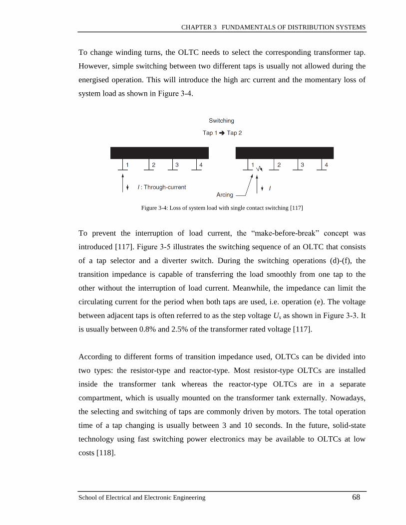
CHAPTER 3 FUNDAMENTALS OF DISTRIBUTION SYSTEMS
School of Electrical and Electronic Engineering 68
To change winding turns, the OLTC needs to select the corresponding transformer tap.
However, simple switching between two different taps is usually not allowed during the
energised operation. This will introduce the high arc current and the momentary loss of
system load as shown in Figure 3-4.
Figure 3-4: Loss of system load with single contact switching [117]
To prevent the interruption of load current, the “make-before-break” concept was
introduced [117]. Figure 3-5 illustrates the switching sequence of an OLTC that consists
of a tap selector and a diverter switch. During the switching operations (d)-(f), the
transition impedance is capable of transferring the load smoothly from one tap to the
other without the interruption of load current. Meanwhile, the impedance can limit the
circulating current for the period when both taps are used, i.e. operation (e). The voltage
between adjacent taps is often referred to as the step voltage Us as shown in Figure 3-3. It
is usually between 0.8% and 2.5% of the transformer rated voltage [117].
According to different forms of transition impedance used, OLTCs can be divided into
two types: the resistor-type and reactor-type. Most resistor-type OLTCs are installed
inside the transformer tank whereas the reactor-type OLTCs are in a separate
compartment, which is usually mounted on the transformer tank externally. Nowadays,
the selecting and switching of taps are commonly driven by motors. The total operation
time of a tap changing is usually between 3 and 10 seconds. In the future, solid-state
technology using fast switching power electronics may be available to OLTCs at low
costs [118].
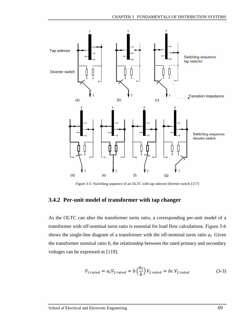
CHAPTER 3 FUNDAMENTALS OF DISTRIBUTION SYSTEMS
School of Electrical and Electronic Engineering 69
Transition impedance
Tap selector
Diverter switch
Figure 3-5: Switching sequence of an OLTC with tap selector-diverter switch [117]
3.4.2 Per-unit model of transformer with tap changer
As the OLTC can alter the transformer turns ratio, a corresponding per-unit model of a
transformer with off-nominal turns ratio is essential for load flow calculations. Figure 3-6
shows the single-line diagram of a transformer with the off-nominal turns ratio at. Given
the transformer nominal ratio b, the relationship between the rated primary and secondary
voltages can be expressed as [119]:
𝑉1 𝑟𝑎𝑡𝑒𝑑 = 𝑎𝑡𝑉2 𝑟𝑎𝑡𝑒𝑑 = 𝑏 (𝑎𝑡
𝑏)𝑉2 𝑟𝑎𝑡𝑒𝑑 = 𝑏𝑐 𝑉2 𝑟𝑎𝑡𝑒𝑑 (3-3)
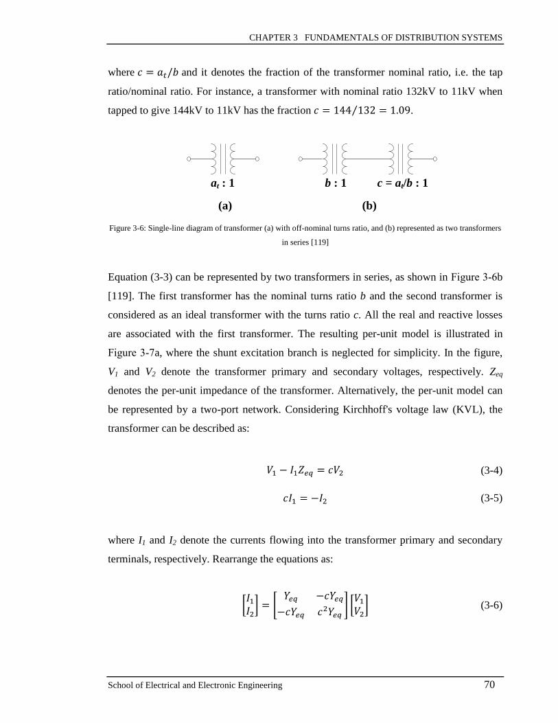
CHAPTER 3 FUNDAMENTALS OF DISTRIBUTION SYSTEMS
School of Electrical and Electronic Engineering 70
where 𝑐 = 𝑎𝑡/𝑏 and it denotes the fraction of the transformer nominal ratio, i.e. the tap
ratio/nominal ratio. For instance, a transformer with nominal ratio 132kV to 11kV when
tapped to give 144kV to 11kV has the fraction 𝑐 = 144 132⁄ = 1.09.
at : 1 b : 1 c = at/b : 1
(a) (b)
Figure 3-6: Single-line diagram of transformer (a) with off-nominal turns ratio, and (b) represented as two transformers
in series [119]
Equation (3-3) can be represented by two transformers in series, as shown in Figure 3-6b
[119]. The first transformer has the nominal turns ratio b and the second transformer is
considered as an ideal transformer with the turns ratio c. All the real and reactive losses
are associated with the first transformer. The resulting per-unit model is illustrated in
Figure 3-7a, where the shunt excitation branch is neglected for simplicity. In the figure,
V1 and V2 denote the transformer primary and secondary voltages, respectively. Zeq
denotes the per-unit impedance of the transformer. Alternatively, the per-unit model can
be represented by a two-port network. Considering Kirchhoff's voltage law (KVL), the
transformer can be described as:
𝑉1 − 𝐼1𝑍𝑒𝑞 = 𝑐𝑉2 (3-4)
𝑐𝐼1 = −𝐼2 (3-5)
where I1 and I2 denote the currents flowing into the transformer primary and secondary
terminals, respectively. Rearrange the equations as:
[𝐼1𝐼2
] = [𝑌𝑒𝑞 −𝑐𝑌𝑒𝑞
−𝑐𝑌𝑒𝑞 𝑐2𝑌𝑒𝑞] [
𝑉1
𝑉2] (3-6)
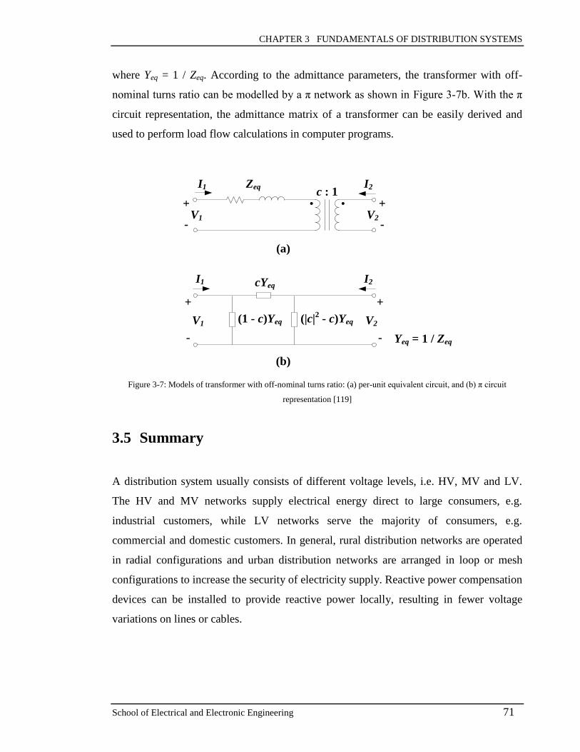
CHAPTER 3 FUNDAMENTALS OF DISTRIBUTION SYSTEMS
School of Electrical and Electronic Engineering 71
where Yeq = 1 / Zeq. According to the admittance parameters, the transformer with off-
nominal turns ratio can be modelled by a π network as shown in Figure 3-7b. With the π
circuit representation, the admittance matrix of a transformer can be easily derived and
used to perform load flow calculations in computer programs.
(a)
(b)
+
-V1
I1 Zeqc : 1
I2
+
-V2
+
-
V1
I1 I2
+
-
V2
cYeq
(1 - c)Yeq (|c|2 - c)Yeq
Yeq = 1 / Zeq
Figure 3-7: Models of transformer with off-nominal turns ratio: (a) per-unit equivalent circuit, and (b) π circuit
representation [119]
3.5 Summary
A distribution system usually consists of different voltage levels, i.e. HV, MV and LV.
The HV and MV networks supply electrical energy direct to large consumers, e.g.
industrial customers, while LV networks serve the majority of consumers, e.g.
commercial and domestic customers. In general, rural distribution networks are operated
in radial configurations and urban distribution networks are arranged in loop or mesh
configurations to increase the security of electricity supply. Reactive power compensation
devices can be installed to provide reactive power locally, resulting in fewer voltage
variations on lines or cables.

CHAPTER 3 FUNDAMENTALS OF DISTRIBUTION SYSTEMS
School of Electrical and Electronic Engineering 72
The switching mechanism and sequence of a typical OLTC have been described. The
“make-before-break” concept has been widely used in the OLTC designs to prevent the
interruption of load current. As the OLTC can alter the transformer turns ratio, a
corresponding per-unit model of a transformer with off-nominal turns ratio has been
derived. The π circuit representation of a transformer with tap changer can be easily
processed by the computer program to perform load flow calculations.

CHAPTER 4 TAP STAGGER FOR REACTIVE POWER SUPPORT
School of Electrical and Electronic Engineering 73
CHAPTER 4
4 TAP STAGGER FOR REACTIVE POWER SUPPORT
4.1 Introduction
With the integration of large-scale intermittent renewable generation, the transmission
voltage problem has become more dynamic and may occur in different time periods or
different regions. The associated costs will be high if numbers of devices need to be
placed at various locations in the system. In addition, the permanent installation of VAr
compensators may not be cost-effective for temporary voltage issues. Therefore, this
chapter proposes an alternative method, which utilises existing distribution parallel
transformers, to provide reactive power absorption services for transmission systems
during periods of low demand. The operation of the parallel transformers in small
different tap positions, i.e. with staggered taps, can provide a means of absorbing reactive
power. The aggregated VAr absorption from many pairs of parallel transformers could be
used to mitigate the high voltages in the upstream network. This chapter first presents the
structure of the proposed VAr support method using tap stagger. The mathematical
principles of the tap staggering operation are then discussed. Following this, an optimal
control approach for the tap stagger is proposed and considers the minimisation of the
introduced power losses and tap switching operations.
4.2 Proposed Distribution Network VAr Support Method with
Tap Stagger
The proposed method of utilising the parallel transformers in a distribution network to
provide VAr support is illustrated in Figure 4-1. The distribution network is connected to
the transmission system at the GSP. The distribution system has ‘N” number of primary
substations located throughout its high voltage network. At each primary substation, two
parallel transformers (e.g. 33/11 kV in the UK) usually operate together, and both have

CHAPTER 4 TAP STAGGER FOR REACTIVE POWER SUPPORT
School of Electrical and Electronic Engineering 74
on-load tap changers (OLTCs) installed, which allow real-time control. Therefore, in this
research work, the proposed tap staggering method is applied to the primary substations.
However, conceptually the tap staggering technique may be adopted at different voltage
levels where there are transformers operating in parallel.
Distribution
Network
Network states
Vi, TAPi
OLTC tap changing
commands
Qrequired
Qrequired : reactive power absorption requirement
∆Q : extra reactive power absorption by tap stagger
L1, … LN : network loads
...
L1
LN
Transmission
System
Grid Supply
Point
DMS
Tap Stagger
Optimal Control
Energy Management
System
(EMS)
Communication
Network
Network
Control Centre
∆Q
: power flow
: control or measurement signal
Figure 4-1: Proposed reactive power absorption service provided by distribution network using tap stagger
When the transmission system needs extra reactive power absorption during periods of
low demand, the Energy Management System (EMS) may send a specific VAr
requirement (Qrequired) to the Distribution Management System (DMS). The Tap Stagger
Optimal Control system embedded in the DMS will then issue tap staggering commands.
The optimal control system determines how many parallel transformers will be used, with
the objectives of minimising the introduced power losses and the number of tap switching
operations. The optimisation is based on the measured network states, such as load level,
voltage Vi and transformer tap position TAPi. The calculated control signals will be sent
to the appropriate primary substations via the communication network, and they will be
received by the remote terminal units (RTUs), which interface with the AVC relays.
According to the tap staggering commands, the AVC relays will instruct the OLTCs of
parallel transformers to tap apart. The proposed method may be considered as a demand

CHAPTER 4 TAP STAGGER FOR REACTIVE POWER SUPPORT
School of Electrical and Electronic Engineering 75
response tool that assists the transmission system in managing reactive power flow for
some temporary or contingency periods.
Based on Figure 4-1, this research project concentrates on the development of the tap
stagger optimal control method as well as the analyses of the tap staggering impacts on
the transmission system. The EMS and communication network are not modelled as it is
assumed that the VAr absorption requirement and the distribution network states are
known in advance. However, for real-time application, the communication plays an
essential role in the successful implementation of the proposed method.
4.3 Tap Stagger Mathematic Principles
At modern electric substations, it is common to see the operation of two or more
transformers in parallel. This practice reduces the load carried by each transformer and
improves the security of the electricity supply. The tap changer of each parallel
transformer is normally maintained at the same position to reduce the circulating current
between the transformers [21], [120]. However, some substations may need to operate the
parallel transformers with offset tap positions, and then a circulation of reactive power
occurs between the transformers, resulting in a net absorption of reactive power. This
operating mode is known as ‘tap stagger’ and is occasionally applied to transmission
substation transformers to introduce inductive loading onto the system [37], [121] and
[122].
To explore the potential benefit of utilising distribution networks to support transmission
system VAr management, this research project focuses on the application of the tap
staggering method at the parallel transformers in distribution networks. The working
principles of the proposed tap staggering technique are described in this section.
4.3.1 Parallel operation of two transformers
Although multiple transformers can be used for parallel operation, this research study
concentrates on the scenario when two transformers are connected in parallel, which is

CHAPTER 4 TAP STAGGER FOR REACTIVE POWER SUPPORT
School of Electrical and Electronic Engineering 76
the typical arrangement for the UK primary substation transformers. Figure 4-2 shows the
single-line diagram of two three-phase transformers arranged in parallel.
As shown in the figure, both the primary and secondary windings of the two transformers
are connected to the same set of primary and secondary busbars, respectively. Therefore,
the two parallel transformers have the same terminal voltages at the primary and
secondary sides. Note that the primary winding of each transformer is equipped with an
OLTC. If the two parallel transformers have the same impedances and both tap changers
are maintained at the same positions, the power flow through one transformer will be
identical to the other.
Source
Load (PL1, QL1)
T1 T2
Pin1, Qin1 Pin2, Qin2
PL2, QL2
Primary busbar
Secondary busbar
Pout1, Qout1 Pout2, Qout2
CB
CB
Figure 4-2: Single-line diagram of two parallel transformers
where,
T1 and T2 Two parallel transformers with OLTCs
Pin1, Qin1, Pin2 and Qin2 Active and reactive power flowing into each transformer
Pout1, Qout1, Pout2 and Qout2 Active and reactive power flowing out of each transformer
PL1, QL1, PL2 and QL2 Loads connected to the secondary (or LV) busbar
CB Circuit breaker
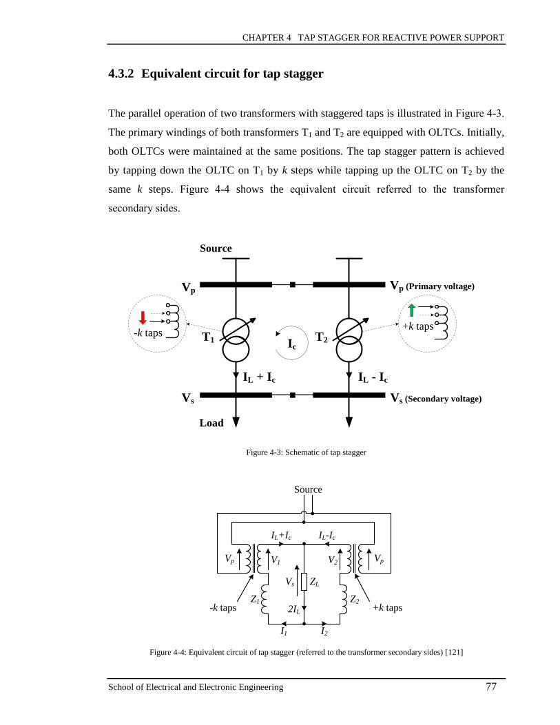
CHAPTER 4 TAP STAGGER FOR REACTIVE POWER SUPPORT
School of Electrical and Electronic Engineering 77
4.3.2 Equivalent circuit for tap stagger
The parallel operation of two transformers with staggered taps is illustrated in Figure 4-3.
The primary windings of both transformers T1 and T2 are equipped with OLTCs. Initially,
both OLTCs were maintained at the same positions. The tap stagger pattern is achieved
by tapping down the OLTC on T1 by k steps while tapping up the OLTC on T2 by the
same k steps. Figure 4-4 shows the equivalent circuit referred to the transformer
secondary sides.
Source
T1 T2
Vs (Secondary voltage)
IL + Ic IL - Ic
Ic
Load
-k taps
Vp
Vs
+k taps
Vp (Primary voltage)
Figure 4-3: Schematic of tap stagger
ZL
Z2Z1
2IL
IL+Ic IL-Ic
V1 V2
Vs
Vp Vp
I1 I2
Source
-k taps +k taps
Figure 4-4: Equivalent circuit of tap stagger (referred to the transformer secondary sides) [121]
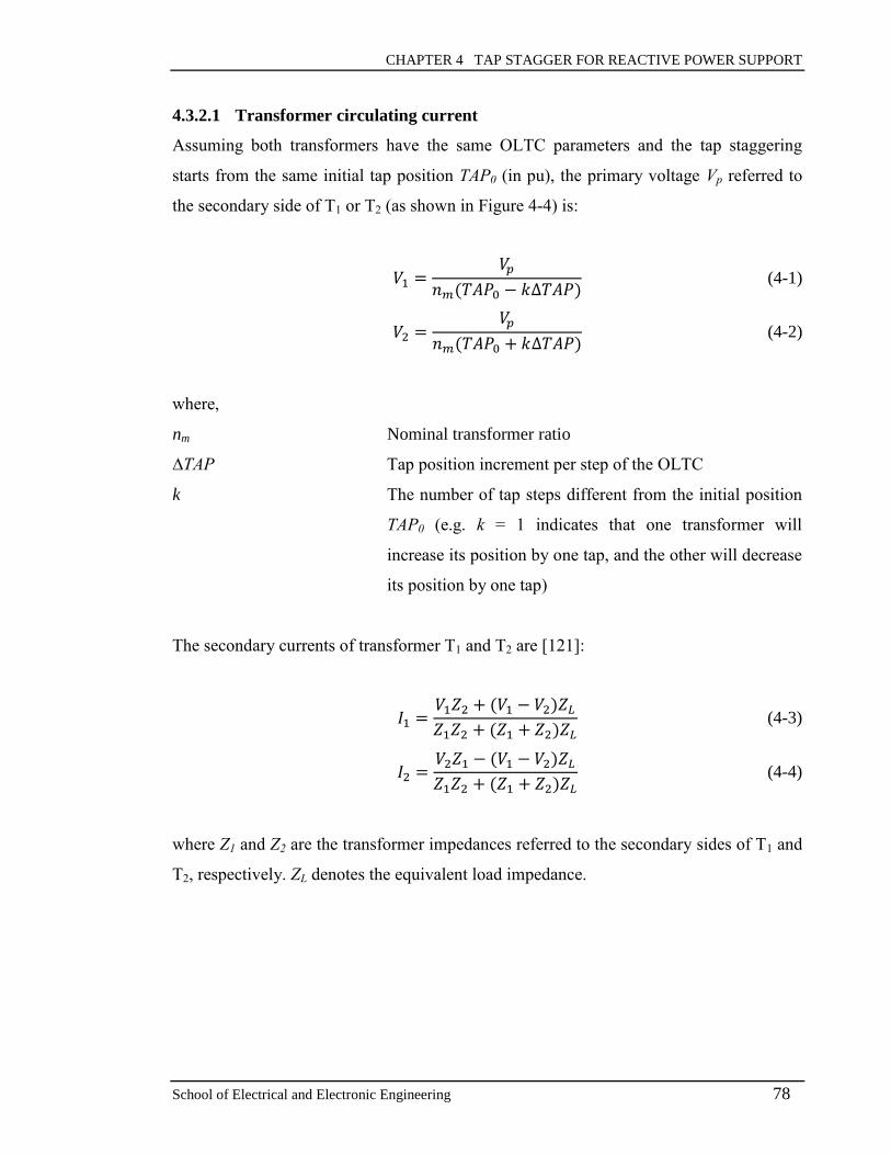
CHAPTER 4 TAP STAGGER FOR REACTIVE POWER SUPPORT
School of Electrical and Electronic Engineering 78
4.3.2.1 Transformer circulating current
Assuming both transformers have the same OLTC parameters and the tap staggering
starts from the same initial tap position TAP0 (in pu), the primary voltage Vp referred to
the secondary side of T1 or T2 (as shown in Figure 4-4) is:
𝑉1 =𝑉𝑝
𝑛𝑚(𝑇𝐴𝑃0 − 𝑘∆𝑇𝐴𝑃) (4-1)
𝑉2 =𝑉𝑝
𝑛𝑚(𝑇𝐴𝑃0 + 𝑘∆𝑇𝐴𝑃) (4-2)
where,
nm Nominal transformer ratio
∆TAP Tap position increment per step of the OLTC
k The number of tap steps different from the initial position
TAP0 (e.g. k = 1 indicates that one transformer will
increase its position by one tap, and the other will decrease
its position by one tap)
The secondary currents of transformer T1 and T2 are [121]:
𝐼1 =𝑉1𝑍2 + (𝑉1 − 𝑉2)𝑍𝐿
𝑍1𝑍2 + (𝑍1 + 𝑍2)𝑍𝐿 (4-3)
𝐼2 =𝑉2𝑍1 − (𝑉1 − 𝑉2)𝑍𝐿
𝑍1𝑍2 + (𝑍1 + 𝑍2)𝑍𝐿 (4-4)
where Z1 and Z2 are the transformer impedances referred to the secondary sides of T1 and
T2, respectively. ZL denotes the equivalent load impedance.
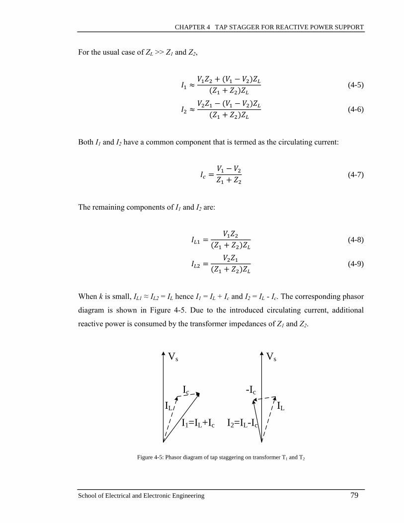
CHAPTER 4 TAP STAGGER FOR REACTIVE POWER SUPPORT
School of Electrical and Electronic Engineering 79
For the usual case of ZL >> Z1 and Z2,
𝐼1 ≈𝑉1𝑍2 + (𝑉1 − 𝑉2)𝑍𝐿
(𝑍1 + 𝑍2)𝑍𝐿 (4-5)
𝐼2 ≈𝑉2𝑍1 − (𝑉1 − 𝑉2)𝑍𝐿
(𝑍1 + 𝑍2)𝑍𝐿 (4-6)
Both I1 and I2 have a common component that is termed as the circulating current:
𝐼𝑐 =𝑉1 − 𝑉2
𝑍1 + 𝑍2 (4-7)
The remaining components of I1 and I2 are:
𝐼𝐿1 =𝑉1𝑍2
(𝑍1 + 𝑍2)𝑍𝐿 (4-8)
𝐼𝐿2 =𝑉2𝑍1
(𝑍1 + 𝑍2)𝑍𝐿 (4-9)
When k is small, IL1 ≈ IL2 = IL hence I1 = IL + Ic and I2 = IL - Ic. The corresponding phasor
diagram is shown in Figure 4-5. Due to the introduced circulating current, additional
reactive power is consumed by the transformer impedances of Z1 and Z2.
Vs
IL
Ic
I1=IL+Ic
Vs
IL
-Ic
I2=IL-Ic
Figure 4-5: Phasor diagram of tap staggering on transformer T1 and T2
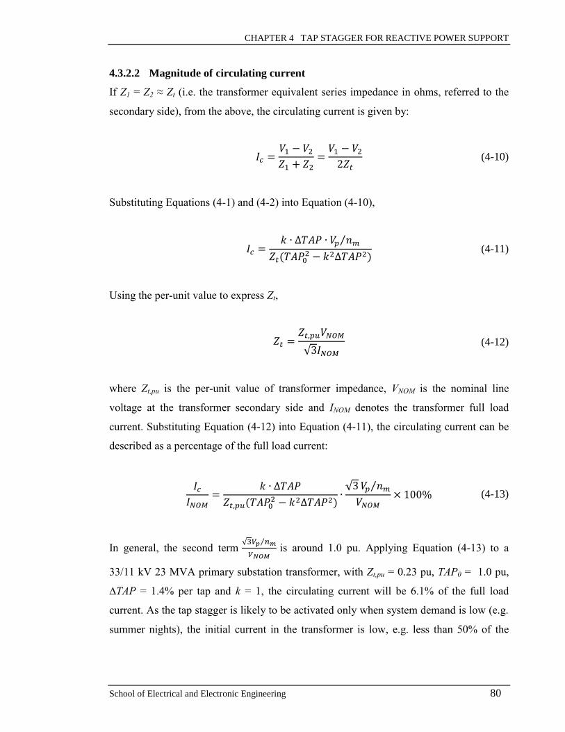
CHAPTER 4 TAP STAGGER FOR REACTIVE POWER SUPPORT
School of Electrical and Electronic Engineering 80
4.3.2.2 Magnitude of circulating current
If Z1 = Z2 ≈ Zt (i.e. the transformer equivalent series impedance in ohms, referred to the
secondary side), from the above, the circulating current is given by:
𝐼𝑐 =𝑉1 − 𝑉2
𝑍1 + 𝑍2=
𝑉1 − 𝑉2
2𝑍𝑡 (4-10)
Substituting Equations (4-1) and (4-2) into Equation (4-10),
𝐼𝑐 =𝑘 ∙ ∆𝑇𝐴𝑃 ∙ 𝑉𝑝 𝑛𝑚⁄
𝑍𝑡(𝑇𝐴𝑃02 − 𝑘2∆𝑇𝐴𝑃2)
(4-11)
Using the per-unit value to express Zt,
𝑍𝑡 =𝑍𝑡,𝑝𝑢𝑉𝑁𝑂𝑀
√3𝐼𝑁𝑂𝑀
(4-12)
where Zt,pu is the per-unit value of transformer impedance, VNOM is the nominal line
voltage at the transformer secondary side and INOM denotes the transformer full load
current. Substituting Equation (4-12) into Equation (4-11), the circulating current can be
described as a percentage of the full load current:
𝐼𝑐
𝐼𝑁𝑂𝑀=
𝑘 ∙ ∆𝑇𝐴𝑃
𝑍𝑡,𝑝𝑢(𝑇𝐴𝑃02 − 𝑘2∆𝑇𝐴𝑃2)
∙√3𝑉𝑝 𝑛𝑚⁄
𝑉𝑁𝑂𝑀× 100% (4-13)
In general, the second term √3𝑉𝑝 𝑛𝑚⁄
𝑉𝑁𝑂𝑀 is around 1.0 pu. Applying Equation (4-13) to a
33/11 kV 23 MVA primary substation transformer, with Zt,pu = 0.23 pu, TAP0 = 1.0 pu,
∆TAP = 1.4% per tap and k = 1, the circulating current will be 6.1% of the full load
current. As the tap stagger is likely to be activated only when system demand is low (e.g.
summer nights), the initial current in the transformer is low, e.g. less than 50% of the

CHAPTER 4 TAP STAGGER FOR REACTIVE POWER SUPPORT
School of Electrical and Electronic Engineering 81
peak load. Therefore, the use of the tap staggering technique is practicable, depending on
the transformer capacity.
4.3.2.3 Reactive power absorption & active power loss due to tap stagger
Based on Equation (4-11), the additional reactive power consumption due to the
circulating current Ic can be derived as:
∆𝑄𝑐 = 2𝐼𝑐2𝑋𝑡 = 2
𝑋𝑡(𝑘 ∙ ∆𝑇𝐴𝑃 ∙ 𝑉𝑝 𝑛𝑚⁄ )2
𝑍𝑡2(𝑇𝐴𝑃0
2 − 𝑘2∆𝑇𝐴𝑃2)2 (4-14)
where Xt is the transformer leakage reactance. Let Zt = Rt + jXt, with Rt representing the
winding resistance.
From the equation above, the VAr absorption introduced by circulating current will
increase with the transformer primary voltage Vp as well as the staggered taps k. The
aggregated VAr absorption seen at the GSP will be the sum of ∆Qc from each substation,
plus the additional VAr transmission loss from the transmission supply point down to the
primary substations. The additional transformer power loss due to the tap stagger can also
be described as:
∆𝑃𝑐 = 2𝐼𝑐2𝑅𝑡 = 2
𝑅𝑡(𝑘 ∙ ∆𝑇𝐴𝑃 ∙ 𝑉𝑝 𝑛𝑚⁄ )2
𝑍𝑡2(𝑇𝐴𝑃0
2 − 𝑘2∆𝑇𝐴𝑃2)2 (4-15)
In general, for large power transformers rated more than 500 kVA, the winding
resistances are much smaller than the leakage reactances [119], hence ∆Pc << ∆Qc. The
comparison studies between the reactive power absorption and real power loss due to tap
stagger are given in Chapter 5.

CHAPTER 4 TAP STAGGER FOR REACTIVE POWER SUPPORT
School of Electrical and Electronic Engineering 82
4.3.2.4 Voltage of downstream network
According to the equivalent circuit shown in Figure 4-4, the transformer secondary
voltage can be derived as:
𝑉𝑠 = (𝐼1 + 𝐼2)𝑍𝐿 =𝑉1 + 𝑉2
2 (4-16)
Substituting Equations (4-1) and (4-2) into Equation (4-16),
𝑉𝑠 =𝑉𝑝
𝑛𝑚(𝑇𝐴𝑃0 − 𝑘2∆𝑇𝐴𝑃2 𝑇𝐴𝑃0⁄ ) (4-17)
Figure 4-6: Transformer secondary voltage with different staggered taps (with ∆TAP = 1.43% and TAP0 = 0.9714 pu)
The ∆TAP of an OLTC transformer is typically less than 2%. Therefore, if the primary
voltage Vp stays the same and small staggered taps (i.e. small k) are applied, the
secondary voltage Vs will remain almost constant, leaving the downstream network
voltages and loads unaffected. Figure 4-6 shows an example of the transformer secondary
voltage against the difference in tap positions of two parallel transformers. The secondary
voltage changes less than 0.05% up to 4 tap differences, i.e. k = 2. With the maximum 12
tap differences, the secondary voltage increases by 0.5%. Therefore, the effect of the
proposed tap staggering method on the downstream network voltages is small.
CHAPTER 4 TAP STAGGER FOR REACTIVE POWER SUPPORT
School of Electrical and Electronic Engineering 83
As aforementioned, the difference in tap positions should only be allowed within a small
range (e.g. 2 taps up for one transformer and 2 taps down for the other) in order to
prevent the transformer overheating and to maintain the secondary voltages constant
without affecting the downstream networks. Although each pair of parallel transformers
can only provide a limited VAr absorption, the total amount aggregated from many
transformers may be sufficient to mitigate the reactive power surplus in the transmission
system. Therefore, Chapter 5 will carry out the feasibility studies to investigate and
quantify the VAr absorption capability of distribution networks with tap stagger.
4.4 Tap Stagger Optimal Control
To provide the VAr absorption service, the distribution network operator needs to decide
how many parallel transformers and staggered taps would be used. Consequently, a
control method should be developed to address the VAr dispatch problem. For instance, if
the transmission system requires a specific reactive power to be consumed during periods
of low demand, the tap stagger control will coordinate the available parallel transformers
inside the distribution network to absorb reactive power. In addition, the tap stagger
control will limit the tap position difference between transformers and it will keep the
switching operations of OLTCs as few as possible to reduce the maintenance costs of tap
changers.
Therefore, this section proposes an optimal control approach for the tap stagger. The
objective is to find an optimal dispatch for the OLTC tap positions of parallel
transformers, minimising the active power losses caused as well as the number of tap
switching operations introduced. The transformer tap positions should be arranged in a
way to achieve the VAr absorption required by the transmission system. In addition, the
optimisation is subject to the transformer and OLTC limits. The details of the objective
function and constraints are described as follows.
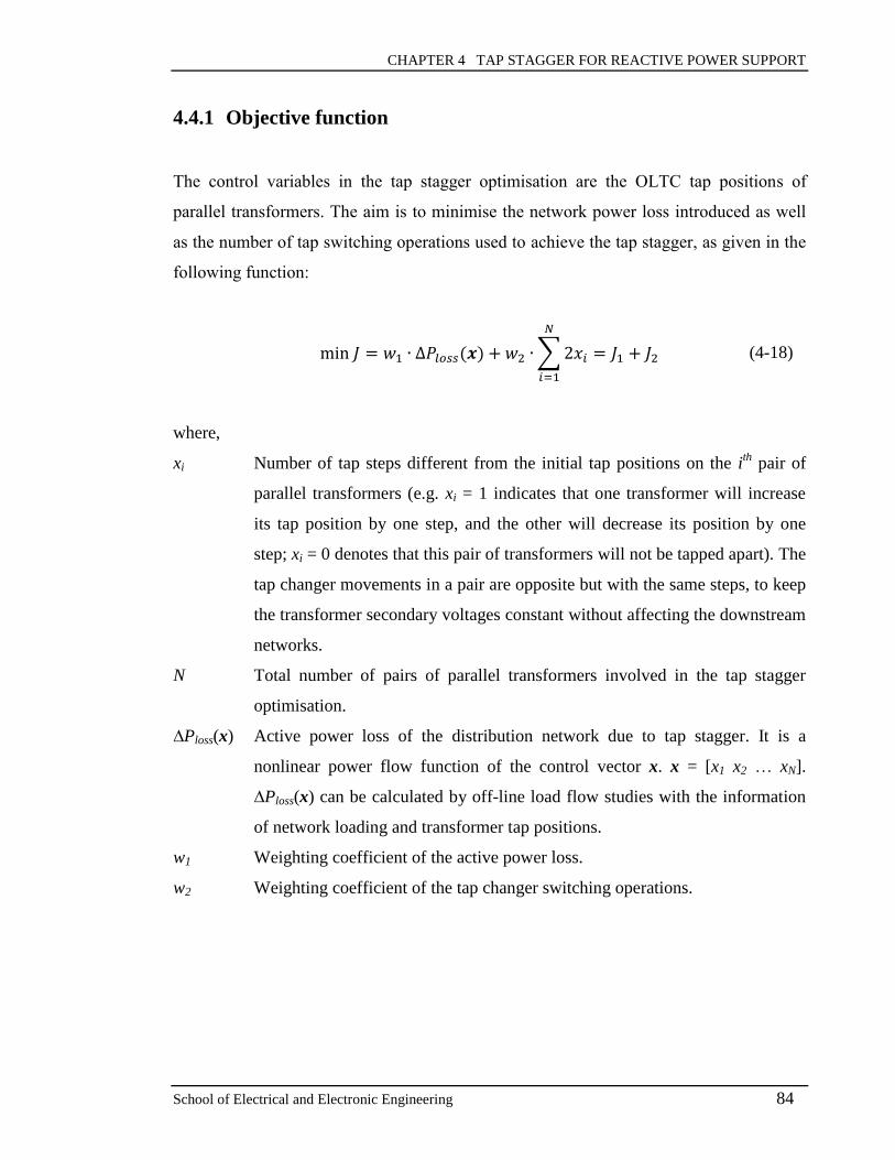
CHAPTER 4 TAP STAGGER FOR REACTIVE POWER SUPPORT
School of Electrical and Electronic Engineering 84
4.4.1 Objective function
The control variables in the tap stagger optimisation are the OLTC tap positions of
parallel transformers. The aim is to minimise the network power loss introduced as well
as the number of tap switching operations used to achieve the tap stagger, as given in the
following function:
min 𝐽 = 𝑤1 ∙ ∆𝑃𝑙𝑜𝑠𝑠(𝒙) + 𝑤2 ∙ ∑2𝑥𝑖
𝑁
𝑖=1
= 𝐽1 + 𝐽2 (4-18)
where,
xi Number of tap steps different from the initial tap positions on the ith
pair of
parallel transformers (e.g. xi = 1 indicates that one transformer will increase
its tap position by one step, and the other will decrease its position by one
step; xi = 0 denotes that this pair of transformers will not be tapped apart). The
tap changer movements in a pair are opposite but with the same steps, to keep
the transformer secondary voltages constant without affecting the downstream
networks.
N Total number of pairs of parallel transformers involved in the tap stagger
optimisation.
∆Ploss(x) Active power loss of the distribution network due to tap stagger. It is a
nonlinear power flow function of the control vector x. x = [x1 x2 … xN].
∆Ploss(x) can be calculated by off-line load flow studies with the information
of network loading and transformer tap positions.
w1 Weighting coefficient of the active power loss.
w2 Weighting coefficient of the tap changer switching operations.
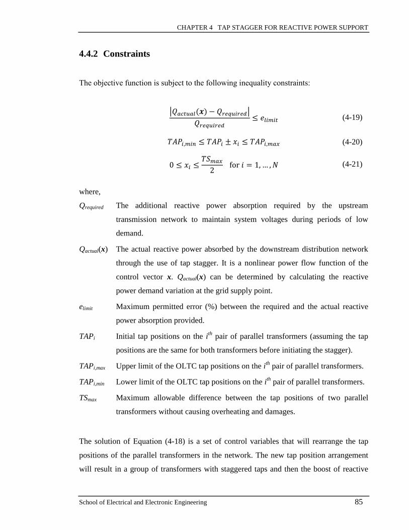
CHAPTER 4 TAP STAGGER FOR REACTIVE POWER SUPPORT
School of Electrical and Electronic Engineering 85
4.4.2 Constraints
The objective function is subject to the following inequality constraints:
|𝑄𝑎𝑐𝑡𝑢𝑎𝑙(𝒙) − 𝑄𝑟𝑒𝑞𝑢𝑖𝑟𝑒𝑑|
𝑄𝑟𝑒𝑞𝑢𝑖𝑟𝑒𝑑≤ 𝑒𝑙𝑖𝑚𝑖𝑡 (4-19)
𝑇𝐴𝑃𝑖,𝑚𝑖𝑛 ≤ 𝑇𝐴𝑃𝑖 ± 𝑥𝑖 ≤ 𝑇𝐴𝑃𝑖,𝑚𝑎𝑥 (4-20)
0 ≤ 𝑥𝑖 ≤𝑇𝑆𝑚𝑎𝑥
2 for 𝑖 = 1, … , 𝑁 (4-21)
where,
Qrequired The additional reactive power absorption required by the upstream
transmission network to maintain system voltages during periods of low
demand.
Qactual(x) The actual reactive power absorbed by the downstream distribution network
through the use of tap stagger. It is a nonlinear power flow function of the
control vector x. Qactual(x) can be determined by calculating the reactive
power demand variation at the grid supply point.
elimit Maximum permitted error (%) between the required and the actual reactive
power absorption provided.
TAPi Initial tap positions on the ith
pair of parallel transformers (assuming the tap
positions are the same for both transformers before initiating the stagger).
TAPi,max Upper limit of the OLTC tap positions on the ith
pair of parallel transformers.
TAPi,min Lower limit of the OLTC tap positions on the ith
pair of parallel transformers.
TSmax Maximum allowable difference between the tap positions of two parallel
transformers without causing overheating and damages.
The solution of Equation (4-18) is a set of control variables that will rearrange the tap
positions of the parallel transformers in the network. The new tap position arrangement
will result in a group of transformers with staggered taps and then the boost of reactive

CHAPTER 4 TAP STAGGER FOR REACTIVE POWER SUPPORT
School of Electrical and Electronic Engineering 86
power consumption. Figure 4-7 illustrates the block diagram of the tap stagger optimal
control. As the control variable xi is treated as a discrete variable and the calculations of
VAr absorption involve nonlinear load flow equations, the tap staggering optimisation
problem is an integer nonlinear programming problem. For this project, the problem has
been solved using the genetic algorithm, the rule-based approach and the Branch-and-
Bound algorithm, respectively. The related solution procedures and result comparisons
are described in Chapters 6 and 7.
……
Qrequired
#1 pair
AVC
relay
AVC
relayRTU
∆Q1
#N pair
AVC
relay
AVC
relayRTU
Distribution Network
Tap Stagger Optimal Control
Transmission Energy
Management System
∆QN
Communication Link
x1
xN
Solution
Algorithm
…
Figure 4-7: Block diagram of the tap stagger optimal control
4.5 Summary
In this chapter, a reactive power control method, utilising the existing parallel
transformers in distribution networks, has been proposed. The operation of the parallel
transformers with staggered taps provides a means of absorbing reactive power, thus
reducing the overvoltages in the upstream transmission system while leaving the
downstream networks unaffected. In this research work, the proposed tap staggering
CHAPTER 4 TAP STAGGER FOR REACTIVE POWER SUPPORT
School of Electrical and Electronic Engineering 87
method is applied to the primary substation transformers, which are equipped with
OLTCs to allow on-line control.
The equivalent circuit of two parallel transformers with staggered taps has been presented.
According to the analysis of the equivalent circuit, the circulating current increases with
the staggered taps. As the tap stagger is likely to be adopted only during periods of low
demand, the initial current in the transformer is low. Therefore, the transformer current
could remain within the limit if the staggered taps are small. In addition, the use of small
staggered taps can keep the transformer secondary voltage almost constant, leaving the
downstream network voltages and loads unaffected.
Furthermore, an optimal control approach for the tap staggering operation has been
proposed. The objective is to find an optimal dispatch for the OLTC tap positions, which
minimises the network loss and the number of switching operations introduced when
providing the VAr absorption. The implementation of the tap stagger control using the
genetic algorithm will be presented in Chapter 6.
CHAPTER 5 NETWORK REACTIVE POWER ABSORPTION CAPABILITY STUDIES
School of Electrical and Electronic Engineering 88
CHAPTER 5
5 NETWORK REACTIVE POWER ABSORPTION
CAPABILITY STUDIES
5.1 Introduction
This chapter presents the feasibility studies of assessing the distribution network reactive
power absorption through the use of the tap staggering technique. Off-line load flow
studies are carried out based on a real UK HV distribution network model. The studies
consist of two parts. The first part aims to investigate the maximum potential VAr
absorption that can be provided with the consideration of OLTC operating limits and
transformer ratings. Both the network reactive power absorption and active power loss
due to the tap stagger are analysed. For the concern of transformer health, the second part
presents a more conservative study by constraining the number of staggered taps. The
details are given as follows.
5.2 Distribution Network Modelling
To investigate the feasibility of using the tap staggering technique, a load flow model of a
real UK HV distribution network has been studied. The model has been provided from
the ‘Customer Load Active System Services (CLASS)’ project, which is funded by the
Office of Gas and Electricity Markets (Ofgem) [123]. The distribution system has been
modelled using the Interactive Power System Analysis (IPSA) software [124]. The
network data and the IPSA model are shown in APPENDIX A. Figure 5-1 illustrates the
basic network components at different voltage levels.
As illustrated in Figure 5-1, the distribution system is configured as a radial network and
the main source is from the grid infeed with 400kV and 275kV voltages. The distribution
network is operated at four different voltage levels, i.e. 132kV, 33kV, 11kV and 6.6kV.
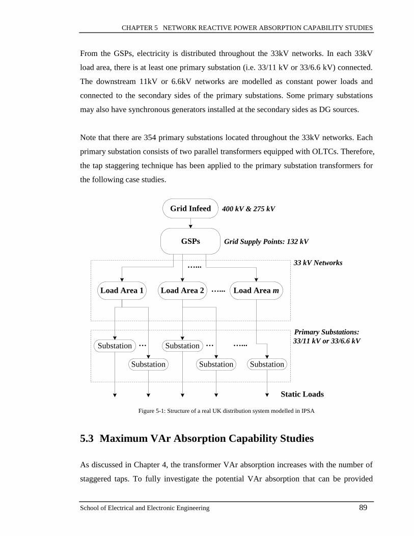
CHAPTER 5 NETWORK REACTIVE POWER ABSORPTION CAPABILITY STUDIES
School of Electrical and Electronic Engineering 89
From the GSPs, electricity is distributed throughout the 33kV networks. In each 33kV
load area, there is at least one primary substation (i.e. 33/11 kV or 33/6.6 kV) connected.
The downstream 11kV or 6.6kV networks are modelled as constant power loads and
connected to the secondary sides of the primary substations. Some primary substations
may also have synchronous generators installed at the secondary sides as DG sources.
Note that there are 354 primary substations located throughout the 33kV networks. Each
primary substation consists of two parallel transformers equipped with OLTCs. Therefore,
the tap staggering technique has been applied to the primary substation transformers for
the following case studies.
Grid Infeed
GSPs Grid Supply Points: 132 kV
Load Area 1
33 kV Networks
Substation
Primary Substations:
33/11 kV or 33/6.6 kVSubstation Substation
Substation
… …...
Static Loads
400 kV & 275 kV
Load Area 2 Load Area m…...
…...
Substation
…
Figure 5-1: Structure of a real UK distribution system modelled in IPSA
5.3 Maximum VAr Absorption Capability Studies
As discussed in Chapter 4, the transformer VAr absorption increases with the number of
staggered taps. To fully investigate the potential VAr absorption that can be provided
CHAPTER 5 NETWORK REACTIVE POWER ABSORPTION CAPABILITY STUDIES
School of Electrical and Electronic Engineering 90
through the use of tap stagger, this section focuses on the studies without setting
permitted limits on the staggered taps. The maximum tap positions that can be tapped
apart will depend on the OLTC operating ranges and transformer ratings. Since there are
large numbers of primary substations in the network (i.e. 354 pairs), it can be time-
consuming to test every pair of transformers. To reduce the complexity, the following
Case 1 has first studied the power flow variations with only one pair of parallel
transformers tapped apart. Then in Case 2, the network has been tested again by
increasing the transformer pairs with tap stagger. The results are used to estimate the
average VAr absorption of the overall system.
5.3.1 Case 1: Reactive power absorption capability of single pair of
parallel transformers
As described before, the tap staggering technique has been applied to the parallel
transformers at the primary substations. For instance, A_t11 and A_t12 are two 33/6.6 kV
transformers configured as shown in Figure 5-2. The parameters of the two transformers
are the same and both OLTCs stay at the same positions. The initial tap position was pre-
calculated by the AVC controller, which maintained the transformer secondary voltage Vs
at the set point 1.0 pu. The controller was then disabled to allow the tap staggering
operation. The simulation started by tapping down the OLTC on A_t11. Meanwhile, the
tap changer on A_t12 was increased by the same steps to keep Vs constant. The simulation
would be stopped if either one transformer reached its tap position limit or the current of
one transformer exceeded the rating. Table 5-1 and Table 5-2 summarise the resulting
reactive and active power flow changes, respectively.
As expected, the total reactive power absorbed by the two transformers is lowest when
both tap positions are the same. Due to the increase in tap step difference, more
circulating currents are produced and then the VAr absorption increases. According to
Table 5-1, the large tap difference (i.e. > 4 staggered taps) has reversed the reactive
power flow of A_t12, resulting in a leading power factor for the transformer. This can be
explained by the phasor diagram in Figure 4-5. Note that during the simulation, the

CHAPTER 5 NETWORK REACTIVE POWER ABSORPTION CAPABILITY STUDIES
School of Electrical and Electronic Engineering 91
transformer secondary voltage stays almost constant, which is consistent with Equation
(4-17). The maximum variation of secondary voltage is 0.48% at the 12 staggered tap
steps.
33kV lines
Static Load
(PL1, QL1)
A_t11 A_t12
Pin1, Qin1 Pin2, Qin2
PL2, QL2
33kV busbar
6.6kV busbar
Pout1, Qout1 Pout2, Qout2
CB
CB
Figure 5-2: Example of two parallel transformers at a primary substation in the IPSA model
where,
CB Circuit breaker
Pin1, Qin1, Pin2 and Qin2 Active and reactive power flowing into each transformer
Pout1, Qout1, Pout2 and Qout2 Active and reactive power flowing out of each transformer
PL1, QL1, PL2 and QL2 Static loads connected to the secondary busbar,
PL1 = PL2, QL1 = QL2.
Based on Table 5-1, the additional reactive power absorption is plotted against the tap
step difference in Figure 5-3. As shown in the figure, the additional VAr absorption is
zero at the initial point since the same tap positions on both transformers will not create
circulating currents. Figure 5-3 also shows the additional VAr absorption that has been
calculated using Equation (4-14), with TAP0 = 0.9714 pu, ∆TAP = 1.43%, Rt = 0.92% and
Xt = 23%. As can be seen from the figure, the simulation and calculation results match
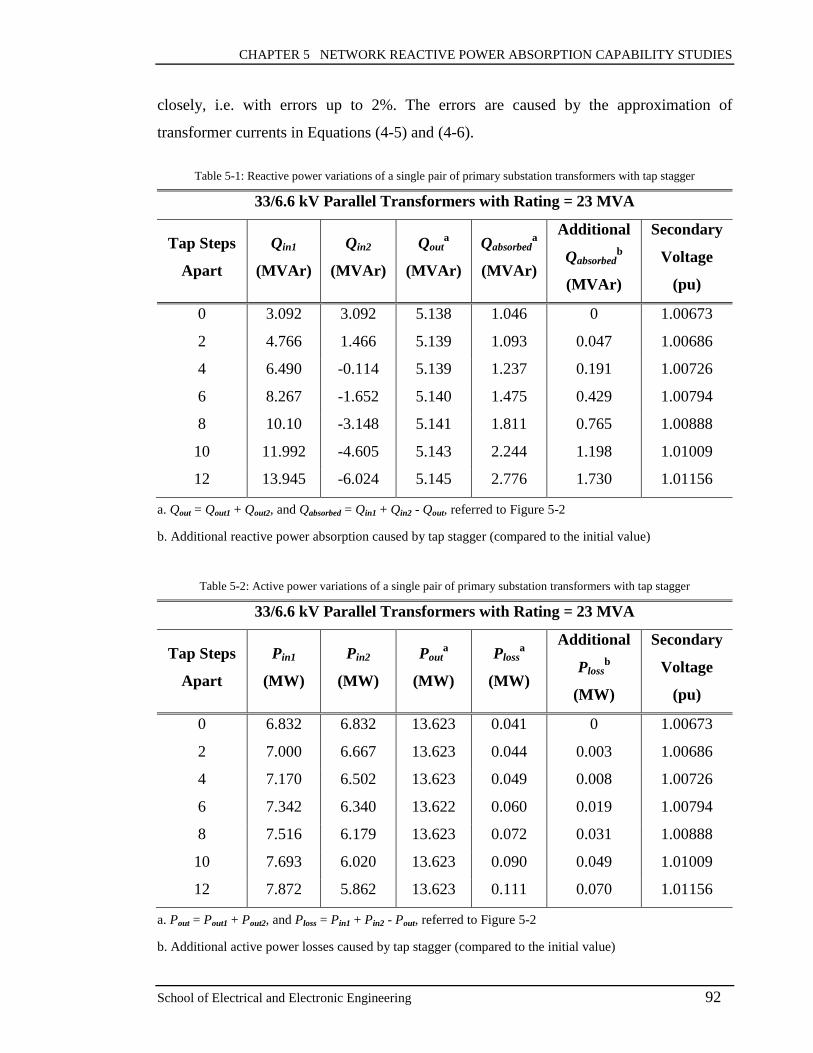
CHAPTER 5 NETWORK REACTIVE POWER ABSORPTION CAPABILITY STUDIES
School of Electrical and Electronic Engineering 92
closely, i.e. with errors up to 2%. The errors are caused by the approximation of
transformer currents in Equations (4-5) and (4-6).
Table 5-1: Reactive power variations of a single pair of primary substation transformers with tap stagger
33/6.6 kV Parallel Transformers with Rating = 23 MVA
Tap Steps
Apart
Qin1
(MVAr)
Qin2
(MVAr)
Qouta
(MVAr)
Qabsorbeda
(MVAr)
Additional
Qabsorbedb
(MVAr)
Secondary
Voltage
(pu)
0 3.092 3.092 5.138 1.046 0 1.00673
2 4.766 1.466 5.139 1.093 0.047 1.00686
4 6.490 -0.114 5.139 1.237 0.191 1.00726
6 8.267 -1.652 5.140 1.475 0.429 1.00794
8 10.10 -3.148 5.141 1.811 0.765 1.00888
10 11.992 -4.605 5.143 2.244 1.198 1.01009
12 13.945 -6.024 5.145 2.776 1.730 1.01156
a. Qout = Qout1 + Qout2, and Qabsorbed = Qin1 + Qin2 - Qout, referred to Figure 5-2
b. Additional reactive power absorption caused by tap stagger (compared to the initial value)
Table 5-2: Active power variations of a single pair of primary substation transformers with tap stagger
33/6.6 kV Parallel Transformers with Rating = 23 MVA
Tap Steps
Apart
Pin1
(MW)
Pin2
(MW)
Pouta
(MW)
Plossa
(MW)
Additional
Plossb
(MW)
Secondary
Voltage
(pu)
0 6.832 6.832 13.623 0.041 0 1.00673
2 7.000 6.667 13.623 0.044 0.003 1.00686
4 7.170 6.502 13.623 0.049 0.008 1.00726
6 7.342 6.340 13.622 0.060 0.019 1.00794
8 7.516 6.179 13.623 0.072 0.031 1.00888
10 7.693 6.020 13.623 0.090 0.049 1.01009
12 7.872 5.862 13.623 0.111 0.070 1.01156
a. Pout = Pout1 + Pout2, and Ploss = Pin1 + Pin2 - Pout, referred to Figure 5-2
b. Additional active power losses caused by tap stagger (compared to the initial value)

CHAPTER 5 NETWORK REACTIVE POWER ABSORPTION CAPABILITY STUDIES
School of Electrical and Electronic Engineering 93
Figure 5-4 indicates the additional active power losses of the transformers from both the
simulation and calculation results. According to the results, the transformer power losses
increase quadratically as the tap step difference increases. However, as transformers are
usually more inductive than resistive, the increase in Ploss (i.e. maximum 0.07 MW) is
small compared to the increment of Qabsorbed (i.e. maximum 1.73 MVAr).
Figure 5-3: Additional reactive power absorption of a pair of parallel transformers with tap stagger
Figure 5-4: Additional active power losses of a pair of parallel transformers with tap stagger
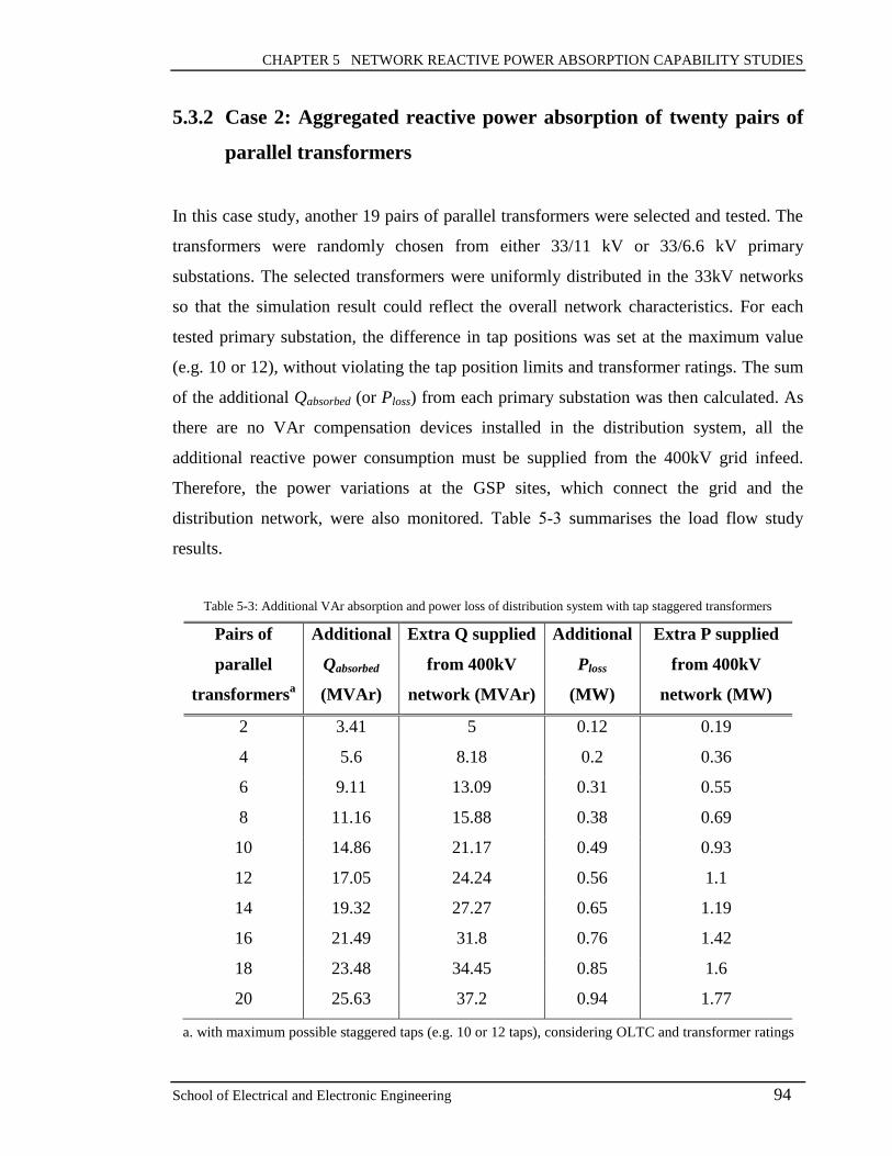
CHAPTER 5 NETWORK REACTIVE POWER ABSORPTION CAPABILITY STUDIES
School of Electrical and Electronic Engineering 94
5.3.2 Case 2: Aggregated reactive power absorption of twenty pairs of
parallel transformers
In this case study, another 19 pairs of parallel transformers were selected and tested. The
transformers were randomly chosen from either 33/11 kV or 33/6.6 kV primary
substations. The selected transformers were uniformly distributed in the 33kV networks
so that the simulation result could reflect the overall network characteristics. For each
tested primary substation, the difference in tap positions was set at the maximum value
(e.g. 10 or 12), without violating the tap position limits and transformer ratings. The sum
of the additional Qabsorbed (or Ploss) from each primary substation was then calculated. As
there are no VAr compensation devices installed in the distribution system, all the
additional reactive power consumption must be supplied from the 400kV grid infeed.
Therefore, the power variations at the GSP sites, which connect the grid and the
distribution network, were also monitored. Table 5-3 summarises the load flow study
results.
Table 5-3: Additional VAr absorption and power loss of distribution system with tap staggered transformers
Pairs of
parallel
transformersa
Additional
Qabsorbed
(MVAr)
Extra Q supplied
from 400kV
network (MVAr)
Additional
Ploss
(MW)
Extra P supplied
from 400kV
network (MW)
2 3.41 5 0.12 0.19
4 5.6 8.18 0.2 0.36
6 9.11 13.09 0.31 0.55
8 11.16 15.88 0.38 0.69
10 14.86 21.17 0.49 0.93
12 17.05 24.24 0.56 1.1
14 19.32 27.27 0.65 1.19
16 21.49 31.8 0.76 1.42
18 23.48 34.45 0.85 1.6
20 25.63 37.2 0.94 1.77
a. with maximum possible staggered taps (e.g. 10 or 12 taps), considering OLTC and transformer ratings
CHAPTER 5 NETWORK REACTIVE POWER ABSORPTION CAPABILITY STUDIES
School of Electrical and Electronic Engineering 95
From Table 5-3, the additional Qabsorbed increases with the number of transformer pairs
using tap stagger. The extra reactive power supplied from the 400kV grid is higher than
the transformer consumption. This is due to the reactive power transmission losses
between the GSPs and primary substations. In Figure 5-5, the additional Q absorptions at
the transformer or the 400kV grid sides are plotted against the transformer pairs.
According to the simulation results of the 20 primary substations, trendlines have also
been produced in Figure 5-5. Due to the radial configuration of the distribution system,
the power flows of primary substations are almost independent of each other. Therefore,
the linear fitting method [125], [126] has been used to estimate the relationship between
the VAr absorption and the number of transformer pairs. The relationship can be
described as:
𝑦 = 𝛽0 + 𝛽1𝑥, 𝑤𝑖𝑡ℎ 𝑅2 ∈ (0, 1) (5-1)
where x denotes the pairs of parallel transformers with tap staggered, and y denotes the
additional reactive power absorption introduced. β0 is the intercept, and β1 is the slope, i.e.
the rate of change in y per unit change in x. R2 is the coefficient of determination, which
indicates how well the measured data fit the estimated trendline [126]. An estimated
model is most accurate when the coefficient is at or near 1. The details of the derivation
of β0, β1 and R2 are given in APPENDIX B.
As shown in Figure 5-5, the relationship between the VAr absorption and the number of
transformers has been estimated as:
𝑦1 = 1.2837𝑥 + 0.9005, with R2 = 0.9939 (5-2)
𝑦2 = 1.8699𝑥 + 1.1445, with R2 = 0.9956 (5-3)
where x denotes the number of transformer pairs (with the maximum possible staggered
taps), y1 and y2 represent the additional VAr absorption seen from the transformer and the
400kV grid sides, respectively. In Equations (5-2) and (5-3), the values of R2 are higher

CHAPTER 5 NETWORK REACTIVE POWER ABSORPTION CAPABILITY STUDIES
School of Electrical and Electronic Engineering 96
than 0.99, which proves the linear estimation is accurate. The slope of the trendline (at
the transformer side) is 1.28, which implies a maximum of 1.28 MVAr can be consumed
by tapping one pair of primary substation transformers apart. Figure 5-5 also indicates a
maximum consumption of 1.87 MVAr/substation at the 400kV grid side (including the
VAr absorption from the 132kV GSPs down to the 33kV primary substations). There are
354 primary substations within the distribution network model to which the tap
staggering technique can be applied. Consequently, the total potential VAr absorption
capability of the overall distribution system would be 662 MVAr.
Figure 5-5: Aggregated Q absorption from 20 pairs of parallel transformers (with maximum staggered taps)
In terms of active power, the additional Ploss at the transformer and 400kV grid sides are
plotted against the transformer pairs in Figure 5-6. The additional power loss due to tap
stagger could be a maximum of 0.088 MW/substation (observed from the 400kV side).
The aggregated loss of the entire distribution network would be 31 MW, corresponding to
about 0.6% of the active power flow in the network. Note that this is the largest power
loss that would be generated when using the maximum available staggered taps. The loss
can be reduced by limiting the tap step difference. A more cautious study with fewer
staggered taps is given in the following case.

CHAPTER 5 NETWORK REACTIVE POWER ABSORPTION CAPABILITY STUDIES
School of Electrical and Electronic Engineering 97
Figure 5-6: Aggregated P losses from 20 pairs of parallel transformers (with maximum staggered taps)
5.4 Conservative VAr Absorption Capability Studies
From the studies in the previous section, an aggregated VAr absorption of 662 MVAr has
been estimated for the overall distribution network. The results have assumed all the
primary substation transformers can be set with the maximum staggered taps (e.g. 10 or
12 taps depending on the OLTC and transformer ratings). However in practice, due to
network demand variations, the initial OLTC position may not be close to the nominal
position, resulting in less headroom for the tap stagger. In addition, a large difference in
tap positions will introduce more transformer losses and may lead to overheating.
Therefore, considering the transformer health and network losses, a more cautious study
of transformers with 4 staggered tap steps (i.e. 2 tap up for one transformer and 2 tap
down for the other) has been carried out in this section. The testing procedure was similar
to Case 2. However, the 20 pairs of primary substation transformers were only allowed to
operate with 4 staggered taps.

CHAPTER 5 NETWORK REACTIVE POWER ABSORPTION CAPABILITY STUDIES
School of Electrical and Electronic Engineering 98
Figure 5-7 illustrates the simulation results. From the figure, an average VAr absorption
of 0.24 MVAr/substation can be observed from the 400kV grid side and the aggregated
VAr consumption of the overall distribution network (with 354 primary substations) will
be 85 MVAr. In general, the additional VAr absorption is expected to be needed during
periods of low demand, e.g. summer nights. Therefore, assuming there are 4 hours per
night over a 90-day period, the total reactive energy absorption would be 30.6 GVArh
(with 4 staggered taps). If other distribution networks connected to the same transmission
system can also participate in the reactive power service, a significant amount of VAr
absorption would be provided to support the transmission system.
Figure 5-7: Aggregated Q absorption from 20 pairs of parallel transformers (with 4 staggered taps)
Figure 5-8 shows the aggregated power loss of the distribution network due to the tap
stagger. In the case of applying 4 staggered taps, the average loss is 0.012 MW/substation
(at the 400kV grid side) and a total loss of 4 MW for the overall distribution system.
Compared with the maximum tap staggering study in Case 2 (see Figure 5-6), the use of 4
staggered taps has reduced the power loss by 87%. Since the tap staggering operation is
likely to be initiated when the network loading becomes low, the small increase in the
network losses may not have significant impacts on the system security. The dynamic
performance of the tap staggering method will be discussed in Chapter 8.

CHAPTER 5 NETWORK REACTIVE POWER ABSORPTION CAPABILITY STUDIES
School of Electrical and Electronic Engineering 99
Figure 5-8: Aggregated P losses from 20 pairs of parallel transformers (with 4 staggered taps)
5.5 Summary
This chapter has presented the feasibility studies in order to assess the VAr absorption
capability of the distribution network through the use of the tap staggering technique.
Off-line load flow studies have been carried out based on a real UK HV distribution
system model. The model consists of the networks from the 132kV GSPs down to the
33kV primary substations. During the simulations, the tap staggering method has been
applied to the parallel transformers at the primary substations.
Case 1 has demonstrated the reactive and real power variations of a single pair of parallel
transformers with tap stagger. From the results, both the VAr absorption and power losses
of the transformers have increased with the number of staggered taps. The results are also
consistent with the theoretical calculation results. In Case 2, 20 pairs of primary
substation transformers have been tested again. Based on the results, the curve fitting
method has been used to estimate the aggregated VAr absorption of the overall
distribution system. According to the estimate, the distribution network can provide a
CHAPTER 5 NETWORK REACTIVE POWER ABSORPTION CAPABILITY STUDIES
School of Electrical and Electronic Engineering 100
total 662 MVAr absorption to the 400kV grid if all the primary substation transformers
are allowed to operate at the maximum staggered taps. However in practice, due to the
variations of network demands, the initial OLTC position may not be at or near the
nominal position, resulting in less headroom for the tap stagger. In addition, the large tap
difference will introduce more losses and may lead to transformer overloading. Therefore,
conservative studies have been carried out considering the transformers with only 4
staggered taps. The results indicate that the aggregated VAr absorption of the distribution
network is 85 MVAr, and the introduced network loss is 4 MW, which corresponds to
0.08% of the active power flow in the network.
The network capability studies in this chapter aim to demonstrate the potential of using
the tap staggering method to provide the VAr absorption service. The results have
confirmed that the distribution network has the potential to support the reactive power
management in the transmission system. If each distribution network can offer a certain
amount of VAr absorption, the transmission system can utilise these inductive VArs to
mitigate the high voltages for some temporary periods. The impacts of the distribution
network VAr absorption on the transmission system will be analysed in Chapter 8.
CHAPTER 6 IMPLEMENTATION OF TAP STAGGER CONTROL USING GA
School of Electrical and Electronic Engineering 101
CHAPTER 6
6 IMPLEMENTATION OF TAP STAGGER CONTROL
USING GA
6.1 Introduction
As discussed in the previous chapter, the employment of tap stagger in distribution
networks has the potential to provide the VAr absorption service and to increase the
utilisation of existing assets. Therefore, this chapter aims to address the issue of how to
provide the VAr absorption service when it is needed. For instance, if the upstream
transmission grid requires a specific reactive power to be consumed during periods of low
demand, the distribution system should be able to decide how many parallel transformers
and staggered taps will be used to meet the requirement. It is also important to keep the
switching operations of OLTCs as few as possible to reduce the maintenance costs of tap
changers.
This chapter presents the implementation of the optimal tap stagger control method
proposed in Chapter 4 (see Figure 4-7). The control objective is to find an optimal
dispatch for the tap positions of the parallel transformers, minimising the active power
losses caused as well as the number of tap switching operations introduced. The solution
algorithm is based on Genetic Algorithm (GA), which can solve mixed-integer nonlinear
programming (MINLP) problems with fast convergence. The details of the
implementation process and testing results are described as follows.
6.2 Network Modelling in OpenDSS
In Chapter 5, an IPSA distribution network model has been provided by the ‘CLASS’
project [123]. The proposed tap stagger optimal control requires the information of the
network states, e.g. load levels, voltages and transformer tap positions. However, the
CHAPTER 6 IMPLEMENTATION OF TAP STAGGER CONTROL USING GA
School of Electrical and Electronic Engineering 102
IPSA model does not provide an interface for an external program to access load flow
results. Therefore, to have communications between the control algorithm and the
network states, the distribution system has been modelled using another power flow
software, i.e. the OpenDSS [127].
The Open Distribution System Simulator (OpenDSS) is an open source simulation tool
for power flow calculations, harmonics analyses and fault studies in electric distribution
systems. Compared with the IPSA, the OpenDSS provides more comprehensive load
models and can perform automatic time-series (e.g. daily and yearly) simulations using
load profiles. In addition, the OpenDSS can be driven from the MATLAB, where an
optimisation algorithm can be developed. Consequently, an interactive system can be
implemented between the OpenDSS network model and the MATLAB algorithm.
6.2.1 Network transfer from IPSA to OpenDSS
6.2.1.1 Network modification in IPSA
The IPSA distribution system model studied in Chapter 5 has 354 primary substations
and each primary substation transformer usually has 15 available tap positions. The total
search space for the tap stagger optimisation is around 15354
, which is a heavy
computation burden for a standard personal computer. Therefore, to reduce the burden,
the original model has first been simplified. Figure 6-1 shows a screenshot of the
modified distribution network in the IPSA. This model includes one of the 132kV GSP
networks in the original system as well as the downstream 33kV networks connected to
the GSP. As shown in Figure 6-1, the 400kV voltage source generates power to the
system. From the GSP, electricity is distributed through two 33kV networks. This radial
distribution system has 102 buses, 89 lines and 32 transformers. Figure 6-2 illustrates the
corresponding network structure at different voltage levels (i.e. 132kV, 33kV, 11kV and
6.6kV). Note that there are total 11 primary substations in the system and each consists of
two parallel transformers with OLTCs. Loads have been modelled as constant power
loads and connected to the secondary sides of the primary substation transformers. The
total rated load demand for the network is 170 MW and 54 MVAr.

CHAPTER 6 IMPLEMENTATION OF TAP STAGGER CONTROL USING GA
School of Electrical and Electronic Engineering 103
Gri
d I
nfe
ed
(400
kV
)
GS
P (
132
kV
)
Loa
d A
rea
1 (3
3 k
V)
Loa
d A
rea
2 (3
3 k
V)
To
Are
a 1
To
Are
a 2
# 1
# 2
# 3
# 4
# 5#
6
# 7
# 8
# 9
# 10
Pri
mar
y su
bst
atio
n:
# 11
Bu
lk S
up
ply
Poi
nts
(B
SP
s)
Figure 6-1: Screenshot of the simplified distribution network in IPSA

CHAPTER 6 IMPLEMENTATION OF TAP STAGGER CONTROL USING GA
School of Electrical and Electronic Engineering 104
Grid Infeed
GSP Grid Supply Point: 132 kV
33kV Network 1 33kV Network 2
Primary
Substation
Primary
Substation
Primary
Substation
Primary
Substation
…... …...
Static Loads
33/11 kV
or 33/6.6 kV
Figure 6-2: Network structure of the modified 102-bus distribution system
6.2.1.2 IPSA modelling script
The Windows Notepad editor can open the IPSA network modelling file. Figure 6-3
shows a screenshot of the IPSA script for the modified 102-bus distribution system. This
script contains all the information required for the network modelling, e.g. the parameters
of lines, transformers and loads. Therefore, a MATLAB based program has been
developed to extract these data and convert them into the OpenDSS format.
Figure 6-3: Screenshot of the IPSA modelling script for the modified 102-bus distribution system

CHAPTER 6 IMPLEMENTATION OF TAP STAGGER CONTROL USING GA
School of Electrical and Electronic Engineering 105
6.2.1.3 OpenDSS modelling files
Since the OpenDSS is a text-based simulation tool, network modelling is achieved by
defining circuit description files. Figure 6-4 shows a screenshot of the converted
description files from the IPSA script. The modelling files include the Line.dss,
Transformer.dss, Load.dss and Tapchanger.dss. These files are sufficient to define an AC
load flow in the OpenDSS. The load flow problem will be solved by the Simulation
Engine as illustrated in Figure 6-5.
Figure 6-4: Screenshot of the OpenDSS modelling scripts for the 102-bus distribution system
Master.dss -Line.dss
-Transformer.dss
-Load.dss
-Tapchanger.dss
Libraries
Figure 6-5: The OpenDSS structure [128]

CHAPTER 6 IMPLEMENTATION OF TAP STAGGER CONTROL USING GA
School of Electrical and Electronic Engineering 106
6.2.2 Validation of OpenDSS network model
In this section, power flow studies have been carried out to validate the converted
OpenDSS model. The simulation results have been compared with the results obtained
from the IPSA model.
6.2.2.1 Bus voltage comparisons
Based on the network shown in Figure 6-1, the OpenDSS model has been tested with the
following four cases:
Case a: Set the same transformer tap positions for both the OpenDSS and IPSA models.
Disabled the automatic voltage control of the tap changers. Disconnected the
distributed generators in Load Area 2. These were the initial conditions for both
Case b and Case c.
Case b: Connected a total 23.8 MW distributed generators to Load Area 2 and set the
reactive power generation to zero.
Case c: Based on Case b, increased the network load by 50% of its initial consumption.
Case d: Enabled the automatic voltage control of the tap changers. Set the same target
voltages in both the OpenDSS and IPSA models.
For each case, both the OpenDSS and the IPSA have calculated the bus voltages. Figure
6-6 plots the absolute errors between the calculated voltages. Table 6-1 also summarises
the maximum and average voltage errors, and the standard deviation among all the buses.
For Cases a, b and c, the bus voltages from the OpenDSS and IPSA results are almost
identical, with average errors less than 0.00003 pu. However for Case d, the errors are
higher, i.e. with an average of 0.005 pu. This is due to the automatic tap changer control
enabled in Case d. During the load flow simulation, the control would adjust the
transformer tap position to maintain the bus voltage within a predefined deadband. As the
OpenDSS and IPSA may have different default deadbands, the tap positions may change
differently, resulting in different solutions.

CHAPTER 6 IMPLEMENTATION OF TAP STAGGER CONTROL USING GA
School of Electrical and Electronic Engineering 107
(a) Cases a, b and c
(b) Cases d
Figure 6-6: Absolute errors between the OpenDSS and IPSA calculated bus voltages
Table 6-1: Statistics of bus voltage errors between the OpenDSS and IPSA models
Voltage errors (p.u.) Case a Case b Case c Case d
Maximum 0.00004 0.00006 0.00008 0.00933
Average 0.000016 0.000014 0.000029 0.005488
Standard Deviation 0.000008 0.000015 0.000016 0.002312
6.2.2.2 Tap stagger comparisons
In this study, the tap staggering method has been tested using the primary substation
transformers modelled in the OpenDSS and the results have been compared with the
IPSA model. The testing procedure described in Section 5.3.1 has been applied to the 11
pairs of primary substation transformers in the network. Figure 6-7 shows an example of
the power variations of one primary substation. As shown in the figures, the power

CHAPTER 6 IMPLEMENTATION OF TAP STAGGER CONTROL USING GA
School of Electrical and Electronic Engineering 108
variations in the OpenDSS and IPSA models are very similar so that the curves overlap
each other. All the results above confirm that the converted OpenDSS model is correct.
(a) Additional reactive power absorption of the two transformers
(b) Additional active power losses of the two transformers
Figure 6-7: Example of a pair of primary substation transformers with staggered taps (in IPSA and OpenDSS)
6.3 Tap Stagger Control based on Genetic Algorithm
This section presents the implementation of the tap stagger optimal control on the
developed OpenDSS distribution network model. The optimisation problem described in
Section 4.4 has been solved using the genetic algorithm (GA), which is a global search
method based on natural selection [129], [130]. According to the literature review in

CHAPTER 6 IMPLEMENTATION OF TAP STAGGER CONTROL USING GA
School of Electrical and Electronic Engineering 109
Chapter 2, GA has been widely adopted for the optimal Volt/VAr control in distribution
systems. GA is capable of dealing with different types of variables, such as continuous,
discrete or mixed types. Additionally, it does not need to calculate the gradient of the
objective function and can provide the solution with fast convergence. Therefore, the
genetic algorithm has been used in this study to solve the tap stagger optimisation
problem. The related control variables, fitness function and genetic operators are defined
as follows.
6.3.1 Control variable encoding
From Equation (4-18), the variable xi is a control signal that instructs the OLTCs of two
parallel transformers to tap apart. A set of such variables will constitute a candidate
solution to Equation (4-18). In this GA-based optimisation problem, a candidate solution
is termed as an individual and the chromosome of each individual can be represented as a
row vector:
𝒙 = [ 𝑥1 𝑥2 𝑥3 … 𝑥𝑖 … 𝑥𝑁 ] (6-1)
where xi is an arbitrary integer on the interval [0, TSmax / 2] considering the constraint in
Equation (4-21). N denotes the total pairs of parallel transformers involved in the tap
stagger optimisation. If the maximum allowable tap position difference TSmax is set to 4,
the size of the search space will be (1 + TSmax / 2) N = 3
N. The GA approach will start
from a population of randomly generated individuals and produce the next generation
based on the current population. Over successive generations, the population may evolve
toward an optimal solution.
6.3.2 Fitness function
The tap stagger optimal control aims to minimise the power loss and the tap switching
operations while achieving the VAr absorption target. Therefore, considering the
CHAPTER 6 IMPLEMENTATION OF TAP STAGGER CONTROL USING GA
School of Electrical and Electronic Engineering 110
objective in Equation (4-18) as well as the fulfilment of the constraint in Equation (4-19),
the fitness function (i.e. objective function) of the GA approach can be expressed as:
min 𝐹 = 𝑤1 ∙ ∆𝑃𝑙𝑜𝑠𝑠(𝒙) + 𝑤2 ∙ ∑2𝑥𝑖
𝑁
𝑖=1
+ 𝑤3 ∙ 𝑓(𝑒) (6-2)
where,
𝑓(𝑒) = {0, if 𝑒 ≤ 𝑒𝑙𝑖𝑚𝑖𝑡
𝑒 − 𝑒𝑙𝑖𝑚𝑖𝑡, otherwise (6-3)
𝑒 =|𝑄𝑎𝑐𝑡𝑢𝑎𝑙(𝒙) − 𝑄𝑟𝑒𝑞𝑢𝑖𝑟𝑒𝑑|
𝑄𝑟𝑒𝑞𝑢𝑖𝑟𝑒𝑑 × 100% (6-4)
w3 is the weighting coefficient of the reactive power absorption. The penalty function f (e)
is used to measure the violation of the VAr requirement. The weighting factors (i.e. w1,
w2 and w3) can be normalised to find a balance between the loss reduction, the
minimisation of tap operations and the provision of reactive power services. Both ∆Ploss(x)
and Qactual(x) can be calculated using a load flow module. The individual with the best
fitness is the one with the chromosome to minimise the fitness function.
6.3.3 Genetic operators
6.3.3.1 Selection of parents
In each generation, the fitness of every individual in the population is evaluated
according to Equation (6-2). Based on the fitness values, the GA uses the current
population to create the children for the next generation. The individuals with the best
fitness values (i.e. elites) automatically survive to the next generation. The stochastic
uniform sampling method [130] has been adopted to select a group of individuals, i.e.
known as parents, to produce children. Figure 6-8 illustrates the working principle. The
stochastic uniform selection function lays out a line where each individual corresponds to
a section of the line. The section length is reciprocal to the fitness value of the individual.
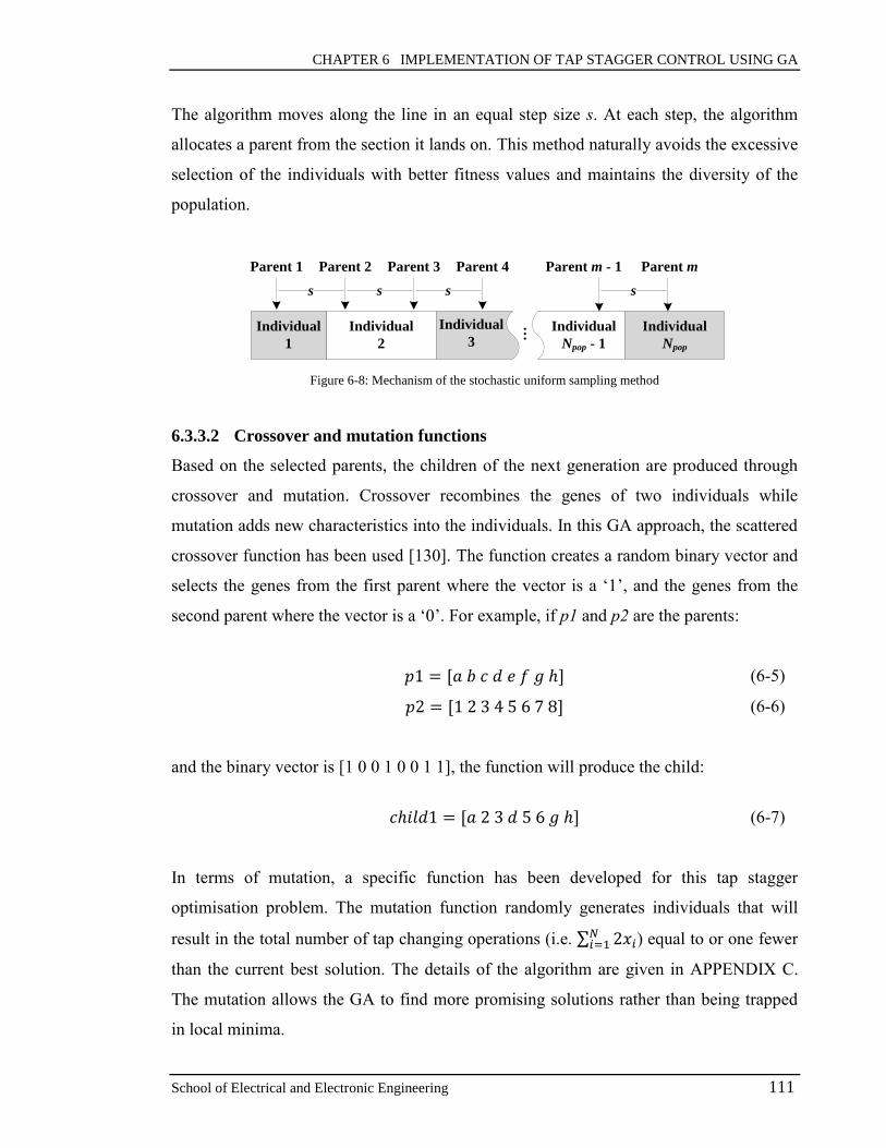
CHAPTER 6 IMPLEMENTATION OF TAP STAGGER CONTROL USING GA
School of Electrical and Electronic Engineering 111
The algorithm moves along the line in an equal step size s. At each step, the algorithm
allocates a parent from the section it lands on. This method naturally avoids the excessive
selection of the individuals with better fitness values and maintains the diversity of the
population.
…
Individual
1
Individual
2
Individual
3Individual
Npop - 1
Individual
Npop
Parent 1 Parent 2 Parent 3 Parent 4 Parent m - 1 Parent m
s s s s
Figure 6-8: Mechanism of the stochastic uniform sampling method
6.3.3.2 Crossover and mutation functions
Based on the selected parents, the children of the next generation are produced through
crossover and mutation. Crossover recombines the genes of two individuals while
mutation adds new characteristics into the individuals. In this GA approach, the scattered
crossover function has been used [130]. The function creates a random binary vector and
selects the genes from the first parent where the vector is a ‘1’, and the genes from the
second parent where the vector is a ‘0’. For example, if p1 and p2 are the parents:
𝑝1 = [𝑎 𝑏 𝑐 𝑑 𝑒 𝑓 𝑔 ℎ] (6-5)
𝑝2 = [1 2 3 4 5 6 7 8] (6-6)
and the binary vector is [1 0 0 1 0 0 1 1], the function will produce the child:
𝑐ℎ𝑖𝑙𝑑1 = [𝑎 2 3 𝑑 5 6 𝑔 ℎ] (6-7)
In terms of mutation, a specific function has been developed for this tap stagger
optimisation problem. The mutation function randomly generates individuals that will
result in the total number of tap changing operations (i.e. ∑ 2𝑥𝑖𝑁𝑖=1 ) equal to or one fewer
than the current best solution. The details of the algorithm are given in APPENDIX C.
The mutation allows the GA to find more promising solutions rather than being trapped
in local minima.

CHAPTER 6 IMPLEMENTATION OF TAP STAGGER CONTROL USING GA
School of Electrical and Electronic Engineering 112
6.3.4 Computational procedure
Figure 6-9 demonstrates the flowchart of the GA-based solution algorithm. As shown in
the figure, the algorithm includes a load flow module to calculate the network loss and
the actual VAr absorption due to the tap stagger. The initialisation requires the settings of
Qrequired, elimit and TSmax. When evaluating the fitness value, the algorithm will first set the
tap positions of OLTCs according to the chromosome x. Load flow will then be
performed to calculate the values of ∆Ploss and Qactual. Note that the OLTCs will remain at
the maximum or minimum positions if the constraint in Equation (4-20) is violated. The
GA process will stop if the maximum number of generations is reached or the best fitness
value in the population changes negligibly after several consecutive generations.
Start
Randomly generate an initial
population using Equation (6-1)
Calculate the fitness values
using Equation (6-2)
Stopping
criteria?
End
Output resultsSelection
Crossover Mutation
Next generation
(ngen = ngen + 1)
x: Check the constraint
of Equation (4-20)
Yes
No
Npop individuals
Npop
Ne elites
Npop – Ne
children mcr parents mmu parents
Initialisation
(Set Qrequired, elimit and TSmax)
m parents
∆Ploss, Qactual
Load flow
module
Figure 6-9: Flowchart of the GA-based solution procedure
CHAPTER 6 IMPLEMENTATION OF TAP STAGGER CONTROL USING GA
School of Electrical and Electronic Engineering 113
6.4 Testing of GA-based Control
The proposed GA-based control approach has been applied to the developed 102-bus
distribution network. The algorithm has been programmed using the MATLAB Global
Optimisation Toolbox [131] and the full codes are given in APPENDIX C. The OpenDSS
has been used to implement the load flow module shown in Figure 6-9.
6.4.1 Parameter assignment
As shown in Figure 6-1, the modelled distribution network has a total 11 pairs of primary
substation transformers available for the tap staggering operation, i.e. N = 11. The
network VAr absorption (Qactual), due to the tap stagger, is obtained by calculating the
reactive power flow variation at the GSP. Based on the Grid Code of National Grid [132],
the maximum permitted error (elimit) between Qrequired and Qactual has been set to 1%. The
distribution system loss (∆Ploss), due to the tap stagger is calculated by aggregating the
variations of the line and transformer losses. Considering the transformer health and
network loss, the maximum tap difference (TSmax) has been limited to 4 taps throughout
the simulations. Therefore, the search space for the GA is (1 + TSmax / 2) 11
= 311
=
177147. For Equation (6-2), w1, w2 and w3 have been normalised to balance the
influences of the power losses, OLTC switching and reactive power absorption on the
optimisation result. The details of the GA parameters are given in Table 6-2.
Table 6-2: Parameters of the GA optimisation algorithm
Parameter Value Parameter Value
Number of variables (N) 11 Population size (Npop) 100
elimit 1% Number of elites (Ne) 2
TSmax 4 Crossover fraction 0.5
w1 1 Maximum generations 100
w2 1/22 Stall generations 20
w3 1 Convergence tolerance 1×10⁻⁶

CHAPTER 6 IMPLEMENTATION OF TAP STAGGER CONTROL USING GA
School of Electrical and Electronic Engineering 114
The crossover fraction specifies the proportion of the next generation, other than elite
children, that are produced by the crossover. The algorithm will stop if the average
change in the fitness function value over Stall generations is less than the Convergence
tolerance. These GA parameters have been tuned through trial and error to obtain
accurate solutions with less time.
6.4.2 Optimisation results
6.4.2.1 Test with a single reactive power requirement
To demonstrate an example of the optimisation result, the GA approach has solved a
dispatch problem with the transmission system VAr requirement Qrequired = 0.5 MVAr.
Figure 6-10 demonstrated the data from the GA when it was running.
Figure 6-10: Information about individuals in each generation
As shown in the upper half of the figure, the best fitness value in the population has
converged quickly after just one generation. The lower half of Figure 6-10 indicates the
average distance between individuals, i.e. known as diversity. Diversity enables the GA
to search a larger region of space and it prevents premature convergence. The total
0 10 20 30 40 50 60 70 80 90 1000
50
100
Generation
Fitness v
alu
e
Best: 0.39094 Mean: 39.071
10 20 30 40 50 60 70 80 90 1002.5
3
3.5
4
Generation
Averg
ae D
ista
nce
Average Distance Between Individuals
Best f itness
Mean fitness

CHAPTER 6 IMPLEMENTATION OF TAP STAGGER CONTROL USING GA
School of Electrical and Electronic Engineering 115
computation time is 8.1s running on an i7-3.4GHz/8GB RAM computer and the final
solution is:
𝒙𝑜𝑝𝑡𝑖𝑚𝑎𝑙 = [0 0 0 0 0 0 0 2 0 0 2] (6-8)
which indicates that there would be 4 staggered taps on both the 8th
and 11th
pairs of
primary substation transformers (see Figure 6-1). The total number of switching
operations involved is 8; the introduced ∆Ploss is 0.027MW and the error between Qrequired
and Qactual is 0.95%. The solution xoptimal determines the arrangement of OLTC tap
positions while satisfying the VAr requirement.
6.4.2.2 Tests with different VAr requirements
Due to the random process of the GA, the algorithm may return a different solution each
time it runs. Therefore, statistical studies have been undertaken to analyse the accuracy
and precision of the algorithm. During the simulations, the value of Qrequired increased
from 0.1 MVAr to 2.5 MVAr with a step of 0.1 MVAr. The GA ran ten times for each
Qrequired and the statistic results are summarised in Table 6-3.
According to the table, for most Qrequired, the standard deviations of the optimisation
results over ten runs are zero. This implies that the GA can provide precise control of tap
stagger. In the situation where many feasible solutions exist in the search space (e.g.
Qrequired = 1.0 and 1.5 MVAr), it is more difficult to find the optimal solutions, resulting
in relatively large standard deviations. Note that the maximum limit of the staggered taps
TSmax can constrain the VAr absorption. For instance, at Qrequired = 2.5 MVAr, the
algorithm has returned large VAr absorption errors between Qrequired and Qactual, i.e. an
average of 3.095%. It has been observed that all the transformers have already used the
maximum staggered taps, i.e. 4 staggered taps. Consequently, no more reactive power can
be absorbed through the use of tap stagger. The network can only provide reactive power
absorption up to 2.4 MVAr with TSmax = 4.

CHAPTER 6 IMPLEMENTATION OF TAP STAGGER CONTROL USING GA
School of Electrical and Electronic Engineering 116
Table 6-3: Optimisation results with GA running ten times for each value of Qrequired (at elimit = 1% & TSmax = 4)
Qrequired
(MVAr)
Total tap operations Network loss due to
stagger (MW)
Error between Qrequired
and Qactual (%)
average standard
deviation average
standard
deviation average
standard
deviation
0.1 4 0 0.0094 0.0008 0.2134 0.3264
0.2 8 0 0.0146 0.0023 0.5346 0.3541
0.3 6 0 0.0113 0 0.6493 0
0.4 8 0 0.0198 0 0.8548 0
0.5 8 0 0.0273 0 0.9510 0
0.6 12 0 0.0273 0.0012 0.6732 0.1028
0.7 12 0 0.0264 0 0.2680 0
0.8 14 0 0.0383 0.0002 0.7264 0.1489
0.9 16 0 0.0355 0 0.1862 0.2076
1.0 16.2 0.6325 0.0497 0.0041 0.7980 0.0732
1.1 20 0 0.0443 0.0007 0.0853 0.0291
1.2 20 0 0.0532 0 0.7350 0
1.3 24 0 0.0553 0 0.3538 0
1.4 24 0 0.0628 0 0.0854 0
1.5 26.6 0.9661 0.0730 0.0027 0.6493 0.1551
1.6 28 0 0.0708 0 0.3857 0
1.7 30 0 0.0799 0.0013 0.7179 0.2786
1.8 32 0 0.0828 0 0.8252 0
1.9 34 0 0.0890 0.0014 0.5284 0.1782
2.0 36 0 0.1028 0 0.1008 0
2.1 38 0 0.1038 0 0.3736 0
2.2 40 0 0.1245 0 0.3481 0
2.3 42 0 0.1237 0 0.9078 0
2.4 44 0 0.1397 0 0.9425 0
2.5 44 0 0.1397 0 3.0952 0
Based on Table 6-3, Figure 6-11 illustrates the maximum, minimum and average values
of the ten optimisation results at each Qrequired. As shown in Figure 6-11a and Figure
6-11b, the total number of tap switching operations and network power losses increase
with the VAr requirement. As the VAr requirement increases, the tap stagger control
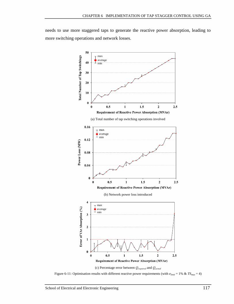
CHAPTER 6 IMPLEMENTATION OF TAP STAGGER CONTROL USING GA
School of Electrical and Electronic Engineering 117
needs to use more staggered taps to generate the reactive power absorption, leading to
more switching operations and network losses.
(a) Total number of tap switching operations involved
(b) Network power loss introduced
(c) Percentage error between Qrequired and Qactual
Figure 6-11: Optimisation results with different reactive power requirements (with elimit = 1% & TSmax = 4)
CHAPTER 6 IMPLEMENTATION OF TAP STAGGER CONTROL USING GA
School of Electrical and Electronic Engineering 118
In Figure 6-11c, the VAr absorption errors (between Qrequired and Qactual) change
randomly with respect to the VAr requirement, and most errors are below the predefined
1% tolerance. However, for Qrequired = 2.5 MVAr, the errors are higher than 1%. The large
errors have been introduced since all the transformers have reached the maximum limit of
staggered taps, i.e. 4 staggered taps. The network can only provide reactive power
absorption up to 2.4 MVAr under this constraint.
6.5 Effects of Different Load Models
As the use of tap stagger will draw more reactive power from the upstream networks, the
reactive currents between the 132kV and 33kV networks will increase. The HV voltages
of primary substations may drop, depending on the amount of VAr absorption produced
by tap stagger. Consequently, the LV voltages of primary substations may decrease as
well. The loads connected at the LV sides may change, depending on the relationship
between loads and voltages. In the simulations discussed above, the GA approach has
solved the VAr dispatch problems considering the network with constant power loads
connected at the primary substations. To further understand the impacts of load models
on the optimisation results, this section presents the studies with different load models.
The network load at each bus has been modelled as the following four static types [133]:
a) Constant power load.
b) Constant current magnitude load, with 𝑃 = 𝑃0 ∙𝑉
𝑉0 and 𝑄 = 𝑄0 ∙
𝑉
𝑉0, where P0 and Q0
are the active and reactive components of load when the bus voltage is V0.
c) Constant impedance load, with 𝑃 = 𝑃0 ∙ (𝑉
𝑉0)2 and 𝑄 = 𝑄0 ∙ (
𝑉
𝑉0)2.
d) 50% constant power load and 50% constant impedance load.
For each load model, the GA has solved the tap stagger optimisation problems with
different values of Qrequired (i.e. from 0.1 to 2.3 MVAr). The GA parameters have been set
according to Table 6-2. The algorithm has run once for each Qrequired and the
corresponding results are summarised in Table 6-4.
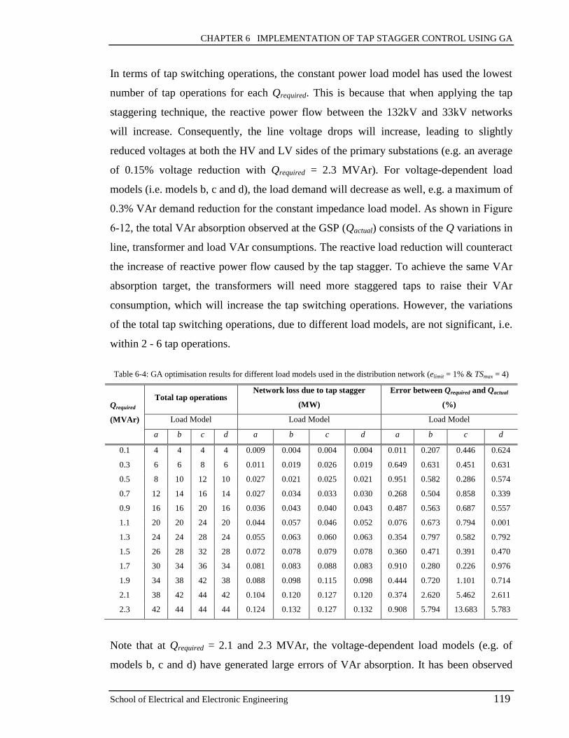
CHAPTER 6 IMPLEMENTATION OF TAP STAGGER CONTROL USING GA
School of Electrical and Electronic Engineering 119
In terms of tap switching operations, the constant power load model has used the lowest
number of tap operations for each Qrequired. This is because that when applying the tap
staggering technique, the reactive power flow between the 132kV and 33kV networks
will increase. Consequently, the line voltage drops will increase, leading to slightly
reduced voltages at both the HV and LV sides of the primary substations (e.g. an average
of 0.15% voltage reduction with Qrequired = 2.3 MVAr). For voltage-dependent load
models (i.e. models b, c and d), the load demand will decrease as well, e.g. a maximum of
0.3% VAr demand reduction for the constant impedance load model. As shown in Figure
6-12, the total VAr absorption observed at the GSP (Qactual) consists of the Q variations in
line, transformer and load VAr consumptions. The reactive load reduction will counteract
the increase of reactive power flow caused by the tap stagger. To achieve the same VAr
absorption target, the transformers will need more staggered taps to raise their VAr
consumption, which will increase the tap switching operations. However, the variations
of the total tap switching operations, due to different load models, are not significant, i.e.
within 2 - 6 tap operations.
Table 6-4: GA optimisation results for different load models used in the distribution network (elimit = 1% & TSmax = 4)
Qrequired
(MVAr)
Total tap operations Network loss due to tap stagger
(MW)
Error between Qrequired and Qactual
(%)
Load Model Load Model Load Model
a b c d a b c d a b c d
0.1 4 4 4 4 0.009 0.004 0.004 0.004 0.011 0.207 0.446 0.624
0.3 6 6 8 6 0.011 0.019 0.026 0.019 0.649 0.631 0.451 0.631
0.5 8 10 12 10 0.027 0.021 0.025 0.021 0.951 0.582 0.286 0.574
0.7 12 14 16 14 0.027 0.034 0.033 0.030 0.268 0.504 0.858 0.339
0.9 16 16 20 16 0.036 0.043 0.040 0.043 0.487 0.563 0.687 0.557
1.1 20 20 24 20 0.044 0.057 0.046 0.052 0.076 0.673 0.794 0.001
1.3 24 24 28 24 0.055 0.063 0.060 0.063 0.354 0.797 0.582 0.792
1.5 26 28 32 28 0.072 0.078 0.079 0.078 0.360 0.471 0.391 0.470
1.7 30 34 36 34 0.081 0.083 0.088 0.083 0.910 0.280 0.226 0.976
1.9 34 38 42 38 0.088 0.098 0.115 0.098 0.444 0.720 1.101 0.714
2.1 38 42 44 42 0.104 0.120 0.127 0.120 0.374 2.620 5.462 2.611
2.3 42 44 44 44 0.124 0.132 0.127 0.132 0.908 5.794 13.683 5.783
Note that at Qrequired = 2.1 and 2.3 MVAr, the voltage-dependent load models (e.g. of
models b, c and d) have generated large errors of VAr absorption. It has been observed

CHAPTER 6 IMPLEMENTATION OF TAP STAGGER CONTROL USING GA
School of Electrical and Electronic Engineering 120
that all the transformers have reached the maximum permitted staggering limit (TSmax)
and no extra reactive power can be absorbed to meet the VAr requirement. The VAr
absorption error can be reduced by increasing TSmax if allowed.
In addition, Table 6-4 indicates that the voltage-dependent load models have generally
resulted in more network losses (caused by tap stagger) than the constant impedance load
model. As explained before, the network with voltage-dependent loads will usually use
more staggered taps between the transformers to achieve the VAr absorption target. This
will further increase the transformer losses as well as the line losses between the 132kV
and 33kV networks. Consequently, the total network losses will increase. However, for
all the load models, the network losses introduced by tap stagger are much smaller (i.e.
90% less) than the reactive power absorption created.
33kV primary
substations
132kV GSPQactual
∆Qtransformers
∆Qlines
Qactual = ∆Qlines + ∆Qtransformers + ∆Qloads
∆Qloads
Figure 6-12: Reactive power absorption observed at the GSP by using the tap staggering technique
6.6 Time-Series Studies with Daily Load Profile
Since the demand for electricity changes continually in real distribution systems, it is
necessary to investigate the tap stagger optimisation at different load levels. As network
loads increase or decrease, the AVC relay needs to adjust the OLTC tap position to
maintain the bus voltage constant. Depending on the changed tap positions, the
optimisation result may be different from the previous load level.

CHAPTER 6 IMPLEMENTATION OF TAP STAGGER CONTROL USING GA
School of Electrical and Electronic Engineering 121
To carry out time-series studies, the load profile shown in Figure 6-13 has been used. It is
a typical daily load profile provided by the UK Energy Research Centre [134]. As
illustrated in the figure, there are 48 load points and each point represents the average
load during a half-hour period in a day. The network load is high from 18:00 to 21:00 and
decreases during the night. In the following studies, the original load of the 102-bus
distribution system has been taken as the peak load. At each time point, the load of each
bus has been modified by multiplying the percentage as indicated in Figure 6-13. Both
the active and reactive loads share the same profile.
Figure 6-13: Daily load profile used in the simulations (with half-hourly resolution)
With the daily load profile, time-series studies of the tap stagger optimisation have been
carried out. At each time point of the load curve, the tap positions of the primary
substation transformers were first calculated by the automatic voltage control to maintain
the secondary voltages at 1.0 pu. The tap stagger optimisation was then performed based
on the calculated tap positions. The automatic voltage control was disabled during the
optimisation process. By setting Qrequired = 1.0 MVAr, elimit = 1% and TSmax = 4, Figure
6-14 shows the 24-hour simulation results with different load models (i.e. constant power,
constant current magnitude and constant impedance).
In Figure 6-14a, the total number of switching operations used for tap stagger has varied
with the load level as expected. During periods of high demand (e.g. from 18:00 to 22:00),
the number of tap operations has fallen, since the additional VAr absorption of the lines

CHAPTER 6 IMPLEMENTATION OF TAP STAGGER CONTROL USING GA
School of Electrical and Electronic Engineering 122
(between the 132kV and 33kV networks) due to the tap stagger, has increased (see Figure
6-12). To achieve the same VAr absorption target, the tap stagger control can use fewer
staggered taps to reduce the transformer VAr absorption. In terms of the different load
models, the variations over the 24-hour period are similar. However, the constant
impedance load model has resulted in the largest number of switching operations. This is
due to the reactive load demand reduction as explained in Section 6.5. In addition, the
result of the constant impedance load model has frequently changed during a day since
the load is sensitive to the voltage variation.
Figure 6-14b shows the network loss introduced by the tap staggering operation during
the 24-hour period. For all three load models, the network losses introduced have not
followed the load profile. During periods of high demand, although the transmission line
losses have increased, the transformer losses have decreased as fewer staggered taps have
been used. These two factors have counteracted each other, resulting in not significant
changes in the total network losses (i.e. within 0.01 MW). In terms of the VAr absorption
error between Qrequired and Qactual, Figure 6-14c demonstrates that the error has changed
randomly between 0% and 1% over the 24-hour period. Figure 6-15 summarises the
average, maximum and minimum errors among the results. According to the figures, the
VAr absorption errors have been maintained below or close to the predefined 1%
tolerance, which satisfies the VAr requirement. From the results, the GA can provide
robust control of the tap stagger at different load levels.

CHAPTER 6 IMPLEMENTATION OF TAP STAGGER CONTROL USING GA
School of Electrical and Electronic Engineering 123
(a) Total number of tap switching operations involved
(b) Network power loss introduced
(c) Percentage error between Qrequired and Qactual
Figure 6-14: Optimisation results for the 102-bus network with 24-hour study (at Qrequired = 1.0 MVAr & elimit = 1%)
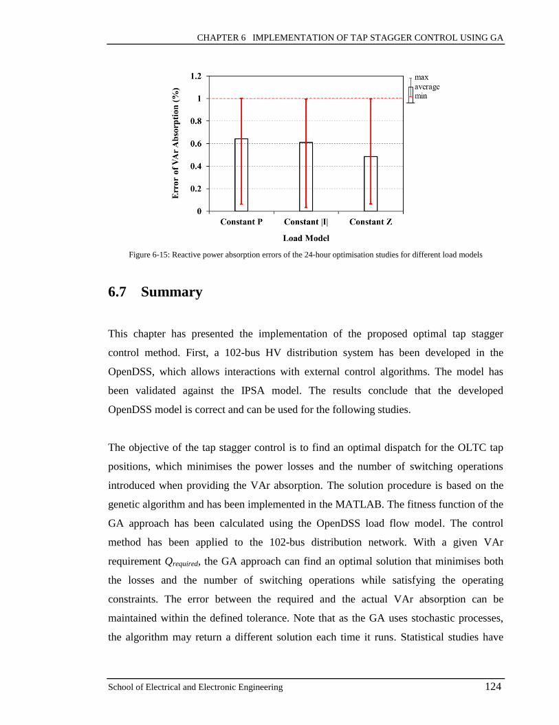
CHAPTER 6 IMPLEMENTATION OF TAP STAGGER CONTROL USING GA
School of Electrical and Electronic Engineering 124
Figure 6-15: Reactive power absorption errors of the 24-hour optimisation studies for different load models
6.7 Summary
This chapter has presented the implementation of the proposed optimal tap stagger
control method. First, a 102-bus HV distribution system has been developed in the
OpenDSS, which allows interactions with external control algorithms. The model has
been validated against the IPSA model. The results conclude that the developed
OpenDSS model is correct and can be used for the following studies.
The objective of the tap stagger control is to find an optimal dispatch for the OLTC tap
positions, which minimises the power losses and the number of switching operations
introduced when providing the VAr absorption. The solution procedure is based on the
genetic algorithm and has been implemented in the MATLAB. The fitness function of the
GA approach has been calculated using the OpenDSS load flow model. The control
method has been applied to the 102-bus distribution network. With a given VAr
requirement Qrequired, the GA approach can find an optimal solution that minimises both
the losses and the number of switching operations while satisfying the operating
constraints. The error between the required and the actual VAr absorption can be
maintained within the defined tolerance. Note that as the GA uses stochastic processes,
the algorithm may return a different solution each time it runs. Statistical studies have
CHAPTER 6 IMPLEMENTATION OF TAP STAGGER CONTROL USING GA
School of Electrical and Electronic Engineering 125
been carried out to analyse the accuracy and precision of the GA method. The results
confirm that the developed GA algorithm is capable of providing robust control for
different VAr absorption requirements.
In addition, the GA-based control approach has been investigated using different load
models. The results indicate that the algorithm will return solutions with more tap
switching operations if the network load is more sensitive to the voltage changes (e.g.
constant impedance load). This is because that when applying the tap staggering
technique, the line voltage drops between the 132kV and 33kV networks will increase.
The voltages at both the HV and LV sides of the primary substations will decrease as
well, resulting in lower load demands. The reduction in reactive load demands will
counteract the increase in reactive power flow caused by the tap stagger. To meet the
same VAr requirement, the control algorithm has to use more staggered taps to increase
the transformer VAr absorption. However, the results indicate that the variations of tap
switching operations, due to different load models, are not significant, i.e. within 2 - 6 tap
operations. The results also show that for voltage-dependant load models, the network
losses introduced are generally higher than the constant impendence load model when
applying the tap staggering technique. However, for all the load models, the network
losses introduced by tap stagger are much smaller (i.e. 90% - 95% less) than the reactive
power absorption created.
To investigate the GA performance under different load levels, case studies have been
carried out considering the network with a daily load profile. At each time point, the
OLTC tap positions have first been determined by the AVC relays and then adjusted by
the optimisation algorithm to achieve the VAr absorption requirement. The results show
that the GA approach can still maintain the VAr absorption error below the limit as the
load changes. During periods of high demand, the network can provide the VAr
absorption using fewer tap operations since the reactive power consumption of lines, due
to tap stagger, increases.
CHAPTER 7 COMPARISON OF GA WITH OTHER SOLUTION METHODS
School of Electrical and Electronic Engineering 126
CHAPTER 7
7 COMPARISON OF GA WITH OTHER SOLUTION
METHODS
7.1 Introduction
This chapter presents the comparison study between the tap stagger optimisation using
the GA approach and other solution methods. In the study, two alternative control
schemes have been developed based on the rule-based approach and the branch-and-
bound algorithm, respectively. Both methods utilise the information about the distribution
network VAr absorption capability. Sensitivity analysis is carried out to compare all three
control approaches using the 102-bus distribution network model presented in Chapter 6.
In addition, a new distribution network with 222 buses is modelled to represent a larger
network with higher demand. The control methods are investigated in the new model as
well. The details of the control principles and the optimisation results are discussed as
follows.
7.2 Alternative Control Methods for Tap Stagger
For the optimisation of tap stagger, a rule-based control scheme and a branch-and-bound
solution method have been developed so that they can be compared with the GA
approach. Both the control methods determine the OLTC tap positions with the
knowledge of network VAr absorption capability. As the implementation of the rule-
based control is straightforward, the result obtained can establish a baseline for the
comparison study. The branch-and-bound algorithm is a well-known method to solve
integer programming problems [135] and it is available in the MATLAB Optimisation
Toolbox. In addition, the algorithm is a deterministic method, which is different from the
random nature of the GA approach. The working principles of the rule-based and the
branch-and-bound control methods are described as follows.
CHAPTER 7 COMPARISON OF GA WITH OTHER SOLUTION METHODS
School of Electrical and Electronic Engineering 127
7.2.1 Rule-based control scheme
7.2.1.1 Matrix of reactive power absorption capability
When selecting the transformers to provide the VAr absorption service, the rule-based
control scheme always starts from the transformers that can absorb the largest reactive
power before those with the same staggered taps. This rule can help reduce the total
number of tap switching operations used. In order to know which transformers to select
first, the rule-based method utilises the information on the VAr absorption capability of
each primary substation transformer. The information can be described as a sensitivity
matrix:
𝑪 = [
𝐶1,1 ⋯ 𝐶1,𝑀
⋮ ⋱ ⋮𝐶𝑁,1 ⋯ 𝐶𝑁,𝑀
]
𝑁×𝑀
(7-1)
where N denotes the total pairs of parallel transformers, and 𝑀 = ⌊𝑇𝑆𝑚𝑎𝑥
2⌋, which is an
integer representing the maximum permitted taps to be staggered from the initial position.
The matrix element Ci,j indicates the VAr absorption that could be individually provided
by the ith
pair of parallel transformers with 2j staggered taps (i.e. j taps up for one and j
taps down for the other). The value of Ci,j can be obtained by pre-calculating the reactive
load flow change at the GSP with only the ith
pair tap staggering.
7.2.1.2 Control sequence
For a radial distribution network, the power flows of primary substations are usually
independent of each other. Therefore, when the network is required to provide reactive
power service, the rule-based control scheme can estimate the total VAr absorption
(Qactual) by summing up the MVArs from each primary substation. Figure 7-1
demonstrates the flowchart and the control steps are described as:
Step 1: Initialise all variables and define Qrequired, elimit, TSmax and the capability matrix
C. Set Qactual = 0, Cavailable = C.
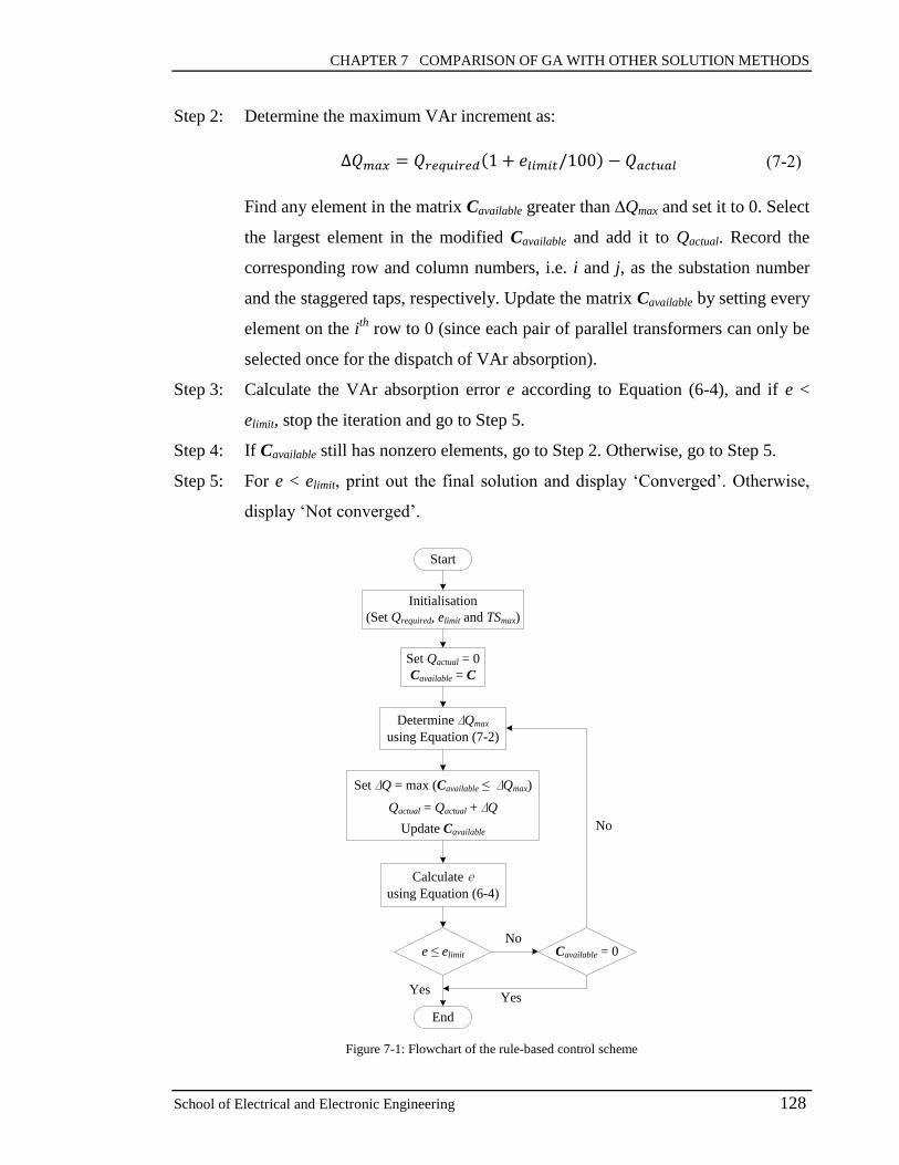
CHAPTER 7 COMPARISON OF GA WITH OTHER SOLUTION METHODS
School of Electrical and Electronic Engineering 128
Step 2: Determine the maximum VAr increment as:
∆𝑄𝑚𝑎𝑥 = 𝑄𝑟𝑒𝑞𝑢𝑖𝑟𝑒𝑑(1 + 𝑒𝑙𝑖𝑚𝑖𝑡/100) − 𝑄𝑎𝑐𝑡𝑢𝑎𝑙 (7-2)
Find any element in the matrix Cavailable greater than ∆Qmax and set it to 0. Select
the largest element in the modified Cavailable and add it to Qactual. Record the
corresponding row and column numbers, i.e. i and j, as the substation number
and the staggered taps, respectively. Update the matrix Cavailable by setting every
element on the ith
row to 0 (since each pair of parallel transformers can only be
selected once for the dispatch of VAr absorption).
Step 3: Calculate the VAr absorption error e according to Equation (6-4), and if e <
elimit, stop the iteration and go to Step 5.
Step 4: If Cavailable still has nonzero elements, go to Step 2. Otherwise, go to Step 5.
Step 5: For e < elimit, print out the final solution and display ‘Converged’. Otherwise,
display ‘Not converged’.
Start
Set Qactual = 0
Cavailable = C
Determine ∆Qmax
using Equation (7-2)
Initialisation
(Set Qrequired, elimit and TSmax)
Set ∆Q = max (Cavailable ≤ ∆Qmax)
Qactual = Qactual + ∆Q
Update Cavailable
Calculate e
using Equation (6-4)
e ≤ elimit Cavailable = 0
End
Yes
No
Yes
No
Figure 7-1: Flowchart of the rule-based control scheme

CHAPTER 7 COMPARISON OF GA WITH OTHER SOLUTION METHODS
School of Electrical and Electronic Engineering 129
Note that in Step 2, the algorithm chooses the largest VAr absorption available in order to
speed up the accumulation process and reduce the number of tap switching operations.
Although the rule-based control has not included the minimisation of network power loss,
the method provides a basic way to dispatch the VAr absorption with tap stagger.
7.2.2 Branch-and-bound solution method
7.2.2.1 Linearisation of the tap stagger optimisation problem
Based on the principles of the rule-based control, the branch-and-bound algorithm has
been adopted to minimise the network loss as well as the number of switching operations.
The algorithm searches for an optimal solution by solving a series of linear programming
(LP) relaxation problems [135]. To apply the algorithm, the tap stagger optimisation
problem has been linearised. First, the network power loss (due to tap stagger) can be
described by a sensitivity matrix:
𝑷 = [
𝑃1,1 ⋯ 𝑃1,𝑀
⋮ ⋱ ⋮𝑃𝑁,1 ⋯ 𝑃𝑁,𝑀
]
𝑁×𝑀
(7-3)
The matrix element Pi,j indicates the network loss caused by the ith
pair of parallel
transformers with 2j staggered taps (i.e. j taps up for one and j taps down for the other).
The value of Pi,j can be obtained by pre-calculating the network loss change with only the
ith
pair tap staggering.
For a radial distribution network, the objective in Equation (4-18) can be modified as:
min ∑∑(𝑃𝑖,𝑗 + 2𝑗)𝑥𝑖,𝑗
𝑀
𝑗=1
𝑁
𝑖=1
(7-4)
where the control variable xi,j is a binary integer 0 or 1. If xi,j = 1, the ith
pair of parallel
transformers will be tapped apart with 2j steps (i.e. j taps up for one and j taps down for

CHAPTER 7 COMPARISON OF GA WITH OTHER SOLUTION METHODS
School of Electrical and Electronic Engineering 130
the other). The coefficient Pi,j indicates the corresponding network loss introduced. Since
each pair of parallel transformers can only respond to a single command from the control
centre, the objective function is subject to:
∑𝑥𝑖,𝑗
𝑀
𝑗=1
≤ 1 for 𝑖 = 1,… ,𝑁 (7-5)
in addition to
|𝑄𝑟𝑒𝑞𝑢𝑖𝑟𝑒𝑑 − ∑ ∑ 𝐶𝑖,𝑗𝑥𝑖,𝑗
𝑀𝑗=1
𝑁𝑖=1 |
𝑄𝑟𝑒𝑞𝑢𝑖𝑟𝑒𝑑× 100% ≤ 𝑒𝑙𝑖𝑚𝑖𝑡 (7-6)
𝑇𝐴𝑃𝑖,𝑚𝑖𝑛 ≤ 𝑇𝐴𝑃𝑖 ± ∑𝑗𝑥𝑖,𝑗
𝑀
𝑗=1
≤ 𝑇𝐴𝑃𝑖,𝑚𝑎𝑥 (7-7)
With Equations (7-4)-(7-7), the non-linear tap stagger optimisation problem can be
transformed into a binary integer linear programming problem as:
min 𝐽 = min𝒙
𝒇𝑇𝒙 (7-8)
𝑨 ∙ 𝒙 ≤ 𝒃 (7-9)
where x is the solution vector with binary integers and the length is M×N. The
coefficients of the objective and constraint functions are:
𝒇 =
[
𝑃1,1 + 1
𝑃1,2 + 2
⋮𝑃1,𝑀 + 𝑀
𝑃2,1 + 1
⋮𝑃2,𝑀 + 𝑀
⋮𝑃𝑁,𝑀 + 𝑀]
(𝑀∙𝑁)×1
𝑨 = [𝑨1
𝑨2
𝑨3
] , 𝒃 = [
𝒃1
𝒃2
𝒃3
] (7-10)
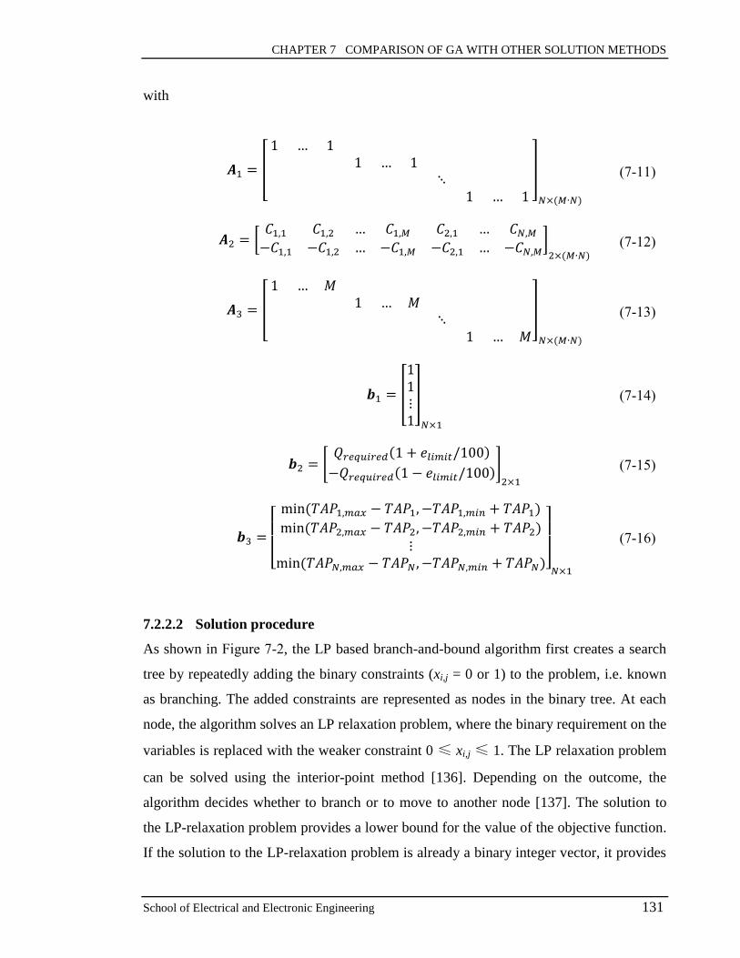
CHAPTER 7 COMPARISON OF GA WITH OTHER SOLUTION METHODS
School of Electrical and Electronic Engineering 131
with
𝑨1 = [
1 … 11 … 1
⋱1 … 1
]
𝑁×(𝑀∙𝑁)
(7-11)
𝑨2 = [𝐶1,1 𝐶1,2 … 𝐶1,𝑀 𝐶2,1 … 𝐶𝑁,𝑀
−𝐶1,1 −𝐶1,2 … −𝐶1,𝑀 −𝐶2,1 … −𝐶𝑁,𝑀]2×(𝑀∙𝑁)
(7-12)
𝑨3 = [
1 … 𝑀1 … 𝑀
⋱1 … 𝑀
]
𝑁×(𝑀∙𝑁)
(7-13)
𝒃1 = [
11⋮1
]
𝑁×1
(7-14)
𝒃2 = [𝑄𝑟𝑒𝑞𝑢𝑖𝑟𝑒𝑑(1 + 𝑒𝑙𝑖𝑚𝑖𝑡/100)
−𝑄𝑟𝑒𝑞𝑢𝑖𝑟𝑒𝑑(1 − 𝑒𝑙𝑖𝑚𝑖𝑡/100)]2×1
(7-15)
𝒃3 =
[ min (𝑇𝐴𝑃1,𝑚𝑎𝑥 − 𝑇𝐴𝑃1, −𝑇𝐴𝑃1,𝑚𝑖𝑛 + 𝑇𝐴𝑃1)
min (𝑇𝐴𝑃2,𝑚𝑎𝑥 − 𝑇𝐴𝑃2, −𝑇𝐴𝑃2,𝑚𝑖𝑛 + 𝑇𝐴𝑃2)⋮
min (𝑇𝐴𝑃𝑁,𝑚𝑎𝑥 − 𝑇𝐴𝑃𝑁 , −𝑇𝐴𝑃𝑁,𝑚𝑖𝑛 + 𝑇𝐴𝑃𝑁)]
𝑁×1
(7-16)
7.2.2.2 Solution procedure
As shown in Figure 7-2, the LP based branch-and-bound algorithm first creates a search
tree by repeatedly adding the binary constraints (xi,j = 0 or 1) to the problem, i.e. known
as branching. The added constraints are represented as nodes in the binary tree. At each
node, the algorithm solves an LP relaxation problem, where the binary requirement on the
variables is replaced with the weaker constraint 0 ≤ xi,j ≤ 1. The LP relaxation problem
can be solved using the interior-point method [136]. Depending on the outcome, the
algorithm decides whether to branch or to move to another node [137]. The solution to
the LP-relaxation problem provides a lower bound for the value of the objective function.
If the solution to the LP-relaxation problem is already a binary integer vector, it provides

CHAPTER 7 COMPARISON OF GA WITH OTHER SOLUTION METHODS
School of Electrical and Electronic Engineering 132
an upper bound for the objective value. As the search tree grows, the algorithm updates
the best solution as well as the lower and upper bounds on the objective function. The
bounds serve as the thresholds to cut off unnecessary branches. The maximum number of
nodes and the maximum time are used to terminate the process.
The branch-and-bound method could potentially try all the possible combinations of the
binary integers. The method searches the global optimum through a deterministic process
while the GA approach is based on a random process. The search space for the branch-
and-bound method is 2M×N
. For a large-scale distribution network, the search space will
increase significantly compared with the GA approach. However, as the branch-and-
bound method does not need to calculate load flows, the computation time may be faster
than the GA for small networks.
S00
S000 S001
S01
S010 S011
S10
S100 S101
S11
S110 S111
S0 S1
S
x1,1 = 0
x1,2 = 0
x1,1 = 1
x2,1 = 0
…… …………
Figure 7-2: Binary search tree [135]
7.3 Comparison Studies for 102-Bus Distribution Network
The two alternative control methods described above have been implemented in the
MATALB. The full codes are given in APPENDIX D. This section presents the tap
stagger optimisation studies of using the developed GA approach, the rule-based control
scheme and the branch-and-bound method. The results are compared with each other.
The 102-bus distribution system developed in the previous chapter has been used to test

CHAPTER 7 COMPARISON OF GA WITH OTHER SOLUTION METHODS
School of Electrical and Electronic Engineering 133
the tap stagger control. The studies started from the convergence analysis of each control
algorithm under different VAr requirements. To further compare the three control
methods, the studies also carried out the sensitivity analysis that investigated the impacts
of the input settings (i.e. elimit and TSmax) on the optimisation results. The details are
described as follows.
7.3.1 Case 1: Convergence analysis with different VAr requirements
The three tap stagger control methods have been applied to the 102-bus distribution
system shown in Figure 6-1. The VAr absorption target (Qrequired) has increased from 0.1
MVAr to 2.5 MVAr in a step of 0.1 MVAr and the algorithms have run once for each
target. The maximum permitted absorption error (elimit) and tap difference (TSmax) have
been set to 1% and 4, respectively. As described before, the rule-based control scheme
and the branch-and-bound method can only estimate the value of Qactual (or ∆Ploss) based
on the network VAr absorption matrix C (or the power loss matrix P). Therefore, after
obtaining the optimal tap positions, the two control methods have performed OpenDSS
load flow studies to calculate the actual values of Qactual and ∆Ploss. Table 7-1 summarises
the optimisation results of each control algorithm.
7.3.1.1 Reasons for non-convergence
In Table 7-1, the symbol ‘N/A’ indicates that the algorithm has not converged for the
corresponding VAr absorption requirement. Table 7-2 also lists the number of converged
solutions during the case study. According to the table, both the branch-and-bound and
the GA approaches provide more reliable tap stagger control than the rule-based method
does. In the solution process, the rule-based algorithm only attempts to use the
transformers with the largest VAr absorptions. This will increase the difficulty in
matching Qactual with Qrequired. For certain values of Qrequired, the final mismatch can still
exceed the elimit, leading to non-convergence of the iterative process.

CHAPTER 7 COMPARISON OF GA WITH OTHER SOLUTION METHODS
School of Electrical and Electronic Engineering 134
Table 7-1: Optimisation results for each value of Qrequired using different control algorithms (at elimit = 1% & TSmax = 4)
Qrequired
(MVAr)
Total tap operations Network loss due to stagger
(MW)a
Error between Qrequired and Qactual
(%)a
Rule
Based
Branch
and
Bound
GA
Rule
Based
Branch
and
Bound
GA
Rule
Based
Branch
and
Bound
GA
0.1 N/A 4 4 N/A 0.0107 0.0107 N/A 0.0107 0.6865
0.2 N/A 8 8 N/A 0.0120 0.0130 N/A 0.6140 0.9130
0.3 N/A 6 6 N/A 0.0114 0.0114 N/A 0.6493 0.6493
0.4 N/A 8 8 N/A 0.0198 0.0198 N/A 0.8548 0.8548
0.5 8 8 8 0.0330 0.0273 0.0273 0.3276 0.9510 0.9510
0.6 N/A 12 12 N/A 0.0229 0.0277 N/A 0.5214 0.7057
0.7 14 12 12 0.0359 0.0265 0.0265 0.6683 0.2680 0.2680
0.8 14 14 14 0.0432 0.0382 0.0382 0.5221 0.7692 0.7692
0.9 N/A 16 16 N/A 0.0356 0.0356 N/A 0.0573 0.4871
1 16 16 16 0.0516 0.0460 0.0516 0.7725 1.0552 0.7725
1.1 20 20 20 0.0563 0.0442 0.0442 0.4347 0.0761 0.0761
1.2 20 20 20 0.0636 0.0534 0.0534 0.1061 0.7350 0.7350
1.3 N/A 24 24 N/A 0.0554 0.0554 N/A 0.3538 0.3538
1.4 24 24 24 0.0830 0.0629 0.0629 0.7899 0.0854 0.0854
1.5 26 26 26 0.0727 0.0723 0.0723 0.1558 0.6970 0.6970
1.6 30 28 28 0.0804 0.0708 0.0708 0.2403 0.3857 0.3857
1.7 30 30 30 0.0844 0.0788 0.0788 0.1974 0.8488 0.8488
1.8 34 32 32 0.0920 0.0828 0.0828 0.1798 0.8252 0.8252
1.9 34 34 34 0.0960 0.0883 0.0918 0.2849 0.4439 0.8665
2 38 36 36 0.1048 0.1028 0.1028 0.2618 0.1008 0.1008
2.1 38 38 38 0.1139 0.1038 0.1038 0.2066 0.3736 0.3736
2.2 N/A 40 40 N/A 0.1245 0.1245 N/A 0.3481 0.3481
2.3 42 42 42 0.1339 0.1237 0.1237 0.7577 0.9078 0.9078
2.4 N/A N/A 44 N/A N/A 0.1397 N/A N/A 0.9425
2.5 N/A N/A 44 N/A N/A 0.1397 N/A N/A 3.0952
a. For the rule-based and the branch-and-bound methods, the values are calculated by running the
OpenDSS load flow model with the obtained optimal tap positions.
In terms of the branch-and-bound method, the approximation error caused by the
linearisation of the tap stagger control system may also result in non-convergence. For
instance, at Qrequired = 2.4 MVAr, the network can only achieve the VAr absorption target
by setting all the primary substations with 4 staggered taps. The error between Qrequired
and Qactual is 0.94% according to the GA result. However, the branch-and-bound method

CHAPTER 7 COMPARISON OF GA WITH OTHER SOLUTION METHODS
School of Electrical and Electronic Engineering 135
has calculated the error as 1.16% using Equation (7-6). As the error is higher than the
permitted limit 1%, the branch-and-bound cannot find any feasible solution in the search
space and therefore has returned ‘N/A’. Note that at Qrequired = 2.5 MVAr, both the rule-
based and branch-and-bound methods have not converged since all the primary substation
transformers have reached the stagger limit.
Table 7-2: Number of converged solutions for the VAr requirement from 0.1 to 2.5 MVAr
Rule-Based Branch-and-Bound GA
Number of converged solutions 15 23 25
7.3.1.2 Comparison of converged solutions
Table 7-3 shows the optimal solutions (i.e. x) obtained with different control algorithms
at Qrequired = 0.5, 1, 1.5 and 2 MVAr. According to the results, more pairs of transformers
and staggered taps need to be used as Qrequired increases. The corresponding number of tap
switching operations, power loss and absorption error are illustrated in Figure 7-3.
Table 7-3: Tap staggering arrangements of primary substations to provide reactive power absorption
NO. of
primary
sub
Rule-based method Branch-and-bound method GA approach
Qrequired (MVAr) Qrequired (MVAr) Qrequired (MVAr)
0.5 1.0 1.5 2.0 0.5 1.0 1.5 2.0 0.5 1.0 1.5 2.0
1 0 2 2 2 0 2 2 2 0 2 2 2
2 2 2 2 2 0 0 2 0 0 2 2 0
3 0 0 0 1 0 0 0 0 0 0 0 0
4 0 2 2 2 0 2 2 2 0 2 2 2
5 0 0 0 1 0 0 0 2 0 0 0 2
6 0 0 0 2 0 0 0 2 0 0 0 2
7 0 0 1 2 0 0 0 2 0 0 0 2
8 2 2 2 2 2 2 2 2 2 2 2 2
9 0 0 0 1 0 0 1 2 0 0 1 2
10 0 0 2 2 0 0 2 2 0 0 2 2
11 0 0 2 2 2 2 2 2 2 0 2 2
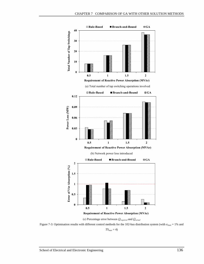
CHAPTER 7 COMPARISON OF GA WITH OTHER SOLUTION METHODS
School of Electrical and Electronic Engineering 136
(a) Total number of tap switching operations involved
(b) Network power loss introduced
(c) Percentage error between Qrequired and Qactual
Figure 7-3: Optimisation results with different control methods for the 102-bus distribution system (with elimit = 1% and
TSmax = 4)

CHAPTER 7 COMPARISON OF GA WITH OTHER SOLUTION METHODS
School of Electrical and Electronic Engineering 137
As shown in Figure 7-3a, both the branch-and-bound and the GA methods have returned
the same numbers of tap switching operations. For Qrequired = 2 MVAr, the rule-based
control scheme has led to two more switching operations than the other two methods.
In terms of the network loss, both the branch-and-bound and the GA approaches can
result in lower losses than the rule-based method (e.g. with average 5% less). The loss
reduction is not significant since most primary substation transformer models have
similar winding resistances. Therefore, the selection of different transformers for the tap
staggering will not have a great impact on the overall network loss. At Qrequired = 1 MVAr,
the branch-and-bound method has produced less network loss than the GA approach (see
Figure 7-3b). However, according to Figure 7-3c, the corresponding VAr absorption error
(between Qrequired and Qactual) of the branch-and-bound method is already higher than the
predefined limit 1%. This is due to the linearisation error as described before. In contrast,
the GA approach can still maintain the absorption error below 1%.
The computation time for the rule-based control scheme, the branch-and-bound method
and the GA approach is given in Table 7-4. Although the rule-based and the branch-and-
bound methods can provide much faster control than the GA approach, they deeply rely
on the linear characteristic of radial networks. However, the GA approach can be applied
to meshed distribution networks. In addition, the GA method can achieve more accurate
control as it calculates the VAr absorption through load flow studies rather than with the
linear approximation.
Table 7-4: Computation time for the 102-bus distribution system studies
Qrequired
(MVAr)
Computation Time (s)a
Rule-Based Branch-and-Bound GA
0.5 0.42 0.47 8.1
1.0 0.44 0.48 8.1
1.5 0.44 0.74 8.4
2.0 0.46 0.79 8.1
a. on MATLAB Version 7.11 and with i7-3.4 GHz / 8 GB RAM

CHAPTER 7 COMPARISON OF GA WITH OTHER SOLUTION METHODS
School of Electrical and Electronic Engineering 138
7.3.2 Case 2: Sensitivity analysis with different settings of reactive
power absorption accuracy
Case 1 has examined the convergence of each control algorithm with the maximum
permitted VAr absorption error (elimit) = 1%. To analyse the impact of elimit on the
optimisation results, this case study has tested the tap stagger control methods with
various settings of elimit. According to the Grid Code [132], if a generating unit is
instructed to provide a specific MVAr output, the generator must achieve that output
within a tolerance of +/- 5% of the rated output. Therefore, optimisation studies have
been carried out with elimit = 1%, 2%, 3%, 4% and 5%, respectively. For each setting of
elimit, the control algorithms have been tested with Qrequired = 0.5, 1, 1.5 and 2 MVAr.
TSmax has been set to 4 throughout the simulations. Table 7-5 summarises the simulation
results.
Based on the table, Figure 7-4 plots the number of tap switching operations, network loss
and VAr absorption error against the setting of elimit. For each elimit, the figures indicate
the average, maximum and minimum values of the results with the four different VAr
requirements (i.e. 0.5, 1, 1.5 and 2 MVAr).
According to Figure 7-4a, the total number of tap operations slightly decreases as elimit
increases. If the distribution network is allowed to provide the VAr absorption within a
larger tolerance, the control algorithms may be able to use smaller staggered taps to
satisfy the requirement. However, the reduction in tap switching operations is not
significant, e.g. only two tap operations for elimit = 5%. Note that the deviation between
the maximum and minimum numbers of tap operations at each elimit is large since the VAr
requirement Qrequired has changed from 0.5 to 2 MVAr. In other words, the number of tap
changing operations is more dependent on Qrequired than elimit.
Figure 7-4b shows the introduced network losses with different settings of elimit.
Compared with the rule-based control scheme, both the branch-and-bound and the GA
approaches can reduce the network loss caused by tap stagger. The loss reduction is more
effective as elimit increases, e.g. up to 18% reduction at elimit = 5%. Since a larger tolerance

CHAPTER 7 COMPARISON OF GA WITH OTHER SOLUTION METHODS
School of Electrical and Electronic Engineering 139
of VAr absorption can result in more feasible solutions, the GA algorithm (or the branch-
and-bound method) can find more promising solutions that introduce less network loss
while satisfying the constraints.
Table 7-5: Optimisation results with different settings of elimit (with TSmax = 4)
Total number of tap switching operations
elimit
Rule-based method Branch-and-bound method GA approach
Qrequired (MVAr) Qrequired (MVAr) Qrequired (MVAr)
0.5 1.0 1.5 2.0 0.5 1.0 1.5 2.0 0.5 1.0 1.5 2.0
1% 8 16 26 38 8 16 26 36 8 16 26 36
2% 8 16 26 38 8 16 26 36 8 16 26 36
3% 8 16 26 36 8 16 26 36 8 16 26 36
4% 8 16 24 36 8 16 24 36 8 16 24 36
5% 8 16 24 36 8 16 24 34 8 16 24 34
Network loss due to stagger (MW)a
elimit
Rule-based method Branch-and-bound method GA approach
Qrequired (MVAr) Qrequired (MVAr) Qrequired (MVAr)
0.5 1.0 1.5 2.0 0.5 1.0 1.5 2.0 0.5 1.0 1.5 2.0
1% 0.033 0.052 0.073 0.105 0.027 0.046 0.072 0.103 0.027 0.052 0.072 0.103
2% 0.027 0.052 0.073 0.105 0.019 0.046 0.065 0.100 0.019 0.046 0.065 0.100
3% 0.027 0.052 0.073 0.112 0.019 0.046 0.065 0.094 0.019 0.046 0.065 0.098
4% 0.027 0.052 0.070 0.112 0.019 0.044 0.070 0.092 0.019 0.044 0.070 0.098
5% 0.027 0.052 0.070 0.112 0.019 0.044 0.069 0.092 0.019 0.044 0.069 0.092
Error between Qrequired and Qactual (%)a
elimit
Rule-based method Branch-and-bound method GA approach
Qrequired (MVAr) Qrequired (MVAr) Qrequired (MVAr)
0.5 1.0 1.5 2.0 0.5 1.0 1.5 2.0 0.5 1.0 1.5 2.0
1% 0.328 0.773 0.156 0.262 0.951 1.055 0.697 0.101 0.951 0.773 0.697 0.101
2% 1.592 0.773 0.156 0.262 1.104 1.610 1.729 1.685 1.104 1.610 1.729 1.685
3% 1.592 0.773 0.156 2.451 1.104 1.610 2.270 3.085 1.104 1.610 2.270 2.272
4% 1.592 0.773 3.809 2.451 1.104 3.133 3.809 4.045 1.104 3.133 3.809 2.272
5% 4.117 0.773 3.809 2.451 1.104 4.630 4.825 4.734 1.104 4.630 4.825 4.734
a. For the rule-based and the branch-and-bound methods, the values are calculated by running the
OpenDSS load flow model with the obtained optimal tap positions.

CHAPTER 7 COMPARISON OF GA WITH OTHER SOLUTION METHODS
School of Electrical and Electronic Engineering 140
(a) Total number of tap switching operations involved
(b) Network power loss introduced
(c) Percentage error between Qrequired and Qactual
Figure 7-4: Optimisation results for the 102-bus distribution system using different settings of elimit (with Qrequired = 0.5
to 2 MVAr & TSmax = 4)

CHAPTER 7 COMPARISON OF GA WITH OTHER SOLUTION METHODS
School of Electrical and Electronic Engineering 141
In terms of the error between Qrequired and Qactual, Figure 7-4c indicates that the error
increases with elimit. The rule-based algorithm can return relatively small errors than the
branch-and-bound and the GA methods since these two methods need to consider the
minimisation of network losses. There is a trade-off among the minimisation of tap
operations, the loss reduction and the provision of the reactive power service. Note that
for elimit = 3% and 4%, the maximum VAr absorption errors from the branch-and-bound
method are slightly over the defined limits. This is because the method estimates the
value of Qactual using linear approximation rather than calculating it through load flow
studies.
7.3.3 Case 3: Sensitivity analysis with different settings of maximum
staggered taps
For the tap stagger control algorithms, there are three input settings, i.e. Qrequired, elimit and
TSmax. The previous Case 1 and Case 2 studies have investigated the impacts of Qrequired
and elimit on the optimisation results. Consequently, this case study aims to analyse the
performance of the tap stagger control with different settings of TSmax (i.e. the maximum
permitted staggered taps). As discussed in Section 4.3, the tap differences between
parallel transformers should be limited to prevent the transformers overheating and to
maintain secondary voltages constant. In addition, the OLTC of a primary substation
transformer usually has 15 to 18 available tap positions. Therefore, considering the
transformer rating as well as the headroom for tap staggering, this case study has
investigated the control algorithms with TSmax = 4, 6 and 8, respectively. For each setting
of TSmax, the algorithms have been tested with Qrequired = 0.5, 1, 1.5 and 2 MVAr. elimit has
been set to 1% throughout the simulations. Table 7-6 summarises the optimisation results.
According to Table 7-6, the total number of tap operations decreases significantly as
TSmax increases. For instance, comparing the results of TSmax = 4 and TSmax =8 at Qrequired
= 2.0 MVAr, the number of tap switching operations is reduced by 55% for all three
algorithms. Figure 7-5a also shows the average, maximum and minimum numbers of the
tap changing operations with the four different VAr requirements (i.e. 0.5, 1, 1.5 and 2
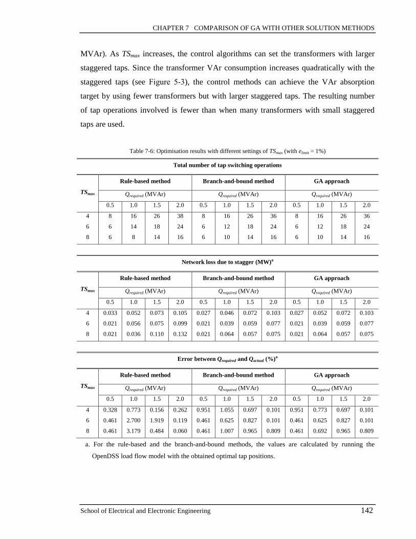
CHAPTER 7 COMPARISON OF GA WITH OTHER SOLUTION METHODS
School of Electrical and Electronic Engineering 142
MVAr). As TSmax increases, the control algorithms can set the transformers with larger
staggered taps. Since the transformer VAr consumption increases quadratically with the
staggered taps (see Figure 5-3), the control methods can achieve the VAr absorption
target by using fewer transformers but with larger staggered taps. The resulting number
of tap operations involved is fewer than when many transformers with small staggered
taps are used.
Table 7-6: Optimisation results with different settings of TSmax (with elimit = 1%)
Total number of tap switching operations
TSmax
Rule-based method Branch-and-bound method GA approach
Qrequired (MVAr) Qrequired (MVAr) Qrequired (MVAr)
0.5 1.0 1.5 2.0 0.5 1.0 1.5 2.0 0.5 1.0 1.5 2.0
4 8 16 26 38 8 16 26 36 8 16 26 36
6 6 14 18 24 6 12 18 24 6 12 18 24
8 6 8 14 16 6 10 14 16 6 10 14 16
Network loss due to stagger (MW)a
TSmax
Rule-based method Branch-and-bound method GA approach
Qrequired (MVAr) Qrequired (MVAr) Qrequired (MVAr)
0.5 1.0 1.5 2.0 0.5 1.0 1.5 2.0 0.5 1.0 1.5 2.0
4 0.033 0.052 0.073 0.105 0.027 0.046 0.072 0.103 0.027 0.052 0.072 0.103
6 0.021 0.056 0.075 0.099 0.021 0.039 0.059 0.077 0.021 0.039 0.059 0.077
8 0.021 0.036 0.110 0.132 0.021 0.064 0.057 0.075 0.021 0.064 0.057 0.075
Error between Qrequired and Qactual (%)a
TSmax
Rule-based method Branch-and-bound method GA approach
Qrequired (MVAr) Qrequired (MVAr) Qrequired (MVAr)
0.5 1.0 1.5 2.0 0.5 1.0 1.5 2.0 0.5 1.0 1.5 2.0
4 0.328 0.773 0.156 0.262 0.951 1.055 0.697 0.101 0.951 0.773 0.697 0.101
6 0.461 2.700 1.919 0.119 0.461 0.625 0.827 0.101 0.461 0.625 0.827 0.101
8 0.461 3.179 0.484 0.060 0.461 1.007 0.965 0.809 0.461 0.692 0.965 0.809
a. For the rule-based and the branch-and-bound methods, the values are calculated by running the
OpenDSS load flow model with the obtained optimal tap positions.

CHAPTER 7 COMPARISON OF GA WITH OTHER SOLUTION METHODS
School of Electrical and Electronic Engineering 143
(a) Total number of tap switching operations involved
(b) Network power loss introduced
(c) Percentage error between Qrequired and Qactual
Figure 7-5: Optimisation results for the 102-bus distribution system using different settings of TSmax (with Qrequired = 0.5
to 2 MVAr & elimit = 1%)

CHAPTER 7 COMPARISON OF GA WITH OTHER SOLUTION METHODS
School of Electrical and Electronic Engineering 144
Figure 7-5b shows the introduced network losses with different settings of TSmax.
Compared with the rule-based approach, both the branch-and-bound and the GA methods
can reduce the network loss due to tap stagger. The loss reduction is more significant as
TSmax increases, e.g. an average of 28% reduction at TSmax = 8. The setting of a larger
TSmax can allow the transformers to have a wider range of tap staggering. The GA
algorithm (or the branch-and-bound method) can find more combinations of the tap
staggering arrangements to reduce the power loss. Note that at each TSmax, the deviation
between the maximum and minimum network losses is quite large (i.e. greater than 300%)
since the VAr requirement Qrequired has changed from 0.5 to 2 MVAr. The large
deviations imply that the network loss introduced by tap stagger is predominated by
Qrequired.
In terms of the error between Qrequired and Qactual, Figure 7-5c indicates that the GA
approach is capable of maintaining the error below the limit of 1%. However, the rule-
based control scheme has returned large errors (i.e. up to 3%) for TSmax = 6 and 8. As the
rule-based algorithm only attempts to use the transformers with the largest VAr
absorptions in the solution process, the uncertainty of the mismatch between Qrequired and
Qactual is high. Consequently, the fulfilment of the VAr absorption requirement cannot be
guaranteed.
7.3.4 Summary of findings
For the 102-bus network model, three case studies have been carried out. Each case study
has investigated the impact of one of the control input settings on the optimisation results.
The input settings include the VAr absorption target Qrequired, the tolerance of VAr
absorption error elimit and the limit of maximum staggered taps TSmax.
Case 1 has analysed the convergence of each control algorithm with different values
of Qrequired. The result shows that the GA approach has converged for every Qrequired
and has maintained the VAr absorption error within the tolerance until the network
has reached its absorption limit. The rule-based algorithm can provide the fastest

CHAPTER 7 COMPARISON OF GA WITH OTHER SOLUTION METHODS
School of Electrical and Electronic Engineering 145
control while it does not consider the minimisation of network loss and it can lead to
non-convergence at certain values of Qrequired. The branch-and-bound method also
has a faster convergence speed than the GA. However, due to the errors caused by
the linearisation of the non-linear optimisation problem, the branch-and-bound
method may return solutions that violate the VAr absorption tolerance elimit. In
addition, both the rule-based and the branch-and-bound methods can only be applied
to radial distribution networks while the GA approach can also be used for meshed
networks.
Case 2 has carried out the sensitivity analysis that examined the three control
algorithms with different settings of elimit. Both the branch-and-bound and the GA
methods can result in lower network loss than the rule-based approach. The loss
reduction is more effective as elimit increases, e.g. up to 18% reduction at elimit = 5%.
The result also shows the VAr absorption error has increased with elimit.
Case 3 has investigated the impact of TSmax on the optimisation results. For all three
algorithms, the total number of tap operations has decreased as TSmax increases (e.g.
an average of 55% reduction from TSmax = 4 to TSmax =8). The results also indicate
that only the GA approach is capable of maintaining the VAr absorption error within
the tolerance under different settings of TSmax.
The total number of tap switching operations and the network loss due to tap stagger
are more dependent on Qrequired than elimit and TSmax. The VAr absorption error
changes randomly with Qrequired and TSmax, but it increases with elimit.
7.4 Comparison Studies for 222-Bus Distribution Network
The case studies in the previous section have investigated the tap stagger control methods
using the 102-bus distribution network model. The results indicate that the computation
time of the rule-based or the branch-and-bound methods is much faster than the GA
approach although the GA algorithm can provide more reliable and accurate solutions. To
further compare the three control methods, this section presents the optimisation studies
in a relatively large distribution system. A distribution network with 222 buses has been
modelled based on the distribution system described in Chapter 5. The 222-bus

CHAPTER 7 COMPARISON OF GA WITH OTHER SOLUTION METHODS
School of Electrical and Electronic Engineering 146
distribution network is part of the real UK HV distribution system studied in the ‘CLASS’
project [123]. It contains a 132kV GSP and the entire downstream 33kV networks
connected to the GSP. The network data and diagram are given in APPENDIX E.
Compared with the 102-bus distribution network model, the new network model has 28
pairs of primary substation transformers. With TSmax = 4, the search space for the GA
approach increases from 311
to 328
, and the search space for the branch-and-bound
method increases from 222
to 256
. Comparison studies have been carried out to analyse the
convergence and the computation time of each algorithm under this large-scale
distribution system. In addition, case studies have been undertaken to investigate the
control algorithms at different load levels. The details are discussed as follows.
7.4.1 Case 1: Convergence and computation time analyses with
different VAr requirements
The three tap stagger control algorithms have been applied to the 222-bus distribution
network and tested with the VAr absorption target from 0.5 MVAr to 7 MVAr in a step
of 0.5 MVAr. The algorithms have run once for each target. The values of elimit and TSmax
have been set to 1% and 4, respectively. The GA parameters have been defined according
to Table 6-2. As the search space has increased significantly, the maximum solution time
has been fixed to 3 minutes for both the GA and the branch-and-bound algorithms. Table
7-7 lists the optimisation results of each control algorithm.
According to the table, the rule-based and the branch-and-bound methods have not
converged at Qrequired = 7 MVAr. The GA approach also returned the solution with a large
VAr absorption error, i.e. 4.4%. It has been observed that all the transformers have
reached the maximum stagger limit, resulting in no more reactive power absorption. The
results imply that the network VAr absorption capability is below 7 MVAr with TSmax = 4.
7.4.1.1 Comparison of converged solutions
Figure 7-6 illustrates the numbers of tap switching operations, power losses and VAr
absorption errors introduced with different values of Qrequired. As shown in Figure 7-6a,
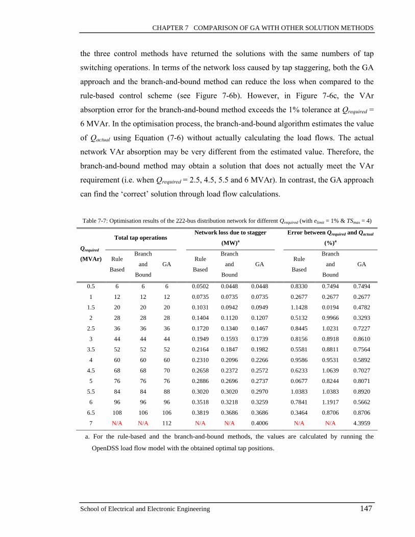
CHAPTER 7 COMPARISON OF GA WITH OTHER SOLUTION METHODS
School of Electrical and Electronic Engineering 147
the three control methods have returned the solutions with the same numbers of tap
switching operations. In terms of the network loss caused by tap staggering, both the GA
approach and the branch-and-bound method can reduce the loss when compared to the
rule-based control scheme (see Figure 7-6b). However, in Figure 7-6c, the VAr
absorption error for the branch-and-bound method exceeds the 1% tolerance at Qrequired =
6 MVAr. In the optimisation process, the branch-and-bound algorithm estimates the value
of Qactual using Equation (7-6) without actually calculating the load flows. The actual
network VAr absorption may be very different from the estimated value. Therefore, the
branch-and-bound method may obtain a solution that does not actually meet the VAr
requirement (i.e. when Qrequired = 2.5, 4.5, 5.5 and 6 MVAr). In contrast, the GA approach
can find the ‘correct’ solution through load flow calculations.
Table 7-7: Optimisation results of the 222-bus distribution network for different Qrequired (with elimit = 1% & TSmax = 4)
Qrequired
(MVAr)
Total tap operations Network loss due to stagger
(MW)a
Error between Qrequired and Qactual
(%)a
Rule
Based
Branch
and
Bound
GA
Rule
Based
Branch
and
Bound
GA
Rule
Based
Branch
and
Bound
GA
0.5 6 6 6 0.0502 0.0448 0.0448 0.8330 0.7494 0.7494
1 12 12 12 0.0735 0.0735 0.0735 0.2677 0.2677 0.2677
1.5 20 20 20 0.1031 0.0942 0.0949 1.1428 0.0194 0.4782
2 28 28 28 0.1404 0.1120 0.1207 0.5132 0.9966 0.3293
2.5 36 36 36 0.1720 0.1340 0.1467 0.8445 1.0231 0.7227
3 44 44 44 0.1949 0.1593 0.1739 0.8156 0.8918 0.8610
3.5 52 52 52 0.2164 0.1847 0.1982 0.5581 0.8811 0.7564
4 60 60 60 0.2310 0.2096 0.2266 0.9586 0.9531 0.5892
4.5 68 68 70 0.2658 0.2372 0.2572 0.6233 1.0639 0.7027
5 76 76 76 0.2886 0.2696 0.2737 0.0677 0.8244 0.8071
5.5 84 84 88 0.3020 0.3020 0.2970 1.0383 1.0383 0.8920
6 96 96 96 0.3518 0.3218 0.3259 0.7841 1.1917 0.5662
6.5 108 106 106 0.3819 0.3686 0.3686 0.3464 0.8706 0.8706
7 N/A N/A 112 N/A N/A 0.4006 N/A N/A 4.3959
a. For the rule-based and the branch-and-bound methods, the values are calculated by running the
OpenDSS load flow model with the obtained optimal tap positions.

CHAPTER 7 COMPARISON OF GA WITH OTHER SOLUTION METHODS
School of Electrical and Electronic Engineering 148
(a) Total number of tap switching operations involved
(b) Network power loss introduced
(c) Percentage error between Qrequired and Qactual
Figure 7-6: Optimisation results with different control methods for the 222-bus distribution system (with elimit = 1% and
TSmax = 4)

CHAPTER 7 COMPARISON OF GA WITH OTHER SOLUTION METHODS
School of Electrical and Electronic Engineering 149
7.4.1.2 Computation time
The computation time for each algorithm is given in Table 7-8. The rule-based algorithm
still provides the fastest control but it does not minimise the network loss. The average
time for the GA to solve a VAr dispatch problem is 22.3s, which is faster than the
average 78.9s of the branch-and-bound method. As the 222-bus network includes 28
primary substations, the search space is 328
for the GA, which is significantly less than
the 256
of the branch-and-bound algorithm. Consequently, the GA approach is more
efficient at finding feasible solutions and at identifying the optimal solution. Note that for
Qrequired = 3 MVAr (or 4 MVAr), there are many possible combinations of tap staggering
arrangements that can achieve the VAr absorption target. Therefore, the branch-and-
bound method has continued to search for the optimal solution and has only terminated
the iteration process after reaching the maximum solution time (i.e. 180s).
Table 7-8: Computation time for the 222-bus distribution system studies
Qrequired
(MVAr)
Computation Time (s)a
Rule-Based Branch-and-Bound GA
1 0.65 10.8 21.8
2 0.66 47.4 21.7
3 0.68 182.3 23.6
4 0.66 182.3 28
5 0.67 22.3 19.4
6 0.67 28.1 19.4
average 0.67 78.9 22.3
a. on MATLAB Version 7.11 and with i7-3.4 GHz / 8 GB RAM
7.4.2 Case 2: Comparison of time-series optimisation studies
Case 1 has investigated the three control methods in the 222-bus distribution system with
a fixed load level. This case study aims to analyse the performance of each control
algorithm with varying load demands. The daily load profile shown in Figure 6-13 has
been used. The original load of the 222-bus distribution system has been taken as the

CHAPTER 7 COMPARISON OF GA WITH OTHER SOLUTION METHODS
School of Electrical and Electronic Engineering 150
peak load. At each time point, the load of each bus has been modified by multiplying the
corresponding percentage indicated on the load profile. Load flow calculations with the
automatic voltage control (AVC) have then been performed to determine the initial tap
positions of the primary substation transformers. Based on the calculated tap positions,
the tap stagger optimal control has been carried out and the AVC has been disabled
during the optimisation process. For the rule-based and the branch-and-bound methods,
the matrices C and P have been recalculated at each time point. By setting Qrequired = 3
MVAr, elimit = 1% and TSmax = 4 throughout the 24-hour simulation, Figure 7-7 shows the
optimisation results with the three control methods.
In Figure 7-7a, the total number of tap switching operations varies with the load level.
During periods of high demand (e.g. 18:00 to 22:00), the number of tap operations
decreases since the additional VAr absorption of the lines (between the 132kV and 33kV
networks), due to the tap stagger, increases. To achieve the same VAr absorption target,
the control algorithms can use smaller staggered taps to reduce the transformer VAr
absorption. For the three control methods, the variations over the 24-hour period are
similar. However, the GA approach generally results in larger numbers of tap operations
than the other two methods. This is because the GA algorithm needs to consider the
fulfilment of the VAr absorption requirement as well as the minimisation of tap
operations. Figure 7-7c demonstrates the VAr absorption errors (between Qrequired and
Qactual) over the 24-hour period and Figure 7-8 summarises the average, maximum and
minimum errors among the 24-hour results. As shown in the figures, the GA method can
provide the VAr absorption within the 1% tolerance throughout the 24-hour period. In
contrast, the other two methods have several VAr absorption errors exceeding the limit at
certain time points.
Table 7-9 also lists the number of violations of the VAr requirement over the 24-hour
period with different settings of Qrequired. From the table, the GA algorithm has the least
number of violations among all the test results. The studies confirm that the GA approach
can provide accurate and robust control of the tap staggering operation under different
VAr absorption requirements and at various load levels.
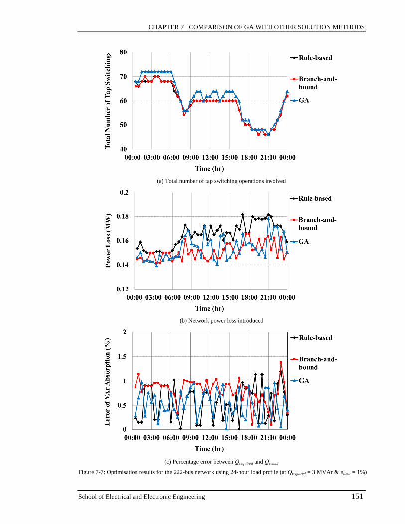
CHAPTER 7 COMPARISON OF GA WITH OTHER SOLUTION METHODS
School of Electrical and Electronic Engineering 151
(a) Total number of tap switching operations involved
(b) Network power loss introduced
(c) Percentage error between Qrequired and Qactual
Figure 7-7: Optimisation results for the 222-bus network using 24-hour load profile (at Qrequired = 3 MVAr & elimit = 1%)

CHAPTER 7 COMPARISON OF GA WITH OTHER SOLUTION METHODS
School of Electrical and Electronic Engineering 152
Figure 7-8: Reactive power absorption errors of the 24-hour optimisation studies for different solution methods
Table 7-9: 24-hour optimisation results for the 222-bus network with different settings of Qrequired
Qrequired
(MVAr)
Number of VAr requirement
violations (e > elimit) Computation time (s)
a
Rule
Based
Branch
and
Bound
GA Rule
Based
Branch
and
Bound
GA
1 6 3 0 13.1 4136.6 1092.9
2 1 13 1 13.1 7112.7 1154.3
3 4 6 0 13.2 5349.2 1105.2
4 5 19 1 13.2 3610.4 1096.8
5 2 3 0 13.3 1059.4 1021.8
6 2 0 0 13.7 238.0 976.6
a. The total computation time of the 24-hour optimisation study, based on MATLAB Version 7.11
and with i7-3.4 GHz / 8 GB RAM.
Figure 7-7b shows the network loss caused by the tap staggering operation during the 24-
hour period. Compared with the rule-based control scheme, the branch-and-bound
method has reduced the network loss by an average of 8% and the GA approach has an
average reduction of 6%. The loss reductions are not significant since most primary
substation transformers have similar winding resistances in the model. Consequently, the
selection of different transformers for the tap staggering will not have a great impact on

CHAPTER 7 COMPARISON OF GA WITH OTHER SOLUTION METHODS
School of Electrical and Electronic Engineering 153
the overall network loss. Although the branch-and-bound method can produce less loss
than the GA approach, the computation time is much longer than the GA approach for
this large network model (see Table 7-9).
7.4.3 Summary of findings
For the 222-bus distribution network model, two case studies have been carried out. The
first case study has analysed the computation time of each control algorithm in this larger
system. The result indicates that the computation time of the GA approach has become
faster than the branch-and-bound method since the search space has increased
significantly for the branch-and-bound algorithm. The second case study has investigated
the performance of each control method at different load levels, i.e. over a 24-hour period
of demand changing. Although the GA approach has resulted in slightly more tap
operations than the other two methods, the GA can provide the VAr absorption within the
defined tolerance throughout the 24-hour period. In contrast, both the rule-based and the
branch-and-bound methods have experienced several violations of the VAr absorption
requirement in the 24-hour period.
7.5 Summary
This chapter has presented the comparison studies of the tap stagger control using the
developed GA approach, the rule-based algorithm and the LP based branch-and-bound
method. The latter two methods have utilised the information of distribution network VAr
absorption capability (i.e. expressed as a sensitivity matrix). To apply the branch-and-
bound method, the tap stagger control problem has been linearised using the network
sensitivity matrices C and P. All three control approaches have been tested with the 102-
bus distribution network model and a relatively large distribution system with 222 buses.
Both network models are based on real UK HV distribution systems.
The key outcomes from the comparison studies can be summarised as:
CHAPTER 7 COMPARISON OF GA WITH OTHER SOLUTION METHODS
School of Electrical and Electronic Engineering 154
The rule-based control scheme provides the fastest control in both network models.
However, it does not consider the minimisation of network loss and may lead to non-
convergence.
The branch-and-bound method has a faster convergence speed than the GA approach
for the smaller network model (i.e. the 102-bus distribution network). However, due
to linearisation errors, the branch-and-bound method may return solutions that
violate the VAr absorption tolerance. In addition, for the larger system (i.e. the 222-
bus distribution network), the average computation time of the GA approach
becomes faster than the branch-and-bound method as the search space of the branch-
and-bound algorithm has increased significantly.
The GA approach provides the most accurate control, which maintains the VAr
absorption error within the tolerance under various input settings (i.e. Qrequired, elimit
and TSmax) and different load levels (i.e. with the daily load changing).
Both the rule-based and the branch-and-bound methods can only be applied to radial
distribution networks since they use the linear approximation to estimate the total
VAr absorption. However, the GA approach can also be used for meshed networks.
CHAPTER 8 IMPACTS OF TAP STAGGER ON TRANSMISSION SYSTEM
School of Electrical and Electronic Engineering 155
CHAPTER 8
8 IMPACTS OF TAP STAGGER ON TRANSMISSION
SYSTEM
8.1 Introduction
The studies in the previous chapters have focused on the feasibility and implementation
of the tap staggering technique. The reactive power absorption capability of distribution
networks through the use of tap stagger has been investigated. The control algorithms of
tap stagger have also been developed for distribution networks to provide the VAr
absorption service with the minimum number of tap switching operations and network
loss introduced. Therefore, based on the concept of utilising distribution networks to
support transmission VAr management, this chapter presents a comprehensive analysis of
both the economic and technical effects of the tap staggering technique on the
transmission system side. In the economic studies, the annual costs of applying the tap
staggering technique are investigated from the perspective of transmission system
operators. The IEEE Reliability Test System (RTS) load flow model is used to perform
the cost calculations under different scenarios. To demonstrate the economic benefit, the
results are compared with the use of the other passive compensator, i.e. shunt reactors. In
terms of the technical analysis, the transient responses of transmission voltages to the tap
staggering or reactor switching are investigated through dynamic studies. The details are
described as follows.
8.2 Transmission System Modelling and Tap Stagger
Implementation
8.2.1 IEEE reliability test system
The IEEE reliability test system (RTS) model has been used to investigate the impacts of
distribution network VAr absorption on the transmission system. The RTS network

CHAPTER 8 IMPACTS OF TAP STAGGER ON TRANSMISSION SYSTEM
School of Electrical and Electronic Engineering 156
comprises 24 buses connected by 33 lines and 5 transformers as shown in Figure 8-1.
There are a total 32 generating units, ranging from 12 to 400 MW. The transmission lines
are at two voltages, i.e. 138 kV and 230 kV. The system has voltage corrective devices at
bus 14 (synchronous condenser) and bus 6 (reactor). The complete network data are
available in [138] and the system has been modelled using the MATPOWER [139]. The
MATPOWER is a package of MATLAB programming files for solving power flow and
optimal power flow problems, especially for transmission systems.
BUS 1 BUS 2
BUS 3
BUS 4
BUS 5
BUS 6
BUS 7
BUS 8
BUS 9
BUS 10
BUS 11 BUS 12
BUS 13
BUS 14
BUS 15
BUS 16
BUS 17
BUS 18
BUS 19 BUS 20
BUS 21 BUS 22
BUS 23
BUS 24
cable
cable
230 kV
138 kV
Figure 8-1: Single-line diagram of the IEEE Reliability Test System

CHAPTER 8 IMPACTS OF TAP STAGGER ON TRANSMISSION SYSTEM
School of Electrical and Electronic Engineering 157
8.2.2 Identification of voltage problems
To identify the buses whose voltages are sensitive to load variations, an annual load flow
study has been performed. The annual load profile has been produced by combining the
weekly, daily and hourly load data from the original RTS system [138]. Figure 8-2 plots
the resulting load curve of 52×7×24=8736 hours.
Figure 8-2: Annual load profile for the RTS system (in percent of annual peak load)
In the RTS model, the default power rating for each load is the annual peak load and each
load is modelled as constant power load. The annual peak load for the overall RTS
system is 2850 MW. The load curve in Figure 8-2 indicates the hourly demand of the
system in the percentage of the annual peak load. The load profile has been applied to all
the network loads in order to simulate the power and voltage variations across a year. At
each time point, the load of each bus has been modified by multiplying the corresponding
percentage indicated on the load profile. Considering the balance between generation and
demand, the generating units have also changed their active power outputs according to
the load percentage. In addition, the generators have been set to maintain the voltages at
the connected buses by regulating their reactive power outputs within their capacities.
From the initial load flow study, only bus 6 and bus 10 have been observed with high
voltage violations (e.g. voltages larger than the normal operating limit 1.05 pu [140])

CHAPTER 8 IMPACTS OF TAP STAGGER ON TRANSMISSION SYSTEM
School of Electrical and Electronic Engineering 158
under light load conditions. This is due to the capacitive current produced by the cable
between bus 6 and bus 10. Although a 100 MVAr shunt reactor has already been placed
at bus 6 to absorb the VAr surplus, the voltage still exceeds the limit when demand is low.
Figure 8-3 illustrates the annual voltage profiles of buses 6 and 10. As shown in Figure
8-3a, the overvoltage issues at bus 6 have only occurred periodically for 358 hours over a
year (8736 hours). This implies that the permanent installation of an additional reactor at
bus 6 may not be cost-effective. However, Figure 8-3b shows that bus 10 has more
frequent voltage problems, i.e. 2000 hours during a year. The installation of a reactor may
need to be considered. The details of how to decide which technique is more cost-
effective to mitigate high voltage problems are given in Section 8.4.
(a) bus 6
(b) bus 10
Figure 8-3: Annual voltage profile of the RTS system
CHAPTER 8 IMPACTS OF TAP STAGGER ON TRANSMISSION SYSTEM
School of Electrical and Electronic Engineering 159
8.2.3 Implementation of tap stagger using GA
The tap staggering technique can be used to improve the voltage profiles of buses 6 and
10. As load buses (without generators connected) in the RTS system can be considered as
GSPs for distribution networks, the implementation of tap stagger can be achieved by
equivalently increasing the load consumption at buses 6 and 10. The increments in active
and reactive loads should be set to the same values as the power loss and reactive power
absorption introduced by the tap stagger, respectively. To determine the corresponding
power loss and VAr absorption, the 222-bus distribution network model in Chapter 7 has
been used.
Figure 8-4 illustrates the flowchart. The network model was integrated with the annual
load profile shown in Figure 8-2 and the tap stagger optimisation study was carried out
using the GA approach. The study started from the VAr absorption target (Qrequired) of 1
MVAr. With elimit = 1% and TSmax = 6 throughout the annual load flow study, the GA
calculated the actual network VAr absorption and the introduced network loss at each
time point, i,e. Qactual(t) and ∆Ploss(t). This procedure was repeated for Qrequired = 2, 3, …,
L MVAr. Considering the 222-bus network absorption limit, L was set to 10 MVAr for
this case. Based on the optimisation results, the following power variation matrices were
obtained:
∆𝑸(𝑡, 𝑛) = [
∆𝑄1,1 ⋯ ∆𝑄1,𝐿
⋮ ⋱ ⋮∆𝑄𝑇,1 ⋯ ∆𝑄𝑇,𝐿
]
𝑇×𝐿
(8-1)
∆𝑷(𝑡, 𝑛) = [
∆𝑃1,1 ⋯ ∆𝑃1,𝐿
⋮ ⋱ ⋮∆𝑃𝑇,1 ⋯ ∆𝑃𝑇,𝐿
]
𝑇×𝐿
(8-2)
where T denotes the total time points in a year, i.e. 8736. The matrix element ∆Qt,n
indicates the VAr absorption measured at the GSP with the VAr compensation level
(Qrequired) = n MVAr at the time point t. Similarly, the matrix ∆P(t, n) indicates the
network power losses due to the tap staggering at different time points.

CHAPTER 8 IMPACTS OF TAP STAGGER ON TRANSMISSION SYSTEM
School of Electrical and Electronic Engineering 160
In the RTS system, each load bus can be regarded as a GSP for distribution networks.
Therefore, if bus 6 or 10 needs to apply the tap staggering method, the matrices ∆Q(t, n)
and ∆P(t, n) will be used to determine the load increments, depending on the start time of
the staggering and the compensation level (Qrequired) used. The resulting impacts of the tap
stagger on the transmission system voltages and power generation are discussed in
Sections 8.3 and 8.4. As the study only involves static load flow calculations, the effects
of aggregating VAr absorption at the transmission level should be equivalent to the
effects of actually implementing tap stagger at distribution network transformers.
Start
Set Qrequired = n MVAr
Initialisation
Set n = 1
Run GA optimisation for the 222-bus network with
the annual load profile, obtain the introduced
network VAr absorption and power loss,
i.e. Qactual (t) and ∆Ploss (t)
Set ∆Q (t, n) = Qactual (t)
∆P (t, n) = ∆Ploss (t)
n = n + 1
n ≤ L
End
Yes
No
Figure 8-4: Flowchart to determine load increments when applying the tap staggering technique to the RTS system
CHAPTER 8 IMPACTS OF TAP STAGGER ON TRANSMISSION SYSTEM
School of Electrical and Electronic Engineering 161
8.2.4 Cost Analysis for VAr Compensation
The tap staggering technique is expected to provide a more cost-effective means of
absorbing VAr surplus than the traditional methods. To prove this potential benefit, the
cost for the transmission system operator (TSO) to use the tap staggering technique has
been analysed. As shunt reactors are widely installed to absorb the excess reactive power
in the grid, the associated costs have also been analysed and compared with the tap
staggering technique. The equations used to calculate the costs are described as follows.
8.2.4.1 Tap staggering technique
With the method described in Section 8.2.3, the associated cost for tap stagger can be
evaluated from the perspective of the TSO. In general, the TSO procures balancing
services to balance demand and supply and to control the system frequency and voltage
across the transmission system. As the use of tap stagger will increase the active power
demands, more power may need to be generated to maintain the system frequency within
the statutory limits. Consequently, the TSO may pay the generators for producing the
extra power [141]. Additionally, the TSO shall pay the reactive power service providers
for supporting the system voltages. Therefore, considering the VAr supports provided by
distribution networks as ancillary services, the annual cost for the TSO to apply the tap
staggering technique can be derived as:
𝐶𝑠𝑡𝑎𝑔𝑔𝑒𝑟 = 𝐶∆𝑔𝑒𝑛(ℎ) + 𝐶𝑉𝐴𝑟 ∑ ∆𝑄𝑡𝑚 ∙ ∆ℎ
ℎ
𝑚=1
(8-3)
where h denotes the total hours of using tap stagger in a year (i.e. the utilisation hour).
The first term C∆gen(h) represents the cost to compensate the generation changes and it
can be calculated using the generator cost data. The second term represents the payment
for VAr support providers, i.e. the distribution network operators. The payment is
calculated based on the unit price of reactive energy CVAr (in £/MVArh). ∆𝑄𝑡𝑚 denotes
the total VAr absorption (in MVAr) provided through the use of tap stagger at the time
CHAPTER 8 IMPACTS OF TAP STAGGER ON TRANSMISSION SYSTEM
School of Electrical and Electronic Engineering 162
point tm (m = 1, 2, …, h) and ∆h is the time interval, taken as 1 hour for the following
studies.
8.2.4.2 Installation of shunt reactor
To compare it with the tap stagger, the cost of employing shunt reactors has also been
analysed. For the TSO, a capital investment needs to be paid to purchase and install a
reactor. The annual equivalent investment cost I can be calculated as [76]:
𝐼 = 𝑆𝑟(1 + 𝑟)𝑦
(1 + 𝑟)𝑦 − 1 (8-4)
where S is the actual capital investment, which depends on the reactor rating (in MVAr),
r is the discount rate and y is the economic life of the reactor. As the use of shunt reactor
could reduce the reactive power flow during periods of low demand, the network power
loss would also decrease. The TSO may pay less for the generation used to balance the
system frequency. Therefore, without considering the maintenance cost of the reactor, the
annual cost for the TSO to use a reactor can be described as:
𝐶𝑟𝑒𝑎𝑐𝑡𝑜𝑟 = 𝐶∆𝑔𝑒𝑛′(ℎ) + 𝐼 (8-5)
where C∆gen’(h) denotes the cost for generation changes, which could be negative [141] as
the reactor could reduce the network power loss during periods of low demand.
8.3 Effectiveness on Voltage Regulation
In this section, the effectiveness of the tap staggering technique on mitigating high
voltages has been demonstrated. First, annual load flow studies have been performed
considering the RTS system with the tap staggering method applied to bus 6. At each
time point, the tap stagger would only be activated if the corresponding bus voltage
exceeded the normal operating limit 1.05 pu. The tap staggering method would increase
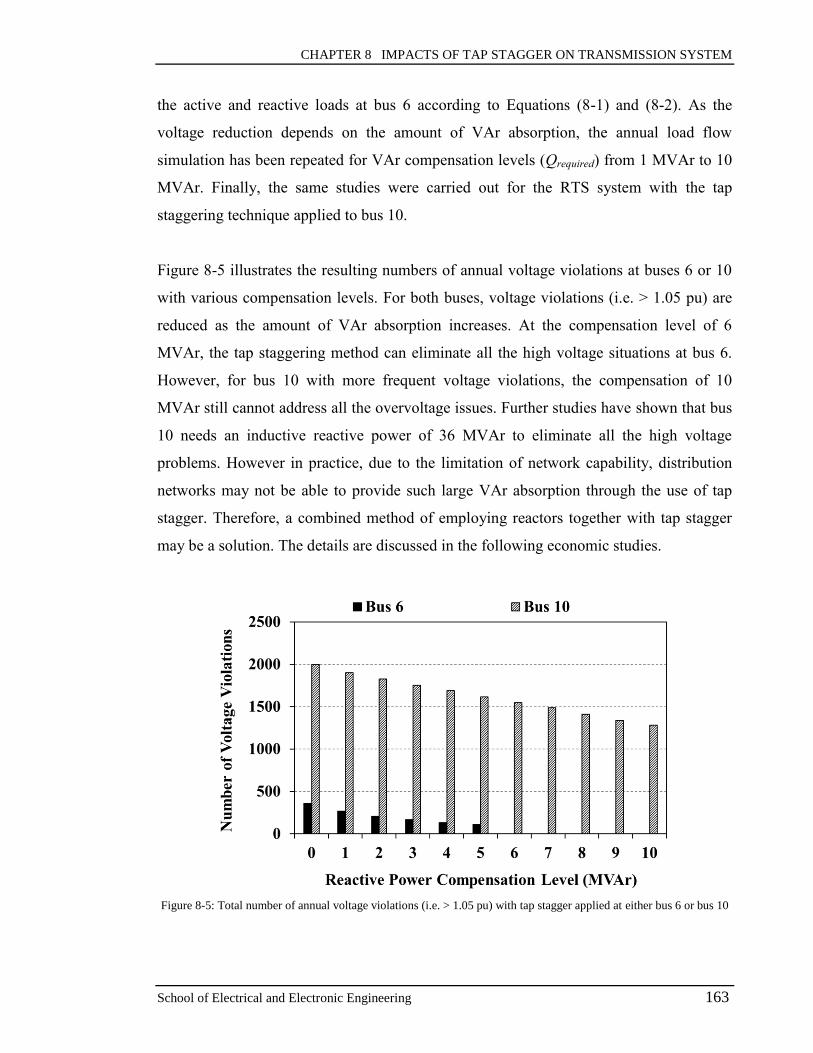
CHAPTER 8 IMPACTS OF TAP STAGGER ON TRANSMISSION SYSTEM
School of Electrical and Electronic Engineering 163
the active and reactive loads at bus 6 according to Equations (8-1) and (8-2). As the
voltage reduction depends on the amount of VAr absorption, the annual load flow
simulation has been repeated for VAr compensation levels (Qrequired) from 1 MVAr to 10
MVAr. Finally, the same studies were carried out for the RTS system with the tap
staggering technique applied to bus 10.
Figure 8-5 illustrates the resulting numbers of annual voltage violations at buses 6 or 10
with various compensation levels. For both buses, voltage violations (i.e. > 1.05 pu) are
reduced as the amount of VAr absorption increases. At the compensation level of 6
MVAr, the tap staggering method can eliminate all the high voltage situations at bus 6.
However, for bus 10 with more frequent voltage violations, the compensation of 10
MVAr still cannot address all the overvoltage issues. Further studies have shown that bus
10 needs an inductive reactive power of 36 MVAr to eliminate all the high voltage
problems. However in practice, due to the limitation of network capability, distribution
networks may not be able to provide such large VAr absorption through the use of tap
stagger. Therefore, a combined method of employing reactors together with tap stagger
may be a solution. The details are discussed in the following economic studies.
Figure 8-5: Total number of annual voltage violations (i.e. > 1.05 pu) with tap stagger applied at either bus 6 or bus 10

CHAPTER 8 IMPACTS OF TAP STAGGER ON TRANSMISSION SYSTEM
School of Electrical and Electronic Engineering 164
8.4 Economic Studies
This section presents the cost analysis of applying the tap staggering technique when high
voltage problems arise occasionally or frequently. The results have been compared to the
use of shunt reactors. The RTS system has been tested under three different scenarios to
demonstrate the economic benefit of applying tap stagger.
8.4.1 Case 1: Cost analysis for bus with occasional voltage issues
As shown in Figure 8-1, the RTS network already has a shunt reactor of 100 MVAr
connected at bus 6 to absorb the capacitive reactive power. From the voltage regulation
study result shown in Figure 8-5, bus 6 still requires an additional inductive reactive
power of 6 MVAr to eliminate all the high voltage problems. Therefore, in this case study,
two solution methods have been used to mitigate the high voltages, which are:
Solution 1: Installing an additional shunt reactor of 6 MVAr at bus 6,
Solution 2: Applying the tap staggering method described in Section 8.2.3 at bus 6 with
the compensation level (Qrequired) of 6 MVAr.
Annual load flow studies have been performed considering the system with the two
solution methods separately. Note that for both methods, the VAr compensation would
only be activated when bus 6 and/or bus 10 voltages exceeded the normal operating limit
1.05 pu during the simulations. The total utilisation hours for each method are 2000 hrs as
bus 10 has experienced the most voltage violations, i.e. for 2000 hrs.
According to Equations (8-3) and (8-5), the cost calculations of both solution methods
have considered the impacts of generation changes. Intuitively, the tap staggering method
should be less expensive than the use of reactors as no extra capital investment is required.
However, since the employment of tap stagger also increases the active power demands,
more energy needs to be produced to balance the power flow, resulting in more
generation costs. Figure 8-6 indicates the annual energy generation for the RTS system

CHAPTER 8 IMPACTS OF TAP STAGGER ON TRANSMISSION SYSTEM
School of Electrical and Electronic Engineering 165
with the two solution methods, respectively. As shown in the figure, the generation
changes with the utilisation hours of the methods. Solution 1 can reduce the energy
generation as the network power loss decreases when the reactor is connected. For
solution 2, the energy generation increases with the utilisation hours. However, as the tap
staggering method only slightly increases the demands, the increase in energy generation
is very small, e.g. 0.003% for 2000 hrs of utilisation.
Figure 8-6: Annual energy generation for the RTS system with either reactor or tap stagger
With Equations (8-3) and (8-5), the annual costs of solutions 1 and 2 have been evaluated.
First, the costs to compensate generation changes, i.e. C∆gen(h) and C∆gen’(h), have been
calculated based on the generator cost data from [138]. For solution 1, the capital
investment of a high-voltage reactor has been estimated as 37×103 £/MVAr [142]. By
applying an economic life of 38 years [76] and a discount rate of 8% to Equations (8-4),
the annual equivalent investment cost of a reactor has been estimated as 3182 £/MVAr
per year. In solution 2, the unit price of reactive energy has been assumed as 3.2
£/MVArh [143]. Considering the compensation level of 6 MVAr, Figure 8-7 plots the
annual costs of both methods against the utilisation hour h.
According to the figure, the cost of using a reactor starts from the annual equivalent
investment 6 × 3182 = 1.9×10⁴ £ and decreases with the number of utilisation hours since
the cost of energy generation has been reduced. In contrast, the cost of applying tap

CHAPTER 8 IMPACTS OF TAP STAGGER ON TRANSMISSION SYSTEM
School of Electrical and Electronic Engineering 166
stagger starts from 0 and increases with the number of utilisation hours. From the result,
the tap staggering technique is more economical than the use of a reactor up to a
maximum of 612 utilisation hrs. As bus 6 initially has 358 hrs of voltage violations, the
use of tap stagger can eliminate all the voltage issues but cost 40% less than the
installation of the reactor as shown in the figure.
Figure 8-7: Annual costs for solutions 1 and 2 in Case 1 (at compensation level of 6 MVAr)
8.4.2 Case 2: Cost analysis for bus with frequent voltage issues
From Case 1, the high voltage problems at bus 6 have been solved by applying an
additional reactor or the tap staggering method directly at bus 6. However, the adjacent
bus 10 still has a large number of voltage violations according to Figure 8-5. To reduce
the high voltages, another two methods have been adopted, which are:
Solution 3: Installing shunt reactors at buses 6 and 10,
Solution 4: Applying tap stagger at buses 6 and 10.
In solution 3, both buses 6 and 10 have a shunt reactor installed, with a rating of 6 MVAr.
For solution 4, the compensation levels (Qrequired) at both buses have been set to 6 MVAr.
For each method, the VAr compensation at each bus would only be activated if the

CHAPTER 8 IMPACTS OF TAP STAGGER ON TRANSMISSION SYSTEM
School of Electrical and Electronic Engineering 167
corresponding bus had high voltage violations. The annual costs for solutions 3 and 4
have been calculated using the same parameters as in Case 1. From the results shown in
Figure 8-8, the tap staggering method is less expensive than the installation of reactors for
utilisation hours up to 1069 hrs. However, as stated earlier, bus 10 initially has 2000 hrs
of voltage violations, which require 2000 hrs of using tap stagger to reduce the high
voltages. Therefore, it is more advisable to install shunt reactors than to apply tap stagger
in this case. Note that the placement of the 6 MVAr reactors still cannot completely
resolve the voltage issues at bus 10 (see Figure 8-5). The installation of larger rating
reactors may be a solution but with higher capital investments. To reduce the cost, a
combined method of using both reactor and tap stagger is investigated in the following
case study.
Figure 8-8: Annual costs for solutions 3 and 4 in Case 1 (at compensation level of 6 MVAr)
8.4.3 Case 3: Combined method of reactor and tap Stagger
The result of Case 2 indicates that the installation of reactors will be more cost-effective
than tap stagger if high voltage situations occur frequently. This case study aims to
analyse the cost of applying the combined method of using both reactor and tap stagger.
According to load flow studies, an inductive compensation of 4 MVAr at bus 6 together
with a compensation of 28 MVAr at bus 10 can eliminate all the voltage violations during

CHAPTER 8 IMPACTS OF TAP STAGGER ON TRANSMISSION SYSTEM
School of Electrical and Electronic Engineering 168
periods of low demand. Therefore, considering the limitation of VAr absorption provided
through the use of tap stagger, three solution methods have been investigated:
Solution 5: Installing a reactor of 4 MVAr at bus 6 & installing a reactor of 28 MVAr at
bus 10,
Solution 6: Applying tap stagger of 4 MVAr (i.e. Qrequired = 4 MVAr) at bus 6 & installing
a reactor of 28 MVAr at bus 10,
Solution 7: Applying tap stagger of 4 MVAr at bus 6 & installing a reactor of 24 MVAr
and applying tap stagger of 4 MVAr at bus 10.
In solution 7, the tap stagger at bus 6 and the reactor at bus 10 had been first used to
absorb reactive power surplus when the corresponding bus had voltage violations. If the
voltage at bus 10 was still higher than the limit, the tap staggering method for bus 10
would be activated to reduce the voltage further. Table 8-1 summarises the annual costs
for the three solution methods along with the utilisation hours of tap staggering.
Table 8-1: Annual costs for solutions 5, 6 and 7 in case 3
Solution method
Utilisation hour of
tap stagger (hrs)
Annual
cost
(£/year)
Cost
reduction Bus 6 Bus 10
Solution 5
(reactors only) 0 0 0.992 x10
5 0
Solution 6
(stagger at bus 6 & reactor at bus 10) 358 0 0.941 x10
5 5%
Solution 7
(stagger at bus 6 & reactor + stagger at bus 10) 358 187 0.848 x10
5 15%
From the table, the costs of combined methods (i.e. solutions 6 and 7) are less than the
cost of only using reactors (i.e. solution 5). Comparing solutions 5 and 6, it is more
economical to apply tap stagger than reactor at bus 6, where high voltage problems occur
occasionally. For bus 10, which experiences frequent overvoltages, an integrated method

CHAPTER 8 IMPACTS OF TAP STAGGER ON TRANSMISSION SYSTEM
School of Electrical and Electronic Engineering 169
of using tap stagger and a reactor with small rating can help reduce the VAr
compensation cost (e.g. by 15% in solution 7).
8.5 Dynamic Performance Studies
In addition to the economic studies, the dynamic impacts of the tap stagger switching on
the transmission system have been investigated. The RTS system in Figure 8-1 has been
modelled using the DIgSILENT to perform the transient analyses [144]. To simulate an
equivalent distribution network for tap staggering, five pairs of primary substation
transformers have been modelled and connected to bus 6 through a 132/33 kV
transformer (see Figure 8-9). The line and transformer parameters have been obtained
from the 222-bus distribution network model studied in Chapter 7, and 50% of the
original load at bus 6 has been distributed evenly through the five primary substations.
The resulting demand for each primary substation is around 13 MW, which is close to the
default load rating of the 222-bus network. According to the capability studies presented
in Chapter 5, five primary substations can provide a total 1 MVAr absorption with four
staggered taps (i.e. two taps up for one transformer and two taps down for the other).
RTS Network
BUS 6
reactor
Primary
Substation
Figure 8-9: Modified RTS system for dynamic studies
The successive switching of OLTCs in the distribution substations can affect the voltages
at the upstream transmission buses. The resulting voltage responses have been compared
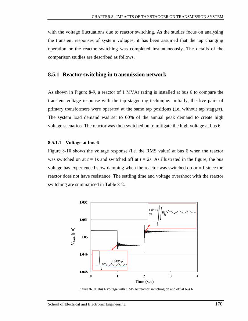
CHAPTER 8 IMPACTS OF TAP STAGGER ON TRANSMISSION SYSTEM
School of Electrical and Electronic Engineering 170
with the voltage fluctuations due to reactor switching. As the studies focus on analysing
the transient responses of system voltages, it has been assumed that the tap changing
operation or the reactor switching was completed instantaneously. The details of the
comparison studies are described as follows.
8.5.1 Reactor switching in transmission network
As shown in Figure 8-9, a reactor of 1 MVAr rating is installed at bus 6 to compare the
transient voltage response with the tap staggering technique. Initially, the five pairs of
primary transformers were operated at the same tap positions (i.e. without tap stagger).
The system load demand was set to 60% of the annual peak demand to create high
voltage scenarios. The reactor was then switched on to mitigate the high voltage at bus 6.
8.5.1.1 Voltage at bus 6
Figure 8-10 shows the voltage response (i.e. the RMS value) at bus 6 when the reactor
was switched on at t = 1s and switched off at t = 2s. As illustrated in the figure, the bus
voltage has experienced slow damping when the reactor was switched on or off since the
reactor does not have resistance. The settling time and voltage overshoot with the reactor
switching are summarised in Table 8-2.
Figure 8-10: Bus 6 voltage with 1 MVAr reactor switching on and off at bus 6

CHAPTER 8 IMPACTS OF TAP STAGGER ON TRANSMISSION SYSTEM
School of Electrical and Electronic Engineering 171
8.5.1.2 Voltages at adjacent buses
Figure 8-11 indicates the corresponding voltage responses at buses 2 and 10, which are
connected directly to bus 6. The voltage damping introduced at buses 2 and 10 is smaller
than the one at bus 6. From Figure 8-10 and Figure 8-11, voltage spikes have occurred at
the three buses when the reactor was disconnected at t = 2s. According to the results
obtained in Table 8-2, the voltage at bus 6 has been observed with the largest overshoot
during the transient states.
Figure 8-11: Buses 2 & 10 voltages with the reactor switching at bus 6
Table 8-2: Transient voltage responses with reactor switching
Switched on Switched off
Settling time
(s)
Overshoot
(%)
Settling time
(s)
Overshoot
(%)
Bus 6 0.99 0.020 0.74 0.046
Bus 2 0.97 0.016 0.81 0.015
Bus 10 0.94 0.011 0.66 0.019
8.5.2 Tap staggering in distribution network
The simulation has been repeated by applying the tap staggering technique to the
downstream primary substations as shown in Figure 8-9. In order to provide
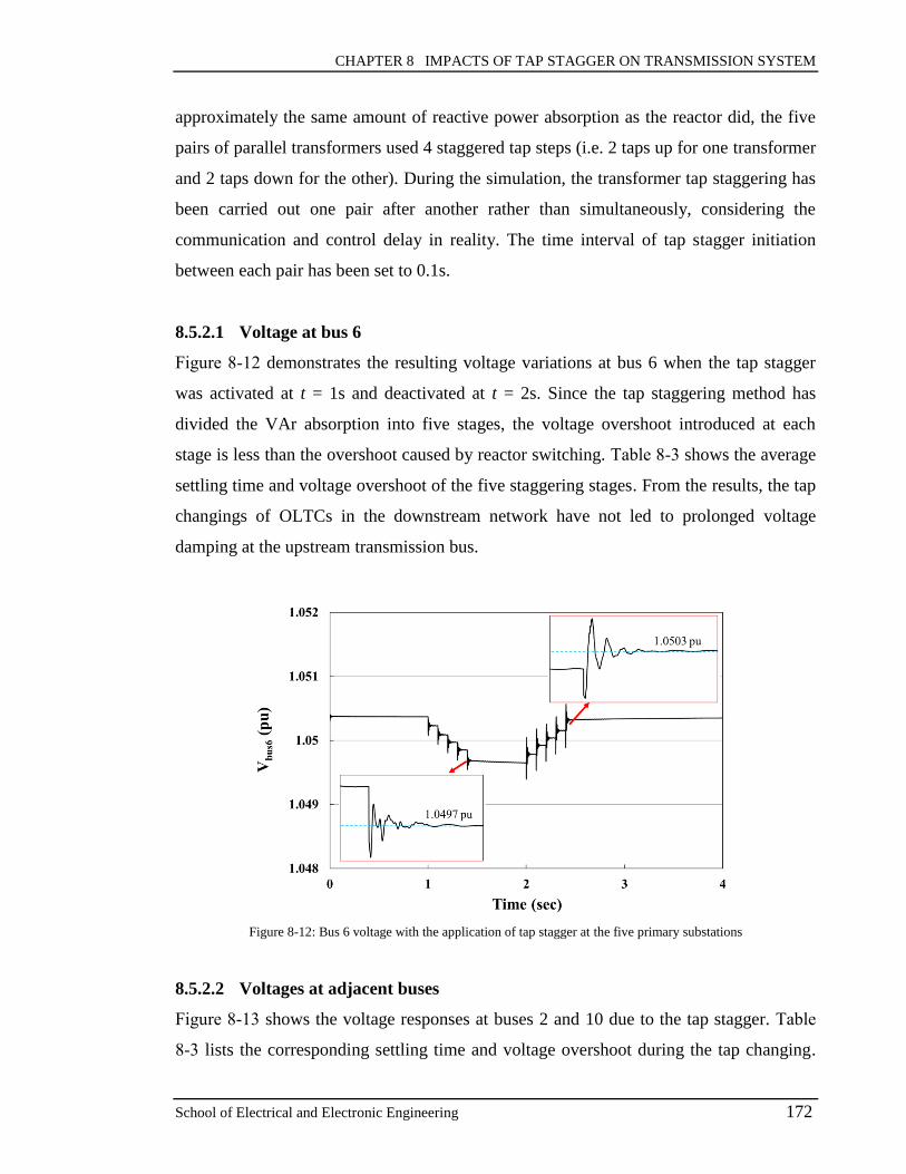
CHAPTER 8 IMPACTS OF TAP STAGGER ON TRANSMISSION SYSTEM
School of Electrical and Electronic Engineering 172
approximately the same amount of reactive power absorption as the reactor did, the five
pairs of parallel transformers used 4 staggered tap steps (i.e. 2 taps up for one transformer
and 2 taps down for the other). During the simulation, the transformer tap staggering has
been carried out one pair after another rather than simultaneously, considering the
communication and control delay in reality. The time interval of tap stagger initiation
between each pair has been set to 0.1s.
8.5.2.1 Voltage at bus 6
Figure 8-12 demonstrates the resulting voltage variations at bus 6 when the tap stagger
was activated at t = 1s and deactivated at t = 2s. Since the tap staggering method has
divided the VAr absorption into five stages, the voltage overshoot introduced at each
stage is less than the overshoot caused by reactor switching. Table 8-3 shows the average
settling time and voltage overshoot of the five staggering stages. From the results, the tap
changings of OLTCs in the downstream network have not led to prolonged voltage
damping at the upstream transmission bus.
Figure 8-12: Bus 6 voltage with the application of tap stagger at the five primary substations
8.5.2.2 Voltages at adjacent buses
Figure 8-13 shows the voltage responses at buses 2 and 10 due to the tap stagger. Table
8-3 lists the corresponding settling time and voltage overshoot during the tap changing.

CHAPTER 8 IMPACTS OF TAP STAGGER ON TRANSMISSION SYSTEM
School of Electrical and Electronic Engineering 173
Compared with the use of a reactor, the tap staggering method has significantly reduced
the settling time (e.g. by around 90%). In addition, the introduced voltage overshoots by
tap stagger are less than the overshoots of reactor switching, especially on bus 6 where
the VAr compensation methods are applied. Note that for both methods, the transient
voltage overshoots at the three buses are small since the amount of reactive power
compensation is not significant, i.e. only around 1 MVAr. However, the studies have
demonstrated that the use of tap stagger can reduce the voltage overshoots during the
switching transient states.
Figure 8-13: Buses 2 & 10 voltages with the application of tap stagger at the five primary substations
Table 8-3: Transient voltage responses with transformer tap staggering
Staggering activated Staggering deactivated
Settling time
(s)a
Overshoot
(%)a
Settling time
(s)a
Overshoot
(%)a
Bus 6 0.093 0.010 0.076 0.024
Bus 2 0.084 0.008 0.052 0.009
Bus 10 0.070 0.007 0.047 0.018
a. Based on the average value of the five tap staggering stages.
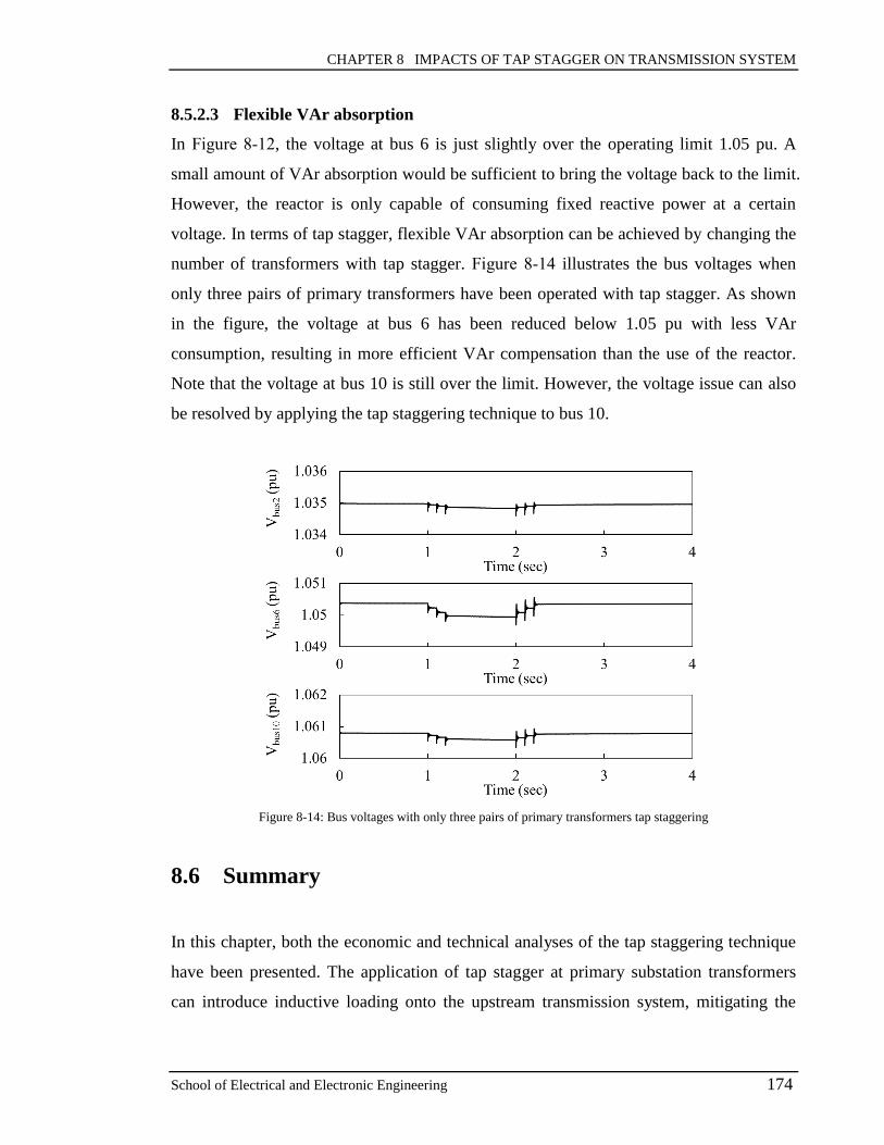
CHAPTER 8 IMPACTS OF TAP STAGGER ON TRANSMISSION SYSTEM
School of Electrical and Electronic Engineering 174
8.5.2.3 Flexible VAr absorption
In Figure 8-12, the voltage at bus 6 is just slightly over the operating limit 1.05 pu. A
small amount of VAr absorption would be sufficient to bring the voltage back to the limit.
However, the reactor is only capable of consuming fixed reactive power at a certain
voltage. In terms of tap stagger, flexible VAr absorption can be achieved by changing the
number of transformers with tap stagger. Figure 8-14 illustrates the bus voltages when
only three pairs of primary transformers have been operated with tap stagger. As shown
in the figure, the voltage at bus 6 has been reduced below 1.05 pu with less VAr
consumption, resulting in more efficient VAr compensation than the use of the reactor.
Note that the voltage at bus 10 is still over the limit. However, the voltage issue can also
be resolved by applying the tap staggering technique to bus 10.
Figure 8-14: Bus voltages with only three pairs of primary transformers tap staggering
8.6 Summary
In this chapter, both the economic and technical analyses of the tap staggering technique
have been presented. The application of tap stagger at primary substation transformers
can introduce inductive loading onto the upstream transmission system, mitigating the

CHAPTER 8 IMPACTS OF TAP STAGGER ON TRANSMISSION SYSTEM
School of Electrical and Electronic Engineering 175
high voltages during periods of low demand. The IEEE RTS system has been modelled to
compare the economic and technical impacts of using the tap staggering technique and
shunt reactors.
In the economic studies, as the use of tap stagger will slightly increase the active demand,
more power will need to be generated to balance the power flow. The TSO may need to
compensate the generators in order to produce extra power. However, the
implementation of tap stagger does not require additional capital investments due to the
utilisation of existing assets. Therefore, for the bus with only occasional high voltage
issues, results indicate that the tap staggering technique is more cost-effective than the
use of reactors. In the system with more frequent voltage violations, a combined method
of applying tap stagger and reactor together can be used to reduce the VAr compensation
costs, resulting in the deferment of high-cost network reinforcements.
In terms of the transient studies, voltage spikes would be introduced at the transmission
buses due to reactor switching. The tap staggering method has been adopted to reduce the
settling time and overshoots of the transient voltages. The use of many distributed
transformers can divide the VAr absorption into several small steps, reducing the overall
dynamic impacts on the transmission system. In addition, the tap staggering method can
provide a flexible reactive power absorption service according to the transmission grid
VAr requirement.
CHAPTER 9 CONCLUSIONS
School of Electrical and Electronic Engineering 176
CHAPTER 9
9 CONCLUSIONS
This chapter summarises the research studies and discusses possible future work plans.
9.1 Conclusions
The thesis first introduced the background of power system voltage and reactive power
control. In recent years, high voltage situations under low demand conditions have been
increasing in the UK transmission system. The main reasons include the development of
underground cables in transmission and distribution networks and the decommissioning
of coal generators in specific areas. In addition, during periods of low demand, National
Grid has observed low reactive power demand or even reactive power injection at several
GSPs. In some cases, reactive power has been exported from the distribution networks to
the transmission system.
The exact cause of this declining trend of reactive power demand during minimum load
periods is still uncertain. The development of underground cables in distribution
networks, the use of more energy-efficient household appliances and the impact of DGs
are some of the possible factors affecting the system VAr demand. On the other hand, to
comply with the forthcoming European Demand Connection Code, distribution networks
should be able to maintain a limited range of reactive power consumption at GSPs.
Therefore, considering the VAr management challenges from both the transmission and
distribution sides, this study aims to develop a cost-effective means of utilising
distribution networks to provide reactive power absorption services for transmission
systems.
Critical reviews of existing Volt/VAr control techniques for both transmission and
distribution systems have been carried out. From the literature, generating units and VAr
compensation devices are commonly used to produce or absorb the reactive power in

CHAPTER 9 CONCLUSIONS
School of Electrical and Electronic Engineering 177
transmission systems. However, with the presence of large-scale intermittent renewable
resources nowadays, voltage problems could become more dynamic and may occur in
different time periods or different regions. The placement and tuning of numbers of
compensation devices at different locations will be challenging for the system operators.
The associated costs will also be high if several devices need to be placed at various
locations in the system. Some studies have demonstrated the benefits of using many,
small and distributed SVCs located at distribution buses to provide reactive power service
for the transmission system. Based on this concept, a new reactive power management
approach to reduce reactive power surplus in the transmission system has been proposed
in this thesis.
The proposed method utilises the existing parallel transformers in distribution networks,
to provide reactive power absorption services for transmission systems during periods of
low demand. The operation of two parallel transformers in different tap positions, i.e.
with staggered taps, will introduce a circulating current around the pair. Due to the
transformer inductance, the circulating current will draw more reactive power from the
upstream network. For each pair, the difference in tap positions should be limited within
a small range to prevent the transformer from overloading and to maintain transformer
secondary voltages. The aggregated VAr absorption from many pairs of parallel
transformers could be used to mitigate the high voltages in the upstream network. In this
research work, the proposed tap staggering method has been applied to the primary
substation transformers, which have OLTCs installed. However, conceptually the tap
staggering technique may be adopted at different voltage levels where there are
transformers operating in parallel.
The ultimate goal of the proposed tap staggering method is to establish a new reactive
power ancillary service, which allows distribution networks to use their existing parallel
transformers to absorb the temporary VAr surplus. The proposed method may be
considered as a smart grid tool to support the reactive power management of the
transmission system. This research project has carried out the essential investigations,
including the feasibility, control and benefit analyses. The major contributions in the

CHAPTER 9 CONCLUSIONS
School of Electrical and Electronic Engineering 178
thesis can be concluded as:
Assessment of the VAr absorption capability of a real UK HV distribution
network with the tap staggering technique. The results have confirmed that the
method has the potential to increase the reactive power demand drawn from the
transmission grid.
Design of an optimal control approach based on GA to coordinate the tap
staggering operation of multiple pairs of parallel transformers. An objective
function has been proposed considering the minimisation of the introduced
power loss as well as the number of tap switching operations.
Comparison of the GA-based tap stagger control approach with two alternative
methods, i.e. the rule-based control scheme and the branch-and-bound method.
Comparison of the impacts of the tap staggering technique and the use of shunt
reactors on transmission systems, in terms of economic cost and dynamic
performance. The results have demonstrated that the tap staggering technique
has economic advantages and can reduce voltage overshoots during the
transient states.
The details of each contribution are summarised as follows.
1) Network Reactive Power Absorption Capability Assessment
To investigate the feasibility of using the tap staggering technique to provide a reactive
power service, network VAr absorption capability studies have been carried out. The
studies are based on the off-line load flow analysis of a real UK HV distribution system
model. The model consists of the networks from the 132kV GSPs down to the 33kV
primary substations. The tap staggering method has been applied to the parallel
transformers at the primary substations. The individual primary substation study
demonstrates that the VAr absorption and power loss of the parallel transformers will
increase quadratically with the number of staggered taps. By applying the tap stagger to
multiple primary substations and using the curve fitting method, the study estimates a
maximum absorption of 1.87 MVAr/substation could be observed at the GSP side.

CHAPTER 9 CONCLUSIONS
School of Electrical and Electronic Engineering 179
However in practice, due to the variations in network demands, the initial OLTC position
may not be at or near the nominal position, resulting in less headroom for the tap stagger.
In addition, the large tap difference may lead to transformer overload. Therefore, a more
conservative study has been carried out considering transformers with only 4 staggered
taps. The results indicate an average VAr absorption of 0.24 MVAr/substation. If each
distribution network can provide a certain amount of VAr absorption, the transmission
system can utilise these inductive reactive power to mitigate the high voltages for some
temporary periods.
2) Tap Stagger Optimal Control based on GA
The thesis has also proposed an optimal control approach for the tap staggering operation.
If the upstream transmission grid requires a specific reactive power to be consumed
during periods of low demand, the distribution system should be able to decide how many
parallel transformers and staggered taps will be used in order to meet the requirement.
The objective function has been defined for the tap stagger control problem, and it has
been solved using the genetic algorithm. The objective is to find an optimal dispatch for
the OLTC tap positions, which minimises the network loss and the number of switching
operations introduced when providing the VAr absorption service. The objective is
subject to the constraints of the VAr absorption error, the OLTC operating ranges and the
permitted staggered taps.
The GA-based tap stagger control method has been applied to a simplified 102-bus
distribution network. With a given VAr requirement, the GA approach can find an
optimal solution that minimises the introduced network loss and the number of tap
switching operations while satisfying the operating constraints. Statistical studies have
been carried out to analyse the accuracy of the VAr absorption provided through the GA
method. The results confirm that the developed GA algorithm is capable of providing the
VAr absorption within the predefined tolerance under different system requirements.
In addition, the GA-based control approach has been investigated using different load
models. The results indicate that the algorithm will return solutions with slightly more tap

CHAPTER 9 CONCLUSIONS
School of Electrical and Electronic Engineering 180
switching operations if the network load is more sensitive to the voltage changes. This is
because, when applying the tap staggering technique, the line voltage drops between the
132kV and 33kV networks will increase. The voltages at the HV and LV sides of the
primary substations will decrease as well, resulting in lower load demands. The reduction
in reactive load demands will counteract the increase in reactive power flow caused by
the tap stagger. To provide the same VAr absorption at the GSP, the control algorithm
has to use more staggered taps to increase the transformer VAr absorption. However, the
changes in the number of tap operations due to different load models are not significant,
i.e. generally within four tap operations. The GA approach has also been tested with
varying load demands, i.e. over a 24-hour period. The result indicates that during periods
of high demand, the network can provide the VAr absorption using fewer tap operations
since the reactive power consumption of lines (due to the tap stagger) increases.
3) Comparison of GA with Rule-Based and Branch-and-Bound
The GA-based tap stagger control approach has been compared with two alternative
solution methods, i.e. the rule-based control scheme and the branch-and-bound algorithm.
The latter two methods have utilised the information of distribution network VAr
absorption capability (i.e. expressed as a sensitivity matrix). To apply the branch-and-
bound method, the tap stagger control problem has been linearised. The three methods
have been investigated with different control settings. The results show that the rule-
based approach provides the fastest control while it does not consider the minimisation of
power losses. For a small system, the branch-and-bound method has a faster convergence
speed than the GA approach. However, due to linearisation errors, the branch-and-bound
method may return solutions that do not actually provide the VAr absorption within the
tolerance. In contrast, the GA approach can produce the most accurate VAr absorption
according to the system requirement. In addition, for a larger distribution system (i.e. the
222-bus distribution network), the average computation time of the GA approach
becomes faster than the branch-and-bound method as the search space of the branch-and-
bound algorithm has increased significantly. Note that, both the rule-based and the
branch-and-bound methods can only be applied to radial distribution networks whereas
the GA approach can also be used for meshed networks.

CHAPTER 9 CONCLUSIONS
School of Electrical and Electronic Engineering 181
4) Impacts of Tap Stagger on Transmission System
Finally, both the economic and technical effects of the tap staggering method on the
transmission system have been discussed and compared with the use of shunt reactors. In
the economic studies, the cost for the TSO to apply the tap staggering technique consists
of the payments for generators as well as DNOs. As the use of tap stagger will slightly
increase the active demand, more power will need to be generated to balance the power
flow. The TSO may need to compensate the generators in order to produce extra power.
However, the implementation of tap stagger does not require additional capital
investments. The TSO only needs to pay the DNOs for providing the reactive power
ancillary services. Therefore, considering these two factors, studies indicate that the tap
staggering technique is more cost-effective than the use of reactors at the bus with only
occasional high voltage issues. In the system with more frequent voltage violations, a
combined method of applying tap stagger and reactor together can be used to reduce the
VAr compensation costs. Consequently, the use of tap stagger may defer the
reinforcements of higher rating reactors or other VAr compensators.
In terms of the transient studies, voltage spikes would be introduced at the transmission
buses due to the reactor switching. The tap staggering method has been adopted to reduce
the settling time and overshoots of the transient voltages. The use of many distributed
transformers can divide the VAr absorption into several small steps, reducing the overall
dynamic impacts on the transmission system. In addition, the tap staggering method can
provide flexible (or adjustable) reactive power absorption according to the transmission
grid VAr requirement.
9.2 Suggestions for Future Work
This research project has concentrated on the necessary investigations of the feasibility,
implementation and effectiveness of the tap staggering technique. Further studies can be
carried out to improve some aspects of the proposed tap staggering method and to design
a real-time system for implementing tap stagger optimal control.

CHAPTER 9 CONCLUSIONS
School of Electrical and Electronic Engineering 182
Load profiles
For the 24-hour optimisation studies presented in the thesis, a typical daily load profile
from literature has been used and both active and reactive demands share the same profile.
However, the CLASS project [123] has been undertaking the demand monitoring of real
UK primary substations and the measurements obtained can be used to establish more
representative load profiles. Further optimisation results can therefore be carried out by
adopting separate load profiles for P and Q loads.
Validation of reactive power absorption
This research work has used load flow simulations to investigate the transformer and
network VAr absorption capability with tap stagger. Several site trials of the tap
staggering technique on real UK primary substations are currently in progress. The
measurements taken at the substations and GSPs will be used to validate the VAr
absorption capability estimated by simulations.
On-line tap stagger control
The proposed GA-based tap stagger control method has been tested with off-line studies.
To further investigate the tap stagger control, a real-time closed-loop system can be
developed. Figure 9-1 illustrates the real-time implementation of the tap stagger control.
Distribution
Network Model
in RTDS
Real-time
Measurements
State
Estimation
GA-based
Optimization
Tap stagger
Other VAr compensators
Figure 9-1: Real-time implementation of the tap stagger optimal control
CHAPTER 9 CONCLUSIONS
School of Electrical and Electronic Engineering 183
First, a distribution network will be modelled using the Real Time Digital Simulator
(RTDS) to generate real-time measurements. Since distribution networks usually lack
real-time monitoring, state estimation will be developed to calculate and observe the
voltage states across the network. According to the estimated voltages, the GA-based
solution procedure will then be performed to determine the optimal tap positions for the
tap stagger. In addition, the optimisation algorithm will consider the coordination with
other existing VAr compensators in the network, such as shunt reactors and capacitor
banks. The coordinated VAr control system is expected to provide a fast and stable
reactive power service to the upstream transmission system under varying generation and
demand conditions.

REFERENCES
School of Electrical and Electronic Engineering 184
REFERENCES
[1] IPCC, "Managing the risks of extreme events and disasters to advance climate
change adaptation," Working Groups I & II, Intergovernmental Panel on Climate
Change, Cambridge University Press, Cambridge, UK, and New York, NY, USA,
2012.
[2] IPCC, "Climate change 2013: the physical science basis," Working Groups I,
Intergovernmental Panel on Climate Change, Cambridge University Press,
Cambridge, UK, and New York, NY, USA, 2013.
[3] Commission of the European Communities, "20 20 by 2020: Europe's climate
change opportunity," COM (2008) 30 final, Brussels, Jan. 2008.
[4] UK Parliament, "Climate Change Act 2008," The Stationery Office Limited,
London, 2008.
[5] Committee on Climate Change, "Meeting carbon budgets – 2014 progress report
to Parliament," London, Jul. 2014. [Online]. Available:
http://www.theccc.org.uk/publication/meeting-carbon-budgets-2014-progress-
report-to-parliament/
[6] UK Department of Energy & Climate Change, "Digest of United Kingdom energy
statistics 2014," National Statistics Publication, The Stationery Office Limited,
London, 2014, ISBN: 9780115155307.
[7] UK Department of Energy & Climate Change, "Planning our electric future: a
White Paper for secure, affordable and low-carbon electricity," The Stationery
Office Limited, London, 2011, ISBN: 9780101809924.
[8] N. Jenkins, R. Allan, P. Crossley, D. Kirschen, and G. Strbac, Embedded
Generation, IEE Power and Energy Series 31, The Institution of Electrical
Engineers, London, 2000, pp. 1-19.
[9] H. L. Willis and W. G. Scott, Distributed Power Generation: Planning and
Evaluation, Power Engineering 10, Marcel Dekker, New York, 2000, pp. 7-11.
[10] N. Jenkins, J. B. Ekanayake, and G. Strbac, Distributed Generation, Renewable
Energy Series 1, The Institution of Electrical Engineers, London, 2010, pp. 6-12,
64-66.
[11] I. Richardson, M. Thomson, D. Infield, and C. Clifford, "Domestic electricity use:
A high-resolution energy demand model," Energy and Buildings, vol. 42, no. 10,
pp. 1878-1887, Oct. 2010.
[12] T. Masuta and A. Yokoyama, "Supplementary load frequency control by use of a
number of both electric vehicles and heat pump water heaters," IEEE
Transactions on Smart Grid, vol. 3, no. 3, pp. 1253-1262, Sep. 2012.
[13] J. Machowski, J. W. Bialek, and J. R. Bumby, Power System Dynamics: Stability
and Control, 2nd ed., John Wiley & Sons, 2008, pp. 35-36.
[14] UK Energy Networks Association (ENA), "A guide for connecting generation to
the distribution network that falls under G59/3," Distributed Generation
Connection Guide, Jun. 2014. [Online]. Available:
http://www.energynetworks.org/electricity/engineering/distributed-
generation/distributed-generation.html
REFERENCES
School of Electrical and Electronic Engineering 185
[15] UK Statutory Instruments, "The electricity safety, quality and continuity
regulations 2002," PART VII, The Stationery Office Limited, London, 2002,
ISBN: 0110429206.
[16] T. J. E. Miller, Reactive Power Control in Electric Systems, John Wiley & Sons,
New York, 1982, pp. 13-18, 353-361.
[17] B. K. Johnson, J. M. Appikonda, and G. Venkataramanan, "Reactive
compensation needs for superconducting transmission systems," IEEE
Transactions On Applied Superconductivity, vol. 19, no. 3, pp. 2066-2069, Jun.
2009.
[18] P. Kundur, Power System Stability and Control, The EPRI Power System
Engineering Series, McGraw-Hill, 1994, pp. 627-687.
[19] M. A. Laughton and D. F. Warne, Electrical Engineer's Reference Book, 16th ed.,
Newnes, Oxford, 2003, pp. 41/1-41/40.
[20] C. R. Bayliss and B. J. Hardy, Transmission and Distribution Electrical
Engineering, 3rd ed., Newnes, Oxford, 2007, pp. 991-994.
[21] M. Thomson, "Automatic voltage control relays and embedded generation. I,"
Power Engineering Journal, vol. 14, no. 2, pp. 71-76, Apr. 2000.
[22] P. N. Vovos, A. E. Kiprakis, A. R. Wallace, and G. P. Harrison, "Centralised and
distributed voltage control: Impact on distributed generation penetration," IEEE
Transactions on Power Systems, vol. 22, no. 1, pp. 476-483, Feb. 2007.
[23] J. A. P. Lopes, N. Hatziargyriou, J. Mutale, P. Djapic, and N. Jenkins,
"Integrating distributed generation into electric power systems: A review of
drivers, challenges and opportunities," Electric Power Systems Research, vol. 77,
no. 9, pp. 1189-1203, Jul. 2007.
[24] C. L. Masters, "Voltage rise: the big issue when connecting embedded generation
to long 11 kV overhead lines," Power Engineering Journal, vol. 16, no. 1, pp. 5-12, Feb. 2002.
[25] National Grid, "Electricity Ten Year Statement 2012," pp. 221-223, Nov. 2012.
[Online]. Available: http://www2.nationalgrid.com/UK/Industry-
information/Future-of-Energy/Electricity-ten-year-statement/
[26] National Grid, "Electricity Ten Year Statement 2013," pp. 207-208, 2013.
[Online]. Available: http://www2.nationalgrid.com/UK/Industry-
information/Future-of-Energy/Electricity-ten-year-statement/
[27] W. Wiechowski and P. B. Eriksen, "Selected studies on offshore wind farm cable
connections - challenges and experience of the Danish TSO," IEEE Power and
Energy Society General Meeting, Pittsburgh, Jul. 2008.
[28] S. Zhang, S. Jiang, X. Lu, B. Ge, and F. Z. Peng, "Resonance issues and damping
techniques for grid-connected inverters with long transmission cable," IEEE
Transactions on Power Electronics, vol. 29, no. 1, pp. 110-120, Jan. 2014.
[29] T. Zhang, L. Sun, and Y. Zhang, "Study on switching overvoltage in off-shore
wind farms," IEEE Transactions on Applied Superconductivity, vol. 24, no. 5, pp.
1-5, Oct. 2014.
[30] C. Kaloudas, L. Ochoa, B. Marshall, and S. Majithia, "Initial assessment of
reactive power exchanges at UK grid supply points," CIRED Workshop 2014,
Rome, Jun. 2014.
REFERENCES
School of Electrical and Electronic Engineering 186
[31] H. Amarís, M. Alonso, and C. A. Ortega, Reactive Power Management of Power
Networks with Wind Generation, Lecture Notes in Energy 5, Springer, London,
2013, pp. 77-95.
[32] National Grid, "National electricity transmission system performance report 2011-
2012," Sep. 2012. [Online]. Available:
http://www2.nationalgrid.com/UK/Industry-information/Electricity-transmission-
operational-data/Report-explorer/Performance-Reports/
[33] M. Constantin, M. Eremia, and L. Toma, "Comparative analysis between
conventional voltage control using reactors and continuous voltage control using
TCR in the Romanian transmission grid," IEEE PowerTech (POWERTECH),
Grenoble, Jun. 2013.
[34] F. B. Alhasawi and J. V. Milanovic, "Techno-economic contribution of FACTS
devices to the operation of power systems with high level of wind power
integration," IEEE Transactions on Power Systems, vol. 27, no. 3, pp. 1414-1421,
Aug. 2012.
[35] European Network of Transmission System Operators for Electricity (ENTSO-E),
"Network Code on Demand Connection," Dec. 2012. [Online]. Available:
https://www.entsoe.eu/major-projects/network-code-development/demand-
connection/Pages/default.aspx
[36] E. Lakervi and E. J. Holmes, Electricity distribution network design, 2nd ed., IEE
Power Engineering Series 21, Peter Peregrinus, London, 1995, pp. 9-17, 252-271.
[37] B. M. Weedy, B. J. Cory, N. Jenkins, J. B. Ekanayake, and G. Strbac, Electric
Power Systems, 5th ed., John Wiley & Sons, Chichester, 2012, pp. 100-103, 180-
183.
[38] H. Vu, P. Pruvot, C. Launay, and Y. Harmand, "An improved voltage control on
large-scale power system," IEEE Transactions on Power Systems, vol. 11, no. 3,
pp. 1295-1303, Aug. 1996.
[39] T. V. Cutsem and C. Vournas, Voltage Stability of Electric Power Systems, Power
Electronics and Power Systems Series, Springer, New York, 1998, pp. 67-89.
[40] J. D. Hurley, L. N. Bize, and C. R. Mummert, "The adverse effects of excitation
system VAr and power factor controllers," IEEE Transactions on Energy
Conversion, vol. 14, no. 4, pp. 1636-1645, Dec. 1999.
[41] J. P. Paul, J. Y. Leost, and J. M. Tesseron, "Survey of the secondary voltage
control in France: present realization and investigations," IEEE Transactions on
Power Systems, vol. 2, no. 2, pp. 505-511, May 1987.
[42] P. Lagonotte, J. C. Sabonnadiere, J. Y. Leost, and J. P. Paul, "Structural analysis
of the electrical system: application to secondary voltage control in France," IEEE
Transactions on Power Systems, vol. 4, no. 2, pp. 479-486, May 1989.
[43] S. Corsi, P. Marannino, N. Losignore, G. Moreschini, and G. Piccini,
"Coordination between the reactive power scheduling function and the
hierarchical voltage control of the EHV ENEL system," IEEE Transactions on
Power Systems, vol. 10, no. 2, pp. 686-694, May 1995.
[44] A. Berizzi, P. Marannino, M. Merlo, M. Pozzi, and F. Zanellini, "Steady-state and
dynamic approaches for the evaluation of loadability margins in the presence of
secondary voltage regulation," IEEE Transactions on Power Systems, vol. 19, no.
2, pp. 1048-1057, May 2004.

REFERENCES
School of Electrical and Electronic Engineering 187
[45] J. L. Sancha, J. L. Fernandez, A. Cortes, and J. T. Abarca, "Secondary voltage
control: analysis, solutions and simulation results for the Spanish transmission
system," IEEE Transactions on Power Systems, vol. 11, no. 2, pp. 630-638, May
1996.
[46] A. Conejo and M. J. Aguilar, "Secondary voltage control: nonlinear selection of
pilot buses, design of an optimal control law, and simulation results," IEE
Proceedings of Generation, Transmission and Distribution, vol. 145, no. 1, pp.
77-81, Jan. 1998.
[47] H. F. Wang, "Multi-agent co-ordination for the secondary voltage control in
power-system contingencies," IEE Proceedings of Generation, Transmission and
Distribution, vol. 148, no. 1, pp. 61-66, Jan. 2001.
[48] W. Hai Feng, H. Li, and H. Chen, "Coordinated secondary voltage control to
eliminate voltage violations in power system contingencies," IEEE Transactions
on Power Systems, vol. 18, no. 2, pp. 588-595, May 2003.
[49] H. Mehrjerdi, S. Lefebvre, M. Saad, and D. Asber, "Coordinated control strategy
considering effect of neighborhood compensation for voltage improvement in
transmission systems," IEEE Transactions on Power Systems, vol. 28, no. 4, pp.
4507-4515, Nov. 2013.
[50] S. Corsi, M. Pozzi, C. Sabelli, and A. Serrani, "The coordinated automatic voltage
control of the Italian transmission grid-part I: reasons of the choice and overview
of the consolidated hierarchical system," IEEE Transactions on Power Systems,
vol. 19, no. 4, pp. 1723-1732, Nov. 2004.
[51] S. Corsi, M. Pozzi, M. Sforna, and G. Dell'Olio, "The coordinated automatic
voltage control of the Italian transmission grid-part II: control apparatuses and
field performance of the consolidated hierarchical system," IEEE Transactions on
Power Systems, vol. 19, no. 4, pp. 1733-1741, Nov. 2004.
[52] A. S. Pabla, Electric Power Distribution, McGraw-Hill, New York, 2005, pp.
168-177.
[53] T. Gönen, Electric Power Distribution System Engineering, 2nd ed., CRC Press,
Boca Raton, 2008, pp. 441-484.
[54] J. H. Choi and J. C. Kim, "The online voltage control of ULTC transformer for
distribution voltage regulation," International Journal Of Electrical Power &
Energy Systems, vol. 23, no. 2, pp. 91-98, Feb. 2001.
[55] M. E. Baran and M. Y. Hsu, "Volt/Var control at distribution substations," IEEE
Transactions on Power Systems, vol. 14, no. 1, pp. 312-318, Feb. 1999.
[56] W. H. Kersting, Distribution System Modeling and Analysis, 3rd ed., The Electric
Power Engineering Series, CRC Press, Boca Raton, 2012, pp. 179-233.
[57] S. N. Liew and G. Strbac, "Maximising penetration of wind generation in existing
distribution networks," IEE Proceedings of Generation, Transmission and
Distribution, vol. 149, no. 3, pp. 256-262, May 2002.
[58] M. Fila, G. A. Taylor, J. Hiscock, M. R. Irving, and P. Lang, "Flexible voltage
control to support distributed generation in distribution networks," 43rd
International Universities Power Engineering Conference, Padova, Sep. 2008.
[59] C. Gao and M. A. Redfern, "A review of voltage control techniques of networks
with distributed generations using on-load tap changer transformers," 45th
International Universities Power Engineering Conference, Cardiff, Sep. 2010.
REFERENCES
School of Electrical and Electronic Engineering 188
[60] R. El-Feres and H. Li, "Development of adaptive voltage controller for active
distribution network operation with distributed generation," International
Conference on Advanced Power System Automation and Protection (APAP), Jeju,
Apr. 2007.
[61] J. J. Gainger and W. D. Stevenson, Power System Analysis, McGraw-Hill, 1994,
pp. 642-655.
[62] A. J. Wood and B. F. Wollenberg, Power Generation, Operation, and Control,
2nd ed., John Wiley & Sons, New York, 1996, pp. 458-508.
[63] K. Li, "State estimation for power distribution system and measurement impacts,"
IEEE Transactions on Power Systems, vol. 11, no. 2, pp. 911-916, May 1996.
[64] C. M. Hird, H. Leite, N. Jenkins, and H. Li, "Network voltage controller for
distributed generation," IEE Proceedings of Generation, Transmission and
Distribution, vol. 151, no. 2, pp. 150-156, Mar. 2004.
[65] S. S. Baghsorkhi and I. A. Hiskens, "Impact of wind power variability on sub-
transmission networks," IEEE Power and Energy Society General Meeting, San
Diego, Jul. 2012.
[66] S. N. Salih, C. Peiyuan, and O. Carlson, "The effect of wind power integration on
the frequency of tap changes of a substation transformer," IEEE Transactions on
Power Systems, vol. 28, no. 4, pp. 4320-4327, Nov. 2013.
[67] P. M. S. Carvalho, P. F. Correia, and L. A. F. M. Ferreira, "Distributed reactive
power generation control for voltage rise mitigation in distribution networks,"
IEEE Transactions on Power Systems, vol. 23, no. 2, pp. 766-772, May 2008.
[68] M. E. Moursi, G. Joos, and C. Abbey, "A secondary voltage control strategy for
transmission level interconnection of wind generation," IEEE Transactions On
Power Electronics, vol. 23, no. 3, pp. 1178-1190, May 2008.
[69] A. Ahmidi, X. Guillaud, Y. Besanger, and R. Blanc, "A multilevel approach for
optimal participating of wind farms at reactive power balancing in transmission
power system," IEEE Systems Journal, vol. 6, no. 2, pp. 260-269, Jun. 2012.
[70] N. R. Ullah, K. Bhattacharya, and T. Thiringer, "Wind farms as reactive power
ancillary service providers—technical and economic issues," IEEE Transactions
On Energy Conversion, vol. 24, no. 3, pp. 661-672, Sep. 2009.
[71] Z. Saad-Saoud, M. L. Lisboa, J. B. Ekanayake, N. Jenkins, and G. Strbac,
"Application of STATCOMs to wind farms," IEE Proceedings of Generation,
Transmission and Distribution, vol. 145, no. 5, pp. 511-516, Sep. 1998.
[72] P. Hwang, S. Ahn, Y. Yoon, and S. Moon, "A control method of distributed
generators in smart distribution system considering system loss and voltage,"
CIRED 21st International Conference on Electricity Distribution, Frankfurt, Jun.
2011.
[73] S. Conti, A. Greco, N. Messina, and S. Raiti, "Local voltage regulation in LV
distribution networks with PV distributed generation," International Symposium
on Power Electronics, Electrical Drives, Automation and Motion (SPEEDAM),
Taormina, May 2006.
[74] E. F. Mogos and X. Guillaud, "A voltage regulation system for distributed
generation," IEEE PES Power Systems Conference and Exposition, New York,
Oct. 2004.

REFERENCES
School of Electrical and Electronic Engineering 189
[75] A. A. Al-Ohaly and Z. Elrazaz, "Shunt reactors as counter measure for reactive
power surplus: location and impact on system stability performance," Canadian
Electrical Engineering Journal, vol. 12, no. 2, pp. 85-88, Apr. 1987.
[76] W. Li, S. Pai, M. Kwok, and J. Sun, "Determining rational redundancy of 500-kV
reactors in transmission systems using a probability-based economic analysis
approach: BCTC's practice," IEEE Transactions on Power Systems, vol. 19, no. 1,
pp. 325-329, Feb. 2004.
[77] H. Samet and M. Rashidi, "Coordinated under frequency load and capacitor
shedding for bulk power systems," IET Generation, Transmission and
Distribution, vol. 7, no. 8, pp. 799-812, Aug. 2013.
[78] J. L. Aguero, P. L. Arnera, R. E. B. Lastra, and M. C. Beroqui, "Synchronous
compensators: models verified by tests of automatic voltage regulator, reactive
power control, and voltage joint control," IEEE Transactions on Power Systems,
vol. 21, no. 4, pp. 1798-1807, Nov. 2006.
[79] J. Dixon, L. Moran, J. Rodriguez, and R. Domke, "Reactive power compensation
technologies: state-of-the-art review," Proceedings of the IEEE, vol. 93, no. 12,
pp. 2144-2164, Dec. 2005.
[80] G. Romegialli and H. Beeler, "Reactive compensation problems and concepts of
static compensator control," IEE Proceedings of Generation, Transmission and
Distribution, vol. 128, no. 6, pp. 382-388, Nov. 1981.
[81] R. T. Byerly, D. T. Poznaniak, and E. R. Taylor, "Static reactive compensation for
power transmission systems," IEEE Transactions on Power Apparatus and
Systems, vol. PAS-101, no. 10, pp. 3997-4005, Oct. 1982.
[82] N. Martins, N. J. P. Macedo, L. T. G. Lima, and H. J. C. P. Pinto, "Control
strategies for multiple static VAr compensators in long distance voltage supported
transmission systems," IEEE Transactions on Power Systems, vol. 8, no. 3, pp.
1107-1117, Aug. 1993.
[83] C. Schauder, M. Gernhardt, E. Stacey, T. Lemak, L. Gyugyi, T. W. Cease, et al.,
"Development of a ±100 MVAr static condenser for voltage control of
transmission systems," IEEE Transactions on Power Delivery, vol. 10, no. 3, pp.
1486-1496, Jul. 1995.
[84] B. Singh, R. Saha, A. Chandra, and K. Al-Haddad, "Static synchronous
compensators (STATCOM): a review," IET Power Electronics, vol. 2, no. 4, pp.
297-324, Jul. 2009.
[85] The Union of the Electricity Industry - EURELECTRIC, "Connection Rules for
Generation and Management of Ancillary Services," Brussels, Ref: 2000-130-
0003, May 2000. [Online]. Available:
www.eurelectric.org/Download/Download.aspx?DocumentID=5908
[86] K. Bhattacharya and Z. Jin, "Reactive power as an ancillary service," IEEE
Transactions On Power Systems, vol. 16, no. 2, pp. 294-300, May 2001.
[87] M. De and S. K. Goswami, "Reactive support allocation using improved Y-bus
matrix method," IET Generation, Transmission & Distribution, vol. 5, no. 4, pp.
448-460, Apr. 2011.
[88] C. Vyjayanthi and D. Thukaram, "Evaluation and improvement of generators
reactive power margins in interconnected power systems," IET Generation,
Transmission & Distribution, vol. 5, no. 4, pp. 504-518, Apr. 2011.

REFERENCES
School of Electrical and Electronic Engineering 190
[89] O. Homaee and S. Jadid, "Investigation of synchronous generator in reactive
power market - an accurate view," IET Generation, Transmission & Distribution,
vol. 8, no. 11, pp. 1881-1890, Nov. 2014.
[90] Z. Elrazaz and A. A. Al-Ohaly, "Optimal coordination of shunt reactors to
enhance system performance at light load operation," IEE Proceedings of
Generation, Transmission and Distribution, vol. 140, no. 4, pp. 293-298, Jul.
1993.
[91] D. Porter, G. Strbac, and J. Mutale, "Ancillary service provision from distributed
generation," CIRED 18th International Conference on Electricity Distribution,
Turin, Jun. 2005.
[92] A. Cagnano, E. D. Tuglie, M. Liserre, and R. A. Mastromauro, "Online optimal
reactive power control strategy of PV inverters," IEEE Transactions On Industrial
Electronics, vol. 58, no. 10, pp. 4549-4558, Oct. 2011.
[93] A. C. Rueda-Medina and A. Padilha-Feltrin, "Distributed generators as providers
of reactive power support - a market approach," IEEE Transactions On Power
Systems, vol. 28, no. 1, pp. 490-502, Feb. 2013.
[94] N. Jelani, M. Molinas, and S. Bolognani, "Reactive power ancillary service by
constant power loads in distributed AC systems," IEEE Transactions on Power
Delivery, vol. 28, no. 2, pp. 920-927, Apr. 2013.
[95] N. R. Ullah, T. Thiringer, and D. Karlsson, "Voltage and transient stability
support by wind farms complying with the E.ON Netz grid code," IEEE
Transactions on Power Systems, vol. 22, no. 4, pp. 1647-1656, Nov. 2007.
[96] H. Yoshida, K. Kawata, Y. Fukuyama, S. Takayama, and Y. Nakanishi, "A
particle swarm optimization for reactive power and voltage control considering
voltage security assessment," IEEE Transactions on Power Systems, vol. 15, no. 4,
pp. 1232-1239, Nov. 2000.
[97] L. Furong, J. D. Pilgrim, C. Dabeedin, A. Chebbo, and R. K. Aggarwal, "Genetic
algorithms for optimal reactive power compensation on the national grid system,"
IEEE Transactions on Power Systems, vol. 20, no. 1, pp. 493-500, Feb. 2005.
[98] A. Khorsandi, A. Alimardani, B. Vahidi, and S. H. Hosseinian, "Hybrid shuffled
frog leaping algorithm and Nelder-Mead simplex search for optimal reactive
power dispatch," IET Generation, Transmission and Distribution, vol. 5, no. 2, pp.
249-256, Feb. 2011.
[99] S. Duman, Y. Sonmez, U. Guvenc, and N. Yorukeren, "Optimal reactive power
dispatch using a gravitational search algorithm," IET Generation, Transmission
and Distribution, vol. 6, no. 6, pp. 563-576, Jun. 2012.
[100] C. M. Huang, S. J. Chen, Y. C. Huang, and H. T. Yang, "Comparative study of
evolutionary computation methods for active-reactive power dispatch," IET
Generation, Transmission and Distribution, vol. 6, no. 7, pp. 636-645, Jul. 2012.
[101] H. Liu, L. Jin, J. D. McCalley, R. Kumar, V. Ajjarapu, and N. Elia, "Planning
reconfigurable reactive control for voltage stability limited power systems," IEEE
Transactions On Power Systems, vol. 24, no. 2, pp. 1029-1038, May 2009.
[102] S. Kincic, X. T. Wan, D. T. McGillis, A. Chandra, B. T. Ooi, F. D. Galiana, et al.,
"Voltage support by distributed static VAr systems (SVS)," IEEE Transactions
On Power Delivery, vol. 20, no. 2, pp. 1541-1549, Apr. 2005.

REFERENCES
School of Electrical and Electronic Engineering 191
[103] S. Kincic, B. T. Ooi, D. McGillis, and A. Chandra, "Voltage support of radial
transmission lines by var compensation at distribution buses," IEE Proceedings of
Generation, Transmission and Distribution, vol. 153, no. 1, pp. 51-58, Jan. 2006.
[104] D. Youman, R. Xiaojuan, Z. Changcheng, and Z. Dapu, "A heuristic and
algorithmic combined approach for reactive power optimization with time-
varying load demand in distribution systems," IEEE Transactions on Power
Systems, vol. 17, no. 4, pp. 1068-1072, Nov. 2002.
[105] Z. Hu, X. Wang, H. Chen, and G. A. Taylor, "Volt/VAr control in distribution
systems using a time-interval based approach," IEE Proceedings of Generation,
Transmission and Distribution, vol. 150, no. 5, pp. 548-554, Sep. 2003.
[106] A. Ulinuha, M. A. S. Masoum, and S. Islam, "Hybrid genetic-fuzzy algorithm for
volt/var/total harmonic distortion control of distribution systems with high
penetration of non-linear loads," IET Generation, Transmission and Distribution,
vol. 5, no. 4, pp. 425-439, Apr. 2011.
[107] B. Milosevic and M. Begovic, "Capacitor placement for conservative voltage
reduction on distribution feeders," IEEE Transactions on Power Delivery, vol. 19,
no. 3, pp. 1360-1367, Jul. 2004.
[108] A. Augugliaro, L. Dusonchet, S. Favuzza, and E. R. Sanseverino, "Voltage
regulation and power losses minimization in automated distribution networks by
an evolutionary multiobjective approach," IEEE Transactions on Power Systems,
vol. 19, no. 3, pp. 1516-1527, Aug. 2004.
[109] D. Villacci, G. Bontempi, and A. Vaccaro, "An adaptive local learning-based
methodology for voltage regulation in distribution networks with dispersed
generation," IEEE Transactions on Power Systems, vol. 21, no. 3, pp. 1131-1140,
Aug. 2006.
[110] M. B. Liu, C. A. Canizares, and W. Huang, "Reactive power and voltage control
in distribution systems with limited switching operations," IEEE Transactions on
Power Systems, vol. 24, no. 2, pp. 889-899, May 2009.
[111] F. C. Lu and Y. Y. Hsu, "Reactive power/voltage control in a distribution
substation using dynamic programming," IEE Proceedings of Generation,
Transmission and Distribution, vol. 142, no. 6, pp. 639-645, Nov. 1995.
[112] R. H. Liang and C. K. Cheng, "Dispatch of main transformer ULTC and
capacitors in a distribution system," IEEE Transactions on Power Delivery, vol.
16, no. 4, pp. 625-630, Oct. 2001.
[113] Y. Liu, P. Zhang, and X. Qiu, "Optimal volt/var control in distribution systems,"
International Journal Of Electrical Power & Energy Systems, vol. 24, no. 4, pp.
271-276, May 2002.
[114] J. Y. Park, S. R. Nam, and J. K. Park, "Control of a ULTC considering the
dispatch schedule of capacitors in a distribution system," IEEE Transactions on
Power Systems, vol. 22, no. 2, pp. 755-761, May 2007.
[115] R. H. Liang and Y. S. Wang, "Fuzzy-based reactive power and voltage control in
a distribution system," IEEE Transactions on Power Delivery, vol. 18, no. 2, pp.
610-618, Apr. 2003.
[116] British Standards Institution (BSI), "Voltage characteristics of electricity supplied
by public electricity networks," BS EN 50160:2010, Aug. 2010, ISBN:
9780580741036.
REFERENCES
School of Electrical and Electronic Engineering 192
[117] J. H. Harlow, Electric Power Transformer Engineering, 2nd ed., The Electrical
Engineering Handbook Series, CRC Press, Boca Raton, 2007, pp. 13/1-13/31.
[118] B. O. Brewin, S. C. E. Jupe, M. G. Bartlett, K. T. Jackson, and C. Hanmer, "New
technologies for low voltage distribution networks," IEEE PES Innovative Smart
Grid Technologies (ISGT) European, Manchester, Dec. 2011.
[119] J. D. Glover, M. S. Sarma, and T. J. Overbye, Power System Analysis and Design,
5th, SI ed., Cengage Learning, USA, 2011, pp. 102-140.
[120] M. Thomson, "Automatic voltage control relays and embedded generation. II,"
Power Engineering Journal, vol. 14, no. 3, pp. 93-99, Jun. 2000.
[121] K. Harker, Power System Commissioning and Maintenance Practice, IEE Power
Series 24, London, The Institution of Electrical Engineers, 1998, pp. 123-147.
[122] M. J. Heathcote, The J & P Transformer Book, 13th ed., Newnes, Oxford, 2007,
pp. 470-481.
[123] Electricity North West Limited (ENWL), "Low Carbon Networks Fund
submission from Electricity North West - CLASS," Nov. 2012. [Online].
Available: https://www.ofgem.gov.uk/electricity/distribution-networks/network-
innovation/low-carbon-networks-fund/second-tier-projects/electricity-north-west-
limited
[124] IPSA Power Group, IPSA Power. [Online]. Available: http://www.ipsa-
power.com/
[125] J. O. Rawlings, S. G. Pantula, and D. A. Dickey, Applied Regression Analysis: A
Research Tool, 2nd ed., Springer-Verlag, New York, 1998, pp. 2-16.
[126] S. WEISBERG, Applied Linear Regression, 3rd ed., John Wiley & Sons, New
Jersey, 2005, pp. 19-38.
[127] Electric Power Research Institute, OpenDSS. [Online]. Available:
http://sourceforge.net/projects/electricdss/
[128] R. C. Dugan, "OpenDSS Manual," Electric Power Research Institute, Mar. 2012.
[Online]. Available:
http://sourceforge.net/projects/electricdss/files/?source=navbar
[129] Z. Michalewics, Genetic Algorithms + Data Structures = Evolution Programs,
3rd, Revised and Extended ed., Springer-Verlag, 1996, pp. 11-55.
[130] A. Shukla, R. Tiwari, and R. Kala, Towards Hybrid and Adaptive Computing: A
Perspective, Springer-Verlag, Berlin Heidelberg, 2010, pp. 69-73.
[131] Global Optimization Toolbox, "Genetic Algorithm," MATLAB Documentation
Centre. [Online]. Available: http://www.mathworks.co.uk/help/gads/genetic-
algorithm.html
[132] National Grid Electricity Transmission, "The Grid Code," Balancing Code No.2,
Issue 5 Revision 2, pp. 21-25, Jan. 2013.
[133] IEEE, "Load representation for dynamic performance analysis," IEEE
Transactions on Power Systems, vol. 8, no. 2, pp. 472-482, May 1993.
[134] UKERC Energy Data Centre, "Electricity user load profiles (daily) by profile
class," 1997. [Online]. Available:
http://data.ukedc.rl.ac.uk/browse/edc/Electricity/LoadProfile
[135] L. A. Wolsey, Integer Programming, John Wiley & Sons, Chichester, 1998, pp.
91-107.

REFERENCES
School of Electrical and Electronic Engineering 193
[136] G. B. Dantzig and M. N. Thapa, Linear Programming 2: Theory and Extensions,
Springer-Verlag, New York, 2003, pp. 128-137.
[137] Optimization Toolbox, "Branch and Bound Algorithm," MATLAB
Documentation Centre. [Online]. Available:
http://uk.mathworks.com/help/optim/ug/mixed-integer-linear-programming-
algorithms.html#btv20bd
[138] "The IEEE reliability test system - 1996," IEEE Reliability Test System Task
Force of Applications of Probability Methods Subcommittee, IEEE Transactions
on Power Systems, vol. 14, no. 3, pp. 1010-1020, Aug. 1999.
[139] R. D. Zimmerman, C. E. Murillo-Sánchez, and R. J. Thomas, "MATPOWER:
steady-state operations, planning and analysis tools for power systems research
and education," IEEE Transactions on Power Systems, vol. 26, no. 1, pp. 12-19,
Feb. 2011.
[140] National Grid Electricity Transmission, "The Grid Code," Connection Conditions,
Issue 5 Revision 2, pp. 7-8, Jan. 2013.
[141] National Grid Electricity Transmission, "The Connection and Use of System
Code," Section 4 - Balancing Services, v1.20, Aug. 2014.
[142] PJM, "Transmission expansion advisory committee (TEAC) recommendations to
the PJM board," Oct. 2013. [Online]. Available:
http://www.pjm.com/~/media/committees-
groups/committees/teac/20141111/20141111-board-approval-of-rtep-
whitepaper.ashx
[143] National Grid Electricity Transmission, "Obligatory reactive power service -
default payment rates," Mar. 2015. [Online]. Available:
http://www2.nationalgrid.com/UK/Services/Balancing-services/Reactive-power-
services/Obligatory-Reactive-Power/
[144] DIgSILENT PowerFactory, 2014. [Online]. Available:
http://www.digsilent.de/index.php/products-powerfactory.html
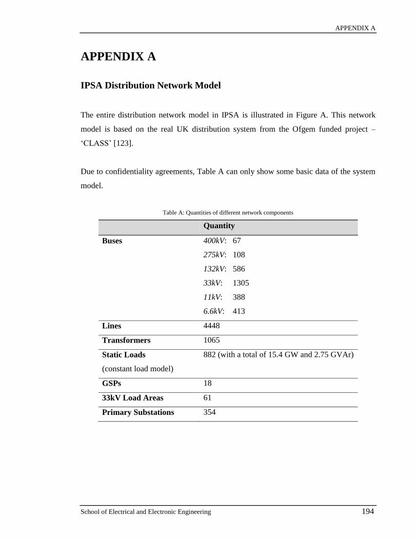
APPENDIX A
School of Electrical and Electronic Engineering 194
APPENDIX A
IPSA Distribution Network Model
The entire distribution network model in IPSA is illustrated in Figure A. This network
model is based on the real UK distribution system from the Ofgem funded project –
‘CLASS’ [123].
Due to confidentiality agreements, Table A can only show some basic data of the system
model.
Table A: Quantities of different network components
Quantity
Buses 400kV: 67
275kV: 108
132kV: 586
33kV: 1305
11kV: 388
6.6kV: 413
Lines 4448
Transformers 1065
Static Loads
(constant load model)
882 (with a total of 15.4 GW and 2.75 GVAr)
GSPs 18
33kV Load Areas 61
Primary Substations 354

APPENDIX A
School of Electrical and Electronic Engineering 195
Grid Infeed
(400 kV & 275 kV)
GSPs (132 kV)
Load Areas (33 kV)
Figure A: Distribution network model simulated in IPSA+ V1.6.8
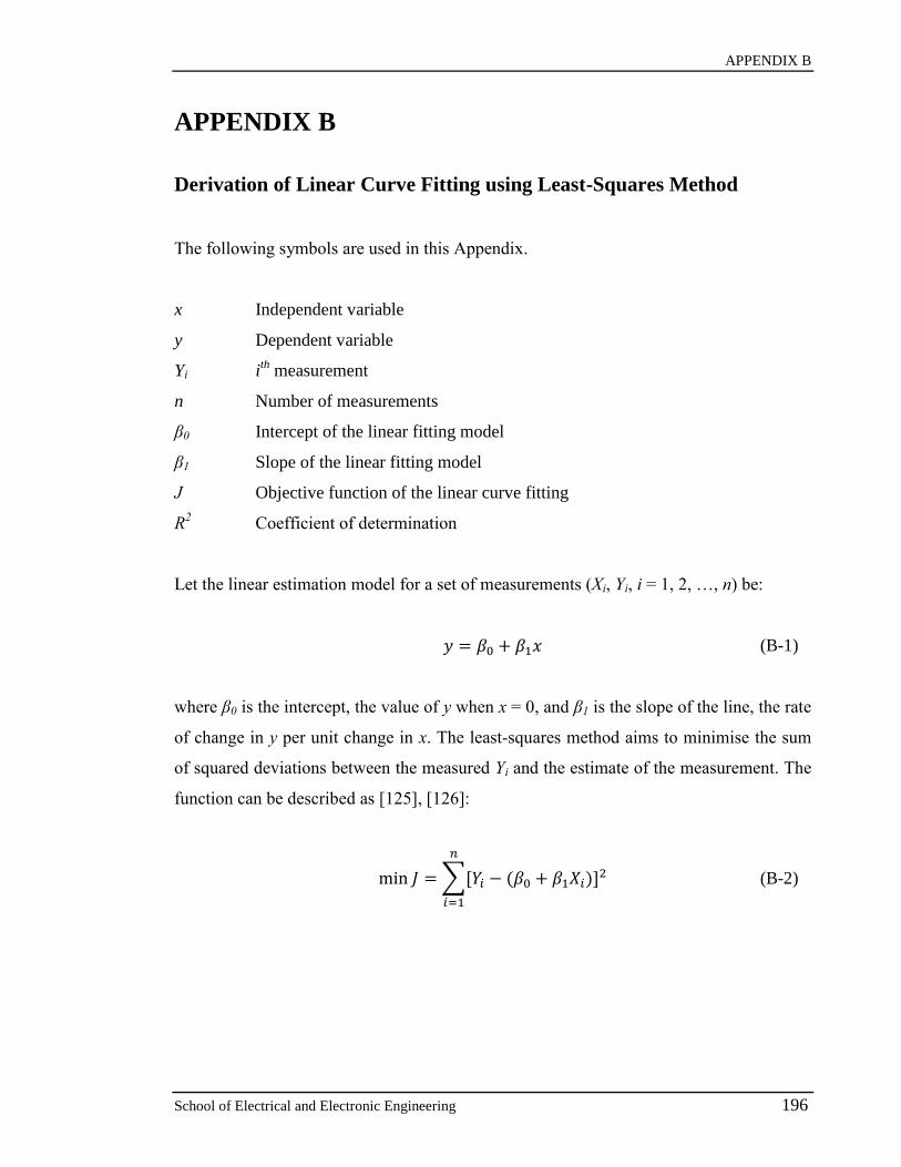
APPENDIX B
School of Electrical and Electronic Engineering 196
APPENDIX B
Derivation of Linear Curve Fitting using Least-Squares Method
The following symbols are used in this Appendix.
x Independent variable
y Dependent variable
Yi ith
measurement
n Number of measurements
β0 Intercept of the linear fitting model
β1 Slope of the linear fitting model
J Objective function of the linear curve fitting
R2 Coefficient of determination
Let the linear estimation model for a set of measurements (Xi, Yi, i = 1, 2, …, n) be:
𝑦 = 𝛽0 + 𝛽1𝑥 (B-1)
where β0 is the intercept, the value of y when x = 0, and β1 is the slope of the line, the rate
of change in y per unit change in x. The least-squares method aims to minimise the sum
of squared deviations between the measured Yi and the estimate of the measurement. The
function can be described as [125], [126]:
min 𝐽 = ∑[𝑌𝑖 − (𝛽0 + 𝛽1𝑋𝑖)]2
𝑛
𝑖=1
(B-2)

APPENDIX B
School of Electrical and Electronic Engineering 197
Taking partial derivatives of Equation (B-2) with respect to β0 and β1:
𝜕𝐽
𝜕𝛽0= −2∑(𝑌𝑖 − 𝛽0 − 𝛽1𝑋𝑖)
𝑛
𝑖=1
(B-3)
𝜕𝐽
𝜕𝛽1= −2∑𝑋𝑖(𝑌𝑖 − 𝛽0 − 𝛽1𝑋𝑖)
𝑛
𝑖=1
(B-4)
The minimum value of J is obtained when both the derivatives are equal to 0. Therefore,
−𝛽0𝑛 − 𝛽1 ∑𝑋𝑖
𝑛
𝑖=1
+ ∑𝑌𝑖
𝑛
𝑖=1
= 0 (B-5)
−𝛽0 ∑𝑋𝑖
𝑛
𝑖=1
− 𝛽1 ∑𝑋𝑖2
𝑛
𝑖=1
+ ∑𝑋𝑖𝑌𝑖
𝑛
𝑖=1
= 0 (B-6)
based on Equations (B-5) and (B-6), the values of β0 and β1 can be calculated as:
𝛽0 = 𝑌 − 𝛽1𝑋 (B-7)
𝛽1 =𝑋𝑌 − 𝑋 ∙ 𝑌
𝑋2 − 𝑋2 (B-8)
where 𝑋 =1
𝑛∑ 𝑋𝑖
𝑛𝑖=1 , 𝑌 =
1
𝑛∑ 𝑌𝑖
𝑛𝑖=1 , 𝑋2 =
1
𝑛∑ 𝑋𝑖
2𝑛𝑖=1 and 𝑋𝑌 =
1
𝑛∑ 𝑋𝑖𝑌𝑖
𝑛𝑖=1 . In order to
indicate how well the measured data fit the linear estimation model, the coefficient of
determination R2 is often used, which can be defined as [125], [126]:
𝑅2 = 1 −∑ [𝑌𝑖 − (𝛽0 + 𝛽1𝑋𝑖)]
2𝑛𝑖=1
∑ (𝑌𝑖 − 𝑌)2𝑛𝑖=1
(B-9)
The coefficient of determination ranges from 0 to 1. An estimated model is most accurate
when the coefficient is at or near 1.

APPENDIX C
School of Electrical and Electronic Engineering 198
APPENDIX C
MATLAB Codes for the GA-Based Tap Stagger Optimisation
Main function
clear;
tic;
%driving OpenDSS using Matlab
[DSSStartOK, DSSObj, DSSText] = DSSStartup;
if DSSStartOK
%Initialization
fstarting=fopen('startingposition.txt');
ftap=fopen('tapchanger.txt');
record=textscan(fstarting,'%*s%*c%*c%*c%*c%f%*[^\n]');
startingpos=cell2mat(record);
%record the MaxTap, MinTap and NumTaps
tap=ones(length(startingpos),3);
i=1;
while ~feof(ftap)
record=textscan(ftap,'%*s%*c%d',1,'delimiter','.'); %record the NO. of transformer
i=record{1};
record=textscan(ftap,'%*s%*c%*c%*c%*c%*c%*c%*c%f%*c%*c%*c%*c%*c%*c%*c%f%*c%*c%*c
%*c%*c%*c%*c%*c%f%*[^\n]',1);
tap(i,:)=cell2mat(record);
record=textscan(ftap,'%s%*[^\n]',1); %skip the next line
end
%change the NumTaps to TapStep(%)
tap(:,3)=round((tap(:,1)-tap(:,2))./tap(:,3)*10000)/100;
%set up the OpenDSS interface variables
currentpath=cd;
DSSText.command=['Compile (' currentpath '\Master.dss)']; %initial network data
DSSCircuit=DSSObj.ActiveCircuit;
DSSSolution=DSSCircuit.Solution;
DSSText.Command='Set Normvmaxpu=1.06';
DSSText.Command='Set Normvminpu=0.94';
DSSText.Command='Set Maxiter=100';
DSSText.Command='Set Maxcontroliter=30';
DSSText.Command='Set tolerance=0.000001';
DSSText.Command='New Energymeter.m1 Transformer.T33 1';
DSSText.Command='New Monitor.PQ_m1 Transformer.T33 2 Mode=1';
%Specify the tested primary transformers (A,B,C,D,E,F,G,H,I,J,K)
testedtrans=[31 30 20 21 23 22 24 25 28 29 26 27 7 6 13 14 11 10 9 8 5 4];
numberOfVariables=length(testedtrans)/2;
%Calculate the inital reactive power flow in the network
for j=1:numberOfVariables
DSSCircuit.Transformers.Name=['T' int2str(testedtrans(2*j-1))]; %e.g. the first one is from A_33_t11
to A_6_a

APPENDIX C
School of Electrical and Electronic Engineering 199
DSSCircuit.Transformers.Wdg=1;
DSSCircuit.Transformers.Tap=startingpos(testedtrans(2*j-1));
DSSCircuit.Transformers.Name=['T' int2str(testedtrans(2*j))]; %e.g. the first one is from A_33_t12 to
A_6_b
DSSCircuit.Transformers.Wdg=1;
DSSCircuit.Transformers.Tap=startingpos(testedtrans(2*j));
end
DSSSolution.Solve;
if DSSSolution.Converged
Busname=DSSCircuit.AllBusNames;
Vpre(:,1)=DSSCircuit.AllNodeVmagPUByPhase(1)';
MyElement=DSSCircuit.CktElements('Transformer.T33');
Qpre=MyElement.Powers(10)*-3/1.0e3; %the output power from T33 (400/275kV) in MVAr
Ppre=DSSCircuit.Losses(1)/1.0e6-MyElement.Losses(1)/1.0e6; %the distribution system loss in MW
else
disp('Not converged!1');
end
DSSText.Command='Init';
%Specify the required MVAr absorption and the error allowance (%)
Qref=0.5;
allowanceQ=1.0;
Maxstagger=2;
my_create = @(NVARS,FitnessFcn,options) create_taps(NVARS,options,Maxstagger);
FitnessFcn = @(x)
tapstagger_fitness6b(x,DSSText,DSSCircuit,DSSSolution,startingpos,tap,testedtrans,Qpre,Ppre,Qref,allow
anceQ);
%Genetic Algorithm Options Setup
options = gaoptimset(@ga);
options = gaoptimset(options,'PopulationType', 'custom', ...
'PopInitRange',[0;Maxstagger], ...
'CreationFcn',my_create, ...
'CrossoverFcn',@crossover_tapsscattered, ...
'CrossoverFraction',0.5, ...
'MutationFcn',{@mutate_tapsmix,1.0}, ...
'PlotFcn',{@gaplotbestf,@gaplotdistance}, ...
'Generations',100,'PopulationSize',100, ...
'StallGenLimit',20,'Vectorized','on');
Runtimes=1;
Minerror=zeros(Runtimes,1);
Optimtap=zeros(Runtimes,numberOfVariables);
for i=1:Runtimes
[x,fval,reason,output] = ga(FitnessFcn,numberOfVariables,options);
Minerror(i,1)=fval;
Optimtap(i,:)=x;
disp(i);
end
Resultcount=tabulate(Minerror);
totaltappings=sum(Optimtap,2)*2;
fclose(fstarting);
fclose(ftap);
CalculatingTime=toc;
else
disp('DSS Did Not Start');
end

APPENDIX C
School of Electrical and Electronic Engineering 200
Fitness function
function scores =
tapstagger_fitness6b(x,DSSText,DSSCircuit,DSSSolution,startingpos,tap,testedtrans,Qpre,Ppre,Qref,allow
anceQ) %Fitness (objective) function for the tap stagger count1=size(x); count2=length(testedtrans)/2; T33P=zeros(count1(1,1),1); T33Q=zeros(count1(1,1),1); for i=1:count1(1,1) %tap stagger for j=1:count2 DSSCircuit.Transformers.Name=['T' int2str(testedtrans(2*j-1))]; %e.g. the first one is from A_33_t11
to A_6_a DSSCircuit.Transformers.Wdg=1; DSSCircuit.Transformers.Tap=startingpos(testedtrans(2*j-1))-x(i,j)*tap(testedtrans(2*j-1),3)/100; DSSCircuit.Transformers.Name=['T' int2str(testedtrans(2*j))]; %e.g. the first one is from A_33_t12 to
A_6_b DSSCircuit.Transformers.Wdg=1; DSSCircuit.Transformers.Tap=startingpos(testedtrans(2*j))+x(i,j)*tap(testedtrans(2*j),3)/100; end DSSSolution.Solve; if DSSSolution.Converged MyElement=DSSCircuit.CktElements('Transformer.T33'); T33P(i,1)=DSSCircuit.Losses(1)/1.0e6-MyElement.Losses(1)/1.0e6; T33Q(i,1)=MyElement.Powers(10)*-3/1.0e3; else disp('Not converged!2'); end DSSText.Command='Init'; end %assess the errors between Qabsorbed and Qref penaltyA = T33Q(:,1)-Qpre; penaltyA = abs(penaltyA-Qref)/Qref*100; %error in percent(%) for i=1:length(penaltyA) if penaltyA(i,1)<allowanceQ penaltyA(i,1)=0; else penaltyA(i,1)=penaltyA(i,1)-allowanceQ; end end %assess the number of tappings used penaltyB = mean(x,2); %assess the increased power losses penaltyC = (T33P(:,1)-Ppre)*1.0; scores = penaltyA + penaltyB + penaltyC;
Creation function
function pop = create_taps(NVARS,options,Maxstagger) %Creates a population of tap steps different from the initial positions (0 1 2). % POP = CREATE_PERMUTATION(NVARS,FITNESSFCN,OPTIONS) creates a population
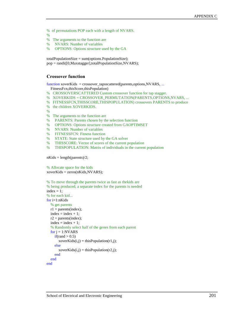
APPENDIX C
School of Electrical and Electronic Engineering 201
% of permutations POP each with a length of NVARS. % % The arguments to the function are % NVARS: Number of variables % OPTIONS: Options structure used by the GA totalPopulationSize = sum(options.PopulationSize); pop = randi([0,Maxstagger],totalPopulationSize,NVARS);
Crossover function
function xoverKids = crossover_tapsscattered(parents,options,NVARS, ... FitnessFcn,thisScore,thisPopulation) % CROSSOVERSCATTERED Custom crossover function for tap stagger. % XOVERKIDS = CROSSOVER_PERMUTATION(PARENTS,OPTIONS,NVARS, ... % FITNESSFCN,THISSCORE,THISPOPULATION) crossovers PARENTS to produce % the children XOVERKIDS. % % The arguments to the function are % PARENTS: Parents chosen by the selection function % OPTIONS: Options structure created from GAOPTIMSET % NVARS: Number of variables % FITNESSFCN: Fitness function % STATE: State structure used by the GA solver % THISSCORE: Vector of scores of the current population % THISPOPULATION: Matrix of individuals in the current population nKids = length(parents)/2; % Allocate space for the kids xoverKids = zeros(nKids,NVARS); % To move through the parents twice as fast as thekids are % being produced, a separate index for the parents is needed index = 1; % for each kid... for i=1:nKids % get parents r1 = parents(index); index = index + 1; r2 = parents(index); index = index + 1; % Randomly select half of the genes from each parent for j = 1:NVARS if(rand > 0.5) xoverKids(i,j) = thisPopulation(r1,j); else xoverKids(i,j) = thisPopulation(r2,j); end end end
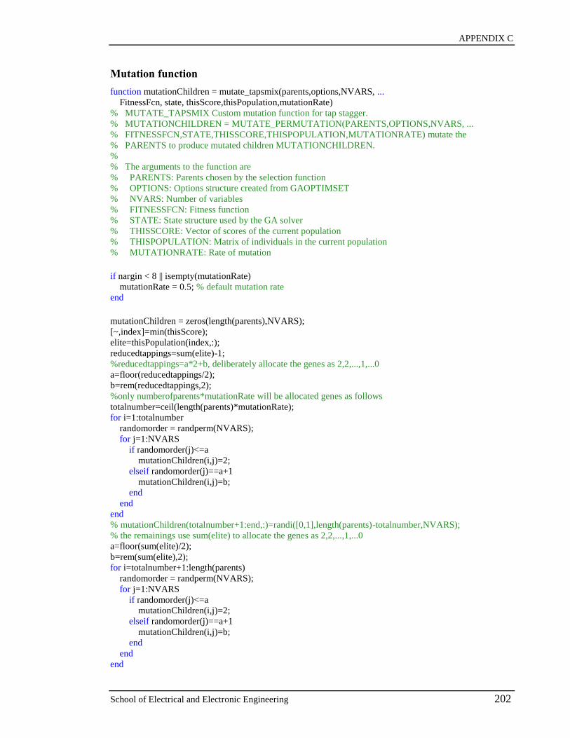
APPENDIX C
School of Electrical and Electronic Engineering 202
Mutation function
function mutationChildren = mutate_tapsmix(parents,options,NVARS, ... FitnessFcn, state, thisScore,thisPopulation,mutationRate) % MUTATE_TAPSMIX Custom mutation function for tap stagger. % MUTATIONCHILDREN = MUTATE_PERMUTATION(PARENTS,OPTIONS,NVARS, ... % FITNESSFCN,STATE,THISSCORE,THISPOPULATION,MUTATIONRATE) mutate the % PARENTS to produce mutated children MUTATIONCHILDREN. % % The arguments to the function are % PARENTS: Parents chosen by the selection function % OPTIONS: Options structure created from GAOPTIMSET % NVARS: Number of variables % FITNESSFCN: Fitness function % STATE: State structure used by the GA solver % THISSCORE: Vector of scores of the current population % THISPOPULATION: Matrix of individuals in the current population % MUTATIONRATE: Rate of mutation if nargin < 8 || isempty(mutationRate) mutationRate = 0.5; % default mutation rate end mutationChildren = zeros(length(parents),NVARS); [~,index]=min(thisScore); elite=thisPopulation(index,:); reducedtappings=sum(elite)-1; %reducedtappings=a*2+b, deliberately allocate the genes as 2,2,...,1,...0 a=floor(reducedtappings/2); b=rem(reducedtappings,2); %only numberofparents*mutationRate will be allocated genes as follows totalnumber=ceil(length(parents)*mutationRate); for i=1:totalnumber randomorder = randperm(NVARS); for j=1:NVARS if randomorder(j)<=a mutationChildren(i,j)=2; elseif randomorder(j)==a+1 mutationChildren(i,j)=b; end end end % mutationChildren(totalnumber+1:end,:)=randi([0,1],length(parents)-totalnumber,NVARS); % the remainings use sum(elite) to allocate the genes as 2,2,...,1,...0 a=floor(sum(elite)/2); b=rem(sum(elite),2); for i=totalnumber+1:length(parents) randomorder = randperm(NVARS); for j=1:NVARS if randomorder(j)<=a mutationChildren(i,j)=2; elseif randomorder(j)==a+1 mutationChildren(i,j)=b; end end end

APPENDIX D
School of Electrical and Electronic Engineering 203
APPENDIX D
MATLAB Codes for the Rule-based Control Scheme
Main function
clear;
tic;
fstarting=fopen('startingposition.txt');
ftap=fopen('tapchanger.txt');
record=textscan(fstarting,'%*s%*c%*c%*c%*c%f%*[^\n]');
startingpos=cell2mat(record);
%record the MaxTap, MinTap and NumTaps
tap=ones(length(startingpos),3);
while ~feof(ftap)
record=textscan(ftap,'%*s%*c%d',1,'delimiter','.'); %record the NO. of transformer
i=record{1};
record=textscan(ftap,'%*s%*c%*c%*c%*c%*c%*c%*c%f%*c%*c%*c%*c%*c%*c%*c%f%*c%*c%*c
%*c%*c%*c%*c%*c%f%*[^\n]',1);
tap(i,:)=cell2mat(record);
record=textscan(ftap,'%s%*[^\n]',1); %skip the next line
end
%change the NumTaps to TapStep(%)
tap(:,3)=round((tap(:,1)-tap(:,2))./tap(:,3)*10000)/100;
%Specify the tested primary transformers (A,B,C,D,E,F,G,H,I,J,K)
testedtrans=[31 30 20 21 23 22 24 25 28 29 26 27 7 6 13 14 11 10 9 8 5 4];
numberOfVariables=length(testedtrans)/2;
%Read the absorption capacity matrix (at 400kV side)
capmatrix=xlsread('capacitymatrix.xlsx','Additional Qloss');
capmatrixP=xlsread('capacitymatrix.xlsx','Additional Ploss');
%Specify the required MVAr absorption and the error allowance (%)
Qref=2.0;
allowanceQ=1.0;
Maxstagger=2;
%the maximum VAr could be provided at each staggering (among all the tested transformers)
Maxvar=zeros(2,Maxstagger);
Qactual=0.0;
Addvar=0;
Minerror=100;
Optimtap=zeros(1,numberOfVariables);
%build available capacity matrix from the already absorption Qactual
capavailable=capmatrix;
numofiterations=0;
while (Minerror>allowanceQ)
%eliminate the used transformer pair
if(Addvar>0)
capavailable(Maxvar(2,staggerno),:)=0;
end

APPENDIX D
School of Electrical and Electronic Engineering 204
%try to add VAr to Qactual and slowly accumulate to (1+allowancQ/100)*Qref
indices=find(capavailable>((1+allowanceQ/100)*Qref-Qactual));
capavailable(indices)=0;
%find the max VAr could be provided from 1,2,...staggering
for j=1:Maxstagger
[Maxvar(1,j) Maxvar(2,j)]=max(capavailable(:,j)); %also recording the row number, which indicates
the transformer NO.
end
%add the maximum VAr/pair in order to reduce number of tappings (based on
VAr(2tappings)>4*VAr(1tapping))
[Addvar,staggerno]=max(Maxvar(1,:));
if(Addvar==0)
break;
end
Optimtap(1,Maxvar(2,staggerno))=staggerno;
Qactual=Qactual+Addvar;
Minerror=abs(Qactual-Qref)/Qref*100;
numofiterations=numofiterations+1;
end
if (Minerror<=allowanceQ)
disp('A solution is found.');
else
disp('A solution is NOT found.');
end
Resultcount=tabulate(Minerror);
totaltappings=sum(Optimtap,2)*2; %pairs of two transformers
% Ploss=Minobj-totaltappings/2;
fclose(fstarting);
fclose(ftap);
CalculatingTime=toc;
Function for calculating the VAr absorption capability matrix
clear;
[DSSStartOK, DSSObj, DSSText] = DSSStartup;
if DSSStartOK
%Initialization
fstarting=fopen('startingposition.txt');
ftap=fopen('tapchanger.txt');
record=textscan(fstarting,'%*s%*c%*c%*c%*c%f%*[^\n]');
startingpos=cell2mat(record);
%record the MaxTap, MinTap and NumTaps
tap=ones(length(startingpos),3);
i=1;
while ~feof(ftap)
record=textscan(ftap,'%*s%*c%d',1,'delimiter','.'); %record the NO. of transformer
i=record{1};
record=textscan(ftap,'%*s%*c%*c%*c%*c%*c%*c%*c%f%*c%*c%*c%*c%*c%*c%*c%f%*c%*c%*c
%*c%*c%*c%*c%*c%f%*[^\n]',1);
tap(i,:)=cell2mat(record);
record=textscan(ftap,'%s%*[^\n]',1); %skip the next line
end
%change the NumTaps to TapStep(%)

APPENDIX D
School of Electrical and Electronic Engineering 205
tap(:,3)=round((tap(:,1)-tap(:,2))./tap(:,3)*10000)/100;
%set up the OpenDSS interface variables
currentpath=cd;
DSSText.command=['Compile (' currentpath '\Master.dss)'];
DSSCircuit=DSSObj.ActiveCircuit;
DSSSolution=DSSCircuit.Solution;
DSSText.Command='Set Normvmaxpu=1.06';
DSSText.Command='Set Normvminpu=0.94';
DSSText.Command='Set Maxiter=100';
DSSText.Command='Set Maxcontroliter=30';
DSSText.Command='Set tolerance=0.000001';
DSSText.Command='New Energymeter.m1 Transformer.T33 1';
DSSText.Command='New Monitor.PQ_m1 Transformer.T33 2 Mode=1';
%Specify the tested primary transformers (A,B,C,D,E,F,G,H,I,J,K)
testedtrans=[31 30 20 21 23 22 24 25 28 29 26 27 7 6 13 14 11 10 9 8 5 4];
numberOfVariables=length(testedtrans)/2;
%Calculate the inital reactive power flow in the network
for i=1:numberOfVariables
DSSCircuit.Transformers.Name=['T' int2str(testedtrans(2*i-1))]; %e.g. the first one is from A_33_t11
to A_6_a
DSSCircuit.Transformers.Wdg=1;
DSSCircuit.Transformers.Tap=startingpos(testedtrans(2*i-1));
DSSCircuit.Transformers.Name=['T' int2str(testedtrans(2*i))]; %e.g. the first one is from A_33_t12 to
A_6_b
DSSCircuit.Transformers.Wdg=1;
DSSCircuit.Transformers.Tap=startingpos(testedtrans(2*i));
end
DSSSolution.Solve;
if DSSSolution.Converged
MyElement=DSSCircuit.CktElements('Transformer.T33');
Qpre=MyElement.Powers(10)*-3/1.0e3; %the output power from T33 (400/275kV) in MVAr
Ppre=DSSCircuit.Losses(1)/1.0e6-MyElement.Losses(1)/1.0e6; %the distribution system loss in MW
else
disp('Not converged!1');
end
DSSText.Command='Init';
Maxstagger=2; %the maximum tap steps increased/decreased
T33P=zeros(numberOfVariables,Maxstagger);
T33Q=zeros(numberOfVariables,Maxstagger);
for i=1:numberOfVariables
for j=1:Maxstagger
DSSCircuit.Transformers.Name=['T' int2str(testedtrans(2*i-1))]; %e.g. the first one is from
A_33_t11 to A_6_a
DSSCircuit.Transformers.Wdg=1;
DSSCircuit.Transformers.Tap=startingpos(testedtrans(2*i-1))-j*tap(testedtrans(2*i-1),3)/100;
DSSCircuit.Transformers.Name=['T' int2str(testedtrans(2*i))]; %e.g. the first one is from A_33_t12
to A_6_b
DSSCircuit.Transformers.Wdg=1;
DSSCircuit.Transformers.Tap=startingpos(testedtrans(2*i))+j*tap(testedtrans(2*i),3)/100;
DSSSolution.Solve;
if DSSSolution.Converged
MyElement=DSSCircuit.CktElements('Transformer.T33');
T33P(i,j)=DSSCircuit.Losses(1)/1.0e6-MyElement.Losses(1)/1.0e6;
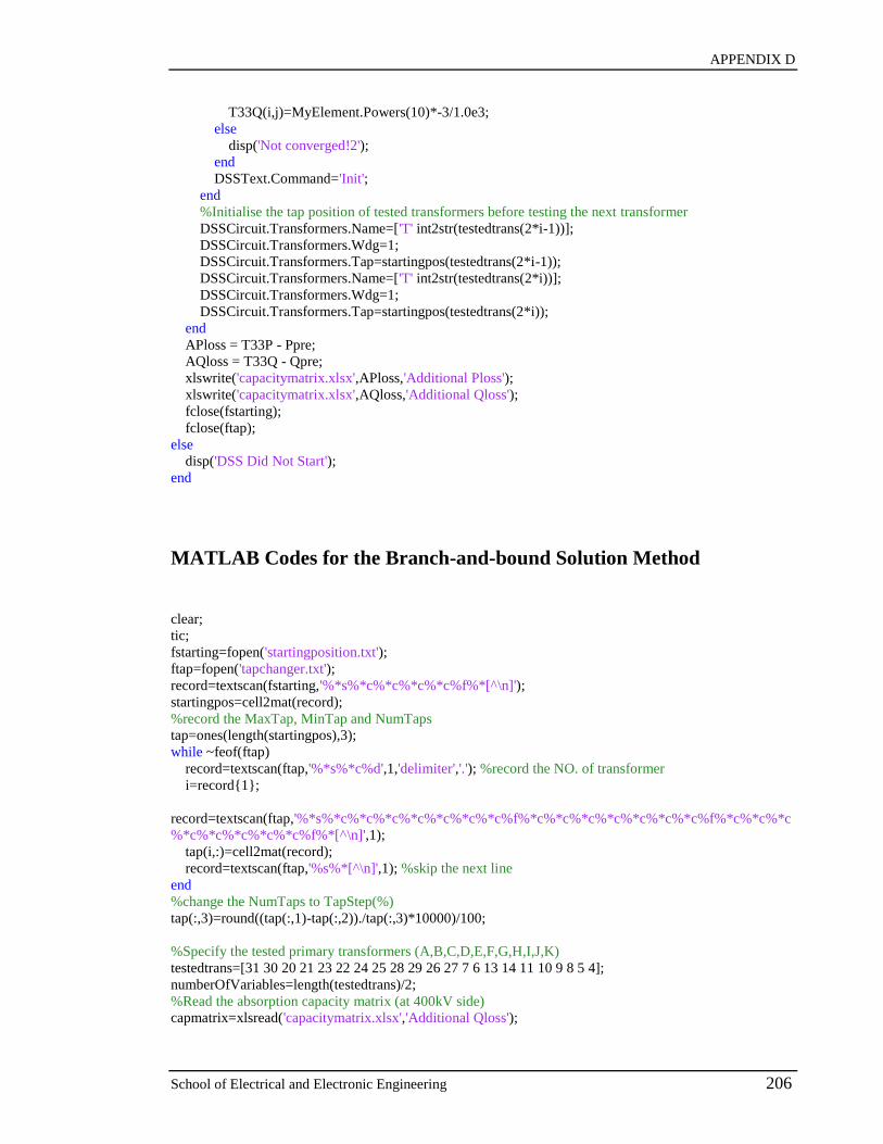
APPENDIX D
School of Electrical and Electronic Engineering 206
T33Q(i,j)=MyElement.Powers(10)*-3/1.0e3;
else
disp('Not converged!2');
end
DSSText.Command='Init';
end
%Initialise the tap position of tested transformers before testing the next transformer
DSSCircuit.Transformers.Name=['T' int2str(testedtrans(2*i-1))];
DSSCircuit.Transformers.Wdg=1;
DSSCircuit.Transformers.Tap=startingpos(testedtrans(2*i-1));
DSSCircuit.Transformers.Name=['T' int2str(testedtrans(2*i))];
DSSCircuit.Transformers.Wdg=1;
DSSCircuit.Transformers.Tap=startingpos(testedtrans(2*i));
end
APloss = T33P - Ppre;
AQloss = T33Q - Qpre;
xlswrite('capacitymatrix.xlsx',APloss,'Additional Ploss');
xlswrite('capacitymatrix.xlsx',AQloss,'Additional Qloss');
fclose(fstarting);
fclose(ftap);
else
disp('DSS Did Not Start');
end
MATLAB Codes for the Branch-and-bound Solution Method
clear;
tic;
fstarting=fopen('startingposition.txt');
ftap=fopen('tapchanger.txt');
record=textscan(fstarting,'%*s%*c%*c%*c%*c%f%*[^\n]');
startingpos=cell2mat(record);
%record the MaxTap, MinTap and NumTaps
tap=ones(length(startingpos),3);
while ~feof(ftap)
record=textscan(ftap,'%*s%*c%d',1,'delimiter','.'); %record the NO. of transformer
i=record{1};
record=textscan(ftap,'%*s%*c%*c%*c%*c%*c%*c%*c%f%*c%*c%*c%*c%*c%*c%*c%f%*c%*c%*c
%*c%*c%*c%*c%*c%f%*[^\n]',1);
tap(i,:)=cell2mat(record);
record=textscan(ftap,'%s%*[^\n]',1); %skip the next line
end
%change the NumTaps to TapStep(%)
tap(:,3)=round((tap(:,1)-tap(:,2))./tap(:,3)*10000)/100;
%Specify the tested primary transformers (A,B,C,D,E,F,G,H,I,J,K)
testedtrans=[31 30 20 21 23 22 24 25 28 29 26 27 7 6 13 14 11 10 9 8 5 4];
numberOfVariables=length(testedtrans)/2;
%Read the absorption capacity matrix (at 400kV side)
capmatrix=xlsread('capacitymatrix.xlsx','Additional Qloss');
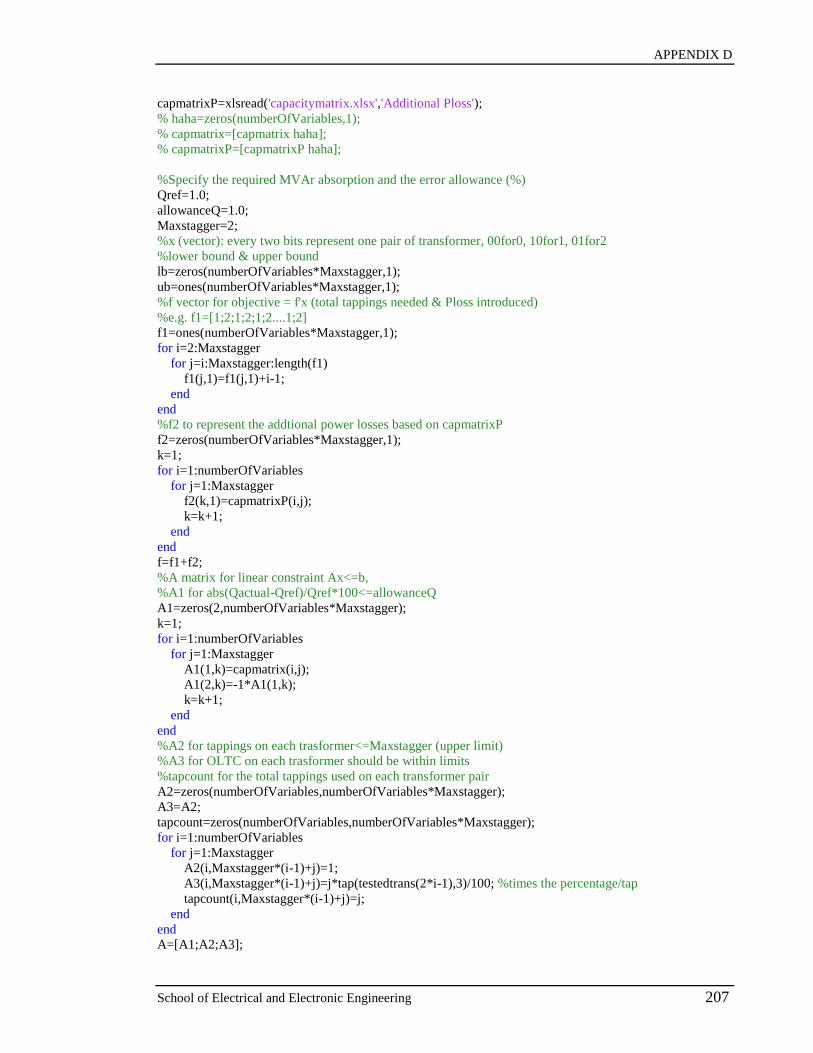
APPENDIX D
School of Electrical and Electronic Engineering 207
capmatrixP=xlsread('capacitymatrix.xlsx','Additional Ploss');
% haha=zeros(numberOfVariables,1);
% capmatrix=[capmatrix haha];
% capmatrixP=[capmatrixP haha];
%Specify the required MVAr absorption and the error allowance (%)
Qref=1.0;
allowanceQ=1.0;
Maxstagger=2;
%x (vector): every two bits represent one pair of transformer, 00for0, 10for1, 01for2
%lower bound & upper bound
lb=zeros(numberOfVariables*Maxstagger,1);
ub=ones(numberOfVariables*Maxstagger,1);
%f vector for objective = f'x (total tappings needed & Ploss introduced)
%e.g. f1=[1;2;1;2;1;2....1;2]
f1=ones(numberOfVariables*Maxstagger,1);
for i=2:Maxstagger
for j=i:Maxstagger:length(f1)
f1(j,1)=f1(j,1)+i-1;
end
end
%f2 to represent the addtional power losses based on capmatrixP
f2=zeros(numberOfVariables*Maxstagger,1);
k=1;
for i=1:numberOfVariables
for j=1:Maxstagger
f2(k,1)=capmatrixP(i,j);
k=k+1;
end
end
f=f1+f2;
%A matrix for linear constraint Ax<=b,
%A1 for abs(Qactual-Qref)/Qref*100<=allowanceQ
A1=zeros(2,numberOfVariables*Maxstagger);
k=1;
for i=1:numberOfVariables
for j=1:Maxstagger
A1(1,k)=capmatrix(i,j);
A1(2,k)=-1*A1(1,k);
k=k+1;
end
end
%A2 for tappings on each trasformer<=Maxstagger (upper limit)
%A3 for OLTC on each trasformer should be within limits
%tapcount for the total tappings used on each transformer pair
A2=zeros(numberOfVariables,numberOfVariables*Maxstagger);
A3=A2;
tapcount=zeros(numberOfVariables,numberOfVariables*Maxstagger);
for i=1:numberOfVariables
for j=1:Maxstagger
A2(i,Maxstagger*(i-1)+j)=1;
A3(i,Maxstagger*(i-1)+j)=j*tap(testedtrans(2*i-1),3)/100; %times the percentage/tap
tapcount(i,Maxstagger*(i-1)+j)=j;
end
end
A=[A1;A2;A3];

APPENDIX D
School of Electrical and Electronic Engineering 208
%b matrix for linear constriant Ax<=b
b1=[Qref*(1+allowanceQ/100);-1*Qref*(1-allowanceQ/100)];
b2=ones(numberOfVariables,1); %1,2,3,...,Maxstagger can only occur once
b3=zeros(numberOfVariables,1);
for i=1:numberOfVariables
gaptoupper=tap(testedtrans(2*i-1),1)-startingpos(testedtrans(2*i-1)); %max-startingpos
gaptolower=-1*tap(testedtrans(2*i),2)+startingpos(testedtrans(2*i)); %-min+startingpos
b3(i,1)=min(gaptoupper,gaptolower);
end
b=[b1;b2;b3];
%starting points for the optimisation
%x0=ub;
x0=lb;
% bintprog options
options = optimset('bintprog');
options = optimset(options,'Diagnostics','off','Display','iter','TolFun',1.0e-6,
'MaxNodes',100000*numberOfVariables*Maxstagger);
Runtimes=1;
Minobj=zeros(Runtimes,1); %value of objective function
Minerror=zeros(Runtimes,1); %percentage error between Qactual and Qref
Optimtap1=zeros(Runtimes,numberOfVariables*Maxstagger);
Optimtap=zeros(Runtimes,numberOfVariables);
for i=1:Runtimes
disp(['Iteration No.' num2str(i) ' starts']);
[x,fval,exitflag,output] = bintprog(f,A,b,[],[],[],options);
if exitflag>0
Minobj(i,1)=fval;
Optimtap1(i,:)=x';
tapaction=A*x;
Optimtap(i,:)=(tapcount*x)';
Minerror(i,1)=abs(tapaction(1,1)-Qref)/Qref*100;
end
%disp(['Iteration No.' num2str(i) ', ' output.message]);
end
Resultcount=tabulate(Minerror);
totaltappings=sum(Optimtap,2)*2; %pairs of two transformers
Ploss=Minobj-totaltappings/2;
fclose(fstarting);
fclose(ftap);
CalculatingTime=toc;

APPENDIX E
School of Electrical and Electronic Engineering 209
APPENDIX E
222-Bus Distribution Network Model
The 222-bus distribution network model is illustrated in Figure B. This network is part of
the large distribution system shown in Figure A. It includes a 132kV GSP and the entire
downstream 33kV networks connected to the GSP. The 222-bus network model has first
been extracted from the original IPSA network model shown in Figure A and then it has
been converted to OpenDSS circuit description files.
Due to confidentiality agreements, Table B can only list some basic data of the 222-bus
distribution system model.
Table B: Quantities of different network components of the 222-bus model
Quantity
Buses 400kV: 1
275kV: 5
132kV: 38
33kV: 120
11kV: 18
6.6kV: 40
Lines 192
Transformers 76
Static Loads
(constant load model)
66 (with a total of 427 MW and 127MVAr)
GSPs 1
33kV Load Areas 6
Primary Substations 28
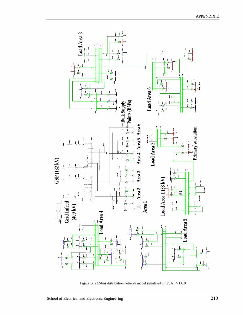
APPENDIX E
School of Electrical and Electronic Engineering 210
Gri
d In
feed
(400
kV
)
GSP
(132
kV
)
Bul
k Su
pply
Poi
nts
(BSP
s)
To
Are
a 1
Are
a 2
Are
a 3
Are
a 4
Are
a 5
Are
a 6
Loa
d A
rea
1 (3
3 kV
)
Loa
d A
rea
2
Loa
d A
rea
3
Loa
d A
rea
4
Loa
d A
rea
5
Loa
d A
rea
6
# 1
Pri
mar
y su
bsta
tion
Figure B: 222-bus distribution network model simulated in IPSA+ V1.6.8